


Abstract
The Human Learning Optimization (HLO) algorithm is a binary metaheuristic algorithm that simulates human random learning, individual learning, and social learning processes. Owing to its simple structure and low computational cost, HLO has been widely applied to continuous optimization and machine-learning hyperparameter tuning. However, when applied to continuous optimization, the original HLO suffers from three major limitations: the Hamming cliff phenomenon associated with standard binary encoding, the limited source of knowledge for social learning, and an almost fixed learning probability. To address these issues, this study proposes a Gray-code and successful-memory human learning optimization algorithm based on a pretrained language model, termed LGSM-HLO. Specifically, the Pre-trained Language Model-Inspired Strategy (PLMS) treats elite encodings as a knowledge corpus and extracts shared encoding patterns through weighted pretraining, masked reconstruction, and online fine-tuning. The Gray-code Coarse-to-Fine Semantic Learning strategy (GCFSL) employs Gray coding to improve encoding-neighborhood consistency and dynamically adjusts the learning granularity throughout the evolutionary process. The Successful-History Differential Teacher Strategy (SHDTS) integrates historical successful parameters, high-quality individuals, and population differential information to construct personalized social teachers, while providing a Cauchy-based escape mechanism for stagnated individuals. Experiments on the CEC2017 (30-dimensional) and CEC2022 (10- and 20-dimensional) benchmark suites show that LGSM-HLO achieves superior mean performance and standard deviation on most functions compared with nine competitive algorithms. The Wilcoxon rank-sum test and Friedman rank test further confirm its overall superiority. Moreover, none of the three proposed strategies introduces additional objective-function evaluations, and the proposed algorithm retains the same dominant asymptotic computational complexity as the original HLO. Furthermore, an LGSM-HLO-RF model is developed by employing LGSM-HLO for joint hyperparameter optimization of a random forest. In the three-class prediction of higher-education student achievement, LGSM-HLO-RF outperforms the comparison algorithms in terms of Accuracy, Macro-F1, and Macro-Recall, demonstrating the strong transferability of LGSM-HLO from benchmark optimization to practical educational data-mining tasks.
1. Introduction
With the rapid development of intelligent manufacturing, energy systems, communication networks, data science, and artificial intelligence, a growing number of real-world problems have exhibited complex characteristics, including high dimensionality, nonlinearity, multimodality, nonconvexity, nondifferent ability, strong coupling, and black-box evaluation [1,2,3]. For such problems, the objective functions are often difficult to formulate explicitly in analytical form and may even be intractable using conventional mathematical optimization methods. Meanwhile, as the dimensionality of decision variables increases, the search space expands exponentially, making exhaustive search and conventional deterministic optimization methods difficult to use in obtaining satisfactory solutions under limited computational resources. Therefore, how to effectively balance global exploration and local exploitation in complex search spaces, while avoiding premature convergence and maintaining high convergence speed and solution stability, has become an important research issue in the field of intelligent optimization [4,5]. Traditional gradient-based and mathematical programming methods generally rely on prior assumptions such as continuity, differentiability, or convexity of the objective function, whereas many real-world optimization problems do not satisfy these requirements [6,7,8]. In contrast, metaheuristic optimization algorithms generally do not require gradient information and can directly guide the search through fitness evaluations. Consequently, they have been widely applied to complex engineering optimization, parameter tuning, machine learning, and data-driven decision-making.
In recent years, swarm intelligence and bio-inspired metaheuristic algorithms have developed rapidly, resulting in a diverse algorithmic framework that includes Particle Swarm Optimization (PSO) [9], Whale Optimization Algorithm (WOA) [10], Grey Wolf Optimizer (GWO) [11], Differential Evolution (DE) [12], Ant Colony Optimization (ACO) [13], and various other nature-inspired optimization methods. These algorithms typically establish search strategies by simulating collective cooperation, predatory behavior, migration, competition, or survival mechanisms in nature, and iteratively optimize candidate solutions through position updating, stochastic perturbation, and elite preservation mechanisms. For example, Modified Particle Swarm Optimization (MPSO) improves search performance by modifying the particle velocity update mechanism [14]. Dynamic Gold Rush Optimizer (DGRO) enhances high-dimensional search capability through a multi population mechanism [15]. Artificial Rabbits Optimization (ARO) [16] achieves a balance between global exploration and local exploitation by simulating the foraging and survival behaviors of rabbits. More recently, the Gekko Japonicus Algorithm (GJA) [17], Bounty hunter optimizer (BHO) [18], Secretary bird optimization algorithm (SBOA) [19], sled dog-inspired optimizer (SDO) [20], Bounty Hunter Optimizer (BHO) [18], and Dung Beetle Optimizer (DBO) [21] have further improved the search performance of metaheuristic algorithms from different perspectives, including neighborhood variation, reinforcement learning, heat-transfer-inspired search, oscillatory exploration, and relative-individual selection.
Despite their simple structures, weak requirements on objective functions, and broad applicability, metaheuristic optimization algorithms inherently face a trade-off between exploration and exploitation. On the one hand, excessive stochastic exploration can maintain population diversity and enlarge the search range, but may reduce the convergence rate and lead to inefficient searches during the later optimization stage [8,22]. On the other hand, excessive reliance on the current best solution can rapidly concentrate search resources, but may cause the population to prematurely converge toward a local optimum, thereby reducing its ability to escape from local optima [7,23]. In addition, the control parameters of many algorithms are predetermined or simply varied according to the iteration number, and therefore cannot sufficiently reflect individual quality, population status, or historical search experience [24,25]. Consequently, effectively exploiting high-quality historical knowledge generated during the search process and dynamically adapting search behaviors according to different optimization stages and individual states have become important directions for further improving metaheuristic optimization algorithms.
Inspired by human learning mechanisms, Zhang et al. proposed the Human Learning Optimization (HLO) algorithm [26]. HLO interprets the optimization process as a knowledge acquisition process and simulates human learning from unknown information, individual historical experience, and superior individuals through three learning mechanisms: random learning, individual learning, and social learning. Meanwhile, HLO establishes an Individual Knowledge Database (IKD) and a Social Knowledge Database (SKD) to preserve the historically best individual knowledge and historically best population knowledge, respectively, thereby combining current search information with successful historical experience. This knowledge-learning perspective provides a distinct alternative to conventional position-update models for metaheuristic optimization and enables the algorithm to explicitly preserve and exploit historical experience during the search process. However, the employs a binary-coded knowledge representation and simulates three fundamental learning behaviors: random learning, individual learning, and social learning. Its knowledge-learning mechanism provides a flexible framework for binary-encoded optimization problems. When this representation is extended to continuous optimization through binary-to-real decoding, however, several potential limitations deserve further consideration. First, conventional binary representations may exhibit the Hamming-cliff phenomenon, in which adjacent numerical values correspond to substantially different binary strings. Second, the social-learning mechanism primarily exploits the best knowledge stored in the SKD, which may limit the utilization of shared patterns distributed among multiple high-quality individuals. Third, the learning probabilities are not explicitly adapted to the significance of individual coding positions or to historically successful search parameters. These observations motivate the investigation of alternative encoding representations, population-level knowledge modeling, and adaptive social-learning mechanisms. It should be emphasized that these limitations are identified from the algorithmic structure and the requirements of continuous optimization rather than interpreted as universal performance deficiencies of the original HLO.
To address the issues of knowledge utilization and parameter adaptation in metaheuristic algorithms, an increasing number of studies have recently attempted to incorporate learning mechanisms, memory mechanisms, and multi-source information fusion. One line of research introduces reinforcement learning, adaptive feedback, or dynamic probability adjustment to enable algorithms to select different search behaviors according to the current search state [27]. Another line of research enhances information exchange among populations through elite learning, multi population cooperation, and differential information [28,29]. Other studies record historically successful parameters to preserve effective search behaviors, allowing control parameters to gradually adapt to the characteristics of the optimization problem. These studies indicate that relying solely on the current position or the current best individual is insufficient for addressing complex optimization tasks. Instead, shared patterns among multiple high-quality solutions, historical search experience, and relative differences among individuals can provide additional information for constructing more effective search directions [30]. However, existing enhancement mechanisms often operate independently at a single level, such as search strategy, parameter adaptation, or population cooperation. A unified framework is still lacking for addressing the interconnected questions of how knowledge should be represented, how knowledge at different granularities should be selected at different optimization stages, and how personalized social knowledge should be generated according to individual states.
Recent studies have further demonstrated the potential of intelligent optimization and multi-strategy learning mechanisms in complex decision-making problems. For instance, the integration of particle swarm optimization with large language models for automatic prompt design in medical information extraction illustrates how population-based search can be combined with language-oriented representations to improve task-specific performance [31]. Research on truthful combinatorial double auctions for mobile edge computing in the Industrial Internet of Things also highlights the importance of efficient optimization and resource allocation in complex computational environments [32].
Meanwhile, multi-strategy improvements to the Northern Goshawk Optimization algorithm and the Enterprise Development Optimizer demonstrate the potential benefits of incorporating complementary search mechanisms to improve optimization performance across benchmark and engineering problems [33,34]. In addition, research on the enhanced evolution of parallel algorithm portfolios for vehicle routing problems through transfer optimization illustrates the value of exploiting knowledge accumulated across different search processes [35].
Although these studies address different optimization tasks and employ different algorithmic frameworks, they collectively emphasize the importance of knowledge utilization, adaptive search, and complementary optimization mechanisms. Motivated by these developments, the present study focuses on improving the original HLO framework through elite-encoding probability modeling, Gray-coded coarse-to-fine learning, and personalized social-teacher construction.
Meanwhile, the performance of machine-learning models is also strongly affected by parameter configurations. In recent years, machine learning has increasingly been applied to educational data analysis, where information such as student demographics, family background, learning behavior, attendance, previous academic achievement, and course-related characteristics can be used to predict students’ final academic performance, thereby providing auxiliary decision support for instructional intervention, student management, and personalized education [36,37]. Compared with manually configuring model parameters based solely on empirical experience, intelligent optimization algorithms can formulate machine-learning hyperparameter configuration as a black-box optimization problem and search iteratively for parameter combinations that are better suited to a specific dataset. Among various machine-learning methods, Random Forest (RF) provides strong nonlinear modeling capability and good robustness. By integrating multiple decision trees, RF can also reduce the variance associated with individual trees, making it suitable for student achievement classification involving small-scale datasets and heterogeneous features [38,39].
Although RF generally exhibits strong classification capability, its performance is jointly affected by multiple hyperparameters. In this study, the parameters considered for optimization include the number of decision trees, the minimum number of observations required at leaf nodes, the number of predictor variables sampled at each node split, and the maximum number of splits. These parameters respectively affect the ensemble size, structural complexity of the trees, feature-level randomness, and representational capacity of individual trees, while exhibiting considerable interactions with one another. Therefore, sequentially tuning individual parameters cannot guarantee an optimal overall configuration.
Based on the above analysis, the primary objective of this study is not to simply stack multiple search operators, but to establish a unified improvement framework around three key bottlenecks of the original HLO from the perspectives of knowledge representation, encoding-level learning, and social teacher construction, thereby developing the LGSM-HLO algorithm.
To address the limitation of a single knowledge source, the Pretrained Language Model Strategy (PLMS) is proposed. It treats the complete Gray-coded representations of multiple elite individuals as a high-quality knowledge corpus and extracts shared encoding patterns through weighted probabilistic modeling, confidence estimation, elite prototype selection, masked reconstruction, and online fine-tuning. Here, the term “language model” refers to a lightweight elite-encoding probabilistic model established during the optimization process rather than an external natural-language model. To address the discontinuity of encoding neighborhoods, the Gray-code Coarse-to-Fine Semantic Learning (GCFSL) strategy is developed. By exploiting the property of Gray coding that adjacent integers typically differ by only one bit, GCFSL improves neighborhood consistency between the encoding space and the continuous search space. According to the different effects of encoding bits on numerical values, higher-order bits are regarded as coarse-grained information for controlling regional search, whereas lower-order bits represent fine-grained information for controlling search precision. The learning emphasis is gradually shifted from higher-order bits to lower-order bits as the optimization proceeds, thereby achieving a progressive transition from regional exploration to fine-grained exploitation. To address the lack of individual differentiation in social learning and the insufficient utilization of historical parameters, the Successful-History Differential Teacher Strategy (SHDTS) is proposed. SHDTS integrates the current individual, high-quality individuals, and population differential information to construct differential teachers in the continuous space. Historical successful parameter memories are used to dynamically generate scaling factors and crossover probabilities. When an individual remains unimproved for an extended period, a heavy-tailed Cauchy perturbation is employed to generate an escape teacher, helping the individual move beyond the local attraction basin. The resulting continuous teacher is subsequently converted back into Gray coding and integrated with the PLMS elite knowledge templates and the global-best knowledge stored in the SKD to construct a personalized social teacher.
The three strategies do not independently introduce additional search operators but operate at different information levels: PLMS models shared knowledge within the population, GCFSL dynamically regulates the search granularity, and SHDTS integrates search direction, individual state, and historical successful parameters to generate adaptive teachers. These strategies are jointly embedded into the original random learning, individual learning, and social learning framework of HLO while retaining the IKD and SKD knowledge-update mechanisms. Without altering the fundamental learning paradigm of HLO, the proposed framework provides richer knowledge sources, more appropriate search scales, and more flexible social learning directions.
The methodological contribution of this study is not the independent invention of Gray coding, differential mutation, or success-history parameter adaptation. Rather, it lies in establishing a unified HLO-based learning framework in which elite-encoding probability modeling provides population-level knowledge, Gray-coded coarse-to-fine learning regulates the utilization of encoded information, and success-history differential teacher construction supplies individualized social-learning targets. These mechanisms operate at different levels of the original HLO learning process and are integrated without replacing its fundamental random-learning, individual-learning, and social-learning structure.
The remainder of this paper is organized as follows: Section 2 first introduces the original HLO and then presents the three proposed improvement strategies, namely PLMS, GCFSL, and SHDTS, together with the overall optimization procedure and computational complexity analysis. Section 3 systematically evaluates LGSM-HLO on the CEC2017 and CEC2022 benchmark functions and further assesses its performance through statistical tests and Friedman ranking. Section 4 presents the three-class student academic achievement prediction model based on LGSM-HLO-RF, including the dataset, RF classification model, hyperparameter optimization procedure, and experimental evaluation. Finally, Section 5 summarizes the main findings of this study and discusses the current limitations and potential directions for future research.
2. The Proposed Language-Guided Gray-Coded and Success-Memory Human Learning Optimization
2.1. The Original Human Learning Optimization Algorithm
Human Learning Optimization (HLO) is a binary-coded metaheuristic inspired by the knowledge-acquisition process of human beings [26]. It assumes that humans acquire knowledge through three fundamental behaviors: random learning, individual learning, and social learning. Random learning introduces unknown information through trial and error, individual learning retrieves successful experience accumulated by the learner, and social learning acquires high-quality knowledge from the most successful member of the population. To preserve these two types of historical experience, HLO establishes an Individual Knowledge Database (IKD) for each individual and a Social Knowledge Database (SKD) for the entire population.
For consistency with the subsequent LGSM-HLO, a bound-constrained minimization problem is considered. Let N denote the population size, D the problem dimension, t the current iteration, and TT the maximum number of iterations. The real-valued solution of the i-th individual at iteration t is represented by
The lower and upper bounds of the search space are denoted by
lb = [lb1,lb2,…,lbD],ub = [ub1,ub2,…,ubD].
Each decision variable is represented using K bits. In this study, K = 32, and the total coding length of an individual is therefore L = KD. The binary-coded sequence of the i-th individual is expressed as [26]
During initialization, every coding position is independently assigned zero or one with equal probability [26]:
Let denote the k-th bit associated with the j-th decision variable of the i-th individual. The corresponding nonnegative integer is calculated as
The integer value is then mapped to the actual search interval according to
After decoding the initial binary population, the objective value of each individual is evaluated. The initial code of every individual is stored in the IKD. The IKD is represented as [26]:
where denotes the historically best binary knowledge of the i-th individual. At initialization,
where denotes the historical best fitness value of the i-th individual.
The best knowledge discovered by the entire population is stored in the SKD. For a minimization problem, the index of the global-best individual and the corresponding social knowledge are determined by
At each iteration, HLO probabilistically selects random learning, individual learning, or social learning for every coding position. The random-learning and individual-learning thresholds are defined as [26]
The thresholds in Equation (10) follow the probabilistic learning framework of the original HLO [26]. Rather than representing independent probabilities, they define cumulative decision boundaries for selecting the three learning behaviors. Specifically, the random-learning probability corresponds to the first threshold, the individual-learning probability corresponds to the difference between the second and first thresholds, and the remaining probability is assigned to social learning.
This cumulative-threshold formulation ensures that the three learning probabilities are nonnegative and sum to one, provided that the thresholds satisfy the required ordering constraints. Random learning introduces new information, individual learning exploits historically successful personal knowledge, and social learning acquires knowledge from superior solutions. The thresholds therefore regulate the relative frequencies of exploration, personal experience utilization, and social knowledge acquisition.
Accordingly, the probabilities of performing random learning, individual learning, and social learning are pR, pI − pR, and 1 − pI, respectively. Let be an independently generated random number. The human learning operator is formulated as
The first branch randomly assigns zero or one to introduce new knowledge and maintain population diversity. The second branch retrieves the historically best personal knowledge stored in the IKD. The third branch imitates the global-best knowledge stored in the SKD. Therefore, the three branches correspond to random learning, individual learning, and social learning, respectively [26].
After all coding positions have been updated, the new binary candidate is decoded into a real-valued solution and evaluated:
where the decoding procedure follows Equations (5) and (6). The new knowledge replaces the corresponding historical knowledge in the IKD only when it produces a better fitness value [26]:
After all IKD entries have been updated, the best historical knowledge is selected using Equation (9) to update the SKD. The learning, decoding, fitness-evaluation, IKD-updating, and SKD-updating procedures are repeated until the maximum number of iterations is reached. The real-valued solution decoded from sT is then returned as the final solution.
2.2. Language-Guided Gray-Coded and Success-Memory Human Learning Optimization
Although the original Human Learning Optimization (HLO) algorithm simulates the human knowledge-acquisition process through random learning, individual learning, and social learning, and preserves historical experience using the Individual Knowledge Database (IKD) and Social Knowledge Database (SKD), several limitations remain when it is applied to complex continuous optimization problems. First, the original HLO employs standard binary coding to represent continuous variables. When a real-valued solution crosses certain adjacent intervals, multiple binary bits may change simultaneously, resulting in the well-known Hamming-cliff phenomenon and weakening the neighborhood consistency between the coding space and the real-valued search space. Second, social learning in the original HLO mainly depends on the single global-best individual stored in the SKD. The common coding patterns contained in multiple elite individuals are not sufficiently utilized, which may result in a limited knowledge source and premature population convergence. Finally, the original HLO adopts nearly fixed learning probabilities without considering bit significance, evolutionary progress, individual quality, stagnation state, or historically successful parameters. Consequently, the algorithm may exhibit insufficient exploration during the early stage or limited convergence accuracy during the later stage.
To address these limitations, this study proposes the Language-Guided Gray-Coded and Success-Memory Human Learning Optimization algorithm, termed LGSM-HLO. Without changing the fundamental framework of the original HLO, including the binary population, random learning, individual learning, social learning, IKD updating, and SKD updating, LGSM-HLO incorporates three complementary enhancement strategies. First, a Pre-trained Language Models Strategy (PLMS) treats complete elite codes as high-quality knowledge corpora and extracts reliable coding patterns through weighted pre-training and online fine-tuning. Second, a Gray-Coded Coarse-to-Fine Semantic Learning (GCFSL) strategy employs Gray coding to improve the neighborhood continuity of encoded solutions and gradually transfers the learning focus from high-order bits to low-order bits. Finally, a Success-History Differential Teacher Strategy (SHDTS) constructs personalized social teachers using historically successful parameters, high-quality individuals, and population-difference information while providing an adaptive escape mechanism for stagnant individuals.
The three proposed strategies operate on knowledge modeling, coding-level learning, and social-teacher construction, respectively. PLMS expands the source of population knowledge, GCFSL coordinates the search granularity at different evolutionary stages, and SHDTS strengthens the directionality and parameter adaptability of social learning. Their cooperation improves convergence speed, optimization accuracy, and the ability to escape from local optima while retaining the concise knowledge-learning structure of the original HLO.
2.2.1. Pre-Trained Language Model-Inspired Strategy
In the original HLO, social learning primarily relies on the global-best knowledge stored in the SKD. Although this mechanism provides a clear learning direction, it cannot sufficiently exploit the shared encoding patterns distributed among multiple high-quality individuals. Excessive dependence on a single knowledge source may also accelerate the loss of population diversity.
To address this limitation, a Probabilistic Language-Inspired Modeling Strategy (PLMS) is introduced. Inspired by the concepts of token representation, corpus-based knowledge extraction, and masked reconstruction, PLMS regards elite Gray-coded solutions as structured binary sequences and constructs a lightweight probabilistic representation of their shared characteristics.
It is important to clarify that PLMS does not employ an externally pretrained large language model, a neural sequence model, or an explicit autoregressive conditional probability distribution. Instead, the strategy estimates fitness-weighted marginal probabilities at individual coding positions, selects complete elite prototypes to preserve existing encoding structures, and reconstructs selected positions according to elite consensus. The learned probability estimates are subsequently updated through exponential smoothing as the elite population evolves.
Consequently, the term “language-inspired” describes the conceptual analogy between elite encoding sequences and token-based knowledge representations, rather than the implementation of a conventional natural-language processing model. The main purpose of PLMS is to extract and reuse population-level encoding regularities within a computationally lightweight framework.
The principal process of PLMS is illustrated in Figure 1. The individual knowledge solutions are first ranked according to fitness. The best solutions are then selected to construct an elite binary corpus. Rank-based weights are used to measure their relative importance. Finally, the learned positional and contextual probabilities are combined to generate new language-guided binary tokens.
Figure 1.
Schematic illustration of the Pre-trained Language Models Strategy.
First, the individuals stored in the IKD are sorted in ascending order according to their fitness values, and the first Ne individuals are selected to form the elite knowledge corpus:
where denotes the Gray-coded sequence of the k-th elite individual. For a minimization problem, the elite individuals satisfy
Here, represents the fitness value obtained by decoding and evaluating .
To assign greater knowledge contributions to higher-quality elite individuals, an exponential weight is defined according to the fitness ranking:
Accordingly, the elite knowledge probability that the l-th coding position takes the value of one is calculated as
where denotes the bit value at the l-th position of the k-th elite code. A large indicates that the elite individuals tend to take the value of one at this position, whereas a small indicates a preference for zero.
The knowledge confidence and consensus bit at the l-th coding position are subsequently defined as
The value of lies within [0, 1]. When is close to zero or one, the elite individuals exhibit strong agreement at the corresponding position, resulting in a large confidence value. Conversely, when is close to 0.5, no stable knowledge pattern has been formed, and the corresponding confidence is low.
When generating a language-guided knowledge template, one complete elite code is first selected from t according to the probabilities wk. This complete-code selection preserves the structural relationship among different variables and coding positions. High-confidence positions are then reconstructed using a masked learning mechanism. Let denote the masking state of the l-th coding position:
The language-guided knowledge template is generated as
where is the selected elite prototype. Rather than independently generating every bit, this mechanism retains the complete structure of an elite code and reconstructs only the positions with sufficiently reliable elite consensus. It therefore reduces the probability of producing ineffective codes through arbitrary bit combinations.
As the population evolves, the composition of the elite corpus changes continuously. PLMS therefore employs an online fine-tuning mechanism to update the elite knowledge probability:
where is recalculated from the current elite corpus using Equation (18), and ηt is a dynamic learning rate defined as
ηt = 0.12[1 − 0.5λ(t)].
The online probability update in Equation (21) is implemented as an exponential smoothing operation. Specifically, the probability estimate obtained from the current elite population is combined with the previously stored estimate through a learning-rate coefficient. This mechanism allows newly discovered elite knowledge to influence the probability model while retaining information accumulated during earlier iterations.
The updated probabilities are constrained to the interval [0, 1] to ensure their validity as Bernoulli probability parameters. The learning-rate coefficient is controlled according to the evolutionary progress, as defined in Equation (22). Consequently, the probability model adapts to changes in the elite population without requiring gradient-based parameter optimization.
During the early stage, a relatively large learning rate enables the language-guided model to absorb newly discovered high-quality coding patterns rapidly. During the later stage, the learning rate gradually decreases to prevent excessive fluctuations in the learned probability distribution.
Through elite-corpus pre-training, confidence estimation, complete-prototype selection, masked reconstruction, and online fine-tuning, PLMS establishes an additional population-level knowledge representation beyond the single solution stored in the SKD. Consequently, the algorithm can exploit common patterns among multiple elite individuals while reducing excessive dependence on the current global-best code.
2.2.2. Gray-Coded Coarse-to-Fine Semantic Learning Strategy
Standard binary coding suffers from the Hamming-cliff phenomenon, in which two numerically adjacent integers may have considerably different binary representations. For example, the standard binary representations of the adjacent decimal numbers 7 and 8 are 0111 and 1000, respectively, requiring all four bits to change. For the bit-level learning process of HLO, such discontinuity can reduce the stability of local exploitation.
To improve neighborhood consistency between the coding space and the real-valued search space, GCFSL employs Gray coding to represent each decision variable. Let denote the nonnegative integer corresponding to the j-th decision variable of the i-th individual.
The mechanism of GCSL is illustrated in Figure 2. During the early stage, high-order semantic groups are emphasized to produce large-scale exploration. During the middle stage, intermediate groups are activated to improve regional search. During the late stage, low-order groups are emphasized to obtain fine numerical refinement.
Figure 2.
Schematic illustration of the Gray-Coded Coarse-to-Fine Semantic Learning Strategy.
The mapping from the real-valued variable to the integer representation is given by
where K = 32, and lbj and ubj are the lower and upper bounds of the j-th decision variable, respectively. The Gray-coded integer corresponding to is calculated as
where ⊕ denotes the bitwise exclusive-OR operator. In contrast to standard binary coding, two adjacent Gray-coded integers generally differ at only one bit position, thereby reducing abrupt changes between neighboring real-valued solutions.
For the decoding process, let and denote the k-th Gray bit and standard binary bit of the j-th variable, respectively. The conversion is performed as
After reconstructing the standard binary integer , the corresponding real-valued variable is obtained as
Although Gray coding improves neighborhood continuity, different coding positions still have different effects on the represented real value. High-order bits determine the approximate region in which the solution is located, whereas low-order bits mainly control numerical precision. Accordingly, a coarse-to-fine learning mechanism is introduced to regulate the search emphasis throughout the evolutionary process.
The normalized evolutionary progress and the normalized fitness rank of the i-th individual are defined as
For a minimization problem, . A small indicates a high-quality individual, whereas a large corresponds to a relatively poor individual.
The center and width of the bit-level learning region are defined as
Here, k = 1 represents the highest-order bit and k = K represents the lowest-order bit. During the early search stage, μ(t) is located near the high-order coding region, while the relatively large σ(t) maintains a broad learning range. As the iterations proceed, μ(t) gradually moves toward the low-order region and σ(t) decreases, allowing the algorithm to shift from broad regional exploration to fine-grained numerical refinement.
The curriculum weight of the k-th coding position is expressed as
The normalization in Equation (29) maintains an average weight of one. Therefore, the curriculum mechanism primarily redistributes random-learning opportunities among different coding positions without uncontrollably increasing the total amount of random perturbation.
Let denote the number of consecutive unsuccessful learning attempts experienced by the i-th individual. The expected number of randomly learned bits is defined as
The random-learning probability at the l-th coding position is then calculated as
where κ(l) ∈ {1,2,…,K} denotes the local bit order of the l-th coding position within its corresponding decision variable. The function clip(x,a,b) restricts xx to the interval [a,b].
The social-learning probability is defined as
and the individual-learning probability is correspondingly given by
Let ri,l∼U(0,1), and let denote the l-th bit of the personalized social teacher of the i-th individual. The improved human learning operator is formulated as
Equation (34) retains the three learning branches of the original HLO. Random learning generates new binary knowledge, individual learning retrieves the historically best knowledge stored in the IKD, and social learning acquires information from the personalized teacher generated by PLMS and SHDTS.
During the early stage, GCFSL focuses on high-order bits and broad regional exploration. During the later stage, the learning focus gradually moves toward low-order bits to improve numerical accuracy. Poor or stagnant individuals are assigned relatively large random-learning probabilities, whereas high-quality individuals preserve more of their historical knowledge. Therefore, GCFSL coordinates the learning granularity, individual quality, evolutionary progress, and stagnation state within a unified bit-level learning mechanism.
2.2.3. Success-History Differential Teacher Strategy
In the original HLO, all individuals directly use the global-best code stored in the SKD as the social-learning target. Although this mechanism provides a clear learning direction, it supplies nearly identical social knowledge to the entire population and does not exploit the relative position of each individual or the difference information among population members. Moreover, fixed learning parameters cannot inherit useful information from historically successful search behaviors.
To address these limitations, a Success-History Differential Teacher Strategy (SHDTS) is proposed. SHDTS first constructs a personalized teacher in the real-valued search space using the current individual, a high-quality individual, and population-difference information. The generated teacher is subsequently converted into a Gray-coded sequence and incorporated into the original social-learning branch of HLO.
The complete mechanism of SHDT is illustrated in Figure 3. First, a memory position is randomly selected, and the differential scaling factor and crossover rate are sampled from the corresponding historical memories. A real-valued differential teacher is then constructed around the current global-best solution. After crossover and boundary handling, the teacher is encoded into Gray-coded form and supplied to the social-learning branch. Successful parameter values are finally used to update the memory.
Figure 3.
Schematic illustration of the Success-History Differential Teacher Strategy.
A differential-scale memory and crossover-probability memory of length H are first established:
MF = [MF,1,MF,2,…,MF,H], MCR = [MCR,1,MCR,2,…,MCR,H]
In this study, H = 5,MF,h = 0.5, and MCR,h = 0.8 are used for initialization. For each individual, a memory index h is randomly selected, after which the differential scale and crossover probability are generated as
where u∼U(0,1) and ξ∼N(0,1). If the generated is not positive, it is resampled. The heavy-tailed Cauchy distribution occasionally generates a relatively large differential scale, thereby preserving global exploration, whereas the Gaussian distribution generates crossover probabilities around historically successful values.
The proportion used to select high-quality teachers is defined as
p(t) = 0.35 − 0.25λ(t), Np = max(2,⌈p(t)N⌉).
A high-quality solution is randomly selected from the first Np individuals in the fitness ranking. Two mutually different individuals, and , are also randomly selected from the current population. The differential-teacher candidate is then generated as
The first term in Equation (38) retains the current search basis of the individual, the second term guides the individual toward a high-quality region, and the third term introduces population-difference information to maintain directional diversity. As p(t) decreases, the selection range of the high-quality teacher gradually contracts, enabling a transition from diversified exploration to accurate exploitation.
To detect individuals that fail to obtain improvements over consecutive iterations, a failure counter is established:
where denotes the historical best fitness value stored in the IKD for the i-th individual. A large indicates that the individual may have become trapped in an ineffective region.
To identify individuals experiencing persistent stagnation, an integer-valued failure counter is maintained for each individual. The counter is increased by one when the corresponding individual fails to improve its historical best fitness and is reset to zero when an improvement occurs. The stagnation threshold is defined as a positive integer, denoted by Cmax. An individual is considered stagnant only when its failure counter satisfies .
In the revised implementation, the stagnation threshold is set to Cmax = 8, meaning that the Cauchy-based escape mechanism is activated only after eight consecutive unsuccessful learning attempts. This definition distinguishes persistent stagnation from occasional unsuccessful updates and prevents the escape mechanism from being triggered prematurely. The counter is reset after an improvement, allowing each individual to adapt its escape behavior according to its subsequent search history.
A Cauchy escape teacher centered on the current global-best solution is generated as
where the j-th component of Ci is generated as
The differential teacher of a stagnant individual is subsequently modified as
The heavy-tailed Cauchy component allows a stagnant individual to explore a wider region around the current global-best solution. During the early stage, the escape scale is relatively large, strengthening the ability to cross local attraction basins. As the iterations proceed, the scale gradually decreases to avoid excessively disrupting high-quality solutions during the later stage.
After boundary handling, binomial crossover is used to generate the real-valued teacher:
where ri,j∼U(0,1), and jrand is a randomly selected dimension that ensures that at least one dimension of the teacher is inherited from the differential candidate. The resulting real-valued teacher is then converted into a Gray-coded teacher using Equations (23) and (24).
To simultaneously exploit the personalized differential direction, the language-guided elite template, and the global-best knowledge stored in the SKD, the personalized social teacher is initialized as
Each coding position is then replaced by the corresponding language-template bit with probability
Finally, the corresponding position is replaced by the global-best bit with probability
pbest = 0.05 + 0.30λ2(t).
During the early stage, the personalized social teacher retains more differential direction and elite-corpus diversity. As the iterations proceed, the influence of reliable language knowledge and the global-best solution gradually increases. Consequently, SHDTS avoids the use of an identical social teacher for all individuals while maintaining sufficient exploitation of the best-known region.
After the new population has been evaluated, all individuals that improve their historical best fitness values form the successful set St. For each successful individual, its normalized improvement weight is calculated as
where ε is a small positive constant used to prevent division by zero. The differential scale and crossover probability in the current memory cell are updated according to
The successful-parameter memories are updated only when at least one individual achieves an improvement in its historical best fitness. The successful set contains the scaling factors and crossover probabilities associated with these improvements. When the successful set is nonempty, the corresponding memory entries are updated using the weighted Lehmer mean and weighted arithmetic mean defined in Equations (47) and (48), respectively. The memory index is then advanced cyclically. When no successful individuals are obtained during an iteration, the historical memory values remain unchanged, and no successful-parameter update is performed. This rule prevents undefined calculations caused by empty successful sets and ensures that previously accumulated successful search information is preserved.
The differential teacher candidates are also subjected to boundary handling before being converted into Gray-coded representations. All components of the resulting teacher must remain within the prescribed lower and upper bounds of the corresponding decision variables.
Equation (47) employs a weighted Lehmer mean so that differential scales producing greater fitness improvements receive larger contributions. Equation (48) uses a weighted arithmetic mean to record effective crossover probabilities. The memory cells are updated cyclically, allowing the algorithm to retain successful parameter information from different evolutionary stages rather than relying on fixed control parameters.
Through high-quality individual guidance, population-difference information, stagnation-aware Cauchy escape, and successful-parameter memory, SHDTS constructs a directional and adaptive social teacher for each individual. Compared with the original HLO, in which all individuals learn directly from the same SKD, the proposed strategy improves directional diversity while reducing the risk of premature population aggregation.
The proposed SHDTS shares several fundamental mechanisms with adaptive differential evolution algorithms, particularly differential mutation, binomial crossover, and success-history-based parameter adaptation. These mechanisms provide an established basis for constructing search directions and adjusting control parameters according to historical optimization experience. However, SHDTS differs from conventional adaptive differential evolution in its role within the optimization framework. Rather than directly replacing population members through differential evolution operators, SHDTS generates personalized social teachers that are subsequently converted into Gray-coded representations and incorporated into the social-learning branch of HLO. The final candidate solutions are generated through the coordinated random-learning, individual-learning, and social-learning mechanisms. Therefore, the principal contribution of SHDTS lies in integrating differential search information and successful parameter memories into the knowledge-learning framework of HLO, rather than introducing a fundamentally new differential mutation operator. Nevertheless, comparisons with dedicated adaptive differential evolution algorithms are important for distinguishing the benefits of this integration from those of the underlying differential mechanisms.
2.2.4. Overall Framework of LGSM-HLO
LGSM-HLO integrates PLMS, GCFSL, and SHDTS into the original random-, individual-, and social-learning framework of HLO while retaining the IKD and SKD update mechanisms. The overall optimization framework is illustrated in Figure 4 and the Overall Procedure of LGSM-HLO as show in Algorithm 1.
| Algorithm 1. Overall Procedure of LGSM-HLO |
| Input: Population size N, maximum number of iterations T, problem dimension D, lower and upper bounds, objective function f, encoding length K, and control parameters. Output: Best solution and its corresponding fitness value. 1: Initialize the population within the prescribed search bounds. 2: Convert the initial solutions into Gray-coded representations. 3: Evaluate the initial population and initialize the IKD and SKD. 4: Initialize the elite probability model, successful-parameter memories, and individual stagnation counters. 5: Set the current iteration t = 1. 6: While t ≤ T: 7: Rank the population according to fitness. 8: Select elite individuals and update the PLMS probability estimates. 9: Calculate evolutionary progress and the GCFSL bit-level learning weights. 10: For each individual: 11: Sample differential scaling and crossover parameters from the historical memories. 12: Select a high-quality teacher and population-difference vectors. 13: Construct the differential teacher using Equation (38). 14: Check the stagnation counter and apply the Cauchy escape mechanism when the integer stagnation threshold is reached. 15: Perform crossover and boundary handling. 16: Convert the real-valued teacher into a Gray-coded representation. 17: Combine the differential teacher, PLMS template, and SKD knowledge to construct the personalized social teacher. 18: Update the individual’s encoded solution using the improved HLO learning operator. 19: end for 20: Decode the updated population and evaluate candidate solutions. 21: Update the IKD and SKD according to the improvement criterion. 22: Update the individual stagnation counters. 23: If the successful set is nonempty: 24: Update the successful-parameter memories using Equations (47) and (48). 25: Advance the memory index cyclically. 26: End if 27: Update the global-best solution and record the convergence curve. 28: Set t = t + 1. 29: End while 30: Return the best solution and its fitness value. |
Figure 4.
Overall framework of the proposed LGSM-HLO algorithm. The highlighted modules represent the three proposed enhancement strategies (PLMS, GCFSL, and SHDTS), whereas the remaining modules correspond to the fundamental learning and knowledge-update mechanisms inherited from the original HLO.
As shown in Figure 4, the initial solutions are first Gray-encoded and evaluated to establish the IKD, SKD, and elite corpus. During each iteration, PLMS learns high-quality coding patterns from the elite corpus, GCFSL dynamically adjusts the bit-level learning resolution from coarse to fine, and SHDTS constructs personalized social teachers using population differences, stagnation-aware escape, and historically successful parameters.
Each bit is subsequently updated through random learning, individual learning, or personalized social learning. The generated Gray-coded individuals are decoded and evaluated, after which the IKD and SKD are updated using greedy selection. Successful parameters are stored in the historical memory, and the elite corpus is refreshed to fine-tune the PLMS model. Through the cooperation of the three strategies, LGSM-HLO improves population diversity, convergence speed, and local-search accuracy while preserving the concise knowledge-learning structure of the original HLO.
2.3. Computational Complexity Analysis of LGSM-HLO
The computational complexity of LGSM-HLO is analyzed in terms of the population size N, problem dimension D, maximum number of iterations T, number of coding bits K, and computational cost Cf of one objective-function evaluation. In this study, each decision variable is represented using K = 32 bits; therefore, the total coding length of each individual is L = KD.
During initialization, LGSM-HLO generates N real-valued solutions, converts them into Gray-coded sequences, evaluates their fitness values, and initializes the IKD, SKD, elite corpus, and parameter memories. These operations require Oinit = O(NDK) + O(NCf).
In each iteration, sorting the population according to fitness requires O(NlogN). The PLMS strategy constructs elite knowledge probabilities and language-guided templates by processing the Gray-coded population, requiring O(NDK). GCFSL calculates the bit-level learning weights and performs random, individual, and social learning for all coding positions, also requiring O(NDK). SHDTS generates differential teachers, performs crossover and boundary handling, and updates the success-history memories, requiring O(ND) + O(NDK). Evaluating the updated population requires O(NCf).
Therefore, the computational complexity of one iteration is Oiter = O(NlogN + NDK + NCf). The total computational complexity of LGSM-HLO can consequently be expressed as OLGSM−HLO = O(NDK + NCf) + O[T(NlogN + NDK + NCf)].
Because K = 32 is a fixed constant and NlogN is generally smaller than ND for high-dimensional optimization problems, the overall complexity can be simplified as OLGSM−HLO≈O[TN(D + Cf)].
The original HLO also processes all coding bits of every individual and evaluates each solution once per iteration. PLMS, GCFSL, and SHDTS mainly introduce population sorting, vector calculations, Gray-code transformations, failure-counter updates, and scalar parameter-memory operations. These strategies do not introduce additional objective-function evaluations. Therefore, LGSM-HLO retains the same dominant asymptotic computational complexity as the original HLO. Furthermore, asymptotic complexity does not fully characterize practical execution time. The additional probability estimation, Gray-code processing, and personalized teacher construction may increase runtime constants even when the dominant asymptotic order remains comparable to that of HLO.
3. Experimental Evaluation on CEC Benchmark Suites
To comprehensively evaluate the optimization performance of the proposed Language-Guided Gray-Coded and Success-Memory Human Learning Optimization (LGSM-HLO), experiments were conducted on the CEC2017 and CEC2022 benchmark suites. The CEC2017 test suite was evaluated in 30 dimensions, while the CEC2022 test suite was evaluated in both 10 and 20 dimensions.
3.1. Benchmark Functions
The CEC2017 and CEC2022 benchmark suites contain shifted, rotated, hybrid, and composition functions with different landscape properties. Compared with traditional analytical benchmark functions, these functions provide a more challenging and realistic evaluation environment because the global optimum is generally shifted away from the origin and the decision variables are often non-separable.
The main experimental settings of the two benchmark suites are summarized in Table 1.
Table 1.
Main experimental parameters of the two benchmark suites.
For the 30-dimensional CEC2017 experiments, F2 was excluded following the commonly adopted CEC2017 experimental convention because of the known implementation-related issue associated with this function. Therefore, 29 CEC2017 functions were used in the experiments.
The CEC2017 functions can be divided into four categories:
- F1–F3: unimodal functions;
- F4–F10: simple multimodal functions;
- F11–F20: hybrid functions;
- F21–30: composition functions.
Since F2 was excluded, the unimodal category contains F1 and F3 in the actual experiments.
The CEC2022 test suite contains 12 functions:
- F1–F5: basic functions;
- F6–F8: hybrid functions;
- F9–F12: composition functions.
The basic functions primarily evaluate exploitation accuracy and local-search capability. The hybrid functions combine several basic landscapes within different variable subcomponents, thereby examining the coordination ability of an algorithm in non-separable environments. The composition functions combine multiple shifted and rotated subfunctions and are used to evaluate the balance between global exploration and local exploitation.
3.2. Compared Algorithms and Experimental Settings
The proposed LGSM-HLO was compared with nine optimization algorithms. These algorithms were selected because they represent different search mechanisms, including particle-swarm learning, whale-inspired search, reinforcement learning, hierarchical learning, oscillation-based search, differential learning, and human-learning-based optimization.
The proposed algorithm was compared with several representative and recently developed metaheuristic algorithms, including:
- Velocity Pausing Particle Swarm Optimization (VPPSO) [40];
- Enhanced Dung Beetle Optimization with Neighborhood Mutation (ENMDBO) [3];
- Multi-population Whale Optimization Algorithm (MIWOA) [41];
- Reinforcement Learning–Thermal Conduction–Sine Cosine Algorithm (RLTC-SCA) [27];
- Hannibal Barca optimizer (HBO) [42];
- Stellar Oscillation Optimizer (SOO) [43];
- Nearest worse Optimizer (FNO) [44];
- Artificial Rabbits Optimization (ARO) [16];
- Original Human Learning Optimization (HLO) [26].
Among these methods, HLO serves as the baseline algorithm of LGSM-HLO. For fairness, all parameter settings were selected according to the recommendations provided in their original references. Moreover, all algorithms employed identical population sizes, stopping criteria, and experimental environments. The configuration details of all benchmark algorithms are presented in Table 2.
Table 2.
Parameter configurations used in the compared algorithms.
To ensure consistency, the population size and maximum number of iterations were set to N = 30, T = 2000. Each algorithm was independently executed 30 times on every benchmark function. The same sequence of random seeds was used for all algorithms to reduce the influence of random initialization. The original recommended parameter settings and search operators of the compared algorithms were retained.
All experiments were implemented using MATLAB R2024b and performed on the same computer under a Windows operating system. The experimental platform was equipped with an AMD (Advanced Micro Devices, Inc., Santa Clara, CA, USA) Ryzen 7 9700X 8-Core Processor and 48 GB DDR5 memory operating at 6000 MT/s. To avoid the influence of hardware differences, all algorithms were executed sequentially on the same platform without parallel computing.
3.3. Ablation Study of LGSM-HLO
To investigate the effects of the three proposed improvement strategies on the optimization performance of LGSM-HLO, six representative benchmark functions with different optimization characteristics, namely F1, F4, F9, F15, F19, and F30, were selected from the CEC2017 test suite. The convergence performance of the original HLO, three single-strategy variants incorporating PLMS, GCFSL, and SHDTS individually, and the complete LGSM-HLO was compared, as illustrated in Figure 5. Overall, all three improvement strategies positively influenced the optimization performance of the original HLO to varying degrees, although their effectiveness differed across benchmark functions and search stages. In comparison, the complete LGSM-HLO achieved lower final mean fitness values on all six benchmark functions and exhibited a sustained decreasing trend during the middle and later iterations on most functions. These observations suggest that the integration of multiple strategies can improve the convergence performance of the original HLO to some extent.
Figure 5.
Fitness convergence curves of HLO enhanced by individual strategies.
Regarding the contributions of individual strategies, GCFSL demonstrated relatively pronounced advantages in early-stage convergence on F1, F15, F19, and F30. Specifically, on F1 and F15, the fitness values of GCFSL-HLO decreased rapidly during the initial iterations, outperforming those of the original HLO and some other single-strategy variants. However, its convergence curves gradually stabilized in subsequent iterations, resulting in lower final solution accuracy than that achieved by the complete LGSM-HLO. Similarly, on F19 and F30, GCFSL-HLO rapidly reached relatively low fitness levels, but its improvements during the later stages were limited. These findings indicate that Gray coding and the coarse-to-fine learning mechanism can enhance early-stage search efficiency, although relying exclusively on this strategy may still lead to search stagnation in later iterations. In contrast, SHDTS-HLO achieved better convergence results than the original HLO on F1, F9, F15, F19, and F30. Particularly on F19 and F30, its fitness values decreased rapidly during the early iterations and subsequently remained at relatively low levels, suggesting that the personalized learning mechanism constructed using historically successful parameters and differential information can improve search effectiveness. Nevertheless, SHDTS-HLO still exhibited noticeable convergence plateaus during the later stages on certain functions. PLMS-HLO also achieved lower final fitness values than the original HLO on F9, F15, F19, and F30. However, on functions such as F1 and F30, its convergence speed and final solution accuracy remained inferior to those of GCFSL-HLO and SHDTS-HLO, indicating that exploiting elite encoding knowledge alone does not necessarily yield comparable performance improvements across all benchmark functions.
Further examination of the convergence behavior of the complete LGSM-HLO reveals that the combined application of different strategies exhibits favorable complementarity across several benchmark functions. On F1 and F15, although GCFSL-HLO achieved faster fitness reductions during the early iterations, its convergence curves gradually flattened in the later stages. In contrast, LGSM-HLO continued to reduce the fitness values and ultimately achieved better results. On F9, LGSM-HLO maintained a relatively sustained decreasing trend during the middle and later iterations, eventually obtaining a substantially lower fitness value than the other four algorithms. On F19, although LGSM-HLO did not consistently exhibit the fastest convergence during the initial stage, it achieved further improvements in the later iterations and ultimately obtained the lowest mean fitness value. For F30, GCFSL-HLO and SHDTS-HLO demonstrated clear advantages in early-stage convergence speed, whereas LGSM-HLO progressively reached lower fitness levels through more sustained iterative improvements during the later stages. Furthermore, on F4, the convergence curves of the five algorithms were relatively close, with all algorithms exhibiting rapid fitness reductions during the early iterations before gradually stabilizing. LGSM-HLO showed only a marginal advantage in final fitness, indicating that the extent of improvement achieved through multi-strategy integration is closely related to the characteristics of the objective function.
In summary, the ablation results presented in Figure 5 demonstrate that PLMS, GCFSL, and SHDTS play distinct roles in improving the search performance of HLO. Specifically, PLMS expands the sources of search knowledge by exploiting shared encoding information extracted from elite individuals, while GCFSL adjusts the encoding granularity to improve search behavior across different optimization stages. Meanwhile, SHDTS enhances the adaptability of social learning through differential guidance and historically successful parameters. Although the single-strategy variants exhibit certain advantages on specific benchmark functions or during particular iteration stages, the complete LGSM-HLO achieves lower final mean fitness values on all six selected functions, indicating that multi-strategy integration provides a favorable balance between convergence speed and solution accuracy. It should be noted that Figure 5 primarily illustrates the mean convergence behavior of the compared algorithms and is insufficient on its own to establish statistically significant synergistic effects among the proposed strategies. Nevertheless, these results provide intuitive experimental evidence supporting the effectiveness of their combined application.
3.4. Parameter Sensitivity Analysis
To investigate the influence of the historical successful parameter memory size H on the optimization performance of LGSM-HLO, the 30-dimensional F1 function from the CEC2017 benchmark suite was selected as the test function. Five different memory sizes, namely H = 1, 3, 5, 7, and 9, were considered to compare the fitness convergence behavior of LGSM-HLO under different parameter settings, as illustrated in Figure 6. As shown in the figure, the fitness values under all five configurations gradually decrease with increasing iterations, and the convergence curves nearly overlap during the early stages, indicating that memory size has a relatively limited influence on early-stage convergence behavior. As the iterations progress, noticeable differences gradually emerge among the curves, suggesting that H affects the search performance during the middle and later stages of optimization.
Figure 6.
Fitness convergence curves of LGSM-HLO under different memory sizes (H).
Specifically, when H = 1, the convergence rate decreases considerably after approximately 600 iterations, followed by a prolonged stagnation period during the middle and later stages, resulting in a substantially higher final fitness value than those obtained with the other configurations. When H = 3, the convergence performance improves to some extent, although a certain degree of stagnation remains during the later iterations. In contrast, the convergence curves corresponding to H = 5, 7, and 9 generally maintain lower fitness levels. Among these configurations, H = 5 exhibits relatively favorable convergence speed during the middle and later stages and achieves lower fitness values throughout most of the iterative process. The final convergence accuracy obtained with H = 7 is slightly inferior to that of H = 5, while H = 9 achieves a comparable final fitness value without demonstrating any noticeable additional advantage. These observations indicate that appropriately increasing the memory size can improve optimization performance, but a larger memory size does not necessarily lead to better results.
Overall, the memory size H primarily influences the middle- and late-stage convergence behavior and final optimization accuracy of LGSM-HLO. A smaller memory size may limit the effective utilization of historically successful parameter information, whereas a moderate memory size can provide a reasonable balance between historical experience retention and search adaptability. Considering the favorable convergence performance of H = 5 during the middle and later iterations, together with its lower storage overhead compared with larger memory sizes, H = 5 is selected as the default memory size for LGSM-HLO in this study. Nevertheless, this selection is primarily based on the experimental results obtained on the F1 function, and its applicability to other benchmark functions requires further investigation.
3.5. Results on the 30-Dimensional CEC2017 Test Suite
Table 3 reports the mean and standard deviation (Std) values obtained by LGSM-HLO and nine competing algorithms over 30 independent runs on 29 functions of the 30-dimensional CEC2017 benchmark suite, excluding F2. In terms of the mean fitness value, LGSM-HLO achieves the best result among all algorithms on 20 of the 29 functions and ranks second on F13, F19, and F28. Compared with the baseline algorithm HLO, LGSM-HLO obtains lower mean values on all 29 functions. Furthermore, compared with the other eight competing algorithms, LGSM-HLO achieves lower mean values on at least 22 functions, and it outperforms both MIWOA and HLO on all 29 functions. These results indicate that the language-guided, grayscale-encoding, and success-memory mechanisms contribute positively to the optimization accuracy of HLO across different types of benchmark functions.
Table 3.
Experimental results on the 30-dimensional CEC2017 benchmark suite.
As shown in Table 3, LGSM-HLO achieves the lowest mean fitness values on 21 of the 29 benchmark functions, demonstrating its favorable overall optimization capability. Specifically, LGSM-HLO obtains competitive optimization results on F1, F5–F11, F15–F17, and F20–F27. For example, on F1, LGSM-HLO achieves a mean fitness value of 2.0337 × 10³, which is considerably lower than those of the competing algorithms. On F6, its mean fitness value reaches 6.0000 × 10², approaching the theoretical optimum of this function, with a standard deviation of only 2.8233 × 10⁻³, indicating high optimization accuracy and good stability. Furthermore, on F9, LGSM-HLO achieves a mean fitness value of 9.2032 × 10², outperforming all nine competing algorithms while maintaining a considerably smaller standard deviation, further demonstrating its performance advantage on this function.
Regarding performance across different categories of benchmark functions, LGSM-HLO achieves favorable experimental results on several multimodal, hybrid, and composition functions. In particular, on F16, F17, F20, F21, and F23–F27, LGSM-HLO not only achieves the lowest mean fitness values but also exhibits smaller standard deviations than the competing algorithms, indicating its ability to consistently obtain high-quality solutions on these functions. These findings suggest that the integration of PLMS, GCFSL, and SHDTS may contribute to improving population knowledge utilization, adjusting search granularity, and constructing individual search directions, thereby enhancing optimization performance across different benchmark functions. Nevertheless, LGSM-HLO does not achieve the best results on all test functions. For instance, other competing algorithms obtain lower mean fitness values on F3, F4, F12, F14, F18, F19, F28, and F30. Specifically, RLTC-SCA performs favorably on F3, F4, F12, F28, and F30, whereas FNO exhibits clear advantages on F14, F18, and F19. These results indicate that LGSM-HLO still has certain limitations in handling specific challenging optimization landscapes.
A further comparison with the original HLO reveals that LGSM-HLO achieves lower mean fitness values on all 29 benchmark functions, accompanied by lower standard deviations in every case, demonstrating consistent improvements in both optimization accuracy and stability. Particularly on F1, F12, F15, and F30, where the original HLO exhibits relatively high mean fitness values, LGSM-HLO substantially reduces the objective function values, suggesting that the proposed improvement strategies help alleviate certain limitations in the search capability of the original algorithm. However, on functions such as F3, F14, and F18, although LGSM-HLO improves upon the original HLO, noticeable performance gaps remain compared with the best-performing competing algorithms. This observation suggests that the adaptability of LGSM-HLO to different optimization landscape characteristics is not entirely uniform.
Figure 7 presents the mean convergence curves of four representative 30-dimensional CEC2017 functions. On CEC2017-F20, LGSM-HLO exhibits the fastest decline during the early iterations and reaches the lowest mean fitness value at the end of the optimization process, with its curve remaining below those of the other algorithms throughout most of the search process. On CEC2017-F22, the LGSM-HLO curve similarly decreases rapidly during the first several hundred iterations and remains at the bottom of the panel during the subsequent optimization stage. On CEC2017-F26, LGSM-HLO shows a sharp decrease during the initial stage and then gradually levels off at a substantially lower fitness level than the competing methods. This behavior is consistent with its extremely small Std on this function in Table 3. On CEC2017-F29, all algorithms converge to a similar order of magnitude; nevertheless, the LGSM-HLO curve remains at or close to the lowest position during most of the optimization process. Taken together, the four subplots demonstrate that LGSM-HLO combines a relatively rapid early convergence rate with stable late-stage convergence, which is consistent with the lower mean and Std values reported in Table 3.
Figure 7.
Mean convergence curves of the compared algorithms on representative 30-dimensional CEC2017 benchmark functions over 30 independent runs.
Overall, the results presented in Table 3 and Figure 7 demonstrate the strong performance of LGSM-HLO on the 30-dimensional CEC2017 benchmark suite, particularly on hybrid and composite functions that require an effective balance between exploration and exploitation. Nevertheless, the results also show that the original HLO, SOO, and FNO can achieve lower mean values on a few functions, such as F1 and F9. This finding indicates that the three proposed enhancement strategies generally improve the optimization behavior of HLO, but do not guarantee an absolute advantage on every individual landscape. Such a performance pattern is reasonable for metaheuristic algorithms evaluated on diverse benchmark suites, where different search mechanisms may exhibit varying levels of effectiveness across heterogeneous problem landscapes.
3.6. Experimental Results on the CEC2022 Benchmark Suite
The experiments in Section 3.3 evaluated the optimization performance of LGSM-HLO on the 30-dimensional CEC2017 benchmark suite. However, CEC2017 considers only a single dimensionality setting in the present study, and its function composition differs from that of CEC2022. The CEC2022 benchmark suite consists of 12 functions, including basic functions (F1–F5), hybrid functions (F6–F8), and composite functions (F9–F12), and provides both 10-dimensional and 20-dimensional settings. The basic functions primarily assess exploitation accuracy and local search capability, whereas the hybrid functions combine multiple basic landscapes across different variable subcomponents to evaluate the coordination ability of an algorithm in non-separable environments. The composite functions further incorporate multiple shifted and rotated subfunctions, providing a more comprehensive assessment of the balance between global exploration and local exploitation.
Therefore, conducting experiments on both the 10-dimensional and 20-dimensional CEC2022 suites provides an additional evaluation of the applicability of LGSM-HLO under function compositions and dimensionality conditions different from those of CEC2017. It also enables an examination of whether the performance of LGSM-HLO remains consistent as the problem dimensionality changes. Accordingly, LGSM-HLO is compared with nine competing algorithms on the 10-dimensional and 20-dimensional CEC2022 benchmark suites. The corresponding experimental results are presented in Table 4 and Table 5 and Figure 8.
Table 4.
Experimental results on the 10-dimensional CEC2022 benchmark suite.
Table 5.
Experimental results on the 20-dimensional CEC2022 benchmark suite.
Figure 8.
Mean convergence curves of the compared algorithms on representative 10/20-dimensional CEC2022 benchmark functions over 30 independent runs.
Table 4 and Table 5 present the experimental results of ten optimization algorithms on the 10-dimensional and 20-dimensional CEC2022 benchmark suites, respectively. By comparing the mean fitness values (Mean) and standard deviations (Std), the optimization accuracy and stability of the algorithms can be evaluated. Overall, LGSM-HLO demonstrates favorable performance across both dimensions. In particular, compared with the original HLO, LGSM-HLO achieves lower mean fitness values on all benchmark functions, indicating that the proposed improvement strategies effectively enhance the optimization performance of the original algorithm.
As shown in Table 4, LGSM-HLO achieves the lowest mean fitness values on 8 of the 12 benchmark functions in the 10-dimensional CEC2022 test suite, namely F2, F3, F4, F5, F7, F8, F10, and F11, demonstrating its favorable optimization accuracy. Specifically, on F3, F5, and F11, LGSM-HLO not only obtains relatively low mean fitness values but also maintains low standard deviations, indicating good solution stability. Compared with the original HLO, LGSM-HLO achieves improved mean fitness values on all 12 functions and lower standard deviations on 11 functions. Nevertheless, LGSM-HLO does not outperform all competing algorithms on every benchmark function. For instance, some competing algorithms achieve lower mean fitness values on F1, F6, and F12, while several algorithms exhibit identical mean fitness values at the reported numerical precision on F9. Furthermore, although LGSM-HLO achieves the lowest mean fitness value on F8, its standard deviation is not the smallest, suggesting that optimization accuracy and solution stability do not necessarily improve to the same extent.
As presented in Table 5, when the problem dimension increases to 20, LGSM-HLO achieves the lowest mean fitness values on six benchmark functions, namely F3, F5, F7, F8, F10, and F12. Additionally, on F9, it obtains a result tied with those of some competing algorithms at the reported numerical precision, indicating that LGSM-HLO remains competitive at the higher dimension. In particular, on F3, F5, and F12, LGSM-HLO demonstrates favorable performance in terms of both optimization accuracy and solution stability. Compared with the original HLO, LGSM-HLO achieves lower mean fitness values and standard deviations on all 12 benchmark functions, suggesting that the proposed improvement strategies continue to enhance the performance of the original algorithm in the 20-dimensional experiments. However, LGSM-HLO does not achieve the lowest mean fitness values on F1, F2, F4, F6, and F11. Particularly on F1 and F6, noticeable performance gaps remain between LGSM-HLO and the better-performing competing algorithms, reflecting variations in its effectiveness across different benchmark functions.
A comprehensive examination of Table 4 and Table 5 reveals that LGSM-HLO exhibits favorable overall optimization performance on both the 10-dimensional and 20-dimensional CEC2022 benchmark suites. In particular, compared with the original HLO, it achieves consistent improvements in optimization accuracy and solution stability. However, as the problem dimension increases from 10 to 20, the number of benchmark functions on which LGSM-HLO achieves the lowest mean fitness value decreases from eight to six, suggesting that its relative advantage over competing algorithms becomes less pronounced at the higher dimension. Overall, these experimental results indicate that integrating PLMS, GCFSL, and SHDTS contributes to improving the optimization performance of the original HLO on the CEC2022 benchmark functions. Nevertheless, further improvements in optimization accuracy and stability remain desirable for certain challenging benchmark functions.
Figure 8 presents the mean convergence curves of representative functions from the 10-dimensional and 20-dimensional CEC2022 benchmark suites. On CEC2022-F1 (D = 10), the LGSM-HLO curve decreases during the early iterations and then gradually levels off, eventually remaining above the curves of SOO, FNO, ARO, and other competing algorithms. This behavior is consistent with the relatively high mean value obtained by LGSM-HLO on this function in Table 4. On CEC2022-F4 (D = 10), the LGSM-HLO curve decreases rapidly during the early iterations and remains below all other curves during the later optimization stage, corroborating its lowest mean value of 2.8400 × 100 in Table 4. On CEC2022-F6 (D = 10), LGSM-HLO exhibits an extremely rapid decrease and ultimately reaches a substantially lower fitness level than the other algorithms, which is consistent with its minimum mean value of 5.4468 × 10⁻⁵ in Table 4. On CEC2022-F9 (D = 10), the convergence curves become relatively close during the later iterations, while the LGSM-HLO curve remains at a relatively low position throughout most of the optimization process. On CEC2022-F11 (D = 10), the LGSM-HLO curve decreases rapidly during the initial stage and subsequently stabilizes, eventually reaching the lowest fitness level. On CEC2022-F3 (D = 20), the LGSM-HLO curve remains at a relatively high position during the later iterations, which is consistent with its inferior mean performance on this function in Table 5. Overall, the six subplots indicate that LGSM-HLO exhibits rapid convergence and stable optimization on certain functions, whereas it converges to relatively high fitness levels on others, demonstrating that its performance varies across different problem landscapes.
Overall, the results in Table 4 and Table 5 and Figure 8 indicate that the performance of LGSM-HLO on the CEC2022 benchmark suite is strongly function-dependent. On F4, F5, and F6 in the 10-dimensional suite and F4, F5, F10, F11, and F12 in the 20-dimensional suite, LGSM-HLO achieves the lowest mean values among all compared algorithms. It also obtains the smallest Std on several of these functions, demonstrating strong exploitation accuracy and search stability. However, on F1 and F3 in the 10-dimensional suite and F7, F8, and F9 in the 20-dimensional suite, other algorithms, such as SOO, FNO, ARO, and HLO, achieve lower mean values. This indicates that the three proposed strategies do not yield consistent improvements across all CEC2022 functions. This observation is consistent with the conclusions obtained from the 30-dimensional CEC2017 experiments: LGSM-HLO generally enhances the optimization capability of the original HLO, but the magnitude and direction of its advantage vary according to the characteristics and dimensionality of the problem landscape.
3.7. Statistical Test Analysis
3.7.1. Wilcoxon Rank-Sum Test Results
To evaluate the statistical differences between LGSM-HLO and the competing optimization algorithms, the Wilcoxon rank-sum test was employed at a significance level of α = 0.05. For each benchmark function, the test was conducted using the fitness values obtained from 30 independent runs of LGSM-HLO and the corresponding comparison algorithm.
The Wilcoxon rank-sum test is a nonparametric method for comparing two independent samples without requiring the assumption of normally distributed observations. It should be distinguished from the Wilcoxon signed-rank test, which is intended for paired observations.
The comparison outcomes are summarized using the notation “+/=/−”, where “+” indicates a statistically significant difference favoring LGSM-HLO, “−” indicates a statistically significant difference favoring the comparison algorithm, and “=” indicates that no statistically significant difference is detected at the specified significance level.
The direction of a statistically significant difference should be determined consistently with the rank-based comparison rather than inferred solely from the arithmetic means. Furthermore, the results of multiple pairwise comparisons should be interpreted with consideration of the increased risk of Type I errors associated with multiple hypothesis testing.
It should be noted that the column headings in Table 6 are labeled as CEC2017 30D, CEC2020 10D, and CEC2020 20D, whereas the experimental settings described in Section 3 correspond to the 30-dimensional CEC2017, 10-dimensional CEC2022, and 20-dimensional CEC2022 benchmark suites, respectively. Therefore, the dimensionality settings described in the main text should be taken as the reference when interpreting the results.
Table 6.
Wilcoxon rank-sum test results on CEC2017 and CEC2022.
For the CEC2017 results, LGSM-HLO achieves a win/tie/loss ratio of 24/0/5 against VPPSO, indicating that it significantly outperforms VPPSO on 24 functions and is significantly inferior on 5 functions, with no statistically insignificant differences. The corresponding results are 23/0/6 against ENMDBO, 24/0/5 against MIWOA, 23/0/6 against RLTC-SCA, 23/0/6 against SOO, 25/0/4 against FNO, 25/1/3 against ARO, and 28/0/1 against HLO. The comparison with HBO also yields a ratio of 28/0/1, representing one of the most favorable comparisons on CEC2017 in terms of the number of wins and losses, and is identical to the result obtained against HLO. Overall, LGSM-HLO significantly outperforms the majority of competing algorithms on most CEC2017 functions, while being significantly outperformed by individual competitors on only a limited number of functions. The very small number of ties further indicates that the performance differences are generally statistically distinguishable on the 30-dimensional CEC2017 suite.
For the 10-dimensional CEC2022 suite, LGSM-HLO achieves win/tie/loss ratios of 10/0/2 against VPPSO, 11/0/1 against ENMDBO, 12/0/0 against MIWOA, 11/0/1 against RLTC-SCA, 12/0/0 against HBO, 10/0/2 against SOO, 10/0/2 against FNO, 9/0/3 against ARO, and 12/0/0 against HLO. In particular, the ratios of 12/0/0 against MIWOA, HBO, and HLO indicate that LGSM-HLO significantly outperforms these three algorithms on all 12 functions, with neither ties nor losses. In contrast, the comparison with ARO yields 9/0/3, corresponding to the largest number of losses in this dimensionality setting. Overall, LGSM-HLO maintains a clear statistical advantage on the 10-dimensional CEC2022 suite, although the magnitude of this advantage varies across the competing algorithms.
For the 20-dimensional CEC2022 suite, LGSM-HLO obtains win/tie/loss ratios of 11/0/1 against VPPSO, 9/0/3 against ENMDBO, 10/0/2 against MIWOA, 11/0/1 against RLTC-SCA, 10/0/2 against HBO, 10/0/2 against SOO, 12/0/0 against FNO, 11/0/1 against ARO, and 12/0/0 against HLO. The ratios of 12/0/0 against FNO and HLO indicate that LGSM-HLO significantly outperforms both algorithms on all 12 functions. The comparison with ENMDBO gives a ratio of 9/0/3, representing the largest number of losses among the comparisons in this setting. Compared with the 10-dimensional results, the number of losses against some competing algorithms increases at 20 dimensions, suggesting that the universality of the performance advantage of LGSM-HLO decreases slightly as the dimensionality increases. Nevertheless, the overall comparisons remain strongly dominated by statistically significant wins.
Considering the overall results, LGSM-HLO achieves win/tie/loss ratios of 45/0/8 against VPPSO, 44/0/9 against ENMDBO, 46/0/7 against MIWOA, 45/0/8 against RLTC-SCA, 50/0/3 against HBO, 43/0/10 against SOO, 47/0/6 against FNO, 45/1/7 against ARO, and 52/0/1 against HLO. The 52/0/1 result against HLO represents the largest number of wins and the smallest number of losses among all comparisons, indicating that the improvement of LGSM-HLO over its baseline HLO is statistically significant across the broadest range of test functions. In contrast, the comparison with SOO yields 43 wins and 10 losses, corresponding to the largest number of losses among all competing algorithms. Only one tie is observed across all comparisons, occurring in the comparison with ARO. Overall, the Wilcoxon rank-sum test provides statistical evidence that the performance improvements achieved by LGSM-HLO are generally robust across different benchmark suites and dimensionality settings, while also confirming that its advantage is not uniform across every individual function.
3.7.2. Analysis of the Friedman Rank Test
Table 7 presents the Friedman mean rank (M.R.) and total rank (T.R.) of the compared algorithms on the CEC2017 and CEC2022 benchmark suites. The Friedman test ranks the performance of each algorithm on each test function and calculates the corresponding mean rank, thereby providing an overall assessment of the algorithms across multiple functions. A smaller mean rank indicates a better overall ranking on the corresponding benchmark suite.
Table 7.
Friedman average ranks on the CEC2017 and CEC2022 suites.
For the 30-dimensional CEC2017 results, LGSM-HLO achieves a mean rank of 2.03, the lowest among all algorithms, and a total rank of 1, also representing the best overall ranking. HLO obtains a mean rank of 6.21 and a total rank of 7. FNO ranks second to LGSM-HLO, with a mean rank of 3.45 and a total rank of 2, followed by RLTC-SCA with a mean rank of 4.21 and a total rank of 3. ARO, SOO, VPPSO, HBO, MIWOA, and ENMDBO obtain mean ranks of 5.10, 5.41, 6.14, 7.21, 7.38, and 7.86, respectively, with corresponding total ranks of 4, 5, 6, 8, 9, and 10. ENMDBO therefore exhibits the largest mean rank among the compared algorithms on CEC2017. These results demonstrate that LGSM-HLO achieves a clear overall ranking advantage on the 30-dimensional CEC2017 suite, with its mean rank of 2.03 remaining substantially lower than that of the second-ranked FNO (3.45).
For the 10-dimensional CEC2022 results, LGSM-HLO achieves a mean rank of 2.75 and a total rank of 2, placing it among the best-performing algorithms. FNO obtains a mean rank of 2.67 and a total rank of 1, with a slightly lower mean rank than LGSM-HLO. ARO, SOO, RLTC-SCA, VPPSO, HLO, HBO, ENMDBO, and MIWOA obtain mean ranks of 4.17, 4.42, 5.50, 5.83, 6.92, 7.08, 7.17, and 8.50, respectively, with corresponding total ranks of 4, 5, 3, 6, 7, 8, 9, and 10. MIWOA exhibits the largest mean rank in the 10-dimensional CEC2022 setting. It is worth noting that the mean ranks of LGSM-HLO (2.75) and FNO (2.67) are very close, with FNO showing a marginally lower mean rank. Nevertheless, both algorithms occupy the top positions in the overall ranking, clearly outperforming the remaining competing methods.
For the 20-dimensional CEC2022 benchmark suite, LGSM-HLO achieves the lowest reported mean rank of 2.42, followed by FNO with a mean rank of 3.33. Accordingly, LGSM-HLO ranks first and FNO ranks second in terms of Friedman mean rank. The lower mean rank of LGSM-HLO indicates that it achieves better average relative performance across the evaluated benchmark functions. However, this ranking difference alone does not establish statistical significance, and the corresponding pairwise comparisons should be interpreted in conjunction with appropriate post hoc statistical tests.
Overall, the results in Table 7 demonstrate that LGSM-HLO achieves mean ranks of 2.03, 2.75, and 2.42 on the 30-dimensional CEC2017, 10-dimensional CEC2022, and 20-dimensional CEC2022 benchmark suites, respectively. These values are consistently among the lowest across all three experimental settings, while its total rank remains near the top in each case. In comparison, the original HLO obtains mean ranks of 6.21, 6.92, and 6.50, respectively, placing it in the middle-to-lower part of the overall rankings. This result further demonstrates the substantial improvement achieved by LGSM-HLO over its baseline HLO. FNO exhibits the most consistently competitive performance among the comparison algorithms other than LGSM-HLO, with mean ranks of 3.45, 2.67, and 3.33 across the three experimental settings. In contrast, ENMDBO and MIWOA generally obtain relatively large mean ranks and consequently lower overall rankings. These findings are consistent with the Wilcoxon rank-sum test results presented in Section 3.7.1, providing further statistical evidence that LGSM-HLO achieves a strong overall performance advantage across different benchmark suites and dimensionality settings.
The Friedman average rank analysis is used to summarize the overall relative performance of the compared algorithms across the benchmark functions. A smaller average rank indicates better overall relative performance but does not, by itself, establish statistical significance. The Wilcoxon rank-sum tests reported in Section 3.7.1 provide complementary pairwise statistical evidence at a significance level of α = 0.05. However, the current Wilcoxon comparisons are not equivalent to multiplicity-adjusted post hoc tests following the Friedman omnibus test. Therefore, statistical conclusions should distinguish descriptive ranking advantages, unadjusted pairwise significance, and significance established after multiple-comparison correction.
3.8. Computational Runtime Analysis
To evaluate the computational efficiency of LGSM-HLO, the average runtime of ten optimization algorithms was compared on the 30-dimensional CEC2017 benchmark suite, as illustrated in Figure 9. As shown in the figure, the computational costs vary among the compared algorithms. Specifically, HBO achieves the shortest runtime of 22.70 s, followed by MIWOA at 27.48 s, whereas VPPSO exhibits the longest runtime of 57.09 s. In comparison, LGSM-HLO requires 40.83 s, placing it in the moderately high range among the compared algorithms. Nevertheless, its runtime remains considerably lower than that of VPPSO, indicating that the proposed algorithm does not incur the highest computational cost among the evaluated methods.
Figure 9.
Average computational time comparison of different algorithms on CEC2017 (D = 30).
A further comparison with the original HLO reveals that the average runtime increases from 37.13 s for HLO to 40.83 s for LGSM-HLO, corresponding to an increase of approximately 3.70 s, or 9.97%. This additional computational cost is primarily associated with elite knowledge modeling in PLMS, Gray coding and dynamic learning weight adjustment in GCFSL, and differential teacher construction and historical successful parameter updates in SHDTS. Although these strategies introduce additional computational operations, they do not increase the number of objective function evaluations per iteration, resulting in a relatively limited increase in overall runtime. Furthermore, the runtime of LGSM-HLO is comparable to those of RLTC-SCA, SOO, and FNO, suggesting that its computational overhead remains within a reasonable range relative to the algorithms considered in this experiment.
Overall, although incorporating the three improvement strategies leads to a moderate increase in runtime compared with the original HLO, the optimization results obtained from the preceding CEC2017 and CEC2022 benchmark experiments indicate that LGSM-HLO achieves meaningful improvements in search performance on most benchmark functions. Therefore, the primary advantage of LGSM-HLO does not lie in minimizing computational cost, but rather in achieving a reasonable trade-off between optimization performance and computational efficiency with a modest increase in computational overhead. It should be noted that these results primarily reflect the runtime performance under the current experimental platform and the 30-dimensional CEC2017 benchmark conditions. Further investigations are required to evaluate the computational efficiency of LGSM-HLO on higher-dimensional optimization problems and more complex real-world applications.
4. Three-Class Student Achievement Prediction Based on LGSM-HLO-RF
The experiments presented in the previous chapter evaluated the numerical optimization performance of LGSM-HLO using the CEC2017 and CEC2022 benchmark suites. Although benchmark functions provide a controlled environment for examining optimization accuracy, convergence speed, and robustness, they cannot fully represent the characteristics of practical machine-learning problems. Therefore, this chapter further investigates the applicability of LGSM-HLO to student achievement prediction.
The original student performance dataset contains eight final-grade categories. However, the dataset includes only 145 observations, and several grade categories contain fewer than 15 students. Directly predicting eight grades therefore produces a highly challenging small-sample multiclass problem. The limited number of observations in each category makes it difficult for a prediction model to learn stable class boundaries and may result in low exact-grade prediction accuracy.
To improve the practical interpretability and statistical reliability of the prediction task, the eight original grades are reorganized into three achievement levels: Low, Medium, and High. The Low level contains Fail, DD, and DC; the Medium level contains CC and CB; and the High level contains BB, BA, and AA. This division preserves the ordinal structure of academic achievement while increasing the number of observations available in each category.
4.1. Dataset Description and Preprocessing
4.1.1. Dataset Source
The Higher Education Students Performance Evaluation dataset was collected from students in the Faculty of Engineering and Faculty of Educational Sciences in 2019. The original purpose of the dataset was to predict students’ end-of-term academic performance using machine-learning techniques.
The dataset contains information regarding student demographics, family background, economic conditions, educational background, learning behavior, attendance, previous academic achievement, expected academic performance, and course information. The dataset and its associated student-performance classification task were introduced by Yılmaz and Şekeroğlu.
The supplied data.csv file contains 145 student records and 33 columns, consisting of one student identifier, 31 input attributes, and one output grade. No missing values or exactly duplicated predictor records were identified. The dataset used in this study was obtained from the publicly available Kaggle repository: https://www.kaggle.com/datasets/csafrit2/higher-education-students-performance-evaluation (accessed on 30 August 2026).
4.1.2. Attribute Description
The attributes contained in the dataset are summarized in Table 8.
Table 8.
Description of the student performance dataset.
Although the attribute description defines all possible category codes, some categories do not occur in the 145 observations. This does not represent missing data; it only indicates that no student in the collected sample belongs to the corresponding category.
4.1.3. Three-Class Achievement-Level Definition
The original output variable contains eight grade categories:
gi ∈ {0,1,2,3,4,5,6,7}.
Predicting all eight grades using only 145 samples results in an insufficient number of observations per category. Therefore, the original grade labels are converted into three ordered achievement levels:
The three categories are defined as follows:
- Low achievement: Fail, DD, and DC;
- Medium achievement: CC and CB;
- High achievement: BB, BA, and AA.
The resulting class distribution is shown in Table 9.
Table 9.
Distribution of the three student achievement levels.
The Low category contains the largest number of observations, accounting for 46.21% of the dataset. The Medium category contains 31 observations and represents 21.38%, while the High category contains 47 observations and represents 32.41%.
Compared with the original eight-class problem, the three-class formulation substantially increases the number of observations available for each category. It also retains a meaningful ordinal relationship: Low < Medium < High.
Accordingly, the prediction problem is not only a multiclass classification task but also an ordinal achievement-level estimation problem. Predicting a Low-achievement student as Medium represents a smaller error than predicting the same student as High. This characteristic is considered in the proposed fitness function through achievement-level MAE.
4.1.4. Data Preprocessing
The STUDENTID attribute is a unique identifier and does not provide meaningful information about academic performance. It was therefore removed from the input data. The original GRADE variable was used only to generate the three-class target and was not included among the predictors.
Several variables are represented using numerical category codes. For nominal variables, these codes only distinguish categories and do not represent numerical magnitude. Therefore, the following six variables were processed using one-hot encoding:
Suppose a nominal variable contains Q categories. Its one-hot representation is oi = [oi,1,oi,2,…,oi,Q], where
Binary and ordinal attributes were retained using their original coded values. After removing STUDENTID and applying one-hot encoding, the number of model input variables increased from 31 to 55. Therefore, the final predictor vector is represented as xi = [xi,1,xi,2,…,xi,55].
Random Forest constructs prediction rules through feature thresholds and does not depend on Euclidean distances or gradient-based parameter estimation. Therefore, feature standardization was not required.
No missing values were detected. Consequently, missing-value imputation was not performed. The same preprocessing method was applied to all compared optimization models.
4.2. Random Forest Classification Model
Random Forest is an ensemble classification method composed of multiple decision trees. It combines bootstrap sampling, random predictor selection, and majority voting to reduce the variance and overfitting tendency of a single decision tree.
Let the student training dataset be denoted by where xi ∈ ℝP is the preprocessed input vector, P = 55 is the number of predictors, and yi ∈ {0,1,2} is the student achievement level.
Assume that the RF model contains Ntree decision trees. For the b-th tree, a bootstrap sample b is randomly selected from with replacement. Because sampling is performed with replacement, some training observations may appear several times in a bootstrap sample, whereas others may not be selected.
At each internal tree node, RF randomly selects Mtry predictors from the complete set of P predictors. The best division is then determined only from the selected subset. Random predictor selection reduces the correlation among individual trees and increases ensemble diversity.
For a node containing sample subset S, its Gini impurity is calculated as
where pc represents the proportion of samples belonging to achievement category cc in node S.
Suppose a candidate division separates the parent node into left and right child subsets SL and SR. The weighted impurity after division is
where nS, nL, and nR are the sample numbers of the parent node, left child, and right child, respectively.
The impurity reduction is
ΔG = G(S) − Gsplit.
The candidate division with the largest impurity reduction is selected. This splitting process continues until the minimum leaf-size requirement or maximum number of splits is reached.
Let hb(x) denote the class predicted by the b-th decision tree. The RF output is determined through majority voting:
where 𝕀(⋅) is the indicator function.
In the implemented model, an empirical class prior is adopted:
where nc is the number of training samples belonging to class cc. Compared with a uniform prior, the empirical prior preserves the observed distribution of the three achievement levels and helps improve overall classification accuracy. Because the class imbalance is also considered through Macro-F1 in the fitness function, the model does not rely solely on the majority class.
Although RF can provide robust performance, its prediction capability is strongly affected by its hyperparameters. The four principal parameters considered in this study are described below.
The number of trees, Ntree, controls the ensemble size. Increasing the number of trees generally reduces prediction variance, but an excessively large value increases training time without necessarily producing further improvement.
The minimum leaf size, Nleaf, controls the minimum number of observations in a terminal node. A small value produces complex trees and may overfit the training set, whereas a large value produces smoother decision boundaries and may cause underfitting.
The number of sampled predictors, Mtry, controls the number of candidate input variables examined at each node. A small value increases tree diversity but may exclude informative variables, whereas a large value strengthens individual trees but increases their correlation.
The maximum number of splits, Nsplit, controls the structural complexity of each tree. A large value allows the model to construct more detailed decision boundaries, while a small value provides stronger regularization.
Because these parameters interact with each other, adjusting them individually may not produce the best RF configuration. LGSM-HLO is therefore employed to perform their joint optimization.
4.3. LGSM-HLO-RF Model Construction
4.3.1. Hyperparameter Representation and Search Ranges
Each optimization individual represents one candidate RF hyperparameter combination:
θi = [Ntree,i,Nleaf,i,Mtry,i,Nsplit,i].
The optimization dimension is DRF = 4.
The parameter search ranges are listed in Table 10.
Table 10.
RF hyperparameters optimized by LGSM-HLO.
Because the RF parameters are integers, the continuous position generated by an optimization algorithm is rounded:
Boundary handling is subsequently performed:
where lj and uj are the lower and upper bounds of parameter j, respectively.
The upper bound of Nsplit is determined according to the number of training samples in the current independent run. Because approximately 80% of the 145 samples are used for training, this upper bound is generally close to 115.
4.3.2. Cross-Validation Fitness Evaluation
The test subset must not be used during hyperparameter optimization. Therefore, each candidate RF parameter vector is evaluated through stratified fivefold cross-validation using only the training subset.
The training subset is divided into five mutually exclusive folds:
During fold kk, k is used for validation and the remaining four folds are used for model training. This process is repeated five times, and every training sample obtains one out-of-fold prediction.
The predictions from all five validation folds are combined to calculate Accuracy, Macro-F1, and achievement-level MAE.
Accuracy is defined as
where nv is the total number of cross-validation predictions.
For category c, precision and recall are defined as
The F1-score of category c is
Macro-F1 is obtained by assigning equal importance to the three achievement categories:
The achievement-level MAE is defined as
Because the output labels are 0, 1, and 2, the maximum possible achievement-level error is two. Therefore, the normalized MAE is
The final optimization objective is formulated as
The optimization problem is
The Accuracy term encourages correct achievement-level classification, while Macro-F1 prevents the optimizer from obtaining a favorable result only by predicting the Low category. The MAE term considers the ordinal distance among Low, Medium, and High.
The weights of Accuracy and Macro-F1 are both set to 0.45 so that overall correctness and class-balanced performance receive equal importance. The remaining weight of 0.10 is assigned to the ordinal-error term. The three weights satisfy
0.45 + 0.45 + 0.10 = 1.
A smaller fitness value indicates a better RF hyperparameter combination.
The complete LGSM-HLO-RF framework is illustrated in Figure 10.
Figure 10.
Overall framework of the proposed LGSM-HLO-RF model for three-class student academic achievement prediction, including data preprocessing, stratified data partitioning, cross-validation-based hyperparameter optimization, final Random Forest training, and independent test evaluation.
Figure 10 illustrates the complete procedure of the proposed LGSM-HLO-RF model. The original student achievement dataset is first preprocessed, and the target variable is transformed into three achievement categories: Low, Medium, and High. The processed dataset is then divided into training and independent test subsets using stratified sampling.
During the optimization stage, LGSM-HLO searches for suitable values of four Random Forest hyperparameters, including the number of trees, minimum leaf size, number of sampled predictors, and maximum number of splits. Each candidate parameter configuration is evaluated using stratified fivefold cross-validation within the training subset. The resulting classification metrics are used to calculate the optimization fitness.
The three proposed enhancement strategies guide the iterative search for improved hyperparameter configurations. After the stopping criterion is satisfied, the best parameter configuration is used to train the final Random Forest model on the complete training subset. The independent test subset is then used to evaluate the predictive performance of the optimized model.
Importantly, the independent test subset is not involved in hyperparameter selection or optimization fitness evaluation, thereby maintaining a separation between model development and final performance assessment.
The main construction procedure consists of the following stages:
First, the original grade labels are transformed into Low, Medium, and High achievement categories. STUDENTID is removed, nominal variables are one-hot encoded, and the dataset is divided into training and test subsets using stratified holdout sampling.
Second, LGSM-HLO initializes a population of RF parameter combinations. Every individual contains four values corresponding to the number of trees, minimum leaf size, number of sampled predictors, and maximum number of splits.
Third, each candidate parameter vector is rounded and corrected to satisfy the RF parameter ranges. A class-based RF model is then evaluated through stratified fivefold cross-validation using the training subset. The combined cross-validation predictions are used to calculate the candidate fitness.
Fourth, LGSM-HLO updates the parameter population through PLMS, GCFSL, and SHDTS. PLMS extracts shared parameter patterns from high-quality candidates. GCFSL changes the search resolution from coarse parameter exploration to fine adjustment. SHDTS constructs personalized parameter teachers based on high-quality solutions, population differences, stagnation information, and successful historical parameters.
Fifth, the optimization process continues until the maximum iteration number is reached. The candidate with the minimum cross-validation fitness is selected as the optimal RF parameter vector.
Finally, the complete training subset is used to construct the final RF model using the optimal parameters. The independent test subset is then used to calculate the generalization metrics.
Importantly, the test subset is not used in data-driven parameter selection, fitness evaluation, or model tuning. Therefore, the reported test results reflect out-of-sample prediction performance rather than training performance.
4.4. Experimental Conditions and Evaluation Methods
The dataset was divided into training and test subsets using stratified holdout sampling, with 80% of the samples used for model training and the remaining 20% used for independent testing. During each independent run, stratified fivefold cross-validation was conducted only within the training subset to evaluate candidate RF hyperparameters. The test subset was not involved in model optimization. All experiments were independently repeated 30 times using recorded random seeds, and all algorithms used identical data partitions and cross-validation folds in the corresponding runs.
LGSM-HLO was compared with VPPSO, ENMDBO, MIWOA, RLTC-SCA, HBO, SOO, FNO, ARO, and the original HLO. Each algorithm optimized the same four RF hyperparameters using a population size of 30 and a maximum of 100 iterations. The parameter ranges and other experimental settings are summarized in Table 11.
Table 11.
Experimental settings for three-class student achievement prediction.
The fitness function used by all optimization algorithms was Equation (69).
The evaluation protocol combines stratified holdout testing with cross-validation-based hyperparameter optimization. Specifically, the dataset is divided into training and test subsets using an 8:2 stratified partition. During hyperparameter optimization, stratified fivefold cross-validation is performed exclusively within the training subset to evaluate candidate Random Forest configurations. The independent test subset is excluded from the optimization process.
The experiments are repeated using recorded random seeds to assess the variability associated with stochastic optimization. However, repeated executions of the optimization algorithm should be distinguished from repeated stratified cross-validation with independently generated data partitions. The latter provides a more comprehensive assessment of sensitivity to training and test splits.
Furthermore, although the independent test subset provides an out-of-sample evaluation within the available dataset, it does not constitute external validation on a different student population or an independently collected educational dataset. Therefore, the generalizability of LGSM-HLO-RF across educational institutions, student populations, and data-collection environments remains to be established.
4.5. Experimental Results and Analysis
Figure 11 presents a comparative evaluation of VPPSO, ENMDBO, MIWOA, RLTC-SCA, HBO, SOO, FNO, ARO, HLO, and LGSM-HLO in terms of Accuracy, Macro-F1, and Macro-Recall for the three-class student performance prediction task. Overall, the ten algorithms exhibit relatively similar performance across the three metrics, with no single algorithm showing a substantial advantage over all others in every metric. This indicates that, under the given data partition and cross-validation settings, the three-class prediction task remains challenging for all optimization algorithms. LGSM-HLO achieves an Accuracy of 0.6306, which is the highest among all competing algorithms. Its Macro-F1 is 0.5383, also the highest among all algorithms, while its Macro-Recall reaches 0.5524, again representing the best performance. These results indicate that LGSM-HLO achieves the best overall performance among the evaluated methods in terms of Accuracy, Macro-F1, and Macro-Recall.
Figure 11.
Performance comparison of different optimization algorithms for three-class student academic achievement prediction in terms of Accuracy, Macro-F1, and Macro-Recall.
In terms of Accuracy, LGSM-HLO achieves 0.6306, outperforming VPPSO (0.6197), ENMDBO (0.6123), MIWOA (0.6107), RLTC-SCA (0.6253), HBO (0.6189), SOO (0.6204), FNO (0.6213), ARO (0.6217), and HLO (0.6255). Specifically, LGSM-HLO improves upon the original HLO by 0.6306 − 0.6255 = 0.0051, while its improvement over MIWOA, which obtains the lowest Accuracy of 0.6107, is 0.0199. These results demonstrate that the Random Forest model optimized by LGSM-HLO achieves a higher overall classification accuracy on the independent test set than the other nine competing algorithms, with the highest Accuracy among all evaluated methods.
For Macro-F1, LGSM-HLO obtains 0.5383, which is likewise the highest value among all algorithms. The Macro-F1 values of the other algorithms are 0.5348 for VPPSO, 0.5327 for ENMDBO, 0.5330 for MIWOA, 0.5351 for RLTC-SCA, 0.5315 for HBO, 0.5343 for SOO, 0.5330 for FNO, 0.5347 for ARO, and 0.5354 for HLO. Thus, the Macro-F1 achieved by LGSM-HLO is higher not only than that of the original HLO (0.5354), but also than those of the other eight competing algorithms. Since Macro-F1 assigns equal weight to the three performance levels, this result indicates that LGSM-HLO provides better overall classification performance from a class-balanced perspective and can, to some extent, mitigate the tendency of the model to favor the majority class while overlooking classes with fewer samples, such as the Medium or High categories. Combined with the inclusion of Macro-F1 in the composite fitness function described in Section 4.3, this finding suggests that the hyperparameter optimization process of LGSM-HLO has a positive effect on class-balanced predictive performance.
Regarding Macro-Recall, LGSM-HLO achieves 0.5524, which remains the highest value among all evaluated algorithms. The corresponding Macro-Recall values are 0.5513 for VPPSO, 0.5504 for ENMDBO, 0.5509 for MIWOA, 0.5515 for RLTC-SCA, 0.5497 for HBO, 0.5506 for SOO, 0.5502 for FNO, 0.5514 for ARO, and 0.5518 for HLO. Therefore, the Macro-Recall of LGSM-HLO is higher than that of the original HLO (0.5518) as well as those of the other eight competing algorithms. This result indicates that the Random Forest model optimized by LGSM-HLO achieves the highest average recall across the three performance levels, suggesting that it provides better overall recognition coverage for the Low, Medium, and High classes. It should be noted that the Macro-F1 and Macro-Recall values of LGSM-HLO are both 0.5524. This equality may result from a particular balance between precision and recall across the three classes on the test set, or from both metrics coincidentally taking the same value after numerical rounding. Based solely on the data shown in Figure 11, LGSM-HLO achieves the highest performance in both metrics.
Overall, the three metrics presented in Figure 8 demonstrate that LGSM-HLO achieves the best results in terms of Accuracy, Macro-F1, and Macro-Recall for the three-class student performance prediction task. Specifically, the Accuracy of LGSM-HLO is 0.6306, which is higher than those of HLO (0.6255), RLTC-SCA (0.6253), ARO (0.6217), FNO (0.6213), SOO (0.6204), VPPSO (0.6197), HBO (0.6189), ENMDBO (0.6123), and MIWOA (0.6107). Its Macro-F1 is 0.5383, exceeding those of HLO (0.5354), RLTC-SCA (0.5351), VPPSO (0.5348), ARO (0.5347), SOO (0.5345), MIWOA (0.5330), FNO (0.5330), ENMDBO (0.5327), and HBO (0.5315). Similarly, its Macro-Recall of 0.5524 is higher than those of HLO (0.5518), RLTC-SCA (0.5515), ARO (0.5514), VPPSO (0.5513), MIWOA (0.5509), SOO (0.5506), ENMDBO (0.5504), FNO (0.5502), and HBO (0.5497). These comparisons demonstrate that the advantage of LGSM-HLO in this task is not limited to a single metric but is consistently reflected in overall classification accuracy, class-balanced F1 performance, and macro-averaged recall.
From the perspective of algorithmic comparison, the original HLO achieves an Accuracy of 0.6255, a Macro-F1 of 0.5354, and a Macro-Recall of 0.5518, all of which are lower than those achieved by LGSM-HLO. This indicates that the three strategies introduced in this study, namely PLMS, GCFSL, and SHDTS, have a positive effect on the joint optimization of Random Forest hyperparameters, enabling LGSM-HLO to achieve improved generalization performance on the test set relative to its baseline algorithm. Meanwhile, the other competing algorithms also exhibit their respective relative strengths. For example, RLTC-SCA achieves an Accuracy of 0.6253, ranking only behind LGSM-HLO and HLO among the compared algorithms; ARO obtains a relatively high Macro-Recall of 0.5514 among the competing methods; and HLO achieves a Macro-F1 of 0.5354, which is the highest among the other compared algorithms. Nevertheless, considering the three metrics collectively, LGSM-HLO consistently ranks first, indicating that it achieves a favorable balance between overall classification accuracy and class-balanced predictive performance.
Overall, the results in Figure 11 demonstrate that the LGSM-HLO-RF model exhibits strong overall performance in the three-class student performance prediction task. LGSM-HLO achieves the highest values for Accuracy, Macro-F1, and Macro-Recall, indicating that the optimized Random Forest hyperparameter configuration not only provides a higher overall classification accuracy on the independent test set but also maintains relatively balanced recognition capability across the three performance levels. This finding is consistent with the design objective of the composite fitness function described in Section 4.3, which incorporates Accuracy, Macro-F1, and ordinal MAE, and further supports the feasibility and effectiveness of applying LGSM-HLO to hyperparameter optimization for educational data mining tasks.
5. Conclusions and Future Work
To address three major bottlenecks of the original HLO in continuous optimization, this study proposes the LGSM-HLO algorithm by incorporating three complementary strategies, namely PLMS, GCFSL, and SHDTS, from the perspectives of knowledge modeling, encoding-level learning, and social teacher construction, respectively. Systematic experiments on the CEC2017 and CEC2022 benchmark suites demonstrate that LGSM-HLO achieves superior mean performance and stability on most benchmark functions. The Wilcoxon signed-rank test and Friedman test further indicate an overall competitive advantage of LGSM-HLO over the comparison algorithms. Notably, these improvements are achieved without introducing additional objective-function evaluations, while the computational complexity maintains the same dominant order as that of the original HLO. Furthermore, LGSM-HLO is employed to jointly optimize the hyperparameters of a random forest, resulting in the LGSM-HLO-RF model. In the three-class student achievement prediction task, LGSM-HLO-RF outperforms the comparison algorithms in terms of Accuracy, Macro-F1, and Macro-Recall, demonstrating the capability of LGSM-HLO to transfer its optimization performance from benchmark functions to practical educational data mining tasks.
Despite these encouraging results, several limitations remain. First, the coarse-to-fine learning mechanism of GCFSL relies on predefined bit grouping and the form of the curriculum function, while the sensitivity of its hyperparameters to different problem dimensions and function structures has not yet been theoretically characterized. Second, PLMS employs a lightweight probabilistic model based on elite encodings; when the elite set is too small or population diversity is rapidly lost, the reliability of the confidence estimation may deteriorate. Third, the memory capacity of the successful-history mechanism and the stagnation threshold in SHDTS are determined empirically and have not yet been made fully adaptive. Fourth, the educational data experiment is based on a single dataset containing only 145 samples. Although the three-class classification results are statistically meaningful, the limited sample size restricts the generalizability of the conclusions, and broader cross-validation comparisons with other hyperparameter optimization methods have not yet been conducted.
Future work will focus on three main directions. First, adaptive bit grouping and online curriculum scheduling will be introduced to reduce the dependence of GCFSL on prior parameter settings. Second, elite knowledge modeling will be extended to conditional probabilistic or low-rank representations to maintain reliable estimation under smaller elite-set sizes. Third, the transferability of LGSM-HLO will be further evaluated using multiple datasets and machine-learning models, such as XGBoost and LightGBM. In addition, its applicability to higher-dimensional hyperparameter spaces and multi-objective optimization scenarios will be investigated.
Author Contributions
Conceptualization, D.C. and B.G.; methodology, D.C. and B.G.; software, D.C. and B.G.; validation, D.C. and B.G.; formal analysis, D.C. and B.G.; investigation, D.C. and B.G.; resources, D.C. and B.G.; data curation, D.C. and B.G.; writing—original draft preparation, D.C. and B.G.; writing—review and editing, D.C., B.G. and L.W.; visualization, D.C., B.G. and L.W.; supervision, D.C., B.G. and L.W.; funding acquisition, L.W. All authors have read and agreed to the published version of the manuscript.
Funding
This work was supported by the Central Government Funds for Guiding Local Science and Technology Development of Guizhou Province (Grant Number: QKHZYD(2025)023).
Data Availability Statement
The original contributions presented in this study are included in the article. Further inquiries can be directed to the corresponding author.
Conflicts of Interest
The authors declare no conflicts of interest.
References
- Saad, M.R.; Emam, M.M.; Hosney, M.E.; Samee, N.A.; Alkanhel, R.I.; Houssein, E.H. Fourier transform optimizer: A novel physics-inspired metaheuristic algorithm for optimization problems. Knowl.-Based Syst. 2026, 340, 115651. [Google Scholar] [CrossRef] [Scilit]
- Liu, Y.; Yuan, B.; Yuan, S. Improved Secretary Bird Optimization Algorithm Based on Financial Investment Strategy for Global Optimization and Real Application Problems. Symmetry 2026, 18, 688. [Google Scholar] [CrossRef] [Scilit]
- Yu, M.; Yang, H.; Fu, S.; Kong, D.; Xu, X.; Zhang, J.; Xu, J. Improved Coverage and Redundancy Management in WSN Using ENMDBO: An Enhanced Metaheuristic Solution. IEEE Trans. Netw. Serv. Manag. 2025, 22, 5822–5839. [Google Scholar] [CrossRef] [Scilit]
- Liu, W.; Zhang, Y.; Du, M. Enhanced adaptive zebra optimization algorithm optimized kernel extreme learning machine for bankruptcy prediction problems. Sci. Rep. 2026, 16, 10268. [Google Scholar] [CrossRef] [Scilit] [PubMed]
- Guo, W.; Zhang, M.; Dai, F.; Xiao, X.; Zhang, L. A dual-mode elite-guided multi-objective marine predator algorithm enhanced by GNG network and directional sampling. Neurocomputing 2026, 685, 133590. [Google Scholar] [CrossRef] [Scilit]
- Zhu, L.; Zhou, G.; Zhou, Y.; Luo, Q.; Huang, H.; Wei, X. Self-adaptive differential evolution-based coati optimization algorithm for multi-robot path planning. Robotica 2025, 43, 959–996. [Google Scholar] [CrossRef] [Scilit]
- Yu, M.; Yang, H.; Wei, X.; Fu, S.; Xu, J.; Zhang, J. Carbon Footprint Efficiency Ratio: A Unified Indicator for Green Evaluation of Evolutionary Algorithms. IEEE Trans. Emerg. Top. Comput. Intell. 2026, 10, 2887–2900. [Google Scholar] [CrossRef] [Scilit]
- Yu, M.; Zhang, J.; Yu, L.; Yang, H.; Lu, H.; Wei, X.; Xu, J. Alzheimer’s disease brain image segmentation using multi-feature fusion in 3D Rényi entropy model and quantum hybrid optimization. Artif. Intell. Rev. 2026, 59, 95. [Google Scholar] [CrossRef] [Scilit]
- Kennedy, J.; Eberhart, R. Particle swarm optimization. In Proceedings of the ICNN’95—International Conference on Neural Networks, Perth, Australia, 27 November–1 December 1995; Volume 1944, pp. 1942–1948. [Google Scholar]
- Mirjalili, S.; Lewis, A. The Whale Optimization Algorithm. Adv. Eng. Softw. 2016, 95, 51–67. [Google Scholar] [CrossRef] [Scilit]
- Mirjalili, S.; Mirjalili, S.M.; Lewis, A. Grey Wolf Optimizer. Adv. Eng. Softw. 2014, 69, 46–61. [Google Scholar] [CrossRef] [Scilit]
- Storn, R.; Price, K. Differential evolution—A simple and efficient heuristic for global optimization over continuous spaces. J. Glob. Optim. 1997, 11, 341–359. [Google Scholar] [CrossRef] [Scilit]
- Dorigo, M.; Birattari, M.; Stützle, T. Ant Colony Optimization. Comput. Intell. Mag. IEEE 2006, 1, 28–39. [Google Scholar] [CrossRef] [Scilit]
- Zhang, X.; Gu, G.; Zhao, C. Modified particle swarm optimization for engineering optimization problems and UAV path planning. IEEE Access 2025, 13, 83956–83982. [Google Scholar] [CrossRef] [Scilit]
- Zhang, Y.; Adegboye, O.R.; Feda, A.K.; Agyekum, E.B.; Kumar, P. Dynamic gold rush optimizer: Fusing worker adaptation and salp navigation mechanism for enhanced search. Sci. Rep. 2025, 15, 15779. [Google Scholar] [CrossRef] [Scilit] [PubMed]
- Wang, L.; Cao, Q.; Zhang, Z.; Mirjalili, S.; Zhao, W. Artificial rabbits optimization: A new bio-inspired meta-heuristic algorithm for solving engineering optimization problems. Eng. Appl. Artif. Intell. 2022, 114, 105082. [Google Scholar] [CrossRef] [Scilit]
- Zhang, K.; Zhao, H.; Li, X.; Fu, C.; Jin, J. Gekko Japonicus Algorithm: A Novel Nature-inspired Algorithm for Engineering Problems and Path Planning. J. Bionic Eng. 2026, 23, 431–471. [Google Scholar] [CrossRef] [Scilit]
- Yu, M.; Yang, H.; Zhang, J.; Ouyang, K.; Fu, S.; Tan, P.; Jiang, F.; Xu, J. Bounty hunter optimizer: A novel metaheuristic with an application to multi-UAV mobile edge computing and path planning. Knowl.-Based Syst. 2026, 341, 115836. [Google Scholar] [CrossRef] [Scilit]
- Fu, Y.; Liu, D.; Chen, J.; He, L. Secretary bird optimization algorithm: A new metaheuristic for solving global optimization problems. Artif. Intell. Rev. 2024, 57, 123. [Google Scholar] [CrossRef] [Scilit]
- Hu, G.; Cheng, M.; Houssein, E.H.; Hussien, A.G.; Abualigah, L. SDO: A novel sled dog-inspired optimizer for solving engineering problems. Adv. Eng. Inform. 2024, 62, 102783. [Google Scholar] [CrossRef] [Scilit]
- Xue, J.; Shen, B. Dung beetle optimizer: A new meta-heuristic algorithm for global optimization. J. Supercomput. 2023, 79, 7305–7336. [Google Scholar] [CrossRef] [Scilit]
- Yu, M.; Zhang, J.; Kong, D.; Zhang, K.; Fu, S.; Jiang, F.; Xu, J. Fractional-quantum reinforcement learning differential evolution for large-scale edge computing offloading. Knowl.-Based Syst. 2026, 346, 116188. [Google Scholar] [CrossRef] [Scilit]
- Shen, K.; Guo, S.; Tang, W.; Wang, M. Improved Arithmetic Optimization Algorithm Based on Curriculum Education for Numerical Optimization and Practical Problems. Symmetry 2026, 18, 544. [Google Scholar] [CrossRef] [Scilit]
- Yi, X.; Li, C. A Multi-Strategy Augmented Newton–Raphson-Based Optimizer for Global Optimization Problems and Robot Path Planning. Symmetry 2026, 18, 280. [Google Scholar] [CrossRef] [Scilit]
- Panagiotakis, C. AGRO: An Adaptive Gold Rush Optimizer with Dynamic Strategy Selection. Algorithms 2026, 19, 192. [Google Scholar] [CrossRef] [Scilit]
- Zhang, P.; Du, J.; Wang, L.; Fei, M.; Yang, T.; Pardalos, P.M. A human learning optimization algorithm with reasoning learning. Appl. Soft Comput. 2022, 122, 108816. [Google Scholar] [CrossRef] [Scilit]
- Wang, Y.; Bao, Z.; Zhu, Q.; Lei, X. Multi-Threshold Image Segmentation Based on Reinforcement Learning–Thermal Conduction–Sine Cosine Algorithm (RLTCSCA): Symmetry-Driven Optimization for Image Processing. Symmetry 2025, 17, 2120. [Google Scholar] [CrossRef] [Scilit]
- Miao, W.; Shu, K.L.; Yang, X. Enhanced Educational Optimization Algorithm Based on Student Psychology for Global Optimization Problems and Real Problems. Biomimetics 2026, 11, 70. [Google Scholar] [CrossRef] [Scilit] [PubMed]
- Liu, W.; Wu, H.; Wang, T.; Wu, H. Elite elimination osprey optimization algorithm optimized kernel extreme learning machine for bankruptcy prediction problems. Sci. Rep. 2026, 16, 6246. [Google Scholar] [CrossRef] [Scilit] [PubMed]
- Yu, X.; Fang, Y. A Multi-Strategy Improved Catch Fish Optimization Algorithm for Microgrid Scheduling Optimization and Real-World Engineering Applications. Mathematics 2026, 14, 1342. [Google Scholar] [CrossRef] [Scilit]
- Zhang, T.; Ma, L.; Cheng, S.; Liu, Y.; Li, N.; Wang, H. Automatic prompt design via particle swarm optimization driven LLM for efficient medical information extraction. Swarm Evol. Comput. 2025, 95, 101922. [Google Scholar] [CrossRef] [Scilit]
- Ma, L.; Wang, X.; Wang, X.; Wang, L.; Shi, Y.; Huang, M. TCDA: Truthful Combinatorial Double Auctions for Mobile Edge Computing in Industrial Internet of Things. IEEE Trans. Mob. Comput. 2021, 21, 4125–4138. [Google Scholar] [CrossRef] [Scilit]
- Zeng, L.; Hu, M.; Zhang, C.; Yuan, Q.; Wang, S. A Multi-Strategy-Improved Northern Goshawk Optimization Algorithm for Global Optimization and Engineering Design. Comput. Mater. Contin. 2024, 80, 1677–1709. [Google Scholar] [CrossRef] [Scilit]
- Yu, J.; Zhang, S.; Chai, M.; Zhang, Q. Multi strategy improved enterprise development optimizer for optimization tasks. Eng. Res. Express 2025, 7, 045204. [Google Scholar] [CrossRef] [Scilit]
- Guo, T.; Mei, Y.; Zhang, M.; Tang, K.; Cai, K.; Du, W. Enhanced Evolution of Parallel Algorithm Portfolio for Vehicle Routing Problem via Transfer Optimization. IEEE Trans. Evol. Comput. 2026, 30, 1908–1922. [Google Scholar] [CrossRef] [Scilit]
- Xu, H.; Li, L.; Xiao, L.; Chen, J.; Tang, J. Adaptive Quantum-Inspired Optimisation of Neural Networks for Imbalanced Student Performance Prediction. Expert Syst. 2026, 43, e70405. [Google Scholar] [CrossRef] [Scilit]
- Bouallegue, S.; Omri, A.; Al-Naemi, S. Machine Learning Approaches for Early Student Performance Prediction in Programming Education. Information 2026, 17, 60. [Google Scholar] [CrossRef] [Scilit]
- Wei, J.; Zhou, S.; Cheng, Q.; Liu, D.; Yan, D. Prediction of shale brittleness index by genetic algorithm optimization random forest algorithm. Unconv. Resour. 2026, 17, 100471. [Google Scholar] [CrossRef] [Scilit]
- Tudu, S.; Shekhar, S.; Kumar, S.; Kumar, A. Enhanced pile settlement prediction using nature-inspired optimized random forest algorithms. J. Earth Syst. Sci. 2026, 135, 141. [Google Scholar] [CrossRef] [Scilit]
- Shami, T.M.; Mirjalili, S.; Al-Eryani, Y.; Daoudi, K.; Izadi, S.; Abualigah, L. Velocity pausing particle swarm optimization: A novel variant for global optimization. Neural Comput. Appl. 2023, 35, 9193–9223. [Google Scholar] [CrossRef] [Scilit]
- Sun, Y.; Chen, Y. Multi-population improved whale optimization algorithm for high dimensional optimization. Appl. Soft Comput. 2021, 112, 107854. [Google Scholar] [CrossRef] [Scilit]
- Ouertani, M.W.; Manita, G.; Korbaa, O. Hannibal Barca optimizer: The power of the pincer movement for global optimization and multilevel image thresholding. Clust. Comput. 2025, 28, 482. [Google Scholar] [CrossRef] [Scilit]
- Rodan, A.; Al-Tamimi, A.-K.; Al-Alnemer, L.; Mirjalili, S. Stellar oscillation optimizer: A nature-inspired metaheuristic optimization algorithm. Clust. Comput. 2025, 28, 362. [Google Scholar] [CrossRef] [Scilit]
- Taheri, A.; RahimiZadeh, K.; Baumbach, J.; Beheshti, A.; Zolotareva, O.; Al-Betar, M.A.; Mirjalili, S.; Gandomi, A.H. Farthest better or nearest worse optimizer: A novel metaheuristic algorithm. Artif. Intell. Rev. 2026, 59, 79. [Google Scholar] [CrossRef] [Scilit]
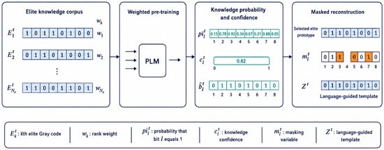
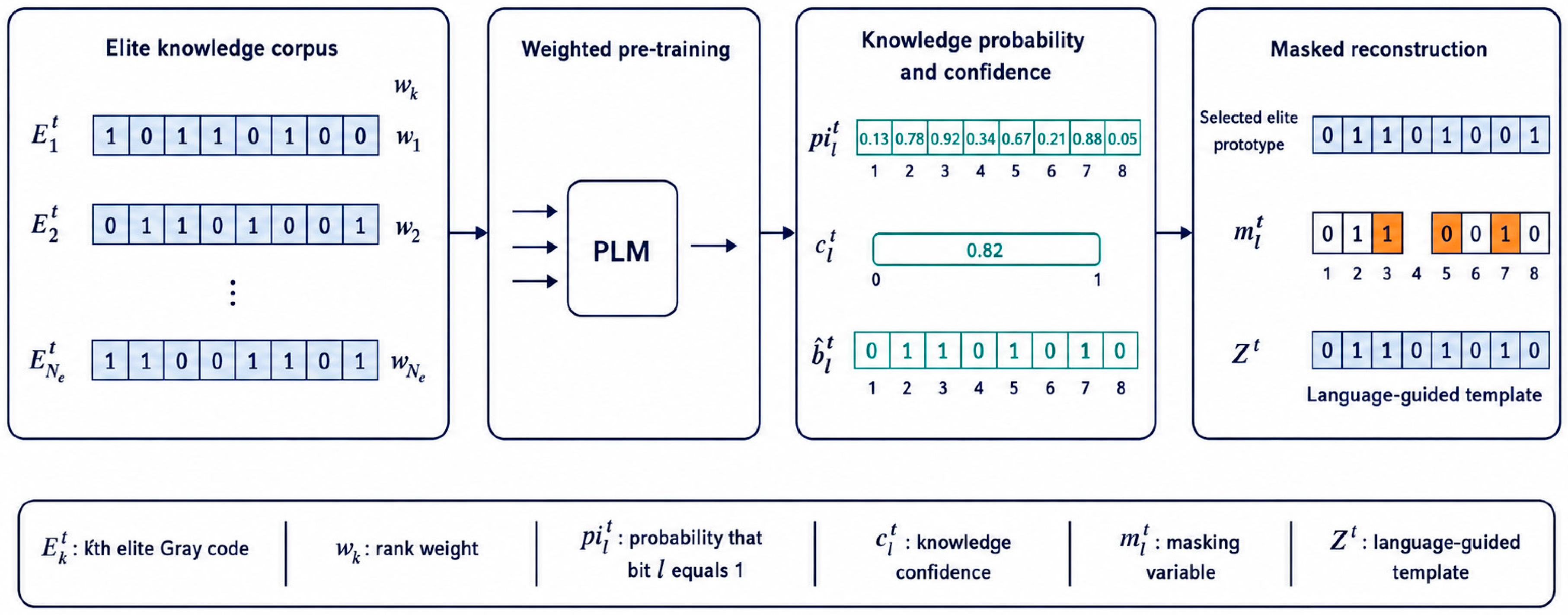
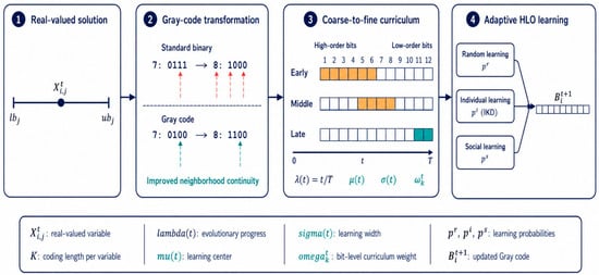
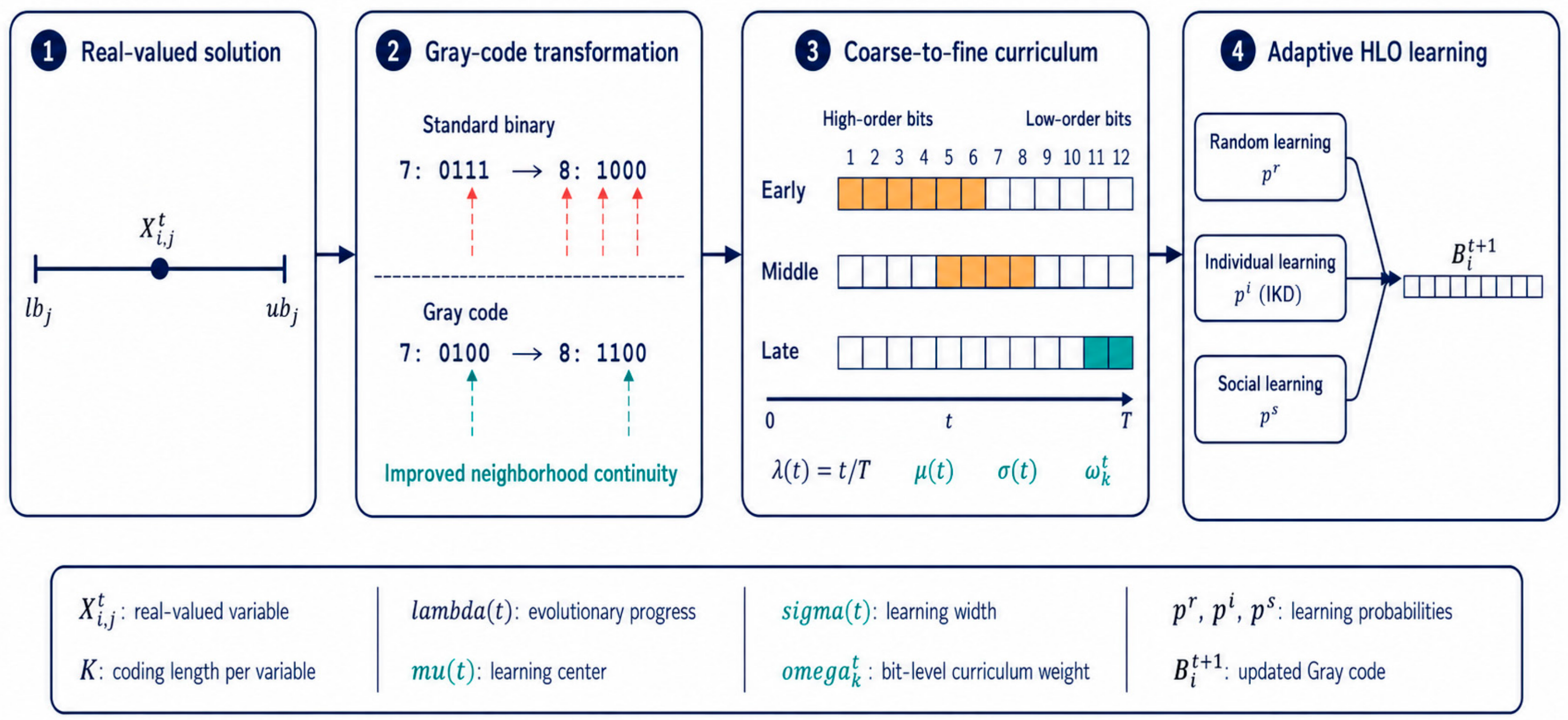
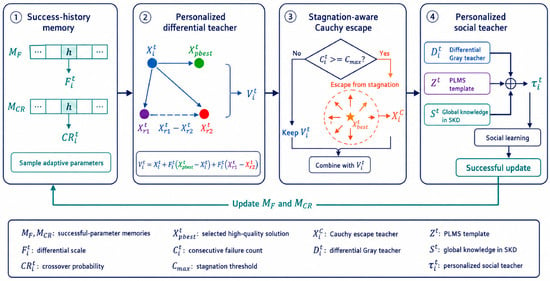
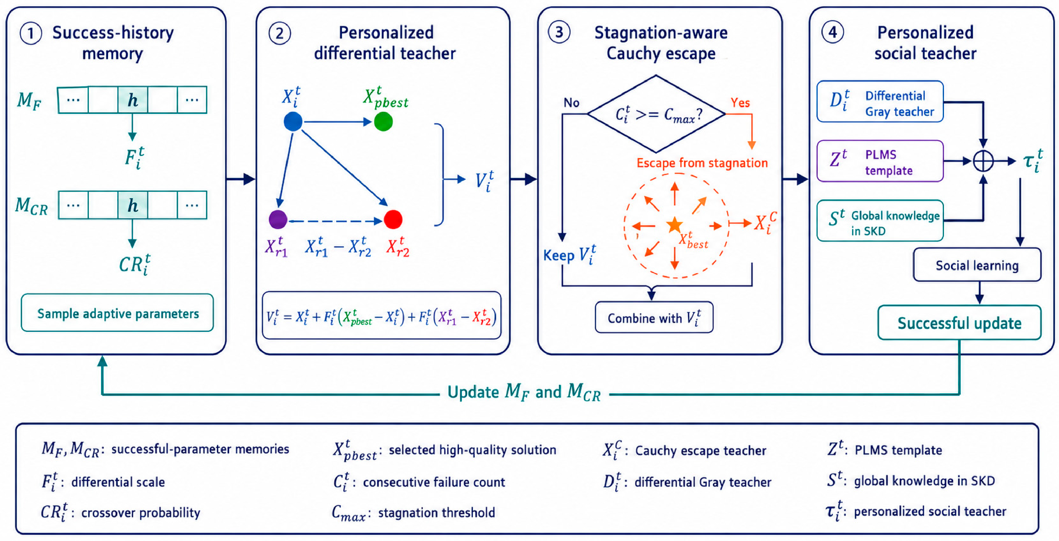
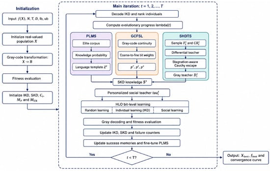
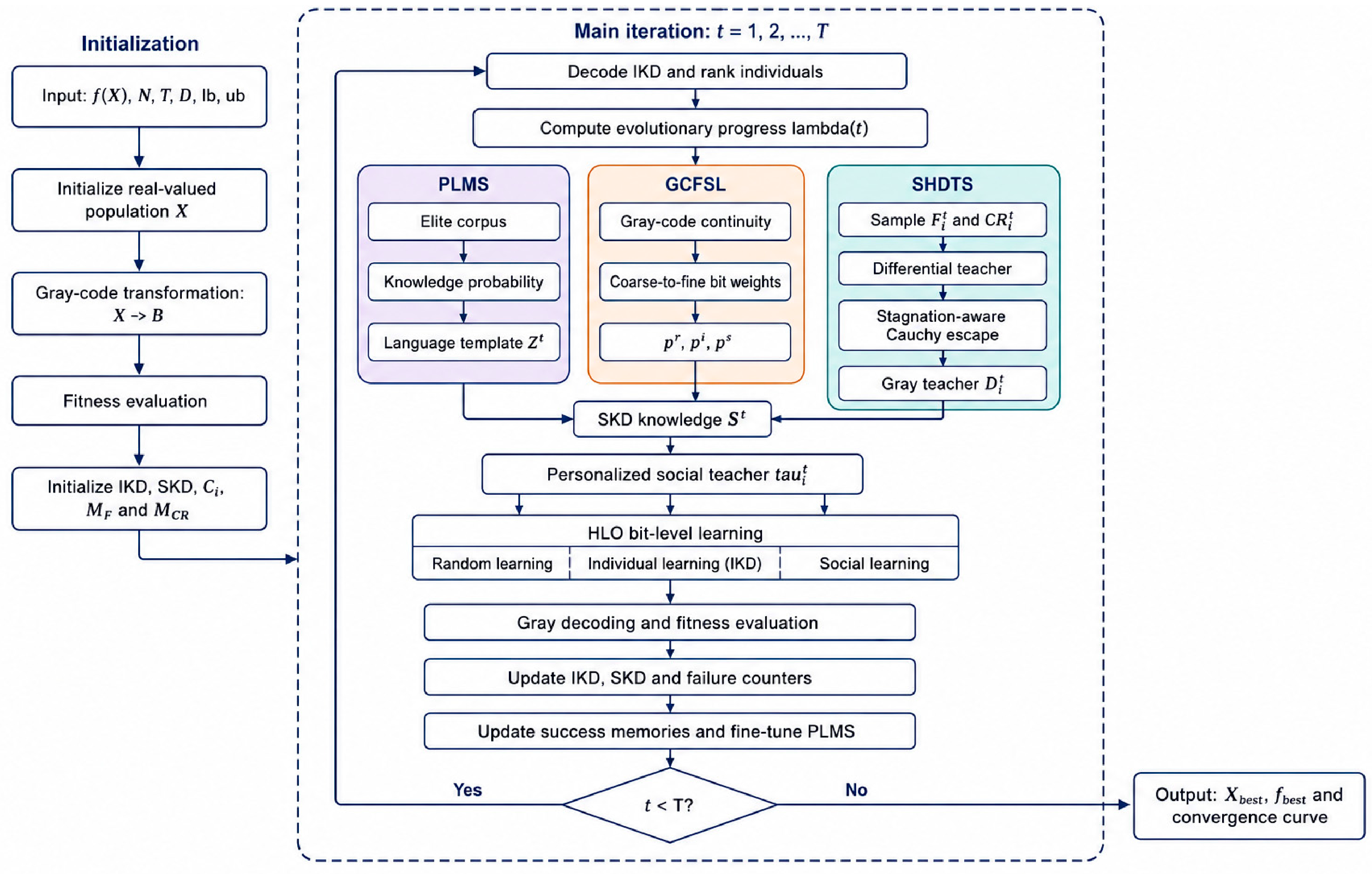
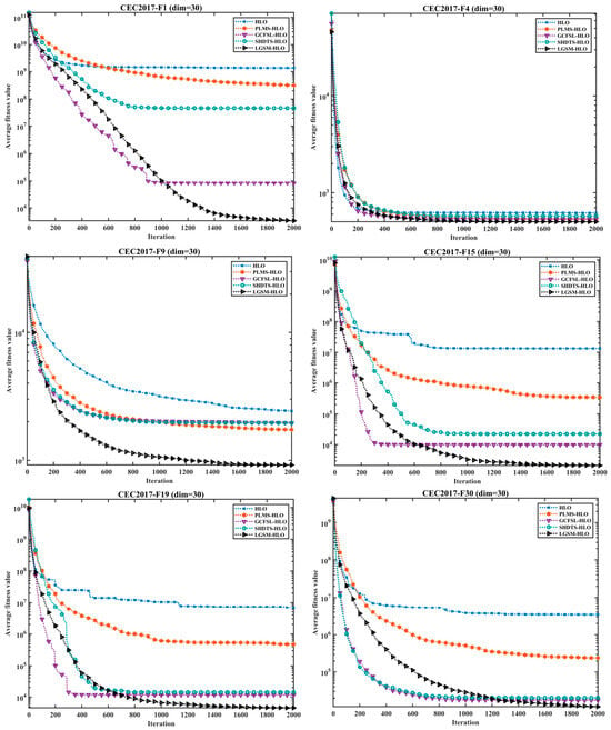
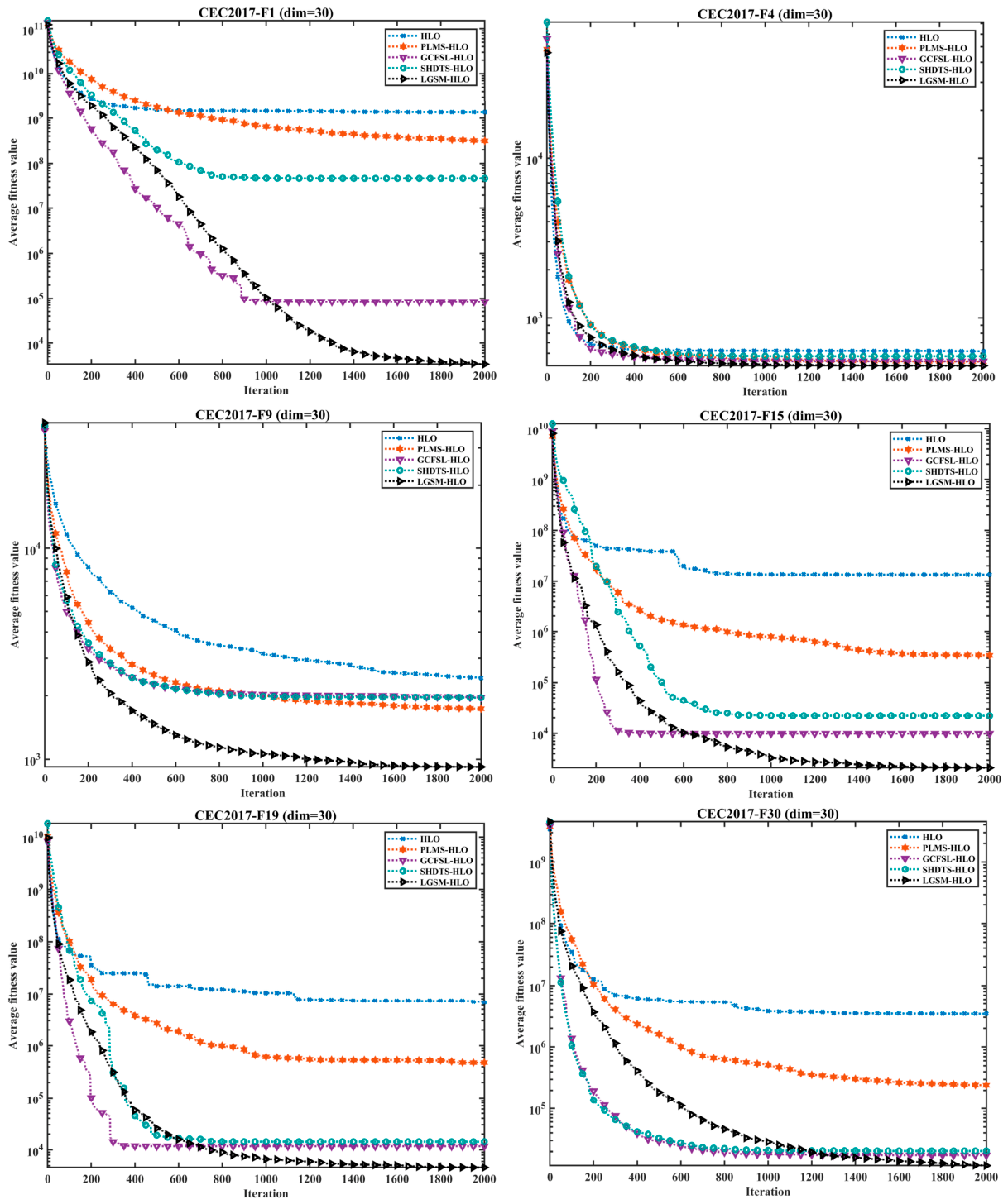
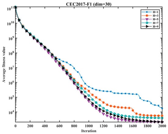
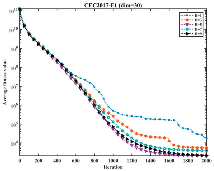
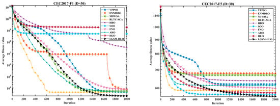
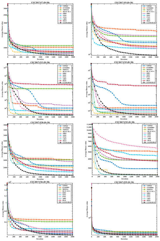
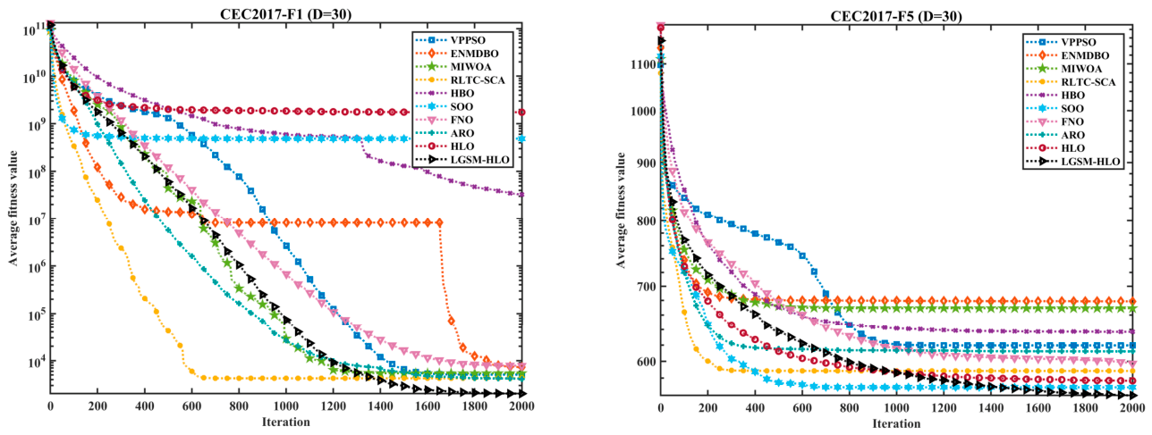
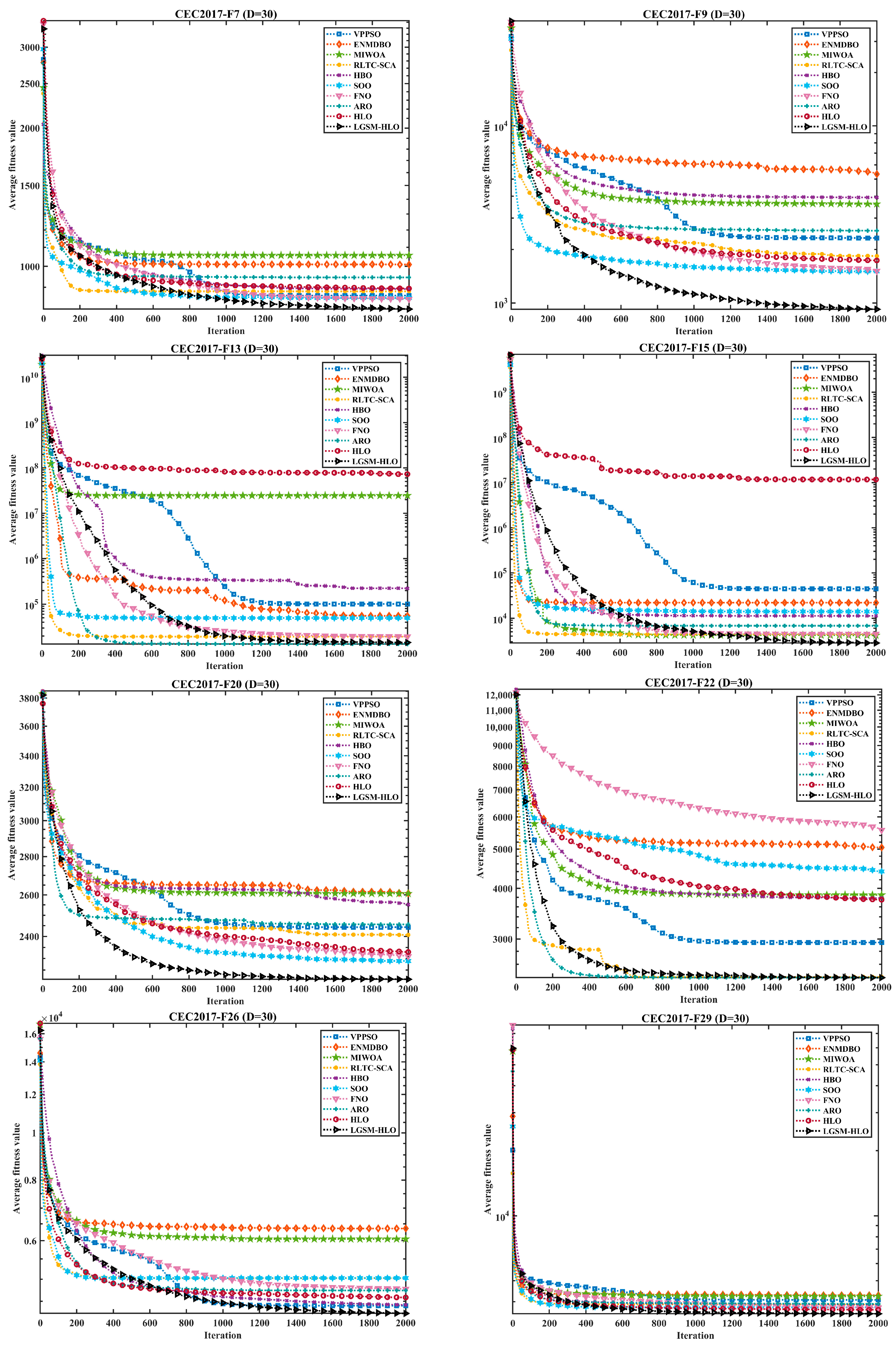
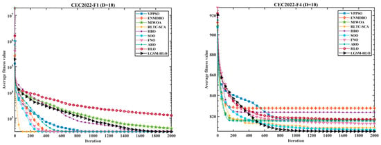
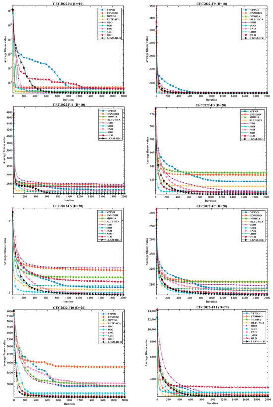
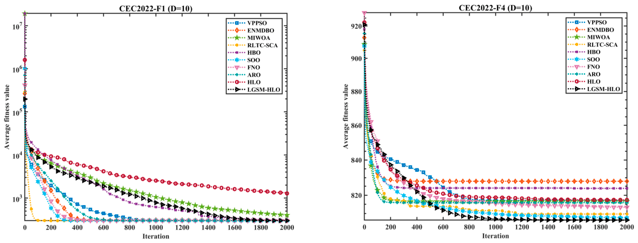
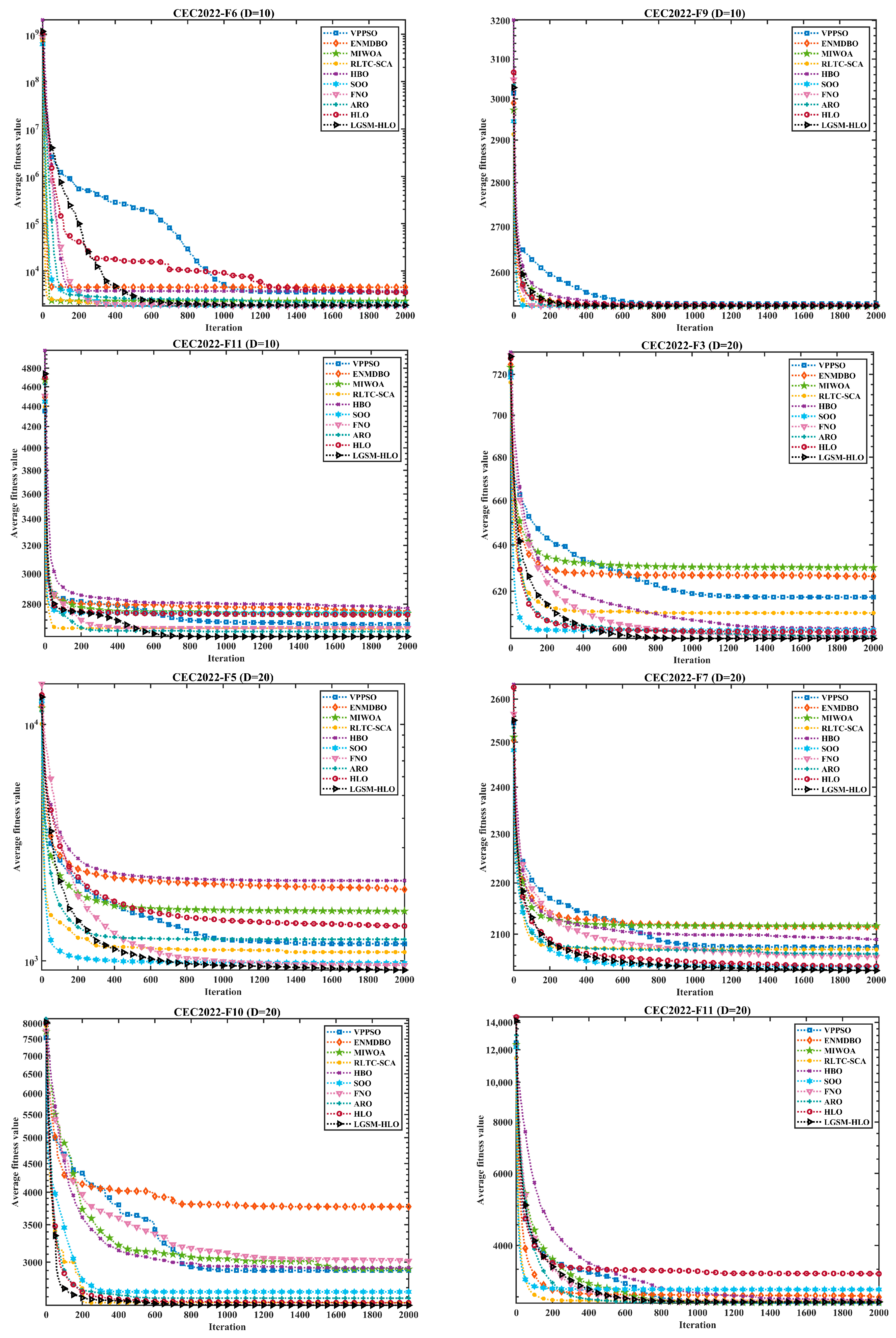
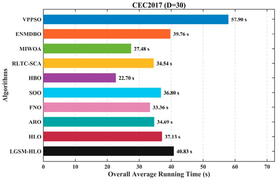
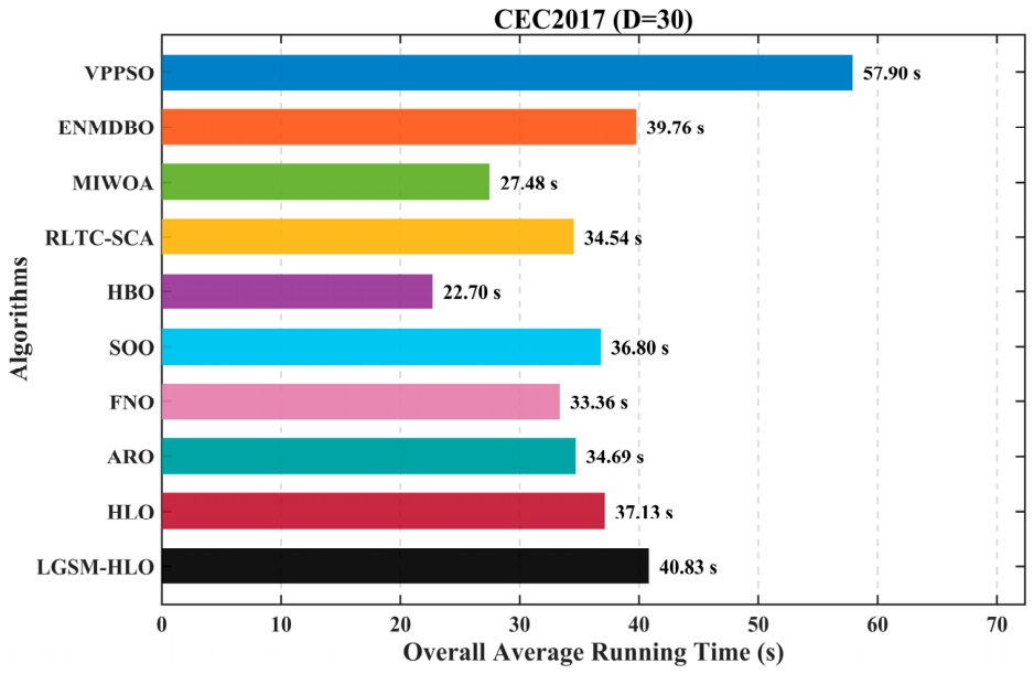
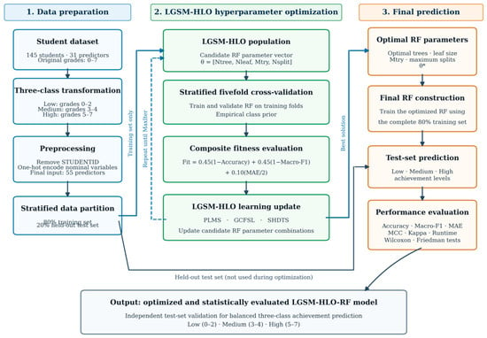
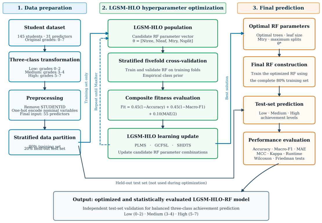
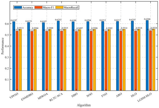
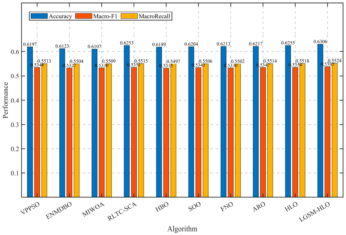

Disclaimer/Publisher’s Note: The statements, opinions and data contained in all publications are solely those of the individual author(s) and contributor(s) and not of MDPI and/or the editor(s). MDPI and/or the editor(s) disclaim responsibility for any injury to people or property resulting from any ideas, methods, instructions or products referred to in the content. |
© 2026 by the authors. Licensee MDPI, Basel, Switzerland. This article is an open access article distributed under the terms and conditions of the Creative Commons Attribution (CC BY) license.