Coordinated Economic Dispatch of Grid-Connected Microgrids Using an Asymmetric GE-RTH-SH Framework

Abstract

This study focuses on the single-objective day-ahead economic dispatch of grid-connected microgrids. It proposes an asymmetric GE-RTH-SH framework that integrates gradient-guided elite search (GE), Red-Tailed Hawk Optimization (RTH), and SHADE-lite adaptive differential search (SH). Based on the three-stage search mechanism of RTH (high-altitude circling, low-altitude circling, and dive hunting), GE local fine search and SH adaptive differential search based on successful history are introduced to improve local optimization accuracy and parameter adaptability and alleviate search stagnation. An aggregated microgrid model with a 24 h scheduling cycle and a 1 h time resolution is constructed to coordinate wind power, photovoltaic power, micro gas turbines, fuel cells, energy storage, and power exchange with the grid. The model is implemented in Python, aiming to minimize operation and maintenance costs, fuel costs, and net grid transaction costs, while satisfying power balance, equipment output, ramping, energy storage state of charge (SOC), and grid power exchange constraints. With a budget of 30,000 function evaluations per run, the average cost of 50 independent runs is CNY 5295.06, the standard deviation is 10.01, the best cost is CNY 5269.11, and the average renewable energy supply ratio is 62.55%. Through benchmark-function and ablation experiments, the search effects of the GE and SH modules are analyzed, and the optimization performance, economic performance, and repeatability of the complete algorithm are evaluated through comparisons with other algorithms in the microgrid case and four moderate disturbance scenarios. The results show that the proposed method can provide a feasible optimization scheme for coordinated power allocation and economic operation of grid-connected microgrids.

1. Introduction

As the application of renewable energy sources such as wind power and photovoltaic power in the distribution system continues to increase, the coordinated operation of distributed power sources and energy storage devices has gradually become an important aspect of microgrid research [1,2]. A microgrid (MG) organizes distributed power generation, energy storage, loads, and related control equipment within a single operating system and can conduct power exchange with the upstream power grid according to actual needs [3]. However, the output of wind power and photovoltaic (PV) power is greatly affected by meteorological conditions, and load demand and time-of-use electricity prices also change over time, causing microgrids to face different supply-demand relationships and economic conditions in different operating periods. Therefore, how to reasonably allocate the output of various power sources, the charging and discharging power of energy storage, and the power exchanged with the grid under the premise of meeting power supply safety and equipment operation constraints is the main problem that microgrid real-time economic dispatch needs to solve [4,5,6].

The economic dispatch of microgrids needs to take into account various conditions such as the output range of different power sources, power balance, ramp rate, energy storage state of charge (SOC), and grid connection power limit. The operation decisions for each period are also influenced by the states of previous and subsequent periods [6,7,8]. For models with clear mathematical expressions and the ability to be linearized or convexified, linear programming, mixed integer programming, and nonlinear programming methods usually provide more effective solution approaches. However, when the model contains non-convex characteristics, discrete operation conditions, or strong variable coupling relationships, the difficulty of solving also increases accordingly. Swarm intelligence and evolutionary optimization algorithms have relatively fewer requirements for the mathematical form of the objective function, and thus are widely used for approximate solutions to complex microgrid dispatch problems [8,9]. However, the solution effectiveness of these methods is still affected by the search strategy and parameter settings. How to balance the search range and the final solution accuracy remains a problem that needs to be addressed in the application of the algorithms.

The Red-Tailed Hawk Optimization algorithm (RTH), proposed by Ferahtia et al. in 2023, models three hunting stages—high-altitude circling, low-altitude circling, and diving—to balance exploration and exploitation in the search space [10]. Although RTH has a simple structure, like other swarm-based methods, it can suffer from rapid population aggregation, insufficient local exploitation, and search stagnation in complex multimodal or high-dimensional problems. Previous studies have introduced multi-strategy improvements or applied RTH to engineering problems such as optimal power flow, indicating the potential value of adaptive enhancement of its search mechanism [11,12].

In response to problems such as population aggregation, insufficient local search, and search stagnation that may occur in the basic RTH in complex search spaces, this paper retains its original three-stage search structure and introduces gradient-guided elite search and SHADE-lite adaptive differential search to construct the GE-RTH-SH algorithm. The two improvement strategies undertake different search tasks: The gradient-guided elite search utilizes the information of the target function’s variation near the candidate solutions to make local adjustments to the individuals with better fitness; SHADE-lite combines historical successful parameters and external archives to form the search direction of differential search, in order to alleviate the impact of premature concentration of the population. On this basis, a 24 h grid-connected microgrid operation model including wind power, photovoltaic power, micro gas turbines, fuel cells, energy storage systems, and the grid interaction is established. The single optimization objective is to minimize the total operation cost, and the proportion of renewable energy supply is used as an auxiliary evaluation indicator. The search performance of the algorithm is compared through standard test functions, and ablation experiments are set up to analyze the individual contributions of the two improvement strategies to the solution results.

2. Coordinated Economic Dispatch Model for Grid-Connected Microgrids

2.1. Basic Structure of the Microgrid

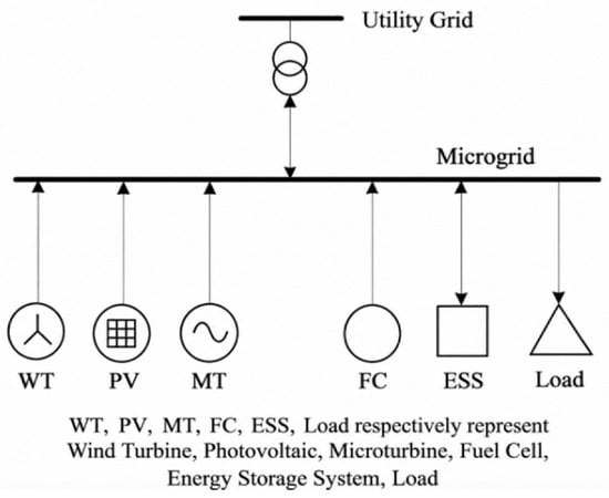
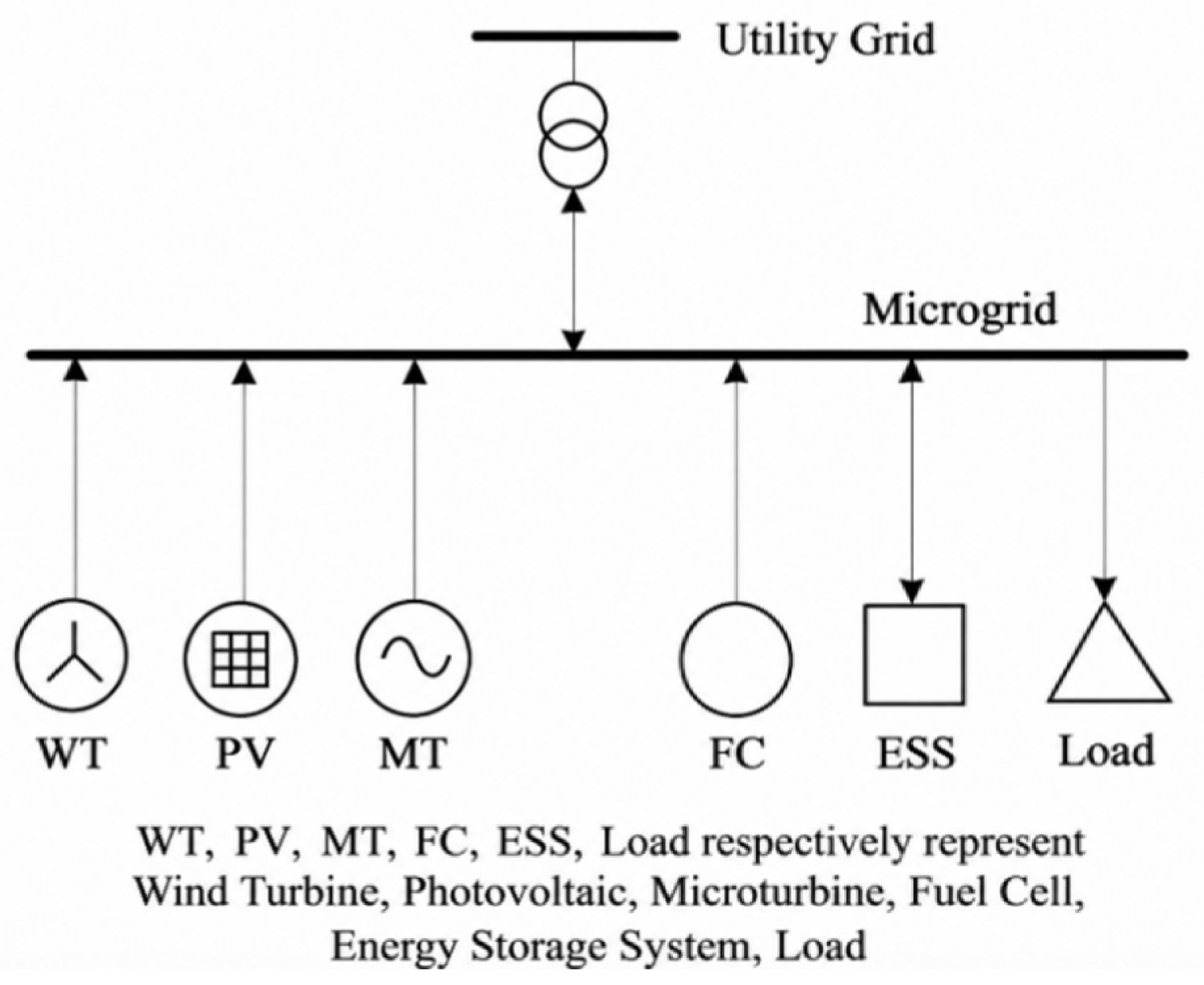
The structure of the grid-connected microgrid studied in this paper is shown in Figure 1. The system consists of wind turbines (WTs), photovoltaic units (PVs), micro gas turbines (MTs), fuel cells (FCs), energy storage system (ESS), electrical loads, and the public grid. Among them, the available power of wind and solar energy is affected by wind speed and solar irradiation conditions, respectively; the micro gas turbine and fuel cell, as dispatchable power sources, adjust their output power according to operational requirements; the energy storage system realizes the time transfer of electrical energy through charging and discharging at different times. The basic structure and grid-connected operation mode of the system refer to the framework described in Reference [3].

Figure 1. Schematic structure of the grid-connected microgrid.

The microgrid exchanges electrical energy with the higher-level power grid through the common connection point. When local power generation and energy storage discharge cannot meet the load demand, or when external purchased power has economic advantages, the system can purchase power from the main grid. When local power generation exceeds the load demand and meets the grid connection conditions, the excess power can be sold to the main grid. This paper does not involve equipment capacity configuration. The rated capacities of all equipment are regarded as known conditions. The main research focuses on the coordinated allocation among the output of distributed power sources, energy storage charging and discharging, and power purchase and sale of the grid within 24 h.

2.2. Economic Dispatch Objective Function

This paper aims to minimize the total operating cost over a 24 h period. The total cost includes the operation and maintenance costs of the power generation units, the operation and maintenance costs of the energy storage system, the fuel costs of the micro gas turbines and fuel cells, as well as the net expenditure resulting from electricity trading with the main power grid [11,12]. Related formulations of microgrid economic operation can be found in [13,14,15].

minC_total = C_OM + C_ESS + C_fuel + C_buy − C_sell  

(1)

where C_total represents the total operating cost over a 24 h scheduling period; C_om represents the operation and maintenance costs of each power generation unit; C_ESS represents the operation and maintenance costs of the energy storage system; C_fuel represents the fuel costs of the micro gas turbine and fuel cell; C_buy and C_sell, respectively, represent the costs incurred from purchasing electricity from the main grid and the revenues obtained from selling electricity to the main grid. This paper adopts 24 h as the complete scheduling period, with each scheduling period being 1 h, and there are a total of 24 periods.

2.2.1. Operation and Maintenance Cost

The proportional operation and maintenance as well as fuel cost expressions in formulas (2)–(8) of the microgrid dispatch model adopted in this paper adopt the simplified dispatch cost framework and original parameters as described in reference [9], and refer to the application dispatch studies in references [6,13,14,15].

The O&M cost of each generation unit is assumed to be proportional to its actual energy output and is expressed as follows:

$$C_{\mathrm{om}}={\displaystyle \sum _{t=1}^T}{\displaystyle \sum _{i=1}^{N_G}}{c}_{\mathrm{om},i}{P}_i\left(t\right)\Delta t$$

(2)

where N_G is the number of micro-sources included in the O&M cost calculation; P_i(t) is the output power of the i-th micro-source at time t; and c_om,i is the corresponding O&M cost coefficient per unit of energy.

2.2.2. Energy Storage O&M Cost

During the charging and discharging process of the energy storage system, certain operating and maintenance costs will be incurred. This article assumes that these costs are proportional to the total charging and discharging electricity of the energy storage system. The calculation formula is as follows:

$$C_{\mathit{ESS}}=c_{\mathit{ESS}}{\displaystyle \sum _{t=1}^T}(P_{\mathit{ch},t}+P_{\mathit{dis},t})\Delta t$$

(3)

where C_ESS is the total operating and maintenance cost of the energy storage system within a 24 h scheduling period; c_ESS is the operating and maintenance cost coefficient per unit of charging and discharging electricity of the energy storage system, which is set at 0.005 CNY/kWh; P_ch,t and P_dis,t represent the charging power and discharging power of the energy storage system in period t, both in kW; Δt is the scheduling period length, which is set at 1 h.

2.2.3. Fuel Cost

The microturbine and fuel cell consume fuel during power generation. Their total fuel cost is expressed as follows:

C_fuel = C_MT + C_FC 

(4)

$$C_{\mathrm{MT}}={\displaystyle \sum _{t=1}^T}{\displaystyle \frac{c_{\mathrm{MT}}{P}_{\mathrm{MT}}\left(t\right)\Delta t}{{\eta }_{\mathrm{MT}}{H}_{\mathrm{MT}}}}$$

(5)

$$C_{\mathrm{FC}}={\displaystyle \sum _{t=1}^T}{\displaystyle \frac{c_{\mathrm{FC}}{P}_{\mathrm{FC}}\left(t\right)\Delta t}{{\eta }_{\mathrm{FC}}{H}_{\mathrm{FC}}}}$$

(6)

where P_MT(t) and P_FC(t) represent the output power of the micro gas turbine and the fuel cell, respectively, in the corresponding time period; η_MT and η_FC are the power generation efficiencies of these two types of equipment; H_MT and H_FC, respectively, indicate the lower calorific value of the fuel used; c_MT and c_FC are the unit prices of the corresponding fuels. When calculating the fuel cost, necessary unit conversions of the lower calorific value should be performed to ensure consistency with the units used for electric power, power generation volume, and fuel prices.

2.2.4. Electricity Purchase Cost

When local supply is insufficient or purchasing electricity from the utility grid is economically advantageous, the electricity purchase cost is:

$$C_{\mathrm{buy}}={\displaystyle \sum _{t=1}^T}{\lambda }_{\mathrm{buy}}\left(t\right)P_{\mathrm{buy}}\left(t\right)\Delta t$$

(7)

where λ_buy(t) is the purchase tariff at time t, and P_buy(t) is the purchased power at the corresponding time.

2.2.5. Electricity Sales Revenue

When local generation is surplus and grid-export conditions are satisfied, the revenue from electricity sales is:

$$C_{\mathrm{sell}}={\displaystyle \sum _{t=1}^T}{\lambda }_{\mathrm{sell}}\left(t\right)P_{\mathrm{sell}}\left(t\right)\Delta t$$

(8)

where λ_sell(t) is the selling tariff at time t, and P_sell(t) is the exported power at the corresponding time. By coordinating controllable generation, ESS operation, and grid exchange, the model minimizes the total operating cost over the 24 h horizon for the specified equipment capacities.

2.3. Renewable Energy Evaluation Indicator

In addition to minimizing the 24 h total operating cost, the renewable energy supply ratio is introduced as an auxiliary indicator to evaluate the contribution of renewable generation to the system energy supply under different dispatch strategies. This indicator does not enter the objective function and is used only for post-optimization analysis of the energy-supply structure.

Wind and PV generation are treated as renewable energy sources. To avoid double counting caused by ESS charging and discharging, the ESS is not considered a primary energy source in the denominator. The renewable energy supply ratio is defined as the energy generated by wind and PV over the scheduling horizon divided by the total primary energy supplied to the microgrid:

$$R_{\mathrm{RE}}={\displaystyle \frac{{\displaystyle {\sum }_{t=1}^T}\left[P_{\mathrm{WT}}\left(t\right)+P_{\mathrm{PV}}\left(t\right)\right]\Delta t}{{\displaystyle {\sum }_{t=1}^T}\left[P_{\mathrm{WT}}\left(t\right)+P_{\mathrm{PV}}\left(t\right)+P_{\mathrm{MT}}\left(t\right)+P_{\mathrm{FC}}\left(t\right)+P_{\mathrm{buy}}\left(t\right)\right]\Delta t}}\times 100\%$$

(9)

where R_RE is the renewable energy supply ratio; P_WT(t) and P_PV(t) are the actual WT and PV outputs at time t; P_MT(t) and P_FC(t) are the MT and FC outputs, respectively; and P_buy(t) is the power purchased from the utility grid. This indicator reflects the relative contribution of renewable energy to the primary energy supply structure.

2.4. Microgrid Operating Constraints

The microgrid dispatching scheme not only needs to meet the requirements of operating costs, but also must comply with the actual operating conditions of various equipment. The constraints set in this paper include the hourly power balance of the system, the limit on the available power of wind and solar power generation, the limit on the output and ramp rate of controllable power sources, the limit on the state of charge (SOC) of the energy storage system (ESS) and the charging and discharging power, as well as the power exchange limit with the main grid. These constraints jointly determine the feasible solution range of the dispatching model and are not involved in the solution process as additional optimization objectives.

2.4.1. Power Balance Constraint

At each scheduling interval, total supply must equal the load demand plus ESS charging and power exported to the grid:

P_WT(t) + P_PV(t) + P_MT(t) + P_FC(t) + P_dis(t) + P_buy(t) = P_L(t) + P_ch(t) + P_sell(t)

(10)

where P_L(t) is the load power at time t; P_ch(t) and P_dis(t) are the ESS charging and discharging powers, respectively; the remaining symbols are defined above.

2.4.2. Micro-Source Output and Ramp-Rate Constraints

The actual outputs of wind and PV generation cannot exceed the available powers determined by the meteorological conditions in each interval:

$$0\le P_{\mathrm{WT}}\left(t\right)\le P_{\mathrm{WT}}^{\mathrm{av}}\left(t\right), 0\le P_{\mathrm{PV}}\left(t\right)\le P_{\mathrm{PV}}^{\mathrm{av}}\left(t\right)$$

(11)

The outputs of the MT and FC are restricted to their respective minimum and maximum operating limits:

$$P_j^{\min }\le P_j\left(t\right)\le P_j^{\max }, j\in \{\mathrm{MT},\mathrm{FC}\}$$

(12)

To avoid power changes between adjacent intervals that exceed the physical capabilities of controllable sources, the following ramp-rate constraints are imposed:

$$-R_j^{\mathrm{down}}\Delta t\le P_j\left(t\right)-P_j\left(t-1\right)\le R_j^{\mathrm{up}}\Delta t, j\in \{\mathrm{MT},\mathrm{FC}\}$$

(13)

where $P_{\mathrm{WT}}^{\mathrm{av}}\left(t\right)$ and $P_{\mathrm{PV}}^{\mathrm{av}}\left(t\right)$ represent the available power of wind power and photovoltaic power in period t, respectively; $P_j^{\min }$ and $P_j^{\max }$ represent the minimum and maximum output power of controllable power source j, respectively; P_j(t) and P_j(t − 1) are the output power of this power source in period t and the previous period, respectively; $R_j^{\mathrm{up}}$ and $R_j^{\mathrm{down}}$ represent the corresponding upward and downward ramp rate limits, respectively; Δt is the scheduling time interval, which is set to 1 h. Here, j ∈ {MT, FC}, corresponding to micro gas turbines and fuel cells, respectively.

2.4.3. Energy Storage System Operating Constraints

The energy storage system regulates the distribution of electric energy at different times through the charging and discharging processes, and its state of charge changes with the charging and discharging amounts. Let E_ESS represent the rated energy capacity of the energy storage system, and η_ch and η_dis represent the charging efficiency and discharging efficiency, respectively. Considering the energy loss during the charging and discharging processes, the change in SOC between adjacent time periods is determined by the charging power, discharging power, and corresponding efficiencies, and the state update relationship is as follows:

$$\mathit{SOC}\left(t+1\right)=\mathit{SOC}\left(t\right)+{\displaystyle \frac{{\eta }_{\mathrm{ch}}{P}_{\mathrm{ch}}\left(t\right)\Delta t}{E_{\mathrm{ESS}}}}-{\displaystyle \frac{P_{\mathrm{dis}}\left(t\right)\Delta t}{{\eta }_{\mathrm{dis}}{E}_{\mathrm{ESS}}}}$$

(14)

To prevent overcharging or overdischarging, the ESS SOC is constrained by:

SOC_min ≤ SOC(t) ≤ SOC_max,  SOC_min = 0.2, SOC_max = 0.8

(15)

The ESS charging and discharging powers are limited by their rated values, and simultaneous charging and discharging are prohibited:

$${-\mathrm{P}}_{\mathrm{ch}}^{\max }\le P_{\mathit{ESS},t}\le P_{\mathit{dis}}^{\mathit{max}} \left\{\begin{array}{c}{P}_{\mathit{ch},\mathrm{t}}=\max \left(0,-P_{\mathit{ESS},t}\right)\\ P_{\mathit{dis},\mathrm{t}}=\max \left(0,P_{\mathit{ESS},t}\right)\end{array}\right. P_{\mathrm{ch}}\left(t\right)P_{\mathrm{dis}}\left(t\right)=0$$

(16)

The implementation of the energy storage complementary constraint is as follows: The source code optimization process utilizes a single signed battery power variable P_ESS,t. Positive values indicate discharge, and negative values indicate charging. And P_dis,t = max(P_ESS,t, 0) and P_ch,t = max(−P_ESS,t, 0) are defined, ensuring that charging and discharging do not occur simultaneously from the variable construction perspective.

Because a 24 h cyclic dispatch is considered, the initial SOC is set to 0.50 and the terminal SOC is required to return to the same level. This prevents the optimizer from artificially reducing the daily operating cost by depleting the initial stored energy:

SOC(0) = SOC(T) = 0.5 

(17)

The above constraints limit the SOC of the energy storage system within the specified range, and also require that the SOC be restored to its initial level at the end of the scheduling period to avoid artificially reducing the daily operating cost by consuming the initial stored energy.

2.4.4. Grid Power Exchange Constraints

Power exchanged between the microgrid and the utility grid is limited by the tie-line capacity, and simultaneous electricity purchase and sale are prohibited:

$$0\le P_{\mathrm{buy}}\left(t\right)\le P_{\mathrm{buy}}^{\max }, 0\le P_{\mathrm{sell}}\left(t\right)\le P_{\mathrm{sell}}^{\max }, P_{\mathrm{buy}}\left(t\right)P_{\mathrm{sell}}\left(t\right)=0$$

(18)

where $P_{\mathrm{buy}}^{\max }$ and $P_{\mathrm{sell}}^{\max }$ are the maximum allowable import and export powers of the microgrid, respectively.

In summary, the model minimizes the 24 h total operating cost subject to power-balance, distributed-generation, ESS, and grid-exchange constraints. The renewable energy supply ratio is reported only as an auxiliary indicator for comparing the contribution of renewable generation under different dispatch solutions.

3. Economic Dispatch Method Based on Improved RTH

3.1. RTH

The Red-Tailed Hawk Optimization algorithm (RTH), proposed by Ferahtia et al. in 2023, simulates three hunting stages—high-altitude circling, low-altitude circling, and diving—to perform global exploration and local exploitation in the search space [10]. Let the optimization dimension be D, the population size be N, and the position of the i-th individual at iteration t be X_i(t). The current best position and the population mean are denoted by X_best and X_mean, respectively.

3.1.1. High-Altitude Circling Phase

During high-altitude circling, RTH uses the current best position, population mean, Lévy flight, and a transition factor to conduct broad exploration. The position update is:

X(t) = X_best + [X_mean − X(t − 1)] ⋅ Levy(D) ⋅ TF(t)

(19)

The Lévy flight function is calculated according to the original RTH formulation:

$$\mathit{Levy}\left(D\right)=s{\displaystyle \frac{\mathit{\mu \sigma }}{{\left|\nu \right|}^{\beta -1}}}, s=0.01,\hspace{0.25em}\beta =1.5$$

(20)

The transition factor is defined as:

$$\mathit{TF}\left(t\right)=1+\sin \left(2.5+{\displaystyle \frac{t}{T_{\mathit{max}}}}\right)$$

(21)

where T_max is the maximum number of iterations, and μ and ν are random variables. Lévy perturbation enlarges the exploration range and helps reduce premature population concentration.

3.1.2. Low-Altitude Circling Phase

As the search becomes concentrated around promising regions, the hawks perform spiral low-altitude circling around the current best position. The update rule is:

X(t) = X_best + [x(t) + y(t)] · StepSize(t)
StepSize(t) = X(t) − X_mean

(22)

where x(t) and y(t) are directional coordinates determined by the radius and angular functions. Their search scale gradually decreases as the iterations proceed, thereby strengthening local exploitation. The detailed coordinate definitions and parameter settings follow the original RTH [10].

3.1.3. Diving Phase

During the diving phase, individuals perform intensified local search around the best position obtained so far:

X(t) = α(t)X_best + x(t)StepSize₁(t) + y(t)StepSize₂(t)

(23)

where

$$\begin{array}{ll}\mathit{StepSiz}{e}_1\left(t\right)& =X\left(t\right)-\mathit{TF}\left(t\right)X_{\mathit{mean}}\\ \mathit{StepSiz}{e}_2\left(t\right)& =G\left(t\right)X\left(t\right)-\mathit{TF}\left(t\right)X_{\mathit{best}}\end{array}$$

(24)

$$\alpha \left(t\right)={\sin }^2\left(2.5-{\displaystyle \frac{t}{T_{\mathit{max}}}}\right), G\left(t\right)=2\left(1-{\displaystyle \frac{t}{T_{\mathit{max}}}}\right)$$

(25)

Through these three stages, RTH maintains a broad exploration range during the early search and gradually strengthens exploitation around promising regions in later iterations. The improvements introduced below retain this three-stage RTH framework [10,11,12].

3.2. GE-RTH-SH: An Asymmetric Complementary Search Framework

The basic RTH completes the search through three stages of position updates. However, in complex multi-modal problems, the population may gradually concentrate in a local area, resulting in insufficient subsequent search directions and making it difficult to further improve the existing optimal solutions. To address this issue, this paper retains the original search framework of RTH and adds two modules on its basis: the gradient-guided elite search and the SHADE-lite adaptive differential search. The former is mainly used to improve the local search near the optimal solution, while the latter provides more candidate search directions for the population by adjusting the differential search parameters and introducing external archives.

3.2.1. Gradient-Guided Elite Search

In each generation of the population, the individuals with the best fitness are selected for gradient-guided local search [16]. Based on the direction of change in the objective function near the current solution, the positions of the elite individuals are adjusted within a small range to further search for potentially better solutions in their neighboring areas. The specific update relationship is as follows:

θ_new = θ_old − η∇J(θ_old)

(26)

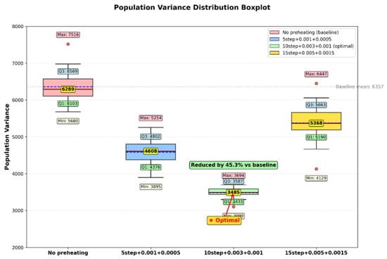
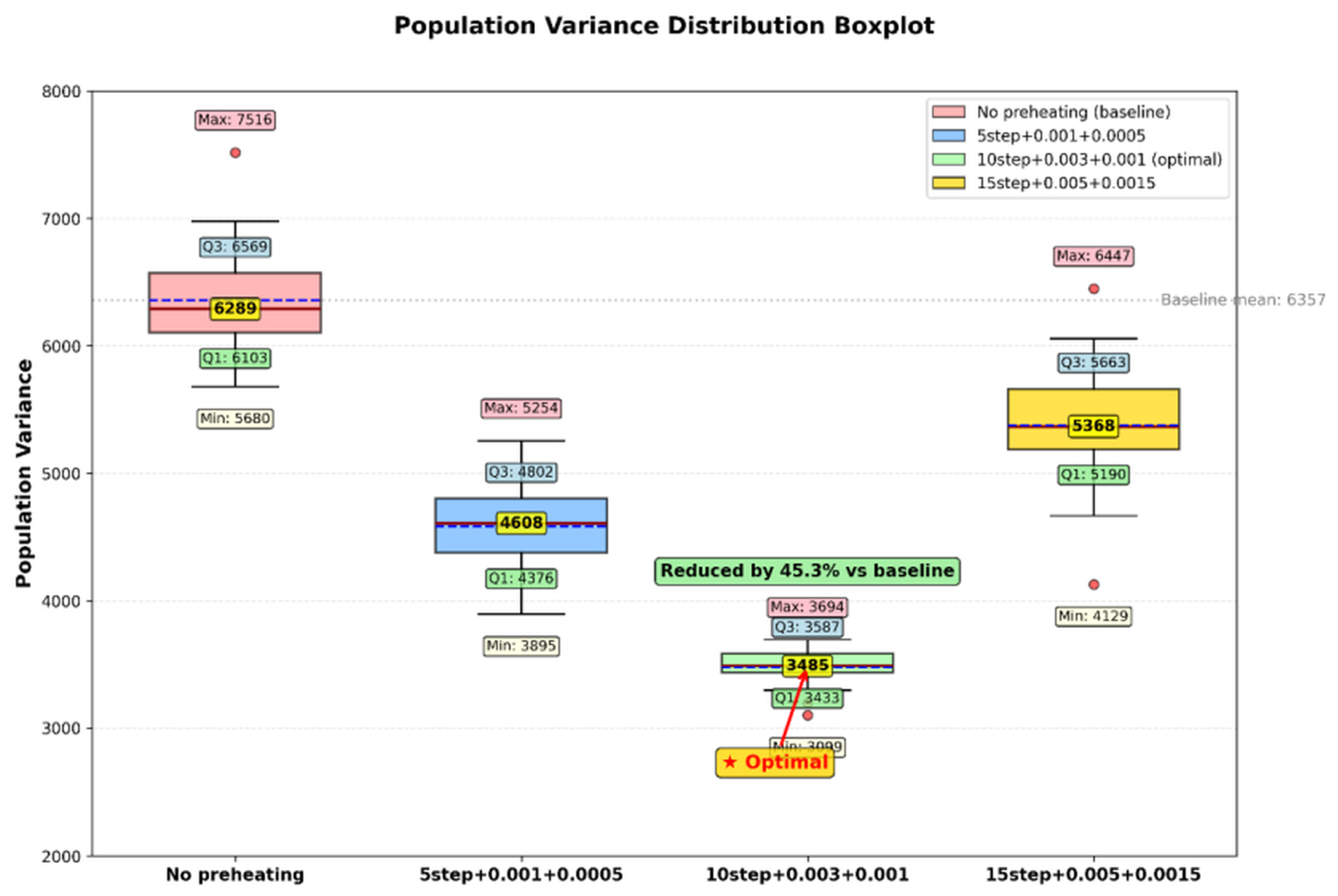
where θ is the decision vector to be optimized, J is the objective function, and η is the local-search step size. Unlike the learning-rate warm-up mechanism used in neural-network training, the step-size parameter here controls the magnitude of local perturbations during optimization. A relatively small step is used initially to avoid moving elite individuals too far from promising regions, after which the search scale is adjusted according to the preset schedule. When an analytical gradient is unavailable, a central-difference approximation is used, and the associated function evaluations are counted in the MaxFEs budget. A three-factor, three-level orthogonal experiment was conducted to assess the number of local-search steps, initial step size, and step-size increment. The setting of 10 local-search steps, an initial step size of 0.003, and an increment of 0.001 yielded the lowest population objective-function variance and the most concentrated outcomes, and was therefore adopted in the subsequent experiments. The fitness distribution for different gradient-guided parameter combinations is shown in Figure 2.

Figure 2. Fitness distribution for different gradient-guided parameter combinations.

3.2.2. SHADE-Lite Success-History-Based Adaptive Differential Search

To mitigate population clustering and limited search directions in the middle and late stages of RTH, a lightweight success-history-based adaptive differential search module is applied after the RTH position update. The mechanism is derived from differential evolution (DE) and SHADE [17,18]. Candidate vectors are generated using a current-to-pbest strategy:

$$v_i^t=x_i^t+F_i^t\left(x_{\mathit{pbest}}^t-x_i^t\right)+F_i^t\left(x_{r1}^t-x_{r2}^t\right)$$

(27)

where ${\mathrm{x}}_{\mathrm{pbest}}^{\mathrm{t}}$ is randomly selected from the top p% individuals of the current population; ${\mathrm{x}}_{\mathrm{r}1}^{\mathrm{t}}$ and ${\mathrm{x}}_{\mathrm{r}2}^{\mathrm{t}}$ are selected from the current population or the external archive; and ${\mathrm{F}}_{\mathrm{i}}^{\mathrm{t}}$ is the differential scaling factor.

The differential scaling factor F and crossover probability CR are sampled around the historical successful parameters as follows:

$$F_i^t\sim \mathit{Cauchy}\left(M_F,0.1\right), 0.05\le F_i^t\le 1$$

(28)

$$C{R}_i^t\sim N\left(M_{\mathit{CR}},0.1\right), 0\le C{R}_i^t\le 1$$

(29)

A trial vector is then generated through binomial crossover, followed by greedy selection to retain the better solution:

$$u_{\mathit{ij}}^t=\left\{\begin{array}{ll}{v}_{\mathit{ij}}^t,& {\mathit{rand}}_{\mathit{ij}}<C{R}_i^t\hspace{0.25em}\mathrm{or}\hspace{0.25em}j=j_{\mathit{rand}}\\ x_{\mathit{ij}}^t,& \mathrm{otherwise}\end{array}\right.$$

(30)

The F and CR values associated with successful updates are stored and used to update the historical memories, so that subsequent parameter distributions gradually shift toward regions that are more likely to produce high-quality solutions. The external archive stores replaced individuals and therefore provides additional difference directions when the population becomes highly concentrated, helping to preserve search diversity.

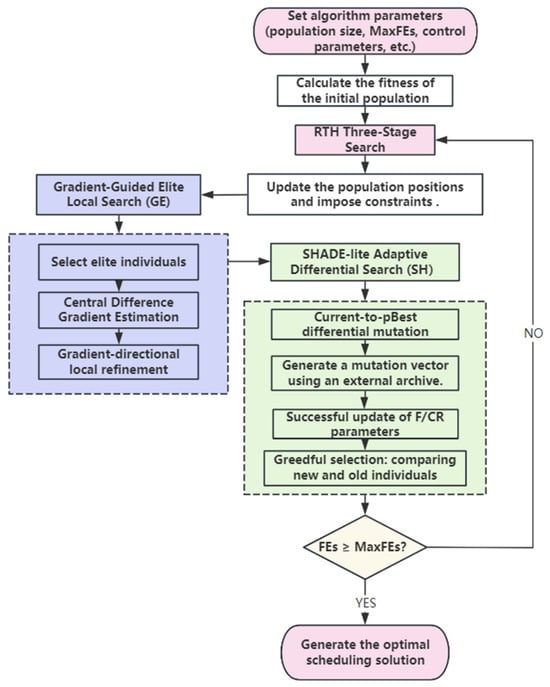
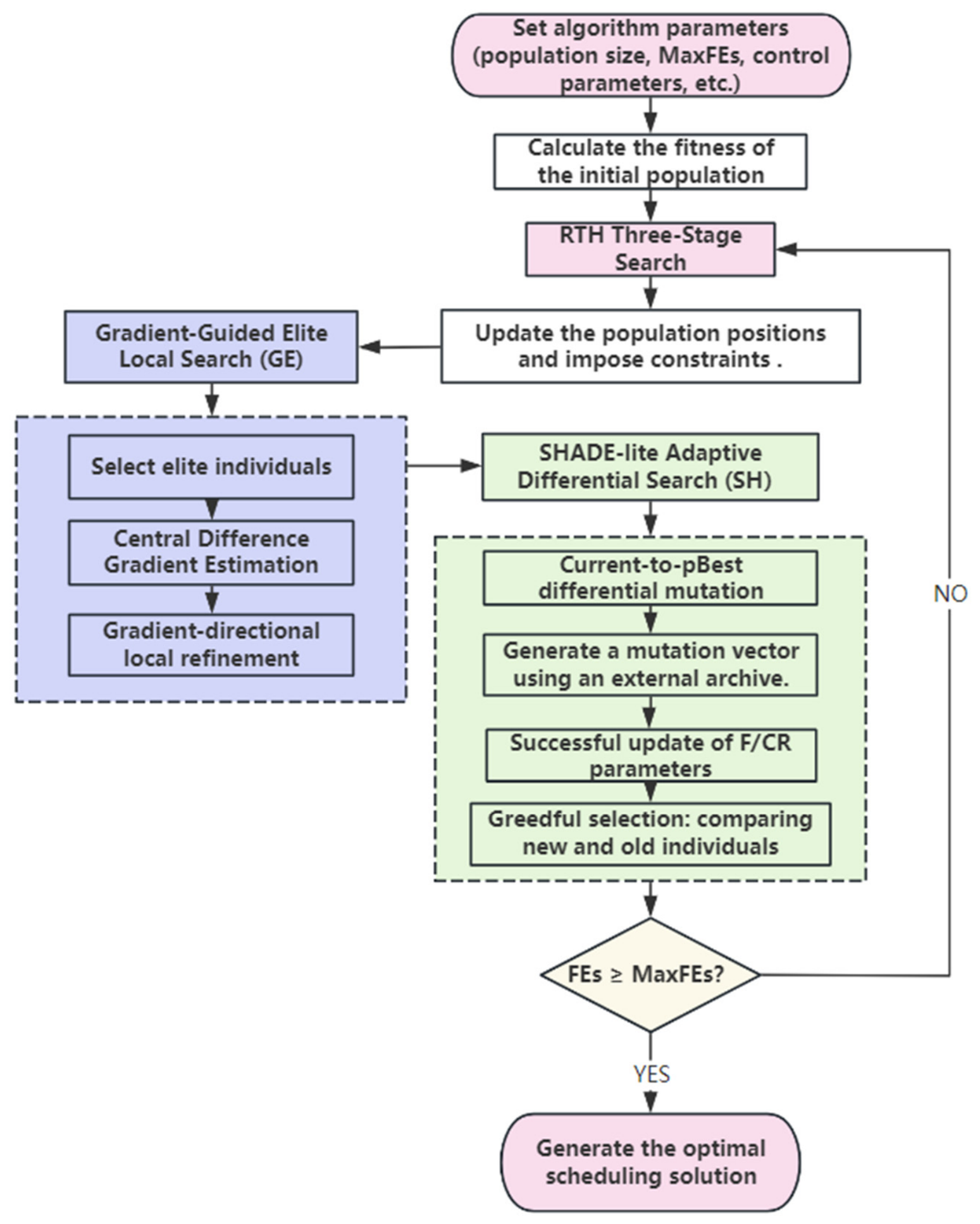
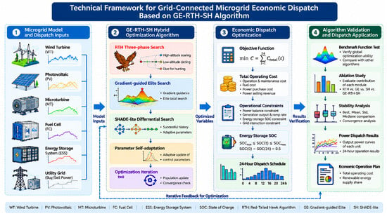
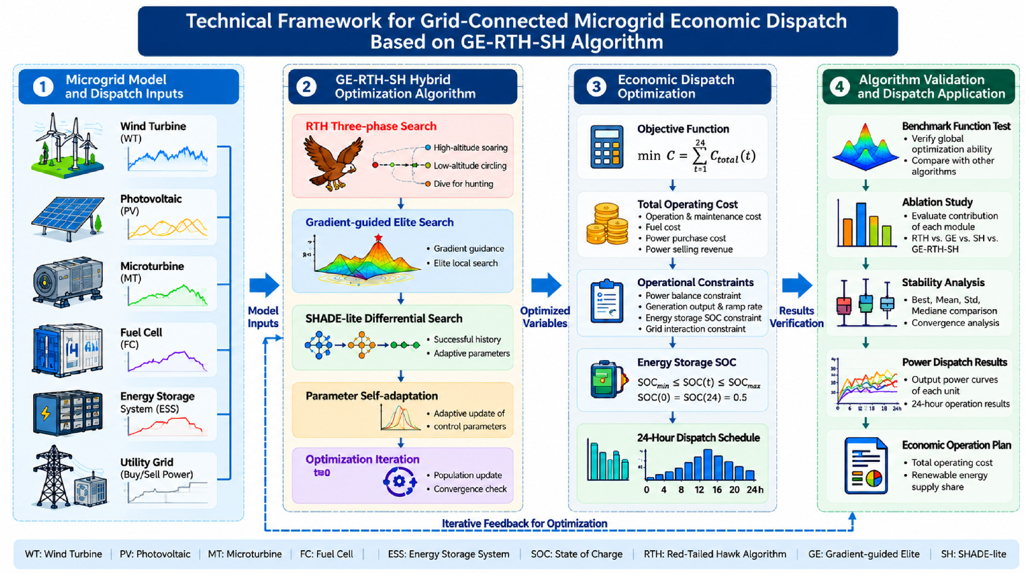
Considering that differential search will increase the number of evaluations of the objective function, this paper does not always execute the SHADE-lite module in each round of iteration. Instead, it decides whether to enable this module based on the problem dimension, the current search progress, and the continuous stagnation of the population. In this way, differential search is scheduled at the stage where additional search directions are needed to control its extra computational cost. The overall execution flow of the GE-RTH-SH algorithm is shown in Figure 3, and the relationship between the algorithm and the microgrid economic dispatch model is shown in Figure 4.

Figure 3. GE-RTH-SH optimization flowchart.

Figure 4. Overall framework of GE-RTH-SH-based microgrid economic dispatch.

GE-RTH-SH is based on the three-stage search of RTH and introduces local fine search and adaptive differential search during the population update process. The gradient-guided elite search focuses on adjusting the current superior individuals, while SHADE-lite utilizes historical successful parameters and external archives to generate new candidate solutions. The two mechanisms differ in the search object and update method, respectively addressing the issues of insufficient local improvement and restricted search direction of the population. The actual effect of their combination will be evaluated in subsequent standard function tests and microgrid scheduling examples.

3.3. Algorithm Performance Evaluation

To evaluate the search performance, PSO, WOA, GA, RTH and DBO were compared with GE-RTH-SH on classic standard test functions. Among them, the theoretical basis of the GA method is derived from the classic framework of genetic algorithms; the definition and range of the test functions are based on the review of standard test functions [19]. The selected functions include single-peak and multi-peak search spaces, which can be used to evaluate the local fine search and global exploration capabilities. The definitions and basic parameters of the benchmark functions are shown in Table 1.

Table 1. Definitions and basic parameters of the benchmark functions.

No.	Function	Expression	Dimension D	Search Range	Theoretical Optimum f*	Type
1	Sphere	Σxi2	30	[−100, 100]	0	Unimodal
2	Schwefel 2.21	Max|xi|	30	[−10, 10]	0	Unimodal
3	Schwefel 2.22	Σ|xi| + Π|xi|	30	[−10, 10]	0	Unimodal
4	Rosenbrock	Σ[100(xi+1 − xi2)2+(xi − 1)2]	30	[−30, 30]	0	Unimodal
5	Griewank	Σxi2/4000 − Πcos(xi/√i) + 1	30	[−600, 600]	0	Multimodal
6	Ackley	−20 exp[−0.2√(Σxi2/D)] − exp[Σcos(2πxi)/D] + 20 + e	30	[−32, 32]	0	Multimodal
7	Branin	(x2 − 5.1 × 12/(4π2) + 5 × 1/π − 6)2 + 10(1 − 1/(8π))cosx1 + 10	2	x1∈[−5, 10]; x2∈[0, 15]	0.397887	Multimodal
8	Rastrigin	Σ[xi2 − 10 cos(2πxi) + 10]	30	[−5.12, 5.12]	0	Multimodal

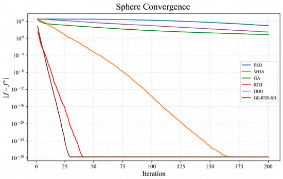
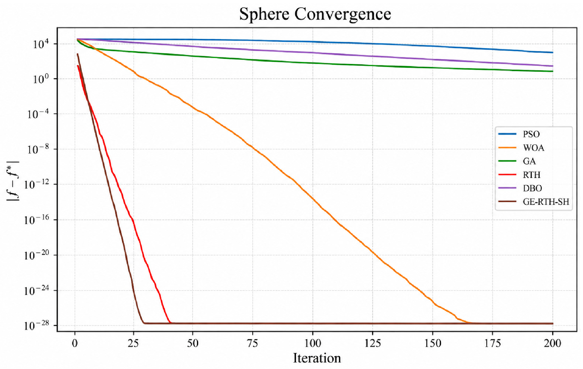
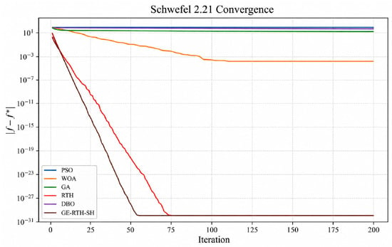
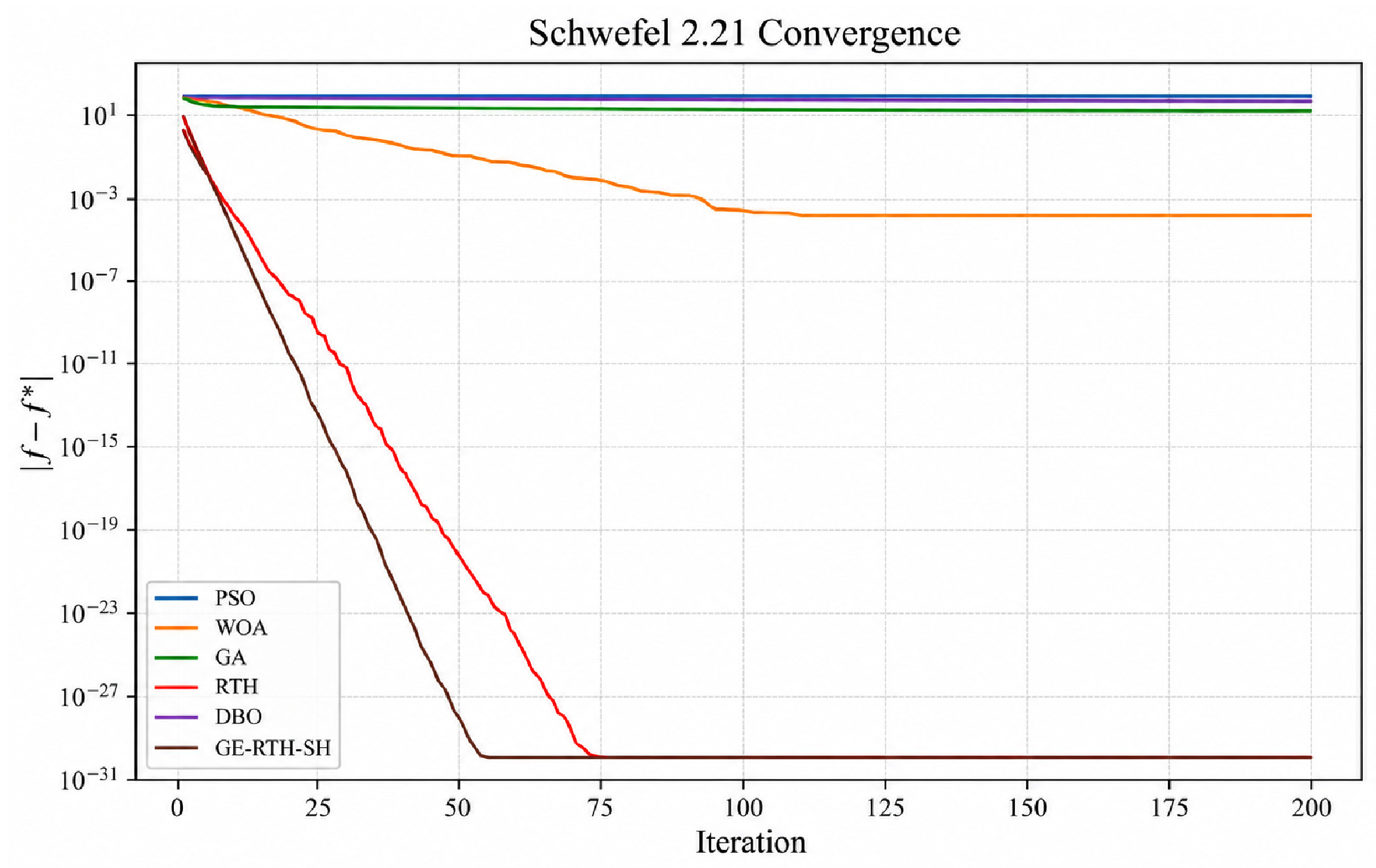
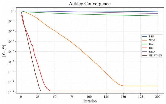
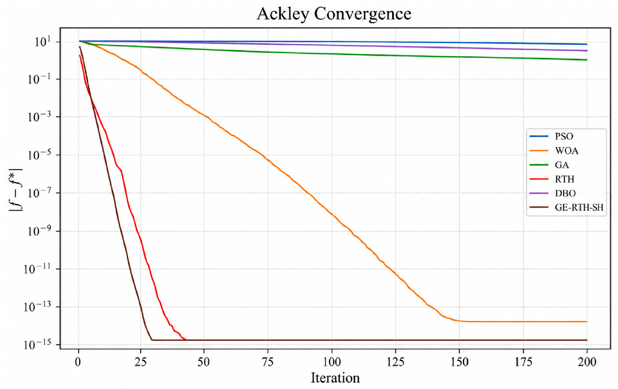
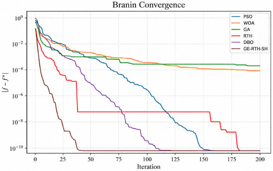
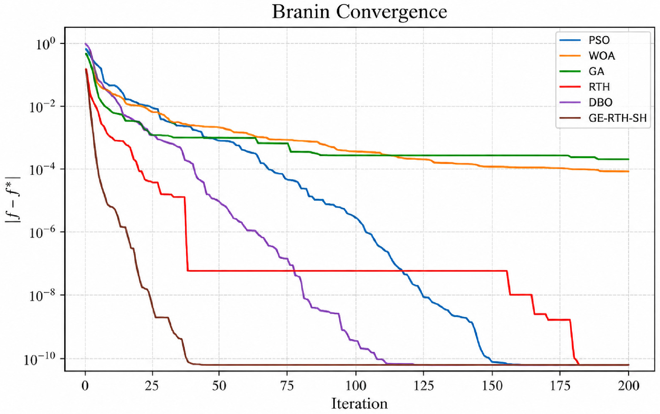
Table 2 summarizes the final solution results of each algorithm after 20 independent runs. Best, mean, and Std represent the optimal value, average value, and standard deviation, respectively. The convergence curves in Figure 5, Figure 6, Figure 7 and Figure 8 are plotted using the average historical best fitness values of each run at corresponding iteration stages. Therefore, the end points of the curves correspond to the average values of the final results of multiple runs, rather than the best values in Table 2. The benchmark results show that GE-RTH-SH achieves faster convergence and higher final solution accuracy than PSO, WOA, GA, RTH, and DBO on most of the reported functions. On unimodal functions such as Sphere and Schwefel 2.21, the proposed method rapidly approaches the theoretical optimum, indicating strong local exploitation. On multimodal functions such as Ackley, the convergence trajectory also decreases effectively, suggesting that the combined SHADE-lite differential search and gradient-guided elite search can help preserve population exploration, alleviate stagnation, and improve late-stage search accuracy. Overall, GE-RTH-SH maintains a useful balance between exploration and exploitation, providing a basis for its application to microgrid economic dispatch with coupled variables and operational constraints. The next section examines the individual contributions of the GE and SH components through ablation experiments.

Table 2. Summary of benchmark-function results.

Function	Algorithm	Mean	Best	Std
Ackley	DBO	6.202655	2.243784	4.698682
Ackley	GA	1.777956	9.882951 × 10−1	4.403599 × 10−1
Ackley	GE-RTH-SH	4.440892 × 10−16	4.440892 × 10−16	0.000000
Ackley	PSO	1.361166 × 101	5.647147	6.078590
Ackley	RTH	4.440892 × 10−16	4.440892 × 10−16	0.000000
Ackley	WOA	9.503509 × 10−15	3.996803 × 10−15	4.678548 × 10−15
Branin	DBO	3.978874 × 10−1	3.978874 × 10−1	0.000000
Branin	GA	3.980909 × 10−1	3.978874 × 10−1	6.146915 × 10−4
Branin	GE-RTH-SH	3.978874 × 10−1	3.978874 × 10−1	0.000000
Branin	PSO	3.978874 × 10−1	3.978874 × 10−1	0.000000
Branin	RTH	3.978874 × 10−1	3.978874 × 10−1	0.000000
Branin	WOA	3.979714 × 10−1	3.978874 × 10−1	2.847545 × 10−4
Schwefel 2.21	DBO	3.772816 × 101	2.555370 × 101	5.309821
Schwefel 2.21	GA	1.197225 × 101	7.743694	3.110851
Schwefel 2.21	GE-RTH-SH	7.159857 × 10−136	3.485253 × 10−142	2.391834 × 10−135
Schwefel 2.21	PSO	5.795180 × 101	4.675125 × 101	6.426180
Schwefel 2.21	RTH	2.172853 × 10−91	1.730882 × 10−98	6.489115 × 10−91
Schwefel 2.21	WOA	1.875147 × 10−4	6.004223 × 10−8	4.968460 × 10−4
Sphere	DBO	2.243284 × 101	4.009761	1.875633 × 101
Sphere	GA	5.255840	3.476421	1.363577
Sphere	GE-RTH-SH	7.974239 × 10−273	6.902948 × 10−285	0.000000
Sphere	PSO	1.260960 × 103	2.441538 × 102	2.318589 × 103
Sphere	RTH	1.910340 × 10−181	2.899494 × 10−194	0.000000
Sphere	WOA	2.316903 × 10−35	5.376765 × 10−38	6.474777 × 10−35

Figure 5. Sphere convergence test.

Figure 6. Schwefel 2.21 convergence test.

Figure 7. Ackley convergence test.

Figure 8. Branin convergence test.

3.4. Ablation Study and Computational Cost Analysis

3.4.1. Ablation Study

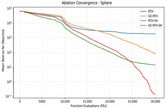
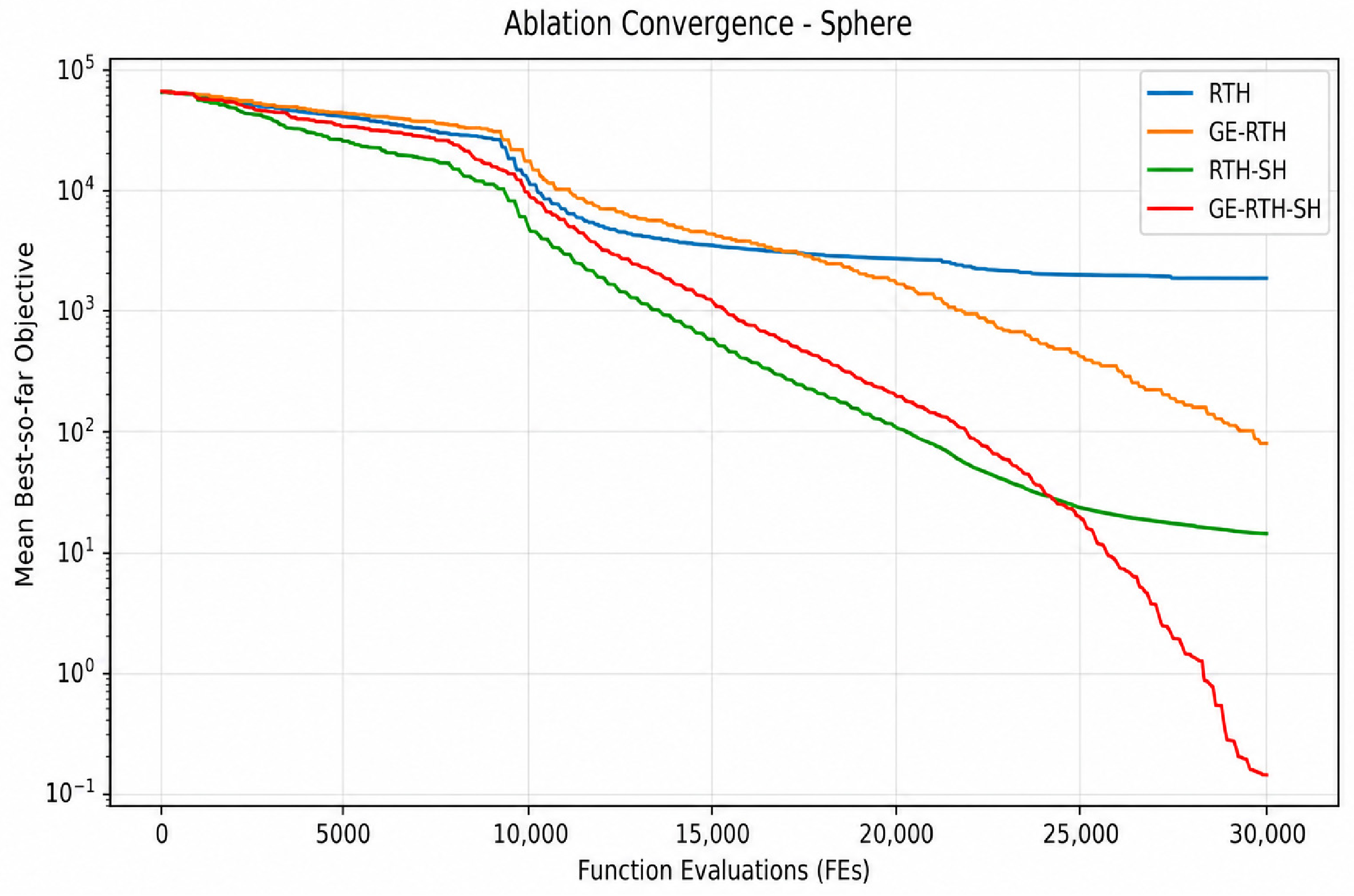
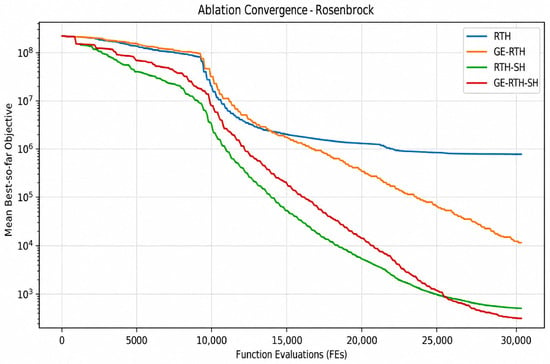
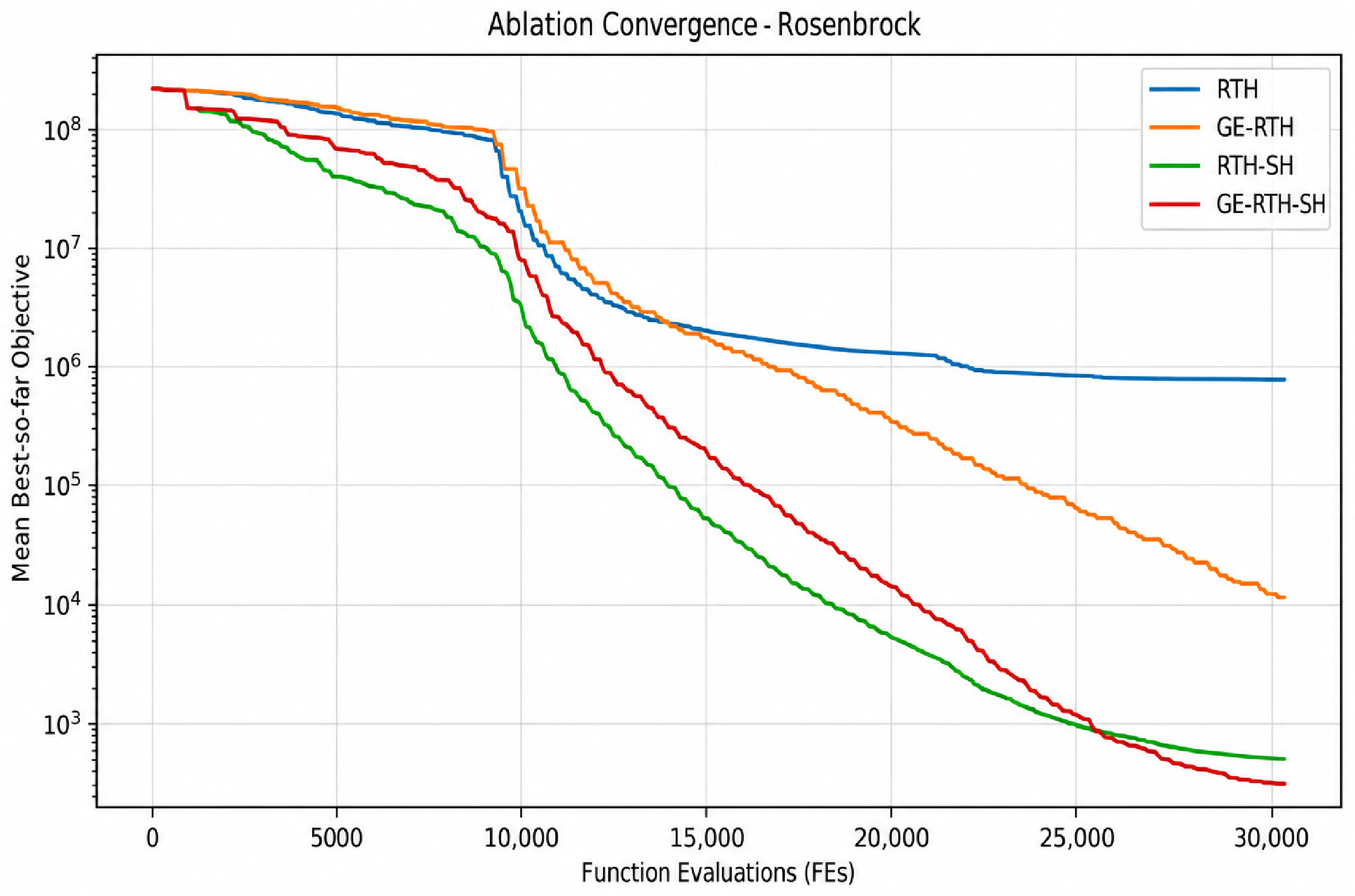
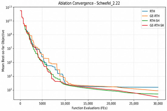
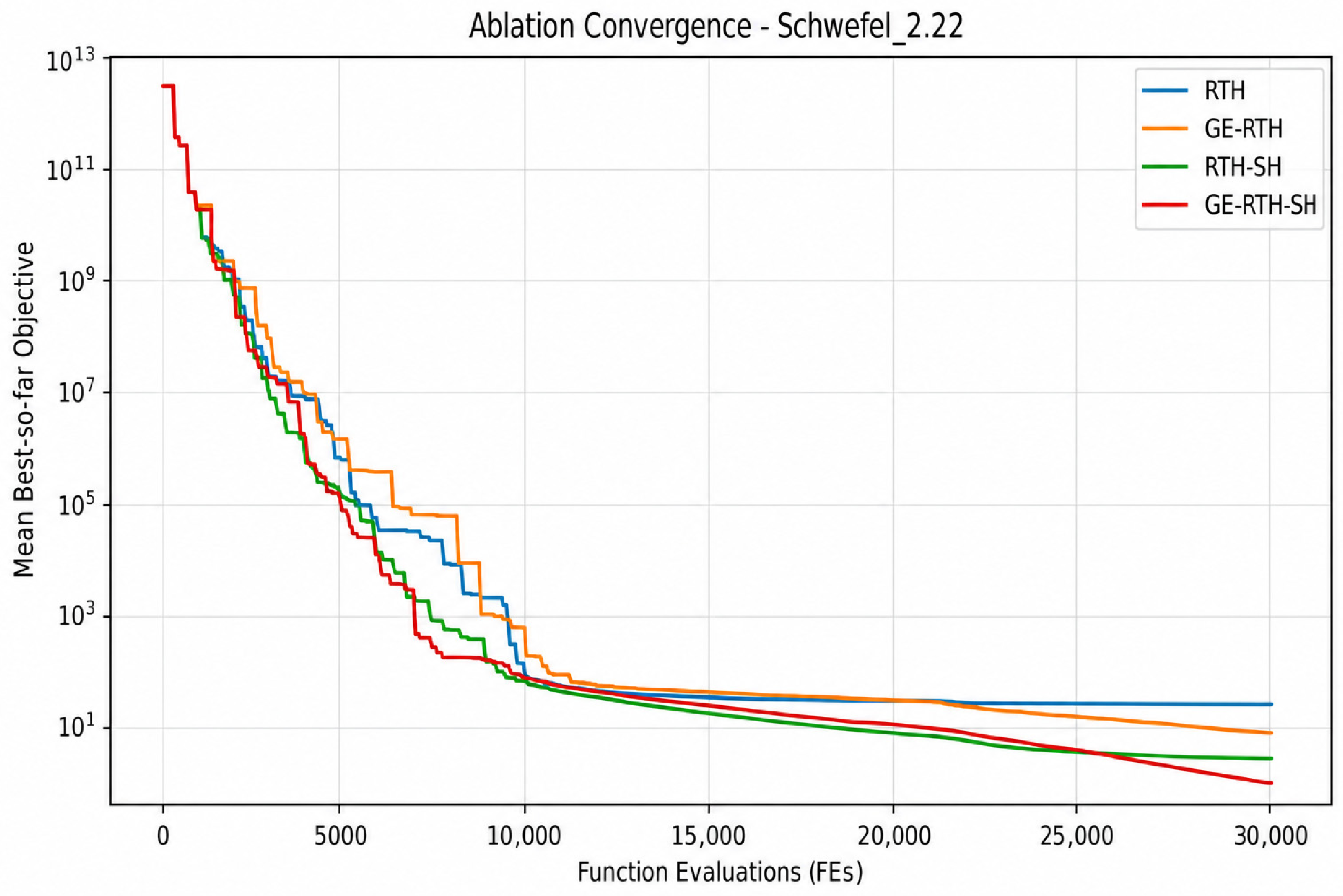
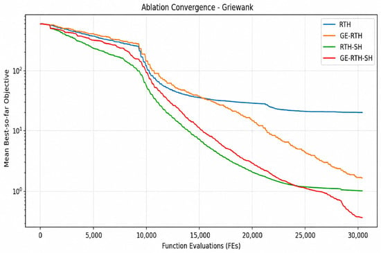
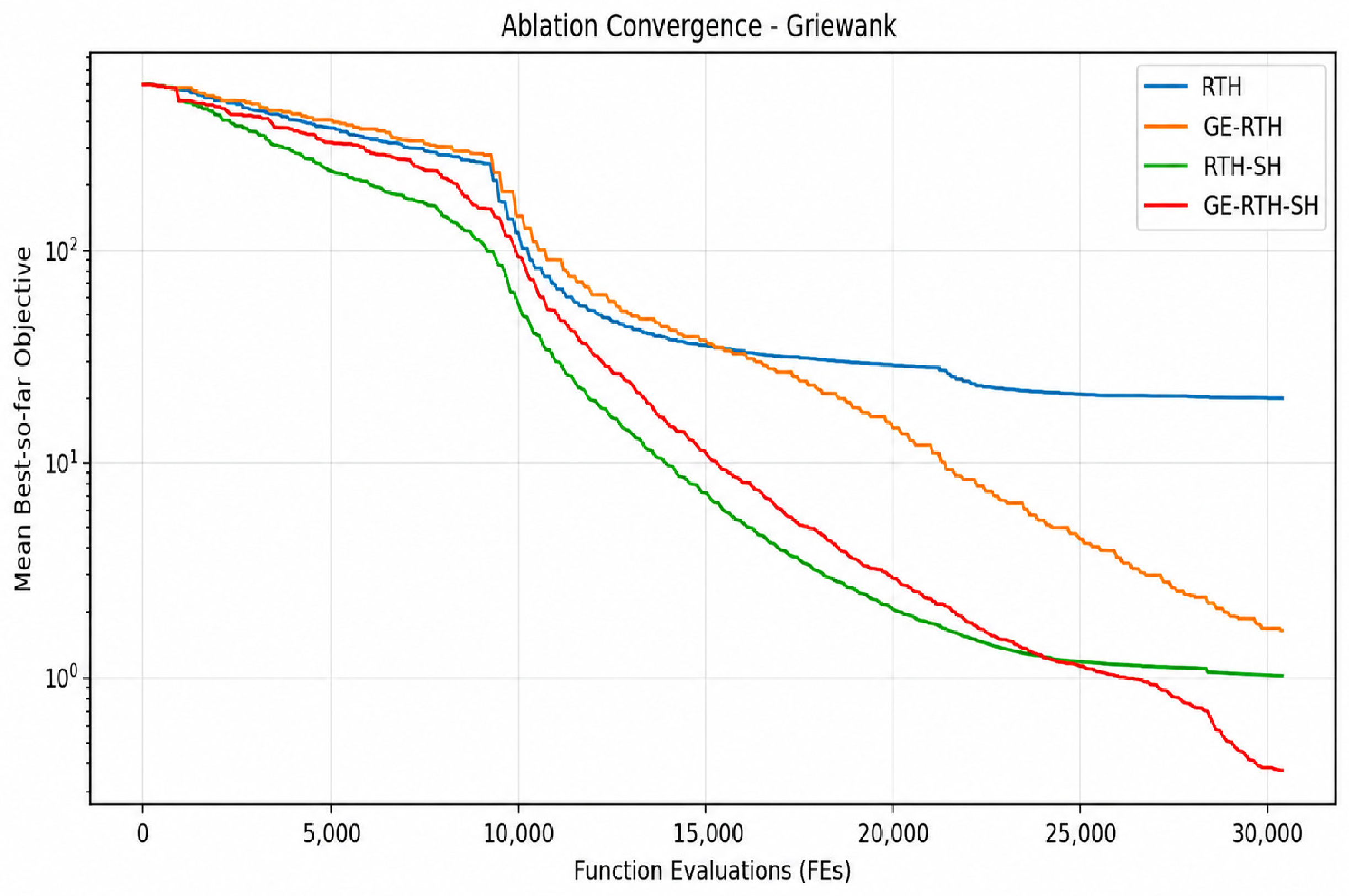
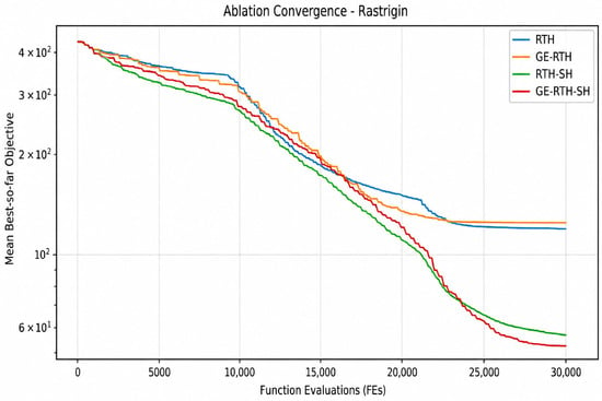
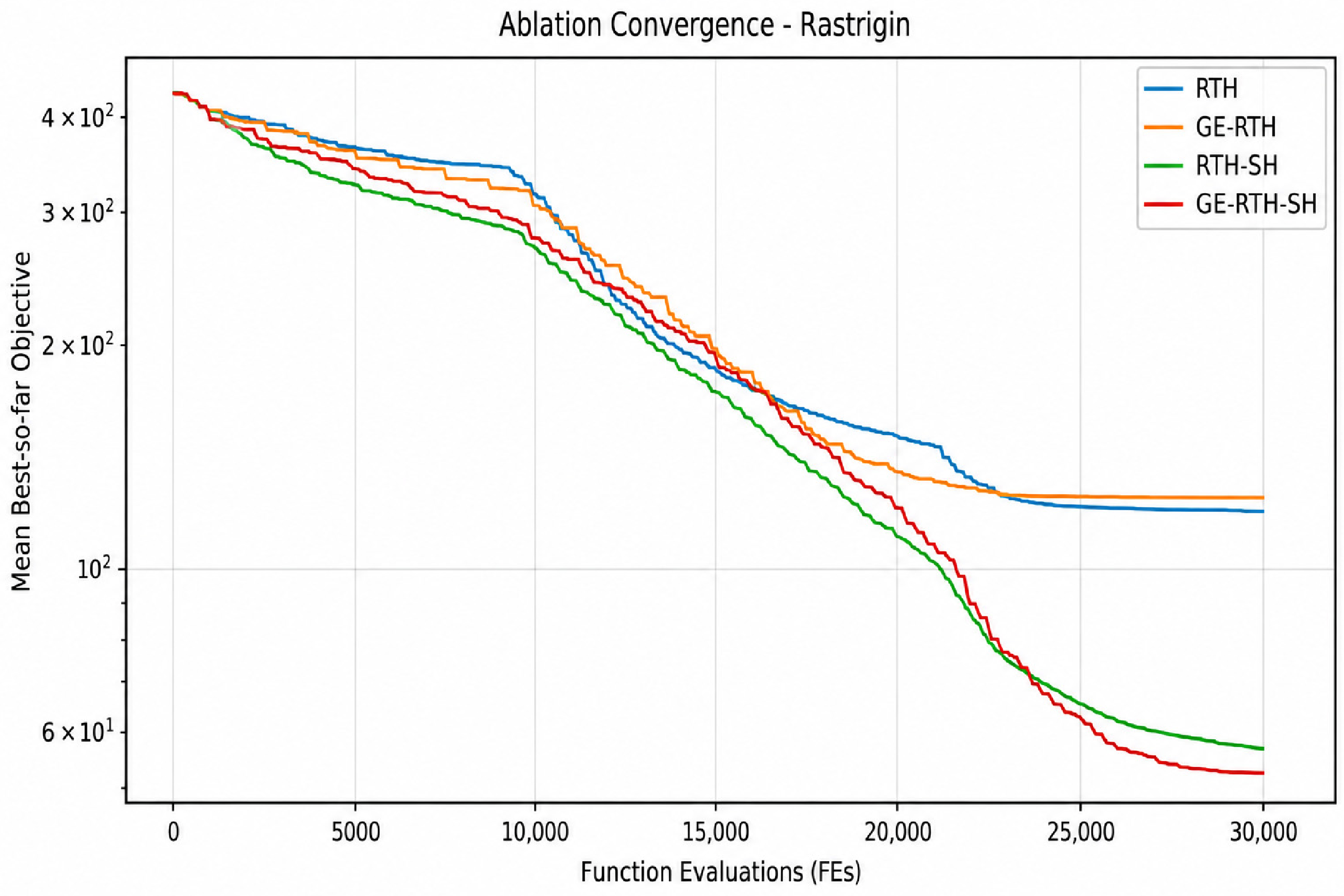
To quantify the contributions of the gradient-guided elite strategy (GE) and SHADE-lite mechanism (SH), four variants RTH, GE-RTH, RTH-SH, and GE-RTH-SH are compared. All variants use the same population size and a common maximum number of function evaluations, with MaxFEs = 30,000, thereby ensuring a consistent computational budget. Sphere, Rosenbrock, Schwefel 2.22, Rastrigin, and Griewank are used as test functions, and best, mean, Std, and MaxFEs are reported over 30 independent runs.

As shown in Figure 9, Figure 10, Figure 11, Figure 12 and Figure 13 and Table 3 and Table 4, the basic RTH has relatively limited accuracy on the five test functions, whereas adding GE or SH improves performance on most functions. In Table 4, “+”, “−”, and “≈” indicate that the former algorithm performs better than, worse than, and comparably to the latter algorithm, respectively. The SH module provides the most consistent enhancement. For Sphere, the mean objective value decreases from 1853.313775 for RTH to 14.388628 for RTH-SH, and further to 0.144243 for GE-RTH-SH, with a best value of 4.0 × 10⁻⁵. This indicates that SH substantially strengthens the search capability, while GE further refines high-quality solutions.

Figure 9. Sphere ablation test.

Figure 10. Rosenbrock ablation test.

Figure 11. Schwefel 2.22 ablation test.

Figure 12. Griewank ablation test.

Figure 13. Rastrigin ablation test.

Table 3. Results of the ablation experiments.

Function	Algorithm	Best	Mean	Std	MaxFEs	Iterations	CPU Time (s)
Griewank	GE-RTH	1.07	1.71	0.83	30,000	122	0.51
Griewank	GE-RTH-SH	0.11	0.40	0.19	30,000	95	0.74
Griewank	RTH	9.92	20.26	7.96	30,000	150	0.51
Griewank	RTH-SH	0.81	1.06	0.08	30,000	110	0.79
Rastrigin	GE-RTH	47.76	125.51	41.07	30,000	122	0.41
Rastrigin	GE-RTH-SH	26.14	53.10	16.19	30,000	95	0.66
Rastrigin	RTH	59.46	120.25	27.00	30,000	150	0.41
Rastrigin	RTH-SH	28.29	57.28	16.51	30,000	110	0.72
Rosenbrock	GE-RTH	631.77	12,675.60	12,236.20	30,000	122	0.46
Rosenbrock	GE-RTH-SH	36.18	316.84	465.25	30,000	94	0.71
Rosenbrock	RTH	167,027.24	778,402.83	457,586.52	30,000	150	0.45
Rosenbrock	RTH-SH	118.83	517.05	595.22	30,000	109	0.76
Schwefel 2.22	GE-RTH	1.04	7.17	4.61	30,000	122	0.39
Schwefel 2.22	GE-RTH-SH	0.16	0.84	0.68	30,000	94	0.63
Schwefel 2.22	RTH	15.32	22.76	4.28	30,000	150	0.38
Schwefel 2.22	RTH-SH	0.75	2.47	1.31	30,000	109	0.68
Sphere	GE-RTH	4.26	81.36	68.63	30,000	122	0.43
Sphere	GE-RTH-SH	4.00 × 10−5	0.14	0.40	30,000	95	0.56
Sphere	RTH	634.52	1853.31	746.25	30,000	150	0.64
Sphere	RTH-SH	1.19	14.39	31.87	30,000	110	0.63

Table 4. Pairwise comparison of the ablation results.

Comparison	Sphere	Rosenbrock	Schwefel 2.22	Rastrigin	Griewank	+/≈/−
GE-RTH vs. RTH	+	+	+	≈	+	4/1/0
RTH-SH vs. RTH	+	+	+	+	+	5/0/0
GE-RTH-SH vs. RTH-SH	+	+	+	≈	+	4/1/0
GE-RTH-SH vs. GE-RTH	+	+	+	+	+	5/0/0
GE-RTH-SH vs. RTH	+	+	+	+	+	5/0/0

A similar improvement is observed on Rosenbrock. The mean value decreases from 778,402.825557 for RTH to 12,675.602879 for GE-RTH and 517.052880 for RTH-SH, while GE-RTH-SH achieves a mean of 316.837692 and a best value of 36.177356. Relative to RTH, the mean objective value of GE-RTH-SH is reduced by approximately 99.96%; relative to RTH-SH, it is further improved by about 38.72%. These results indicate that GE directional refinement complements SH population-based search on the strongly coupled, narrow-valley Rosenbrock landscape.

The Schwefel 2.22 results show the same general trend. The mean values of RTH, GE-RTH, RTH-SH, and GE-RTH-SH are 22.757280, 7.164555, 2.465131, and 0.835691, respectively. Compared with RTH, the mean result of GE-RTH-SH improves by approximately 96.33%; compared with RTH-SH, it improves by a further 66.10%. Its standard deviation of 0.677618 is also lower than the 1.309137 obtained by RTH-SH, indicating improved accuracy and stability on this function.

For the multimodal Griewank function, the mean values are 20.258161 for RTH, 1.706348 for GE-RTH, 1.057265 for RTH-SH, and 0.397264 for GE-RTH-SH. Relative to RTH-SH, GE-RTH-SH improves the mean result by approximately 62.43%, showing that GE can further refine solutions even when SH already provides strong global exploration.

Rastrigin reveals a more complex interaction between the two modules. The mean value of RTH is 120.251445, whereas GE-RTH yields 125.512848, indicating that GE alone does not improve this case. By contrast, RTH-SH reduces the mean to 57.277163 and GE-RTH-SH further reduces it to 53.097232. Thus, GE is problem-dependent when used alone on highly multimodal landscapes, where gradient guidance may encourage concentration around local optima. When combined with the stronger global exploration supplied by SH, however, GE still provides additional local refinement, improving the mean by about 7.30% relative to RTH-SH.

Across the five benchmark functions, SH is the more consistently beneficial module: RTH-SH improves the mean result on all five functions relative to the basic RTH. GE primarily strengthens local exploitation and its standalone benefit is problem-dependent, although clear gains are observed on Sphere, Rosenbrock, Schwefel 2.22, and Griewank. The complete GE-RTH-SH achieves lower mean objective values than RTH-SH on all five functions, with particularly marked improvements on Sphere, Rosenbrock, Schwefel 2.22, and Griewank. These results further demonstrate the asymmetric yet complementary roles of the two mechanisms: SH mainly preserves global search capability and population diversity, whereas GE selectively strengthens local refinement. Their combination therefore provides a more balanced exploration–exploitation process than either mechanism alone.

3.4.2. Computational Cost Analysis

As shown in Table 5, the overall average number of iterations for RTH, GE-RTH, RTH-SH, and GE-RTH-SH are 150.00, 122.00, 109.60, and 94.60 times, respectively. Among them, the average number of iterations for GE-RTH-SH is approximately 36.96% lower than that of the original RTH, making it the lowest among the four algorithms. This indicates that for the original RTH, each iteration mainly involves the execution of the predetermined population position update and fitness evaluation; while after introducing GE or SH, a single iteration may also include additional local search or differential candidate solution evaluation. Therefore, under the same function evaluation budget, the algorithm with the auxiliary search mechanism may complete all function evaluations with fewer outer iteration rounds.

Table 5. Comparison of computational overhead under the same function-evaluation budget.

Algorithm	Mean Iterations	Mean CPU Time (s)	MaxFEs
RTH	150.00	0.4780	30,000
GE-RTH	122.00	0.4400	30,000
RTH-SH	109.60	0.7160	30,000
GE-RTH-SH	94.60	0.6600	30,000

From the perspective of actual CPU running time, the overall average running time of the original RTH is 0.4780 s, GE-RTH is 0.4400 s, RTH-SH is 0.7160 s, and GE-RTH-SH is 0.6600 s. Compared with the original RTH, the average CPU running time of GE-RTH-SH has increased, indicating that after introducing gradient estimation, adaptive differential search, and related parameter update processes, there is still additional computational overhead. On the other hand, compared with RTH-SH that only introduced SHADE-lite, the overall average CPU running time of GE-RTH-SH has decreased from 0.7160 s to 0.6600 s, a reduction of approximately 7.8%. This shows that under the conditions of this group of tests, the combined application of GE and SHADE-lite does not lead to a longer overall average running time than RTH-SH, and to some extent, it reduces the running time of RTH-SH.

Further analysis based on the ablation experiment results in Table 3 reveals that although the average CPU running time of GE-RTH-SH is not the shortest among the four algorithms, under the condition of MaxFEs = 30,000, it achieves the lowest average objective function value on all five test functions. For example, in the Rosenbrock function, the average objective function value of GE-RTH-SH is reduced from the original RTH’s 778,402.825557 to 316.837692; in the Rastrigin function, it is reduced from 120.251445 to 53.097232. These results indicate that although the auxiliary search strategy introduces some computational overhead, it can improve the final solution accuracy within the given function evaluation budget.

From the perspective of algorithm design, this paper does not increase the number of iterations continuously to improve optimization performance, but rather retains the original three-stage mechanism of RTH (high-altitude circling, low-altitude circling, and dive hunting), and coordinates the search tasks of different stages through gradient-guided elite search and SHADE-lite adaptive differential search. Among them, gradient search focuses on some dominant individuals and limits their calling frequency by setting a search interval; SHADE-lite is selectively enabled based on the search progress and stagnation status to avoid executing the auxiliary differential search unconditionally throughout all iterations. At the same time, the algorithm adopts a unified maximum objective function evaluation times limit to calculate the budget, allowing different search operations to complete within the given budget.

The statistical results of optimization accuracy, number of iterations, and CPU running time show that GE-RTH-SH demonstrates better solution accuracy in this group of tests, but still has some additional computational time overhead. Therefore, the main advantage of the proposed algorithm is not to achieve the shortest running time under all test conditions, but to obtain higher-quality optimization results with better balance between solution accuracy and computational cost through the collaborative use of search strategies with different functions, under a fixed function evaluation budget.

Overall, the ablation experiments on five 30-dimensional standard test functions verified the complementary effect of GE and SH under the current test conditions. SHADE-lite can relatively stably improve the optimization results of the original RTH, while the gradient-guided elite search mainly further strengthens the local development of the advantageous areas and shortens the number of iterations and running time. After combining the two mechanisms, GE-RTH-SH achieved better average solution results on all five functions, indicating the effectiveness of this asymmetric complementary search framework. At the same time, the computational cost analysis further clarified the time cost brought by the auxiliary search operation and its corresponding accuracy gain, providing an experimental basis for the subsequent application of GE-RTH-SH to the economic dispatch problem of microgrids with multi-period coupling and operation constraints.

4. Case Study

4.1. Basic Parameter Settings

To evaluate GE-RTH-SH for coordinated scheduling in a microgrid with a high penetration of renewable energy, a grid-connected system comprising WT, PV, MT, FC, ESS, and the utility grid is constructed. WT and PV are the main renewable sources; MT and FC are controllable distributed generators; the ESS provides energy shifting and power regulation; and the utility grid enables electricity import and export. The study focuses on 24 h day-ahead operation rather than capacity planning. Therefore, all installed capacities are treated as known parameters and one-time investment costs are excluded. The operating objective includes equipment O&M costs, MT and FC fuel costs, ESS operating costs, and the net cost of electricity transactions with the utility grid. To test scheduling under high renewable output, the WT and PV capacities are expanded for the case-study scenario, while technical inputs for MT, FC, and ESS are drawn from [9], where available, and the representative 4 h ESS capacity is a scenario assumption informed by [20]. Based on the 24 h day-ahead scheduling cycle and a 1 h time interval, the entire day is divided into 24 scheduling periods. Among them, the purchase and sale electricity prices for periods 1 to 9 are 0.216 CNY/kWh and 0.155 CNY/kWh, respectively; periods 10 to 13 are 0.793 CNY/kWh and 0.485 CNY/kWh, respectively; periods 14 to 18 are 0.505 CNY/kWh and 0.315 CNY/kWh, respectively; periods 19 to 24 are 0.793 CNY/kWh and 0.485 CNY/kWh respectively. Thus, this provides a unified electricity price input condition for the 24 h economic scheduling optimization. Accordingly, the parameters in Table 6 define an algorithmic test scenario and do not represent measured data from a specific real-world microgrid.

Table 6. Main operating parameters of the microgrid.

Unit	Rated Power (kW)	O&M Cost (CNY/kWh)	Efficiency	Fuel Price (CNY/kg)	Lower Heating Value (kJ/g)	Ramp Rate/Notes
WT	2200	0.031	—	—	—	—
PV	1320	0.019	—	—	—	—
MT	120	0.012	0.40	5.14	51.257	Minimum stable output: 24 kW; ramp rate: ±17 kW/h
FC	120	0.017	0.51	2.43	22.687	Minimum stable output: 18 kW; ramp rate: ±12 kW/h
ESS	100	0.005	Charging efficiency: 0.82; discharging efficiency: 0.93	—	—	Energy capacity: 400 kWh; SOC range: 0.20–0.80; initial/terminal SOC = 0.50

This example uses the constructed 24 h aggregated load curve instead of the measured data at the residential user level. The model does not set the number of residential households, nor does it describe the detailed feeder topology. The loads from hour 1 to hour 24 are successively 650, 600, 580, 560, 550, 580, 700, 850, 950, 980, 1050, 1100, 1150, 1200, 1150, 1100, 1050, 1100, 1150, 1050, 950, 850, 750 and 700 kW. The peak load for the entire day is 1200 kW.

4.2. Computational Environment and Experimental Parameter Settings

To ensure the reproducibility of the proposed GE-RTH-SH algorithm and its experimental results in the economic dispatch of grid-connected microgrids, this paper provides a unified description of the computational environment, algorithm parameters, microgrid system configuration, input data, and experimental operating conditions. All optimization algorithms are executed under the specified computational budget and constraints to enhance the comparability of the experimental results of different algorithms.

This paper implements the GE-RTH-SH algorithm and the microgrid economic dispatch model using Python in the PyCharm 2024.1 integrated development environment. NumPy 2.3.2 is mainly used for numerical calculations, and Matplotlib 3.10.7 is used for visualizing the experimental results. The microgrid economic dispatch adopts a 24 h day-ahead scheduling cycle with a time resolution of 1 h, and is divided into 24 scheduling periods. The optimization decision vector includes the output power of the microturbine (MT), the output power of the fuel cell (FC), the charging and discharging power of the energy storage system (ESS), and the exchange power with the main grid. Each type of variable corresponds to 24 periods. To control the computational budget of different optimization algorithms, the maximum number of function evaluations of the objective function (MaxFEs) is used as the termination condition. The population size of the GE-RTH-SH algorithm is set to 50, and the maximum number of function evaluations of the objective function is set to 30,000. The additional function evaluations generated by gradient-guided local search are also included in the computational budget.

The GE-RTH-SH algorithm is based on the original RTH three-stage search mechanism and introduces gradient-guided elite local search (GE) and SHADE-lite adaptive differential search (SH) to enhance local exploitation capability and global search diversity. The main algorithm parameters are shown in Table 7.

Table 7. Main parameter settings of the GE-RTH-SH algorithm.

Parameter	Symbol or Code Variable	Value
Population size	population_size	50
Maximum number of function evaluations	max_fes	30,000
Gradient search module	use_gradient	True
SHADE-lite module	use_shade	True
Elite ratio	elite_ratio	0.05
Gradient search interval	gradient_interval	5
Central-difference step size	gradient_h	1 × 10−6
Base gradient search step size	gradient_step	0.003
Initial scaling-factor memory	shade_Fm0	0.50
Initial crossover-probability memory	shade_CRm0	0.70
p-best ratio	shade_p	0.20
External archive capacity factor	shade_archive_factor	2.0
SHADE-lite activation progress ratio	shade_start_ratio	0.25
Consecutive stagnation trigger threshold	shade_stagnation_trigger	4

A feasibility evaluation independent of the target penalty value was conducted for the scheduling scheme of GE-RTH-SH. The maximum power balance error, terminal SOC error, maximum climbing limit of each device, upper and lower limits of grid power, as well as whether simultaneous charging-discharging or simultaneous purchase-sale of electricity occurred were listed. The program adopted sequential SOC repair, output truncation, and grid balance reconstruction. A part of the upper limit of the grid import was guaranteed through a secondary penalty. Table 8 reports the independent verification results of the key constraints for the selected representative scheduling scheme, with a tolerance of 10⁻⁵.

Table 8. Independent constraint verification for the selected GE-RTH-SH schedule.

Constraint Check	Verified Value	Tolerance/Interpretation
Power balance, max |residual|	0.00 kW	≤1 × 10−5 kW
SOC, minimum/maximum	0.200000/0.800000	Bounds 0.20–0.80
Terminal SOC absolute error	0.00	≤1 × 10−5
ESS simultaneous charge/discharge	0	0 h
Grid simultaneous import/export	0	0 h
Grid maximum import violation	0.00 kW	≤1 × 10−5 kW
MT/FC maximum ramp violation	0.00 kW/h	≤1 × 10−5 kW/h

4.3. Stability Analysis of Simulation Results

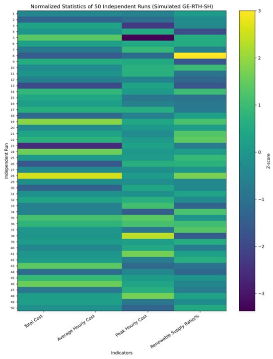
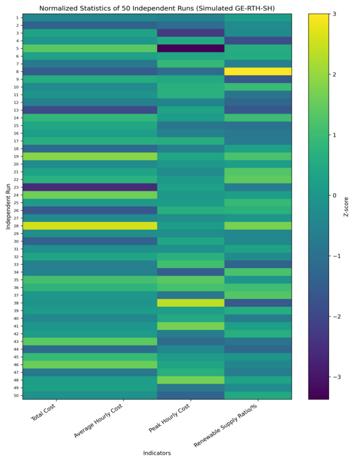
To evaluate repeatability for the stochastic optimization method, 50 independent runs are performed. The mean, standard deviation (Std), maximum, minimum, and coefficient of variation (CV) are calculated for the total operating cost and related indicators.

$$\mathit{CV}\%={\displaystyle \frac{\Delta }{\mu }}\times 100\%$$

(31)

Here, Std denotes the standard deviation and mean denotes the arithmetic mean. A smaller CV indicates lower dispersion among independent runs; however, the CV alone does not establish global optimality.

Table 9 and Figure 14 summarize the 50 independent runs of GE-RTH-SH. The CV of total operating cost is 0.1890%, indicating consistent economic-dispatch results under different random initializations. The renewable energy supply ratio has a CV of 0.3356%, showing similarly good repeatability. The peak hourly cost exhibits a larger CV of 2.0588%, indicating greater variability in local peak-cost periods. Overall, the results demonstrate good repeatability across independent runs.

Table 9. Stability statistics over 50 independent runs.

Indicator	Runs	Mean	Std	Maximum	Minimum	CV (%)
Total Cost (CNY)	50	5295.06	10.01	5320.93	5269.11	0.19
Average Hourly Cost (CNY)	50	220.63	0.42	221.71	219.55	0.19
Peak Hourly Cost (CNY)	50	575.69	11.85	603.84	535.73	2.06
Renewable Energy Supply Ratio (%)	50	62.55	0.21	63.18	62.16	0.34

Figure 14. Heatmap of normalized statistics from 50 independent runs.

4.4. Economic Dispatch Results and Constraint Verification

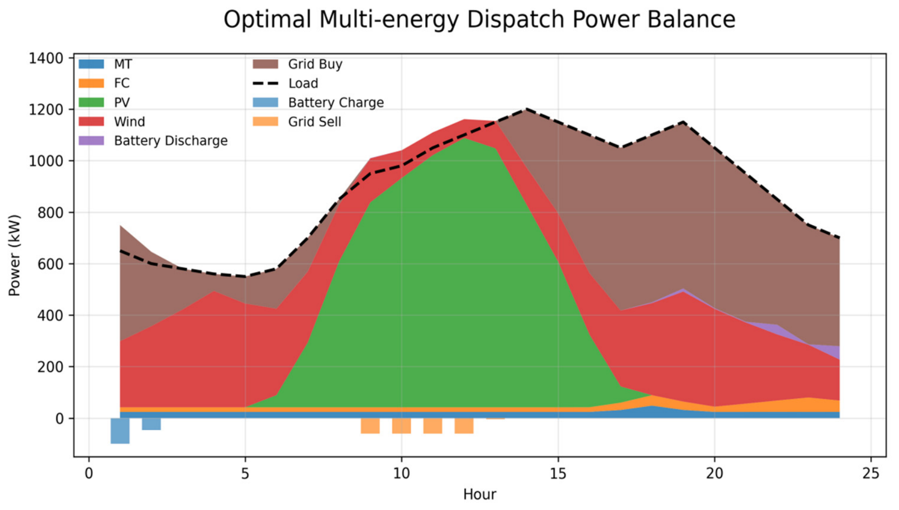
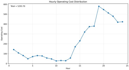
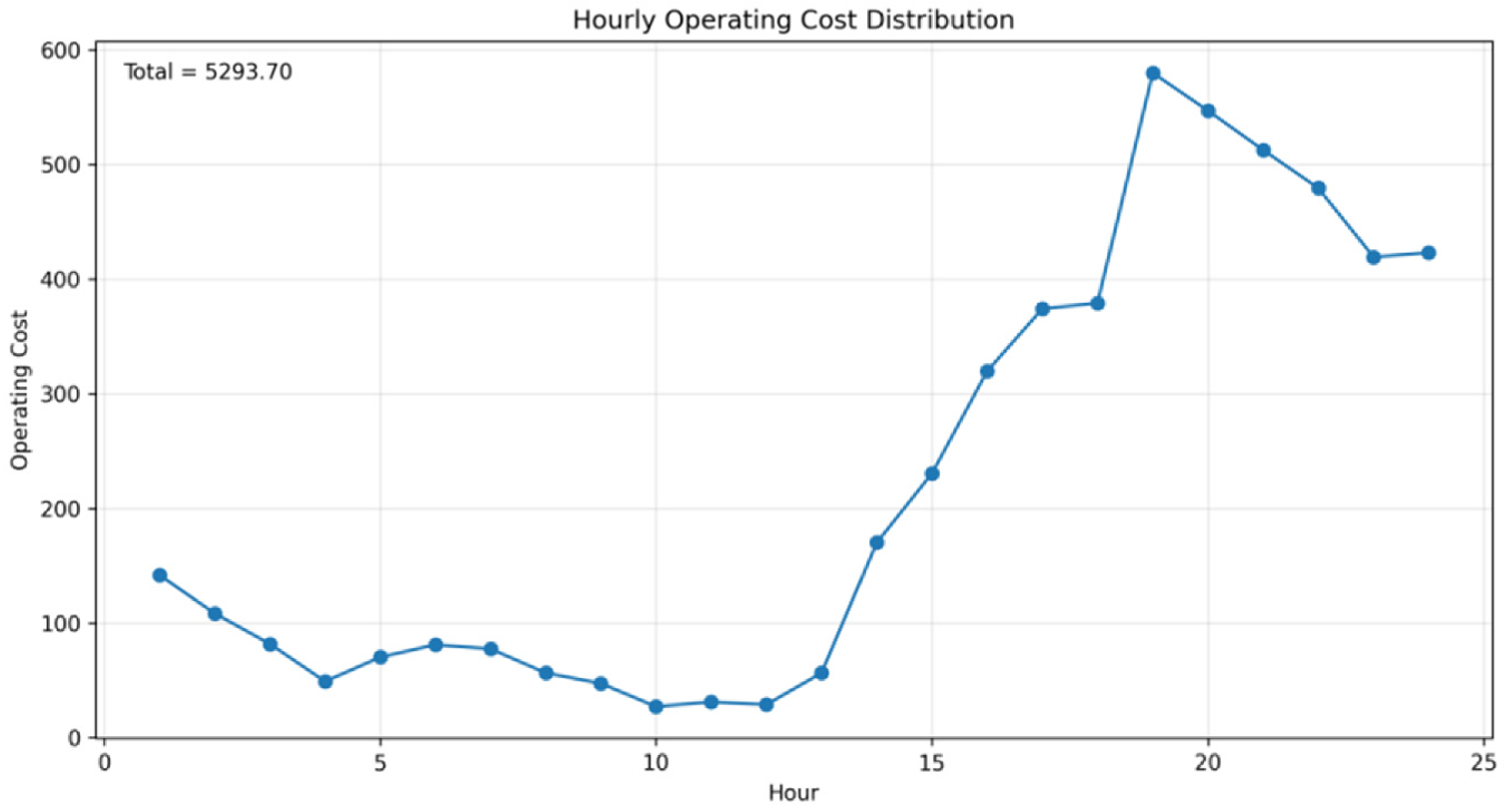
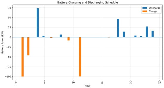
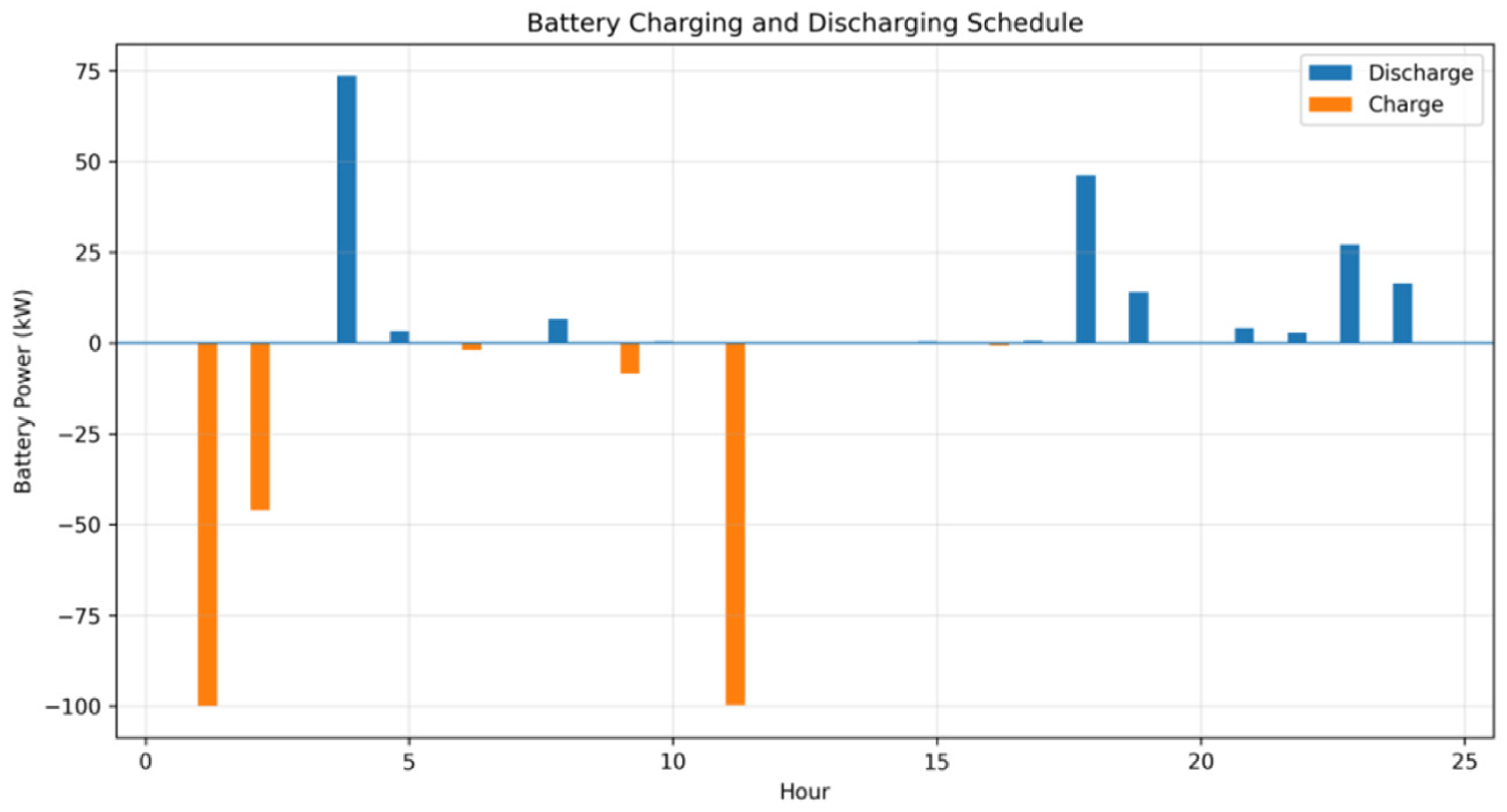
To distinguish between a single scheduling example and the statistical results of multiple independent runs, Figure 15, Figure 16, Figure 17, Figure 18 and Figure 19 present the 24 h scheduling plan obtained from the same run. The total 24 h operating cost corresponding to Figure 17 is CNY 5293.70. The CNY 5295.06 reported in the stability statistics table is the average total 24 h cost of 50 independent runs. The statistical bases are different and are used to show the specific scheduling process and the stability of the evaluation results, respectively.

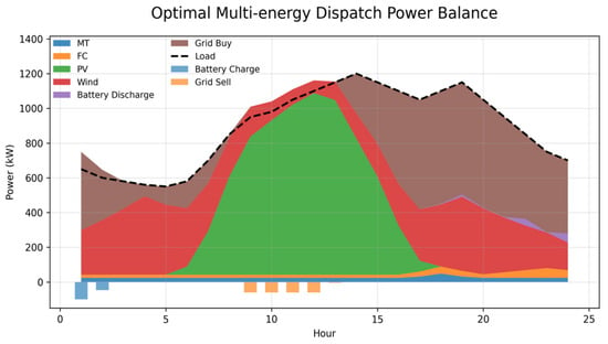
Figure 15. GE-RTH-SH power dispatch profile.

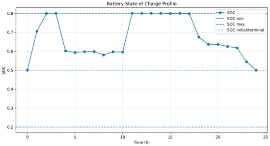
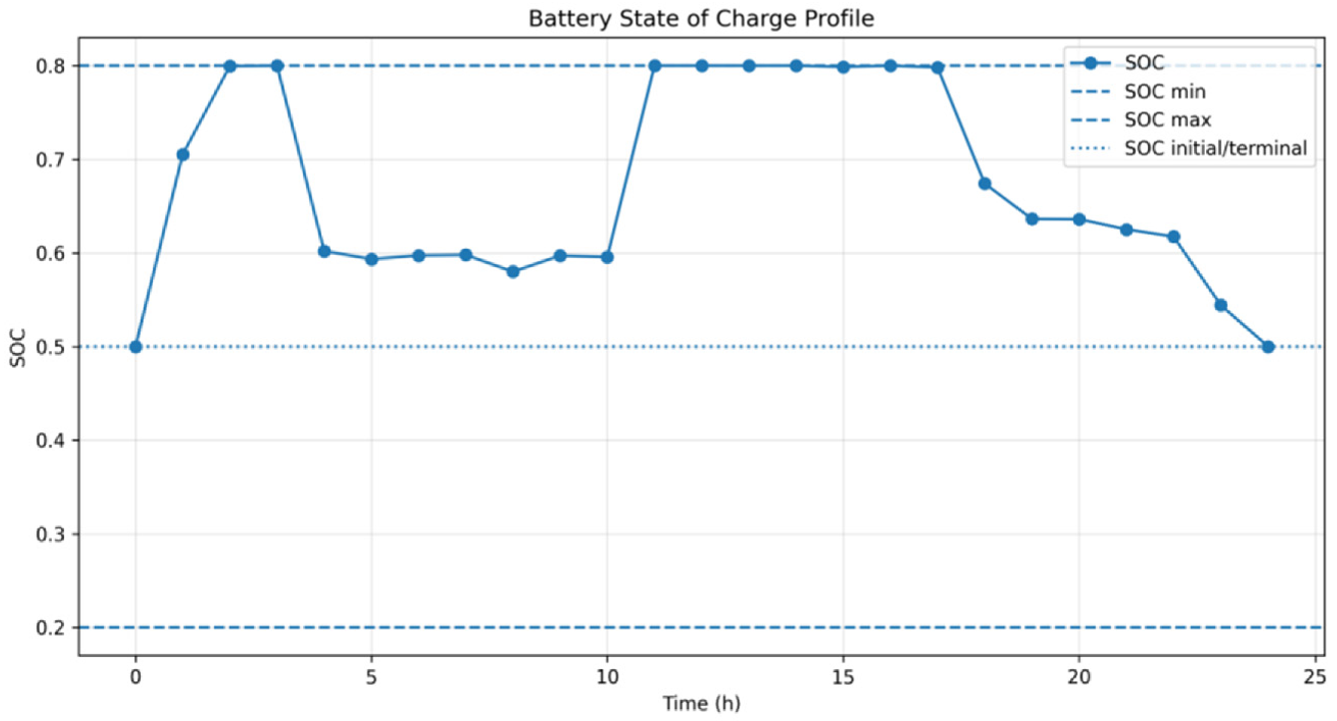
Figure 16. Twenty-four-hour ESS state-of-charge profile.

Figure 17. Hourly operating cost under GE-RTH-SH.

Figure 18. ESS charging and discharging power profile.

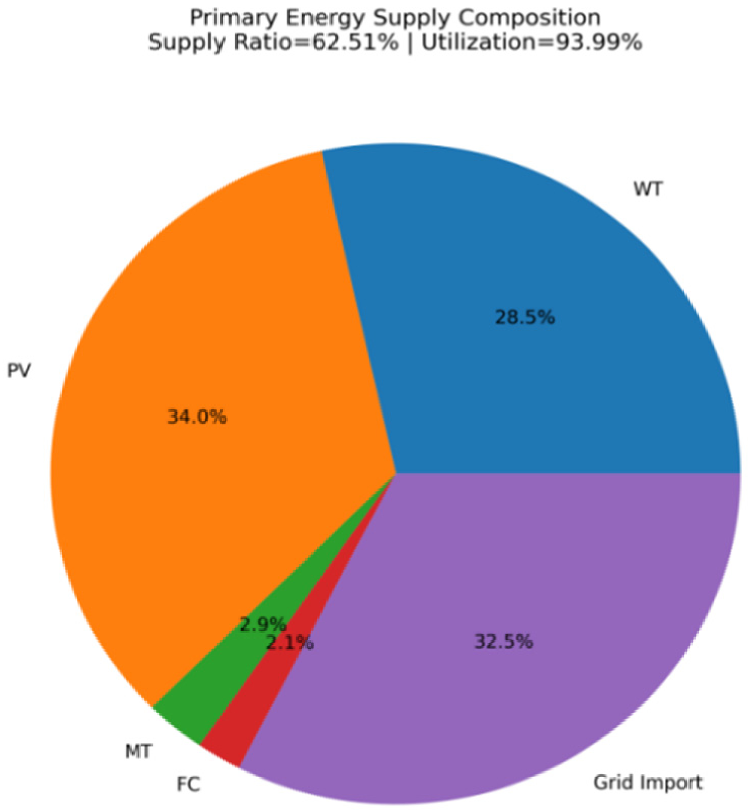
Figure 19. Primary energy supply composition.

Figure 15 shows the 24 h dispatch of the distributed energy sources, ESS, and grid exchange. The dashed curve represents system load. Positive power comprises MT, FC, PV, wind generation, ESS discharge, and grid imports, whereas negative power represents ESS charging and grid exports. When charging or export occurs, the upper boundary of the positive-power stack can exceed the load curve because the excess is absorbed by the ESS or exported through the tie line; this does not indicate a power imbalance. The representation is consistent with the balance relation ‘generation + ESS discharge + grid import = load + ESS charge + grid export’. From late night to early morning, PV output is negligible and demand is mainly supplied by wind generation and grid imports, while MT and FC maintain low but continuous outputs. Around hour 1, the ESS charges using surplus or low-cost electricity, creating flexibility for later high-load periods. As solar irradiance increases, PV output rises rapidly from approximately hour 6 and becomes the dominant supply around midday. Grid imports decrease accordingly. During approximately hours 9–12, high combined wind and PV output leads to some grid export. In the afternoon, PV output declines while load remains relatively high, so grid imports increase to compensate for the supply gap. Around hours 18–20, when PV output is nearly zero and load remains high, wind generation, grid imports, small contributions from MT and FC, and ESS discharge jointly maintain the power balance.

From the 24 h scheduling results, it can be seen that the wind power output maintains a relatively continuous change throughout the day, while the photovoltaic power generation has obvious diurnal characteristics. The two undertake different power supply tasks at different time periods. When the photovoltaic output increases during the day, the system’s demand for purchasing electricity from the main grid decreases. During some periods with higher output from renewable energy sources, the excess electricity can also be sent to the main grid. As the photovoltaic output decreases in the afternoon, externally purchased electricity gradually assumes more load compensation tasks. The micro gas turbine and fuel cell provide relatively stable auxiliary output during the scheduling period, while the energy storage system adjusts charging and discharging based on the system’s supply and demand. Thus, the microgrid completes the power supply arrangement by coordinating local power generation, energy storage operation, and power exchange with the main grid. The illustrated scheduling results reflect the coordinated relationship of various energy sources on the time scale.

Figure 16 shows the 24 h ESS state-of-charge profile. The initial SOC is 0.50 and remains within the allowable range of 0.20–0.80 throughout the scheduling horizon. During the initial period, SOC rises from 0.50 to 0.80, indicating charging, and then falls to approximately 0.60 as the ESS discharges. SOC varies slightly around 0.60 during the intermediate period and reaches 0.80 again at approximately hour 11. It then remains near the upper limit for several hours before gradually decreasing after hour 17 and returning to 0.50 at the end of the horizon. The resulting trajectory verifies compliance with the SOC bounds and the terminal-state constraint.

Figure 17 presents the hourly operating cost over the 24 h horizon, with a total operating cost of CNY 5293.70. Costs remain relatively low from early morning to noon and reach their daily minimum around hours 10–12, when wind and PV supply a large share of demand and reduce conventional generation and grid-purchase costs. After hour 14, PV output declines while load remains high, increasing reliance on grid imports and other dispatchable sources; the hourly cost consequently rises and reaches its daily peak around hour 19. Costs then decrease as the load falls. Thus, the hourly operating cost follows the combined temporal patterns of load, renewable output, and grid-purchase requirements.

Figure 18 shows the ESS charging and discharging power over 24 h, which is consistent with the SOC trajectory. Negative power denotes charging and positive power denotes discharging. During hours 1–2, the ESS charges at a relatively high rate, increasing SOC from 0.50 to 0.80. Around hour 4, a marked discharge reduces SOC to approximately 0.60. ESS power remains relatively small during the middle period, except for several short charging/discharging events. Around hour 11, another charging event raises SOC to 0.80. After hour 18, the ESS gradually switches to discharge and releases stored energy over several consecutive intervals, returning to the initial SOC of 0.50 by the end of the scheduling horizon. The profile confirms cross-period energy shifting while satisfying the SOC boundary and terminal-state constraints.

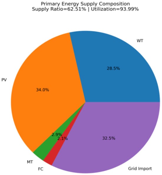
Figure 19 shows the primary energy supply composition. PV, WT, and grid imports account for 34.0%, 28.5%, and 32.5%, respectively, while MT and FC contribute smaller shares of 2.9% and 2.1%. The renewable energy supply ratio, defined as the combined contribution of wind and PV, is therefore 62.51%. The result indicates that the microgrid relies primarily on wind and solar resources, with the utility grid providing an important supplementary balancing function.

To comprehensively evaluate the solution performance of the GE-RTH-SH algorithm in the economic dispatch problem of microgrids, this paper selects two representative optimization methods for comparison: one is meta-heuristic optimization algorithms, including Particle Swarm Optimization (PSO), Whale Optimization Algorithm (WOA), Ant Colony Optimization Algorithm (DBO), and the original Red-tailed Hawk Optimization algorithm (RTH); the other is mathematical programming methods, including Sequential Least Squares Programming (SLSQP) and Limited Memory BFGS Bound-Constrained Optimization Method (L-BFGS-B). Under the same function evaluation budget (MaxFEs = 30,000), each algorithm is set to conduct 50 independent solution attempts. The related costs and performance results are listed in Table 10. The cost statistics of the mathematical programming methods are based on the results of strict feasibility verification.

Table 10. Comparison of microgrid economic-dispatch performance.

Algorithm	Starts	Best Cost (CNY)	Mean Cost (CNY)	Std	MaxFEs	Renewable Energy Supply Ratio
GE-RTH-SH	50	5269.11	5295.06	10.01	30,000	0.6255
DBO	50	5281.66	5315.18	13.09	30,000	0.6256
WOA	50	5302.55	5353.98	29.80	30,000	0.6099
PSO	50	5335.31	5386.29	28.62	30,000	0.6046
RTH	50	5331.42	5354.69	19.92	30,000	0.6164
SLSQP	50	5297.68	5409.31	75.10	30,000	0.6266
L-BFGS-B	50	5307.75	5564.82	178.56	30,000	0.6188

In the comparison of meta-heuristic algorithms, GE-RTH-SH achieved the lowest optimal operation cost and average operation cost, which were CNY 5269.11 and CNY 5295.06, respectively, and its standard deviation was only 10.01, indicating that this algorithm has better optimization accuracy and repeatability stability. Compared with the DBO algorithm, which has the second-best average operation cost, the average operation cost of GE-RTH-SH was reduced by CNY 20.12, a decrease of approximately 0.38%, and the standard deviation was reduced by approximately 23.53%; compared with the original RTH, its average operation cost was reduced by approximately 1.11%. At the same time, GE-RTH-SH also outperformed the PSO and WOA in terms of average operation cost and standard deviation, indicating that the introduction of gradient-guided elite search and SHADE-lite adaptive differential search can improve the optimization performance and repeatability stability of the original algorithm to a certain extent.

In the comparison with mathematical programming methods, the average operation cost and standard deviation of GE-RTH-SH were lower than SLSQP and L-BFGS-B, indicating that in the nonlinear, multi-variable coupled microgrid economic dispatch problem studied, GE-RTH-SH can obtain a dispatch scheme with lower cost and smaller operation result fluctuation under the given computational budget. This shows that the algorithm not only performs well in the comparison among meta-heuristic optimization algorithms but also has certain economic and stability advantages compared to the selected mathematical programming methods.

In terms of renewable energy utilization, the average renewable energy supply ratio of GE-RTH-SH was 62.55%, which was basically the same as that of the DBO algorithm (62.56%), slightly lower than that of the SLSQP algorithm (62.66%), but higher than the other comparison algorithms. Overall, GE-RTH-SH performed well in the economic dispatch comparison with meta-heuristic optimization algorithms and mathematical programming methods, achieving lower operation costs and better repeatability stability while maintaining a high renewable energy supply ratio. This further verifies the effectiveness of the proposed asymmetric complementary search framework in this microgrid economic dispatch scenario.

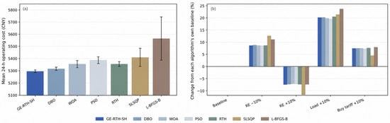
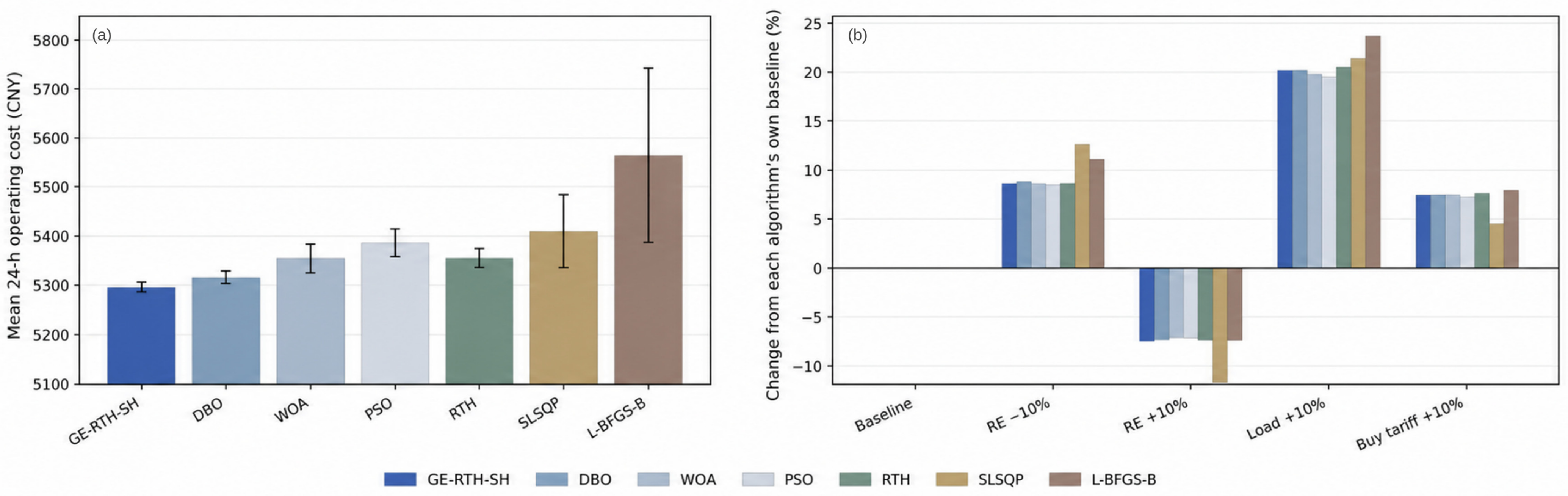
To evaluate the sensitivity of the 24 h operating conditions constructed under varying input conditions, this paper sets up four disturbance scenarios, namely a 10% reduction or increase in the available output of wind and solar power, a 10% increase in load demand, and a 10% increase in the purchase price of electricity. Table 11 presents the costs and statistics of renewable energy supply of GE-RTH-SH under the above conditions for 50 independent operations. Figure 20a summarizes the seven benchmark comparison results reported in Table 10, and Figure 20b shows the relative average cost responses of the seven algorithms implemented in the sensitivity experiments of each condition, run 10 times. The variation amplitudes in Figure 20b are normalized by the respective algorithm’s own benchmark mean to facilitate the comparison of the direction and magnitude of cost responses under different scenarios. The data in both figures come from different experimental batches, and this paper provides explanations accordingly.

Table 11. GE-RTH-SH sensitivity analysis based on 50 runs per changed operating condition.

Scenario	Mean Cost (CNY)	Std (CNY)	Mean RE Supply (%)
RE −10%	5753.28	15.76	57.99
RE +10%	4902.77	12.89	66.49
Load +10%	6355.39	19.04	58.37
Buy tariff +10%	5678.70	19.05	62.59

Figure 20. (a) Benchmark average running costs and standard deviations of the seven algorithms. (b) Relative average cost changes in the seven algorithms under four types of input perturbations.

In the original 50 GE-RTH-SH sensitivity experiments listed in Table 11, with the reported benchmark average cost of CNY 5295.06 as the reference, when the available wind and solar power decreased by 10%, the average cost increased to CNY 5753.28, while when the available wind and solar power increased by 10%, it decreased to CNY 4902.77; when the load demand and purchase electricity price increased by 10%, respectively, the average cost increased to CNY 6355.39 and CNY 5678.70. In the other batch of seven algorithm experiments shown in Figure 20b, the relative changes in GE-RTH-SH under corresponding disturbances were approximately +8.59%, −7.43%, +20.18% and +7.40%. The cost response directions of the seven algorithms were generally consistent, and the relative change amplitude of GE-RTH-SH was close to that of other meta-heuristic methods. These comparisons were mainly used to illustrate the cost sensitivity, and did not assume that the algorithm rankings of different experimental batches would always remain unchanged, or that each algorithm would generate the same physical scheduling scheme. Overall, the cost response pattern of GE-RTH-SH was clear; the relative change was similar to that of other meta-heuristic methods, and demonstrated good adaptability to test conditions and certain economic performance stability when facing moderate external input disturbances.

5. Conclusions and Outlook

This paper addresses the day-ahead economic dispatch problem of grid-connected microgrids, establishing a multi-energy coordinated operation model considering wind power, photovoltaic power, micro gas turbines, fuel cells, and energy storage systems. It proposes an improved Red-Tailed Hawk Optimization algorithm, GE-RTH-SH, which integrates gradient-guided elite search (GE) and SHADE-lite adaptive differential search (SH). Through standard test functions, ablation experiments, and microgrid economic dispatch examples, the effectiveness of the proposed method is verified. The main conclusions are as follows:

GE-RTH-SH retains the search structure of the original RTH, while introducing two complementary mechanisms: local refinement of elite solutions and adaptive differential exploration. On the selected standard test functions, SHADE-lite has a more sustained positive effect on improving the optimization results, while gradient-guided elite search provides additional ways for local exploration. The combination of these two strategies enables the proposed framework to exhibit good optimization capabilities on the tested benchmark problems.

GE-RTH-SH achieved good economic dispatch results in the constructed 24 h microgrid example. The average cost of 50 independent runs was CNY 5295.06, with the optimal cost being CNY 5269.11, and the standard deviation being 10.01. Compared with DBO and the original RTH, its reported average cost decreased by approximately 0.38% and 1.11%, respectively. It also demonstrated better economic performance compared to the selected PSO and WOA benchmark algorithms. The average renewable energy supply ratio reached 62.55%, demonstrating the coordinated effect of distributed generation, energy storage, and grid exchange power under the model’s operating constraints.

The operation condition experiments revealed the influence patterns of renewable energy available output, load, and purchase electricity prices on costs. The sensitivity results of the original GE-RTH-SH indicated that an increase in renewable energy available output could reduce costs, while a decrease in output, an increase in load, and a rise in purchase electricity prices would increase costs. The supplementary seven algorithm implementation comparison further showed that all algorithms have generally similar response directions, and the cost change amplitude of GE-RTH-SH is similar to other meta-heuristic methods. These phenomena support the adaptability of the proposed method to test operating conditions and indicate its economic performance stability under moderate external input disturbances.

In summary, the GE-RTH-SH hybrid search framework demonstrates good application potential in the coordinated economic operation of grid-connected microgrids. This method combines effective optimization performance on standard test functions, good economic dispatch results under benchmark conditions, and interpretable condition responses. In the future, the uncertainty of wind and solar power output and load prediction can be further considered, and the framework can be extended to rolling time domains and real-time scheduling to adapt to more complex microgrid operation scenarios.

References

- Han, X.; Li, T.; Zhang, D.; Zhou, X. New issues and key technologies of new power system planning under double carbon goals. High Volt. Eng. 2021, 47, 3036–3046. [Google Scholar] [CrossRef]
- Zhao, Z.; Zhang, M.; He, M.; Gao, Y.; Li, J.; Han, S.; Liu, Z.; Lei, L.; Díaz, J.I.P.; Cavazzini, G.; et al. Beyond fixed-speed pumped storage: A comprehensive evaluation of different flexible pumped storage technologies in energy systems. J. Clean. Prod. 2024, 434, 139994. [Google Scholar] [CrossRef] [Scilit]
- Lasseter, R.H. MicroGrids. In Proceedings of the 2002 IEEE Power Engineering Society Winter Meeting, New York, NY, USA, 27–31 January 2002; Volume 1, pp. 305–308. [Google Scholar] [CrossRef] [Scilit]
- Onsomu, O.N.; Terciyanlı, E.; Yeşilata, B. Comprehensive review of energy management strategies: Considering battery energy storage system and renewable energy sources. Eng. Rep. 2024, 6, e12995. [Google Scholar] [CrossRef] [Scilit]
- Jane, R.; Parker, G.; Vaucher, G.; Berman, M. Characterizing meteorological forecast impact on microgrid optimization performance and design. Energies 2020, 13, 577. [Google Scholar] [CrossRef] [Scilit]
- Luo, L.; Abdulkareem, S.S.; Rezvani, A.; Miveh, M.R.; Samad, S.; Aljojo, N.; Pazhoohesh, M. Optimal scheduling of a renewable based microgrid considering photovoltaic system and battery energy storage under uncertainty. J. Energy Storage 2020, 28, 101306. [Google Scholar] [CrossRef] [Scilit]
- Yang, Z.; Wu, R.; Yang, J.; Long, K.; You, P. Economical operation of microgrid with various devices via distributed optimization. IEEE Trans. Smart Grid 2016, 7, 857–867. [Google Scholar] [CrossRef] [Scilit]
- Mansouri, S.; Zishan, F.; Montoya, O.D.; Azimizadeh, M.; Giral-Ramírez, D.A. Using an intelligent method for microgrid generation and operation planning while considering load uncertainty. Results Eng. 2023, 17, 100978. [Google Scholar] [CrossRef] [Scilit]
- Chen, J.; Shi, K.; Hu, J.; Zhao, X. Economic optimal scheduling of microgrid considering elastic recovery. J. Syst. Simul. 2025, 37, 623–634. [Google Scholar] [CrossRef]
- Ferahtia, S.; Houari, A.; Rezk, H.; Djerioui, A.; Machmoum, M.; Motahhir, S. Red-tailed hawk algorithm for numerical optimization and real-world problems. Sci. Rep. 2023, 13, 12950. [Google Scholar] [CrossRef] [Scilit] [PubMed]
- Zhao, Q.; Guo, F.; Wang, T.; Liu, Y. Multi-strategy improved red-tailed hawk optimization algorithm and its application. Comput. Technol. Dev. 2025, 35, 140–147. [Google Scholar] [CrossRef]
- Nassef, M.A.; Abdelkareem, A.M.; Louzazni, M. Optimal power flow using recent red-tailed hawk optimization algorithm. Results Eng. 2025, 25, 104005. [Google Scholar] [CrossRef] [Scilit]
- Pereira, M.; Peña, D.M.D.; Limon, D. Robust economic model predictive control of a community micro-grid. Renew. Energy 2017, 100, 3–17. [Google Scholar] [CrossRef] [Scilit]
- Ndwali, K.P.; Njiri, J.G.; Wanjiru, E.M. Economic model predictive control of microgrid connected photovoltaic-diesel generator backup energy system considering demand side management. J. Electr. Eng. Technol. 2021, 16, 2297–2312. [Google Scholar] [CrossRef] [Scilit]
- Hu, Y.; Li, Z.; Cui, J. An economic model predictive control strategy for EV-integrated microgrids considering battery degradation. Energy 2025, 335, 138205. [Google Scholar] [CrossRef] [Scilit]
- Cai, J.; Yi, C. An adaptive gradient-descent-based neural networks for the on-line solution of linear time variant equations and its applications. Inf. Sci. 2023, 622, 34–45. [Google Scholar] [CrossRef] [Scilit]
- Storn, R.; Price, K. Differential evolution—A simple and efficient heuristic for global optimization over continuous spaces. J. Glob. Optim. 1997, 11, 341–359. [Google Scholar] [CrossRef] [Scilit]
- Tanabe, R.; Fukunaga, A. Success-history based parameter adaptation for differential evolution. In Proceedings of the 2013 IEEE Congress on Evolutionary Computation, Cancún, Mexico, 20–23 June 2013; pp. 71–78. [Google Scholar] [CrossRef] [Scilit]
- Jamil, M.; Yang, X.-S. A literature survey of benchmark functions for global optimisation problems. Int. J. Math. Model. Numer. Optim. 2013, 4, 150–194. [Google Scholar] [CrossRef] [Scilit]
- National Renewable Energy Laboratory. Annual Technology Baseline 2024: Utility-Scale Battery Storage. Available online: https://atb.nlr.gov/electricity/2024b/utility-scale_battery_storage (accessed on 16 October 2026).
Disclaimer/Publisher’s Note: The statements, opinions and data contained in all publications are solely those of the individual author(s) and contributor(s) and not of MDPI and/or the editor(s). MDPI and/or the editor(s) disclaim responsibility for any injury to people or property resulting from any ideas, methods, instructions or products referred to in the content. |
© 2026 by the authors. Licensee MDPI, Basel, Switzerland. This article is an open access article distributed under the terms and conditions of the Creative Commons Attribution (CC BY) license.