A Method of Faulty Section Location Based on Algebraic Sum of Feeder Current Fault Component

Abstract

When a positive pole grounding fault (PPGF) occurs in a certain zone of the straddle-type monorail (STM) DC traction system (DCTS), this causes multiple 64D grounding protections to activate and the circuit breaker of the DC feeder to trip. The protection loses selectivity and leads to a large-area power outage of the DCTS. It is necessary to locate the fault zone as soon as possible in order to reduce the impact of the accident. Firstly, this paper analyzes the simplified equivalent model of the DCTS fault component in case of PPGF and the equivalent model of DCTS in case of sudden entry of a locomotive. Secondly, it analyzes characteristic differences in the magnitude of the algebraic sum of fault current components (M-ASFCC) for the locomotive-free area, faulty area, and locomotive area based on the above two equivalent models, respectively. Then, it derives the characteristic differences in M-ASFCC of the three types of sections when PPGF occurs simultaneously with the sudden entry of the locomotive according to the law of superposition. After that, the faulty section location (FSL) method was proposed based on the feeder algebraic sum of fault current components (ASFCC). It should be noted that the theoretical derivation of the proposed method is based on a linearized small-signal approximation at the fault instant. The constant-power locomotive load with power electronic converters is approximated as a fixed impedance, which is only valid under minor voltage disturbance at the moment of fault inception. If the M-ASFCC of a zone in the DCTS exceeds the setting value, the zone is judged to be faulty; otherwise, it is identified as normal. Finally, the proposed method is verified by MATLAB R2019b simulations that can locate the fault section quickly and accurately, which lays a good foundation for subsequent fault processing. Compared to other methods, the method has higher protection sensitivity and can withstand larger transition resistance (TR).

1. Introduction

In recent years, China’s urban rail transit system has developed rapidly and is now at the world’s leading level. Urban rail transit has been widely adopted in 59 cities across the country [1], which has greatly promoted regional economic development and social progress. The traction power supply system is a core component of urban rail transit systems [2]. Currently, all urban rail transit systems employ direct DC traction power supply systems [3]; therefore, ensuring the safety of DCTSs is key to the stable operation of urban rail transit systems. In DCTSs that adopt running rails for current return, because the rails are not completely insulated from the ground, stray currents are readily generated, which can corrode the surrounding structural reinforcing bars and metal pipelines, causing serious harm [4]. The authors of reference [5] proposed a DCTS configuration with a fourth rail, in which a dedicated rail replaces the running rails and is mounted on one side of the track beam via insulators, which can effectively mitigate the impact of stray currents. In addition, reference [6] points out that in a DCTS with a dedicated return rail (DRR), since both the contact rail (CR) and the DRR are insulated from the track beam, short-circuit faults between the positive and negative poles are unlikely to occur, whereas the likelihood of a PPGF is higher. Furthermore, reference [7] points out that when a short-circuit fault occurs between the train’s positive power circuit and the chassis in DCTS for STM transit, high potential will be induced on the car body, which seriously endangers passenger safety and impairs the insulation performance of electrical equipment. Accordingly, the study proposes installing a grounding relay (GR) between the train chassis and the negative collector shoe to trip the train circuit breaker and isolate high voltage. In addition, reference [8] points out that when a short circuit between the train’s positive circuit and the car body occurs on the upstream side of the train circuit breaker, the GR operates to trip the train circuit breaker; however, the positive short-circuit fault cannot be cleared. To ensure passenger safety after the train arrives at the station, the paper proposes installing grounding carbon brushes on the train, grounding strips at each station, and a 64D-type grounding protection device [9] between the negative busbar of the DC negative cubicle and ground at each traction substation (TSS). Accordingly, the short-circuit currents for both the above faults and CR PPGF flow from the CR to the DC negative busbar. As the grounding resistance of the 64D device is 5 Ω, this results in the amplitude of the short-circuit current being less than 300 A [7], far lower than the setting value of the DC feeder protection current [10]; therefore, the fault can only be cleared by the 64D grounding protection device. The 64D detects ground faults by monitoring the voltage between the negative busbar and earth; when this voltage reaches the setting value of 200 V, the 64D trips the DC feeder circuit breaker. The authors of reference [11] point out that the positive and negative busbars of TSSs along the entire line are interconnected via the CR and DRR, operating in parallel. If a PPGF occurs in a certain section, the voltage of the negative busbar to ground rises to the setting value. This causes all 64D protections to trip, resulting in loss of selectivity. The DC feeder circuit breakers in both the faulted and non-faulted sections then trip, leading to widespread power outages in the DCTS and severe consequences. To mitigate the impact of such incidents, it is necessary to propose a reasonable FSL method for PPGFs. In addition, reference [12] proposes using the feeder short-circuit current comparison method to determine the fault section. However, this method is significantly affected by TR, which can hinder the identification of the fault section. Additionally, the setting current value increases due to the impact of the load current from locomotives, resulting in low identification sensitivity, which is a clear drawback. In reference [13], the DC feeder positive-negative current difference method involves the real-time calculation of the current difference between the positive-pole outgoing current and the negative-pole return current for each DC feeder. The identification of the section containing the feeder with the largest current difference is then used to determine the fault section. However, the operating threshold value for this method is significantly affected by TR, and real-time communication among the section location control units at each TSS relies on a high-speed communication network interconnecting the entire line. This imposes stringent requirements and results in low reliability. In reference [14], a methodology for identifying faults was proposed, which was based on the sum of positive and negative feeder currents in the power supply section. This method has been demonstrated to eliminate the influence of load current and improve identification sensitivity to a certain extent. However, it remains significantly affected by TR.

This paper puts forward a PPGF FSL method for DCTS applied to STM transit based on the algebraic sum of feeder current fault components in supply sections. The algorithm calculates fault current components at two terminals of the CR and two terminals of the DRR within a supply section, and then acquires the M-ASFCC of the four terminal fault components. After comparing the calculated magnitude with the preset setting value, the faulty section of PPGF can be quickly and precisely identified. Finally, it compares this with a preset threshold in order to rapidly and accurately locate the PPGF section. Firstly, a theoretical analysis of the proposed method is conducted; subsequently, a model of the DCTS is built on the MATLAB/Simulink simulation platform for simulation analysis to verify the effectiveness and feasibility of the proposed method. This method has been shown to enhance the system’s ability to withstand TR and improve detection sensitivity. Furthermore, it has been demonstrated to effectively avoid the influence of load current and does not impose strict synchronization requirements on data communication.

2. Equivalent Model and Characteristic Analysis

2.1. Equivalent Model of the DCTS

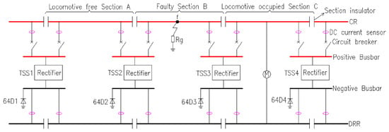
The DC traction power supply system for STM transit is illustrated in Figure 1.

Figure 1. Diagram of DC traction power supply system for STM transit.

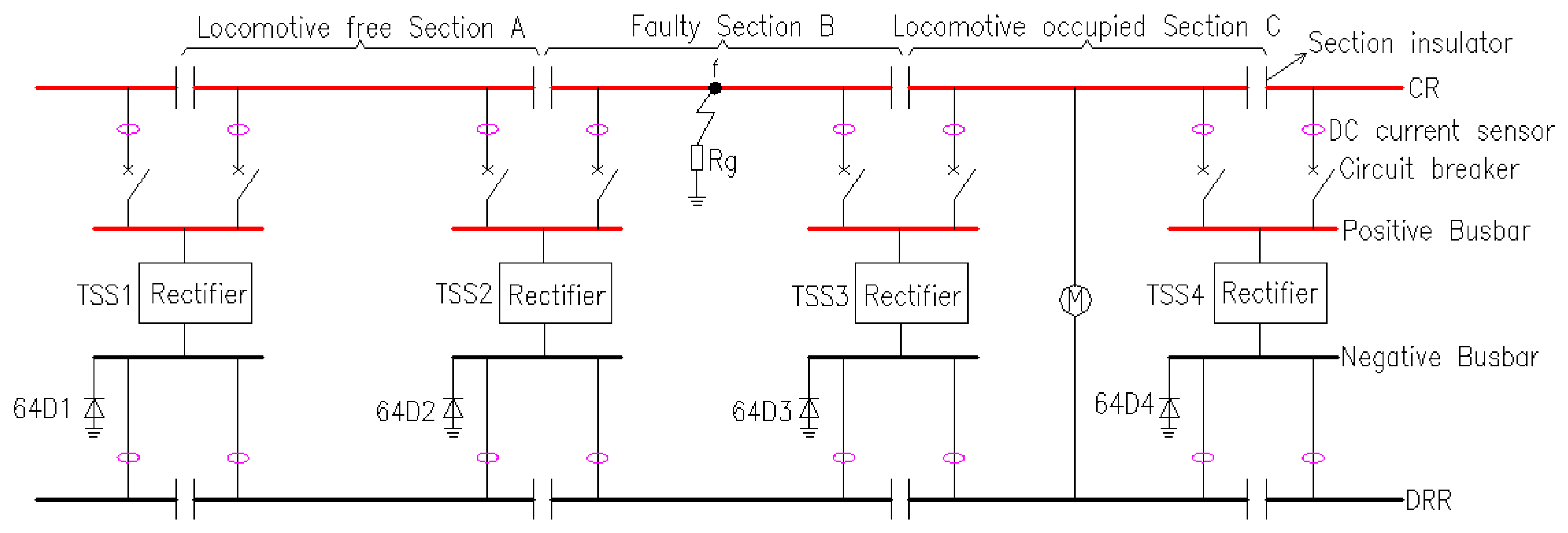
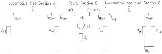
As illustrated in Figure 1, the system comprises four TSSs and three sections: locomotive-free zone A, fault zone B, and locomotive section C. DC current sensors are installed on both sides of the CR and DRR in each section. Negative busbars of each TSS are equipped with a 64D grounding protection device. When a locomotive suddenly enters the right entrance of Section C, or a grounding fault occurs at point f on the positive side of the CR in Section B via TR R_g, both cases lead to abrupt variations in the currents on both sides of the corresponding section, thereby generating a fault component. This paper employs the principle of superposition to derive the equivalent circuit diagrams of the DCTS for an STM transit under the two scenarios described above. Furthermore, it analyzes the fault components on both sides of the CR and DRR in each section based on these equivalent circuit diagrams. When only considering the grounding fault at point f on the CR of Section B through the TR R_g the unidirectional conducting devices within the 64D units of every TSS will operate, and short-circuit current flows into the negative busbar. Derived from the principle of fault components [15,16], an equivalent model of the fault components is presented in Figure 2.

Figure 2. Equivalent model of the fault component in DCTS during PPGF.

The switching states of the rectifier and unidirectional protection devices and the equivalent parameters of the locomotive load are assumed constant over the analysis interval, so the network is treated as linearized therein.

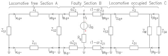
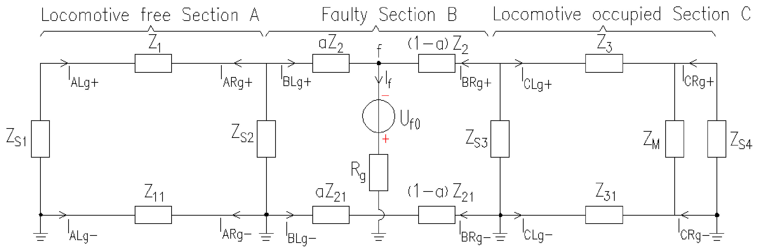
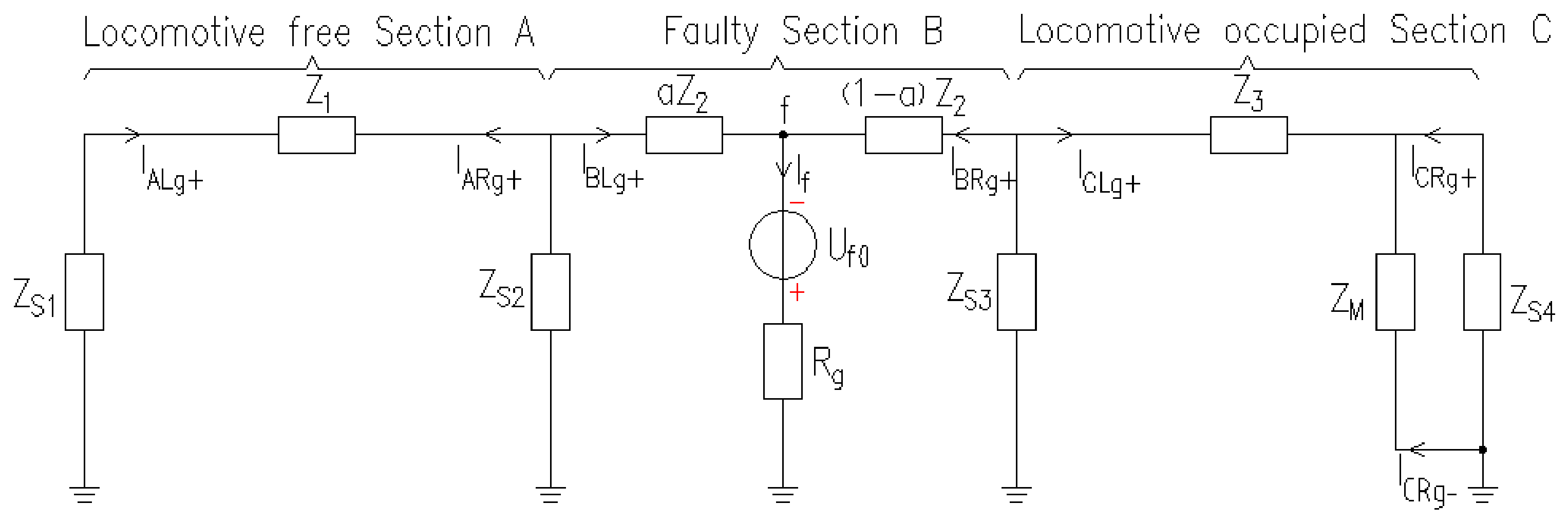
In Figure 2, Z₁, Z₂, and Z₃ are the equivalent impedances of the CRs in Sections A, B, and C, respectively; Z₁₁, Z₂₁, and Z₃₁ are the equivalent impedances of the DRRs in Sections A, B, and C, respectively; Z_S1, Z_S2, Z_S3, and Z_S4 are the equivalent impedances of TSSs 1, 2, 3, and 4, respectively; R_g denotes the TR at grounding point f on the positive pole of faulty Section B; Z_M is the equivalent impedance of the locomotive; U_f0 is the normal-state voltage at point f before the fault; I_ALg+, I_BLg+, and I_CLg+ are the fault components of the current on the left side of the CR in Sections A, B, and C, respectively; I_ARg+, I_BRg+, and I_CRg+ are the fault components of the current on the right side of the CR in Sections A, B, and C, respectively; I_ALg-, I_BLg-, and I_CLg- are the fault components of the current on the left side of the DRRs in Sections A, B, and C, respectively; I_ARg-, I_BRg-, and I_CRg- are the fault components of the current on the right side of the DRRs in Sections A, B, and C, respectively; I_f is the fault component of the short-circuit current flowing into fault point f; and α is the ratio of the distance from the PPGF point f to the left side of Section B to the total length of Section B. During a PPGF, the unidirectional diodes of type 64D in all TSSs conduct, so both terminals of the DRRs in each section maintain equal zero potential. No current flows through the branches containing Z₁₁, Z₂₁, and Z₃₁, so they can be treated as open circuits. Finally, a simplified equivalent model of the fault components is obtained, as shown in Figure 3.

Figure 3. Simplified equivalent model of the fault component in DCTS during PPGF.

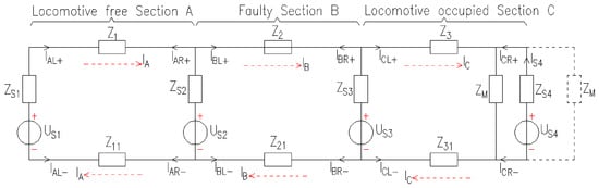
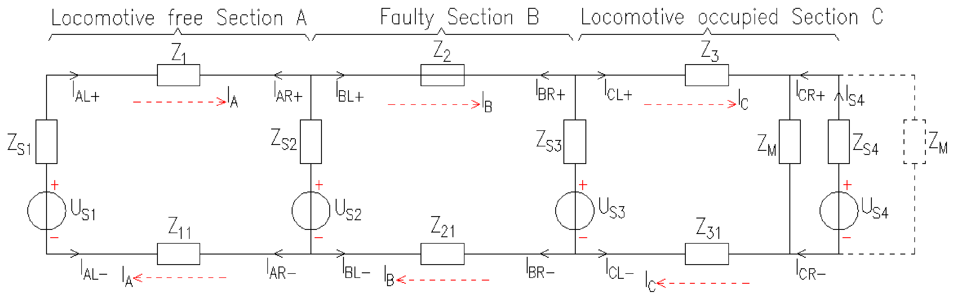
When only considering the sudden entry of a locomotive occurs on the right-hand entrance of Section C, the directions of the load currents measured at the right terminals of the CR and DRR of Section C reverse, while their magnitudes stay unchanged. By contrast, both the directions and magnitudes of load currents measured in other sections and at the left terminals of Section C remain constant. The corresponding equivalent model of DCTS is presented in Figure 4. In this figure, U_S1, U_S2, U_S3, and U_S4 represent the equivalent voltage sources of 1, 2, 3, and 4, respectively. I_AL+, I_BL+, and I_CL+ denote the currents at the left side of the CRs of Sections A, B, and C, respectively. I_AR+, I_BR+, and I_CR+ represent the currents on the right terminals of the CRs of Sections A, B, and C, respectively. I_AL−, I_BL−, and I_CL− denote the currents on the left terminals of the DRRs for Sections A, B, and C, respectively. I_AR−, I_BR−, and I_CR− denote the currents on the right terminals of the DRRs of Sections A, B, and C, respectively. I_A, I_B, and I_C represent the load currents flowing through Sections A, B, and C, respectively. I_S4 denotes the current flowing through the branch where U_S4 is located. The dashed line at Z_M indicates the position of the locomotive before it enters Section C, while the solid line at Z_M shows its position when the locomotive runs inside Section C.

Figure 4. Equivalent model of DCTS when the locomotive suddenly enters.

The traction locomotive with power electronic converters is essentially a constant-power load, whose apparent impedance varies with terminal voltage. In this paper, the fixed equivalent impedance Z_M is adopted as a small-signal approximation for fault incremental analysis, which is only valid at the instant of fault occurrence. At the moment of fault inception, the terminal voltage has not yet undergone large dynamic variation, and the locomotive operating point remains nearly unchanged. Therefore, the locomotive can be linearized to a constant impedance for extracting fault incremental components used in the protection criterion.

The above-mentioned linearized small-signal approximation has clear validity boundaries. It is only applicable to the initial transient instant after fault occurrence, where the voltage drop of the DC traction network is limited, and the operating point of the locomotive does not deviate drastically.

2.2. Characteristics of Fault Current Components Under a PPGF

When a PPGF occurs, this paper analyzes the characteristics of fault current components at both terminals of the CR and DRR in Sections A, B, and C based on Figure 3.

I.

Locomotive-Free Zone A

Based on Figure 3, the expressions for the fault current components on both sides of the positive rail and on both sides of the DRR in locomotive-free zone A can be derived, as shown in Equation (1).

$$\left\{\begin{array}{l}{\stackrel{.}{I}}_{\mathrm{AL}g+}=-{\stackrel{.}{I}}_{\mathrm{AR}g+}\\ {\stackrel{.}{I}}_{\mathrm{AL}g-}={\stackrel{.}{I}}_{\mathrm{AR}g-}=0\end{array}\right.$$

(1)

From Equation (1), the ASFCC at both terminals of the CR and DRR in locomotive-free Section A equals zero, as given in Equation (2).

$${\stackrel{.}{I}}_{\mathrm{AL}g+}+{\stackrel{.}{I}}_{\mathrm{AR}g+}+{\stackrel{.}{I}}_{\mathrm{AL}g-}+{\stackrel{.}{I}}_{\mathrm{AR}g-}=0$$

(2)

II.

Faulty Section B

The expressions for the fault current components at both terminals of the CR and DRR in faulty Section B can be derived from Figure 3, as presented in Equation (3).

$$\left\{\begin{array}{l}{\stackrel{.}{I}}_{\mathrm{BL}g+}+{\stackrel{.}{I}}_{\mathrm{BR}g+}={\stackrel{.}{I}}_{\mathrm{f}}\\ {\stackrel{.}{I}}_{\mathrm{BL}g-}={\stackrel{.}{I}}_{\mathrm{BR}g-}=0\end{array}\right.$$

(3)

It can be derived from Equation (3) that the ASFCC at both terminals of the CR and DRR in faulty Section B is equal to I_f, which denotes the total fault component current, as expressed in Equation (4).

$${\stackrel{.}{I}}_{\mathrm{BL}g+}+{\stackrel{.}{I}}_{\mathrm{BR}g+}+{\stackrel{.}{I}}_{\mathrm{BL}g-}+{\stackrel{.}{I}}_{\mathrm{BR}g-}={\stackrel{.}{I}}_{\mathrm{f}}$$

(4)

In Figure 3, the equivalent impedance on the left side of point f is Z_eqL, and that on the right side is Z_eqR. The values of the two impedances are given in Equation (5).

$$\left\{\begin{array}{l}{Z}_{\mathrm{eqL}}=\left(Z_{\mathrm{S}1}+Z_1\right)//Z_{\mathrm{S}2}+\alpha Z_2\\ Z_{\mathrm{eqR}}=\left[\left(Z_{\mathrm{M}}//Z_{\mathrm{S}4}+Z_3\right)//Z_{\mathrm{S}3}\right]+\left(1-\alpha \right)Z_2\end{array}\right.$$

(5)

From Figure 3 and Equation (5), the total fault component current I_f can be obtained, as shown in Equation (6).

$$I_f={\displaystyle \frac{U_{\mathrm{f}0}}{Z_{\mathrm{eqL}}{//Z}_{\mathrm{eqR}}+R_{\mathrm{g}}}}$$

(6)

The magnitudes of Z_S1, Z_S2, Z_S3, Z_S4, Z₁, Z₂, Z₃, and Z_M are relatively small and close to each other [17]. The value of α ranges from 0 to 1. It can be derived from Equation (5) that Z_eqL and Z_eqR are inductive with small magnitudes. Therefore, when the PPGF is not a metallic grounding fault, the magnitude of I_f is mainly determined by the TR R_g.

III.

Section C with the locomotive

The expressions for the fault current components at both terminals of the CR and DRR in Section C with the locomotive can be derived from Figure 3, as presented in Equation (7).

$$\left\{\begin{array}{l}{\stackrel{.}{I}}_{\mathrm{CL}g+}=-({\stackrel{.}{I}}_{\mathrm{CR}g+}+{\stackrel{.}{I}}_{\mathrm{CR}g-})\\ {\stackrel{.}{I}}_{\mathrm{CL}g-}=0\end{array}\right.$$

(7)

From Equation (7), it can be seen that the ASFCC at both terminals of the CR and DRR in Section C with the locomotive equals zero, as given in Equation (8).

$${\stackrel{.}{I}}_{\mathrm{CL}g+}+{\stackrel{.}{I}}_{\mathrm{CR}g+}+{\stackrel{.}{I}}_{\mathrm{CL}g-}+{\stackrel{.}{I}}_{\mathrm{CR}g-}=0$$

(8)

2.3. Characteristics of Fault Current Components When the Locomotive Suddenly Enters Section C

The load currents at both terminals of the CR and DRR in Sections A, B, and C are analyzed for the two working conditions: when the locomotive has not entered Section C, and when it suddenly enters Section C. This analysis is based on Figure 4, and the corresponding current fault components are then calculated.

I.

Load Current Conditions in the Event of the Locomotive Not Entering Section C

The situation in which the locomotive has not yet entered Section C is indicated by the dashed line in Figure 4, which shows the locomotive’s position. It can thus be concluded that the load currents on both sides of the CR in Sections A, B, and C, as well as on both sides of the DRR, can be determined. The expressions for the load currents on both sides of the CR and on both sides of the DRR in locomotive-free Section A are given in Equation (9).

$$\left\{\begin{array}{l}{\stackrel{.}{I}}_{\mathrm{AL}+}={\stackrel{.}{I}}_{\mathrm{AR}-}={\stackrel{.}{I}}_{\mathrm{A}}\\ {\stackrel{.}{I}}_{\mathrm{AL}-}={\stackrel{.}{I}}_{\mathrm{AR}+}=-{\stackrel{.}{I}}_{\mathrm{A}}\end{array}\right.$$

(9)

The expressions for load currents at both terminals of the CR and DRR in faulty Section B are presented in Equation (10).

$$\left\{\begin{array}{l}{\stackrel{.}{I}}_{\mathrm{BL}+}={\stackrel{.}{I}}_{\mathrm{BR}-}={\stackrel{.}{I}}_{\mathrm{B}}\\ {\stackrel{.}{I}}_{\mathrm{BL}-}={\stackrel{.}{I}}_{\mathrm{BR}+}=-{\stackrel{.}{I}}_{\mathrm{B}}\end{array}\right.$$

(10)

The expressions for load currents at both terminals of the CR and DRR in Section C with the locomotive are given in Equation (11).

$$\left\{\begin{array}{l}{\stackrel{.}{I}}_{\mathrm{CL}+}={\stackrel{.}{I}}_{\mathrm{CR}-}={\stackrel{.}{I}}_{\mathrm{C}}\\ {\stackrel{.}{I}}_{\mathrm{CL}-}={\stackrel{.}{I}}_{\mathrm{CR}+}=-{\stackrel{.}{I}}_{\mathrm{C}}\end{array}\right.$$

(11)

II.

Load Current Distribution When the Locomotive Suddenly Enters Section C

The solid line in Figure 4 represents the position of the locomotive after it suddenly enters Section C, from which the load currents at both terminals of the CR and DRR in Sections A, B, and C can be derived.

The load currents at both terminals of the CR and DRR in locomotive-free Section A are consistent with those in Equation (9).

The load currents at both terminals of the CR and DRR in faulty Section B remain the same as expressed in Equation (10).

The expressions for load currents at both terminals of the CR and DRR in Section C with the locomotive are provided in Equation (12).

$$\left\{\begin{array}{l}{\stackrel{.}{I}}_{\mathrm{CL}+}={\stackrel{.}{I}}_{\mathrm{C}}=-{\stackrel{.}{I}}_{\mathrm{CL}-}\\ {\stackrel{.}{I}}_{\mathrm{CR}+}={\stackrel{.}{I}}_{\mathrm{S}4}=-{\stackrel{.}{I}}_{\mathrm{CR}-}\end{array}\right.$$

(12)

III.

Characteristics of Fault Current Components When the Locomotive Suddenly Enters Section C

The fault current components at both terminals of the CR and DRR in Sections A, B, and C when a locomotive suddenly enters Section C can be calculated from Equations (9)–(12).

The fault current components at both terminals of the CR and DRR in locomotive-free Section A and faulty Section B are expressed in Equation (13).

$$\left\{\begin{array}{l}{\stackrel{.}{I}}_{\mathrm{AL}g+}={\stackrel{.}{I}}_{\mathrm{AR}g+}={\stackrel{.}{I}}_{\mathrm{AL}g-}={\stackrel{.}{I}}_{\mathrm{AR}g-}=0\\ {\stackrel{.}{I}}_{\mathrm{BL}g+}={\stackrel{.}{I}}_{\mathrm{BR}g+}={\stackrel{.}{I}}_{\mathrm{BL}g-}={\stackrel{.}{I}}_{\mathrm{BR}g-}=0\end{array}\right.$$

(13)

The fault current components on both sides of the CR and the DRR in locomotive-equipped Section C are shown in Equation (14).

$$\left\{\begin{array}{l}{\stackrel{.}{I}}_{\mathrm{CL}g+}={\stackrel{.}{I}}_{\mathrm{CL}g-}=0\\ {\stackrel{.}{I}}_{\mathrm{CR}g+}=-{\stackrel{.}{I}}_{\mathrm{CR}g-}={\stackrel{.}{I}}_{\mathrm{C}}+{\stackrel{.}{I}}_{\mathrm{S}4}\end{array}\right.$$

(14)

According to Equations (13) and (14), it can be derived that the algebraic sums of fault current components on both sides of the CR and the DRR in Sections A, B, and C are all zero, as shown in Equation (15).

$$\left\{\begin{array}{l}{\stackrel{.}{I}}_{\mathrm{AL}g+}+{\stackrel{.}{I}}_{\mathrm{AR}g+}+{\stackrel{.}{I}}_{\mathrm{AL}g-}+{\stackrel{.}{I}}_{\mathrm{AR}g-}=0\\ {\stackrel{.}{I}}_{\mathrm{BL}g+}+{\stackrel{.}{I}}_{\mathrm{BR}g+}+{\stackrel{.}{I}}_{\mathrm{BL}g-}+{\stackrel{.}{I}}_{\mathrm{BR}g-}=0\\ {\stackrel{.}{I}}_{\mathrm{CL}g+}+{\stackrel{.}{I}}_{\mathrm{CR}g+}+{\stackrel{.}{I}}_{\mathrm{CL}g-}+{\stackrel{.}{I}}_{\mathrm{CR}g-}=0\end{array}\right.$$

(15)

2.4. Analysis of Characteristics of Fault Current Components

I.

Only PPGF is Considered

According to the analysis in Section 2.2, under the fault condition with only a PPGF, the ASFCC at both terminals of the CR and the DRR in locomotive-free Section A and locomotive-equipped Section C equals zero. In contrast, the algebraic sum of fault current components at both terminals of the CR and the DRR in faulty Section B is equal to I_f.

II.

Only the Scenario Where the Locomotive Suddenly Enters is Considered

According to the analysis in Section 2.3, under the normal condition where only the locomotive suddenly enters, the ASFCC at both terminals of the CR and the DRR in locomotive-free Section A, faulty Section B, and locomotive-equipped Section C all equal zero.

III.

Simultaneous Occurrence of PPGF and the Locomotive Sudden Enters

When the PPGF and the sudden entry of the locomotive take place simultaneously, based on the circuit superposition theorem, the algebraic sum of fault current components at both terminals of the CR and the DRR in locomotive-free Section A and locomotive-equipped Section C is zero, while the algebraic sum of fault current components at both terminals of the CR and the DRR in faulty Section B is equal to I_f.

From the analysis of the above three working conditions, the amplitude characteristics of the algebraic sum of fault current components at both terminals of the CR and DRR in Sections A, B, and C are summarized as follows:

(1)

Once a PPGF occurs, the ASFCC at both terminals of the CR and DRR in faulty Section B equals I_f, while the ASFCC in all other sections is zero;

(2)

The amplitude of the total fault current component I_f is relatively large, but dominated by the TR;

(3)

Under normal operating conditions or when the locomotive suddenly enters the section, the algebraic sum of fault current components at both terminals of the CR and DRR in all sections is zero.

3. Principle of FSL for PPGF

3.1. Localization Principle of Fault Sections

As stated in Section 2.4, only the section with a PPGF has a non-zero M-ASFCC measured at both sides of the CR and DRR, while the M-ASFCC of all other sections is equal to zero. Therefore, this paper takes the M-ASFCC of feeder currents as the criterion for locating the PPGF section.

Firstly, calculate the ASFCC at both terminals of the CR and DRR within each section, denoted as I_g. Then compare its magnitude I_g with the setting current I_set for fault section identification. If |I_g| ≥ I_set, the corresponding section is identified as the faulty section with PPGF; if |I_g| < I_set, the section is judged to be under normal operating state. The FSL criterion is expressed in Equation (16).

$$\left\{\begin{array}{l}{I}_g=I_{\mathrm{Lg}+}+I_{\mathrm{Rg}+}+I_{\mathrm{Lg}-}+I_{\mathrm{Rg}-}\\ \left|I_{\mathrm{g}}\right|\ge I_{\mathrm{set}}\end{array}\right.$$

(16)

3.2. Principle Implementation

From Equation (16), it can be seen that the specific values of I_Lg+, I_Rg+, I_Lg−, I_Rg−, and I_set are mandatory for comparative identification. Specifically, I_Lg+ and I_Rg+ are calculated based on current signals measured by DC current sensors installed at two terminals of the CR within each section, and I_Lg− and I_Rg− are derived from sampling data obtained from DC current sensors on both terminals of the DRR. The magnitude of the setting current I_set shall be determined through comprehensive theoretical analysis.

One core criterion governs the selection of I_set: the DCTS shall avoid false identification under normal operation and fail-to-operate events when faults occur. Two constraints are thus taken into consideration. First, load current fluctuations and sampling deviations of DC current sensors under normal operating conditions will produce a non-zero magnitude |I_g| of the ASFCC at rail terminals. To prevent misjudgment of the FSL program, I_set should be set larger than the maximum value |I_g,max| of such spurious fault components. Second, I_set cannot exceed the minimum value I_f,min of total fault current components generated by PPGF, which ensures that the FSL program avoids missed judgment. The value constraint of I_set is given in Equation (17).

$$\left|I_{\mathrm{g}.\max }\right|\le I_{\mathrm{set}}<I_{\mathrm{f}.\min }$$

(17)

During normal operation, the transformation error among different DC current sensors is approximately 0.25% [18]. Let I_M denote the sum of rated currents of all locomotives on the feeder, and the maximum magnitude |I_g,max| can be calculated as expressed in Equation (18).

$$\left|I_{\mathrm{g}.\max }\right|=I_{\mathrm{M}}\times 2\times 0.25\%$$

(18)

When a PPGF occurs, it can be known from Equation (6) that I_f is closely correlated with the TR R_g. The value range of I_f is given in Equation (19).

$$0\le I_{\mathrm{f}}\le {\displaystyle \frac{U_{\mathrm{f}0}}{Z_{\mathit{eq}\mathrm{L}}{//Z}_{\mathit{eq}\mathrm{R}}}}$$

(19)

To guarantee the feasibility of the proposed algorithm and its capacity to withstand a certain TR, the minimum fault current component I_f,min is set to 1.2 × I_set. I_set is determined based on |I_g,max| with a certain safety margin, and the reliability coefficient is taken as 1.2. The formula for I_set is given in Equation (20). The maximum TR that can be tolerated by the algorithm proposed in this paper is expressed in Equation (21).

$$I_{\mathrm{set}}=1.2\times \left|I_{\mathrm{g}.\max }\right|=0.6\%\times I_{\mathrm{M}}$$

(20)

$$R_{\mathrm{g}.\max }={\displaystyle \frac{U_{\mathrm{f}0}}{1.2\times 0.6\%\times I_{\mathrm{M}}}}-Z_{\mathrm{eqL}}//Z_{\mathrm{eqR}}$$

(21)

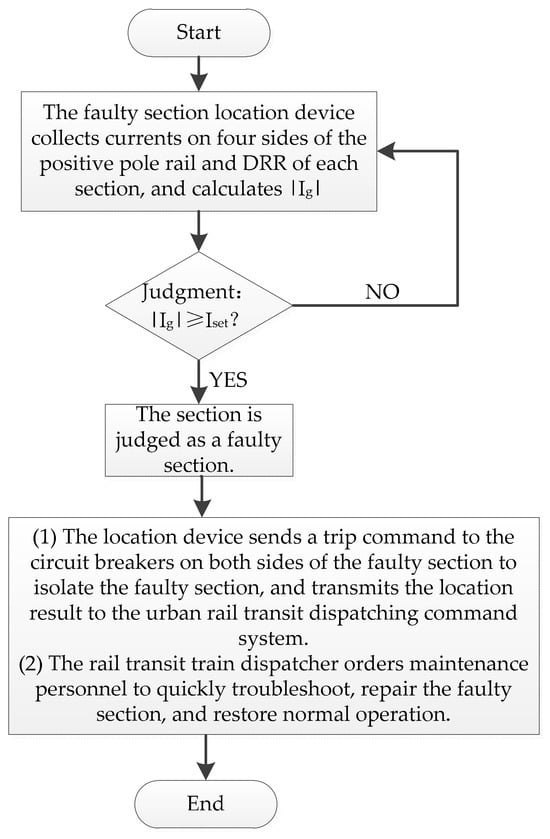
One FSL device is installed in each section. The detailed implementation procedure is described in four steps as follows:

(1)

Set the current setting value I_set of the FSL device according to Equation (20);

(2)

The FSL device collects feeder current data in real time via DC current sensors at both terminals of the CR and DRR within the section, and calculates the magnitude of feeder ASFCC, denoted as |I_g|;

(3)

Conduct real-time comparison between |I_g| and the setting current I_set. If |I_g| < I_set, the section is identified as a normal section; if |I_g| ≥ I_set, the section is identified as a faulty section;

(4)

For the identified faulty section, the FSL device sends trip signals to the circuit breakers on both sides to isolate the faulty section. The localization result is uploaded to the urban rail transit dispatch and control system. Then the rail transit dispatcher arranges maintenance staff to rapidly troubleshoot, repair the fault, and restore normal operation.

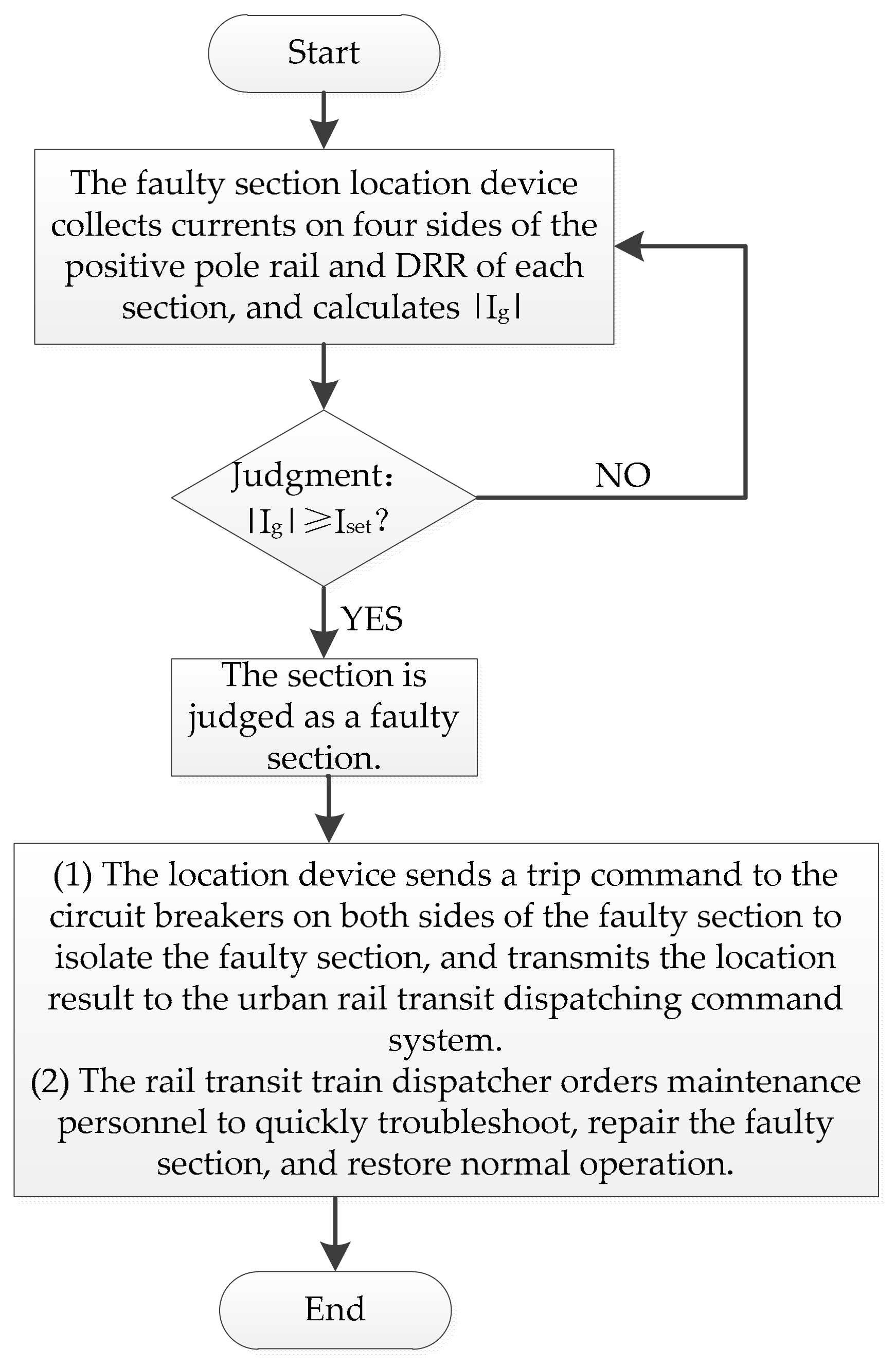
The flowchart of the proposed FSL algorithm is shown in Figure 5.

Figure 5. Flowchart of the FSL algorithm.

4. Simulation

4.1. Simulation Model

According to the STM transit DC traction power supply system schematic shown in Figure 1, a corresponding simulation model is established on the MATLAB/Simulink platform [19]. The DC rated supply voltage is 1500 V, and the feeder lengths of locomotive-free Section A, faulty Section B, and locomotive-equipped Section C are all set to 3 km [20]. The rated power of the locomotive is 180 kW, the inverter efficiency is 95%, and the rated power of the overall DCTS is 2000 kW. The setting current I_set of the proposed algorithm is calculated by Equation (20): I_set = 0.6% × 180/(1500 × 0.95) = 0.76 A ≈ 1 A. Thus, I_set is set to 1 A. The main simulation parameters are listed in Table 1. The relay setting resolution is only to the nearest integer.

Table 1. Simulation model parameters in MATLAB/Simulink.

No.	Parameter	Value
1	CR resistance r1/(Ω/km) DDR resistance r2/(Ω/km)	0.0128 [17]
2	CR inductance l1/(mH/km) DDR inductance l2/(mH/km)	0.25 [17]
3	equivalent resistance of 64D earthing relay R64D/(Ω)	5.0 [7]
4	rectifier transformer rated capacity S/(kVA)	500
5	locomotive rated power PM/(kW)	180 [20]
6	rated primary and secondary voltages of rectifier transformer U1/U2 (kV)	35/1.180 [21]
7	percentage short-circuit impedance of rectifier transformer Uk %	8% [21]

In this simulation, the traction locomotive is equivalently represented by a constant impedance ZM based on the small-signal linearization assumption at that fault instant. The simulation reproduces transient behaviors only at the initial moment after fault occurrence and ignores closed-loop dynamic adjustment of the locomotive inverter under sustained fault conditions.

To verify the correctness and effectiveness of the FSL method proposed in Section 3, a PPGF is arranged at the midpoint of Section B with a TR of 0Ω. Three working conditions are simulated and validated separately: pure PPGF, the locomotive suddenly enters, and the simultaneous occurrence of both events. The overall simulation duration is 0.14 s, starting at 0 s. Both the PPGF and the sudden locomotive entry occur at 0.1 s. The sampling cycle is 20 ms, with 70 sampling points per cycle [22].

4.2. Simulation Verification Under PPGF

A PPGF is set at the midpoint of Section B with a TR of 0 Ω. The M-ASFCC |I_g| for Sections A, B, and C are obtained from the simulation, as listed in Table 2. Only the magnitude of Section B exceeds the setting current I_set, while the magnitudes of Sections A and C are both lower than I_set. Accordingly, the PPGF is correctly identified within Section B.

Table 2. The M-ASFCC in each section during PPGF.

Line Section	M-ASFCC (A)	Judgment Result
A	0	Normal section
B	1086	Fault section
C	0	Normal section

4.3. Simulation Verification Under Sudden Locomotive Entry

A locomotive is set to suddenly enter the right inlet of Section C from the outside right side of Section C. The M-ASFCC |I_g| for Sections A, B, and C are obtained via simulation, as listed in Table 3. The magnitudes of all three sections are less than the setting current I_set, confirming that Sections A, B, and C are all correctly identified as being under normal operating conditions.

Table 3. The M-ASFCC in each section when the locomotive suddenly enters.

Line Section	M-ASFCC (A)	Judgment Result
A	0	Normal section
B	0	Normal section
C	0	Normal section

4.4. Simulation Verification Under Simultaneous PPGF and Sudden Locomotive Entry

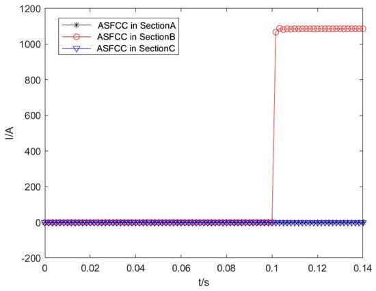
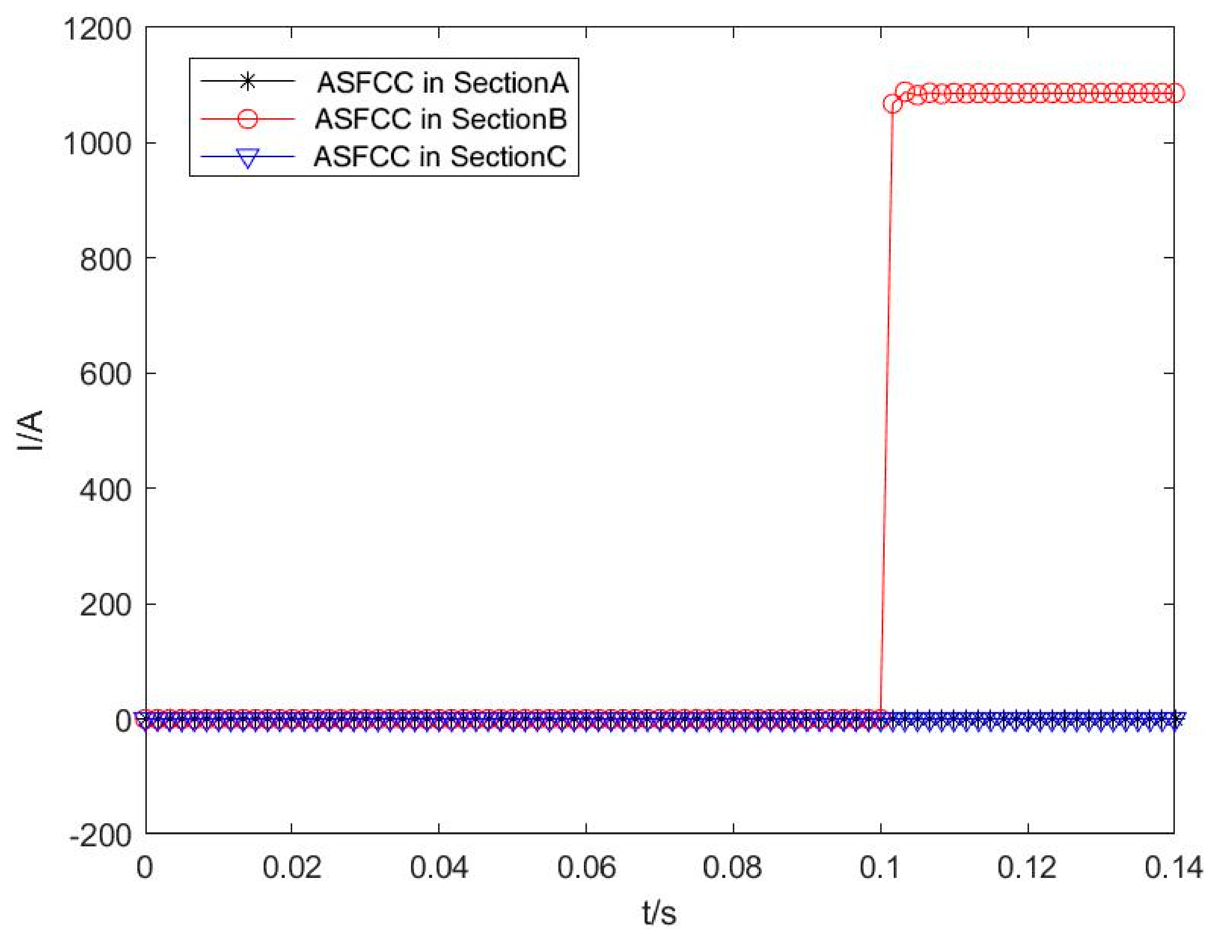
When a PPGF (consistent with the fault condition in Section 4.2) and a locomotive suddenly enter (consistent with the working condition in Section 4.3) simultaneously, the waveforms of the ASFCC for Sections A, B, and C are obtained by simulation, as illustrated in Figure 6. The results show that only the M-ASFCC of Section B is greater than the setting current I_set, while the M-ASFCC values of Sections A and C are both less than I_set. Thus, the PPGF is accurately localized to Section B.

Figure 6. Waveforms of ASFCC in each section when two conditions occur simultaneously.

4.5. Adaptability Analysis of the Proposed Scheme

Taking the simultaneous occurrence of a PPGF and locomotive sudden entry as the test condition, the adaptability of the proposed FSL method is analyzed. First, the performance is investigated under variable PPGF TR, different fault locations, and sampling delays. Next, a comparative study is conducted with the method presented in reference [14]. Finally, further adaptability verification is carried out by applying the method to a complex network structure.

(1)

Influence of TR

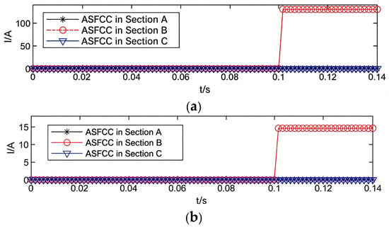
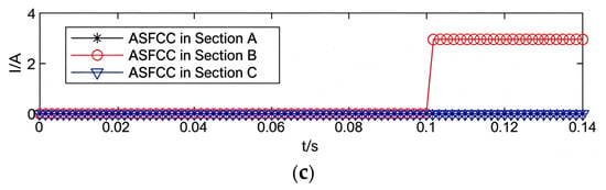
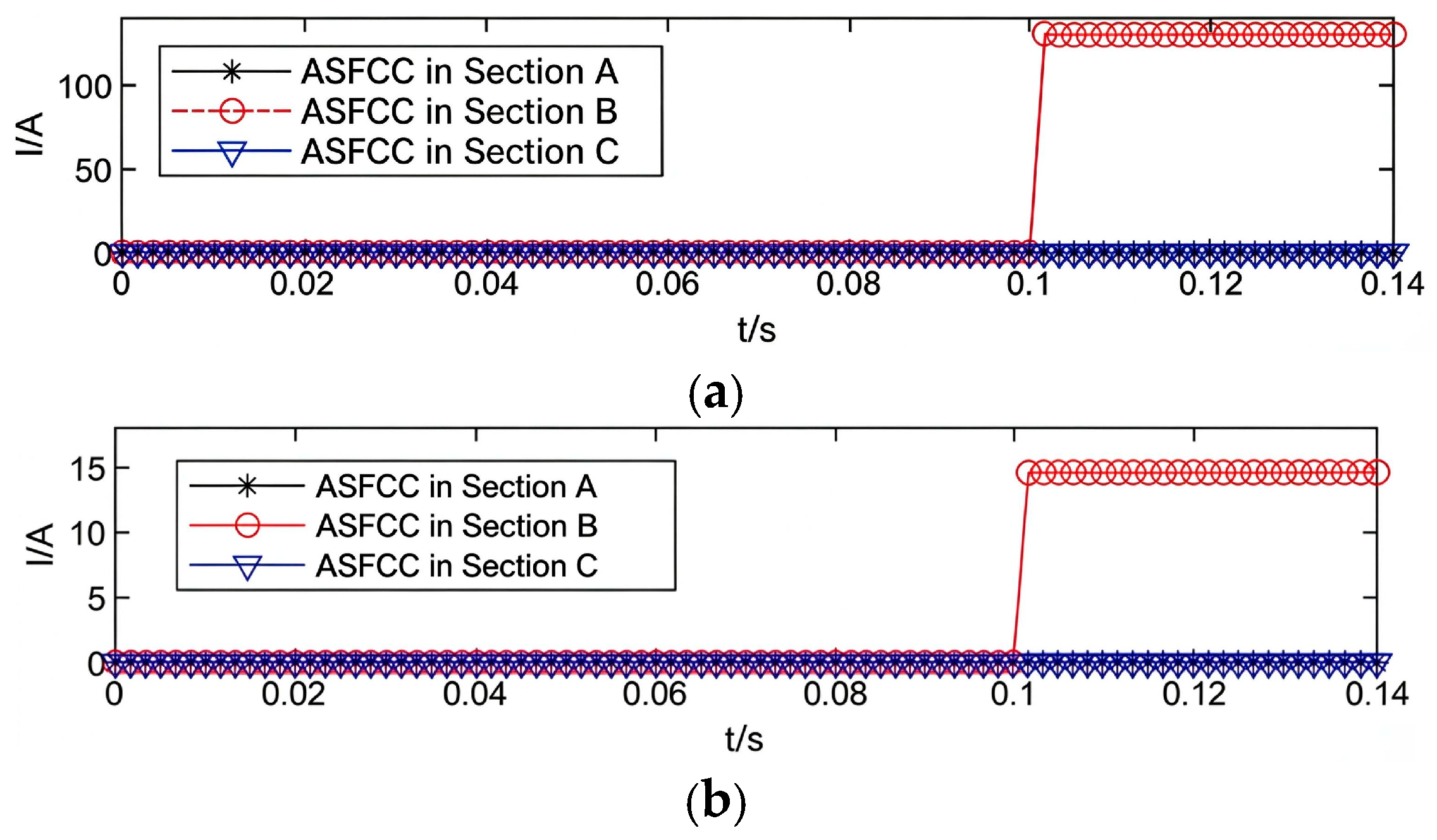
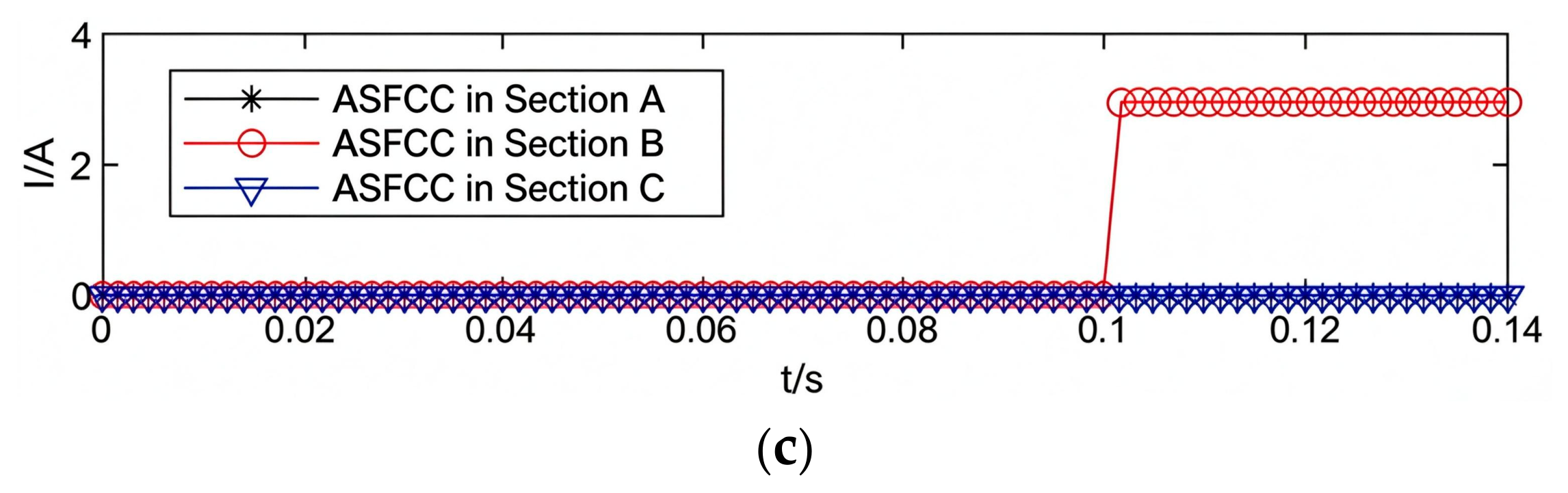
The PPGF is set at the midpoint of Section B, with the TR R_g configured as 10 Ω, 100 Ω, and 500 Ω, respectively. The simulated waveforms of ASFCC for Sections A, B, and C are shown in Figure 7.

Figure 7. Waveforms of ASFCC in each section under different TR values. (a) Waveforms of ASFCC in each section when the TR = 10 Ω. (b) Waveforms of ASFCC in each section when the TR = 100 Ω. (c) Waveforms of ASFCC in each section when the TR = 500 Ω.

It can be seen from Figure 7 that the magnitude of the algebraic sum of fault current components of Section B decreases with the increase in TR, while those of Section A and Section C remain 0 A at all times. When the TR reaches up to 500 Ω, the M-ASFCC of Section B is approximately 2.96 A, which exceeds the setting value of 1 A. The faulty section can be accurately identified without any adverse impact on the localization performance of the proposed method, which demonstrates that the algorithm has a strong capacity to withstand high TR.

(2)

Influence of Fault Location

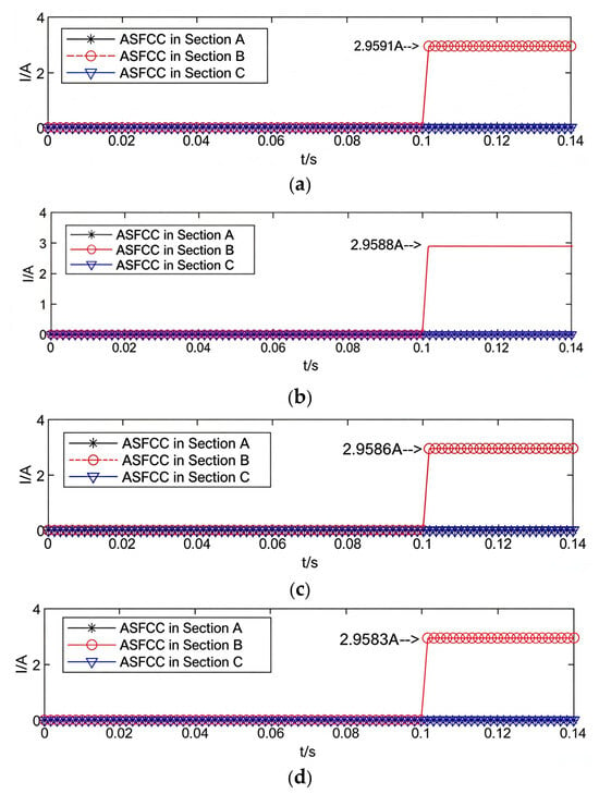
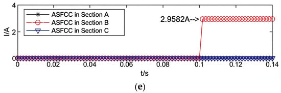
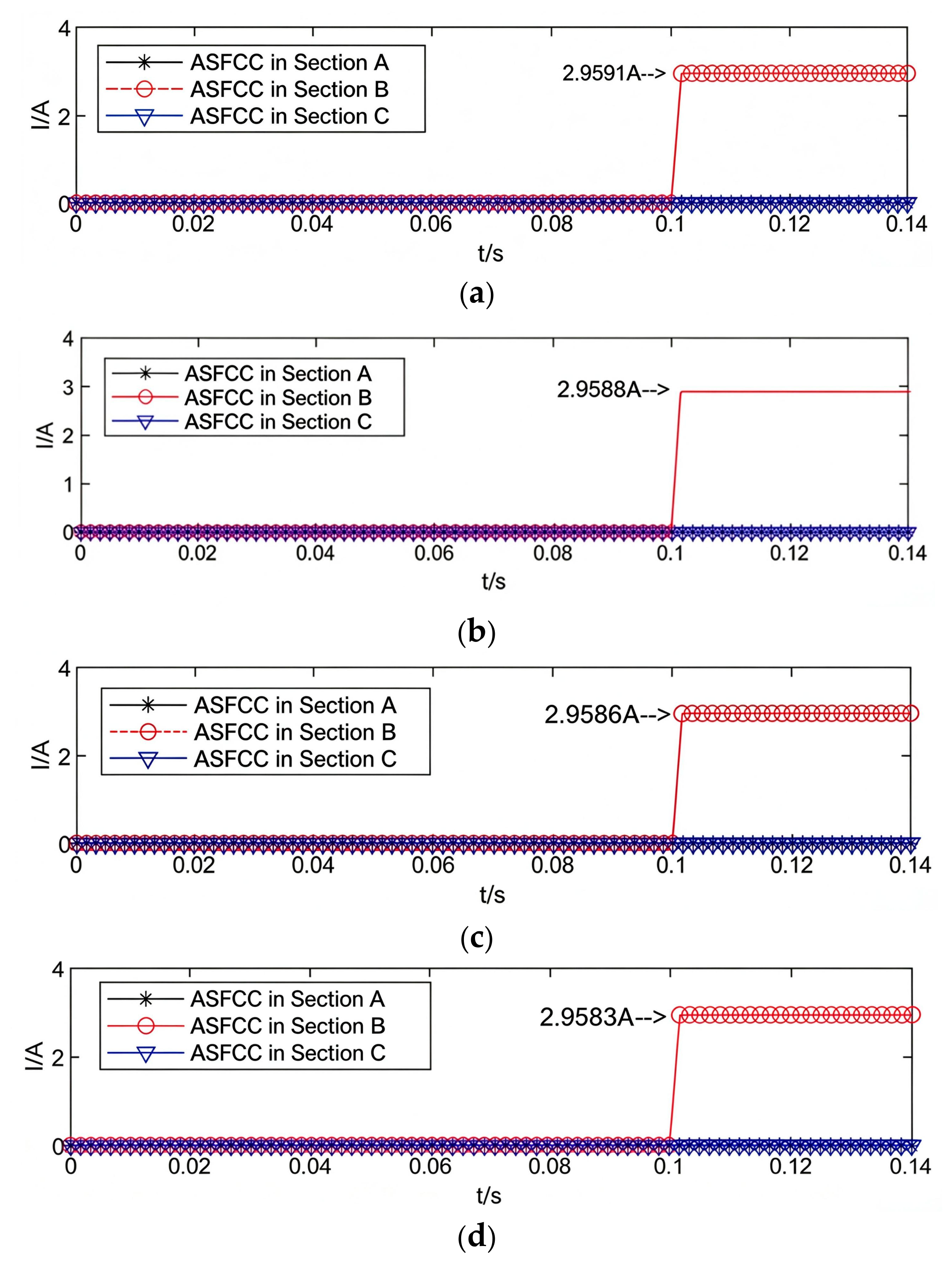
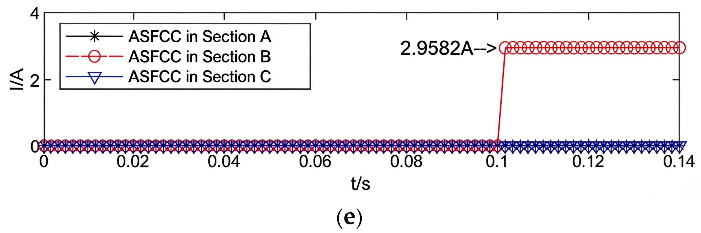
With the TR R_g set to 500 Ω, PPGF is separately set at five positions of Section B: at the start, 25% along the length, midpoint, 75% along the length, and at the terminal end. The waveforms of ASFCC for Sections A, B, and C are obtained via simulation, as shown in Figure 8.

Figure 8. Waveforms of ASFCC in each section at different fault locations. (a) Waveforms of the ASFCC in each section when the fault occurs at the head. (b) Waveforms of ASFCC in each section when the fault occurs at the 25% position. (c) Waveforms of ASFCC in each section when the fault occurs at the midpoint. (d) Waveforms of ASFCC in each section when the fault occurs at the 75% position. (e) Waveforms of ASFCC in each section when the fault occurs at the tail end.

It can be observed from Figure 8 that as the fault location varies, the M-ASFCC in Section B remains nearly constant, which is attributed to the extremely low impedance of the CR. The magnitude is approximately 2.96 A, exceeding the 1 A setting current, so the faulty section can be accurately identified. Meanwhile, the magnitudes of the algebraic sums in Sections A and C remain 0 A at all times, resulting in no false judgments for the normal sections. This demonstrates that the localization performance is barely affected by fault location, and its influence can be neglected.

(3)

Effect of Sampling Delay

The FSL device collects currents from both ends of each section. When the TR is set to 500 Ω and a sampling delay exists for the current on one side, the magnitudes of the ASFCC of Sections A, B, and C are obtained through simulation, as shown in Table 4. It can be found that the proposed method can accurately identify the faulty section when the unilateral current sampling delay of the fault section is less than or equal to 9 ms.

Table 4. The M-ASFCC in each section when a sampling delay occurs in the faulty section.

Time Delay (ms)	Magnitude of the Algebraic Sum of Fault Current Components (A)			Judgment Result
	Section A	Section B	Section C
3	0	2.95	0	Fault Section: B
6	0	2.95	0	Fault Section: B
9	0	2.95	0	Fault Section: B

(4)

Comparison and Analysis of Different Algorithms

A comparative analysis is carried out between the method proposed in this paper and the algorithm presented in reference [14]. Based on the model illustrated in Figure 1, simulations are performed under identical operating conditions with varying TR values and fault locations. The M-ASFCC of each section under the proposed method, as well as the currents and magnitudes of positive and negative feeder lines of each section from the algorithm in reference [14], are calculated. By comparing the above results with the setting values of the respective algorithms, the accuracy of FSL is verified, and the sensitivities of the two schemes are compared.

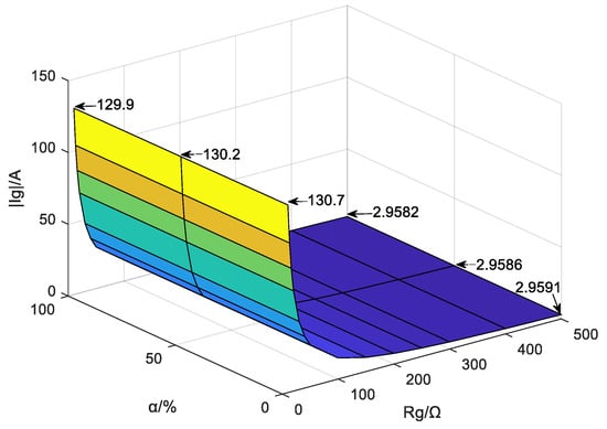
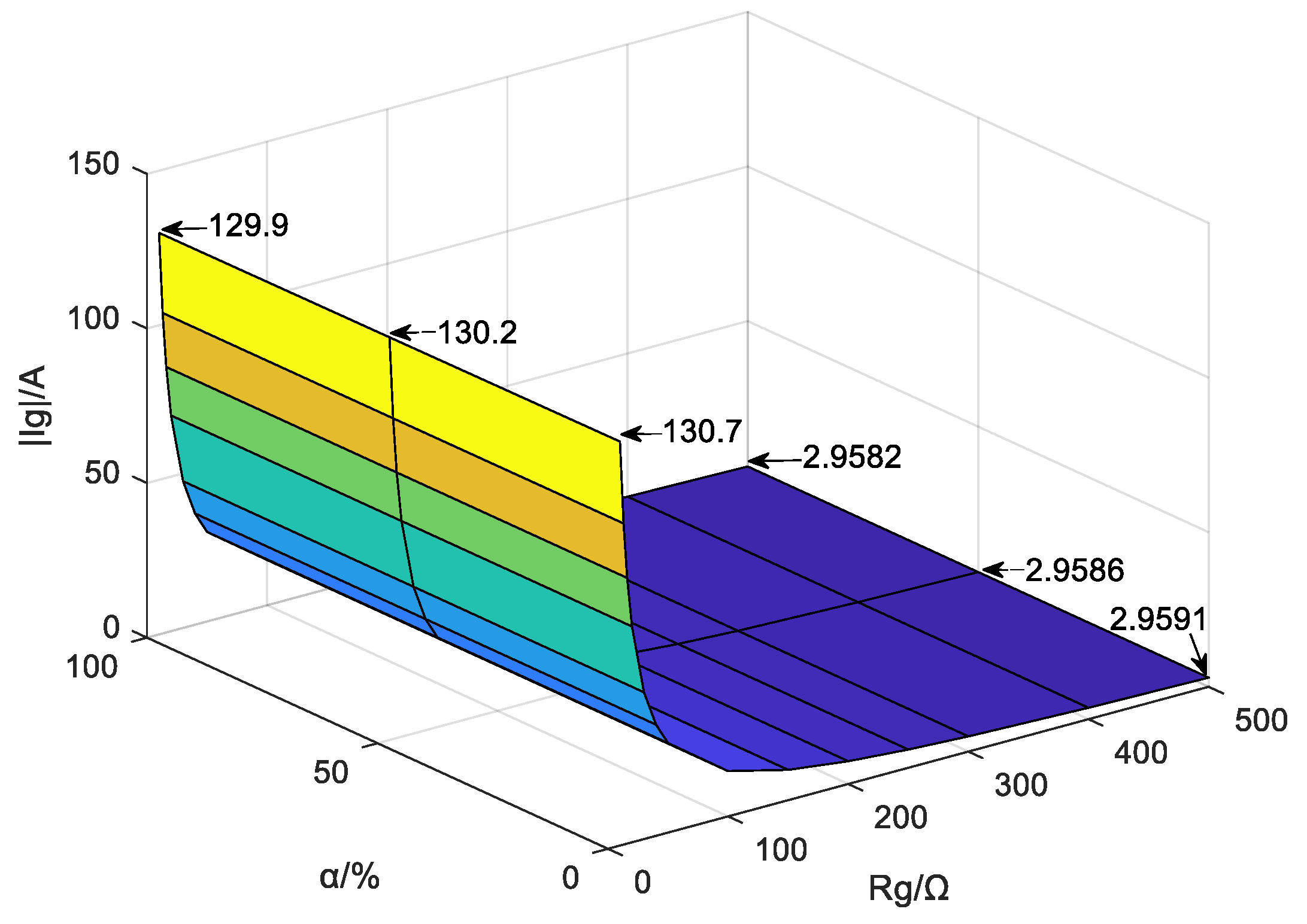
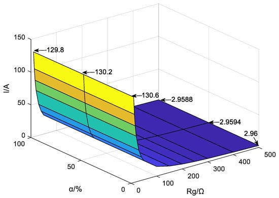
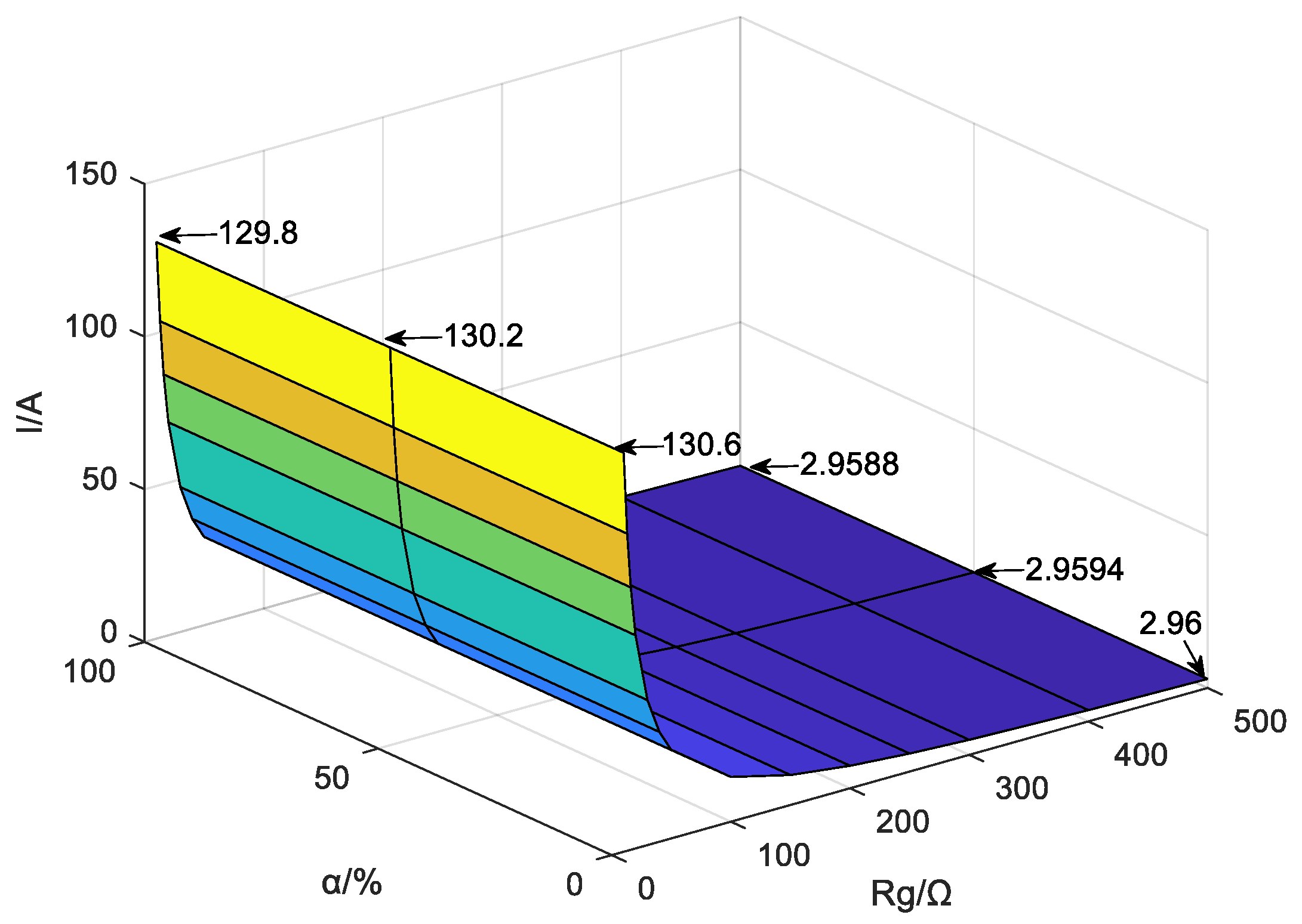
Fourteen groups of TR values are adopted, including 10 Ω, 13 Ω, 16 Ω, 20 Ω, 30 Ω, 40 Ω, 50 Ω, 100 Ω, 150 Ω, 200 Ω, 250 Ω, 300 Ω, 400 Ω, and 500 Ω. Simulations are conducted at three fault positions on Section B, namely the start, midpoint, and terminal end. The M-ASFCC in each section from the proposed method, as well as the currents and magnitudes of positive and negative feeder lines in each section from the algorithm in reference [14], are acquired. The index magnitudes of Section A and Section C obtained by both algorithms remain 0 A. The variation trends of the index magnitudes of Section B for the two algorithms are plotted in Figure 9 and Figure 10, respectively.

Figure 9. The algebraic sum amplitude of current fault components in the fault section of this article under different TR values at different positions.

Figure 10. The algebraic sum amplitude of current fault components in the fault section of reference [14] under different TR values at different positions.

It can be observed from Figure 9 and Figure 10 that the index magnitudes of Section B calculated by the two algorithms are roughly equal under various TR and fault positions. The index magnitude decreases with the increase of TR and declines as the fault position moves farther away. Compared with the fault position, TR exerts a more prominent influence on the index magnitude, which results from the low impedance of the CR and DRR.

In accordance with the parameters presented in Section 4.1, the setting value of the proposed method is calculated as 1 A, while that of the algorithm in reference [14] is 7 A. Different TR values led to distinct localization performance and sensitivity for the two algorithms, and the relevant results are summarized in Table 5.

Table 5. The effectiveness and sensitivity of two methods under different TR values.

TR (Ω)	Proposed Method		Algorithm in Reference [14]
	Judgment Performance	Sensitivity	Judgment Performance	Sensitivity
10	Accurate Judgment	130.25	Accurate Judgment	18.61
13	Accurate Judgment	103.72	Accurate Judgment	14.82
16	Accurate Judgment	85.89	Accurate Judgment	12.27
20	Accurate Judgment	69.78	Accurate Judgment	9.97
30	Accurate Judgment	47.46	Accurate Judgment	6.78
40	Accurate Judgment	35.96	Accurate Judgment	5.14
50	Accurate Judgment	28.94	Accurate Judgment	4.14
100	Accurate Judgment	14.65	Accurate Judgment	2.09
150	Accurate Judgment	9.81	Accurate Judgment	1.40
200	Accurate Judgment	7.37	Accurate Judgment	1.05
250	Accurate Judgment	5.90	Judgment Failure	0.84
300	Accurate Judgment	4.92	Judgment Failure	0.70
400	Accurate Judgment	3.70	Judgment Failure	0.53
500	Accurate Judgment	2.96	Judgment Failure	0.42

Data listed in the table indicate that when the TR equals 250 Ω, 300 Ω, 400 Ω, and 500 Ω, the proposed method achieves accurate faulty section localization, whereas the algorithm in reference [14] fails to identify the fault. For TR values of 10 Ω, 13 Ω, 16 Ω, 20 Ω, 30 Ω, 40 Ω, 50 Ω, 100 Ω, 150 Ω, and 200 Ω, both algorithms can accurately locate the faulty section, yet the sensitivity of the proposed algorithm is seven times that of the scheme in reference [14]. In comparison, the proposed method exhibits significant advantages in terms of tolerance to high TR and detection sensitivity.

(5)

Applicability of the Scheme Under Complex Topological Structures

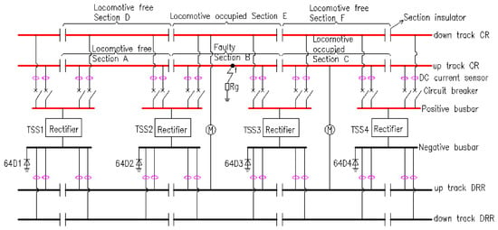
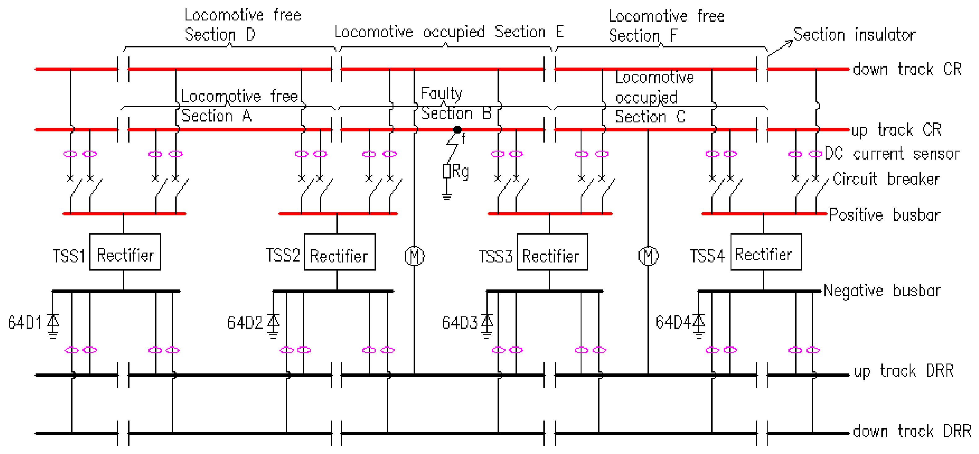
To further verify the applicability of the proposed scheme, the scheme is tested on a more complex topological structure. This topology is obtained by adding one feeder to the model in Figure 1 so as to build up-track and down-track circuits, as shown in Figure 11. The down-track circuit is split into three sections: locomotive-free Section D, locomotive-occupied Section E, and locomotive-free Section F. The parameters of the corresponding CR and DRR are identical to those of the up-track circuit.

Figure 11. Diagram of the DC traction power supply system for STM transit with up-track and down-track circuits.

Three working conditions are considered to occur simultaneously: a PPGF on Section B and the sudden entry of locomotives from the right side into Section C and Section E. The M-ASFCC for all sections is calculated via simulation to judge the operating state of each section. All simulation model parameters: the rated locomotive power, inverter efficiency, simulation time instant, total simulation duration, occurrence time of the PPGF, the moment of sudden locomotive entry, simulation sampling period, and sampling points per cycle are consistent with those provided in Section 4.1. The current setting value is calculated according to Equation (20): I_set = 0.6% × 180 × 2/(1500 × 0.95) = 1.52 A); I_set is taken as 2 A.

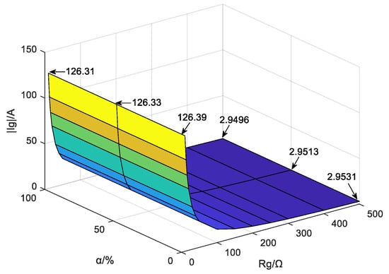
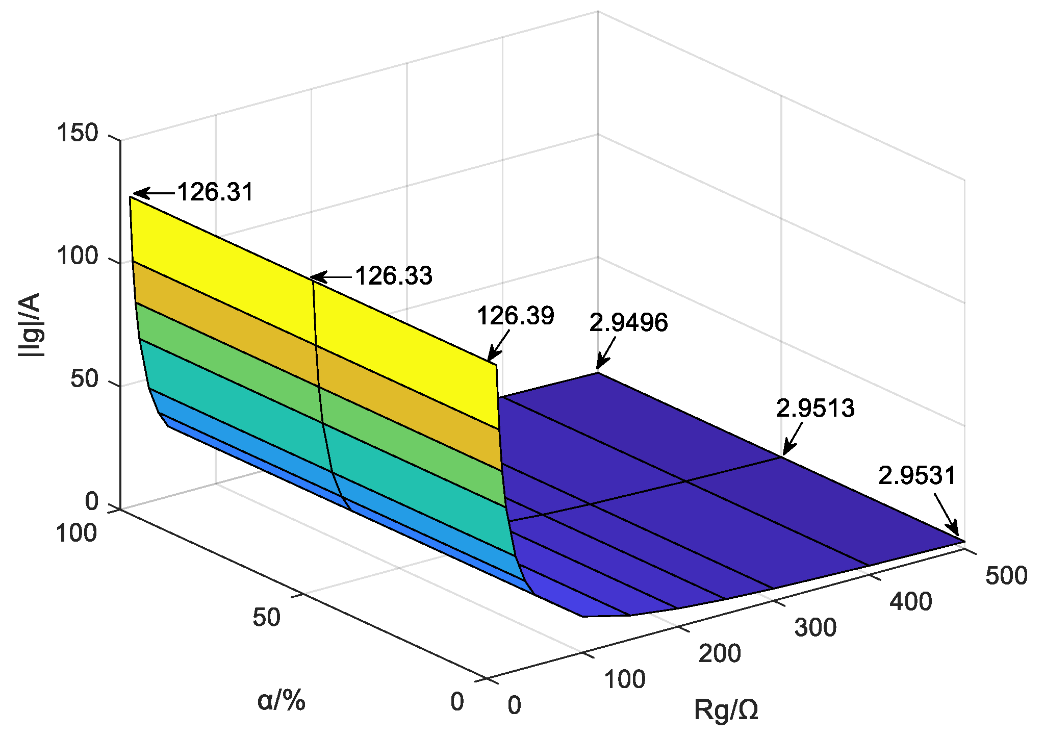
Fourteen groups of TR values are adopted, including 10 Ω, 13 Ω, 16 Ω, 20 Ω, 30 Ω, 40 Ω, 50 Ω, 100 Ω, 150 Ω, 200 Ω, 250 Ω, 300 Ω, 400 Ω, and 500 Ω. Simulations are carried out at the three fault positions of Section B, namely the start, midpoint, and terminal end. The variation of index magnitudes of Section B is illustrated in Figure 12.

Figure 12. The M-ASFCC in the fault section under different TR values at different positions in complex topological structures.

It can be observed from Figure 12 that the index magnitude of faulty Section B decreases as the TR rises, and it also declines when the fault position is farther away. Compared with the fault position, the TR has a more significant effect on the index magnitude. Under the extreme condition where the TR reaches 500 Ω and the fault point is located at the terminal end of Section B, the index magnitude of Section B still reaches 2.9496 A, which exceeds the setting value of 2 A with a sensitivity of 1.47. This enables reliable localization of faulty Section B. Under all working conditions, the index magnitudes of Section A, Section C, Section D, Section E, and Section F remain 0 A, so these sections can be accurately judged to be in normal operating states. Therefore, the proposed scheme can still accurately locate the faulty section under complex topological structures, which verifies that the method possesses satisfactory universality.

5. Conclusions

By analyzing the feeder fault current components under CR grounding faults and sudden locomotive access conditions in the STM transit DCTS, the following conclusions are drawn in this paper:

(1)

Equivalent models of fault components for the DCTS under PPGF and equivalent models for the DCTS with the locomotive suddenly entering are established, respectively. The characteristics of M-ASFCC on both sides of the CR and DRR of each section are analyzed under three operating scenarios, namely the independent PPGF, independent sudden locomotive entry, and simultaneous occurrence of the two conditions. A FSL method based on the M-ASFCC is proposed in this paper;

(2)

One FSL device is installed for each section. Feeder currents are collected in real time through DC current sensors arranged on both sides of the CR and DRR of the corresponding section. The M-ASFCC of this section is then calculated and compared with the setting value to determine the operating state of the section. The proposed method can accurately identify faulty sections under various fault positions and different TR. The M-ASFCC is slightly affected by fault positions, and such influence can be neglected. In contrast, it is greatly affected by TR, yet the method can withstand a TR of up to 500 Ω. Meanwhile, the scheme can effectively eliminate the interference caused by impact loads;

(3)

The theoretical derivation of the proposed method relies on the small-signal linearization assumption at that fault instant, where the constant-power locomotive load is simplified as a fixed impedance. This assumption holds only when the voltage disturbance of the traction network is moderate at fault inception. Theoretical error will be introduced under severe voltage collapse caused by long-duration faults or faults occurring directly within locomotive-occupied sections. All simulation cases in this paper are verified for the initial transient moment after fault occurrence;

(4)

Compared with the algorithm in reference [14], the FSL method proposed in this paper delivers superior localization performance, supports higher tolerable TR, and achieves higher algorithm sensitivity. This method is not only applicable to grounding fault localization of STM DCTS, but also provides technical support and a theoretical basis for faulty section diagnosis of other urban rail transit systems, including maglev and metro;

(5)

It is worth noting that all case studies in this paper are carried out via simulation. Further physical experiments on a hardware test platform will be conducted to advance the practical engineering deployment of the proposed method.

References

- Han, B.M.; Xi, Z.; Sun, Y.J. Statistical Analysis of Urban Rail Transit Operations in the World in 2022: A Review. Urban Rapid Rail Transit 2022, 35, 1–5. [Google Scholar] [CrossRef]
- Li, J.G. Illustrated Urban Rail Transit; China Machine Press: Beijing, China, 2016. [Google Scholar]
- Sun, J.J.; Lan, H.F.; Li, G.Y.; Pan, Z.; Liu, W. Stray Current Diffusion Model of Metro DC Traction Power Supply System and Its Suppression Measures. Urban Mass Transit 2026, 29, 54–60. [Google Scholar] [CrossRef]
- Gu, J.D.; Yang, X.F.; Zheng, Q.L.; Zuo, X.T.; Shang, Z.; Zhao, Z.J. Rail Potential and Stray Current on Negative Resistance Converter Traction Power System under Different Grounding Schemes and Train Conditions. Trans. China Electrotech. Soc. 2021, 36, 1703–1717. [Google Scholar] [CrossRef]
- Zhang, Y.T. Traction Power Supply Technology of Fourth-Rail Return for Urban Rail Transit. Mod. Urban Transit 2011, 4, 8–10. [Google Scholar] [CrossRef]
- Yan, N.N.; Wang, J.; Sun, J.X. Review of Research on Medium and Low Speed Maglev Transportation Grounding Systems. J. Electr. Eng. 2023, 18, 35–45. [Google Scholar] [CrossRef]
- Zhou, C.F. Earthing Protection Design of DC Traction System for Straddle Monorail Transit. Urban Rapid Rail Transit 2010, 23, 93–96. [Google Scholar]
- Wang, L.; Chen, J.L.; Zhang, B. Design of Grounding Protection for Straddle Type Monorail Car. Electr. Drive Locomot. 2018, 6, 111–114. [Google Scholar] [CrossRef]
- GB 50458-2022; Code for Design of Straddle Monorail Transit. Ministry of Housing and Urban-Rural Development of the People’s Republic of China: Beijing, China, 2022.
- Hao, Z.H. DC Traction Power Supply System Based on MATLAB Simulation. Master’s Thesis, Beijing Jiaotong University, Beijing, China, 2020. [Google Scholar]
- Huang, H. DC Ground Protection Scheme of Urban Rail Transit Special Return Rail System. Urban Mass Transit 2022, 25, 203–206, discussion 210. [Google Scholar] [CrossRef]
- Sun, C.Q. Analysis of Grounding Protection Scheme for Traction Power Supply System of Medium-Low Speed Maglev. Electr. Railw. 2018, 29, 81–82, discussion 86. [Google Scholar] [CrossRef]
- Wang, Z.R.; Xi, F.H. Research on Optimization and Improvement of Grounding Protection for Monorail Transit. Electr. Railw. 2020, 31, 118–120, discussion 124. [Google Scholar] [CrossRef]
- Liu, Y.S.; Hou, W.; Wang, X. Grounding Fault Protection for Traction Power Supply System with Dedicated Rail Return Based on Feeder Line and Current. Electr. Railw. 2024, 35, 53–56. [Google Scholar] [CrossRef]
- Ge, Y.Z. Principles and Techniques of New Type Relay Protection and Fault Location, 2nd ed.; Xi’an Jiaotong University Press: Xi’an, China, 2007. [Google Scholar]
- Chen, D.; Wu, L.M.; Lin, F.H. The Fault Location Method of DC Distribution Network. Electr. Switchg. 2018, 56, 23–25. [Google Scholar] [CrossRef]
- Zhang, J.L. Research on DC-Side Short-Circuit Fault of Metro Power Supply System. Master’s Thesis, Southwest Jiaotong University, Chengdu, China, 2011. [Google Scholar]
- Zhang, X.K.; Li, Q.; Huang, Y.; Liu, G.; Yuan, C. A Dual-Function Planar Magnetically Coupled Current Sensor for High-Frequency Oscillation Suppression and Switching Current Measurement. IEEE Trans. Power Electron. 2026, 41, 61–67. [Google Scholar] [CrossRef] [Scilit]
- Yu, Q.; Cao, N. MATLAB/Simulink Power System Modeling and Simulation, 2nd ed.; China Machine Press: Beijing, China, 2017. [Google Scholar]
- Shi, R.; Wang, R.R.; Zhang, D.R. Optimum Design of Current Incremental Protection Based on Train Load Characteristics. Urban Mass Transit 2019, 22, 79–81; discussion 84. [Google Scholar] [CrossRef]
- Guo, S.C.; Liu, Y.S.; Wu, J.; Hou, W.; Jiang, X.; Zhang, X.L.; Chen, K.; Shi, X.J. A Precise Identification Method for Fault Trains Based on Train Grounding Current. Electr. Power 2024, 57, 143–150. [Google Scholar] [CrossRef]
- Chen, L.H.; Hou, T.Y.; Zou, B.G. Research on Harmonic Characteristics of Low Voltage Distribution Network and Influence of Network Loss. Autom. Electr. Power Syst. 2021, 42, 41–45. [Google Scholar] [CrossRef]
Disclaimer/Publisher’s Note: The statements, opinions and data contained in all publications are solely those of the individual author(s) and contributor(s) and not of MDPI and/or the editor(s). MDPI and/or the editor(s) disclaim responsibility for any injury to people or property resulting from any ideas, methods, instructions or products referred to in the content. |
© 2026 by the authors. Licensee MDPI, Basel, Switzerland. This article is an open access article distributed under the terms and conditions of the Creative Commons Attribution (CC BY) license.