Inertial Self-Adaptive Viscosity Algorithm for Common Solution of Split Mixed Equilibrium, Split Variational Inclusion and Fixed Point Problems

Abstract

This study aims to propose a self-adaptive viscosity-type algorithm with inertial effects to find the common solutions of the split mixed equilibrium, split variational inclusion and common fixed point problems associated with nonexpansive mappings. It is worth mentioning that the step size employed in this algorithm is independent of the operator norm. Strong convergence of the sequence defined by the proposed algorithm is established. As a consequence, the proposed method can be employed to approximate solutions of the split minimization, split common null point and split feasibility problems. The efficiency of the proposed algorithm is validated by a numerical example and its performance is illustrated by graphical comparisons relative to various established methods presented in recent literature.

1. Introduction and Preliminaries

Nonlinear operator theory plays a key role in solving a wide range of problems such as ordinary and partial differential equations, control theory, optimization and fixed point problems. Over the past few years, considerable interest has focused on the development of numerical schemes to solve the nonlinear operator equations and inclusions, with emphasis on efficiency and ease of implementation and analysis.

Throughout this paper, $\mathbb{R}$ will denote the set of real numbers, while $\mathbb{N}$ is the set of natural numbers, where $\mathcal{Z},{\mathcal{Z}}_1,{\mathcal{Z}}_2$ denote real Hilbert spaces. Moreover, ${\mathcal{J}}_1$ and ${\mathcal{J}}_2$ are nonempty convex and closed subsets of ${\mathcal{Z}}_1$ and ${\mathcal{Z}}_2$, respectively. Let $A:{\mathcal{Z}}_1\to {\mathcal{Z}}_2$ be a bounded linear operator and $A^{*}$ its adjoint operator.

A mapping $S:{\mathcal{J}}_1\to {\mathcal{J}}_1$ is referred to as Lipschitz continuous, if we have a $\nu >0$ which satisfy $\parallel S{j}_1-S{j}_2\parallel \le \nu \parallel j_1-j_2\parallel$ for all $j_1,j_2\in {\mathcal{J}}_1$. If $\nu$ satisfies $0<\nu <1$, then S is called the contraction mapping. Moreover, if $\nu =1$, then S is known as a nonexpansive mapping. The set consisting of all the fixed points of the map S is represented by $\mathcal{F}\left(S\right)$.

Nonexpansive mappings are important for several reasons. For instance, the geometric characteristics of the underlying spaces play a crucial role in ensuring the existence of fixed points for these mappings. These mappings often appear as transition mappings in the study of initial value problems for differential equation and inclusions involving accretive mappings. Third, many problems arising in fields such as convex optimization, compressed sensing, variational and monotone inclusions and image restoration naturally lead to operator equations involving nonexpansive mappings (see [1,2]). In addition, nonexpansive mappings are also relevant in areas such as complex analysis, particularly in the study of mappings that are complex differentiable and the geometry of Hilbert ball (see for example, [3,4]).

It should be noted that the multivalued map $T:\mathcal{Z}\rightrightarrows \mathcal{Z}$ is said to be monotone, if we have $⟨j_1-j_2,j_3-j_4⟩\ge 0,$ for each $j_1,j_2\in \mathcal{Z}$ with $j_3\in T{j}_1$ and $j_4\in T{j}_2$. A monotone mapping T is maximal in case there is no other monotonic function that exists, and whose graph properly contains the graph of T.

If $\lambda >0$ and I are an identity mapping on $\mathcal{Z}$, then $J_{\lambda }^T={(I+\lambda T)}^{-1}$ is the resolvent of T.

A self operator S on $\mathcal{Z}$ is referred to as $\mu$-inverse strongly monotone ($\mu$-ISM) if $⟨S{j}_1-S{j}_2,j_1-j_2⟩\ge \mu {\parallel S{j}_1-S{j}_2\parallel }^2$ for some $\mu >0$ and for all $j_1,j_2\in \mathcal{Z}$. In cases where $\mu =1$, then S is known as ISM or firmly nonexpansive mapping.

Observe that, for any $j_1\in \mathcal{Z}$, we get a distinct $P_{{\mathcal{J}}_1}{j}_1\in {\mathcal{J}}_1$ with

$$\parallel j_1-P_{{\mathcal{J}}_1}{j}_1\parallel =\inf \{\parallel j_1-j_2\parallel :j_2\in {\mathcal{J}}_1\}.$$

The above property defines a mapping $P_{{\mathcal{J}}_1}:$$\mathcal{Z}\to {\mathcal{J}}_1$ called a metric projection on ${\mathcal{J}}_1$. It satisfies the following inequality:

$$\parallel P_{{\mathcal{J}}_1}{j}_1-P_{{\mathcal{J}}_1}{j}_2{\parallel }^2 \le ⟨P_{{\mathcal{J}}_1}{j}_1-P_{{\mathcal{J}}_1}{j}_2,j_1-j_2⟩,$$

(1)

for all $j_1,j_2\in \mathcal{Z}$. Further, for every $j_1\in \mathcal{Z}$, we have

$$P_{{\mathcal{J}}_1}{j}_1=j\mathrm{if}\mathrm{and}\mathrm{only}\mathrm{if}⟨j_1-j,j-j_2⟩\ge 0,\forall j_2\in {\mathcal{J}}_1,$$

(2)

and

$$\parallel j_1-P_{{\mathcal{J}}_1}{j}_1{\parallel }^2+\parallel j-P_{{\mathcal{J}}_1}{j}_1{\parallel }^2 \le {\parallel j_1-j\parallel }^2,\mathrm{for}\mathrm{all}{j}_1,j\in \mathcal{Z}.$$

(3)

For more discussion on the properties of projection mappings, one can see [5] and the Section 3 of [3].

Assume that S and T are self mapping on $\mathcal{Z}$. We denote FPP as fixed point problem which can be formulated as:

$$\mathrm{Find} j^{*}\in \mathcal{Z} \mathrm{which} \mathrm{satisfy} S{j}^{*}=j^{*}.$$

If $j^{*}=S{j}^{*}=T{j}^{*}$, then $j^{*}$ is known as the common fixed point of S and T.

If F is a mapping from ${\mathcal{J}}_1\times {\mathcal{J}}_1$ into $\mathbb{R}$, we denote EP as equilibrium problem for a mapping F which can be formulated as follows:

$$\mathrm{Find} j^{*}\in {\mathcal{J}}_1 \mathrm{which} \mathrm{satisfy} F(j^{*},j)\ge 0,\forall j\in {\mathcal{J}}_1.$$

The variational inequality problem (VIP) of mapping $\varphi$ from ${\mathcal{J}}_1$ into $\mathcal{Z}$ is given by:

$$\mathrm{Find} j^{*}\in {\mathcal{J}}_1 \mathrm{with} ⟨j-j^{*},\varphi j^{*}⟩\ge 0,\forall j\in {\mathcal{J}}_1.$$

Denote $MEP(F,\varphi )$ to the mixed equilibrium problem and it is formulated as follows:

$$\mathrm{Find}{j}^{*}\in {\mathcal{J}}_1\mathrm{with}F(j^{*},j)+⟨j-j^{*},\varphi j^{*}⟩\ge 0,\mathrm{holds}\mathrm{for}\mathrm{all}j\in {\mathcal{J}}_1.$$

(4)

If $\varphi =\mathbf{0}$ in (4), then $MEP(F,\varphi )$ becomes the EP. If $F=\mathbf{0}$ in (4), then $MEP(F,\varphi )$ reduces to VIP. Assume G is a mapping from ${\mathcal{J}}_2\times {\mathcal{J}}_2$ into $\mathbb{R}$ and $\phi :{\mathcal{J}}_2\to {\mathcal{Z}}_2$, then split mixed equilibrium problem $SMEP$ is expressed by:

$$\mathrm{Find}{j}^{*}\in {\mathcal{J}}_1\mathrm{which}\mathrm{satisfy}F(j^{*},j)+⟨j-j^{*},\varphi j^{*}⟩\ge 0,\mathrm{holds}\mathrm{for}\mathrm{all}j\in {\mathcal{J}}_1,$$

(5)

such that

$$A{j}^{*}\in {\mathcal{J}}_2\mathrm{with}G(A{j}^{*},j^{\prime })+⟨j^{\prime }-A{j}^{*},\phi \left(A{j}^{*}\right)⟩\ge 0,\mathrm{holds}\mathrm{for}\mathrm{all}{j}^{\prime }\in {\mathcal{J}}_2.$$

(6)

Note that, the $MEP(F,\varphi )$ is a special case of $SMEP$. Furthermore, EP, VIP, split EP, and split VIP are the particular cases of the $SMEP$ defined in (5) and (6). In fact, the $SMEP$ framework covers the whole system that contains many problems such as complementarity, optimization, fixed point and the Nash equilibrium problems (see [6,7,8,9]). From now onward, a set $\Gamma$ denotes the solution set of $SMEP$.

Many researchers have given considerable attention to the split inverse problem (SIP). One of its earliest and most-studied forms is the split feasibility problem (SF) [10]. The SF related to $A:{\mathcal{Z}}_1\to {\mathcal{Z}}_2$ is stated as:

$$\mathrm{Find} j^{*}\in {\mathcal{J}}_1 \mathrm{such} \mathrm{that} A{j}^{*}\in {\mathcal{J}}_2.$$

This problem has important applications in various practical fields including signal and image processing and a radiotherapy technique based on intensity modulation and in other fields. For more developments and results in this direction, see [11,12,13,14,15,16].

Another problem called split inverse problem (SIP) is stated as:

$$\mathrm{Find} j^{*}\in {\mathcal{Z}}_1 \mathrm{and} \mathrm{it} \mathrm{solves} \mathrm{the} {\mathcal{IP}}_1,$$

such that

$$A{j}^{*}\in {\mathcal{Z}}_2 \mathrm{and} \mathrm{it} \mathrm{solves} \mathrm{the} {\mathcal{IP}}_2.$$

where ${\mathcal{IP}}_1$ denotes an inverse problem defined in ${\mathcal{Z}}_1$, and ${\mathcal{IP}}_2$ represents an inverse problem defined in ${\mathcal{Z}}_2$.

Moudafi [17] introduced an extended form of SIP, which is referred as the split monotone variational inclusion problem and denoted by SMVIP. Let ${\mathsf{\Phi }}_1:{\mathcal{Z}}_1\to {\mathcal{Z}}_1$ and ${\mathsf{\Phi }}_2:{\mathcal{Z}}_2\to {\mathcal{Z}}_2$ be ISM. Suppose that $T_1:{\mathcal{Z}}_1\rightrightarrows {\mathcal{Z}}_1$ and $T_2:{\mathcal{Z}}_2\rightrightarrows {\mathcal{Z}}_2$ are multivalued maximal monotone operators. The SMVIP is defined as:

Find

$$j^{*}\in {\mathcal{Z}}_1 \mathrm{with} 0\in {\mathsf{\Phi }}_1{j}^{*}+T_1{j}^{*},$$

such that

$$A{j}^{*}\in {\mathcal{Z}}_2 \mathrm{with} 0\in {\mathsf{\Phi }}_{2}A{j}^{*}+T_2\left(A{j}^{*}\right).$$

If ${\mathsf{\Phi }}_1={\mathsf{\Phi }}_2=\mathbf{0}$, then SMVIP gives split variational inclusion problem which is represented by (SVIP) and defined as:

$$\mathrm{Find} j^{*}\in {\mathcal{Z}}_1 \mathrm{with} 0\in T_1{j}^{*},$$

such that

$$A{j}^{*}\in {\mathcal{Z}}_2 \mathrm{with} 0\in T_2\left(A{j}^{*}\right).$$

Most of the problems occurring in the real-world applications can be formulated in SVIP (see [11,14]). The set of all solutions of the SVIP is denoted by $\mathsf{\Omega }$. Throughout the paper, we denote $\mathsf{\Pi }=\mathcal{F}\left(S\right)\cap \mathcal{F}\left(T\right)\cap \Gamma \cap \mathsf{\Omega }$ and assume that $\mathsf{\Pi }\ne \varnothing .$

Remark 1.

The following properties hold ([18,19]):

• The map T is maximal monotone precisely when its resolvent $J_{\lambda }^T$ is single-valued.
• A point $j^{*}$ satisfies $J_{\lambda }^T{j}^{*}=j^{*}$ if and only if $0\in T{j}^{*}$.
• The SVIP can be equivalently expressed in the following form: Find $j^{*}\in {\mathcal{Z}}_1$ such that

$$J_{\lambda }^{T_1}{j}^{*}=j^{*},\hspace{1em}\mathit{and}\hspace{1em}A{j}^{*}\in {\mathcal{Z}}_2 \mathit{with} A{j}^{*}=J_{\lambda }^{T_2}A{j}^{*}.$$

(7)

To approximate fixed points, various iterative techniques have been widely investigated in the literature (see [20,21,22,23,24]). Many iterative approaches have been studied to deal with certain problems. As an example, Abbas et al. [25] introduced a scheme referred to as AA-iteration, used to solve FPP. It is expressed in Algorithm 1:

Algorithm 1 Algorithm form Abbas et al. [25]

Suppose $\left\{{\delta }_k\right\},\left\{{\eta }_k\right\},\left\{{\gamma }_k\right\}\subset (0,1)$. Set $x_1\in {\mathcal{J}}_1$; Find $x_{k+1}$ as: $$\begin{array}{cc}\hfill & u_k=(1-{\delta }_k)x_k+{\delta }_{k}S{x}_k,\hfill \\ \hfill & z_k=S((1-{\eta }_k)u_k+{\eta }_{k}S{u}_k),\hfill \\ \hfill & y_k=S((1-{\gamma }_k)T{u}_k+{\gamma }_{k}S{z}_k),\hfill \\ \hfill & x_{k+1}=S{y}_k.\hfill \end{array}$$

It has been demonstrated that the AA-iteration converges much faster when compared to several comparable existing well known iterative schemes in the literature. Also, this scheme has been effectively used to approximate the solution of FPP (see for example, [26,27,28]). Byrne et al. [29] introduced a scheme for solving SVIP associated with maximal monotone operators $T_1$ and $T_2$ which is given in Algorithm 2 as follows:

Algorithm 2 Byrne et al. [29]

Suppose $\left\{{\alpha }_k\right\}\in (0,1)$, $\lambda \ge 0$ and $\gamma \in (0,{\displaystyle \frac{2}{M}})$, where $M=\parallel A^{*}A\parallel$. Set any $x_1\in {\mathcal{Z}}_1$; Find $x_{k+1}$ as: $$x_{k+1}={\alpha }_k{x}_k+(1-{\alpha }_k)J_{\lambda }^{T_1}(x_k+\gamma A^{*}(J_{\lambda }^{T_2}-I)A{x}_k),$$ where ${\lim }_{x\to \infty }{\alpha }_k=0$ and ${\sum }_{n=1}^{\infty }{\alpha }_k=\infty$.

Moudafi [30] introduced a scheme to get the common solution of $MEP(F,\varphi )$ (4) as well as FPP, given in Algorithm 3:

Algorithm 3 Moudafi [30]

Suppose $\left\{{\alpha }_k\right\}\subset (0,1)$ and $\left\{r_k\right\}\subset (0,\infty )$. Set any $x_1\in {\mathcal{Z}}_1$; Find $x_{k+1}$ with the following: $$y_k=T_{r_k}^F(x_k-r_k\varphi \left(x_k\right)),$$ $$x_{k+1}={\alpha }_k{x}_k+(1-{\alpha }_k)S{y}_k.$$

Subsequently, Takahashi and Takahashi [31] proposed an iterative method to find the common solution of $MEP(F,\varphi )$ (4) and the FPP; the scheme is given in Algorithm 4:

Algorithm 4 Algorithm from Takahashi and Takahashi [31]

Suppose $\left\{{\alpha }_k\right\},\left\{{\beta }_k\right\}\subset (0,1)$ and $\left\{r_k\right\}\subset (0,2\mu )$. Set any $x_1\in {\mathcal{Z}}_1$; Find $x_{k+1}$ as: $$y_k=T_{r_k}^F(x_k-r_k\varphi \left(x_k\right)),$$ $$x_{k+1}={\alpha }_k{x}_k+(1-{\alpha }_k)S[{\beta }_{k}z+(1-{\beta }_k)y_k],$$

where S is nonexpansive mappings and $\varphi$ is ISM. For details, refer to [32,33,34].

Recently, Rizvi [35] proposed the algorithm to approximate the solution of split mixed equilibrium, split null point and FP problems which is formulated in Algorithm 5:

Algorithm 5 Algorithm given in Rizvi [35]

Suppose $\left\{{\alpha }_k\right\},\left\{{\beta }_k\right\}\subset (0,1)$ and $\left\{r_k\right\}\subset (0,2\mu )$. Set $x_1\in {\mathcal{J}}_1$; Find $x_{k+1}$ as: $$\begin{array}{cc}\hfill & u_k=J_{{\lambda }_1}^{T_1}(x_k+\gamma A^{*}(J_{{\lambda }_2}^{T_2}-I)A{x}_k),\hfill \\ \hfill & v_k=T_{r_k}^F(x_k-r_k\varphi \left(x_k\right)),\hfill \\ \hfill & w_k=T_{r_k}^G(B{v}_k-r_k\phi \left(B{v}_k\right)),\hfill \\ \hfill & y_k=P_{{\mathcal{J}}_1}\left(v_k+\sigma B^{*}(w_k-B{v}_k)\right),\hfill \\ \hfill & x_{k+1}={\alpha }_k{x}_k+(1-{\alpha }_k)S[{\beta }_{k}z+(1-{\beta }_k)y_k],\hfill \end{array}$$

where B is a bounded linear with domain ${\mathcal{Z}}_1$ into ${\mathcal{Z}}_2$, $\gamma \in \left(0,{\displaystyle \frac{1}{M}}\right)$ where M is as given in Algorithm 2, S is nonexpansive mappings and $\varphi$ and $\phi$ are ISM.

The step size in any iterative algorithm significantly influences both computational efficiency as well as the rate of convergence. In fact, an appropriate choice of step size can significantly reduce the iterations required to approximate the solution, thereby improving overall performance. However, it is important to point out that step size used in Algorithms 2 and 5 rely on the norm of the operator. Its dependence makes such approaches less practical, as computing the operator norm at each iteration is often difficult and computationally expensive.

On the other hand, the inclusion of an inertial term where each iteration depends on the two preceding iterates has been shown to accelerate the process of convergence. Similarly, involving a contraction-type mapping in an algorithm (known as viscosity-type algorithm) improves the convergence rate. Several authors have proposed that algorithms employing inertial techniques and step size are self-adaptive when solving some problems; for details, see [36,37,38,39,40].

Motivated by these developments, in this work, an efficient and flexible iterative method is developed to approximate a common solution for a class of some nonlinear problems. The proposed approach is a inertial viscosity algorithm which approximates a common solution of the SMEP, SVIP, as well as common FPP. Indeed, finding the common solution to multiple nonlinear problems rather than solving them independently is important as it provides a unified framework for handling interrelated variables. This leads to a deeper understanding of the underlying system, ensures consistency, and enhances the robustness of modeling and analysis in complex applications.

Moreover, in Algorithm 5, the parameter $\gamma$ is fixed and depends on the norm of an operator, whereas in our proposed method it is chosen in a self-adaptive manner at each iteration and is independent of the operator norm. We also incorporate an inertial term to accelerate the convergence of the algorithm which distinguishes it from Algorithm 5. Moreover, to prove strong convergence, Algorithm 5 employs a Halpern-type iterative scheme, whereas our method is based on a viscosity-type approach which is more effective from a computational point of view.

Employing our proposed algorithm, a strong convergence result is established for the approximation of a common solution to the SMEP, SVIP, and the common fixed point problem. In terms of applications, we apply our major theorem to solve split common null point, minimization and feasibility problems. These problems arise in various application areas, such as network resource, image and signal processing, and related fields (see e.g., [21,23]).

In this paper, strong and weak convergence of $\left\{x_k\right\}$ to $j^{*}$ are represented by $x_k\to j^{*}$ and $x_k\rightharpoonup j^{*}$, respectively. Also, $\omega \left(x_k\right)$ denotes the set of weak subsequential limit points of $\left\{x_k\right\}$.

Lemma 1.

([41]) If S is a nonexpansive mapping from ${\mathcal{J}}_1$ into $\mathcal{Z}$, then we have $I-S$ demiclosed at ${\mathcal{J}}_1$, which means if $\left\{x_k\right\}$ in the set ${\mathcal{J}}_1$ satisfies $x_k\rightharpoonup u$ with $(I-S)x_k\to w,$ we have $(I-S)u=w$.

Definition 1.

A mapping S from $\mathcal{Z}$ into $\mathbb{R}\cup \{+\infty \}$ is known weakly lower semi-continuous at point $j\in \mathcal{Z}$; for every $\left\{x_k\right\}$ in the set $\mathcal{Z}$ satisfying $x_k\rightharpoonup j,$ we have

$$S\left(j\right)\le \underset{k\to \infty }{\mathrm{lim\; inf}}S\left(x_k\right).$$

Lemma 2.

([42]) For $j_1,j_2\in \mathcal{Z}$ and $\varpi \in \mathbb{R}$, we get that:

(i) 

$\parallel j_1+j_2{\parallel }^2\le {\parallel j_1\parallel }^2+2⟨j_1+j_2,j_2⟩$,

(ii) 

$\parallel j_1+j_2{\parallel }^2=\parallel j_1{\parallel }^2+2⟨j_1,j_2⟩+{\parallel j_2\parallel }^2$,

(iii) 

$\parallel j_1-j_2{\parallel }^2=\parallel j_1{\parallel }^2-2⟨j_1,j_2⟩+{\parallel j_2\parallel }^2$,

(iv) 

$\parallel \varpi j_1+(1-\varpi )j_2{\parallel }^2=\varpi \parallel j_1{\parallel }^2+(1-\varpi )\parallel j_2{\parallel }^2-\varpi (1-\varpi ){\parallel j_1-j_2\parallel }^2$.

Lemma 3.

([43]) Suppose that $j_1,j_2,j_3\in \mathcal{Z}$ and $\alpha ,\eta ,\delta \in [0,1]$ with $\alpha +\eta +\delta =1.$ Then, we have the following:

$$\parallel \alpha j_1+\eta j_2+\delta j_3{\parallel }^2=\alpha \parallel j_1{\parallel }^2+\eta \parallel j_2{\parallel }^2+\delta \parallel j_3{\parallel }^2-\alpha \eta \parallel j_1-j_2{\parallel }^2-\alpha \delta \parallel j_1-j_3{\parallel }^2-\eta \delta {\parallel j_2-j_3\parallel }^2.$$

Lemma 4.

([44]) Suppose that $\left\{x_k\right\},\left\{z_k\right\}\subset {\mathbb{R}}^{+}$ such that ${\sum }_{k=0}^{\infty }{z}_k<\infty$, $\left\{y_k\right\}\subset \mathbb{R}$, $\left\{{\sigma }_k\right\}\subset (0,1)$ with the following holds:

$$x_{k+1}\le (1-{\sigma }_k)x_k+y_k+z_k,\mathrm{for}\mathrm{all}k\ge 0.$$

(i) 

Assume $y_k\le \eta {\sigma }_k$ for a $\eta \in {\mathbb{R}}^{+},$ we get $\left\{x_k\right\}$ as a bounded sequence.

(ii) 

Consider ${\sum }_{k=0}^{\infty }{\sigma }_k=\infty$ also $\underset{k\to \infty }{\mathrm{lim\; sup}}{\displaystyle \frac{y_k}{{\sigma }_k}}\le 0,$ we get $\underset{k\to \infty }{\lim }{x}_k=0$.

Lemma 5.

([45]) Assume $\left\{g_k\right\}\subset {\mathbb{R}}^{+}$, $\left\{{\sigma }_k\right\}\subset (0,1)$ such that ${\sum }_{k=0}^{\infty }{\sigma }_k=\infty$ and $\left\{h_k\right\}\subset \mathbb{R}$ with

$$g_{k+1}\le (1-{\sigma }_k)g_k+{\sigma }_k{h}_k.$$

Assume that $\underset{i\to \infty }{\lim \sup } h_{k_i}\le 0$ also for a subsequence $\left\{g_{k_i}\right\}$ of $\left\{g_k\right\}$ such that $\underset{k\to \infty }{\mathrm{lim\; inf}}(g_{k_{i+1}}-g_{k_i})\ge 0,$ we have that $\underset{k\to \infty }{\lim }{g}_k=0.$

2. Convergence Results

Assumption A1.

Assume the two mapping, F from ${\mathcal{J}}_1\times {\mathcal{J}}_1$ into $\mathbb{R}$ and ϕ from ${\mathcal{J}}_1$ into $\mathcal{Z}$. We use the following conditions:

$\left(A_1\right)$

$F(j_1,j_1)=0$, $\forall j_1\in {\mathcal{J}}_1$.

$\left(A_2\right)$

$F(j_1,j_2)+F(j_2,j_1)+⟨\varphi j_1,j_2-j_1⟩+⟨\varphi j_2,j_1-j_2⟩\le 0$.

$\left(A_3\right)$

${\lim }_{\alpha \downarrow 0}F(\alpha j_1+(1-\alpha )j_2,j_2)\le F(j_2,j_3)$, $\forall j_1,j_2,j_3\in {\mathcal{J}}_1$.

$\left(A_4\right)$

For any $j_1\in {\mathcal{J}}_1$, $v\mapsto F(j_1,j_2)+⟨\varphi j_1,j_2-j_1⟩$ which is a lower semi-continuous mapping; also, it is convex.

Definition 2.

If we set $r>0$, then define $T_r^F:\mathcal{Z}\rightrightarrows {\mathcal{J}}_1$ as:

$$T_r^F{j}_1=\left\{j_3\in {\mathcal{J}}_1:F(j_3,j_2)+⟨\varphi j_3,j_2-j_3⟩+{\displaystyle \frac{1}{r}}⟨j_2-j_3,j_3-j_1⟩\ge 0\forall j_2\in {\mathcal{J}}_1\right\}.$$

(8)

Under Assumptions (A1)–(A4), the standard existence result for the equilibrium problem ensures that the set defining $T_r^F{j}_1$ is nonempty for every $j_1\in {\mathcal{Z}}_1$ and $r>0$. Moreover, the resolvent is single-valued and firmly nonexpansive. Consequently, $T_r^F$ is well-defined on ${\mathcal{Z}}_1$.

Lemma 6.

Using the assumptions (A1)–(A4), we have:

$\left(1\right)$

$T_r^F$ is single-valued and also it is firmly nonexpansive mapping.

$\left(2\right)$

The fixed point of $T_r^F$ gives solution of $MEP(F,\varphi )$.

$\left(3\right)$

$\mathcal{F}\left(T_r^F\right)$ is convex and closed.

Considering that $T_1:{\mathcal{Z}}_1\rightrightarrows {\mathcal{Z}}_1$ and $T_2:{\mathcal{Z}}_2\rightrightarrows {\mathcal{Z}}_2$ are maximal monotone operators, F and G are real valued mappings on ${\mathcal{J}}_1\times {\mathcal{J}}_1$ and ${\mathcal{J}}_2\times {\mathcal{J}}_2$, respectively. Let $\varphi$ and $\phi$ be two self mappings on ${\mathcal{Z}}_1$ and ${\mathcal{Z}}_2$ which are ${\pi }_1$ and ${\pi }_2$-inverse strongly monotone, respectively. Also, B is a bounded linear operator from ${\mathcal{Z}}_1$ into ${\mathcal{Z}}_2$ with $B^{*}$ as their adjoints. Also, $\mathsf{\Phi }$ is a contraction mapping on ${\mathcal{Z}}_1$ with constant c, and $S,T:{\mathcal{J}}_1\to {\mathcal{J}}_1$ are nonexpansive mappings. Also, we define the following mappings as:

$$\begin{array}{cc}\hfill g\left(u\right)=& {\displaystyle \frac{1}{2}}\parallel (I-J_{{\lambda }_2}^{T_2})Au{\parallel }^2,h\left(u\right)={\displaystyle \frac{1}{2}}\parallel (I-J_{{\lambda }_1}^{T_1})u{\parallel }^2,\hfill \\ \hfill G\left(u\right)=& A^{*}(I-J_{{\lambda }_2}^{T_2})Au,H\left(u\right)=(I-J_{{\lambda }_1}^{T_1})u.\hfill \end{array}$$

Since G and H are Lipschitzian [19], g and the mapping h are both weakly lower semi-continuous differentiable and also convex [46]. The proposed approach is given in Algorithm 6.

Algorithm 6 Proposed Algorithm

Suppose $x_0,x_1\in {\mathcal{Z}}_1$, $\theta \in [0,1)$. Set ${\theta }_k$ with $0\le {\theta }_k\le {\widehat{\theta }}_k$, where ${\widehat{\theta }}_k$ $$\begin{array}{c}\hfill {\widehat{\theta }}_k=\left\{\begin{array}{c}\min \{\theta ,{\displaystyle \frac{{\theta }_k}{\parallel x_k-x_{k-1}\parallel }}\},\mathrm{if}{x}_k\ne x_{k-1},\hfill \\ \theta ,\mathrm{otherwise}.\hfill \end{array}\right.\end{array}$$ (9) Step 1. Find $$q_k=x_k+{\theta }_k(x_k-x_{k-1}).$$ Step 2. Compute $${\tilde{u}}_k=J_{{\lambda }_1}^{T_1}\left(q_k-{\gamma }_k{A}^{*}(I-J_{{\lambda }_2}^{T_2})A{q}_k\right),$$ and set $$u_k=P_{{\mathcal{J}}_1}\left({\tilde{u}}_k\right),$$ where $${\gamma }_k=\left\{\begin{array}{cc}{\displaystyle \frac{{\rho }_{k}g\left(q_k\right)}{\parallel G\left(q_k\right){\parallel }^2+{\parallel H\left(q_k\right)\parallel }^2}},\hfill & \mathrm{if}\parallel G\left(q_k\right){\parallel }^2+{\parallel H\left(q_k\right)\parallel }^2\ne 0,\hfill \\ 0,\hfill & \mathrm{otherwise}.\hfill \end{array}\right.$$ Step 3. Calculate $$v_k=T_{r_k}^F\left(q_k-r_k\varphi \left(q_k\right)\right).$$ Step 4. Compute $$w_k=T_{r_k}^G\left(B{v}_k-r_k\phi \left(B{v}_k\right)\right).$$ Step 5. Evaluate $$t_k=P_{{\mathcal{J}}_1}\left(v_k+\sigma B^{*}(w_k-B{v}_k)\right).$$ Step 6. Find $$y_k={\sigma }_k{u}_k+(1-{\sigma }_k)t_k.$$ Step 7. Calculate $$z_k=(1-{\eta }_k)y_k+{\eta }_{k}S{y}_k.$$ Step 8. Find $$x_{k+1}={\alpha }_k\mathsf{\Phi }\left(x_k\right)+{\beta }_{k}S{y}_k+{\delta }_{k}T{z}_k,$$

where

(i)

$\left\{{\alpha }_k\right\}\subset (0,1)$ which satisfies ${\sum }_{k=0}^{\infty }{\alpha }_k=\infty$ also ${\lim }_{k\to \infty }{\alpha }_k=0$.

(ii)

$\left\{{\eta }_k\right\},\left\{\sigma \right\},\left\{{\beta }_k\right\},\left\{{\delta }_k\right\}\subset (0,1),$ with $0<\sigma <{\displaystyle \frac{1}{{\parallel B\parallel }^2}},$ and also ${\alpha }_k+{\beta }_k+{\delta }_k=1$.

(iii)

$\theta >0$ is fixed and $\left\{{\theta }_k\right\}\subset {\mathbb{R}}^{+}$ and ${\lim }_{k\to \infty }{\displaystyle \frac{{\theta }_k}{{\alpha }_k}}=0.$

(iv)

$0\le {\rho }_k\le 4$ and $\left\{{\delta }_k\right\}\subset {\mathbb{R}}^{+}$ and ${\mathrm{lim\; inf}}_{k\to \infty }{\delta }_k>0$ and ${\lambda }_i>0,i=1,2.$

(v)

$r_k\in (0,2\mu )$, where $\mu =\min \{{\pi }_1,{\pi }_2\}$, with $\lim {\inf }_{k\to \infty }{r}_k>0$ and ${\sum }_{k=0}^{\infty }|r_{k+1}-r_k|<\infty$.

(vi)

There exist constants $\underline{\rho },\underline{\sigma },\underline{\eta }>0$ such that

$$\underline{\rho }\le {\rho }_k\le 4-\underline{\rho },\underline{\sigma }\le {\sigma }_k\le 1-\underline{\sigma },\underline{\eta }\le {\eta }_k\le 1-\underline{\eta },$$

for all $k\in \mathbb{N}$.

Since ${\mathcal{J}}_1$ is a nonempty closed convex subset of ${\mathcal{Z}}_1$, the metric projection $P_{{\mathcal{J}}_1}:{\mathcal{Z}}_1\to {\mathcal{J}}_1$ is well-defined. Consequently, $u_k\in {\mathcal{J}}_1$. Hence, the quantities $S{y}_k$ and $T{z}_k$ appearing in Algorithm 6 are well-defined, since $y_k,z_k\in {\mathcal{J}}_1$. Moreover, since $j^{*}\in \mathsf{\Pi }\subset {\mathcal{J}}_1$ and $P_{{\mathcal{J}}_1}$ is nonexpansive, we have

$$\parallel u_k-j^{*}\parallel =\parallel P_{{\mathcal{J}}_1}\left({\tilde{u}}_k\right)-P_{{\mathcal{J}}_1}\left(j^{*}\right)\parallel \le \parallel {\tilde{u}}_k-j^{*}\parallel .$$

Remark 2.

Using (9) and the above conditions, we have

$$\underset{k\to \infty }{\lim }{\displaystyle \frac{{\theta }_k}{{\alpha }_k}}\parallel x_k-x_{k-1}\parallel =0.$$

Theorem 1.

Suppose $F,G,\varphi ,\phi ,A,B,S,T,T_1,T_2$ and f are as given above. If a sequence $\left\{x_k\right\}$ generated by Algorithm 6 satisfies $\left(i\right)-\left(v\right)$, then $\left\{x_k\right\}$ converges to fixed point of $P_{\mathsf{\Pi }}of$.

Lemma 7.

The sequence $\left\{x_k\right\}$ obtained from Algorithm 6 is bounded.

Proof. 

As we know $P_{\mathsf{\Pi }}of$ is contraction mapping, therefore, we get $j^{*}\in {\mathcal{Z}}_1$ such that $P_{\mathsf{\Pi }}o\mathsf{\Phi }\left(j^{*}\right)=j^{*}$ and $j^{*}\in \mathsf{\Pi }$ which implies that $S{j}^{*}=j^{*},T{j}^{*}=j^{*}{J}_{{\lambda }_1}^{T_1}{j}^{*}=j^{*},J_{{\lambda }_2}^{T_2}\left(A{j}^{*}\right)=A{j}^{*},T_{r_k}^F(j^{*}-r_{k}f{j}^{*})=j^{*}$ and $T_{r_k}^G(B{j}^{*}-r_{k}gB{j}^{*})=B{j}^{*}$.    □

Note that,

$$\begin{array}{cc}\hfill \parallel q_k-j^{*}\parallel \le & \parallel x_k-j^{*}\parallel +{\theta }_k\parallel x_k-x_{k-1}\parallel \hfill \\ \hfill =& \parallel x_k-j^{*}\parallel +{\alpha }_k{\displaystyle \frac{{\theta }_k}{{\alpha }_k}}\parallel x_k-x_{k-1}\parallel .\hfill \end{array}$$

(10)

By Remark 2, we have ${\lim }_{k\to \infty }{\displaystyle \frac{{\theta }_k}{{\alpha }_k}}\parallel x_k-x_{k-1}\parallel =0$. Thus, we can get a constant $M_1>0$ such that

$${\displaystyle \frac{{\theta }_k}{{\alpha }_k}}\parallel x_k-x_{k-1}\parallel \le M_1,\mathrm{for}\mathrm{all}k\ge 1.$$

Using (10), we obtain

$$\parallel q_k-j^{*}\parallel \le \parallel x_k-j^{*}\parallel +{\alpha }_k{M}_1.$$

(11)

By definition of G and $I-J_{{\lambda }_2}^{T_2}$ being firmly nonexpansive, we get

$$\begin{array}{cc}\hfill ⟨G{q}_k,q_k-j^{*}⟩=& ⟨A^{*}(I-J_{{\lambda }_2}^{T_2})A{q}_k,q_k-j^{*}⟩\hfill \\ \hfill =& ⟨(I-J_{{\lambda }_2}^{T_2})A{q}_k,A{q}_k-A{j}^{*}⟩\hfill \\ \hfill =& ⟨(I-J_{{\lambda }_2}^{T_2})A{q}_k-A{j}^{*}+A{j}^{*},A{q}_k-A{j}^{*}⟩\hfill \\ \hfill =& ⟨(I-J_{{\lambda }_2}^{T_2})A{q}_k-A{j}^{*}+J_{{\lambda }_2}^{T_2}A{j}^{*},A{q}_k-A{j}^{*}⟩\hfill \\ \hfill =& ⟨(I-J_{{\lambda }_2}^{T_2})A{q}_k-(I-J_{{\lambda }_2}^{T_2})A{j}^{*},A{q}_k-A{j}^{*}⟩\hfill \\ \hfill \ge & \parallel (I-J_{{\lambda }_2}^{T_2})A{q}_k-(I-J_{{\lambda }_2}^{T_2})A{j}^{*}{\parallel }^2\hfill \\ \hfill =& \parallel (I-J_{{\lambda }_2}^{T_2})A{q}_k{\parallel }^2\hfill \\ \hfill =& 2g\left(q_k\right).\hfill \end{array}$$

(12)

Using the nonexpansiveness of $P_{{\mathcal{J}}_1}$ and the fact that $j^{*}\in {\mathcal{J}}_1$, we obtain

$$\begin{array}{cc}\hfill \parallel u_k-j^{*}{\parallel }^2& =\parallel P_{{\mathcal{J}}_1}\left({\tilde{u}}_k\right)-P_{{\mathcal{J}}_1}\left(j^{*}\right){\parallel }^2\hfill \\ & \le \parallel {\tilde{u}}_k-j^{*}{\parallel }^2.\hfill \end{array}$$

Using Lemma 2 and by (12), along with the nonexpansiveness of the mapping $J_{{\lambda }_1}^{T_1}$ and by definition of ${\gamma }_k$, we get

$$\begin{array}{cc}\hfill \parallel {\tilde{u}}_k-j^{*}{\parallel }^2=& \parallel J_{{\lambda }_1}^{T_1}(I-{\gamma }_k{A}^{*}(I-J_{{\lambda }_2}^{T_2})A)q_k-j^{*}{\parallel }^2\hfill \\ \hfill \le & \parallel q_k-{\gamma }_k{A}^{*}(I-J_{{\lambda }_2}^{T_2})A{q}_k-j^{*}{\parallel }^2\hfill \\ \hfill =& \parallel q_k-j^{*}-{\gamma }_{k}G\left(q_k\right){\parallel }^2\hfill \\ \hfill =& \parallel q_k-j^{*}{\parallel }^2+{\gamma }_k^2{\parallel G\left(q_k\right)\parallel }^2-2{\gamma }_k⟨G\left(q_k\right),q_k-j^{*}⟩\hfill \\ \hfill & \le \parallel q_k-j^{*}{\parallel }^2+{\gamma }_k^2{\parallel G\left(q_k\right)\parallel }^2-4{\gamma }_{k}g\left(q_k\right).\hfill \end{array}$$

By definition of ${\gamma }_k$, we get

$$\begin{array}{cc}\hfill \parallel {\tilde{u}}_k-j^{*}{\parallel }^2=& \parallel q_k-j^{*}{\parallel }^2+{\displaystyle \frac{{\rho }_k^2{g}^2\left(q_k\right)}{(\parallel G\left(q_k\right){\parallel }^2+\parallel H\left(q_k\right){{\parallel }^2)}^2}}{\parallel G\left(q_k\right)\parallel }^2-{\displaystyle \frac{4{\rho }_k{g}^2\left(q_k\right)}{\parallel G\left(q_k\right){\parallel }^2+{\parallel H\left(q_k\right)\parallel }^2}}\hfill \\ \hfill \le & \parallel q_k-j^{*}{\parallel }^2-{\displaystyle \frac{(4-{\rho }_k){\rho }_k{g}^2\left(q_k\right)}{\parallel G\left(q_k\right){\parallel }^2+{\parallel H\left(q_k\right)\parallel }^2}}.\hfill \end{array}$$

Let

$$D_k=\parallel G\left(q_k\right){\parallel }^2+{\parallel H\left(q_k\right)\parallel }^2.$$

For $D_k\ne 0$, by the definition of ${\gamma }_k$,

$$\begin{array}{cc}\hfill \parallel u_k-j^{*}{\parallel }^2& \le \parallel q_k-j^{*}{\parallel }^2+{\displaystyle \frac{{\rho }_k^2{g}^2\left(q_k\right){\parallel G\left(q_k\right)\parallel }^2}{D_k^2}}-{\displaystyle \frac{4{\rho }_k{g}^2\left(q_k\right)}{D_k}}\hfill \\ & \le \parallel q_k-j^{*}{\parallel }^2+{\displaystyle \frac{{\rho }_k^2{g}^2\left(q_k\right)}{D_k}}-{\displaystyle \frac{4{\rho }_k{g}^2\left(q_k\right)}{D_k}}\hfill \\ & =\parallel q_k-j^{*}{\parallel }^2-{\displaystyle \frac{(4-{\rho }_k){\rho }_k{g}^2\left(q_k\right)}{D_k}},\hfill \end{array}$$

where we have used

$$\parallel G\left(q_k\right){\parallel }^2\le D_k=\parallel G\left(q_k\right){\parallel }^2+{\parallel H\left(q_k\right)\parallel }^2.$$

Thus,

$$\begin{array}{cc}\hfill \parallel {\tilde{u}}_k-j^{*}{\parallel }^2\le & \parallel q_k-j^{*}{\parallel }^2-{\displaystyle \frac{(4-{\rho }_k){\rho }_k{g}^2\left(q_k\right)}{\parallel G\left(q_k\right){\parallel }^2+{\parallel H\left(q_k\right)\parallel }^2}}.\hfill \end{array}$$

(13)

From the given assumption on ${\rho }_k,$ we get that

$$\parallel {\tilde{u}}_k-j^{*}{\parallel }^2\le {\parallel q_k-j^{*}\parallel }^2.$$

(14)

So by (14), we have

$$\parallel u_k-j^{*}{\parallel }^2\le {\parallel q_k-j^{*}\parallel }^2.$$

(15)

Also,

$$\begin{array}{cc}\hfill \parallel v_k-j^{*}{\parallel }^2& =\parallel T_{r_k}^F(q_k-r_k\varphi q_k)-T_{r_k}^F(j^{*}-r_k\varphi j^{*}){\parallel }^2\hfill \\ \hfill & \le \parallel (q_k-r_k\varphi q_k)-(j^{*}-r_k\varphi j^{*}){\parallel }^2\hfill \\ \hfill & =\parallel (q_k-j^{*})-r_k(\varphi q_k-\varphi j^{*}){\parallel }^2\hfill \\ \hfill & \le \parallel q_k-j^{*}{\parallel }^2+r_k^2{\parallel \varphi q_k-\varphi j^{*}\parallel }^2-2r_k⟨q_k-j^{*},\varphi q_k-\varphi j^{*}⟩\hfill \\ \hfill & \le \parallel q_k-j^{*}{\parallel }^2+r_k^2\parallel \varphi q_k-\varphi j^{*}{\parallel }^2-2r_k{\parallel \varphi q_k-\varphi j^{*}\parallel }^2\hfill \\ \hfill & \le \parallel q_k-j^{*}{\parallel }^2-r_k(2-r_k){\parallel \varphi q_k-\varphi j^{*}\parallel }^2\hfill \\ \hfill & \le \parallel q_k-j^{*}{\parallel }^2,\hfill \end{array}$$

(16)

and

$$\begin{array}{cc}\hfill \parallel w_k-B{j}^{*}{\parallel }^2& =\parallel T_{r_k}^G(I-r_k\phi )B{v}_k-T_{r_k}^G(I-r_k\phi )B{j}^{*}{\parallel }^2\hfill \\ \hfill & \le \parallel (B{v}_k-B{j}^{*})-\sigma (\phi B{v}_k-\phi B{j}^{*}){\parallel }^2\hfill \\ \hfill & =\parallel B{v}_k-B{j}^{*}{\parallel }^2+{\sigma }^2{\parallel \phi B{v}_k-\phi B{j}^{*}\parallel }^2+2\sigma ⟨B{v}_k-B{j}^{*},\phi B{v}_k-\phi B{j}^{*}⟩\hfill \\ \hfill & \le \parallel B{v}_k-B{j}^{*}{\parallel }^2-\sigma (2-\sigma ){\parallel \phi B{v}_k-\phi B{j}^{*}\parallel }^2\hfill \\ \hfill & \le \parallel B{v}_k-B{j}^{*}{\parallel }^2.\hfill \end{array}$$

(17)

From (16), we obtain

$$\begin{array}{cc}\hfill \parallel t_k-j^{*}{\parallel }^2& =\parallel P_{{\mathcal{J}}_1}\left(v_k+\sigma B^{*}(w_k-B{v}_k)\right)-j^{*}{\parallel }^2\hfill \\ \hfill & \le \parallel v_k+\sigma B^{*}(w_k-B{v}_k)-j^{*}{\parallel }^2\hfill \\ \hfill & =\parallel v_k-j^{*}{\parallel }^2+{\parallel \sigma B^{*}(w_k-B{v}_k)\parallel }^2+2\sigma ⟨v_k-j^{*},B^{*}(w_k-B{v}_k)⟩\hfill \\ \hfill & \le \parallel v_k-j^{*}{\parallel }^2+{\sigma }^2\parallel B^{*}{\parallel }^2{\parallel w_k-B{v}_k\parallel }^2\hfill \\ \hfill & +2\sigma ⟨B(v_k-j^{*})+(w_k-B{v}_k)-(w_k-B{v}_k),(w_k-B{v}_k)⟩\hfill \\ \hfill & =\parallel v_k-j^{*}{\parallel }^2+{\sigma }^2\parallel B^{*}{\parallel }^2{\parallel w_k-B{v}_k\parallel }^2\hfill \\ \hfill & +2\sigma [{\displaystyle \frac{\parallel w_k-B{j}^{*}{\parallel }^2}{2}}+{\displaystyle \frac{\parallel w_k-B{v}_k{\parallel }^2}{2}}\hfill \\ \hfill & -\parallel w_k-B{j}^{*}{\parallel }^2-{\parallel w_k-B{v}_k\parallel }^2]\hfill \\ \hfill & =\parallel v_k-j^{*}{\parallel }^2-\sigma (1-\sigma \parallel B^{*}{\parallel }^2)\parallel w_k-B{v}_k{\parallel }^2\hfill \\ \hfill & \le \parallel v_k-j^{*}{\parallel }^2\hfill \\ \hfill & \le \parallel q_k-j^{*}{\parallel }^2.\hfill \end{array}$$

(18)

By (15) and (16), we have

$$\begin{array}{cc}\hfill \parallel y_k-j^{*}\parallel & =\parallel {\sigma }_k{u}_k+(1-{\sigma }_k)t_k-j^{*}\parallel \hfill \\ \hfill & \le {\sigma }_k\parallel u_k-j^{*}\parallel +(1-{\sigma }_k)\parallel t_k-j^{*}\parallel \hfill \\ \hfill & \le \parallel q_k-j^{*}\parallel .\hfill \end{array}$$

(19)

Similarly, by (11) and (19), we get

$$\begin{array}{cc}\hfill \parallel z_k-j^{*}\parallel & =\parallel (1-{\eta }_k)y_k+{\eta }_{k}S{y}_k-j^{*}\parallel \hfill \\ \hfill & \le (1-{\eta }_k)\parallel y_k-j^{*}\parallel +{\eta }_k\parallel S{y}_k-j^{*}\parallel \hfill \\ \hfill & \le (1-{\eta }_k)\parallel y_k-j^{*}\parallel +{\eta }_k\parallel y_k-j^{*}\parallel \hfill \\ \hfill & \le \parallel y_k-j^{*}\parallel \hfill \\ \hfill & \le \parallel q_k-j^{*}\parallel \hfill \\ \hfill & \le \parallel x_k-j^{*}\parallel +{\alpha }_k{M}_1.\hfill \end{array}$$

(20)

Now, from the condition $\left(ii\right)$ and (20), we get

$$\begin{array}{cc}\hfill \parallel x_{k+1}-j^{*}\parallel =& \parallel {\alpha }_{k}f{x}_k+{\beta }_{k}S{y}_k+{\delta }_{k}T{z}_k-j^{*}\parallel \hfill \\ \hfill =& \parallel {\alpha }_k(f{x}_k-f{j}^{*})+{\alpha }_k(f{j}^{*}-j^{*})+{\beta }_k(S{y}_k-j^{*})+{\delta }_k(T{z}_k-j^{*})\parallel \hfill \\ \hfill \le & {\alpha }_k\parallel f{x}_k-f{j}^{*}\parallel +{\alpha }_k\parallel f{j}^{*}-j^{*}\parallel +{\beta }_k\parallel S{y}_k-j^{*}\parallel +{\delta }_k\parallel T{z}_k-j^{*}\parallel \hfill \\ \hfill \le & {\alpha }_{k}c\parallel x_k-j^{*}\parallel +{\alpha }_k\parallel f{j}^{*}-j^{*}\parallel +{\beta }_k\parallel y_k-j^{*}\parallel +{\delta }_k\parallel z_k-j^{*}\parallel \hfill \\ \hfill \le & {\alpha }_{k}c\parallel x_k-j^{*}\parallel +{\alpha }_k\parallel f{j}^{*}-j^{*}\parallel +{\beta }_k(\parallel x_k-j^{*}\parallel +{\alpha }_k{M}_1)\hfill \\ \hfill & +{\delta }_k(\parallel x_k-j^{*}\parallel +{\alpha }_k{M}_1)\hfill \\ \hfill =& ({\alpha }_{k}c+{\beta }_k+{\delta }_k)\parallel x_k-j^{*}\parallel +{\alpha }_k\parallel f{j}^{*}-j^{*}\parallel +({\beta }_k+{\delta }_k){\alpha }_k{M}_1\hfill \\ \hfill =& ({\alpha }_{k}c+{\beta }_k+{\delta }_k)\parallel x_k-j^{*}\parallel +{\alpha }_k\parallel f{j}^{*}-j^{*}\parallel +(1-{\alpha }_k){\alpha }_k{M}_1\hfill \\ \hfill =& (1-{\alpha }_k(1-c))\parallel x_k-j^{*}\parallel +{\alpha }_k(1-c)\left\{{\displaystyle \frac{\parallel f{j}^{*}-j^{*}\parallel }{1-c}}+{\displaystyle \frac{(1-{\alpha }_k)M_1}{1-c}}\right\}\hfill \\ \hfill \le & (1-{\alpha }_k(1-c))\parallel x_k-j^{*}\parallel +2{\alpha }_k(1-c)M^{*},\hfill \end{array}$$

where $M^{*}={\sup }_{k\in \mathbb{N}}\left\{{\displaystyle \frac{\parallel \mathsf{\Phi }\left(j^{*}\right)-j^{*}\parallel }{1-c}},{\displaystyle \frac{(1-{\alpha }_k)M_1}{1-c}}\right\}.$ Set, ${\overline{a}}_k=\parallel x_k-j^{*}\parallel ,{\overline{b}}_k=(1-c)K^{*}{\alpha }_k,{\overline{c}}_k=0$ also ${\delta }_k={\alpha }_k(1-c)$. Lemma 4 implies $\{\parallel x_k-j^{*}\parallel \}$ is bounded, which indicates $\left\{x_k\right\}$ is also bounded. Further, $\left\{q_k\right\},\left\{t_k\right\},\left\{u_k\right\},\left\{v_k\right\},\left\{w_k\right\},\left\{y_k\right\}$ and $\left\{z_k\right\}$ are bounded sequences.

Lemma 8.

Assume the sequence $\left\{x_k\right\}$ defined in Algorithm 6 satisfies the hypothesis of Theorem 1 with $j^{*}\in \mathsf{\Pi }$, we have

$$\begin{array}{cc}\hfill \parallel x_{k+1}-j^{*}{\parallel }^2\le & \left(1-{\displaystyle \frac{2{\alpha }_k(1-c)}{1-{\alpha }_{k}c}}\right)\parallel x_k-j^{*}{\parallel }^2+{\displaystyle \frac{2{\alpha }_k(1-c)}{1-{\alpha }_{k}c}}\{{\displaystyle \frac{{\alpha }_k{M}_3}{2(1-c)}}+{\displaystyle \frac{3M_2{\sigma }_k}{2(1-c)}}{\displaystyle \frac{{\theta }_k}{{\alpha }_k}}\parallel x_k-x_{k-1}\parallel \hfill \\ \hfill & +{\displaystyle \frac{1}{(1-c)}}⟨\mathsf{\Phi }\left(j^{*}\right)-j^{*},x_{k+1}-j^{*}⟩\}+{\displaystyle \frac{(1-{\alpha }_k)}{1-{\alpha }_{k}c}}[-{\displaystyle \frac{(4-{\rho }_k){\rho }_k{\sigma }_k{g}^2\left(q_k\right)}{\parallel G\left(q_k\right){\parallel }^2+{\parallel H\left(q_k\right)\parallel }^2}}\hfill \\ \hfill & -(1-{\sigma }_k)(1-2\sigma \parallel w_k-B{v}_k\parallel \parallel B^{*}\parallel )\parallel v_k-t_k{\parallel }^2+2(1-{\sigma }_k)\sigma \parallel w_k-B{v}_k\parallel \parallel B^{*}\parallel M^{*}\hfill \\ \hfill & -{\sigma }_k(1-{\sigma }_k){\parallel u_k-t_k\parallel }^2]-{\displaystyle \frac{1}{1-{\alpha }_{k}c}}\left[{\eta }_k(1-{\eta }_k){\delta }_k(1-{\alpha }_k){\parallel y_k-S{y}_k\parallel }^2\right].\hfill \end{array}$$

Proof. 

Consider $j^{*}\in \mathsf{\Pi },$ now by Lemma 2, we have

$$\begin{array}{cc}\hfill \parallel q_k-j^{*}{\parallel }^2=& \parallel x_k+{\theta }_k(x_k-x_{k-1})-j^{*}{\parallel }^2\hfill \\ \hfill =& \parallel x_k-j^{*}{\parallel }^2+{\theta }_k^2{\parallel x_k-x_{k-1}\parallel }^2+2{\theta }_k⟨x_k-j^{*},x_k-x_{k-1}⟩\hfill \\ \hfill \le & \parallel x_k-j^{*}{\parallel }^2+{\theta }_k^2\parallel x_k-x_{k-1}{\parallel }^2+2{\theta }_k\parallel x_k-x_{k-1}\parallel \parallel x_k-j^{*}\parallel \hfill \\ \hfill =& \parallel x_k-j^{*}{\parallel }^2+{\theta }_k\parallel x_k-x_{k-1}\parallel ({\theta }_k\parallel x_k-x_{k-1}\parallel +2\parallel x_k-j^{*}\parallel )\hfill \\ \hfill \le & \parallel x_k-j^{*}{\parallel }^2+3M_2{\theta }_k\parallel x_k-x_{k-1}\parallel \hfill \\ \hfill =& \parallel x_k-j^{*}{\parallel }^2+3M_2{\alpha }_k{\displaystyle \frac{{\theta }_k}{{\alpha }_k}}\parallel x_k-x_{k-1}\parallel ,\hfill \end{array}$$

(21)

where $M_2:={\sup }_{k\in \mathbb{N}}\left\{\parallel x_k-j^{*}\parallel ,{\theta }_k\parallel x_k-x_{k-1}\parallel \right\}\ge 0$. Now

$$\begin{array}{cc}\hfill \parallel v_k-j^{*}{\parallel }^2& =\parallel T_{r_k}^F(q_k-r_k\varphi \left(q_k\right))-T_{r_k}^F(j^{*}-r_k\varphi \left(j^{*}\right)){\parallel }^2\hfill \\ \hfill & \le ⟨v_k-j^{*},(q_k-r_k\varphi \left(q_k\right))-(j^{*}-r_k\varphi \left(j^{*}\right))⟩\hfill \\ \hfill & ={\displaystyle \frac{1}{2}}\{\parallel v_k-j^{*}{\parallel }^2+{\parallel (q_k-r_k\varphi \left(q_k\right))-(j^{*}-r_k\varphi \left(j^{*}\right))\parallel }^2\hfill \\ \hfill & -\parallel (v_k-j^{*})-[(q_k-r_k\varphi \left(q_k\right))-(j^{*}-r_k\varphi \left(j^{*}\right))]{\parallel }^2\}.\hfill \end{array}$$

(22)

   □

Since $\varphi$ is ${\pi }_1$ inverse strongly monotone, we have

$$\begin{array}{cc}\hfill \parallel v_k-j^{*}{\parallel }^2& \le \parallel (q_k-r_k\varphi \left(q_k\right))-(j^{*}-r_k\varphi \left(j^{*}\right)){\parallel }^2-{\parallel (y_k-j^{*})-[(q_k-r_k\varphi \left(q_k\right))-(j^{*}-r_k\varphi \left(j^{*}\right))]\parallel }^2\hfill \\ \hfill & \le \parallel q_k-j^{*}{\parallel }^2-{\parallel (v_k-q_k)+r_k(\varphi \left(q_k\right)-\varphi \left(j^{*}\right))\parallel }^2\hfill \\ \hfill & \le \parallel q_k-j^{*}{\parallel }^2-\parallel v_k-q_k{\parallel }^2+2r_k\parallel v_k-q_k\parallel \parallel \varphi \left(q_k\right)-\varphi \left(j^{*}\right)\parallel \hfill \\ \hfill & \le \parallel q_k-j^{*}{\parallel }^2-\parallel v_k-q_k{\parallel }^2+r_k[\parallel v_k-q_k{\parallel }^2+\parallel \varphi \left(q_k\right)-\varphi \left(j^{*}\right){\parallel }^2]\hfill \\ \hfill & \le \parallel q_k-j^{*}{\parallel }^2-\parallel v_k-q_k{\parallel }^2+r_k[\parallel v_k-q_k{\parallel }^2+{\displaystyle \frac{1}{{\pi }_1}}\parallel q_k-j^{*}{\parallel }^2]\hfill \\ \hfill & =\left(1+{\displaystyle \frac{r_k}{{\pi }_1}}\right)\parallel q_k-j^{*}{\parallel }^2-(1-r_k){\parallel v_k-q_k\parallel }^2.\hfill \end{array}$$

(23)

So by (16), (21), (23), and using $r_k\le {\pi }_1$, we get

$$\begin{array}{cc}\hfill (1-r_k){\parallel v_k-q_k\parallel }^2& \le \left(1+{\displaystyle \frac{r_k}{{\pi }_1}}\right)\parallel q_k-j^{*}{\parallel }^2-{\parallel v_k-j^{*}\parallel }^2\hfill \\ \hfill & \le \left(1+{\displaystyle \frac{r_k}{{\pi }_1}}\right)\parallel q_k-j^{*}{\parallel }^2-{\parallel q_k-j^{*}\parallel }^2\hfill \\ \hfill & \le {\displaystyle \frac{r_k}{{\pi }_1}}{\parallel q_k-j^{*}\parallel }^2\hfill \\ \hfill & \le {\displaystyle \frac{r_k}{{\pi }_1}}(\parallel x_k-j^{*}{\parallel }^2+3M_2{\alpha }_k{\displaystyle \frac{{\theta }_k}{{\alpha }_k}}\parallel x_k-x_{k-1}\parallel ).\hfill \end{array}$$

(24)

Now

$$\begin{array}{cc}\hfill \parallel w_k-B{j}^{*}{\parallel }^2=& \parallel T_{r_k}^G(B{v}_k-r_k\phi \left(B{v}_k\right))-B{j}^{*}{\parallel }^2\hfill \\ \hfill =& \parallel T_{r_k}^G(B{v}_k-r_k\phi \left(B{v}_k\right))-T_{r_k}^G(B{j}^{*}-r_k\phi \left(B{j}^{*}\right)){\parallel }^2\hfill \\ \hfill \le & ⟨w_k-B{j}^{*},(B{v}_k-r_k\phi \left(B{v}_k\right))-(B{j}^{*}-r_k\phi \left(B{j}^{*}\right))⟩\hfill \\ \hfill =& {\displaystyle \frac{1}{2}}\{\parallel w_k-B{j}^{*}{\parallel }^2+{\parallel (B{v}_k-r_k\phi \left(B{v}_k\right))-(B{j}^{*}-r_k\phi \left(B{j}^{*}\right))\parallel }^2\hfill \\ \hfill & -\parallel (w_k-B{j}^{*})-\left[(B{v}_k-r_k\phi \left(B{v}_k\right))-(B{j}^{*}-r_k\phi \left(B{j}^{*}\right))\right]\}.\hfill \end{array}$$

(25)

Since $\phi$ is ${\pi }_2$ inverse strongly monotone, we get the following similar to (23),

$$\begin{array}{cc}\hfill \parallel w_k-B{j}^{*}{\parallel }^2\le & \parallel (B{v}_k-r_k\phi \left(B{v}_k\right))-(B{j}^{*}-r_k\phi \left(B{j}^{*}\right)){\parallel }^2\hfill \\ \hfill & -\parallel (w_k-B{v}_k)+r_k(\phi \left(B{v}_k\right)-\phi \left(B{j}^{*}\right))\parallel \hfill \\ \hfill \le & \parallel (B{v}_k-B{j}^{*}{\parallel }^2-\parallel (w_k-B{v}_k)+r_k(\phi \left(B{v}_k\right)-\phi \left(B{j}^{*}\right)){\parallel }^2\hfill \\ \hfill \le & \parallel B{v}_k-B{j}^{*}{\parallel }^2-\parallel w_k-B{v}_k{\parallel }^2+2r_k\parallel w_k-B{v}_k\parallel \parallel \phi \left(B{v}_k\right)-\phi \left(B{j}^{*}\right)\parallel \hfill \\ \hfill \le & \left(1+{\displaystyle \frac{r_k}{{\pi }_2}}\right)\parallel B{v}_k-B{j}^{*}{\parallel }^2-(1-r_k){\parallel w_k-B{v}_k\parallel }^2.\hfill \end{array}$$

(26)

Hence by (16), (17), (21), (26) and using $r_k\le {\pi }_2$, we get

$$\begin{array}{cc}\hfill (1-r_k){\parallel w_k-B{v}_k\parallel }^2& \le \left(1+{\displaystyle \frac{r_k}{{\pi }_2}}\right)\parallel B{v}_k-B{j}^{*}{\parallel }^2-{\parallel w_k-B{j}^{*}\parallel }^2\hfill \\ \hfill & \le \left(1+{\displaystyle \frac{r_k}{{\pi }_2}}\right)\parallel B{v}_k-B{j}^{*}{\parallel }^2-{\parallel B{v}_k-B{j}^{*}\parallel }^2\hfill \\ \hfill & \le {\displaystyle \frac{r_k}{{\pi }_2}}{\parallel B{v}_k-B{j}^{*}\parallel }^2\hfill \\ \hfill & \le {\displaystyle \frac{r_k}{{\pi }_2}}{\parallel B\parallel }^2{\parallel v_k-j^{*}\parallel }^2\hfill \\ \hfill & \le {\displaystyle \frac{r_k}{{\pi }_2}}{\parallel B\parallel }^2{\parallel q_k-j^{*}\parallel }^2\hfill \\ \hfill & \le {\displaystyle \frac{r_k}{{\pi }_2}}{\parallel B\parallel }^2(\parallel x_k-j^{*}{\parallel }^2+3M_2{\alpha }_k{\displaystyle \frac{{\theta }_k}{{\alpha }_k}}\parallel x_k-x_{k-1}\parallel ).\hfill \end{array}$$

(27)

Now, we have the following estimate

$$\begin{array}{cc}\hfill \parallel t_k-j^{*}{\parallel }^2& =\parallel P_{{\mathcal{J}}_1}[v_k+\sigma B^{*}(w_k-B{v}_k)]-j^{*}{\parallel }^2\hfill \\ \hfill & \le ⟨v_k+\sigma B^{*}(w_k-B{v}_k)-j^{*},t_k-j^{*}⟩\hfill \\ \hfill & ={\displaystyle \frac{1}{2}}[\parallel (v_k-j^{*})+\sigma B^{*}(w_k-B{v}_k){\parallel }^2+{\parallel t_k-j^{*}\parallel }^2\hfill \\ \hfill & -\parallel v_k+\sigma B^{*}(w_k-B{v}_k)-j^{*}-t_k+j^{*}{\parallel }^2]\hfill \\ \hfill & ={\displaystyle \frac{1}{2}}[\parallel v_k-j^{*}{\parallel }^2+\parallel t_k-j^{*}{\parallel }^2+{\parallel \sigma B^{*}(w_k-B{v}_k)\parallel }^2\hfill \\ \hfill & +2\sigma ⟨B{v}_k-B{j}^{*},w_k-B{v}_k⟩-{\parallel (v_k-t_k)+\sigma B^{*}(w_k-B{v}_k)\parallel }^2]\hfill \\ \hfill & \le {\displaystyle \frac{1}{2}}[\parallel v_k-j^{*}{\parallel }^2+\parallel t_k-j^{*}{\parallel }^2+{\parallel \sigma B^{*}(w_k-B{v}_k)\parallel }^2\hfill \\ \hfill & +2\sigma \parallel B{v}_k-B{j}^{*}\parallel \parallel w_k-B{v}_k\parallel -\parallel v_k-t_k{\parallel }^2-{\parallel \sigma B^{*}(w_k-B{v}_k)\parallel }^2\hfill \\ \hfill & +2\sigma ⟨v_k-t_k,B^{*}(w_k-B{v}_k)⟩],\hfill \end{array}$$

which in turn yields

$$\begin{array}{cc}\hfill \parallel t_k-j^{*}{\parallel }^2& \le \parallel v_k-j^{*}{\parallel }^2-\parallel v_k-t_k{\parallel }^2+2\sigma \parallel B{v}_k-B{j}^{*}\parallel \parallel w_k-B{v}_k\parallel \hfill \\ \hfill & +2\sigma \parallel v_k-t_k\parallel \parallel B^{*}\parallel \parallel w_k-B{v}_k\parallel \hfill \\ \hfill & \le \parallel x_k-j^{*}{\parallel }^2-\parallel v_k-t_k{\parallel }^2+2\sigma \parallel w_k-B{v}_k\parallel \parallel B^{*}\parallel \left(\parallel v_k-j^{*}\parallel +\parallel v_k-t_k\parallel \right).\hfill \end{array}$$

(28)

By (13) and (28), we have

$$\begin{array}{cc}\hfill \parallel y_k-j^{*}{\parallel }^2=& \parallel {\sigma }_k{u}_k+(1-{\sigma }_k)t_k-j^{*}{\parallel }^2\hfill \\ \hfill & =\parallel {\sigma }_k(u_k-j^{*})+(1-{\sigma }_k)(t_k-j^{*}){\parallel }^2\hfill \\ \hfill & ={\sigma }_k\parallel u_k-j^{*}{\parallel }^2+(1-{\sigma }_k)\parallel t_k-j^{*}{\parallel }^2-{\sigma }_k(1-{\sigma }_k){\parallel u_k-t_k\parallel }^2\hfill \\ \hfill & \le {\sigma }_k\parallel u_k-j^{*}{\parallel }^2+(1-{\sigma }_k)[\parallel x_k-j^{*}{\parallel }^2-\parallel v_k-t_k{\parallel }^2+2\sigma \parallel w_k-B{v}_k\parallel \parallel B^{*}\parallel \left(\parallel v_k-j^{*}\parallel +\parallel v_k-t_k\parallel \right)]\hfill \\ \hfill & -{\sigma }_k(1-{\sigma }_k){\parallel u_k-t_k\parallel }^2\hfill \\ \hfill & \le {\sigma }_k\parallel q_k-j^{*}{\parallel }^2-{\displaystyle \frac{(4-{\rho }_k){\rho }_k{\sigma }_k{g}^2\left(q_k\right)}{\parallel G\left(q_k\right){\parallel }^2+{\parallel H\left(q_k\right)\parallel }^2}}+(1-{\sigma }_k)[\parallel x_k-j^{*}{\parallel }^2-{\parallel v_k-t_k\parallel }^2\hfill \\ \hfill & +2\sigma \parallel w_k-B{v}_k\parallel \parallel B^{*}\parallel \left(\parallel v_k-j^{*}\parallel +\parallel v_k-t_k\parallel \right)]-{\sigma }_k(1-{\sigma }_k){\parallel u_k-t_k\parallel }^2.\hfill \end{array}$$

(29)

Now, we get

$$\begin{array}{cc}\hfill \parallel z_k-j^{*}{\parallel }^2=& \parallel (1-{\eta }_k)y_k+{\eta }_{k}S{y}_k-j^{*}{\parallel }^2\hfill \\ \hfill =& \parallel (1-{\eta }_k)(y_k-j^{*})+{\eta }_k(S{y}_k-j^{*}){\parallel }^2\hfill \\ \hfill =& (1-{\eta }_k)\parallel y_k-j^{*}{\parallel }^2+{\eta }_k\parallel S{y}_k-j^{*}{\parallel }^2-{\eta }_k(1-{\eta }_k){\parallel y_k-S{y}_k\parallel }^2\hfill \\ \hfill \le & (1-{\eta }_k)\parallel y_k-j^{*}{\parallel }^2+{\eta }_k\parallel y_k-j^{*}{\parallel }^2-{\eta }_k(1-{\eta }_k){\parallel y_k-S{y}_k\parallel }^2\hfill \\ \hfill =& \parallel y_k-j^{*}{\parallel }^2-{\eta }_k(1-{\eta }_k){\parallel y_k-S{y}_k\parallel }^2.\hfill \end{array}$$

(30)

Using Cauchy–Schwarz inequality, (29) and (30), we obtain

$$\begin{array}{cc}\hfill \parallel x_{k+1}-j^{*}{\parallel }^2=& \parallel {\alpha }_k\mathsf{\Phi }(x_k)+{\beta }_{k}S{y}_k+{\delta }_{k}T{z}_k-j^{*}{\parallel }^2\hfill \\ \hfill =& \parallel {\alpha }_k\mathsf{\Phi }(x_k)+{\beta }_{k}S{y}_k+{\delta }_{k}T{z}_k-{\alpha }_k{j}^{*}-{\beta }_k{j}^{*}-{\delta }_k{j}^{*}{\parallel }^2\hfill \\ \hfill =& \parallel [{\beta }_k(S{y}_k-j^{*})+{\delta }_k(T{z}_k-j^{*})]+{\alpha }_k(\mathsf{\Phi }(x_k)-j^{*}){\parallel }^2\hfill \\ \hfill \le & \parallel {\beta }_k(S{y}_k-j^{*})+{\delta }_k(T{z}_k-j^{*}){\parallel }^2+2{\alpha }_k⟨\mathsf{\Phi }(x_k)-j^{*},x_{k+1}-j^{*}⟩\hfill \\ \hfill =& {\beta }_k^2\parallel S{y}_k-j^{*}{\parallel }^2+{\delta }_k^2{\parallel T{z}_k-j^{*}\parallel }^2+2{\beta }_k{\delta }_k⟨S{y}_k-j^{*},T{z}_k-j^{*}⟩\hfill \\ \hfill +& 2{\alpha }_k⟨\mathsf{\Phi }(x_k)-j^{*},x_{k+1}-j^{*}⟩\hfill \\ \hfill \le & {\beta }_k^2\parallel S{y}_k-j^{*}{\parallel }^2+{\delta }_k^2\parallel T{z}_k-j^{*}{\parallel }^2+2{\beta }_k{\delta }_k\parallel S{y}_k-j^{*}\parallel \parallel T{z}_k-j^{*}\parallel \hfill \\ \hfill +& 2{\alpha }_k⟨\mathsf{\Phi }(x_k)-j^{*},x_{k+1}-j^{*}⟩\hfill \\ \hfill \le & {\beta }_k^2\parallel S{y}_k-j^{*}{\parallel }^2+{\delta }_k^2\parallel T{z}_k-j^{*}{\parallel }^2+{\beta }_k{\delta }_k(\parallel S{y}_k-j^{*}{\parallel }^2+\parallel T{z}_k-j^{*}{\parallel }^2)\hfill \\ \hfill +& 2{\alpha }_k⟨\mathsf{\Phi }(x_k)-j^{*},x_{k+1}-j^{*}⟩\hfill \\ \hfill =& {\beta }_k({\beta }_k+{\delta }_k)\parallel S{y}_k-j^{*}{\parallel }^2+{\delta }_k({\delta }_k+{\beta }_k){\parallel T{z}_k-j^{*}\parallel }^2\hfill \\ \hfill +& 2{\alpha }_k⟨\mathsf{\Phi }(x_k)-j^{*},x_{k+1}-j^{*}⟩\hfill \\ \hfill \le & {\beta }_k(1-{\alpha }_k)\parallel y_k-j^{*}{\parallel }^2+{\delta }_k(1-{\alpha }_k){\parallel z_k-j^{*}\parallel }^2\hfill \\ \hfill +& 2{\alpha }_k⟨\mathsf{\Phi }(x_k)+\mathsf{\Phi }{(j^{*})}_{-}\mathsf{\Phi }(j^{*})-j^{*},x_{k+1}-j^{*}⟩\hfill \\ \hfill =& {\beta }_k(1-{\alpha }_k){\parallel y_k-j^{*}\parallel }^2+{\delta }_k(1-{\alpha }_k)\left[\parallel y_k-j^{*}{\parallel }^2-{\eta }_k(1-{\eta }_k){\parallel y_k-S{y}_k\parallel }^2\right]\hfill \\ \hfill +& 2{\alpha }_k⟨\mathsf{\Phi }(x_k)-\mathsf{\Phi }(j^{*}),x_{k+1}-j^{*}⟩+2{\alpha }_k⟨\mathsf{\Phi }(j^{*})-j^{*},x_{k+1}-j^{*}⟩\hfill \\ \hfill =& (1-{\alpha }_k)({\beta }_k+{\delta }_k)\parallel y_k-j^{*}{\parallel }^2-{\eta }_k(1-{\eta }_k){\delta }_k(1-{\alpha }_k){\parallel y_k-S{y}_k\parallel }^2\hfill \\ \hfill +& 2{\alpha }_k⟨\mathsf{\Phi }(x_k)-\mathsf{\Phi }(j^{*}),x_{k+1}-j^{*}⟩+2{\alpha }_k⟨\mathsf{\Phi }(j^{*})-j^{*},x_{k+1}-j^{*}⟩\hfill \\ \hfill \le & (1-{\alpha }_k)({\beta }_k+{\delta }_k)[{\sigma }_k\parallel q_k-j^{*}{\parallel }^2-{\displaystyle \frac{(4-{\rho }_k){\rho }_k{\sigma }_k{g}^2(q_k)}{\parallel G(q_k){\parallel }^2+{\parallel H(q_k)\parallel }^2}}+(1-{\sigma }_k)[\parallel x_k-j^{*}{\parallel }^2-{\parallel v_k-t_k\parallel }^2\hfill \\ \hfill & +2\sigma \parallel w_k-B{v}_k\parallel \parallel B^{*}\parallel \left(\parallel v_k-j^{*}\parallel +\parallel v_k-t_k\parallel \right)]-{\sigma }_k(1-{\sigma }_k){\parallel u_k-t_k\parallel }^2]-{\eta }_k(1-{\eta }_k){\delta }_k(1-{\alpha }_k)\hfill \\ \hfill & \parallel y_k-S{y}_k{\parallel }^2+2{\alpha }_k⟨\mathsf{\Phi }(x_k)-\mathsf{\Phi }(j^{*}),x_{k+1}-j^{*}⟩+2{\alpha }_k⟨\mathsf{\Phi }(j^{*})-j^{*},x_{k+1}-j^{*}⟩\hfill \\ \hfill \le & (1-{\alpha }_k)({\beta }_k+{\delta }_k)[{\sigma }_k(\parallel x_k-j^{*}{\parallel }^2+3M_2{\alpha }_k{\displaystyle \frac{{\theta }_k}{{\alpha }_k}}\parallel x_k-x_{k-1}\parallel )-{\displaystyle \frac{(4-{\rho }_k){\rho }_k{\sigma }_k{g}^2(q_k)}{\parallel G(q_k){\parallel }^2+{\parallel H(q_k)\parallel }^2}}\hfill \\ \hfill & +(1-{\sigma }_k)[\parallel x_k-j^{*}{\parallel }^2-\parallel v_k-t_k{\parallel }^2+2\sigma \parallel w_k-B{v}_k\parallel \parallel B^{*}\parallel \left(\parallel v_k-j^{*}\parallel +\parallel v_k-t_k\parallel \right)]\hfill \\ \hfill & -{\sigma }_k(1-{\sigma }_k)\parallel u_k-t_k{\parallel }^2]-{\eta }_k(1-{\eta }_k){\delta }_k(1-{\alpha }_k){\parallel y_k-S{y}_k\parallel }^2+2{\alpha }_{k}c⟨x_k-j^{*},x_{k+1}-j^{*}⟩\hfill \\ \hfill & +2{\alpha }_k⟨\mathsf{\Phi }(j^{*})-j^{*},x_{k+1}-j^{*}⟩\hfill \\ \hfill \le & (1-{\alpha }_k)({\beta }_k+{\delta }_k)[\parallel x_k-j^{*}{\parallel }^2+3M_2{\sigma }_k{\alpha }_k{\displaystyle \frac{{\theta }_k}{{\alpha }_k}}\parallel x_k-x_{k-1}\parallel -{\displaystyle \frac{(4-{\rho }_k){\rho }_k{\sigma }_k{g}^2(q_k)}{\parallel G(q_k){\parallel }^2+{\parallel H(q_k)\parallel }^2}}\hfill \\ \hfill & -(1-{\sigma }_k)(1-2\sigma \parallel w_k-B{v}_k\parallel \parallel B^{*}\parallel )\parallel v_k-t_k{\parallel }^2+2(1-{\sigma }_k)\sigma \parallel w_k-B{v}_k\parallel \parallel B^{*}\parallel \parallel v_k-j^{*}\parallel \hfill \\ & -{\sigma }_k(1-{\sigma }_k)\parallel u_k-t_k{\parallel }^2]-{\eta }_k(1-{\eta }_k){\delta }_k(1-{\alpha }_k)\parallel y_k-S{y}_k{\parallel }^2+2{\alpha }_{k}c\parallel x_k-j^{*}\parallel \parallel x_{k+1}-j^{*}\parallel \hfill \\ \hfill & +2{\alpha }_k⟨\mathsf{\Phi }(j^{*})-j^{*},x_{k+1}-j^{*}⟩\hfill \\ \hfill \le & {(1-{\alpha }_k)}^2\parallel x_k-j^{*}{\parallel }^2+{(1-{\alpha }_k)}^2[3M_2{\sigma }_k{\alpha }_k{\displaystyle \frac{{\theta }_k}{{\alpha }_k}}\parallel x_k-x_{k-1}\parallel -{\displaystyle \frac{(4-{\rho }_k){\rho }_k{\sigma }_k{g}^2(q_k)}{\parallel G(q_k){\parallel }^2+{\parallel H(q_k)\parallel }^2}}\hfill \\ \hfill & -(1-{\sigma }_k)(1-2\sigma \parallel w_k-B{v}_k\parallel \parallel B^{*}\parallel )\parallel v_k-t_k{\parallel }^2+2(1-{\sigma }_k)\sigma \parallel w_k-B{v}_k\parallel \parallel B^{*}\parallel \parallel v_k-j^{*}\parallel \hfill \\ & -{\sigma }_k(1-{\sigma }_k)\parallel u_k-t_k{\parallel }^2]-{\eta }_k(1-{\eta }_k){\delta }_k(1-{\alpha }_k)\parallel y_k-S{y}_k{\parallel }^2+{\alpha }_{k}c(\parallel x_k-j^{*}{\parallel }^2+\parallel x_{k+1}-j^{*}{\parallel }^2)\hfill \\ \hfill & +2{\alpha }_k⟨\mathsf{\Phi }(j^{*})-j^{*},x_{k+1}-j^{*}⟩\hfill \\ \hfill =& (1-2{\alpha }_k+{\alpha }_k^2+{\alpha }_{k}c)\parallel x_k-j^{*}{\parallel }^2+(1-{\alpha }_k)[3M_2{\sigma }_k{\alpha }_k{\displaystyle \frac{{\theta }_k}{{\alpha }_k}}\parallel x_k-x_{k-1}\parallel -{\displaystyle \frac{(4-{\rho }_k){\rho }_k{\sigma }_k{g}^2(q_k)}{\parallel G(q_k){\parallel }^2+{\parallel H(q_k)\parallel }^2}}\hfill \\ \hfill & -(1-{\sigma }_k)(1-2\sigma \parallel w_k-B{v}_k\parallel \parallel B^{*}\parallel )\parallel v_k-t_k{\parallel }^2+2(1-{\sigma }_k)\sigma \parallel w_k-B{v}_k\parallel \parallel B^{*}\parallel \parallel v_k-j^{*}\parallel \hfill \\ & -{\sigma }_k(1-{\sigma }_k)\parallel u_k-t_k{\parallel }^2]-{\eta }_k(1-{\eta }_k){\delta }_k(1-{\alpha }_k)\parallel y_k-S{y}_k{\parallel }^2+{\alpha }_{k}c{\parallel x_{k+1}-j^{*}\parallel }^2\hfill \\ \hfill & +2{\alpha }_k⟨\mathsf{\Phi }(j^{*})-j^{*},x_{k+1}-j^{*}⟩.\hfill \end{array}$$

(31)

Hence by (31), we have

$$\begin{array}{cc}\hfill \parallel x_{k+1}-j^{*}{\parallel }^2\le & \left(1-{\displaystyle \frac{2{\alpha }_k(1-c)}{1-{\alpha }_{k}c}}\right)\parallel x_k-j^{*}{\parallel }^2+{\displaystyle \frac{{\alpha }_k^2}{1-{\alpha }_{k}c}}\parallel x_k-j^{*}{\parallel }^2+{\displaystyle \frac{(1-{\alpha }_k)}{1-{\alpha }_{k}c}}[3M_2{\sigma }_k{\alpha }_k{\displaystyle \frac{{\theta }_k}{{\alpha }_k}}\parallel x_k-x_{k-1}\parallel \hfill \\ \hfill & -{\displaystyle \frac{(4-{\rho }_k){\rho }_k{\sigma }_k{g}^2\left(q_k\right)}{\parallel G\left(q_k\right){\parallel }^2+{\parallel H\left(q_k\right)\parallel }^2}}-(1-{\sigma }_k)(1-2\sigma \parallel w_k-B{v}_k\parallel \parallel B^{*}\parallel )\parallel v_k-t_k{\parallel }^2\hfill \\ & +2(1-{\sigma }_k)\sigma \parallel w_k-B{v}_k\parallel \parallel B^{*}\parallel \parallel v_k-j^{*}\parallel -{\sigma }_k(1-{\sigma }_k){\parallel u_k-t_k\parallel }^2]\hfill \\ \hfill & -{\displaystyle \frac{1}{1-{\alpha }_{k}c}}\left\{{\eta }_k(1-{\eta }_k){\delta }_k(1-{\alpha }_k){\parallel y_k-S{y}_k\parallel }^2+2{\alpha }_k⟨\mathsf{\Phi }\left(j^{*}\right)-j^{*},x_{k+1}-j^{*}⟩\right\}\hfill \\ \hfill \le & \left(1-{\displaystyle \frac{2{\alpha }_k(1-c)}{1-{\alpha }_{k}c}}\right)\parallel x_k-j^{*}{\parallel }^2+{\displaystyle \frac{2{\alpha }_k(1-c)}{1-{\alpha }_{k}c}}\{{\displaystyle \frac{{\alpha }_k{M}_3}{2(1-c)}}+{\displaystyle \frac{3M_2{\sigma }_k}{2(1-c)}}{\displaystyle \frac{{\theta }_k}{{\alpha }_k}}\parallel x_k-x_{k-1}\parallel \hfill \\ \hfill & +{\displaystyle \frac{1}{(1-c)}}⟨\mathsf{\Phi }\left(j^{*}\right)-j^{*},x_{k+1}-j^{*}⟩\}+{\displaystyle \frac{(1-{\alpha }_k)}{1-{\alpha }_{k}c}}[-{\displaystyle \frac{(4-{\rho }_k){\rho }_k{\sigma }_k{g}^2\left(q_k\right)}{\parallel G\left(q_k\right){\parallel }^2+{\parallel H\left(q_k\right)\parallel }^2}}\hfill \\ \hfill & -(1-{\sigma }_k)(1-2\sigma \parallel w_k-B{v}_k\parallel \parallel B^{*}\parallel )\parallel v_k-t_k{\parallel }^2+2(1-{\sigma }_k)\sigma \parallel w_k-B{v}_k\parallel \parallel B^{*}\parallel M^{*}\hfill \\ \hfill & -{\sigma }_k(1-{\sigma }_k){\parallel u_k-t_k\parallel }^2]-{\displaystyle \frac{1}{1-{\alpha }_{k}c}}\left[{\eta }_k(1-{\eta }_k){\delta }_k(1-{\alpha }_k){\parallel y_k-S{y}_k\parallel }^2\right],\hfill \end{array}$$

(32)

where $M_3={\sup }_{k\in \mathbb{N}}\{\parallel x_k-j^{*}{\parallel }^2\}$ and $M^{*}={\sup }_{k\in \mathbb{N}}\{\parallel v_k-j^{*}\parallel \}$.

Lemma 9.

If we use the assumptions of Lemma 8, then we have

$$\begin{array}{cc}\hfill \parallel x_{k+1}-j^{*}{\parallel }^2\le & (1-{\alpha }_k)\parallel x_k-j^{*}{\parallel }^2+{\alpha }_k\parallel \mathsf{\Phi }\left(x_k\right)-j^{*}{\parallel }^2+3M_2(1-{\alpha }_k){\alpha }_k{\displaystyle \frac{{\theta }_k}{{\alpha }_k}}\parallel x_k-x_{k-1}\parallel \hfill \\ \hfill -& {\beta }_k\parallel u_k-q_k{\parallel }^2+2{\beta }_k{M}_4\parallel A^{*}(I-J_{{\lambda }_2}^{T_2})A{q}_k\parallel -{\beta }_k{\delta }_k{\parallel S{u}_k-T{z}_k\parallel }^2.\hfill \end{array}$$

Proof. 

Suppose that $j^{*}\in \mathsf{\Pi }$. Then by (13), we get

$$\parallel q_k-{\gamma }_k{A}^{*}(I-J_{{\lambda }_2}^{T_2})A{q}_k-j^{*}{\parallel }^2\le {\parallel q_k-j^{*}\parallel }^2.$$

   □

Now using Lemma 2 and the firmly nonexpansive $J_{{\lambda }_1}^{T_1}$, we have

$$\begin{array}{cc}\hfill \parallel u_k-j^{*}{\parallel }^2=& \parallel J_{{\lambda }_1}^{T_1}(q_k-{\gamma }_k{A}^{*}(I-J_{{\lambda }_2}^{T_2})A{q}_k)-j^{*}{\parallel }^2\hfill \\ \hfill \le & ⟨u_k-j^{*},q_k-{\gamma }_k{A}^{*}(I-J_{{\lambda }_2}^{T_2})A{q}_k-j^{*}⟩\hfill \\ \hfill =& {\displaystyle \frac{1}{2}}(\parallel u_k-j^{*}{\parallel }^2+\parallel q_k-{\gamma }_k{A}^{*}(I-J_{{\lambda }_2}^{T_2})A{q}_k-j^{*}{\parallel }^2-\parallel u_k-q_k\hfill \\ \hfill +& {\gamma }_k{A}^{*}(I-J_{{\lambda }_2}^{T_2})A{q}_k{\parallel }^2)\hfill \\ \hfill \le & {\displaystyle \frac{1}{2}}\left(\parallel u_k-j^{*}{\parallel }^2+\parallel q_k-j^{*}{\parallel }^2-(\parallel u_k-q_k+{\gamma }_k{A}^{*}(I-J_{{\lambda }_2}^{T_2})A{q}_k{\parallel }^2)\right)\hfill \\ \hfill =& {\displaystyle \frac{1}{2}}(\parallel u_k-j^{*}{\parallel }^2+\parallel q_k-j^{*}{\parallel }^2-(\parallel u_k-q_k{\parallel }^2+{\gamma }_k^2{\parallel A^{*}(I-J_{{\lambda }_2}^{T_2})A{q}_k\parallel }^2\hfill \\ \hfill -& 2{\gamma }_k⟨q_k-u_k,A^{*}(I-J_{{\lambda }_2}^{T_2})A{q}_k⟩\left)\right)\hfill \\ \hfill \le & {\displaystyle \frac{1}{2}}(\parallel u_k-j^{*}{\parallel }^2+\parallel q_k-j^{*}{\parallel }^2-\parallel u_k-q_k{\parallel }^2-{\gamma }_k^2{\parallel A^{*}(I-J_{{\lambda }_2}^{T_2})A{q}_k\parallel }^2\hfill \\ \hfill +& 2{\gamma }_k\parallel q_k-u_k\parallel \parallel A^{*}(I-J_{{\lambda }_2}^{T_2})A{q}_k\parallel )\hfill \\ \hfill \le & {\displaystyle \frac{1}{2}}(\parallel u_k-j^{*}{\parallel }^2+\parallel q_k-j^{*}{\parallel }^2-\parallel u_k-q_k{\parallel }^2+2{\gamma }_k\parallel q_k-u_k\parallel \parallel A^{*}(I-J_{{\lambda }_2}^{T_2})A{q}_k\parallel ).\hfill \end{array}$$

Thus,

$$\begin{array}{cc}\hfill \parallel u_k-j^{*}{\parallel }^2\le & \parallel q_k-j^{*}{\parallel }^2-\parallel u_k-q_k{\parallel }^2+2{\gamma }_k\parallel q_k-u_k\parallel \parallel A^{*}(I-J_{{\lambda }_2}^{T_2})A{q}_k\parallel \hfill \\ \hfill \le & \parallel q_k-j^{*}{\parallel }^2-\parallel u_k-q_k{\parallel }^2+2M_4\parallel A^{*}(I-J_{{\lambda }_2}^{T_2})A{q}_k\parallel ,\hfill \end{array}$$

(33)

where $M_4={\sup }_{k\in \mathbb{N}}\{{\gamma }_k\parallel q_k-u_k\parallel \}$. Using Lemma 3 (20) and (33), we obtain

$$\begin{array}{cc}\hfill \parallel x_{k+1}-j^{*}{\parallel }^2=& \parallel {\alpha }_k\mathsf{\Phi }\left(x_k\right)+{\beta }_{k}S{u}_k+{\delta }_{k}T{z}_k-j^{*}{\parallel }^2\hfill \\ \hfill =& \parallel {\alpha }_k(\mathsf{\Phi }\left(x_k\right)-j^{*})+{\beta }_k(S{u}_k-j^{*})+{\delta }_k(T{z}_k-j^{*}){\parallel }^2\hfill \\ \hfill \le & {\alpha }_k\parallel \mathsf{\Phi }\left(x_k\right)-j^{*}{\parallel }^2+{\beta }_k\parallel S{u}_k-j^{*}{\parallel }^2+{\delta }_k{\parallel T{z}_k-j^{*}\parallel }^2\hfill \\ \hfill -& {\beta }_k{\delta }_k{\parallel S{u}_k-T{z}_k\parallel }^2\hfill \\ \hfill \le & {\alpha }_k\parallel \mathsf{\Phi }\left(x_k\right)-j^{*}{\parallel }^2+{\beta }_k\parallel u_k-j^{*}{\parallel }^2+{\delta }_k\parallel z_k-j^{*}{\parallel }^2-{\beta }_k{\delta }_k{\parallel S{u}_k-T{z}_k\parallel }^2\hfill \\ \hfill \le & {\alpha }_k\parallel \mathsf{\Phi }\left(x_k\right)-j^{*}{\parallel }^2+{\beta }_k(\parallel q_k-j^{*}{\parallel }^2-{\parallel u_k-q_k\parallel }^2\hfill \\ \hfill +& 2M_4\parallel A^{*}(I-J_{{\lambda }_2}^{T_2})A{q}_k\parallel )+{\delta }_k\parallel q_k-j^{*}{\parallel }^2-{\beta }_k{\delta }_k{\parallel S{u}_k-T{z}_k\parallel }^2\hfill \\ \hfill =& {\alpha }_k\parallel \mathsf{\Phi }\left(x_k\right)-j^{*}{\parallel }^2+(1-{\alpha }_k)\parallel q_k-j^{*}{\parallel }^2-{\beta }_k{\parallel u_k-q_k\parallel }^2\hfill \\ \hfill +& 2{\beta }_k{M}_4\parallel A^{*}(I-J_{{\lambda }_2}^{T_2})A{q}_k\parallel -{\beta }_k{\delta }_k{\parallel S{u}_k-T{z}_k\parallel }^2\hfill \\ \hfill \le & {\alpha }_k{\parallel \mathsf{\Phi }\left(x_k\right)-j^{*}\parallel }^2+(1-{\alpha }_k)(\parallel x_k-j^{*}{\parallel }^2+3M_2{\alpha }_k{\displaystyle \frac{{\theta }_k}{{\alpha }_k}}\parallel x_k-x_{k-1}\parallel )\hfill \\ \hfill -& {\beta }_k\parallel u_k-q_k{\parallel }^2+2{\beta }_k{M}_4\parallel A^{*}(I-J_{{\lambda }_2}^{T_2})A{q}_k\parallel -{\beta }_k{\delta }_k{\parallel S{u}_k-T{z}_k\parallel }^2\hfill \\ \hfill =& (1-{\alpha }_k)\parallel x_k-j^{*}{\parallel }^2+{\alpha }_k\parallel \mathsf{\Phi }\left(x_k\right)-j^{*}{\parallel }^2+3M_2(1-{\alpha }_k){\alpha }_k{\displaystyle \frac{{\theta }_k}{{\alpha }_k}}\parallel x_k-x_{k-1}\parallel \hfill \\ \hfill -& {\beta }_k\parallel u_k-q_k{\parallel }^2+2{\beta }_k{M}_4\parallel A^{*}(I-J_{{\lambda }_2}^{T_2})A{q}_k\parallel -{\beta }_k{\delta }_k{\parallel S{u}_k-T{z}_k\parallel }^2.\hfill \end{array}$$

Lemma 10.

Using the conditions stated in Theorem 1, a sequence $\left\{x_k\right\}$ from Algorithm 6, then $\left\{x_k\right\}$ converges to $j^{*}\in \mathsf{\Pi }.$ Here $j^{*}=P_{\mathsf{\Pi }}o\mathsf{\Phi }\left(j^{*}\right)$.

Proof. 

Suppose that $l^{*}=P_{\mathsf{\Pi }}o\mathsf{\Phi }\left(l^{*}\right)$. Using Lemma 8, we have,

$$\begin{array}{cc}\hfill \parallel x_{k+1}-l^{*}{\parallel }^2\le & \left(1-{\displaystyle \frac{2{\alpha }_k(1-c)}{1-{\alpha }_{k}c}}\right)\parallel x_k-l^{*}{\parallel }^2+{\displaystyle \frac{2{\alpha }_k(1-c)}{1-{\alpha }_{k}c}}\{{\displaystyle \frac{{\alpha }_k{M}_3}{2(1-c)}}+{\displaystyle \frac{3M_2{\sigma }_k}{2(1-c)}}{\displaystyle \frac{{\theta }_k}{{\alpha }_k}}\parallel x_k-x_{k-1}\parallel \hfill \\ \hfill & +{\displaystyle \frac{1}{(1-c)}}⟨\mathsf{\Phi }\left(l^{*}\right)-l^{*},x_{k+1}-l^{*}⟩\}-{\displaystyle \frac{(1-{\alpha }_k){\sigma }_k(1-{\sigma }_k)}{1-{\alpha }_{k}c}}{\parallel u_k-t_k\parallel }^2.\hfill \end{array}$$

(34)

   □

Now we need to show $\{\parallel x_k-l^{*}\parallel \}\to 0,$ as $k\to \infty$. Set $g_k=\parallel x_k-l^{*}\parallel$ and $h_k=\{{\displaystyle \frac{{\alpha }_k{M}_3}{2(1-c)}}+{\displaystyle \frac{3M_2{\sigma }_k}{2(1-c)}}{\displaystyle \frac{{\theta }_k}{{\alpha }_k}}\parallel x_k-x_{k-1}\parallel +{\displaystyle \frac{1}{(1-c)}}⟨\mathsf{\Phi }\left(l^{*}\right)-l^{*},x_{k+1}-l^{*}⟩\}$ in Lemma 5. We prove

$$\underset{i\to \infty }{\mathrm{lim\; sup}}⟨\mathsf{\Phi }\left(l^{*}\right)-l^{*},x_{k_i+1}-l^{*}⟩\le 0,$$

for each subsequence $\{\parallel x_{k_i}-l^{*}\parallel \}$ of $\{\parallel x_k-l^{*}\parallel \}$ which satisfies

$$\underset{i\to \infty }{\mathrm{lim\; inf}}(\parallel x_{k_i}-l^{*}\parallel -\parallel x_{k_i}-l^{*}\parallel )\ge 0.$$

(35)

Let $\{\parallel x_{k_i}-l^{*}\parallel \}$ be a subsequence of the sequence $\{\parallel x_k-l^{*}\parallel \}$ with

$$\underset{i\to \infty }{\mathrm{lim\; inf}}(\parallel x_{k_i+1}-l^{*}\parallel -\parallel x_{k_i}-l^{*}\parallel )\ge 0.$$

(36)

By condition (vi), we have

$${\rho }_k(4-{\rho }_k)\ge \underline{\rho }(4-\underline{\rho })>0,$$

$${\sigma }_k(1-{\sigma }_k)\ge \underline{\sigma }(1-\underline{\sigma })>0,$$

and

$${\eta }_k(1-{\eta }_k)\ge \underline{\eta }(1-\underline{\eta })>0.$$

Thus, the coefficients of the corresponding residual terms are uniformly positive, which allows the residual terms used in this result to converge to zero.

Using (34), we get

$${\displaystyle \frac{(1-{\alpha }_{k_i}){\sigma }_{k_i}(1-{\sigma }_{k_i})}{(1-{\alpha }_{k_i}c)}}\parallel u_{k_i}-t_{k_i}{\parallel }^2\le \left(1-{\displaystyle \frac{2{\alpha }_{k_i}(1-c)}{(1-{\alpha }_{k_i}c)}}\right){\parallel x_{k_i}-l^{*}\parallel }^2$$

$$\begin{array}{cc}\hfill -& \parallel x_{k_i+1}-l^{*}{\parallel }^2+2{\displaystyle \frac{{\alpha }_{k_i}(1-c)}{(1-{\alpha }_{k_i}c)}}\{{\displaystyle \frac{{\alpha }_{k_i}{M}_3}{2(1-c)}}+3{\displaystyle \frac{M_2{\sigma }_{k_i}}{2(1-c)}}\hfill \\ \hfill & {\displaystyle \frac{{\theta }_{k_i}}{{\alpha }_{k_i}}}\parallel x_{k_i}-x_{k_i-1}\parallel +{\displaystyle \frac{1}{1-c}}⟨\mathsf{\Phi }\left(l^{*}\right)-l^{*},x_{k_i+1}-l^{*}⟩\}.\hfill \end{array}$$

From (36) and $\lim {\alpha }_{k_i}=0$, we have

$${\displaystyle \frac{(1-{\alpha }_{k_i}){\sigma }_{k_i}(1-{\sigma }_{k_i})}{(1-{\alpha }_{k_i}c)}}{\parallel u_{k_i}-t_{k_i}\parallel }^2\to 0.$$

This gives

$$\parallel u_{k_i}-t_{k_i}{\parallel }^2\to 0\mathrm{as}i\to \infty .$$

(37)

Similarly, we obtain

$${\displaystyle \frac{{\delta }_{k_i}(1-{\alpha }_{k_i}){\eta }_{k_i}(1-{\eta }_{k_i})}{(1-{\alpha }_{k_i}c)}}\parallel y_{k_i}-S{y}_{k_i}{\parallel }^2\le \left(1-{\displaystyle \frac{2{\alpha }_{k_i}(1-c)}{(1-{\alpha }_{k_i}c)}}\right){\parallel x_{k_i}-l^{*}\parallel }^2$$

$$\begin{array}{cc}\hfill -& \parallel x_{k_i+1}-l^{*}{\parallel }^2+2{\displaystyle \frac{{\alpha }_{k_i}(1-c)}{(1-{\alpha }_{k_i}c)}}\{{\displaystyle \frac{{\alpha }_{k_i}{M}_3}{2(1-c)}}+3{\displaystyle \frac{M_2{\sigma }_{k_i}}{2(1-c)}}\hfill \\ \hfill & {\displaystyle \frac{{\theta }_{k_i}}{{\alpha }_{k_i}}}\parallel x_{k_i}-x_{k_i-1}\parallel +{\displaystyle \frac{1}{1-c}}⟨\mathsf{\Phi }\left(l^{*}\right)-l^{*},x_{k_i+1}-l^{*}⟩\}.\hfill \end{array}$$

Proceeding in a manner similar to the above arguments, we deduce

$$\parallel y_{k_i}-S{y}_{k_i}{\parallel }^2\to 0\mathrm{as}i\to \infty .$$

(38)

Also, by Lemma 8, we have

$$\parallel v_{k_i}-t_{k_i}\parallel \to 0,\parallel w_{k_i}-B{v}_{k_i}\parallel \to 0\mathrm{as}i\to \infty ,$$

(39)

and

$${\displaystyle \frac{(4-{\rho }_{k_i}){\rho }_{k_i}{\sigma }_{k_i}{g}^2\left(q_{k_i}\right)}{\parallel G\left(q_{k_i}\right){\parallel }^2+{\parallel H\left(q_{k_i}\right)\parallel }^2}}\to 0\mathrm{as}i\to \infty .$$

By assumption on G and H, and ${\rho }_{k_i}$, one can see

$$g^2\left(q_{k_i}\right)\to 0\mathrm{as}i\to \infty$$

and

$$\underset{i\to \infty }{\lim }g\left(q_{k_i}\right)=\underset{i\to \infty }{\lim }{\displaystyle \frac{1}{2}}\parallel (I-J_{{\lambda }_2}^{T_2})A{q}_{k_i}\parallel =0.$$

(40)

Thus,

$$\parallel (I-J_{{\lambda }_2}^{T_2})A{q}_{k_i}\parallel \to 0\mathrm{as}i\to \infty .$$

(41)

So,

$$\parallel A^{*}(I-J_{{\lambda }_2}^{T_2})A{q}_{k_i}\parallel \le \parallel A^{*}\parallel \parallel (I-J_{{\lambda }_2}^{T_2})A{q}_{k_i}\parallel =\parallel A\parallel \parallel (I-J_{{\lambda }_2}^{T_2})A{q}_{k_i}\parallel \to 0\mathrm{as}i\to \infty .$$

(42)

It follows from Lemma 9 that

$$\begin{array}{cc}\hfill {\beta }_{k_i}{\parallel u_{k_i}-q_{k_i}\parallel }^2\le & (1-{\alpha }_{k_i})\parallel x_{k_i}-j^{*}{\parallel }^2-\parallel x_{k_i+1}-j^{*}{\parallel }^2+{\alpha }_{k_i}{\parallel \mathsf{\Phi }\left(x_{k_i}\right)-j^{*}\parallel }^2\hfill \\ \hfill +& 3M_2(1-{\alpha }_{k_i}){\alpha }_{k_i}{\displaystyle \frac{{\theta }_{k_i}}{{\alpha }_{k_i}}}\parallel x_{k_i}-x_{k_i-1}\parallel +2M_4{\beta }_{k_i}\parallel A^{*}(I-J_{{\lambda }_2}^{T_2})A{q}_{k_i}\parallel .\hfill \end{array}$$

Using (35), (42), Remark 2 and ${\lim }_{i\to \infty }{\alpha }_{k_i}=0,$ we have

$$\parallel u_{k_i}-q_{k_i}\parallel \to 0\mathrm{as}i\to \infty .$$

(43)

Similarly, from Lemma 9, we get

$$\parallel S{u}_{k_i}-T{z}_{k_i}\parallel \to 0\mathrm{as}i\to \infty .$$

(44)

Now using Remark 2, we have

$$\parallel q_{k_i}-x_{k_i}\parallel ={\theta }_{k_i}\parallel x_{k_i}-x_{k_i-1}\parallel \to 0\mathrm{as}i\to \infty .$$

(45)

By (37) and (43), we get

$$\parallel t_{k_i}-q_{k_i}\parallel \to 0\mathrm{as}i\to \infty .$$

(46)

Also by (45) and (46), we have

$$\parallel t_{k_i}-x_{k_i}\parallel \to 0\mathrm{as}i\to \infty .$$

(47)

From (37) and (47), we obtain

$$\parallel u_{k_i}-x_{k_i}\parallel \to 0\mathrm{as}i\to \infty .$$

(48)

Similarly, we have

$$\parallel y_{k_i}-u_{k_i}\parallel \to 0,\parallel y_{k_i}-x_{k_i}\parallel \to 0,\mathrm{as}i\to \infty .$$

(49)

Now, by (24), (27), along with the assumption on $r_{k_i}$, we have

$$\parallel v_{k_i}-q_{k_i}\parallel \to 0,\parallel w_{k_i}-B{v}_{k_i}\parallel \to 0,\mathrm{as}i\to \infty .$$

(50)

Similarly, using (38), (44) and (49) we get

$$\parallel x_{k_i}-S{y}_{k_i}\parallel \to 0,\parallel x_{k_i}-T{z}_{k_i}\parallel \to 0\mathrm{as}i\to \infty .$$

(51)

By (51) and ${\lim }_{i\to \infty }{\alpha }_{k_i}=0$, we have

$$\parallel x_{k_i+1}-x_{k_i}\parallel \le {\alpha }_{k_i}\parallel \mathsf{\Phi }\left(x_{k_i}\right)-x_{k_i}\parallel +{\beta }_{k_i}\parallel S{y}_{k_i}-x_{k_i}\parallel +{\delta }_{k_i}\parallel T{z}_{k_i}-x_{k_i}\parallel \to 0\mathrm{as}i\to \infty .$$

(52)

We shall show $\omega \left(x_k\right)\subset \mathsf{\Pi }$. Let $l^{\prime }\in \omega \left(x_k\right)$. By lower semi-continuity of g then by (40),

$$0\le g\left(l^{\prime }\right)\le \underset{i\to \infty }{\lim }g\left(q_{k_i}\right)=\underset{k\to \infty }{\lim }g\left(q_k\right)=0,$$

which gives

$$g\left(l^{\prime }\right)={\displaystyle \frac{1}{2}}{\parallel (I-J_{{\lambda }_2}^{T_2})A{l}^{\prime }\parallel }^2=0.$$

Using Remark 1, we have

$$A{l}^{\prime }\in T_2^{-1}\left(0\right)\mathrm{or}0\in T_2\left(A{l}^{\prime }\right).$$

(53)

As, $u_{k_i}=J_{{\lambda }_1}^{T_1}(q_{k_i}-{\gamma }_{k_i}{A}^{*}(I-J_{{\lambda }_2}^{T_2})A{q}_{k_i})$, the above can be expressed as $q_{k_i}-{\gamma }_{k_i}{A}^{*}(I-J_{{\lambda }_2}^{T_2})A{q}_{k_i}\in u_{k_i}+{\lambda }_1{T}_1\left(u_{k_i}\right)$ or

$${\displaystyle \frac{(q_{k_i}-u_{k_i})-{\gamma }_{k_i}{A}^{*}(I-J_{{\lambda }_2}^{T_2})A{q}_{k_i}}{{\lambda }_1}}\in T_1\left(u_{k_i}\right)$$

(54)

On taking limit as $i\to \infty$ in (54), by (42), (43) and (51) and exploiting the weak–strong closedness on graph of maximal monotone map, we have $0\in T_1\left(l^{\prime }\right)$. If we use this along with (53), we get $l^{\prime }\in \mathsf{\Omega }$.

Note that $\omega \left(x_k\right)\subset \Gamma$. As $\left\{x_k\right\}$ is a bounded sequence, $\omega \left(x_k\right)\ne \varnothing$. Suppose $l^{\prime }\in \omega \left(x_k\right)$, then we have a subsequence $\left\{x_{k_i}\right\}$ of $\left\{x_k\right\}$ with $x_{k_i}\rightharpoonup l^{\prime }$ as $i\to \infty$. By (48), we have $u_{k_i}\rightharpoonup l^{\prime }$ as $i\to \infty$. As $u_{k_i}=T_{r_{k_i}}^F\left(q_{k_i}-r_{k_i}\varphi \left(q_{k_i}\right)\right)$, we get

$$F(u_{k_i},u)+⟨\varphi u_{k_i},u-u_{k_i}⟩+{\displaystyle \frac{1}{r_{k_i}}}⟨u-u_{k_i},u_{k_i}-q_{k_i}⟩\ge 0\mathrm{for}\mathrm{all}u\in {\mathcal{J}}_1.$$

Using the monotonicity of the mapping F, we get

$${\displaystyle \frac{1}{r_{k_i}}}⟨u-u_{k_i},u_{k_i}-q_{k_i}⟩\ge F(u,u_{k_i})+⟨\varphi u_{k_i},u-u_{k_i}⟩\mathrm{for}\mathrm{all}u\in {\mathcal{J}}_1.$$

Using (43), ${\lim }_{i\to \infty }\inf r_{k_i}>0$ and $\left(A_4\right)$, we obtain

$$⟨\varphi u_{k_i},u-u_{k_i}⟩+F(u,u_{k_i})\le 0.$$

Hence,

$$⟨\varphi l^{\prime },u-l^{\prime }⟩+F(u,l^{\prime })\le 0.$$

(55)

Assume that $u_{\alpha }=\alpha u+(1-\alpha )l^{\prime },\forall u\in C$$and$$\alpha \in (0,1]$. This gives $u_{\alpha }\in {\mathcal{J}}_1$. Using (55) and $\left(A_1\right)–\left(A_4\right)$, we get

$$⟨\varphi l^{\prime },l^{\prime }-u_{\alpha }⟩+F(u_{\alpha },l^{\prime })\le 0.$$

Thus, we have

$$\begin{array}{cc}\hfill 0=& ⟨\varphi u_{\alpha },u_{\alpha }-u_{\alpha }⟩+F(u_{\alpha },u_{\alpha })\hfill \\ \hfill \le & \alpha ⟨\varphi u_{\alpha },u-u_{\alpha }⟩+(1-\alpha )⟨\varphi l^{\prime },l^{\prime }-u_{\alpha }⟩+\alpha F(u_{\alpha },u)+(1-\alpha )F(u_{\alpha },l^{\prime })\hfill \\ \hfill \le & \alpha \left[⟨\varphi u_{\alpha },u-u_{\alpha }⟩+F(u_{\alpha },u)\right].\hfill \end{array}$$

Hence,

$$⟨\varphi u_{\alpha },u-u_{\alpha }⟩+F(u_{\alpha },u)\ge 0,\mathrm{for}\mathrm{all}u\in {\mathcal{J}}_1.$$

On taking limit as $\alpha \to 0$ and by $\left(A_3\right)$, we have

$$⟨\varphi l^{\prime },u-l^{\prime }⟩+F(l^{\prime },u)\ge 0,\mathrm{for}\mathrm{all}u\in {\mathcal{J}}_1.$$

This gives $l^{\prime }\in MEP(F,\varphi )$. Also, $B{l}^{\prime }\in MEP(G,\phi )$. Indeed, $w_{k_i}=T_{r_{k_i}}^G\left(B{v}_{k_i}-r_{k_i}\phi \left(B{v}_{k_i}\right)\right)$ and B is a bounded linear operator; similarly, we have $B{l}^{\prime }\in MEP(G,\phi )$ and hence $l^{\prime }\in \Gamma$.

Finally, we show that $l^{\prime }\in \mathcal{F}\left(T\right)\cap \mathcal{F}\left(S\right)$. By (51), we have $y_{k_i}\rightharpoonup l^{\prime }$ and $z_{k_i}\rightharpoonup l^{\prime }$ as $i\to \infty$. As, S and T are nonexpansive, by the demiclosedness principal we have $l^{\prime }\in \mathcal{F}\left(T\right)\cap \mathcal{F}\left(S\right)$. Also, $\omega \left(x_k\right)\subset \mathsf{\Pi }$. Further, using (51), we have $\omega \left\{x_k\right\}=\omega \left\{z_k\right\}$. As $\left\{x_{k_i}\right\}$ is bounded, we have a subsequence $\left\{x_{k_{i_n}}\right\}$ of $\left\{x_{k_i}\right\}$ with $x_{k_{i_n}}\rightharpoonup l^{\prime \prime }$ and

$$\begin{array}{cc}\hfill \underset{i\to \infty }{\lim }⟨\mathsf{\Phi }\left(l^{*}\right)-l^{*},x_{k_{i_n}}-l^{*}⟩=& \underset{i\to \infty }{\mathrm{lim\; sup}}⟨\mathsf{\Phi }\left(l^{*}\right)-l^{*},x_{k_i}-l^{*}⟩\hfill \\ \hfill =& \underset{i\to \infty }{\mathrm{lim\; sup}}⟨\mathsf{\Phi }\left(l^{*}\right)-l^{*},u_{k_i}-l^{*}⟩.\hfill \end{array}$$

As $l^{*}=P_{\mathsf{\Pi }}o\mathsf{\Phi }\left(l^{*}\right)$, we get

$$\begin{array}{cc}\hfill \underset{i\to \infty }{\mathrm{lim\; sup}}⟨\mathsf{\Phi }\left(l^{*}\right)-l^{*},x_{k_i}-l^{*}⟩=& \underset{i\to \infty }{\lim }⟨\mathsf{\Phi }\left(l^{*}\right)-l^{*},x_{k_{i_n}}-l^{*}⟩\hfill \\ \hfill =& ⟨\mathsf{\Phi }\left(l^{*}\right)-l^{*},l^{\prime \prime }-l^{*}⟩\le 0.\hfill \end{array}$$

(56)

Now, using (52) and (56), we have

$$\begin{array}{cc}\hfill \underset{i\to \infty }{\mathrm{lim\; sup}}⟨\mathsf{\Phi }\left(l^{*}\right)-l^{*},x_{k_i+1}-l^{*}⟩=& \underset{i\to \infty }{\mathrm{lim\; sup}}⟨\mathsf{\Phi }\left(l^{*}\right)-l^{*},x_{k_i}-l^{*}⟩\hfill \\ \hfill =& ⟨\mathsf{\Phi }\left(l^{*}\right)-l^{*},l^{\prime \prime }-l^{*}⟩\le 0.\hfill \end{array}$$

(57)

Using Lemma 5 and (57) with the ${\lim }_{k\to \infty }{\displaystyle \frac{{\theta }_k}{{\alpha }_k}}\parallel x_k-x_{k-1}\parallel =0$ and ${\lim }_{k\to \infty }{\alpha }_k=0$, we get ${\lim }_{k\to \infty }{\parallel x_k-l^{*}\parallel }^2=0$ and hence ${\lim }_{k\to \infty }\parallel x_k-l^{*}\parallel =0$.

3. Applications

In the following, we have some applications of our main result.

3.1. Split Minimization Problem

Suppose that $\psi :\mathcal{Z}\to R\cup \{\infty \}$ is convex and is also lower semi-continuous and proper. For $\mu >0$, the proximal map/operator of the map $\psi$ can be expressed as follows:

$$pro{x}_{\mu ,\psi }\left(u\right)=\arg \underset{w\in \mathcal{Z}}{\min }\{\psi w+{\displaystyle \frac{1}{2\mu }}{\parallel u-w\parallel }^2\},\forall u\in \mathcal{Z}.$$

Since

$$pro{x}_{\mu ,\psi }\left(u\right)={(I+\mu \partial \psi )}^{-1}\left(u\right)=J_{\mu }^{\partial \psi }\left(u\right),$$

(58)

where $\partial \psi$ represents the subdifferential of $\psi$ whose value at u is given by

$$\partial \psi \left(u\right)=\{w\in \mathcal{Z}:\psi u-\psi v\le ⟨w,u-v⟩,\forall v\in \mathcal{Z},\mathrm{for}\mathrm{each}u\in \mathcal{Z}\}.$$

$\partial \psi$ is maximal monotone and its resolvent is firmly nonexpansive.

Moudafi and Thakur [47] proposed the idea of split minimization problem (SMP) which has applications in multi resolution and the sparse and Fourier regularization, problems involving constrained inconsistent problems (see [48]).

If ${\psi }_1:{\mathcal{Z}}_1\to R\cup \{\infty \}$ and ${\psi }_2:{\mathcal{Z}}_2\to R\cup \{\infty \}$, both mappings are the proper, lower semi-continuous as well as convex, then SMP of ${\psi }_1$ and ${\psi }_2$ is given by:

$$\mathrm{Find}{j}^{*}\in {\mathcal{Z}}_1\mathrm{such}\mathrm{that}{j}^{*}\in \arg \underset{u\in {\mathcal{Z}}_1}{\min }{\psi }_{1}u\mathrm{and}A{j}^{*}=v\in \arg \underset{v\in {\mathcal{Z}}_2}{\min }{\psi }_{2}v.$$

(59)

We shall represent the solution set of the SMP (59) by ${\mathsf{\Omega }}_{SMP}$ and ${\mathsf{\Pi }}_1=\mathcal{F}\left(S\right)\cap \mathcal{F}\left(T\right)\cap {\mathsf{\Omega }}_{SMP}\cap \Gamma$.

If we take $\partial {\psi }_1=T_1$ and $\partial {\psi }_2=T_2$ in Theorem 1, then $x_k$ from Algorithm 7 converges an element $j^{*}\in {\mathsf{\Pi }}_1$.

Algorithm 7 Algorithm for SMP

Suppose $x_0,x_1\in {\mathcal{Z}}_1$, $\theta \in [0,1)$. Set ${\theta }_k$ with $0\le {\theta }_k\le {\widehat{\theta }}_k$ and ${\widehat{\theta }}_k$ by $$\begin{array}{c}\hfill {\widehat{\theta }}_k=\left\{\begin{array}{c}\min \{\theta ,{\displaystyle \frac{{\theta }_k}{\parallel x_k-x_{k-1}\parallel }}\},\mathrm{if}{x}_k\ne x_{k-1},\hfill \\ \theta ,\mathrm{otherwise}.\hfill \end{array}\right.\end{array}$$ (60) Step 1. Find $$q_k=x_k+{\theta }_k(x_k-x_{k-1}).$$ Step 2. Compute $$u_k=pro{x}_{{\mu }_1,{\psi }_1}(q_k-{\gamma }_k{A}^{*}(I-pro{x}_{{\mu }_2,{\psi }_2})A{q}_k),$$ where $${\gamma }_k=\left\{\begin{array}{cc}{\displaystyle \frac{{\rho }_{k}g\left(q_k\right)}{\parallel G\left(q_k\right){\parallel }^2+{\parallel H\left(q_k\right)\parallel }^2}}\hfill & \mathrm{if}\parallel G\left(q_k\right){\parallel }^2+{\parallel H\left(q_k\right)\parallel }^2\ne 0\hfill \\ 0\hfill & \mathrm{otherwise}.\hfill \end{array}\right.$$ (61) Step 3. Calculate $$v_k=T_{r_k}^F\left(q_k-r_k\psi \left(q_k\right)\right).$$ Step 4. Compute $$w_k=T_{r_k}^G\left(B{v}_k-r_k\phi \left(B{v}_k\right)\right).$$ Step 5. Evaluate $$t_k=P_{{\mathcal{J}}_1}\left(v_k+\sigma B^{*}(w_k-B{v}_k)\right).$$ Step 6. Find $$y_k={\sigma }_k{u}_k+(1-{\sigma }_k)t_k.$$ Step 7. Calculate $$z_k=(1-{\eta }_k)y_k+{\eta }_{k}S{y}_k.$$ Step 8. Find $$x_{k+1}={\alpha }_k\mathsf{\Phi }\left(x_k\right)+{\beta }_{k}S{y}_k+{\delta }_{k}T{z}_k,$$ where $$g\left(q\right)={\displaystyle \frac{1}{2}}\parallel (I-pro{x}_{{\mu }_2,{\psi }_2})Aq{\parallel }^2,h\left(q\right)={\displaystyle \frac{1}{2}}\parallel (I-pro{x}_{{\mu }_1,{\psi }_1})q{\parallel }^2,$$ $$G\left(q\right)=A^{*}(I-pro{x}_{{\mu }_2,{\psi }_2})Aq,H\left(q\right)=(I-pro{x}_{{\psi }_1,{\psi }_1})q.$$

Theorem 2.

Suppose that assumptions of Theorem 1 hold, S, T and f are as given in Theorem 1, and ${\psi }_1:{\mathcal{Z}}_1\to R\cup \{\infty \}$ and ${\psi }_2:{\mathcal{Z}}_2\to R\cup \{\infty \}$ are proper, lower semi-continuous and convex. If ${\mathsf{\Pi }}_1\ne \varnothing$, then the sequence $\left\{x_k\right\}$ given in Algorithm 7 converges strongly to $j^{*}\in {\mathsf{\Pi }}_1$.

Proof. 

This is an immediate corollary to Theorem 1.    □

3.2. Split Common Null Point Problem

Byrne et al. [29] presented the idea of the split common null point problem (SCNPP) and proposed an iterative scheme to approximate its solution. The special cases of SCNPP contains the variational inequalities [17], convex feasibility problem [10] and some other optimization problems (see for details, [11,47]). If $S:{\mathcal{Z}}_1\rightrightarrows {\mathcal{Z}}_1$, $T:{\mathcal{Z}}_2\rightrightarrows {\mathcal{Z}}_2$ are two multivalued mappings, then SCNPP is given as follows:

$$\mathrm{Find}{l}^{*}\in {\mathcal{Z}}_1\mathrm{which}\mathrm{satisfy}0\in S\left(l^{*}\right)\mathrm{and}0\in T\left(A{l}^{*}\right).$$

(62)

We use the notation ${\mathsf{\Omega }}_{Sc-NPP}$ to denote the solution set of SCNPP (62) by ${\mathsf{\Pi }}_2={\mathsf{\Omega }}_{Sc-NPP}\cap \mathsf{\Omega }\cap \Gamma$. It is known that, $0\in T\left(q\right)$ if and only if $q\in \mathcal{F}\left(J_{\lambda }^T\right),$ where $\lambda >0$. If we use the assumptions of Algorithm 6, then we can approximately find an element $j^{*}\in {\mathsf{\Pi }}_2$ with the help of Algorithm 8.

Algorithm 8 Algorithm for SCNPP

Suppose $x_0,x_1\in {\mathcal{Z}}_1$, $\theta \in [0,1)$. Set ${\theta }_k$ with $0\le {\theta }_k\le {\widehat{\theta }}_k$ and ${\widehat{\theta }}_k$ by $$\begin{array}{c}\hfill {\widehat{\theta }}_k=\left\{\begin{array}{c}\min \{\theta ,{\displaystyle \frac{{\theta }_k}{\parallel x_k-x_{k-1}\parallel }}\},\mathrm{if}{x}_k\ne x_{k-1},\hfill \\ \theta ,\mathrm{otherwise}.\hfill \end{array}\right.\end{array}$$ (63) Step 1. Find $$q_k=x_k+{\theta }_k(x_k-x_{k-1}).$$ Step 2. Compute $${\tilde{u}}_k=J_{{\lambda }_1}^{T_1}\left(q_k-{\gamma }_k{A}^{*}(I-J_{{\lambda }_2}^{T_2})A{q}_k\right),$$ and set $$u_k=P_{{\mathcal{J}}_1}\left({\tilde{u}}_k\right),$$ where $${\gamma }_k=\left\{\begin{array}{cc}{\displaystyle \frac{{\rho }_{k}g\left(q_k\right)}{\parallel G\left(q_k\right){\parallel }^2+{\parallel H\left(q_k\right)\parallel }^2}},\hfill & \mathrm{if}\parallel G\left(q_k\right){\parallel }^2+{\parallel H\left(q_k\right)\parallel }^2\ne 0,\hfill \\ 0,\hfill & \mathrm{otherwise}.\hfill \end{array}\right.$$ Step 3. Calculate $$v_k=T_{r_k}^F\left(q_k-r_k\varphi \left(q_k\right)\right).$$ Step 4. Compute $$w_k=T_{r_k}^G\left(B{v}_k-r_k\phi \left(B{v}_k\right)\right).$$ Step 5. Evaluate $$t_k=P_{{\mathcal{J}}_1}\left(v_k+\sigma B^{*}(w_k-B{v}_k)\right).$$ Step 6. Find $$y_k={\sigma }_k{u}_k+(1-{\sigma }_k)t_k.$$ Step 7. Calculate $$z_k=(1-{\eta }_k)y_k+{\eta }_k{J}_{\lambda }^S{y}_k.$$ Step 8. Find $$x_{k+1}={\alpha }_k\mathsf{\Phi }\left(x_k\right)+{\beta }_k{J}_{\lambda }^S{y}_k+{\delta }_k{J}_{\lambda }^T{z}_k,$$

Theorem 3.

Consider the assumptions of Theorem 1 hold, S, T and f are as given in Theorem 1. If ${\mathsf{\Pi }}_2\ne \varnothing$, then the sequence $\left\{x_k\right\}$ given in Algorithm 8 converges strongly to $j^{*}\in {\mathsf{\Pi }}_2$.

Proof. 

Since $J_{\lambda }^S$ and $J_{\lambda }^T$ are nonexpansive, so by Theorem 1 we get the proof.    □

3.3. Split Feasibility Problem

Assume ${\mathcal{K}}_1\subset {\mathcal{Z}}_1$, ${\mathcal{K}}_2\subset {\mathcal{Z}}_2$. The Split Feasibility Problem (SF) can be express as:

$$\mathrm{Find} l^{*}\in {\mathcal{K}}_1\mathrm{which}\mathrm{satisfy}A{l}^{*}\in {\mathcal{K}}_2.$$

(64)

Censor and Elfving [10] proposed the idea of SF which was used in different problems, such as image problems, radiation therapy treatment and computer tomography. We represent ${\mathsf{\Omega }}_{SF}$ to the solution set of SF (64). Let us recall the concept of an indicator function as follows:

$${\delta }_{{\mathcal{K}}_1}\left(q\right)=\left\{\begin{array}{c}0\mathrm{if}q\in {\mathcal{K}}_1,\hfill \\ \infty \mathrm{otherwise}.\hfill \end{array}\right.$$

The normal cone operator ${\mathcal{N}}_{{\mathcal{K}}_1}$ at $u\in {\mathcal{K}}_1$ can be expressed as:

$${\mathcal{N}}_{{\mathcal{K}}_1}u=\{v\in \mathcal{Z}:⟨v,w-u⟩\le 0,\forall w\in {\mathcal{K}}_1\}.$$

Since ${\delta }_{{\mathcal{K}}_1}$ is lower semi-continuous and is also convex and proper, $\partial {\delta }_{{\mathcal{K}}_1}$ subdifferential of ${\delta }_{{\mathcal{K}}_1}$ is maximal monotone. Further, resolvent $J_{\lambda }^{\partial {\delta }_{{\mathcal{K}}_1}}$ is given by

$$J_{\lambda }^{\partial {\delta }_{{\mathcal{K}}_1}}\left(q\right)={\left(I+\lambda \partial {\delta }_{{\mathcal{K}}_1}\right)}^{-1}q,\forall q\in \mathcal{Z}.$$

Note that, for every $q\in {\mathcal{K}}_1$, we get

$$\begin{array}{cc}\hfill \partial {\delta }_{{\mathcal{K}}_1}\left(q\right)=& \left\{v\in \mathcal{Z}:⟨v,u-q⟩\le {\delta }_{{\mathcal{K}}_1}u-{\delta }_{{\mathcal{K}}_1}q\forall u\in \mathcal{Z}\right\}\hfill \\ \hfill =& \left\{v\in \mathcal{Z}:⟨v,u-q⟩\le 0\forall u\in {\mathcal{K}}_1\right\}\hfill \\ \hfill =& {\mathcal{N}}_{{\mathcal{K}}_1}q.\hfill \end{array}$$

For $\lambda >0$, we obtain that

$$\begin{array}{cc}\hfill u=J_{\lambda }^{\partial {\delta }_{{\mathcal{K}}_1}}\left(q\right)& \iff q\in u+\lambda \partial {\delta }_{{\mathcal{K}}_1}u\hfill \\ \hfill & \iff q-u\in \lambda \partial {\delta }_{{\mathcal{K}}_1}u\hfill \\ \hfill & \iff ⟨q-u,v-u⟩\le 0,\forall v\in {\mathcal{K}}_1\hfill \\ \hfill & \iff u=P_{{\mathcal{K}}_1}q.\hfill \end{array}$$

Here, we denote ${\mathsf{\Pi }}_3=\mathcal{F}\left(S\right)\cap \mathcal{F}\left(T\right)\cap {\mathsf{\Omega }}_{SF}\cap \Gamma$. In the following, we present Algorithm 9 to solve SF.

Algorithm 9 Algorithm for solving SF

Suppose $x_0,x_1\in {\mathcal{Z}}_1$, $\theta \in [0,1)$. Similar to Algorithm 6, $$\begin{array}{c}\hfill {\widehat{\theta }}_k=\left\{\begin{array}{c}\min \{\theta ,{\displaystyle \frac{{\theta }_k}{\parallel x_k-x_{k-1}\parallel }}\},\mathrm{if}{x}_k\ne x_{k-1},\hfill \\ \theta ,\mathrm{otherwise}.\hfill \end{array}\right.\end{array}$$ (65) Step 1. Find $$q_k=x_k+{\theta }_k(x_k-x_{k-1}).$$ Step 2. Compute $$u_k=P_{{\mathcal{K}}_1}(q_k-{\gamma }_k{A}^{*}(I-P_{{\mathcal{K}}_2})A{q}_k),$$ where $${\gamma }_k=\left\{\begin{array}{cc}{\displaystyle \frac{{\rho }_{k}g\left(q_k\right)}{\parallel G\left(q_k\right){\parallel }^2+{\parallel H\left(q_k\right)\parallel }^2}}\hfill & \mathrm{if}\parallel G\left(q_k\right){\parallel }^2+{\parallel H\left(q_k\right)\parallel }^2\ne 0\hfill \\ 0\hfill & \mathrm{otherwise}.\hfill \end{array}\right.$$ (66) Step 3. Calculate $$v_k=T_{r_k}^F\left(q_k-r_k\psi \left(q_k\right)\right).$$ Step 4. Compute $$w_k=T_{r_k}^G\left(B{v}_k-r_k\phi \left(B{v}_k\right)\right).$$ Step 5. Evaluate $$t_k=P_{{\mathcal{J}}_1}\left(v_k+\sigma B^{*}(w_k-B{v}_k)\right).$$ Step 6. Find $$y_k={\sigma }_k{u}_k+(1-{\sigma }_k)t_k.$$ Step 7. Calculate $$z_k=(1-{\eta }_k)y_k+{\eta }_{k}S{y}_k.$$ Step 8. Find $$x_{k+1}={\alpha }_k\mathsf{\Phi }\left(x_k\right)+{\beta }_{k}S{y}_k+{\delta }_{k}T{z}_k,$$ where $$g\left(q\right)={\displaystyle \frac{1}{2}}\parallel (I-P_{{\mathcal{K}}_2})Aq{\parallel }^2,h\left(q\right)={\displaystyle \frac{1}{2}}\parallel (I-P_{{\mathcal{K}}_1})q{\parallel }^2,$$ $$G\left(q\right)=A^{*}(I-P_{{\mathcal{K}}_2})Aq,H\left(q\right)=(I-P_{{\mathcal{K}}_1})q.$$

Theorem 4.

Consider the assumptions of Theorem 1 hold, S, T and f are mappings as given in Theorem 1. If ${\mathsf{\Pi }}_3\ne \varnothing$ then the sequence $\left\{x_k\right\}$ given in Algorithm 9 converges strongly to $j^{*}\in {\mathsf{\Pi }}_3$.

Proof. 

Since $P_{{\mathcal{K}}_1}$ and $P_{{\mathcal{K}}_2}$ are nonexpansive, the proof follows from Theorem 1. □

4. Numerical Computations

Now we compare the conformance of Algorithms 3 and 6 from Moudafi [30], Algorithm 4 given in Takahashi and Takahashi [31], Algorithm 5 given in Rizvi [35], and we present a numerical example in this section. For this purpose, we used the MATLAB software (version R2018a).

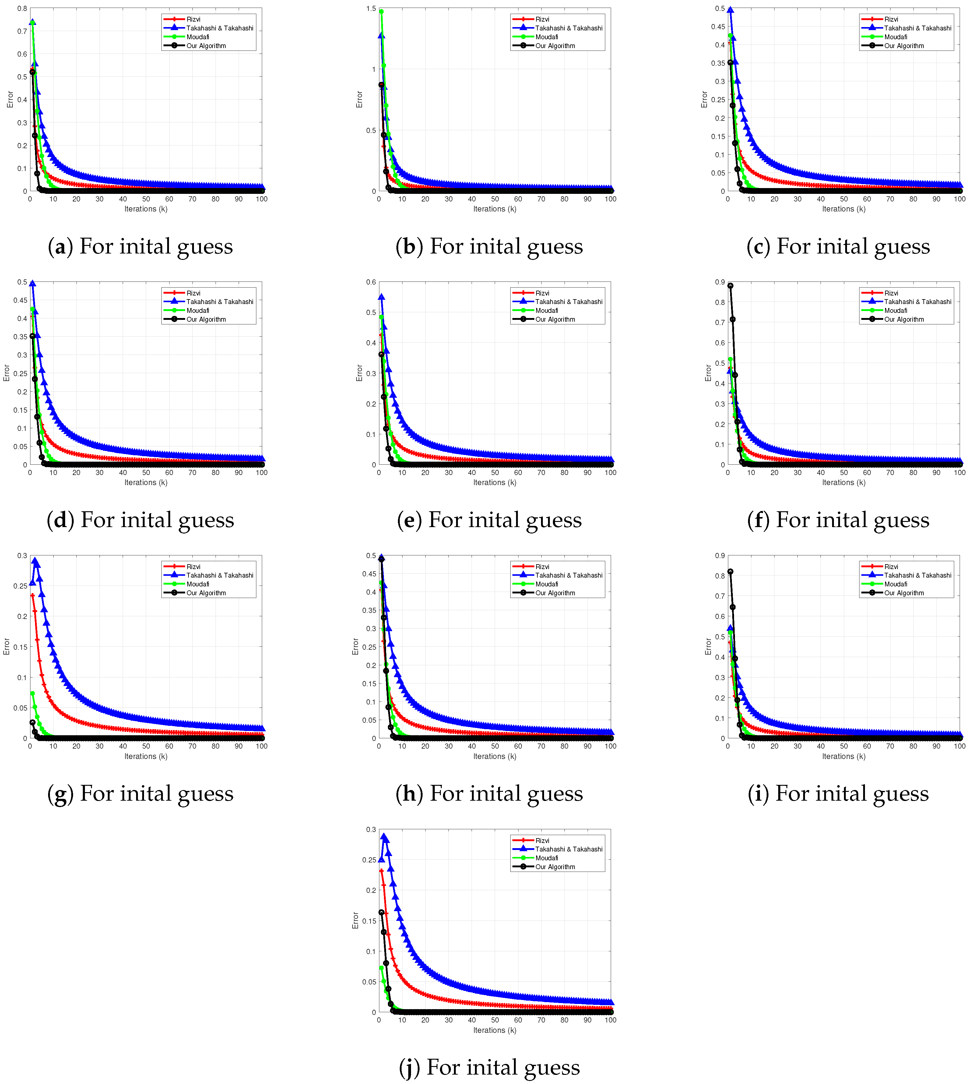
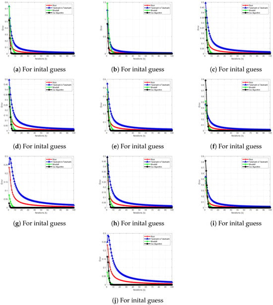
We give our findings in Figure 1.

Figure 1. Convergence of sequence with different initial guesses.

Example 1.

Suppose that ${\mathcal{Z}}_1={\mathcal{Z}}_2=L^2[0,1]$ equipped with the following inner product and norm:

$$⟨u,v⟩={\int }_0^{1}u\left(t\right)v\left(t\right)dt,\mathit{for}\mathit{all}u,v\in L^2[0,1]$$

$$\parallel u\parallel =\sqrt{{\int }_0^1{\left|u\left(t\right)\right|}^{2}dt},\mathit{for}\mathit{all}u\in L^2[0,1].$$

Suppose that $T_1,T_2:L^2[0,1]\to L^2[0,1]$ are given by:

$$T_1\left(u\right)=4u\left(t\right)\mathit{and}{T}_2\left(u\right)=6u\left(t\right).$$

Assume $F,G:L^2[0,1]\times L^2[0,1]\to \mathbb{R}$ are defined by

$$F(u,v)={\int }_0^1(u\left(t\right)-2t)(v\left(t\right)-u\left(t\right))dt,\forall u,v\in L^2[0,1],$$

and

$$G(y,z)={\int }_0^1(y\left(t\right)+4t)(z\left(t\right)-y\left(t\right))dt,\forall y,z\in L^2[0,1].$$

Clearly, F and G satisfy Assumption 1. Define $A,B:L^2[0,1]\to L^2[0,1]$ as follows:

$$B\left(u\right)=-{\displaystyle \frac{9}{4}}u,$$

and

$$A\left(u\right)=-2u.$$

Suppose $\varphi ,\phi :L^2[0,1]\to L^2[0,1]$ are given by

$$\varphi \left(u\right)=2u\mathit{and}\phi \left(u\right)=3u,\forall u\in L^2[0,1].$$

Note that ϕ and φ are the 2 and 3-inverse strongly monotone respectively, and $T_1,T_2$ are maximal monotone mappings.

If, $S\left(u\right)=T\left(u\right)=u$ and

$${\mathcal{J}}_1=\left\{y\in L^2[0,1]:{\int }_0^{1}y\left(t\right)dt=0\right\},$$

then we have

$$P_{{\mathcal{J}}_1}\left(y\right)=y-{\int }_0^{1}y\left(s\right)ds,y\in L^2[0,1].$$

We set $\mathsf{\Phi }\left(u\right)={\displaystyle \frac{u}{2}}$${\alpha }_k={\displaystyle \frac{1}{k+1}}$, ${\beta }_k={\displaystyle \frac{1}{k+2}}$, ${\delta }_k={\displaystyle \frac{k^2+k-1}{k^2+3k+2}}$, $\gamma =0.6$, $z=0.6$, $r_k=0.2$, and $k=100$. The numerical results are presented in Figure 1, where the error decreases toward zero as the number of iterations increases for all considered initial guesses. For comparison, we take different initial guesses given below:

• Initial Guesses:

  (a) 

  $x_0\left(t\right)=1,x_1\left(t\right)=0.8$

  (b) 

  $x_0\left(t\right)=2,x_1\left(t\right)=-1$

  (c) 

  $x_0\left(t\right)=\sin \left(\pi t\right),x_1\left(t\right)=\sin \left(2\pi t\right)$

  (d) 

  $x_0\left(t\right)=t,x_1\left(t\right)=t^2$

  (e) 

  $x_0\left(t\right)=e^{-t},x_1\left(t\right)=e^{-2t}$

  (f) 

  $x_0\left(t\right)=\sin \left(\pi t\right)+t,x_1\left(t\right)=e^{-t}-t$

  (g) 

  $x_0\left(t\right)=\sin \left(5\pi t\right),x_1\left(t\right)=\cos \left(3\pi t\right)$

  (h) 

  $x_0\left(t\right)=0.1,x_1\left(t\right)=0.05$

  (i) 

  $rand{x}_0\left(t\right),x_1\left(t\right)\in (0,1)$, where $rand$ operator picks the random values,

  (j) 

  $x_0\left(t\right)=\left\{\begin{array}{cc}1,\hfill & t<0.5\hfill \\ 0,\hfill & t\ge 0.5\hfill \end{array}\right.,x_1\left(t\right)=\left\{\begin{array}{cc}0,\hfill & t<0.5\hfill \\ 1,\hfill & t\ge 0.5\hfill \end{array}\right.$

From Figure 1, we observe that the error decreases toward zero for all considered initial guesses. The proposed Algorithm 6 and the comparison algorithms exhibit the expected convergence behavior in the numerical experiment with Algorithm 3 [30], Algorithm 4 [31] and Algorithm 5 [35], hence, our proposed Algorithm 6 performs well under different choices of initial guesses.

5. Conclusions

This study introduced an inertial self-adaptive viscosity iterative scheme to find a common solution for the split mixed equilibrium problem, split variational inclusion problem and common fixed point problem of nonexpansive maps. The major strength of this approach is that it is self-adaptive in terms of step size without necessarily knowing the operator norm, hence it is more realistic and simpler than many other approaches in the current literature. In addition, we proved that our proposed algorithm guarantees the convergence of the generated sequence to a common solution of the problems under consideration. Moreover, we proved that the introduced framework is more general than others and as a result, several significant problems including split minimization problems, split common null point problems and split feasibility problems can be derived as special cases. The usefulness and efficiency of the introduced algorithm are illustrated by an example and graphical results.

References

1. Bauschke, H.H.; Borwein, J.M. On projection algorithms for solving convex feasibility problems. SIAM Rev. 1996, 38, 367–426. [Google Scholar] [CrossRef] [Scilit]
2. Chen, P.; Huang, J.; Zhang, X. A primal–dual fixed point algorithm for convex separable minimization with applications to image restoration. Inverse Probl. 2013, 29, 025011. [Google Scholar] [CrossRef] [Scilit]
3. Goebel, K.; Reich, S. Uniform Convexity, Hyperbolic Geometry, and Non-Expansive Mappings; Marcel Dekker: New York, NY, USA, 1984. [Google Scholar]
4. Reich, S.; Shoikhet, D. Nonlinear Semigroups, Fixed Points, and Geometry of Domains in Banach Spaces; Imperial College Press: London, UK, 2005. [Google Scholar]
5. Deutsch, F. Best Approximation in Inner Product Spaces; Springer: Berlin, Germany, 2001. [Google Scholar]
6. Barbagallo, A. Existence and regularity of solutions to nonlinear degenerate evolutionary variational inequalities with applications to dynamic network equilibrium problems. Appl. Math. Comput. 2009, 208, 1–13. [Google Scholar] [CrossRef] [Scilit]
7. Dafermos, S.; Nagurney, A. A network formulation of market equilibrium problems and variational inequalities. Oper. Res. Lett. 1984, 3, 247–250. [Google Scholar] [CrossRef] [Scilit]
8. He, R. Coincidence theorem and existence theorems of solutions for a system of Ky Fan type minimax inequalities in FC-spaces. Adv. Fixed Point Theory 2012, 2, 47–57. [Google Scholar]
9. Qin, X.; Cho, S.Y.; Kang, S.M. Strong convergence of shrinking projection methods for quasi-ϕ-nonexpansive mappings and equilibrium problems. J. Comput. Appl. Math. 2010, 234, 750–760. [Google Scholar] [CrossRef] [Scilit]
10. Censor, Y.; Elfving, T. A multiprojection algorithm using Bregman projections in a product space. Numer. Algorithms 1994, 8, 221–239. [Google Scholar] [CrossRef] [Scilit]
11. Byrne, C. Iterative oblique projection onto convex sets and the split feasibility problem. Inverse Probl. 2002, 18, 441. [Google Scholar] [CrossRef] [Scilit]
12. Byrne, C. A unified treatment of some iterative algorithms in signal processing and image reconstruction. Inverse Probl. 2003, 20, 103. [Google Scholar] [CrossRef] [Scilit]
13. Censor, Y.; Bortfeld, T.; Martin, B.; Trofimov, A. A unified approach for inversion problems in intensity-modulated radiation therapy. Phys. Med. Biol. 2006, 51, 2353. [Google Scholar] [CrossRef] [Scilit] [PubMed]
14. Combettes, P. The convex feasibility problem in image recovery. Adv. Imaging Electron Phys. 1996, 95, 155–270. [Google Scholar] [CrossRef] [Scilit]
15. Xu, H.K. Iterative methods for the split feasibility problem in infinite-dimensional Hilbert spaces. Inverse Probl. 2010, 26, 105018. [Google Scholar] [CrossRef] [Scilit]
16. Yang, Q. The relaxed CQ algorithm solving the split feasibility problem. Inverse Probl. 2004, 20, 1261. [Google Scholar] [CrossRef] [Scilit]
17. Moudafi, A. Split monotone variational inclusions. J. Optim. Theory Appl. 2011, 150, 275–283. [Google Scholar] [CrossRef] [Scilit]
18. Censor, Y.; Gibali, A.; Reich, S. Algorithms for the split variational inequality problem. Numer. Algorithms 2012, 59, 301–323. [Google Scholar] [CrossRef] [Scilit]
19. Tang, Y. Convergence analysis of a new iterative algorithm for solving split variational inclusion problems. J. Ind. Manag. Optim. 2020, 16, 945. [Google Scholar] [CrossRef] [Scilit]
20. Halpern, B. Fixed points of nonexpanding maps. Bull. Am. Math. Soc. 1967, 73, 957–961. [Google Scholar] [CrossRef] [Scilit]
21. Iiduka, H. Fixed point optimization algorithm and its application to network bandwidth allocation. J. Comput. Appl. Math. 2012, 236, 1733–1742. [Google Scholar] [CrossRef] [Scilit]
22. Kazmi, K.R.; Rizvi, S.H. An iterative method for split variational inclusion problem and fixed point problem for a nonexpansive mapping. Optim. Lett. 2014, 8, 1113–1124. [Google Scholar] [CrossRef] [Scilit]
23. Luo, C.; Ji, H.; Li, Y. Utility-based multi-service bandwidth allocation in the 4G heterogeneous wireless access networks. In Proceedings of the IEEE Wireless Communications and Networking Conference, Budapest, Hungary, 5–8 April 2009; pp. 1–5. [Google Scholar]
24. Moudafi, A. Viscosity approximation methods for fixed-point problems. J. Math. Anal. Appl. 2000, 241, 46–55. [Google Scholar] [CrossRef] [Scilit]
25. Abbas, M.; Asghar, M.W.; De la Sen, M. Approximation of the solution of delay fractional differential equation using AA-iterative scheme. Mathematics 2022, 10, 273. [Google Scholar] [CrossRef] [Scilit]
26. Asghar, M.W.; Abbas, M.; Eyni, D.C.; Omaba, M.E. Iterative approximation of fixed points of generalized αm-nonexpansive mappings in modular spaces. AIMS Math. 2023, 8, 26922–26944. [Google Scholar] [CrossRef] [Scilit]
27. Beg, I.; Abbas, M.; Asghar, M.W. Convergence of AA-iterative algorithm for generalized α-nonexpansive mappings with an application. Mathematics 2022, 10, 4375. [Google Scholar] [CrossRef] [Scilit]
28. Suanoom, C.; Gebrie, A.G.; Grace, T. The convergence of AA-iterative algorithm for generalized AK-α-nonexpansive mappings in Banach spaces. Sci. Technol. Asia 2023, 10, 82–90. [Google Scholar]
29. Byrne, C.; Censor, Y.; Gibali, A.; Reich, S. The split common null point problem. J. Nonlinear Convex Anal. 2012, 13, 759–775. [Google Scholar]
30. Moudafi, A. Weak convergence theorems for nonexpansive mappings and equilibrium problems. J. Nonlinear Convex Anal. 2008, 9, 37. [Google Scholar]
31. Takahashi, S.; Takahashi, W. Strong convergence theorem for a generalized equilibrium problem and a nonexpansive mapping in a Hilbert space. Nonlinear Anal. Theory Methods Appl. 2008, 69, 1025–1033. [Google Scholar] [CrossRef] [Scilit]
32. Tada, A.; Takahashi, W. Weak and strong convergence theorems for a nonexpansive mapping and an equilibrium problem. J. Optim. Theory Appl. 2007, 133, 359–370. [Google Scholar] [CrossRef] [Scilit]
33. Kazmi, K.R.; Rizvi, S.H. A hybrid extragradient method for approximating the common solutions of a variational inequality, a system of variational inequalities, a mixed equilibrium problem and a fixed point problem. Appl. Math. Comput. 2012, 218, 5439–5452. [Google Scholar] [CrossRef] [Scilit]
34. Takahashi, S.; Takahashi, W. Viscosity approximation methods for equilibrium problems and fixed point problems in Hilbert spaces. J. Math. Anal. Appl. 2007, 331, 506–515. [Google Scholar] [CrossRef] [Scilit]
35. Rizvi, S.H. A Mann-Halpern algorithm for solving split null point, split mixed equilibrium and fixed point problems for a nonexpansive mapping. Numer. Algorithms 2026, 1–27. [Google Scholar] [CrossRef] [Scilit]
36. Alakoya, T.O.; Owolabi, A.; Mewomo, O.T. An inertial algorithm with a self-adaptive step size for a split equilibrium problem and a fixed point problem of an infinite family of strict pseudo-contractions. J. Nonlinear Var. Anal. 2021, 5, 803–829. [Google Scholar] [CrossRef] [Scilit]
37. Asghar, M.W.; Abbas, M. A self-adaptive viscosity algorithm for split fixed point problems and variational inequality problems in Banach spaces. J. Nonlinear Convex Anal. 2023, 24, 341–361. [Google Scholar]
38. Izuchukwu, C.; Ogwo, G.; Mewomo, O. An inertial method for solving generalized split feasibility problems over the solution set of monotone variational inclusions. Optimization 2022, 71, 583–611. [Google Scholar] [CrossRef] [Scilit]
39. Shehu, Y.; Iyiola, O.S.; Ogbuisi, F.U. Iterative method with inertial terms for nonexpansive mappings: Applications to compressed sensing. Numer. Algorithms 2020, 83, 1321–1347. [Google Scholar] [CrossRef] [Scilit]
40. Shehu, Y.; Iyiola, O.S.; Thong, D.V.; Cam Van, T.C. An inertial subgradient extragradient algorithm extended to pseudomonotone equilibrium problems. Math. Methods Oper. Res. 2021, 93, 213–242. [Google Scholar] [CrossRef] [Scilit]
41. Zhao, J.; Liang, Y.; Liu, Y.; Cho, Y.J. Split equilibrium, variational inequality and fixed point problems for multi-valued mappings in Hilbert spaces. Appl. Math. Comput. 2018, 17, 271–283. [Google Scholar]
42. Chuang, C.S. Strong convergence theorems for the split variational inclusion problem in Hilbert spaces. Fixed Point Theory Appl. 2013, 2013, 350. [Google Scholar] [CrossRef] [Scilit][Green Version]
43. Osilike, M.O.; Igbokwe, D.I. Weak and strong convergence theorems for fixed points of pseudocontractions and solutions of monotone type operator equations. Comput. Math. Appl. 2000, 40, 559–567. [Google Scholar] [CrossRef] [Scilit]
44. Maingé, P.E. Approximation methods for common fixed points of nonexpansive mappings in Hilbert spaces. J. Math. Anal. Appl. 2007, 325, 469–479. [Google Scholar] [CrossRef] [Scilit]
45. Saejung, S.; Yotkaew, P. Approximation of zeros of inverse strongly monotone operators in Banach spaces. Nonlinear Anal. Theory Methods Appl. 2012, 75, 742–750. [Google Scholar] [CrossRef] [Scilit]
46. Aubin, J.P. Optima and Equilibria: An Introduction to Nonlinear Analysis; Springer: Berlin, Germany, 2002. [Google Scholar]
47. Moudafi, A.; Thakur, B.S. Solving proximal split feasibility problems without prior knowledge of operator norms. Optim. Lett. 2014, 8, 2099–2110. [Google Scholar] [CrossRef] [Scilit]
48. Abbas, M.; AlShahrani, M.; Ansari, Q.H.; Iyiola, O.S.; Shehu, Y. Iterative methods for solving proximal split minimization problems. Numer. Algorithms 2018, 78, 193–215. [Google Scholar] [CrossRef] [Scilit]
Disclaimer/Publisher’s Note: The statements, opinions and data contained in all publications are solely those of the individual author(s) and contributor(s) and not of MDPI and/or the editor(s). MDPI and/or the editor(s) disclaim responsibility for any injury to people or property resulting from any ideas, methods, instructions or products referred to in the content.
Article Metrics
Citations
Article Access Statistics
Multiple requests from the same IP address are counted as one view.