


Abstract
Symmetry in nuclear and electromagnetic properties of matter and antimatter seems to imply similar structures and evolution for matter and antimatter celestial objects. However, antimatter domains originating from strongly inhomogeneous baryosynthesis evolve within a baryon-asymmetric universe under the asymmetric conditions of the surrounding baryonic matter. This asymmetry leads to annihilation at their borders and localized chemical evolution within the domains. The specifics of this evolution, constrained by the conditions required for the creation and survival of these domains, are the subject of this study. In the model of spontaneous baryosynthesis, the creation of an antibaryon excess may be accompanied by the formation of closed domain walls at their borders; consequently, large domains may remain in baby universes, separated from the observed universe by the dominant domain walls enclosing them. Domains that avoid such separation must be sufficiently large to survive despite ongoing annihilation at their boundaries. Over a large range of antibaryon densities, these surviving domains retain a physical symmetry with matter during the period of big bang nucleosynthesis, leading to the creation of primordial antihelium-4. The successive evolution of these domains proceeds under the competing conditions of diffusion and boundary annihilation. In domains that survive this annihilation, evolution results in the formation of Population III antimatter objects. However, the subsequent chemical composition of antimatter within the domain cannot be enriched by the product of anti-stellar nucleosynthesis. Our analysis proves that primordial macroscopic antimatter can naturally act as a source of antihelium-4, making it possible to detect in the AMS-02 experiment. Nevertheless, the observable properties of such macroscopic antimatter in our galaxy should differ fundamentally from those of observed baryonic objects.
1. Introduction
The observed dominance of matter over antimatter in the present universe constitutes one of the most profound open questions in modern cosmology. Current understanding assumes a global baryon asymmetry, quantified by the baryon-to-photon ratio
which implies the absence of macroscopic antimatter regions in quantities comparable to those of baryonic matter. The origin of this asymmetry is generally attributed to baryogenesis—the physical process that generated the observed baryon excess during the earliest stages of the primordial universe. A viable mechanism of baryogenesis must satisfy the three Sakharov criteria: (i) baryon number violation, (ii) violation of C and symmetry, and (iii) departure from the thermal equilibrium [1]. While the Standard Model of particle physics provides violation, it is insufficient in accounting for the observed magnitude of the asymmetry, necessitating physics beyond the Standard Model [2].
Remarkably, under certain conditions, the local generation of antimatter domains remains theoretically possible. If baryosynthesis were strongly nonhomogeneous—a scenario that can arise, for instance, from spontaneous violation or from the Affleck–Dine mechanism in supersymmetric theories [3]—macroscopic regions with antibaryon excess could have been created alongside the baryonic matter. In such frameworks, the baryon asymmetry is not spatially uniform; instead, the universe may contain isolated domains where antimatter predominates, surrounded by a baryon-dominated medium. Globally, the universe is filled with baryonic matter; however, local regions, or domains, may exist within it where antimatter predominates [4,5].
The laws of strong and electromagnetic interactions are identical for baryons and antibaryons—a direct consequence of symmetry. From this, it follows that the evolution of antimatter can be described analogously to the evolution of matter. Antimatter domains of sufficient size (≳) could survive to the present epoch, with annihilation occurring primarily at the boundaries between matter and antimatter regions. The existence of such domains is subject to observational constraints from big bang nucleosynthesis [6], the cosmic microwave background, and diffuse gamma-ray backgrounds [7].
The AMS-02 experiment, conducted on the International Space Station, enables the detection of antihelium nuclei among the helium nuclei of cosmic rays [8]. The AMS-02 collaboration has tentatively reported the observation of approximately eight to twelve antihelium candidate events—six in the mass range of antihelium-3 and two to four candidates in the mass range of antihelium-4. These candidate events, if confirmed, cannot be readily explained by conventional astrophysical sources and would imply the existence of primordial antimatter objects in our galaxy [9]. Such a detection would immediately reduce the class of inflationary baryosynthesis models to those capable of producing antimatter domains of surviving size. Confirming these results would validate the existence of isolated antimatter domains in the universe, providing a crucial window into the physics of the very early cosmos [10].
2. Antimatter Domain in Baryon Asymmetrical Universe
Antimatter Excess from Nonhomogeneous Baryosynthesis
In standard cosmology, the imbalance between matter and antimatter in the universe is explained by a process called baryosynthesis. If this process is nonhomogeneous, it could lead to creation of regions, or domains, where antimatter predominates [11,12].
The evolutionary dynamics of the antimatter domain over time are primarily determined by its size and chemical composition. In a zeroth-order approximation, we consider a spherical domain to estimate its scale. There are certain observational constraints that will affect this characteristic [13,14,15].
Since the domain consists of antimatter, annihilation occurs at its boundary once it enters the cosmological horizon. This process drives the gradual erosion of the domain over time. Assuming that the domain has survived to the present epoch, it must be sufficiently large, establishing a minimum mass threshold of .
Furthermore, the diffuse gamma-ray background produced by boundary annihilation processes must remain consistent with observational limits [16]. This constraint imposes an upper bound on the domain mass. Accounting for these criteria yields the viable mass range for the domain.
We assume that the domain formed prior to the epoch of big bang nucleosynthesis (BBN). The presence of heavy metallicity within the domain would induce interactions with the surrounding matter, triggering annihilation processes that would yield observable gamma-ray signatures. Consequently, the domain must remain free of heavy elements. This specific chemical composition imposes strict constraint on its density. Specifically, the domain must consist primarily of antihydrogen and antihelium, while completely lacking elements from carbon onward.
The main parameter characterizing the domain density is the baryon-to-photon ratio, which quantifies the abundance of antibaryons relative to photons. This physical quantity determines the resulting mass fractions of chemical elements synthesized with the domain.
To analyze the dependence of these mass fractions on the baryon-to-photon ratio, we employ the AlterBBN code, which is a public C program designed to calculate elemental abundances from big bang nucleosynthesis, using the baryon-to-photon ratio as the primary input parameter.
The mass fraction of 4He increases with the baryon-to-photon ratio , reaching the standard observed value (≈25%) at . Conversely, the production of 4He is almost negligible (less than 1%) at a lower ratio of .
The generation threshold for anticarbon-12 12C was investigated in the density range . At , an uptick in the elemental mass fraction occurs, leading to a rapid onset of secondary production. This obtained threshold serves as a conservative upper bound for the viable domain density range.
Thus, the domain must satisfy two primary physical criteria:
- Adequate antihelium-4 4He abundance to facilitate radiative cooling and subsequent gravitational collapse into Population III antimatter objects;
- Suppression of anticarbon-12 12C production, as the presence of carbon and heavier elements would trigger highly observable, non-standard annihilation signatures.
Based on these numerical findings, the viable density corridor required for the survival of the antimatter domain is bounded by:
Crucially, the upper bound is conservative; in practice, domains with exhibit significantly higher survival probabilities, as elevated interior densities enhance boundary annihilation and accelerate domain erosion. The dependence of the antihelium-4 and anticarbon-12 mass fraction on the baryon-to-photon ratio is illustrated in Figure 1 and in Figure 2, respectively.
Figure 1.
Dependence of the mass fraction of 4He on baryon/photon ratio.
Figure 2.
Dependence of the mass fraction of 12C on baryon/photon ratio.
Based on these numerical findings, the viable density corridor required for the survival of the antimatter domain is bounded by:
The physical scale of the domain is determined jointly by its total mass and interior density. Assuming spherical symmetry, the scaling relation for the domain radius R can be expressed as:
Consequently, at any given cosmological epoch, the domain radius is strictly bounded by the allowed intervals of its primary parameters, namely mass and density.
The physical size of the domain dictates both its internal chemical evolution and boundary microphysics. Once the cosmological Hubble horizon expands to exceed the spatial scale of the domain, macroscopic baryon–antibaryon annihilation is initiated at the boundary interface. Tracking the interplay between these two length scales across different cosmic epochs is therefore essential.
To establish a precise chronological timeline, we derive a numerical estimate for the exact moment of horizon entry. We assume that this entry occurs during the radiation-dominated era (characterized by ultra-relativistic matter dominance), where the governing cosmological scaling laws yields:
Solving this inequality provides the characteristic timescales at which the domain enters the cosmological horizon:
Evaluating this expression over the viable mass and density ranges yields the following entry range:
- s;
- s.
Crucially, these computed boundaries fall squarely within the radiation-dominated epoch of the early universe, validating our initial cosmological assumptions.
3. Processes at the Border
Following the aforementioned assumptions, the domain enters the horizon during the radiation-dominated era. Subsequently, baryon–antibaryon annihilation is initiated at the domain boundary. In this framework, we consider proton–antiproton annihilation.
The primary stable products of this annihilation process consist of high-energy photons from the decay of neutral pions and electron–positron pairs derived from the decay chain of charged pions [17,18]. Each of these specific production channels is reviewed below.
3.1. Neutral Pion Decay
The decay of a neutral pion yields two high-energy photons. In the pion rest frame, these photons carry a mean energy of . The spectral distribution of the resulting high-energy photons is distributed uniformly [19]. Given that an average of one to three neutral pions are produced per annihilation event, the mean photon multiplicity generated via this channel is [18].
3.2. Charged Pion Decay
Concurrently, proton–antiproton annihilation pathways frequently result in the production of charged pions.
These charged pions subsequently decay into muons and their corresponding (anti)neutrinos. For the purposes of tracking domain ionization, the primary channel of interest is the subsequent three-body decay of the muon into an electron or positron.
In the rest frame of the parent pion, the generated muon carries a discrete energy of . The energy distribution of leptons produced via negative muon decay is governed by the Michel spectrum [20]. Consequently, the laboratory-frame energy of the emerging electron is bounded within the kinematic range .
3.3. Antimatter Domain in the Model of Spontaneous Baryosynthesis
A mechanism for the generation of primordial antimatter domains arises from the field dynamics of a pseudo-Nambu–Goldstone boson (PNGB) within a framework of spontaneous baryogenesis. Post-phase transition, the field theory is governed by the Lagrangian density in Equation (12). Within this specific framework, it has been shown in [3,21,22,23] that the dynamical evolution of the PNGB field determines the sign of the generated asymmetry: a trajectory rolling within the formal angular interval toward the potential minimum generates a baryon excess, whereas a trajectory rolling within the opposite phase boundary produces a net antibaryon excess. Exploiting the discrete periodic symmetry of the potential , any field trajectory rolling within the alternative angular transition bound similarly yields an antibaryon excess, ensuring complete mathematical coverage of the phase space:
During inflation, super-horizon quantum fluctuations in the PNGB field can drive spatial regions across the critical phase threshold , culminating in the formation of closed domain walls. In this topological configuration, the spatial interior of the closed wall encloses a local antibaryon excess, while the surrounding background medium remains baryon-dominated. The spatial scale of these non-vanishing fluctuations is determined by the inflationary Hubble parameter, . Consequently, a quantum fluctuation nucleated at time t expands to a physical scale by the end of cosmological inflation, governed by:
Following the cessation of inflation, these spatial profiles undergo power-law stretching driven by subsequent cosmic expansion. The onset of coherent classical motion of the PNGB field, which triggers the physical realization of the closed domain walls, begins when the background Hubble parameter H decays to the scale of the effective PNGB mass, namely .
The mass of this scalar field imposes a strict lower bound on the survival scale of the antimatter domain, since fluctuations with wavelengths smaller than the horizon at the onset of classical motion are unable to survive. Consequently, the minimum domain radius is uniquely determined by the horizon scale at this triggering epoch:
Conversely, the upper bound on the spatial extent of the domain size is constrained by the surface tension of the wall. A closed domain wall that has a constant surface energy density can achieve a local energy density dominance within its volume before entering the global cosmological horizon, provided that its initial radius is sufficiently large. Following [24,25], the characteristic cosmological timescale for the wall to achieve dominance that potentially collapses into an isolated baby universe is expressed by:
where denotes the surface energy density. For the PNGB profile under consideration, this surface tension is derived analytically from the model parameters as , yielding:
Compiling these microphysical boundaries yields the final allowed window for the primordial antimatter domain radius :
Using these spatial constraints, we map the geometric boundaries to an allowed mass threshold for the surviving antimatter domains. Let denote the baseline baryon mass and represent the physical baryon number density at the exact instance of horizon crossing. The total net antimatter mass M enclosed within the domain is strictly bounded by the inequality:
4. Processes Inside the Domain
The high-energy products generated via boundary annihilation penetrate into the deep interior of the antimatter domain [26,27,28]. This continuous particle influx triggers an array of secondary physical processes within the bulk volume.
4.1. Pair Production
As the high-energy photons generated during proton–antiproton annihilation penetrate the domain, they interact with the ambient thermal radiation field. The production of electron–positron pairs via photon scattering becomes kinematically allowed. For this interaction to occur, the thermal photon energy must satisfy the threshold condition .
The spectral distribution of these thermal photons is governed by the Planck blackbody spectrum, which guarantee a non-zero number density of energetic photons. The specific fraction of photons fulfilling the requirement within the Planck distribution can be calculated analytically as follows:
According to that, the concentration of high-energy photons becomes negligible (less than 1%) at temperatures below K. Consequently, only during the time period s is the formation of positron–electron pairs inside the domain possible.
The interaction of two photons is described by the Breit–Wheeler formula for high energies. Note that the energy of the thermal photon is significantly lower than that of the annihilation photon. In this case, an energy asymmetry is observed, and the formula describing the reaction cross-section will take the following form [29]:
where
- ;
- .
4.2. Compton Scattering
In addition to the formation of electron–positron pairs inside the domain, Compton scattering of a photon on a positron is also possible. This process will become dominant at K.
The change in energy after a single Compton scattering process is described by the following equation:
Assuming that the scattering is isotropic, the relative energy loss will be:
where .
For high-energy annihilation photons (∼10–100 MeV), the scattering occurs strictly in the Klein–Nishina regime (), where Equation (22) correctly ensures that the fractional energy loss remains physically bounded .
The classical expression incorporating thermal corrections is given by:
The soft-photon approximation only becomes applicable at later stages of multiple scattering, once the photons have successfully cooled down to the non-relativistic Thomson regime (). In the sub-MeV regime, if the photon energy still dominates the ambient plasma temperature (), the thermal motion term can be neglected, yielding , which remains perfectly bounded and physically plausible since . Note that a photon does not lose all its energy in a single scattering event. It is important to estimate how many scattering events are required to reduce the photon energy to 1 MeV.
The evolution of the photon distribution under multiple scattering is described by the Kompaneets equation [30]. In our case, the dominant process will be photon cooling (induced scattering might be negligible). The Kompaneets equation simplifies to the following form:
where
- n—the number of photons in a state with dimensionless energy x;
- y—Compton parameter.
From the solution of this equation, it follows that the energy changes will have exponential character:
The Compton parameter correlates with the number of scatterings in the following way:
From which we get:
For our temperature range, the number of necessary processes will be
Let us now estimate the interaction cross-section for this reaction. According to the Klein–Nishina formula:
where
- —Thomson scattering cross-section;
- —correction factor for relativistic effects.
As the photon energy decreases, the cross-section value will approach the Thomson scattering cross-section. Taking into account the numerical solutions of the Kompaneets equation, we obtain
According to the estimated values, we will get the effective parameter that describes multiple scattering.
4.3. Temperature Dependencies
To summarize, since the temperature decreases, it is necessary to consider different scenarios.
During the time period corresponding to the temperature K, the leading process affecting the mean free path of an annihilation photon can be considered to be pair production, due to the high concentration of thermal photons in the radiation-dominated epoch. The total interaction cross-section for an annihilation photon at this temperature is:
Starting from the moment when the domain temperature reaches K, the formation of positron–electron pairs becomes unlikely, even considering the high-energy tail of the Planck distribution. In this case, the leading process affecting the mean free path of an annihilation photon should be considered to be Compton scattering on positrons. The interaction cross-section for an annihilation photon in this case is:
5. Diffusion
5.1. Diffusion Mechanism in Radiation-Dominated Era (RD)
We model the antimatter domain as a sphere of comoving radius , whose physical radius scales with the expansion of the universe following . Under spherical symmetry, all physical quantities depend only on the comoving radius r and time t. The diffusion operator is reduced to the radial component of the Laplacian
The transport of baryons and antibaryons toward the domain boundaries is not governed by annihilation but by elastic scattering processes:
- Proton–electron Coulomb scattering: This is the most efficient mechanism for charged baryons. Protons interact directly with electrons via the Coulomb force. Concurrently, electrons are coupled to the photon bath through Thomson scattering.The transport of protons is limited by the electron mobility due to the requirement of maintaining local charge neutrality, making electron–photon coupling the main constraint on baryon diffusion.
- Indirect proton–photon scattering: Protons do not scatter directly off photons with a significant cross-section. Instead, they are coupled to the radiation field via mediated scattering with electrons.
- Direct proton–photon scattering: The cross-section for this mechanism is extremely small () and negligible for diffusion in the early universe.
In a medium where particles undergo frequent elastic collisions, the diffusion coefficient relates the particle flux to the density gradient. From kinetic theory [31],
where is the mean free path and is the thermal velocity. In the radiation-dominated era, this equation describes the baryon diffusion coefficient, where corresponds to the thermal velocity of baryons, and is governed by the dominant scattering mechanisms. The mean free path for the scattering of electrons is defined by [32]
where is the electron number density and is the elastic cross-section.
During the radiation-dominated era, the scale factor evolves with time as . Also, the number density evolution of baryons follows the law
where the present-day scale factor is normalized to 1. Using the time dependence of the scale factor , the evolution of the number density can be expressed as a function of time:
Assuming that the elastic cross-section remains constant over the relevant temperature range, the electron number density evolves identically to the baryon number density . Consequently, the mean free path (38) can be expressed as a function of time:
The consequence is that the diffusion becomes more efficient as the universe expands and the plasma becomes more transparent.
The plasma temperature scales as . The diffusing baryons are non-relativistic and in thermal equilibrium with the plasma, so their thermal velocity evolves as
Substituting the time dependence of the mean free path and the thermal velocity into Equation (37), the diffusion coefficient in the radiation-dominated era scales as
5.2. Annihilation Products and Radiation Pressure Feedback
The diffusion process is not static; rather, it is modulated by active feedback from the annihilation products themselves. When antibaryons annihilate at the domain boundaries, they release energetic particles that alter the local properties of the plasma.
Proton-antiproton annihilation primarily produces pions:
Also, muons decay as
The final stable products consist of high-energy photons originating from decay, relativistic electron–positron pairs produced by muon , and neutrinos . Each annihilation event is characterized by a mean particle multiplicity, denoted as , representing the average number of electrons and positrons produced, with a similar number of photons. For the case of proton–antiproton annihilation, the average photon energy is approximately 180 MeV, while electrons and positrons carry an estimated average energy of approximately 90 MeV. The energy partition is distributed as follows: for neutrinos, for photons and for electron–positron pairs.
At the domain boundary, the dynamical equilibrium described by a Stefan-type boundary condition balances the diffusive flux of antibaryons toward the boundary with their annihilation rate. For a spherical domain with a radius , this balance is expressed as:
where is the diffusion coefficient, is the radial gradient of the antibaryon density at the boundary, and is an efficiency factor accounting for the fraction of encounters that result in annihilation. Furthermore, and are the baryon and antibaryon densities evaluated at the boundary and is the effective thickness of the annihilation layer.
In the case of a small, spherically symmetric domain, the antibaryon number density in the linear approximation scales according to the following profile:
Consequently, the resulting boundary flux depends on the initial antiproton density and the dynamic spatial size of the domain:
Using the previously established temperature dependencies for the domain size , the background number density , and the diffusion coefficient , we obtain the final scaling law for the flux as a function of temperature:
Energetic electron–positron pairs deposit their energy into the surrounding plasma through Coulomb interactions, keeping it ionized and generating a local pressure excess.
where is a radiative relaxation time, is the energy released per annihilation and is the local annihilation rate per unit volume. The pressure gradient acts as a drift force, accelerating fluid elements toward the annihilation boundary. The drift force is incorporated as the second term in the generalized Fick’s law
The validity of this ideal-fluid approximation in the thin layer rests on the clear separation of length scales at the domain boundary. The annihilation interface has a thickness , where is the annihilation timescale, while the reheated zone extends over , the stopping length of annihilation-produced electrons. The hierarchy is established as , with , so the boundary layer is compared to the domain radius . Since the mean free path satisfies , the local thermodynamic equilibrium is established . The bulk of the domain therefore evolves as an ideal fluid, and the diffusive transport is perfectly described by the Fickian form of Equation (49), where the drift term accounts for the annihilation pressure gradient without the violation of fluid approximation.
5.3. Effective Diffusion Coefficient and Thin-Boundary Condition
At the domain boundary, the density and pressure gradients are steep but confined to a narrow layer of thickness . Under the thin-boundary approximation, these radial gradients can be approximated as
where the negative signs reflect that both the antibaryons density and the annihilation pressure decreases sharply as one moves outward across the boundary layer.
Substituting the thin-boundary approximation (50) into the generalized flux Equation (49) allows the flux to be cast in the form of a standard Fick’s law governed by an effective diffusion coefficient
where
The thin-boundary approximation is justified if the heating zone is significantlywider than the annihilation layer itself. The characteristic width of this reheated zone is denoted by L, which represents the distance over which annihilation-produced electrons deposit their thermal energy [33]:
where . For redshifts between and , the reheating zone is estimated to be approximately and , respectively. The validity of this approach relies on the strict length-scale hierarchy , where A is the thickness of the annihilation zone, D is the width of the depletion zone and L is the span of the reheated zone.
Table 1.
Cosmological parameters at different redshifts.
Figure 3.
Reheated zone as a function of redshift.
5.4. Diffusion Mechanisms Between Radiation-Dominated Era and Matter-Dominated Era
The transition from the radiation-dominated (RD) to matter-dominated (MD) era is marked by the growing dominance of non-relativistic matter over radiation. During the interval between matter–radiation equality and hydrogen recombination , the primordial plasma remains fully ionized, and the diffusion of baryons and antibaryons continues to be governed by radiative friction mechanisms, even though the expansion law of the universe has changed. The diffusion coefficient in this regime, denoted as , can be derived from kinetic theory (37):
where is the mean free path and is the thermal speed of the diffusing particles, defined as . The mean free path for Coulomb scattering is inversely proportional to the electron number density:
In an expanding universe, . Hence,
Using the matter-dominated era scaling law , we obtain
The thermal velocity of electrons scales as . During the adiabatic expansion of the matter-dominated era, the temperature of coupled plasma is expressed as :
However, in the limit of tight coupling, the effective momentum exchange is dominated by Compton scattering, and the effective diffusion coefficient is set by the balance between pressure force and radiation drag (Appendix A):
Consequently, diffusion becomes significantly more efficient during the pre-recombination matter-dominated era. This accelerated transport enhances the flux of antibaryons toward the domain boundary.
5.5. Diffusion Mechanism in Matter-Dominated Era (MD)
The transition to the matter-dominated era (MD) is marked by the dominance of non-relativistic matter. At the epoch of recombination occurring at a time , redshift and temperature when electrons and protons combine to form neutral hydrogen atoms [33]. At this point, the underlying mechanism of diffusion changes completely. The kinetic theory for neutral gas gives the diffusion coefficient expressed as
where is the collision mean free path and is the thermal velocity.
The collision mean free path is expressed as
where is the number density of baryons–antibaryons and is the atomic collision cross-section, which is approximately constant for neutral hydrogen. The number density of baryons scales with the expansion of the universe according to
Assuming that varies slowly with the temperature, the mean free path scales as
After recombination, the neutral matter is no longer coupled to the radiation field and cools adiabatically. For a monoatomic gas expanding adiabatically, the material temperature relates to the volume V and the scale factor as:
where is the adiabatic index. This simplifies directly to:
Substituting the scaling laws for the mean free path (65) and the thermal velocity (68) into the atomic diffusion coefficient (61) yields:
In the matter-dominated era, the scale factor evolves as . Consequently, the atomic diffusion coefficient evolves over time according to:
In theory, the diffusion coefficient described by Equation (70) is correct for the bulk background but cannot govern the erosion of the antimatter domain. The annihilation at the boundary produces energetic electron–positron pairs that deposit their energy locally, maintaining a thin, fully ionized plasmalayer at the boundary interface. Consequently charged antibaryons like remain coupled to the radiation field via electromagnetic interactions. The transport of antibaryons to the annihilation boundary is controlled by plasma diffusion (60), rather than by atomic diffusion (70). For the erosion of domain, the relevant diffusion coefficient remains the plasma diffusion coefficient (60) derived in Appendix A.
The annihilation pressure gradient, generated by local energy deposition, induces an additional drift. The generalized Fick’s law should employ the plasma diffusion coefficient for both terms:
where is the annihilation pressure. In the matter-dominated era, this pressure scales as:
where is a characteristic collision time for energy confinement. Applying the thin boundary approximation of (50) yields the effective diffusion coefficient:
The persistence of plasma diffusion at the domain boundaries ensures that erosion continues efficiently long after recombination.
The continuity of plasma diffusion mechanisms in the matter-dominated era across the recombination epoch significantly simplifies the modeling of domain evolution and enables a unified treatment from the radiation-dominated era to the present day (Table 2).
Table 2.
Scaling of diffusion coefficients in different regimes.
6. Ionization
The next process that must be taken into account to describe the evolution of the antimatter domain over time is the ionization of antimatter, which will be caused by the products of proton–antiproton annihilation at the boundary. If the ionization of matter is sufficiently high, it must be taken into consideration in describing the evolution of the domain.
In contrast to the planar model [33], where ionizing radiation propagates along an infinite boundary, for a spherical anti-domain of radius R, the radiation from annihilation on the surface diverges radially and is absorbed in a thin near-surface layer. This leads to a significant inhomogeneity of ionization.
It should be noted that two regions must be considered:
- The boundary region of the domain at the horizon.In this case, ionization will occur due to high-energy electrons produced as a result of annihilation. The size of this region is determined by the mean free path of the electrons.
- The inner region of the domain.While describing the inner volume of the domain, it is also necessary to take into account secondary processes. According to [33], the ionization mechanism in this case will be as follows:
- Annihilation of at the surface of the domain:
- Decay of charged pions producing relativistic electrons/positrons:The average energy of the electron: . The average number of electrons per annihilation event: .
- Inverse Compton scattering of relativistic electrons on CMB photons:As a result, CMB photons gain energy and are converted into UV photons (their energy is of the order of 10–).
- Photoionization of atomic antihydrogen by UV photons:
Direct ionization by photons produced in the decay of neutral pions can be neglected due to the smallness of the photoionization cross-section.
To describe processes of ionization, the penetration depth of electrons and UV photons should be estimated.
The energy loss of relativistic electrons occurs via Compton scattering on CMB photons. In this case, the electron mean free path might be estimated using the following formula:
where for initially relativistic electrons and
is the loss coefficient.
UV photons are absorbed by atomic hydrogen with a photoionization cross-section .
The absorption length of an ultraviolet photon can be calculated using the standard formula:
where is the concentration of antihydrogen atoms inside the domain.
Since the domain that we are considering has a finite radius, it is necessary to move from the existing planar geometry models [33] to a spherical one. We assume that, as a result of annihilation over the entire surface of the domain, electrons are produced and then penetrate into the interior of the domain. In this approximation, we also assume that the electrons move strictly radially.
We assume that, after a single process of annihilation, electrons are produced [34]. Then, the total number of electrons emitted by the surface per unit time is
These electrons move radially inside the domain, losing energy over a length . In the stationary regime, the electron flux satisfies the continuity equation. Let us write it considering the spherical geometry:
The right term of the equation takes into account the loss of electrons due to their energy decreasing below the threshold for the production of UV photons. This equation is solved based on the boundary condition , which defines the electron flux at the boundary. After substitution, we obtain:
The factor reflects the geometry considered in the problem, while the exponential describes the change in the number of electrons capable of producing UV photons that lead to ionization.
Let each electron produce UV photons at a rate . Then, the volumetric production rate of UV photons is:
The flux density of UV photons at a point r is found from the transport equation:
In the limit of strong absorption (), the last factor tends to 1, as a result of which the final formula takes the form:
Taking into account that about 0.1 of the electron energy is transferred to the UV photon energy, the formula takes the form:
The last factor, in this case, arises from taking into account the absorption of UV photons in the antimatter layer within the domain.
One of the most important characteristics that must be taken into account when describing the evolution of the domain is the degree of ionization of antimatter both at the boundary and within the region. Let us consider a method for estimating this quantity.
6.1. The Boundary Region
As mentioned earlier, ionization in the boundary region occurs due to high-energy electrons. In a layer of thickness near the surface:
where is the number of ion–electron pairs created by one electron.
From plasma quasi-neutrality:
Substituting:
From this, we obtain, from the balance condition, the degree of ionization:
The obtained result indicates that, in the thin boundary layer, the matter will be fully ionized. In this case, the excess energy will be expended on heating the plasma and on secondary processes.
6.2. Inner Region
In the case of describing the inner region, it is important to take into account the production of UV photons as the result of penetrating the domain.
To describe the rate of ion–electron pair production, we can write the following Appendix B:
Consider the ionization process at this point. The recombination rate is
From plasma’s electro-neutrality:
Substituting:
In the stationary state, rates of recombination and ionization are equal:
Solving this equation for and taking into account that, in the bulk of the domain volume, , we obtain:
Substituting the obtained formula for allows one to estimate the degree of ionization in the inner region of the domain. At a depth, the flux of UV photons will decay exponentially, and hence the degree of ionization will decrease as the square root of the exponential, i.e.,
From this, we can conclude that the size of the layer over which the degree of ionization decreases by a factor of e is but, since the photon mean free path is significantly smaller than the electron mean free path, the actual thickness of the ionized layer is limited by the absorption of UV photons. Let us determine the average degree of ionization over the entire volume of the domain:
We substitute the obtained formula for estimating the degree of ionization. We also take into account that the main ionization occurs near the surface of the domain. Then:
The thickness of the ionized layer is defined as the distance from the surface at which drops by a factor of 100 relative to its value at the surface. For and ():
The condition yields:
Therefore, the size of the ionized region can be estimated as:
After integration and substitution, we obtain the value for the average degree of ionization over the entire volume:
According to the results obtained for the boundary region:
Thus, as the temperature decreases, the degree of ionization will increase.
We also can estimate the value of the ionization degree not in the whole volume but in the ionized layer.
For and the layer :
Thus, and does not depend on the domain parameters.
Let us determine the limits of applicability of the model under consideration:
- Annihilation rate.For a more accurate description of the annihilation rate, a correction function for the (47) must be introduced:where:—the flux at the reference temperature ;—the fraction of baryons remaining in the diffuse intergalactic medium (IGM). The function accounts for the removal of baryons from the IGM due to the formation of the structure. It satisfies the following:and decreases smoothly at lower temperatures. At , observational and simulation data [35,36,37] indicate , making the annihilation flux negligible.For , becomes too small, leading to . This means that the model cannot be used at low temperatures due to the very low rate of annihilation. In other words, annihilation at such temperatures will not happen because of the decrease in the number of free baryons caused by the formation of massive structures.
- Photon mean free path.There is also another limitation that must be taken into account. The ionized region near the boundary is characterized by the mean free path of UV photons (). The radius of the domain at fixed mass scales as . The condition for the existence of a thin localized ionized layer is . Let us consider what constraints on the temperature are imposed by this inequality. We express this constraint in terms of the domain parameters: mass and density.After algebraic manipulation, we obtain the final form of the temperature inequality:
- Weak ionization.The derivation of the ionization profile and the average degree of ionization assumes that .
Combining all constraints, we obtain the temperature range within which the model can be considered applicable. Note that this range is primarily determined by the mass and density of the domain, and density is the parameter that largely defines the temperature boundaries. It can also be noted that, at high densities, the temperature range within which the model remains applicable becomes extremely narrow, meaning that the presented model best describes low-density domains of any mass. Thus, for domains with minimal density, the main constraint is the temperature at which annihilation becomes significantly weakened. This behavior is a direct consequence of the fact that the average degree of ionization scales as . At low densities (), the temperature above which falls well below the annihilation threshold of ; hence, the lower boundary of the working range is set by the presence of baryons in the intergalactic medium, and the model operates across the entire interval from up to recombination (3000 K). In contrast, for high densities (), the condition of weak ionization forces temperatures to exceed significantly higher values, which severely shrinks the accessible range. For low-mass domains, this shrinking becomes extreme, making practical modeling impossible. Therefore, from the viewpoint of both the weak ionization approximation and the existence of annihilation, the most favorable regime corresponds to with any mass within the considered interval, while high-density domains require a much more careful treatment and are described by the model only in a very limited high-temperature region near recombination.
7. Differential Equation for the Evolution of the Antimatter Domain
The evolution of the primordial antimatter domain is governed by the competition between the cosmological expansion and the local erosion at this boundary due to annihilation. Assuming a spherically symmetric geometry, the physical boundary of the domain is tracked by its time-dependent radius, . The boundary dynamics are governed by a differential equation that accounts for both the background Hubble flow denoted by and the microphysical-driven inward recession of the boundary :
where is the Hubble parameter and denotes the boundary recession velocity induced by annihilation.
The annihilation velocity is derived from the dynamical balance at the interface, known as the Stefan-type boundary condition:
The thickness of the annihilation layer is assumed to be negligible relative to the domain radius, :
This relation models a sharp, localized drop in the antibaryon density across the annihilation layer, which dominates the net diffusive flux, allowing macroscopic density variations on larger spatial scales to be safely neglected. Under this thin-boundary approximation, the inward recession velocity of the interface simplifies to:
where incorporates both the bare microphysical diffusion coefficient and the active feedback from energetic annihilation products. During the radiation-dominated era, the diffusion coefficient is given by . Conversely, throughout the matter-dominated era, the transport is characterized by during the ionized phase, and transition to following the recombination epoch. The effective parameter explicitly encapsulates this radiation pressure feedback:
The thickness of the annihilation layer is determined by the characteristic distance across which antibaryons diffuse during a single annihilation timescale:
It is possible to find the recession velocity by the substitution (109) :
With the definition of the effective diffusion coefficient (52) and the annihilation timescale, the characteristic diffusion annihilation velocity can be defined as
Also, we can characterize the diffusion annihilation velocity as
which represents the velocity of the front in the absence of feedback from annihilation products. The recession velocity at the boundary is
The equation of evolution (116) demonstrates that the fate of the antimatter domain is determined by two mechanisms. The first is cosmic expansion and the second is annihilation-driven erosion at its boundary.
If the expansion term dominates, the domain grows with the Hubble flow; however, if the annihilation term dominates, the boundary recedes, and the domain disappears.
Setting in Equation (116) leads to
The critical radius can be expressed as
The survival condition for an antimatter domain can be obtained by comparing the physical radius of the domain (4) with the critical radius derived from the balance of cosmic expansion and annihilation-driven erosion (118):
Equation (119) defines a mass in which domains are destroyed by annihilation from those who can survive. Also, it is possible to transform the term as a function of the number density of photons:
where is the photon number density, given by the standard blackbody radiation
Here, we obtain the surviving criteria of domains:
- If the actual mass , the expansion term dominates over annihilation-driven erosion and the domain survives and grows with Hubble flow.
- If the actual mass , the annihilation overtakes the expansion , and the domain is rapidly destroyed.
Scaling laws in the radiation-dominated era are necessary for our understanding of the time evolution of the critical mass . The connection between temperature and time follows . The Hubble parameter in the radiation-dominated era is defined as and the equation for the number of baryons is expressed as
The radiation diffusion coefficient is expressed as a function of time in (43).
From all these relations, it is possible to express the base annihilation velocity (114) as a function of time:
During the radiation-dominated era, the base velocity evolves during the time as . A self-consistent treatment requires accounting for the backreaction of annihilation products on the diffusion itself. The energy released at the boundary, carried in the majority by relativistic electron–positron pairs , generates an annihilation pressure .
In the matter-dominated era, the annihilation pressure and the thermal pressure defined by scale both as . By consequence, the ratio remains constant, as does velocity. The substitution of the matter-dominated scaling laws into the equation for critical mass is
The linear growth of the critical mass during the matter-dominated era reflects a stabilization of the survival threshold in comparison with the radiation-dominated era, where the critical mass evolves as . This result is very important because it confirms that the mass threshold required to withstand surface erosion continues to expand with the universe, but its rate increase slows down.
Transformation of Equation (106) into the comoving coordinate is necessary. Let . The physical rate is given by the competition between the Hubble flow and the annihilation velocity:
We know that the definition of the Hubble parameter and the equation for the comoving recession rate of the domain boundary is
The simplification of Equation (126) leads to
A domain survives until the recombination epoch if its comoving radius is greater than than the total comoving thickness consumed by the annihilation during the radiation-dominated era. The survival condition is
where during the radiation-dominated era is approximately constant during the time and the scale factor evolves as , where is the normalization constant. The cumulative comoving loss :
In recombination, is defined as
The surviving criterion for an antimatter domain is that the initial comoving radius must satisfy
where is constant for a period of time.
In an adiabatic universe, the total number of antibaryons N within a comoving volume remains constant. In addition, the mass M of a domain with a comoving radius is defined by the product of the proton mass , the baryon-to-photon ratio and the comoving photon density :
Another definition for the critical mass appears:
Finally, the critical mass can be expressed as
8. Internal Matter Inclusions in an Antimatter Domain
While the homogeneous antimatter domain model discussed in the previous sections provides a valuable theoretical baseline for cosmic evolution, numerical simulation reveals a critical limitation: a completely homogeneous surviving domain forms proto-objects of several hundred solar masses that collapse into supermassive black holes. Consequently, this model cannot account for the fragmentation required to produce the solar-mass Population III anti-stars or stable diffuse gas clouds expected in our galaxy. To solve this issue and bridge the gap between early-universe theory and current observational signatures, it is mandatory to introduce a more complex, spatially inhomogeneous internal topology where short-lived subdomains consisting of matter may form. These subdomains lead to internal annihilation, meaning that the domain can no longer be considered homogeneous in its interior. The concept of a “Swiss Cheese” structure of an antimatter domain containing internal baryonic subdomains was introduced in [5] to describe internal annihilation. However, that approach does not account for spatial inhomogeneity in the distribution of inclusions, nor does it include active feedback via heating and ionization. We generalize the model to the radially inhomogeneous case, add equations for the evolution of the domain radius and, on individual inclusions, introduce heat and ionization balance, and derive a new survival criterion.
8.1. Equation for the Antibaryon Density with Radially Dependent Diffusion
In [5], the authors describe the evolution of the average antibaryon density in a homogeneous antimatter domain as
The third term describes internal annihilation:
where is the average baryon density inside the inclusions and the average antibaryon density. In our model, we have a similar equation for the antibaryon density:
We can also take into account the expansion of the universe and the the term that is similar to the term in [5]. The evolution of the physical number density of particles in an expanding universe follows from particle number conservation in a comoving volume. The number of particles in a comoving volume is , where is the scale factor. In the absence of sources or sinks, N is constant. From these assumptions, we can get that the coefficient in the expansion term is . This result is valid for any non-relativistic particle species.
In the homogeneous case, the average baryon density is expressed via the volume fraction and the density inside an inclusion :
The local annihilation rate (sink) then becomes
Including diffusion, the internal sink, and expansion, we obtain
The boundary condition at the external domain boundary is
8.2. Evolution of the External Domain Radius
The nature of the time evolution of the domain boundary in this model will remain unchanged and can be described on the basis of the conclusions presented above. However, the processes describing the evolution inside the domain itself will change significantly.
8.3. Additional Ionization Source from Internal Inclusions
In the homogeneous model, the ionization balance was stationary and included only photoionization by UV photons from the boundary and radiative recombination. However, in the scenario that includes subdomains existence, the ionization by secondary electrons should be taken into account.
The volumetric power released by annihilation on internal inclusions is given by
where is energy released per annihilation event.
This power is deposited locally, in the vicinity of the inclusions.
Only a fraction of goes into ionization. The number of ionization events per unit volume per unit time is , and the corresponding increase in electron density is
Since and are independent of time in the absence of bulk flows, the rate of change in the ionization fraction is
This is the new source term that must be added to the ionization balance.
Thus, only ∼16% of the total energy initially is in the form of that can ionize the medium.
Secondary photons from bremsstrahlung and decay of can produce further ionization via Compton scattering and pair production. This increases the effective ionization efficiency. Experimental data from hydrogen annihilation at CERN give an overall ionization efficiency in the range 25–. Based on the above, we can adopt as a representative value.
Secondary electrons produced at the external boundary also exist. However, their contribution to the ionization in the interior of the domain is negligible for the following reason.
Adding the new source term to the original stationary balance and making the equation time-dependent, we obtain the complete ionization equation for our generalized model:
8.4. Different Scenarios
There are different scenarios that might exist. Here, we compare two extreme cases of internal matter distribution inside an antimatter domain.
8.5. One Large Subdomain at the Center
Domain radius R, subdomain radius , subdomain position (center).
The subdomain acts as a localized sink for antibaryons. The diffusion equation becomes
where is non-zero only in a small region around .
The expected profile of has a deep dip in the center. Antibaryons diffuse inward to feed the annihilation, creating a steady-state gradient. If the subdomain is too large or too dense, it can deplete the entire domain from the inside.
The ionization source is also localized near the center.
Since has peaked at , has also peaked at the center. The high ionization in the center (possibly if is large) drops sharply outside the subdomain.
The domain may survive if the subdomain is small enough to not consume all antibaryons. The critical condition is that the diffusion time must be much shorter than the annihilation time inside the subdomain . Otherwise, the subdomain starves.
8.6. Many Small Subdomains Uniformly Distributed
Regarding domain radius R, many small inclusions with total volume fraction , and each inclusion radius , but their collective effect is smooth. The annihilation sink is volumetric and uniform:
This term acts everywhere. The diffusion equation becomes a reaction--diffusion equation with a constant sink term. The density decreases uniformly with time, but the spatial profile remains smooth (no local dips) because the sink is uniform. The gradient at the boundary becomes shallower, reducing external erosion.
The ionization source is also uniform in the interior:
The ionization profile should be constant in the interior with a sharp peak at the boundary from UV photons.
8.7. Survival Criterion
Let us derive the survival criterion directly from the full evolution equation for the antibaryon density. We used the same range for the redshift as in the model. The local antibaryon density obeys
The three terms on the right-hand side represent diffusion, annihilation on internal inclusions, and expansion of the universe.
The antimatter domain survives if a significant number of antibaryons remain at the present time . Diffusion only redistributes antibaryons; it does not change the total number. Expansion dilutes the density but does not destroy particles. Annihilation on inclusions is the only process that permanently removes antibaryons. Therefore, the total number of antibaryons in the domain, with , changes only because of annihilation:
We assume that is nearly constant in the regions where ; then, Equation (153) becomes
Using , we obtain the evolution equation for the average density:
This equation is exact under the stated approximation; it contains no free parameters.
Equation (155) is linear with time-dependent coefficients. Its solution is
The exponential contains two distinct contributions:
- The term describes adiabatic dilution. It does not destroy antibaryons; it merely reduces their density because the volume grows. This term is always present and does not lead to disappearance of the domain.
- The term represents true destruction by annihilation. The domain can survive only if this annihilation has not removed most of the antibaryons by the present time.
Hence, the necessary condition for survival is
9. Object Formation
9.1. Theoretical Framework and Onset of Collapse
Formation of objects in the universe initiates with the onset of the gravitational collapse of a large gas cloud. Dynamics of the collapse process are significantly governed by the initial conditions of the cloud, such as the number density, temperature and its composition. In the early universe, at redshift of ≈20, matter domains are theorized to have clouds with an average number density of baryons (including the dark matter) of and an average temperature of 1000 K [38]. Assuming CP-invariant thermodynamics, the application of identical mechanical and thermodynamic treatments can be carried out to isolated homogeneous antimatter domains. Note that, with this assumption, the laws of thermodynamics applied to the antimatter gas cloud will be the same as for the matter cloud.
This theoretical symmetry suggests that antimatter domains reaching the threshold of gravitational instability will evolve into compact objects. As demonstrated in [39], such a scenario allows for the existence of baryo-dense anti-stars in the galaxy today. These structures are more resilient to surface annihilation than diffuse clouds, providing a consistent explanation for the presence of primordial antimatter reservoirs in a matter-dominated environment without violation of current gamma-ray constraints.
For a spherically symmetric gas cloud at equilibrium, the minimum mass required for a perturbation to trigger runaway collapse is defined by the Jeans condition:
Note that the derivation of the Jeans mass considers the gas cloud to be infinite. A much better bound encompassing the finiteness of a gas cloud is the Bonnor–Ebert mass condition, which is defined as:
Derivation of these relations involves mechanical and thermodynamic parameters as well as the chemical composition of the system. This is scoped by the following equations relating the pressure (P), cloud density () and gravitational potential ():
The assumed equation of state for the gas cloud is known as the polytropic equation.
Here, K, and n are constants. The antimatter cloud is taken to show ideal gas behavior; thus, and are chosen, where is the Boltzmann constant and T is the temperature.
Solving the system of Equations (160)–(162) self-consistently for an ideal gas cloud (), the Lane–Emden equation is obtained:
where , , and , with the central density. Numerical integration of Equation (163) under the boundary conditions and yields the density profile shown in Figure 4. The solution demonstrates that, for , representative of a primordial gas composed predominantly of atomic (anti)hydrogen, stable clouds are significantly larger than those in the present universe () or high-metallicity environments (), directly reflecting the reduced mean molecular weight of the primordial composition.
Figure 4.
Density profile as a function of radius (in solar radii) obtained from numerical integration of the Lane–Emden equation for . Blue (): early-universe primordial cloud; orange (): average present-universe cloud; green (): high-metallicity cloud. Under identical boundary conditions, primordial clouds are substantially more extended.
Applying the initial conditions of the early universe at to Equations (158) and (159), the critical collapse masses are computed for three representative values of and are presented in Table 3.
Table 3.
Jeans mass () and Bonnor–Ebert mass () computed for primordial initial conditions ( K, g cm−3) at redshift , for three values of mean molecular mass .
For the antimatter domain under study, the mean molecular mass is , calculated from the primordial chemical abundance of antihydrogen and antihelium species under the assumption of a predominantly ionized gas. The resulting critical masses (, ) are in close agreement with the conservatively estimated net antimatter mass of available for collapse. This near-coincidence indicates that the domain sits at the threshold of gravitational instability, satisfying both criteria and making runaway collapse physically plausible. Considering physics to be similar for antimatter, once the collapse initiates, the clouds in the domain undergo rapid cooling. This is driven predominantly by the highly exothermic formation of . The chemical species involved in this process will include ionized forms of antihydrogen and antihelium atoms, along with free positrons.
9.2. Collapse Dynamics and Cooling
Once gravitational instability is triggered, the cloud departs from hydrostatic equilibrium and enters a phase of dynamical collapse. The governing equations are the continuity equation (conservation of mass in a volume element):
the equation of motion (Newton’s second law for a mass element m):
conservation of angular momentum:
and local energy conservation, including radiative cooling:
where is the volumetric cooling rate of the gas. Despite continuous cooling, the collapse may be treated as quasi-isothermal over astrophysically relevant timescales: the free-fall time to the cloud center is of order years, whereas the timescale for the gas to reach local thermal equilibrium is of order 10 years. The latter is far shorter, ensuring that the gas temperature tracks its equilibrium value at every stage of the collapse.
The dominant cooling mechanism in the primordial gas is radiative de-excitation of molecular (anti)hydrogen. The local thermodynamic equilibrium (LTE) cooling rate is decomposed into rotational and vibrational contributions [40]:
where . An additional contribution arises from collisionally induced emission (CIE), modeled as [41]:
By CPT symmetry, these cooling functions apply identically to -dominated antimatter gas, as the molecular energy levels of antihydrogen are mirror images of those of hydrogen. This assumption is consistent with high-precision spectroscopic measurements of antihydrogen conducted at CERN, which confirm that the 1S–2S transition frequency is consistent with the hydrogen value to within experimental precision [42]. As the collapse proceeds and the number density exceeds , three-body reactions become the dominant channel for formation:
This sharply increases the molecular fraction and enhances cooling. Temperature–density evolution occurs during this phase, simulated for the matter analog by Yoshida et al. [38].
When the number density reaches , the collapsing gas becomes optically thick to its own radiation. The inner regions, shielded by the outer envelope, transition from quasi-isothermal to adiabatic evolution and begin to heat rapidly. Molecular species are re-ionized to their atomic counterparts, and the dense central core, the anti-protostellar core, is established.
9.3. Protostar Formation and Main-Sequence Viability
The transition from a protostellar core to a stable main-sequence star depends on whether the core reaches the threshold temperature for hydrogen burning ( K) before electron degeneracy pressure dominates its equation of state. Until this point, the central adiabatic gas follows a constant slope on the graph, which can be seen from the equation of state (Equation (162)). For gas present at the center, this equation can be written as:
For an ideal-gas core, , and contraction causes monotonic heating. If electron degeneracy sets in before the core reaches the hydrogen-burning threshold, the pressure becomes nearly temperature-independent (, ). Then, , and further contraction cools the core, so peaks below the ignition temperature and the object settles into a brown dwarf. The critical minimum mass separating these results is ≈ [43]. In the early universe, the high rate of infalling matter onto the protostellar core results in an initial protostar mass of ≈, well above this degeneracy threshold. Strong radiation feedback from the onset of nuclear burning subsequently halts further accretion. Independent numerical studies applying similar primordial initial conditions estimate the final stellar mass at ≈ [38], ≈ [44], and ≥ [45], the latter representing a conservative lower bound.
By CPT-symmetry, the formation of an antistar is expected to proceed identically through all stages up to and including the formation of the dense anti-protostellar core. The critical open question is whether antinuclear fusion, specifically the antiproton–antiproton cycle, can proceed under the pressure and temperature conditions of the anti-protostellar core. If this symmetry holds, it is predicted that the collapse will yield massive antistars with , easily exceeding both the degeneracy threshold and the minimum mass for stable hydrogen (antihydrogen) burning.
10. Effects of Non-Surviving Domains
In the work described above, the evolution of domains that survive to the present epoch of the universe was described. However, the allowable mass range for this type of domain is rather small. Meanwhile, less massive domains can form, which will eventually be destroyed over time. Because of the annihilation, the energy release will occur near the border. This will result in temperature contrasts and CMB anisotropy. In this section, we consider domains that do not survive until the recombination epoch.
10.1. Dynamics of Energy Release
We estimate the total energy released upon complete annihilation of a domain. Since both baryons and antibaryons take part in the annihilation reaction, the total mass is the sum of the domain mass and the annihilated baryons. Therefore, the total released energy is
where M is the mass of the domain.
As was previously considered, 50% of annihilation energy is carried by neutrinos and will not be observed. According to that, the maximum observed energy will be
A domain will not survive to the present epoch if the annihilation rate at its boundary significantly exceeds the expansion rate of the universe. Then, the equation for the evolution of the domain radius can be written as follows:
Then, the lifetime of the domain can be estimated using the following formula:
where is the moment of time when the domain enters the horizon:
It is worth noting that this energy will not be released instantaneously, but over time. Consequently, it is necessary to investigate the dynamics of the energy release. The rate of energy release is described by the following formula:
where is the fraction of the energy released during annihilation that can be detected. This factor accounts for the absorbed radiation and the energy carried away by neutrinos. In the thin-shell geometry we are considering, .
After substituting the obtained results, we arrive at an expression that describes the energy release process as a function of time:
For the RD era, we obtain
Integration of this expression will also give the total energy released.
The potential detection of anti-helium-3 and anti-helium-4 events by the AMS-02 provides an opportunity to test these models. While standard spallation from primary cosmic rays onto the interstellar medium predicts an anti-helium-4 flux roughly five orders of magnitude below current sensitivity, such events could naturally originate from antimatter-dominated regions, such as the anti-clouds or anti-stars resulting from our simulated domain evolution. The isotopic ratio of these detected nuclei may suggest that big bang nucleosynthesis occurred in an inhomogeneous manner, with a local anti-baryon-to-photon ratio significantly different from the standard value [46].
Furthermore, the presence of such compact primordial objects could be revealed through another observational channel: spectral–spatial distortions of the cosmic microwave background (CMB). As proposed in [47], radiation emitted by these objects during the post-recombination epoch to 100 can significantly increase the population of hydrogen subordinate levels in their surrounding environment. This mechanism is helpful for providing a multi-messenger signature of primordial antimatter structures that is potentially detectable by a planned large radiotelescope.
10.2. Size of the Energy Release Region
Recall that the main products of proton–antiproton annihilation are considered to be high-energy photons, electrons, and positrons. Upon the ’death’ of the domain, all these secondary particles will be emitted into the external medium. Let us consider the main processes that occur as a result of this.
- Electron–positron pair production.The annihilation photon will interact with a thermal photon, resulting in the formation of electron–positron pairs:The size of the reaction propagation region is determined by the mean free path of annihilation photons:
- Compton scattering.This process will be suppressed at high temperatures; nevertheless, we will provide estimates of the cross-section and mean free path:where is the cosmological value of the baryon-to-photon ratio.Then, we obtain
- Inverse scattering of electron on photon.The formula for the electron mean free path was obtained earlier. It is this quantity that will determine the size of the emission region:
- Annihilation of positrons with electrons.Since the decay of muons can produce positrons, the process of positron annihilation with ambient electrons is also possible:Note also that, in this process, the electron mean free path must also be taken into account, since annihilation most likely occurs after the electrons have slowed down. Therefore, in the general case:However, since , this term can be neglected. Then,
Figure 5 shows the mean free path dependences for various particles for K.
Figure 5.
Dependence of the mean free path on temperature for K.
At high temperatures, the dominant process is the formation of electron–positron pairs due to the high concentration of photons in the medium. Consequently, the size of the energy release region will be determined by the mean free path . The size of the emission region for this temperature satisfies the inequality
As the temperature decreases, the formation of electron–positron pairs becomes unlikely. Meanwhile, the other processes discussed above will still occur (Figure 6).
Figure 6.
Dependence of the mean free path on temperature for K.
Thus, the initial size of the emission region can be estimated. Note that this region will increase in size over time due to diffusion and the expansion of the universe.
10.3. Evolution of the Emission Region Size
Let the domain be completely destroyed at time . Then, the characteristic size of the emission region at this moment is determined by the dominant process limiting the propagation of the annihilation products, and is equal to . After this moment, there is no source of radiation. The further evolution of the observed spot will be determined by two mechanisms:
- Cosmological expansion;
- Diffusion of photons.
In this case, it is necessary to consider two different regions: the main glow area and the halo-extended glow around the central spot.
The intensity of radiation in the expanding universe is described by the kinetic equation [30]:
In the case where the mean free path of photons is significantly smaller than the size of the emission region and multiple scattering is considered, a transition to the diffusion approximation for the radiation density is possible [30]:
where is the characteristic photon absorption time in the medium. The term containing this parameter describes the damping of the energy density caused by absorption.
Since the radiation density distribution does not have a sharp boundary, to quantify its size, we calculate the root-mean-square radius:
From the diffusion equation that neglects absorption [30]:
where is the number of effective dimensions for radial propagation,
Thus, we obtain the following general formula:
In describing the main glow region, a simplification of the formula to the following form is possible:
This approximation is possible when using the ballistic regime to describe the evolution of the size of the emission region. In this scenario, the medium remains transparent and the photons propagate freely, without experiencing scattering ().
When describing the evolution of the halo, it is also necessary to take into account single scattering of photons. In this case, the optical medium can be considered thick; the size of the region increases due to diffusion, and the initial size quickly becomes negligible:
In this case, the initial radius of the halo is determined by the sum of the ballistic radius and the addition from the mean free path, recalculated to the current time:
where is the radius of the direct spot, and
is the mean free path of photons in the medium.
The ratio of the sizes of the regions in this case is
In the radiation-dominated and post-recombination epochs, the sizes of the halo and the main emission region can be considered equal, while at temperatures corresponding to the matter-dominated epoch before recombination, the size of the halo significantly exceeds the size of the main emission region.
11. Results
The analysis of the evolution of antimatter domains is connected to the convergence of big bang nucleosynthesis (BBN) constraints. The results highlight a narrow survival corridor, both in terms of density and topology. The use of numerical simulations to explore the baryon-to-photon ratio has identified a viability range for isolated domains. Regarding the production of anti-helium-4, for , the mass fraction of anti-helium-4 4 is sufficient to allow for efficient gas cooling during subsequent gravitational collapse. The suppression of carbon-12 is a crucial condition for avoiding excessive gamma-ray signatures in the current epoch. The results show that the production of carbon-12 12C becomes significant as soon as . These two constraints lead to the density corridor restricted to , with the most favorable case for .
The evolution of the physical radius confirms that a domain’s fate is dictated by the difference between the Hubble flux and the annihilation velocity . Integration of treatment deposition where electron–positron pairs carry demonstrates the annihilation pressure generated at the boundary dopes antibaryon transport. The consequence is the acceleration domain erosion compared to passive diffusion models. To survive until recombination s, a domain must possess a minimum initial mass . Lighter domains undergo total erosion before they can form compact objects.
The most significant result from the simulations is the impossibility of the homogeneous domain model explaining the structures expected in our galaxy. However, a problem appears. A homogeneous domain that survives primordial erosion inevitably forms massive objects of several hundred solar masses. These proto-objects rapidly collapse into massive black holes, with no trace in the form of solar-mass anti-stars or detectable diffuse gas clouds. Simulations indicate that only a complex structure, such as the “Swiss Cheese” model, allows for domain fragmentation. In this model, the annihilation of small ordinary matter inclusions inside the antimatter domain creates “Empty Regions”. In the end, when these inclusions disappear, the flow of antimatter toward these zones is no longer supported by annihilation pressure and returns to a passive thermal diffusion regime. This local slowing down freezes density inhomogeneities that serve as seeds for the formation of low-mass Population III objects, consistent with the anti-helium fluxes sought by AMS-02.
The chemical evolution induced by the annihilation products within these complex structures leads to a predicted anti-helium flux between and . These values fall precisely within the sensitivity range of the AMS-02 experiment.
12. Conclusions
The study of antimatter domain evolution in an asymmetrical universe demonstrates that the survival and morphology of these regions depend critically on their initial topology. Also, the symmetry of fundamental interactions suggests an evolution parallel to that of ordinary matter, and the asymmetrical conditions of the surrounding plasma impose severe microphysical erosion at the domain interfaces.
The simulation analysis leads us to reject the homogeneous domain model as a credible source of galactic antimatter objects. This model fails to explain the fragmentation necessary for the creation of low-mass objects and predicts early disappearance through massive collapse or overly uniform erosion. It is necessary to introduce complex structures, such as the Swiss Cheese model. Inside this model, inclusions of ordinary matter within the antimatter domain create shock wave and depletion zones through internal annihilation, acting as condensation seeds. These processes favor the formation of moderate-mass Population III objects that are potentially observable today.
In conclusion, the survival of the antimatter domains requires an initial mass within the corridor between the and masses of the Sun. The chemical signature of these regions is marked by an increased ratio between the anti-helium-3 and anti-helium-4 ratio due to photodissociation by the annihilation product, which is a unique trace. The anticipated detection of anti-helium nuclei by the AMS-02 experiment, with a predicted flux between and , would represent the ultimate validation of these inhomogeneous baryogenesis models and the non-homogeneity of the domains. This paper proves that understanding primordial antimatter requires a self-consistent treatment including complex internal topologies to bridge theory with the possible extension of anti-stars in our galaxy.
Author Contributions
Conceptualization, A.I.D.; Software, S.Y.; Validation, M.K. and M.Y.K.; Formal analysis, M.K. and M.Y.K.; Investigation, S.W., M.K. and S.Y.; Writing—original draft, S.W., A.I.D., M.K., M.Y.K. and S.Y.; Writing—review & editing, S.W., A.I.D., M.K., M.Y.K. and S.Y.; Visualization, S.W. and A.I.D.; Supervision, M.Y.K.; Project administration, M.Y.K. All authors have read and agreed to the published version of the manuscript.
Funding
The research of Maxim Krasnov was carried out in the Southern Federal University with financial support from the Ministry of Science and Higher Education of the Russian Federation (State contract FENW-2026-0028).
Data Availability Statement
The original contributions presented in this study are included in the article. Further inquiries can be directed to the corresponding author.
Conflicts of Interest
The authors declare no conflicts of interest.
Appendix A. Derivation of the Plasma Diffusion Coefficient in the Tight-Coupling Limit
In the pre-recombination primordial plasma, electrons and photons are strongly coupled via Thomson scattering. This interaction gives rise to radiative friction that limits the motion of charged baryons. Indeed, baryons are coupled to electrons through coulomb interactions, while electrons themselves are slowed by Compton scattering on the photon background.
Appendix A.1. Equation of Motion with Radiative Friction
Consider a charged baryon with mass moving with velocity in the plasma. Its equation of motion, in the approximation where inertia is dominated by friction, is
where is the relaxation time due to radiative friction and represents external forces like annihilation pressure gradient.
Acceleration is negligible in the steady state:
The associated particle flux is
If the external force arises from a density gradient
Then
Regarding the comparison with Fick’s Law , we can identify:
Appendix A.2. Radiative Friction Time
The radiative friction time is set by electron–photon coupling. Each time an electron scatters photons, it experiences radiation pressure that dissipates momentum. The rate of momentum transfer from photons to the electron is
where is the Thomson cross-section, and , However in the tight-coupling limit, baryons and electrons move together due to charge neutrality. The total inertia per electron is thus rather than , because each electron drags a baryon.
Appendix A.3. Time Evolution in the Matter-Dominated Era
During the matter-dominated but pre-recombination era:
- ;
- .
The factor in (A6) is proportional to the baryon velocity, which scales as .
Now, and , so
In the tight-coupling limit, the diffusion coefficient evolves as
The radiative friction decreases very quickly as the universe dilutes . The tight-coupling approximation is justified as long as the Compton scattering rate exceeds the Hubble expansion rate:
Appendix B. Derivation of the Formula for the Photoionization Rate G(r)
Consider the process of ionization of atomic antihydrogen at a point at a distance r from the center of the anti-domain. The number of photoionization events per unit volume per unit time is:
where:
- is the photoionization cross-section for a photon with energy ;
- is the spectral flux density of photons [photons/(cm2·s·eV)] at point r;
- is the concentration of neutral antihydrogen atoms.
If the photons have a spectrum , normalized so that the total flux is
then
We introduce the mean (effective) cross-section:
Then,
If the degree of ionization at point r is , then the concentration of neutral atoms is . Finally:
References
- Sakharov, A.D. Violation of CP in variance, C asymmetry, and baryon asymmetry of the universe. Phys. Usp. 1991, 34, 392–393. [Google Scholar] [CrossRef] [Scilit]
- Pereira, D.S.; Ferraz, J.; Lobo, F.S.N.; Mimoso, J.P. Baryogenesis: A symmetry breaking in the primordial universe revisited. Symmetry 2023, 16, 13. [Google Scholar] [CrossRef] [Scilit]
- Dolgov, A. Matter-antimatter domains in the universe. Nucl. Phys. B-Proc. Suppl. 2001, 95, 42–46. [Google Scholar] [CrossRef] [Scilit]
- Dolgov, A.; Kawasaki, M.; Kevlishvili, N. Inhomogeneous baryogenesis, cosmic antimatter, and dark matter. Nucl. Phys. B 2009, 807, 229–250. [Google Scholar] [CrossRef] [Scilit]
- Khlopov, M.Y.; Lecian, O.M. The Formalism of Milky-Way Antimatter-Domains Evolution. Galaxies 2023, 11, 50. [Google Scholar] [CrossRef] [Scilit]
- Kurki-Suonio, H.; Sihvola, E. Constraining Antimatter Domains in the Early Universe with Big Bang Nucleosynthesis. Phys. Rev. Lett. 2000, 84, 3756–3759. [Google Scholar] [CrossRef] [Scilit] [PubMed]
- Dembitskaia, A.I.; Weiss, S.; Khlopov, M.Y.; Krasnov, M.A. Chemical evolution of antimatter domains in early Universe. arXiv 2026, arXiv:2601.15147. [Google Scholar] [CrossRef] [Scilit]
- Golubkov, V.; Khlopov, M.; Kirichenko, A.; Kravtsova, A.; Mayorov, A.; Yulbarisov, R. Cosmic Ray Antihelium Probe for the Origin of the Baryonic Matter in the Universe. Symmetry 2022, 14, 1953. [Google Scholar] [CrossRef] [Scilit]
- Villata, M. A Possible Solution to the Mystery of the ANITA Anomalous Events. Ann. Der Phys. 2026, 538, 616. [Google Scholar] [CrossRef] [Scilit]
- Yadav, S. Formation and Evolution of Antimatter Objects. arXiv 2026, arXiv:2602.02575. [Google Scholar] [CrossRef] [Scilit]
- Omnès, R. Possibility of Matter-Antimatter Separation at High Temperature. Phys. Rev. Lett. 1969, 23, 38–40. [Google Scholar] [CrossRef] [Scilit]
- Omnès, R. The possible role of elementary particle physics in cosmology. Phys. Rep. 1972, 3, 1–55. [Google Scholar] [CrossRef] [Scilit]
- Stecker, F.W.; Morgan, D.L.; Bredekamp, J. Possible Evidence for the Existence of Antimatter on a Cosmological Scale in the Universe. Phys. Rev. Lett. 1971, 27, 1469–1472. [Google Scholar] [CrossRef] [Scilit]
- Stecker, F. On the nature of the baryon asymmetry. Nucl. Phys. B 1985, 252, 25–36. [Google Scholar] [CrossRef] [Scilit]
- Steigman, G. Observational tests of antimatter cosmologies. Ann. Rev. Astron. Astrophys. 1976, 14, 339–372. [Google Scholar] [CrossRef] [Scilit]
- Kneiske, T.M. Gamma-ray background: A review. arXiv 2008, arXiv:0707.2915. [Google Scholar] [CrossRef] [Scilit]
- Perkins, D.H. Introduction to High Energy Physics, 4th ed.; Cambridge University Press: Cambridge, UK, 2000. [Google Scholar]
- Dolgov, A.D.; Zel’dovich, Y.B.; Sazhin, M.V. Cosmology of the Early Universe; Moscow University Press: Moscow, Russia, 1988. (In Russian) [Google Scholar]
- Cowan, G. Statistical Data Analysis; Oxford University Press: Oxford, UK, 1998. [Google Scholar]
- Griffiths, D.J. Introduction to Elementary Particles, 2nd revised ed.; Wiley-VCH: Weinheim, Germany, 2008. [Google Scholar]
- Dolgov, A.; Freese, K. Calculation of particle production by Nambu–Goldstone bosons with application to inflation reheating and baryogenesis. Phys. Rev. D 1995, 51, 2693–2702. [Google Scholar] [CrossRef] [Scilit] [PubMed]
- Dolgov, A.; Freese, K.; Rangarajan, R.; Srednicki, M. Baryogenesis during reheating in natural inflation and comments on spontaneous baryogenesis. Phys. Rev. D 1997, 56, 6155–6165. [Google Scholar] [CrossRef] [Scilit]
- Dolgov, A.D. Baryogenesis, 30 years after. Surv. High Energy Phys. 1998, 13, 83–117. [Google Scholar] [CrossRef] [Scilit]
- Deng, H.; Garriga, J.; Vilenkin, A. Primordial black hole and wormhole formation by domain walls. J. Cosmol. Astropart. Phys. 2017, 2017, 050. [Google Scholar] [CrossRef] [Scilit]
- Garriga, J.; Vilenkin, A.; Zhang, J. Black holes and the multiverse. J. Cosmol. Astropart. Phys. 2016, 2016, 064. [Google Scholar] [CrossRef] [Scilit]
- Chechetkin, V.M.; Khlopov, M.Y.; Sapozhnikov, M.G.; Zeldovich, Y.B. Astrophysical aspects of anti-proton interaction with He-4 (antimatter in the universe). Phys. Lett. B 1982, 118, 329–332. [Google Scholar] [CrossRef] [Scilit]
- Chechetkin, V.M.; Khlopov, M.Y.; Sapozhnikov, M.G. Anti-proton interactions with light elements as a test of GUT cosmology. La Riv. Del Nuovo Cimento 1982, 5, 1–79. [Google Scholar] [CrossRef] [Scilit]
- Golubkov, Y.A.; Khlopov, M.Y. Antiproton annihilation in the galaxy as a source of diffuse γ background. Phys. At. Nucl. 2001, 64, 1821–1829. [Google Scholar] [CrossRef] [Scilit]
- Berestetskii, V.B.; Pitaevskii, L.P.; Lifshitz, E.M. Quantum Electrodynamics, 2nd ed.; Butterworth-Heinemann: Oxford, UK, 2012; Volume 4, Course of Theoretical Physics. [Google Scholar]
- Rybicki, G.B.; Lightman, A.P. Radiative Processes in Astrophysics; John Wiley & Sons: New York, NY, USA, 1979. [Google Scholar]
- Feynman, R.P.; Leighton, R.B.; Sands, M. The Feynman Lectures on Physics; Chapter 43: Diffusion; Addison-Wesley: Reading, MA, USA, 1963; Volume 1, Available online: https://www.feynmanlectures.caltech.edu/I_43.html (accessed on 31 August 2026).
- Lamarsh, J.R.; Baratta, A.J. Introduction to Nuclear Engineering, 3rd ed.; Prentice Hall: Upper Saddle River, NJ, USA, 2001. [Google Scholar]
- Cohen, A.G.; De Rújula, A.; Glashow, S.L. A matter–antimatter universe? Astrophys. J. 1998, 495, 539–549. [Google Scholar] [CrossRef] [Scilit] [PubMed]
- Adiels, L.; Backenstoss, G.; Bergström, I.; Carius, S.; Charalambous, S.; Cooper, M.D.; Findeisen, C.; Hatzifotiadou, D.; Kerek, A.; Pavlopoulos, P.; et al. Search for narrow signals in the γ spectrum from annihilation at rest. Phys. Lett. B 1986, 182, 405–408. [Google Scholar] [CrossRef] [Scilit]
- Fukugita, M.; Hogan, C.J.; Peebles, P.J.E. The cosmic baryon budget. Astrophys. J. 1998, 503, 518–530. [Google Scholar] [CrossRef] [Scilit] [PubMed]
- Shull, J.M.; Danforth, C.W. Identifying the baryons in a multiphase intergalactic medium. arXiv 2012, arXiv:1208.3249. [Google Scholar] [CrossRef] [Scilit]
- Connor, L.; Ravi, V.; Sharma, K.; Ocker, S.K.; Faber, J.; Hallinan, G.; Harnach, C.; Hellbourg, G.; Hobbs, R.; Hodge, D.; et al. A gas-rich cosmic web revealed by the partitioning of the missing baryons. Nat. Astron. 2025, 9, 1226–1239. [Google Scholar] [CrossRef] [Scilit]
- Yoshida, N.; Omukai, K.; Hernquist, L.; Abel, T. Formation of primordial stars in a ΛCDM universe. Astrophys. J. 2006, 652, 6–25. [Google Scholar] [CrossRef] [Scilit] [PubMed]
- Blinnikov, S.I.; Dolgov, A.D.; Postnov, K.A. Antimatter and antistars in the Universe and in the Galaxy. Phys. Rev. D 2015, 92, 023516. [Google Scholar] [CrossRef] [Scilit]
- Hollenbach, D.J.; McKee, C.F. Molecule formation and infrared emission in fast interstellar shocks. I. Physical processes. Astrophys. J. Suppl. Ser. 1979, 41, 555–592. [Google Scholar] [CrossRef] [Scilit]
- Omukai, K. Primordial star formation under far–ultraviolet radiation. Astrophys. J. 2001, 546, 635–651. [Google Scholar] [CrossRef] [Scilit]
- Ahmadi, M.; Alves, B.X.R.; Baker, C.J.; Bertsche, W.; Capra, A.; Carruth, C.; Cesar, C.L.; Charlton, M.; Cohen, S.; Collister, R.; et al. Characterization of the 1S–2S transition in antihydrogen. Nature 2018, 557, 71–75. [Google Scholar] [CrossRef] [Scilit] [PubMed]
- Kippenhahn, R.; Weigert, A.; Weiss, A. Stellar Structure and Evolution; Astronomy and Astrophysics Library; Springer: Berlin/Heidelberg, Germany, 2012. [Google Scholar]
- Yoshida, N.; Hosokawa, T.; Omukai, K. Formation of the first stars in the universe. Prog. Theor. Exp. Phys. 2012, 2012, 01A305. [Google Scholar] [CrossRef] [Scilit]
- Stacy, A.; Greif, T.H.; Bromm, V. The first stars: Mass growth under protostellar feedback. Mon. Not. R. Astron. Soc. 2012, 422, 290–309. [Google Scholar] [CrossRef] [Scilit]
- Poulin, V.; Salati, P.; Cholis, I.; Kamionkowski, M.; Silk, J. Where do the AMS-02 antihelium events come from? Phys. Rev. D 2019, 99, 023016. [Google Scholar] [CrossRef] [Scilit]
- Dubrovich, V.K.; Eroshenko, Y.N.; Shirokov, S.I. Observational manifestations of primordial objects in the early universe through the hydrogen subordinate lines. Universe 2026, 12, 247. [Google Scholar] [CrossRef] [Scilit]
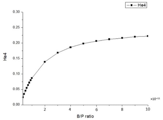
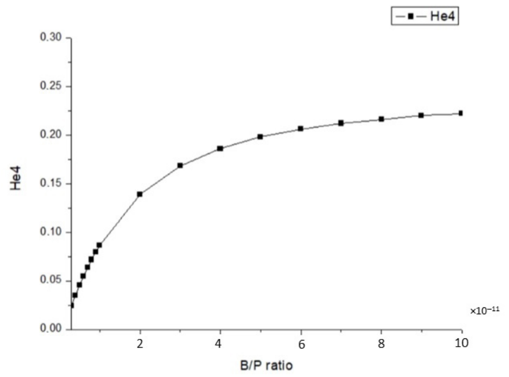
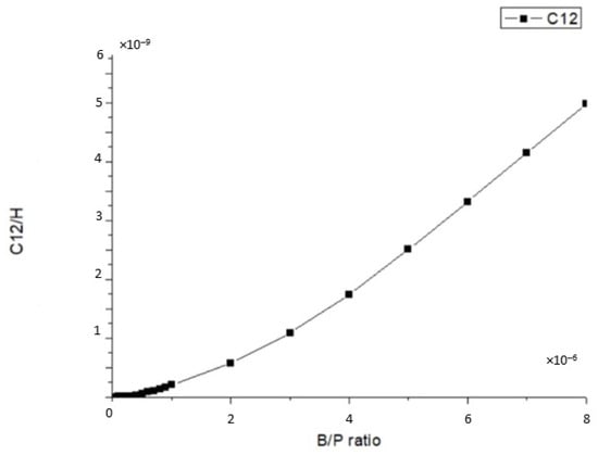
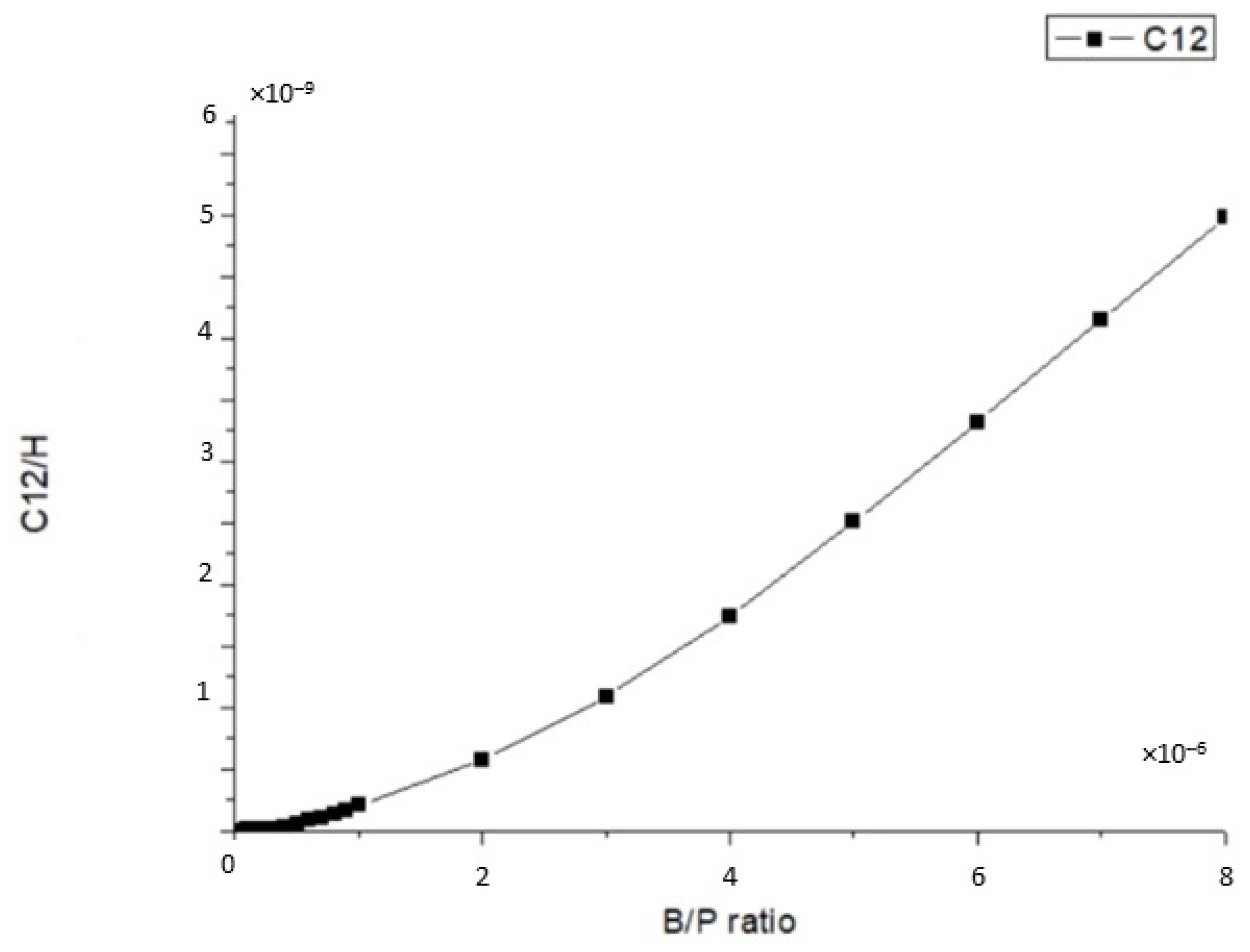
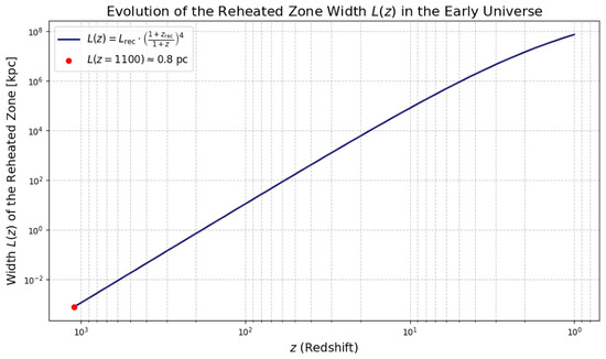
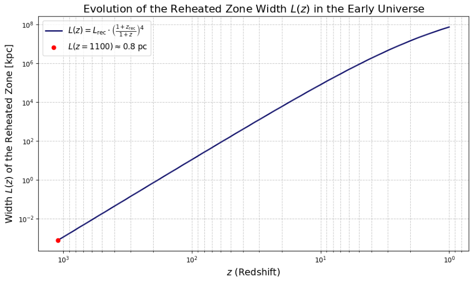
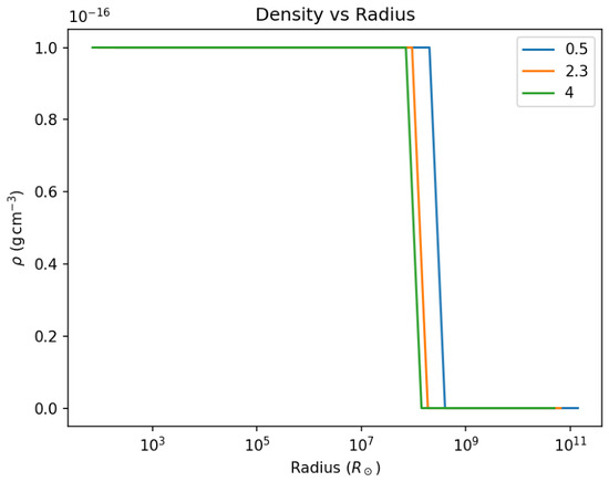
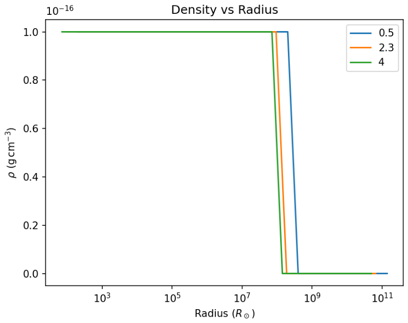
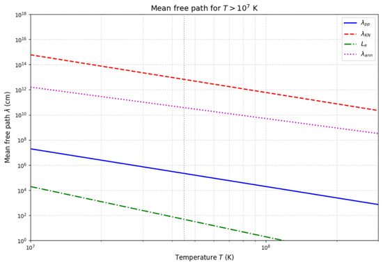
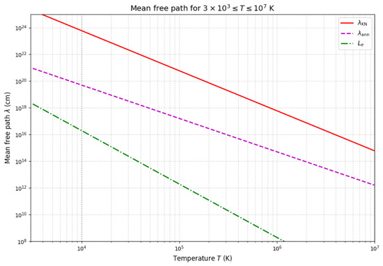

Disclaimer/Publisher’s Note: The statements, opinions and data contained in all publications are solely those of the individual author(s) and contributor(s) and not of MDPI and/or the editor(s). MDPI and/or the editor(s) disclaim responsibility for any injury to people or property resulting from any ideas, methods, instructions or products referred to in the content. |
© 2026 by the authors. Licensee MDPI, Basel, Switzerland. This article is an open access article distributed under the terms and conditions of the Creative Commons Attribution (CC BY) license.