The Investigation of Fault Behaviors and Locations in Hybrid Multiterminal HVDC System Integrated with Renewable Energy Sources

Abstract

The study of hybrid multiterminal high-voltage direct current (HVDC) systems revealed different outcomes regarding their performance under fault conditions. Previous research showed that under the fault conditions, the high-voltage direct current (HVDC) voltage experienced a drop to zero, accompanied by a reverse overshoot. In this paper, a model that integrates hybrid multiterminal line commutated converters (LCCs) and a voltage source converter (VSC) with an HVDC network is presented. The model has been mathematically formulated and implemented using Matlab/Simulink (R2018b) software to examine its fault behaviors and locations, particularly on the DC line to ground fault, line to line fault, and single line to ground fault across various fault resistance levels. The system consists of a wind energy conversion system, a photovoltaic array, protection scheme, LCC rectifier station, VSC inverter station, inverter control, AC filters, a distributed parameter transmission line for the HVDC transmission line, a three-phase inductor-capacitor (LC) filter, and a three-phase transformer. The findings indicated that during the scenario of an 8 ohms of resistance under a single line to ground fault, phase A of the inverter AC grid voltage decreased from its operational level. Meanwhile, the voltage across the DC line increased, accompanied by a rise in DC line current. Additionally, calculations of the fault location were determined to be 1.1561 km from the point of reference. This study contributes to the understanding of fault dynamics in HVDC systems, providing essential insights that enhance operational reliability and efficiency in power transmission networks.

1. Introduction

In recent years, the integration of photovoltaic and wind energy conversion systems into a multiterminal HVDC network has garnered significant attention and momentum within the power sector [1,2,3]. This shift towards renewable energy sources not only aligns with global efforts [4] to reduce carbon emissions [5,6,7] and combat climate change but also reflects a broader recognition of the necessity for sustainable energy solutions in an increasingly energy-dependent world. However, though promising, this integration presents a range of complex challenges, particularly concerning faulty events within the system. As such, modeling of hybrid renewable energy systems with HVDC becomes important for understanding their operational dynamics, evaluating performance metrics, and predicting energy generation capabilities within the existing power grid framework. In recent research conducted by Hossain et al. [8], an analysis of single line to ground fault in an HVDC network revealed their behavior under operating conditions. Specifically, the authors observed a notable phenomenon distinct of phase A at the inverter end, where a significant voltage drop occurred during an incident of a single line to ground fault. In contrast, the other phases, namely B and C, exhibited stability with no fluctuations in voltage despite a gradual increase in the HVDC link voltage at an 80% level. Hossain et al. [8] extended their investigation to a lower operational performance level—specifically, 50% recorded a different response in grid voltage of phase A. It was identified that the outcomes for grid voltage not only increased to 0.5 per unit (p.u.), but the HVDC link voltage itself had minor disturbance with oscillation. Notably, the disturbance was considerably less pronounced compared with the observations at 80% performance. An aspect of Hossain et al.’s [8] work lies in the apparent omission of fault resistance in their models, and its effects on the rectifier end of the system. The lack of these variables prompts uncertainty about the behavior of grid currents at the inverter end under the fault condition, a crucial consideration for power system dynamics during single line to ground faults. Understanding whether this current will collapse or rise presents vital implications for the reliability and stability of power systems, particularly in the context of fault management. Xu et al.’s [9] research investigated the capacity of a pumped storage power plant to help mitigate power quality issues stemming from renewable energy sources. Their findings indicated that the use of pumped storage substantially lessens the instability and variability associated with renewable energy output, thereby fostering higher levels of renewable integration into the energy grid. By serving as a buffer against fluctuations, they claimed that a pumped storage power plant facilitates greater energy consumption from renewable resources that align with sustainability goals. Furthermore, they also added that the pump storage power plant enhances the security and resilience of the power system, ensuring that fluctuations in production do not compromise the integrity of power delivery. However, although their conclusions appear valuable, they warrant a critical examination. The absence of detailed behavior concerning the impact of electrical faults on the performance and stability of the proposed model is a notable limitation of their research. In power systems, faults such as single line to ground, double line to ground, and three-phase to ground faults can create severe disruptions [10,11,12], potentially undermining the advantages offered by pumped storage and renewable energy integration. The research conducted by Liu et al. [13] presented a fault ride-through strategy modified for hybrid HVDC systems, and this strategy was said to influence the controllable line-commutated converter positioned at the receiving end of the HVDC system. The authors highlighted that the implementation of the controllable line-commutated converter facilitated forced commutation, which was instrumental in maintaining stable operational conditions during fault events. In their investigation, Liu et al. proposed a specific fault scenario characterized by a single line to ground fault that would exhibit a resistance of 8 ohms, with a duration of 0.1 s at the receiving terminal. The outcomes of their research compellingly showed that under the fault conditions, the direct current (DC) voltage experienced a significant drop to zero, accompanied by a notable reverse overshoot. However, while these findings provided insights into the behavior of the HVDC system during the fault, the authors did not delineate the precise reactions of the receiving-end alternating current (AC) system within the affected phase. In another research, Liu et al. [14] claimed that the transmission overvoltage is challenging to suppress and evaluate due to the interaction between line-commutated converter high-voltage direct current (LCC-HVDC) systems and renewable energy plants under various operational conditions. The authors asserted that they were able to achieve the transmission overvoltage at the end of the sending, which was influenced by the interaction between renewable energy plants and HVDC. However, the authors ignored examining the system’s behavior under fault conditions, such as a single line to ground fault, and whether the system will remain efficient, reliable, and capable of recovering from such a fault once it is cleared. A research by Su et al. [15] proposed an energy-coordinated control that utilizes the receiving-end converter as an energy buffer. Their results showed that the surface mount capacitor voltages of the DC chopper and the receiving-end converter, the DC-link voltage, and the internal energy fluctuation of the receiving-end converter are all maintained within allowable limits, thereby ensuring reliable and economic fault ride-through operation. However, the authors ignored the single line to ground fault at the receiving end of the AC system. Another research of Yang et al. [16] focused on various power generation methods by providing insights into the operational dynamics of a hybrid multiterminal power system. Their findings revealed that a reduction in the active power output from the thermal power plant will lead to a greater disparity in the active power output ratio between the wind and solar generation components, and their observation underscores the delicate balance required in hybrid systems and illustrates the complexity of managing multiple energy sources to ensure reliability and efficiency in power delivery. Furthermore, Shuo Yang et al. [16] claimed that when the active power output from the thermal power plant dips below a predetermined p.u. threshold, operational challenge will arise. At this point in line, when the active power outputs from both wind and photovoltaic systems are equivalent, the system that was configured under vector current control would exhibit significant limitations. Nevertheless, the absence of the faulty condition will highlight an area that will necessitate further exploration, particularly in light of the susceptibility of power transmission systems to disturbances. The question that is of concern is: how does the proposed hybrid multiterminal system function when subjected to a single line to ground fault condition? Sahraoui et al. [17] embarked on a study that sought to unveil the operational efficiency benefits that such integrations can render. Their research not only provided insights into how these systems function but also suggested that they could deliver a more reliable signal output. However, the study did not produce an aspect regarding the potential implications of fault conditions on the hybrid power system. It can be asserted that without a fault analysis that investigates the system’s reaction during a single line to ground fault event, the robustness and resilience of the proposed system design could be called into question. This oversight raises important concerns about the reliability of such systems, where fault conditions are a recurring and unavoidable reality. Furthermore, understanding frequency and power stability is vital for the operational integrity of electrical power systems [18,19,20]. Frequency deviation and power oscillations can occur due to various factors, including sudden changes in load, generation, and system fault. When deviations occur, they can result in disruptive oscillations that may lead to system instability or even blackouts, underscoring the need for thorough investigations into these phenomena. The research conducted by Iqbal et al. [21] concentrated on the critical phenomena of frequency deviation and power oscillation within the electrical system, aiming to shed light on the impacts of faults on grid stability and performance. In their study, the researchers [21] introduced a simulated fault that persisted for a duration of 0.5 s, a period to observe the dynamic responses of the system under duress. The findings from their investigation indicated that during the occurrence of the fault, the alternating current (AC) grid voltages and currents decreased to levels approaching zero, which represent a severe disruption in power delivery. Concurrently, the power output of the system was found to collapse entirely, dropping to zero. In addition to their findings, the frequency of the electrical system exhibited a downward trend, further accentuated by undesirable oscillations. However, an important limitation of their research is the lack of specificity regarding the type of fault that was introduced into the simulation. It remains unclear whether the fault was single line to ground, double line to ground, or three-phase to ground faults or if there was any clarification regarding the resistance value attributed to the fault itself. This omission represents a significant gap in their study. In a research conducted by Ikotun et al. [22], the authors limit their focus on double line to ground fault at the point of common coupling, considering various fault resistances at the inverter end. However, they did not explore how single line to ground fault would behave within the system as well as line to line fault at the rectifier end. In separate research, Ikotun et al. [23] focused on a DC line to ground fault and showed its impact on the entire system from the rectifier end to the DC link as well as the inverter end. In their simulation results, the authors claimed that at the inverter end, the AC grid voltages reduce along with AC grid currents. However, they neglect to consider the effects of a single line to ground fault at the inverter end and line to line fault at the rectifier end. Nevertheless, previous research indicates that issues can arise within the system during a single line to ground fault at the end of the inverter of the AC system, claiming that the DC voltage experienced a significant drop to zero, accompanied by a notable reverse overshot. It can be argued that in this study, the 8 ohms fault resistance used during the single line to ground fault scenario that results in the AC grid voltage of the affected phase will reduce, while the voltages of the other phases will remain at standard levels. In addition, the AC grid current for the affected phase will decrease at the inverter side, while the currents for the unaffected phases will continue to exhibit stability. Concurrently, the DC line voltage will increase, leading to an increase in DC line current. At the rectifier end of the system, the status of the AC grid voltages across phases A, B, and C will remain stable, along with the corresponding AC grid currents. The present study investigates a single line to ground fault occurring at the inverter end, DC line to ground fault, and line to line fault at the rectifier end of the AC system and examines their effects at the DC link, rectifier end, and inverter end of the AC system. The analysis includes detailed simulations that consider various fault resistance values and fault locations. Furthermore, a model of an HVDC system integrated with photovoltaic and wind energy conversion systems are mathematically modeled and implemented using Matlab/Simulink software. The simulation results for these models are presented later in the paper.

2. System Modeling

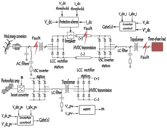
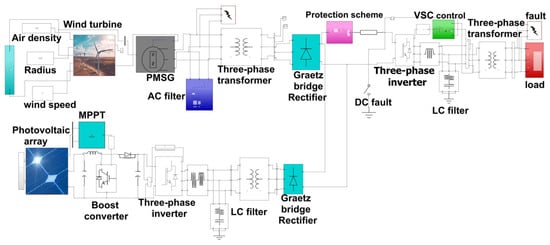
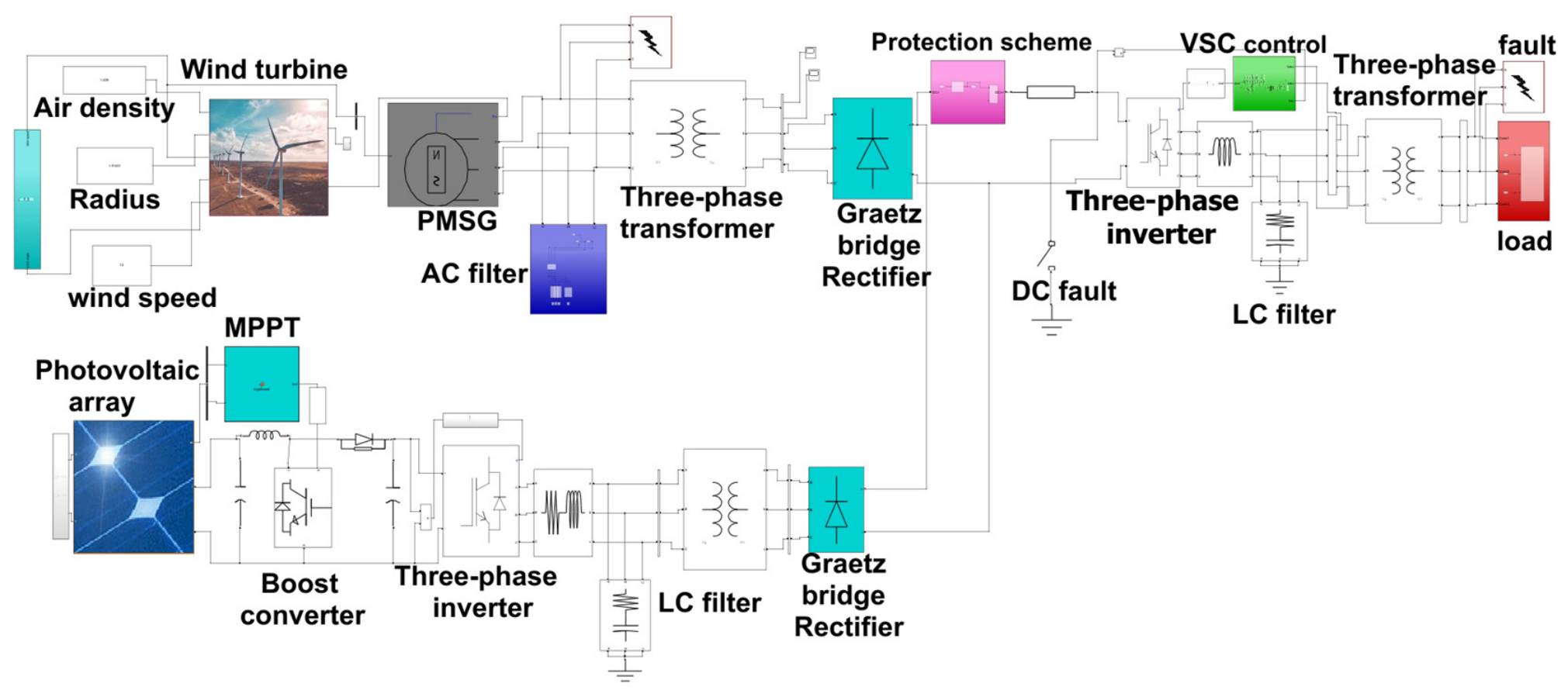
Figure 1 shows a framework in which renewable energy sources are interconnected through line-commutated converters (LCCs) alongside a voltage source converter (VSC) HVDC system. This study focuses on a system that incorporates a wind energy conversion system, photovoltaic array, LCC rectifier station, VSC inverter station, protection scheme, AC filters located at the rectifier side, inverter control, a distributed parameter transmission line designed for the HVDC transmission line, a three-phase LC filter positioned at the inverter side, and a three-phase transformer.

Figure 1. Proposed diagram of photovoltaic/wind energy conversion grid, connected via HVD.

2.1. Wind Energy Conversion System

The wind energy conversion system facilitates the conversion of kinetic energy from wind into mechanical energy, which was then transformed into electrical energy. The typical wind energy conversion system consists of several key components: the rotor, the nacelle, the tower, and control and electrical systems. The rotor, made up of blades, captures the wind’s kinetic energy. As the blades rotate, they turn the rotor, which is connected to a generator within the nacelle. The nacelle houses the generator, gearbox, and other critical components, allowing for efficient energy conversion. The tower supports the nacelle and rotor, elevating them to a height where wind speeds are generally higher. Modern wind turbines employ sensors and software to adjust the pitch of the blades and the yaw of the turbine to align with wind direction, maintaining maximum efficiency. The equation that governs the power output of a wind turbine can be expressed as:

$${\mathrm{P}}_{\mathrm{m}\mathrm{O}\mathrm{p}}={\displaystyle \frac{1}{2}}{\mathrm{\rho }}_{\mathrm{A}\mathrm{d}}{\mathrm{A}}_{\mathrm{s}\mathrm{A}}{\mathrm{C}}_{\mathrm{p}\mathrm{C}}\left({\mathrm{\lambda }}_{\mathrm{T}\mathrm{s}\mathrm{R}},{\mathrm{\beta }}_{\mathrm{B}\mathrm{p}\mathrm{a}}\right){\mathrm{v}}_{\mathrm{w}\mathrm{S}}^3$$

(1)

where ${\mathrm{P}}_{\mathrm{m}\mathrm{O}\mathrm{p}}$ is the mechanical output power (Watts); ${\mathrm{\rho }}_{\mathrm{A}\mathrm{d}}$ represents the air density, typically 1.225 $\mathrm{k}\mathrm{g}/{\mathrm{m}}^3$; ${\mathrm{A}}_{\mathrm{s}\mathrm{A}}$ refers to the swept area of the blades, which is calculated as $\mathrm{\pi }{\mathrm{R}}^2$ (the R represents the blade radius); ${\mathrm{\lambda }}_{\mathrm{T}\mathrm{s}\mathrm{R}}$ is the tip speed ratio; ${\mathrm{\beta }}_{\mathrm{B}\mathrm{p}\mathrm{a}}$ refers to the blade pitch angle; and ${\mathrm{v}}_{\mathrm{W}\mathrm{s}}$ is the wind speed $\left(\mathrm{m}/\mathrm{s}\right)$. However, the power output can be given as in terms of torque (T) utilizing Equation (2)

$${\mathrm{P}}_{\mathrm{m}\mathrm{O}\mathrm{p}}={\mathrm{T}}_{\mathrm{m}\mathrm{T}}{\mathrm{\omega }}_{\mathrm{A}\mathrm{v}}$$

(2)

where ${\mathrm{T}}_{\mathrm{m}\mathrm{T}}$ refers to the mechanical torque, expressed in $\mathrm{N}-\mathrm{m}$; ${\mathrm{\omega }}_{\mathrm{A}\mathrm{v}}$ represents angular velocity of the wind turbine rotor $\left(\mathrm{r}\mathrm{a}\mathrm{d}/\mathrm{s}\right)$. The important parameter in determining the mechanical torque and power output of the turbine is the tip speed ratio, and the equation is expressed as

$${\mathrm{\lambda }}_{\mathrm{T}\mathrm{s}\mathrm{R}}={\displaystyle \frac{{\mathrm{\omega }}_{\mathrm{A}\mathrm{v}}\mathrm{R}}{{\mathrm{v}}_{\mathrm{W}\mathrm{s}}}}$$

(3)

For the power coefficient, $\left({\mathrm{C}}_{\mathrm{p}\mathrm{C}}\right)$ also depends on the pitch angle and tip speed ratio, and the equation is expressed as

$${\mathrm{C}}_{\mathrm{p}\mathrm{C}}\left({\mathrm{\lambda }}_{\mathrm{T}\mathrm{s}\mathrm{R}},{\mathrm{\beta }}_{\mathrm{B}\mathrm{p}\mathrm{a}}\right)={\mathrm{c}}_1\left({\displaystyle \frac{{\mathrm{c}}_2}{{\mathrm{\lambda }}_{\mathrm{i}}}}-{\mathrm{c}}_3{\mathrm{\beta }}_{\mathrm{B}\mathrm{p}\mathrm{a}}-{\mathrm{c}}_4\right){\mathrm{e}}^{{\displaystyle \frac{{\mathrm{c}}_5}{{\mathrm{\lambda }}_{\mathrm{i}}}}}+{\mathrm{c}}_6{\mathrm{\lambda }}_{\mathrm{T}\mathrm{s}\mathrm{R}}$$

(4)

where

$${\displaystyle \frac{1}{{\mathrm{\lambda }}_{\mathrm{i}}}}={\displaystyle \frac{1}{{\mathrm{\lambda }}_{\mathrm{T}\mathrm{s}\mathrm{R}}+0.08{\mathrm{\beta }}_{\mathrm{B}\mathrm{p}\mathrm{a}}}}-{\displaystyle \frac{0.035}{{\mathrm{\beta }}_{\mathrm{B}\mathrm{p}\mathrm{a}}^3+1}}$$

(5)

Furthermore, the design of permanent magnet synchronous generators (PMSGs) involves direct coupling of the turbine rotor and the generator, allowing the turbine to directly drive the generator without the intermediary mechanical components typically found in conventional systems [24,25]. This configuration reduces friction and energy losses associated with gearboxes, leading to increased operational efficiency. As noted by [26,27], the elimination of such mechanical components reduces the risk of failure, significantly mitigates downtime, and consequently enhances the overall reliability of the wind energy system. The direct drive PMSGs present a significant advancement in wind energy technology, which leads to eliminating the need for a gearbox; these systems minimize maintenance time and costs [28,29]. Gearbox failures are associated with over 19% of the downtime experienced in wind turbine generators [30], underscoring the reliability advantages of PMSGs. Moreover, the design of PMSGs eliminates rotor currents and, subsequently, copper losses in the rotor circuit, which contributes to their superior efficiency [31,32]. The equations for modeling the generator are the ones for the d-axis and q-axis current, which can be expressed as

$${\displaystyle \frac{\mathrm{d}{\mathrm{i}}_{\mathrm{d}\mathrm{S}\mathrm{C}}}{\mathrm{d}\mathrm{t}}}={\displaystyle \frac{1}{{\mathrm{L}}_{\mathrm{d}\mathrm{S}\mathrm{I}}}}\left[{\mathrm{e}}_{\mathrm{d}\mathrm{S}\mathrm{V}}+\mathrm{p}{\mathrm{\omega }}_{\mathrm{a}\mathrm{f}}{\mathrm{L}}_{\mathrm{q}\mathrm{S}\mathrm{I}}{\mathrm{i}}_{\mathrm{q}\mathrm{S}\mathrm{C}}-{\mathrm{R}}_{\mathrm{d}\mathrm{S}\mathrm{R}}{\mathrm{i}}_{\mathrm{d}\mathrm{S}\mathrm{C}}\right]$$

(6)

$${\displaystyle \frac{\mathrm{d}{\mathrm{i}}_{\mathrm{q}\mathrm{S}\mathrm{C}}}{\mathrm{d}\mathrm{t}}}={\displaystyle \frac{1}{{\mathrm{L}}_{\mathrm{q}\mathrm{S}\mathrm{I}}}}\left[{\mathrm{e}}_{\mathrm{q}\mathrm{S}\mathrm{V}}+\mathrm{p}{\mathrm{\omega }}_{\mathrm{a}\mathrm{f}}\left({\mathrm{L}}_{\mathrm{d}\mathrm{S}\mathrm{I}}{\mathrm{i}}_{\mathrm{d}\mathrm{S}\mathrm{C}}+{\mathrm{M}}_{\mathrm{M}\mathrm{I}}{\mathrm{i}}_{\mathrm{R}\mathrm{C}}\right)-{\mathrm{R}}_{\mathrm{q}\mathrm{S}\mathrm{R}}{\mathrm{i}}_{\mathrm{q}\mathrm{S}\mathrm{C}}\right]$$

(7)

For the electromagnetic torque, $\left({\mathrm{T}}_{\mathrm{e}\mathrm{T}}\right)$ can be expressed as

$${\mathrm{T}}_{\mathrm{e}\mathrm{T}}=1.5\mathrm{p}\left[{\mathrm{\varphi }}_{\mathrm{f}\mathrm{L}}{\mathrm{i}}_{\mathrm{q}\mathrm{S}\mathrm{C}}+\left({\mathrm{L}}_{\mathrm{d}\mathrm{S}\mathrm{I}}-{\mathrm{L}}_{\mathrm{q}\mathrm{S}\mathrm{I}}\right){\mathrm{i}}_{\mathrm{d}\mathrm{S}\mathrm{C}}{\mathrm{i}}_{\mathrm{q}\mathrm{S}\mathrm{C}}\right]$$

(8)

where ${\mathrm{L}}_{\mathrm{d}\mathrm{S}\mathrm{I}}$ and ${\mathrm{L}}_{\mathrm{q}\mathrm{S}\mathrm{I}}$ refer to d-axis and q-axis stator inductances; ${\mathrm{i}}_{\mathrm{d}\mathrm{S}\mathrm{C}}$ and ${\mathrm{i}}_{\mathrm{q}\mathrm{S}\mathrm{C}}$ represent the d-axis and q-axis stator currents; ${\mathrm{\varphi }}_{\mathrm{f}\mathrm{L}}$ represents flux linkage; $\mathrm{p}$ refers to the number of pole pairs in PMSG; ${\mathrm{M}}_{\mathrm{M}\mathrm{I}}$ is the mutual inductance; ${\mathrm{i}}_{\mathrm{R}\mathrm{C}}$ stands for the equivalent rotor current; ${\mathrm{R}}_{\mathrm{d}\mathrm{S}\mathrm{R}}$ and ${\mathrm{R}}_{\mathrm{q}\mathrm{S}\mathrm{R}}$ refer to the d-axis and q-axis stator resistances; ${\mathrm{e}}_{\mathrm{d}\mathrm{S}\mathrm{V}}$ and ${\mathrm{e}}_{\mathrm{q}\mathrm{S}\mathrm{V}}$ are the d-axis and q-axis stator voltages; and ${\mathrm{\omega }}_{\mathrm{a}\mathrm{f}}$ refers to the electric angular frequency of the generator. In addition, the salient pole was introduced due to the low-speed operation of PMSG in wind turbines, and for the salient pole rotors, the d-axis and q-axis of the stator induction is expressed as

$${\mathrm{L}}_{\mathrm{d}\mathrm{S}\mathrm{I}}={\displaystyle \frac{{\mathrm{L}}_{\mathrm{d}\_\mathrm{M}\mathrm{a}}}{2}}$$

(9)

$${\mathrm{L}}_{\mathrm{q}\mathrm{S}\mathrm{I}}={\displaystyle \frac{{\mathrm{L}}_{\mathrm{d}\_\mathrm{M}\mathrm{i}}}{2}}$$

(10)

where ${\mathrm{L}}_{\mathrm{d}\_\mathrm{M}\mathrm{a}}$ and ${\mathrm{L}}_{\mathrm{d}\_\mathrm{M}\mathrm{i}}$ represent the maximum d-axis inductance and minimum q-axis inductance.

2.2. Photovoltaic System

Photovoltaic systems operate on the principle of the photovoltaic effect, where certain materials generate electricity when exposed to light [33,34]. Typically composed of solar panels made from silicon, these systems use semiconductor materials that exhibit the photovoltaic effect [35]. When photons from sunlight hit the solar cells, they excite electrons, creating an electric current [36]. The modeling of a photovoltaic cell is governed by the following equations:

For the photocurrent $\left({\mathrm{I}}_{\mathrm{p}\mathrm{h}\mathrm{t}}\right)$

$${\mathrm{I}}_{\mathrm{p}\mathrm{h}\mathrm{t}}=\left[{\mathrm{I}}_{\mathrm{s}\mathrm{C}}+{\mathrm{K}}_{\mathrm{i}\mathrm{T}}\left(\mathrm{T}-{\mathrm{T}}_{\mathrm{r}\mathrm{e}\mathrm{f}\mathrm{T}}\right)\right]\times {\displaystyle \frac{\mathrm{G}}{1000}}$$

(11)

For the reverse saturation current, $\left({\mathrm{I}}_{\mathrm{r}\mathrm{s}\mathrm{C}}\right)$ is given as

$${\mathrm{I}}_{\mathrm{r}\mathrm{s}\mathrm{C}}={\displaystyle \frac{{\mathrm{I}}_{\mathrm{s}\mathrm{C}}}{\exp \left(\frac{{\mathrm{q}}_{\mathrm{e}\mathrm{C}}\times {\mathrm{V}}_{\mathrm{o}\mathrm{C}}}{{\mathrm{N}}_{\mathrm{C}\mathrm{s}}\times {\mathrm{a}}_{\mathrm{D}}\times \mathrm{k}\times \mathrm{T}}\right)-1}}$$

(12)

The equation for the saturation current $\left({\mathrm{I}}_{\mathrm{O}\mathrm{s}\mathrm{c}}\right)$ can be expressed as

$${\mathrm{I}}_{\mathrm{O}\mathrm{s}\mathrm{c}}={\mathrm{I}}_{\mathrm{r}\mathrm{s}\mathrm{C}}{\left({\displaystyle \frac{\mathrm{T}}{{\mathrm{T}}_{\mathrm{r}\mathrm{e}\mathrm{f}\mathrm{T}}}}\right)}^3\exp \left({\displaystyle \frac{{\mathrm{q}}_{\mathrm{e}\mathrm{c}}\times {\mathrm{E}}_{\mathrm{g}\mathrm{E}}}{{\mathrm{a}}_{\mathrm{D}}\times \mathrm{k}}}\left({\displaystyle \frac{1}{{\mathrm{T}}_{\mathrm{r}\mathrm{e}\mathrm{f}\mathrm{T}}}}-{\displaystyle \frac{1}{\mathrm{T}}}\right)\right)$$

(13)

However, the module output current $\left(\mathrm{I}\right)$ is expressed as

$$\mathrm{I}={\mathrm{I}}_{\mathrm{p}\mathrm{h}\mathrm{t}}-{\mathrm{I}}_{\mathrm{O}\mathrm{s}\mathrm{c}}\left[\exp \left({\displaystyle \frac{\mathrm{V}+\mathrm{I}{\mathrm{R}}_{\mathrm{s}\mathrm{e}\mathrm{r}}}{{\mathrm{N}}_{\mathrm{C}\mathrm{s}}\times {\mathrm{a}}_{\mathrm{D}}\times {\mathrm{V}}_{\mathrm{t}\mathrm{h}\mathrm{V}}}}-1\right)\right]-{\displaystyle \frac{\mathrm{V}+\mathrm{I}{\mathrm{R}}_{\mathrm{s}\mathrm{e}\mathrm{r}}}{{\mathrm{R}}_{\mathrm{s}\mathrm{h}\mathrm{R}}}}$$

(14)

where ${\mathrm{I}}_{\mathrm{s}\mathrm{C}}$ is the short circuit current; T is the operating temperature; G refers to the solar irradiance (W/m²); ${\mathrm{K}}_{\mathrm{i}\mathrm{T}}$ represents the short circuit temperature coefficient; ${\mathrm{T}}_{\mathrm{r}\mathrm{e}\mathrm{f}\mathrm{T}}$ is the reference temperature in Kelvin (K); ${\mathrm{q}}_{\mathrm{e}\mathrm{C}}$ is the electron charge (1.602 × 10⁻¹⁹ C); ${\mathrm{V}}_{\mathrm{t}\mathrm{h}\mathrm{V}}$ represent the thermal voltage; ${\mathrm{N}}_{\mathrm{C}\mathrm{s}}$ is the number of cells in series; ${\mathrm{R}}_{\mathrm{s}\mathrm{e}\mathrm{r}}$ refers to the series resistance; ${\mathrm{a}}_{\mathrm{D}}$ is the diode ideality factor; ${\mathrm{R}}_{\mathrm{s}\mathrm{h}\mathrm{R}}$ refers to the shunt resistance; ${\mathrm{E}}_{\mathrm{g}\mathrm{E}}$ represents the bandgap energy of the semiconductor; and $\mathrm{k}$ is the Boltzmann constant (1.3806 × 10⁻²³ J/K).

2.3. LCC Rectifier Station

The six-pulse Graetz bridge converter is one of the most widely used configurations in converting AC to DC. Its design consists of six diodes arranged in a bridge configuration, allowing it to rectify three-phase AC power into a unidirectional DC [37]. However, its simplicity in operation contributes to its widespread use in both traditional and modern HVDC implementations. The significant characteristics of this configuration is that it produces six pulses of output per cycle, leading to smoother DC output compared with other configurations with fewer pulses, and the equation for output voltage can be expressed as

$${\mathrm{V}}_{\mathrm{d}\mathrm{c}\mathrm{O}}={\mathrm{V}}_{\mathrm{d}\mathrm{o}}\cos {\mathrm{\alpha }}_{\mathrm{f}\mathrm{A}}-{\mathrm{R}}_{\mathrm{c}\mathrm{R}}{\mathrm{I}}_{\mathrm{d}\mathrm{c}\mathrm{C}}={\displaystyle \frac{{\mathrm{V}}_{\mathrm{d}\mathrm{o}}}{2}}\left(\cos {\mathrm{\alpha }}_{\mathrm{f}\mathrm{A}}+\cos \left({\mathrm{\alpha }}_{\mathrm{f}\mathrm{A}}+{\mathrm{\mu }}_{\mathrm{o}\mathrm{A}}\right)\right)$$

(15)

where ${\mathrm{\alpha }}_{\mathrm{f}\mathrm{A}}$ refers to the firing angle, ${\mathrm{I}}_{\mathrm{d}\mathrm{c}\mathrm{C}}$ is the DC line current, ${\mathrm{\mu }}_{\mathrm{o}\mathrm{A}}$ represents the overlap angle, and ${\mathrm{R}}_{\mathrm{c}\mathrm{R}}$ refers to the commutation resistance, and the equation is given as ${\displaystyle \frac{3{\mathrm{\omega }}_{\mathrm{a}\mathrm{v}}{\mathrm{L}}_{\mathrm{c}\mathrm{I}}}{\mathrm{\pi }}}$. The ${\mathrm{L}}_{\mathrm{c}\mathrm{I}}$ is the transformer leakage inductance. Furthermore, the LC Graetz bridge absorbs power (reactive), which is presented as Q_dp continuously, and it operates at a Lagging power factor. The reactive power equation is expressed as

$${\mathrm{Q}}_{\mathrm{d}\mathrm{P}}={\mathrm{P}}_{\mathrm{d}\mathrm{c}\mathrm{P}}\tan \mathrm{\varphi }={\mathrm{V}}_{\mathrm{d}\mathrm{c}\mathrm{O}}{\mathrm{I}}_{\mathrm{d}\mathrm{c}\mathrm{C}}\tan \left(\arccos \left(\cos \mathrm{\alpha }-{\displaystyle \frac{{\mathrm{R}}_{\mathrm{c}\mathrm{R}}{\mathrm{I}}_{\mathrm{d}\mathrm{c}\mathrm{C}}}{{\mathrm{V}}_{\mathrm{d}\mathrm{o}}}}\right)\right)$$

(16)

For the active power, $\left({\mathrm{P}}_{\mathrm{d}\mathrm{c}\mathrm{P}}\right)$ delivered to the DC network is expressed as

$${\mathrm{P}}_{\mathrm{d}\mathrm{c}\mathrm{P}}={\mathrm{V}}_{\mathrm{d}\mathrm{c}\mathrm{O}}{\mathrm{I}}_{\mathrm{d}\mathrm{c}\mathrm{C}}$$

(17)

2.4. VSC Inverter Station

The voltage source inverter is an important component of the HVDC system that helps to convert direct current into alternating current. The IGBT is a power semiconductor device used in inverters due to its high efficiency, capacity to handle large power levels, and fast switching times. However, the incorporation of antiparallel diodes in IGBTs is necessary for ensuring the proper operation of the inverter when it comes to managing reverse current flow and also protecting the device from voltage spikes. Understanding the equations governing the operation of voltage source inverters with IGBT anti-parallel diodes is important for analyzing their performance in a multiterminal HVDC system and is expressed as.

For the IGBT conduction loss

$${\mathrm{P}}_{\mathrm{I}\mathrm{G}\mathrm{B}\mathrm{T}.\mathrm{c}\mathrm{o}\mathrm{n}\mathrm{R}}={\mathrm{V}}_{\mathrm{t}\mathrm{h}\mathrm{r}\mathrm{e}\mathrm{s}.\mathrm{V}\mathrm{o}\mathrm{l}\mathrm{t}}{\mathrm{I}}_{\mathrm{a}\mathrm{v}\mathrm{g}.\mathrm{T}}+{\mathrm{r}}_{\mathrm{s}\mathrm{l}.\mathrm{d}}.{\mathrm{I}}_{\mathrm{R}\mathrm{M}\mathrm{S}}^2$$

(18)

where ${\mathrm{P}}_{\mathrm{I}\mathrm{G}\mathrm{B}\mathrm{T}.\mathrm{c}\mathrm{o}\mathrm{n}\mathrm{R}}$ is the conduction losses of the IGBT, ${\mathrm{V}}_{\mathrm{t}\mathrm{h}\mathrm{r}\mathrm{e}\mathrm{s}.\mathrm{V}\mathrm{o}\mathrm{l}\mathrm{t}}$ refers to threshold voltage, ${\mathrm{I}}_{\mathrm{a}\mathrm{v}\mathrm{g}.\mathrm{T}}$ represents the average current, ${\mathrm{r}}_{\mathrm{s}\mathrm{l}.\mathrm{d}}$ is the slope on-state resistance, and ${\mathrm{I}}_{\mathrm{R}\mathrm{M}\mathrm{S}}$ refers to the root mean square current over a cycle and the conduction losses for the diode

$${\mathrm{P}}_{\mathrm{D}\mathrm{I}\mathrm{O}\mathrm{D}\mathrm{E}.\mathrm{c}\mathrm{o}\mathrm{n}\mathrm{R}}={\mathrm{V}}_{\mathrm{t}\mathrm{h}\mathrm{r}\mathrm{e}\mathrm{s}.\mathrm{V}\mathrm{o}\mathrm{l}\mathrm{t}\mathrm{D}}{\mathrm{I}}_{\mathrm{a}\mathrm{v}\mathrm{g}.\mathrm{D}}+{\mathrm{r}}_{\mathrm{s}\mathrm{l}.\mathrm{d}}.{\mathrm{I}}_{\mathrm{R}\mathrm{M}\mathrm{S}}^2$$

(19)

The switching loss and the recovering loss of the IGBT and anti-parallel diode are expressed as

$${\mathrm{P}}_{\mathrm{I}\mathrm{G}\mathrm{B}\mathrm{T}.\mathrm{s}\mathrm{w}\mathrm{t}\mathrm{h}}={\mathrm{f}}_{\mathrm{s}\mathrm{w}\mathrm{t}\mathrm{h}\_\mathrm{L}}\times \left({\mathrm{E}}_{\mathrm{T}\_\mathrm{o}\mathrm{n}}+{\mathrm{E}}_{\mathrm{T}\_\mathrm{o}\mathrm{f}\mathrm{f}}\right)\times \left({\displaystyle \frac{{\mathrm{V}}_{\mathrm{d}\mathrm{c}\mathrm{O}}}{{\mathrm{V}}_{\mathrm{d}\mathrm{c}\mathrm{O}\_\mathrm{v}}}}\right)$$

(20)

And

$${\mathrm{P}}_{\mathrm{D}\mathrm{I}\mathrm{O}\mathrm{D}\mathrm{E}.\mathrm{s}\mathrm{w}\mathrm{t}\mathrm{h}}={\mathrm{f}}_{\mathrm{s}\mathrm{w}\mathrm{t}\mathrm{h}\_\mathrm{L}}\times {\mathrm{E}}_{\mathrm{d}\mathrm{r}\_\mathrm{e}\mathrm{n}\mathrm{L}}\times \left({\displaystyle \frac{{\mathrm{V}}_{\mathrm{d}\mathrm{c}\mathrm{O}}}{{\mathrm{V}}_{\mathrm{d}\mathrm{c}\mathrm{O}\_\mathrm{v}}}}\right)$$

(21)

where ${\mathrm{f}}_{\mathrm{s}\mathrm{w}\mathrm{t}\mathrm{h}\_\mathrm{L}}$ is the switching frequency of the inverter side, ${\mathrm{E}}_{\mathrm{T}\_\mathrm{o}\mathrm{n}}$ refers to turn-on energy losses of the IGBT per pulse, ${\mathrm{E}}_{\mathrm{T}\_\mathrm{o}\mathrm{f}\mathrm{f}}$ represents turn-off energy losses of the IGBT per pulse, and ${\mathrm{E}}_{\mathrm{d}\mathrm{r}\_\mathrm{e}\mathrm{n}\mathrm{L}}$ is the diode reverse recovery energy loss.

2.5. Protection Scheme

The voltage and current protection are important in maintaining the HVDC system integrity during the fault condition. During the fault, the distributed parameters line that were used include inductance and capacitance. These components dictate the sudden rise in DC current, and the monitoring relay was introduced due to the transmission line behavior during short circuit fault; the transient loop equation is expressed as

$${\displaystyle \frac{\mathrm{d}\mathrm{i}\left(\mathrm{t}\right)}{\mathrm{d}\mathrm{t}}}={\displaystyle \frac{{\mathrm{V}}_{\mathrm{d}\mathrm{c}\_\mathrm{V}}-\left({\mathrm{i}}_{\mathrm{i}\mathrm{n}\mathrm{s}\mathrm{t}\_\mathrm{f}\mathrm{C}}(\mathrm{t})\times {\mathrm{R}}_{\mathrm{T}\mathrm{l}\mathrm{o}\mathrm{o}\mathrm{p}\_\mathrm{R}}\left(\mathrm{x}\right)\right)-{\mathrm{V}}_{\mathrm{f}}}{{\mathrm{L}}_{\mathrm{T}\mathrm{l}\mathrm{o}\mathrm{o}\mathrm{p}\_\mathrm{I}\mathrm{n}}\left(\mathrm{x}\right)}}$$

(22)

where ${\mathrm{V}}_{\mathrm{d}\mathrm{c}\_\mathrm{V}}$ refers to the nominal DC voltage, ${\mathrm{i}}_{\mathrm{i}\mathrm{n}\mathrm{s}\mathrm{t}\_\mathrm{f}\mathrm{C}}(\mathrm{t})$ refers to the instantaneous fault current, ${\mathrm{R}}_{\mathrm{T}\mathrm{l}\mathrm{o}\mathrm{o}\mathrm{p}\_\mathrm{R}}\left(\mathrm{x}\right)$ refers to the total resistance up to fault distance, ${\mathrm{L}}_{\mathrm{T}\mathrm{l}\mathrm{o}\mathrm{o}\mathrm{p}\_\mathrm{I}\mathrm{n}}\left(\mathrm{x}\right)$ represents the total resistance up to fault distance, and ${\mathrm{V}}_{\mathrm{v}\mathrm{o}\mathrm{l}\mathrm{t}\_\mathrm{f}}$ is the fault voltage. However, at the onset of the fault inception, the DC line current has not deviated from the balanced state, and this yielded to the initial rate of change of the current equation, which was used in this research

$${\left.{\displaystyle \frac{\mathrm{d}\mathrm{i}}{\mathrm{d}\mathrm{t}}}\right|}_{\mathrm{t}=0^{+}}={\displaystyle \frac{{\mathrm{V}}_{\mathrm{d}\mathrm{c}\_\mathrm{V}}-\left({\mathrm{I}}_{\mathrm{d}\mathrm{c}\_\mathrm{I}}\times \left(\left({\mathrm{r}}_{\mathrm{l}\mathrm{i}\mathrm{n}\mathrm{e}\_\mathrm{r}\mathrm{e}\mathrm{s}}\times \right)+{\mathrm{R}}_{\mathrm{f}\mathrm{a}\mathrm{u}\mathrm{l}\mathrm{t}}\right)\right)}{\left({\mathrm{L}}_{\mathrm{l}\mathrm{i}\mathrm{n}\mathrm{e}\_\mathrm{i}\mathrm{n}\mathrm{d}.}\times {\mathrm{X}}_{\mathrm{d}\mathrm{i}\mathrm{s}\mathrm{t}.}\right)}}\mathrm{A}/\mathrm{s}$$

(23)

Furthermore, overcurrent protection relay uses a coordination safety margin factor $\left({\mathrm{T}}_{\mathrm{s}\mathrm{a}\mathrm{f}\mathrm{e}\mathrm{t}\mathrm{y}\mathrm{M}}\right)$, which triggers when fault current passes the settling threshold typically between 1.2 to 1.5 of the rated operating current even during load variations, and the equation is given as:

$${\mathrm{I}}_{\mathrm{t}\mathrm{h}\mathrm{r}\mathrm{e}\mathrm{s}\mathrm{h}}={\mathrm{T}}_{\mathrm{s}\mathrm{a}\mathrm{f}\mathrm{e}\mathrm{t}\mathrm{y}\mathrm{M}}\times {\mathrm{I}}_{\mathrm{d}\mathrm{c}\_\mathrm{C}}$$

(24)

where ${\mathrm{I}}_{\mathrm{t}\mathrm{h}\mathrm{r}\mathrm{e}\mathrm{s}\mathrm{h}}$ is overcurrent threshold and ${\mathrm{I}}_{\mathrm{d}\mathrm{c}\_\mathrm{C}}$ refers to the nominal DC current and the allowable time delay before isolation, which is given as

$$\Delta {\mathrm{t}}_{\mathrm{t}\mathrm{r}\mathrm{i}\mathrm{p}\_\mathrm{D}}={\displaystyle \frac{\left({\mathrm{T}}_{\mathrm{s}\mathrm{a}\mathrm{f}\mathrm{e}\mathrm{t}\mathrm{y}\mathrm{M}}-1\right)\times {\mathrm{I}}_{\mathrm{d}\mathrm{c}\_\mathrm{I}}\times {\mathrm{L}}_{\mathrm{T}\mathrm{l}\mathrm{o}\mathrm{o}\mathrm{p}\_\mathrm{I}\mathrm{n}}}{{\mathrm{V}}_{\mathrm{d}\mathrm{c}\_\mathrm{V}}-\left({\mathrm{R}}_{\mathrm{T}\mathrm{l}\mathrm{o}\mathrm{o}\mathrm{p}\_\mathrm{R}}\times {\mathrm{I}}_{\mathrm{d}\mathrm{c}\_\mathrm{I}}\right)}}$$

(25)

For the rate of change of voltage, the voltage behavior during fault immediately involved the line wave impedance $\left({\mathrm{T}}_{\mathrm{w}\mathrm{a}\mathrm{v}\mathrm{e}\_\mathrm{i}\mathrm{m}\mathrm{p}.}\right)$, and propagation velocity was used in this research; the equations are expressed as

$${\mathrm{T}}_{\mathrm{w}\mathrm{a}\mathrm{v}\mathrm{e}\_\mathrm{i}\mathrm{m}\mathrm{p}.}=\sqrt{{\displaystyle \frac{{\mathrm{L}}_{\mathrm{l}\mathrm{i}\mathrm{n}\mathrm{e}\_\mathrm{i}\mathrm{n}\mathrm{d}.}}{{\mathrm{C}}_{\mathrm{l}\mathrm{i}\mathrm{n}\mathrm{e}\_\mathrm{c}\mathrm{a}\mathrm{p}.}}}}$$

(26)

and

$${\mathrm{W}}_{\mathrm{v}\mathrm{e}\mathrm{l}.}={\displaystyle \frac{1}{\sqrt{{\mathrm{L}}_{\mathrm{l}\mathrm{i}\mathrm{n}\mathrm{e}\_\mathrm{i}\mathrm{n}\mathrm{d}.}{\mathrm{C}}_{\mathrm{l}\mathrm{i}\mathrm{n}\mathrm{e}\_\mathrm{c}\mathrm{a}\mathrm{p}.}}}}$$

(27)

For the attenuation constant $\left({\mathrm{c}}_{\mathrm{a}\mathrm{t}\mathrm{t}}\right)$

$${\mathrm{c}}_{\mathrm{a}\mathrm{t}\mathrm{t}}={\displaystyle \frac{{\mathrm{R}}_{\mathrm{l}\mathrm{i}\mathrm{n}\mathrm{e}\_\mathrm{r}\mathrm{e}\mathrm{s}.}}{\left(2\times {\mathrm{T}}_{\mathrm{w}\mathrm{a}\mathrm{v}\mathrm{e}\_\mathrm{i}\mathrm{m}\mathrm{p}.}\right)}}$$

(28)

So, the rate of change of voltage is now governed by traveling wave theory and is expressed as

$${\displaystyle \frac{\mathrm{d}\mathrm{V}}{\mathrm{d}\mathrm{t}}}=-{\displaystyle \frac{2\times {\mathrm{W}}_{\mathrm{v}\mathrm{e}\mathrm{l}.}\times \left({\mathrm{V}}_{\mathrm{d}\mathrm{c}\_\mathrm{V}}-\left({\mathrm{I}}_{\mathrm{d}\mathrm{c}\_\mathrm{I}}\times {\mathrm{R}}_{\mathrm{f}\mathrm{a}\mathrm{u}\mathrm{l}\mathrm{t}}\right)\right)}{{\mathrm{L}}_{\mathrm{l}\mathrm{i}\mathrm{n}\mathrm{e}\_\mathrm{i}\mathrm{n}\mathrm{d}.}}}\times {\mathrm{e}}^{{\mathrm{c}}_{\mathrm{a}\mathrm{t}\mathrm{t}}{\mathrm{d}}_{\mathrm{l}\mathrm{o}\mathrm{c}\mathrm{a}\mathrm{t}\mathrm{i}\mathrm{o}\mathrm{n}}}$$

(29)

The undervoltage threshold serves as a backup protection for high impedance fault, and the equation that is used is expressed as

$${\mathrm{V}}_{\mathrm{u}\mathrm{n}\mathrm{d}\mathrm{e}\mathrm{r}\_\mathrm{t}\mathrm{h}\mathrm{r}\mathrm{e}\mathrm{s}\mathrm{h}\mathrm{o}\mathrm{l}\mathrm{d}}=0.8\times {\mathrm{V}}_{\mathrm{d}\mathrm{c}\_\mathrm{V}}$$

(30)

For the overvoltage threshold protection, the equation is used and is expressed as

$${\mathrm{V}}_{\mathrm{o}\mathrm{v}\mathrm{e}\mathrm{r}\_\mathrm{t}\mathrm{h}\mathrm{r}\mathrm{e}\mathrm{s}\mathrm{h}\mathrm{o}\mathrm{l}\mathrm{d}}=1.2\times {\mathrm{V}}_{\mathrm{d}\mathrm{c}\_\mathrm{V}}$$

(31)

2.6. AC Filters

To mitigate the problems posed by harmonics, filters are implemented within HVDC systems. These distortions can lead to detrimental effects, including excessive heating in power equipment, increased losses, and potential failures. Therefore, filtering becomes necessary for improving power quality and ensuring the smooth operation of HVDC systems and also to suppress unwanted harmonic currents generated by the converters. Among the various types, single tuned filters and capacitor banks filters are particularly necessary and were used.

2.6.1. Single Tuned Filters

A single tuned filter is designed to resonate at a particular frequency, effectively allowing them to absorb harmonic components present in the electrical network at that frequency. The basic configuration consists of an inductor, resistance and capacitor connected in parallel, tuned such that the inductive reactance equals the capacitive reactance at a specific harmonic frequency. This resonance creates a low-impedance path for the harmonic currents, thus diverting them away from the power system. The equation governing the single tuned filter is expressed as:

The system reactive power $\left({\mathrm{Q}}_{\mathrm{r}\mathrm{P}\mathrm{o}\mathrm{w}\mathrm{e}\mathrm{r}}\right)$ compensation needs often roughly 10% to 20% of the source MVA. For this system, the reactive power is given as 300 MVar to offset the reactive demand of the source. However, for the tuning frequency $\left({\mathrm{f}}_{\mathrm{t}\mathrm{u}\mathrm{n}\mathrm{i}\mathrm{n}\mathrm{g}\mathrm{N}}\right)$, the harmonic filters are used to mitigate the $5^{\mathrm{t}\mathrm{h}}$, $7^{\mathrm{t}\mathrm{h}}$, ${11}^{\mathrm{t}\mathrm{h}}$, or ${13}^{\mathrm{t}\mathrm{h}}$ harmonics. In this $50 \mathrm{H}\mathrm{z}$ HVDC system, the $5^{\mathrm{t}\mathrm{h}}$ harmonics were used.

$${\mathrm{f}}_{\mathrm{t}\mathrm{u}\mathrm{n}\mathrm{i}\mathrm{n}\mathrm{g}\mathrm{N}}={\mathrm{h}}_{\mathrm{h}\mathrm{a}\mathrm{r}\mathrm{m}}\times {\mathrm{f}}_{\mathrm{s}\mathrm{y}\mathrm{s}\mathrm{H}\mathrm{z}}$$

(32)

For the quality factor $\left({\mathrm{Q}}_{\mathrm{f}\mathrm{a}\mathrm{c}\mathrm{t}\mathrm{o}\mathrm{r}\mathrm{Q}}\right)$, the sharpness of the filter tuning and the width of the filter’s bandwidth was determined, and the equation is given by

$${\mathrm{Q}}_{\mathrm{f}\mathrm{a}\mathrm{c}\mathrm{t}\mathrm{o}\mathrm{r}\mathrm{Q}}={\displaystyle \frac{{\mathrm{n}}_{\mathrm{o}\mathrm{r}\mathrm{d}\mathrm{e}\mathrm{r}}\times {\mathrm{X}}_{\mathrm{i}\mathrm{n}\mathrm{d}}}{{\mathrm{R}}_{\mathrm{f}\mathrm{i}\mathrm{l}\mathrm{t}\mathrm{e}\mathrm{r}}}}={\displaystyle \frac{{\mathrm{X}}_{\mathrm{c}\mathrm{a}\mathrm{p}}}{{\mathrm{n}}_{\mathrm{o}\mathrm{r}\mathrm{d}\mathrm{e}\mathrm{r}}\times {\mathrm{R}}_{\mathrm{f}\mathrm{i}\mathrm{l}\mathrm{t}\mathrm{e}\mathrm{r}}}}$$

(33)

where ${\mathrm{X}}_{\mathrm{i}\mathrm{n}\mathrm{d}}$ is the inductive reactance, ${\mathrm{R}}_{\mathrm{f}\mathrm{i}\mathrm{l}\mathrm{t}\mathrm{e}\mathrm{r}}$ represents the filter’s resistance, ${\mathrm{X}}_{\mathrm{c}\mathrm{a}\mathrm{p}}$ refers to the capacitive reactance, and ${\mathrm{n}}_{\mathrm{o}\mathrm{r}\mathrm{d}\mathrm{e}\mathrm{r}}$ is the targeted harmonic order. Furthermore, the internal resistance, inductor, and capacitor elements are expressed with the following equations.

The capacitive reactance

$${\mathrm{X}}_{\mathrm{c}\mathrm{a}\mathrm{p}}={\displaystyle \frac{{\mathrm{V}}_{\mathrm{p}-\mathrm{p}\mathrm{R}\mathrm{M}\mathrm{S}}^2}{{\mathrm{Q}}_{\mathrm{r}\mathrm{P}\mathrm{o}\mathrm{w}\mathrm{e}\mathrm{r}}}}$$

(34)

$$\Rightarrow {\mathrm{C}}_{\mathrm{f}\mathrm{i}\mathrm{l}\mathrm{t}\mathrm{e}\mathrm{r}}={\displaystyle \frac{1}{2\mathrm{\pi }{\mathrm{f}}_{\mathrm{s}\mathrm{y}\mathrm{s}\mathrm{H}\mathrm{z}}{\mathrm{X}}_{\mathrm{c}\mathrm{a}\mathrm{p}}}}$$

(35)

For the inductive reactance

$${\mathrm{X}}_{\mathrm{i}\mathrm{n}\mathrm{d}}={\displaystyle \frac{{\mathrm{X}}_{\mathrm{c}\mathrm{a}\mathrm{p}}}{{\mathrm{h}}_{\mathrm{h}\mathrm{a}\mathrm{r}\mathrm{m}}^2}}$$

(36)

$$\Rightarrow {\mathrm{L}}_{\mathrm{f}\mathrm{i}\mathrm{l}\mathrm{t}\mathrm{e}\mathrm{r}}={\displaystyle \frac{{\mathrm{X}}_{\mathrm{i}\mathrm{n}\mathrm{d}}}{2\mathrm{\pi }{\mathrm{f}}_{\mathrm{s}\mathrm{y}\mathrm{s}\mathrm{H}\mathrm{z}}}}$$

(37)

For the resistance

$${\mathrm{R}}_{\mathrm{f}\mathrm{i}\mathrm{l}\mathrm{t}\mathrm{e}\mathrm{r}}={\displaystyle \frac{{\mathrm{n}}_{\mathrm{o}\mathrm{r}\mathrm{d}\mathrm{e}\mathrm{r}}{\mathrm{X}}_{\mathrm{i}\mathrm{n}\mathrm{d}}}{{\mathrm{Q}}_{\mathrm{f}\mathrm{a}\mathrm{c}\mathrm{t}\mathrm{o}\mathrm{r}\mathrm{Q}}}}$$

(38)

2.6.2. Capacitor Bank Filter

Capacitor bank filters are used specifically to counteract these harmonics. By providing reactive power compensation and creating a low-impedance path for high-frequency harmonics, these filters enhance the overall performance of the HVDC system. However, the conversion processes involved in the HVDC system, particularly at the interface of the conversion station, introduce harmonic distortion into the power system, and this is where capacitor bank filters come into play. A capacitor bank filter consists of multiple capacitors connected in a grid configuration designed to provide high capacitance and create a specific resonant frequency. The configuration and effectiveness of a capacitor bank filter in an HVDC system using the three-phase series RLC branch filter can be calculated using the following equation:

$${\mathrm{C}}_{\mathrm{t}\mathrm{u}\mathrm{n}\mathrm{e}\mathrm{d}\mathrm{H}}={\displaystyle \frac{{\mathrm{Q}}_{\mathrm{r}\mathrm{P}\mathrm{o}\mathrm{w}\mathrm{e}\mathrm{r}}}{\mathrm{\omega }\times {\mathrm{V}}_{\mathrm{p}-\mathrm{p}\mathrm{R}\mathrm{M}\mathrm{S}}^2}}\times \left({\displaystyle \frac{{\mathrm{n}}_{\mathrm{o}\mathrm{r}\mathrm{d}\mathrm{e}\mathrm{r}}^2-1}{{\mathrm{n}}_{\mathrm{o}\mathrm{r}\mathrm{d}\mathrm{e}\mathrm{r}}^2}}\right)$$

(39)

where ${\mathrm{Q}}_{\mathrm{r}\mathrm{P}\mathrm{o}\mathrm{w}\mathrm{e}\mathrm{r}}$ is the filter reactive power, and the target size is $5\%$ of the source capacity, which is further expressed as

$${\mathrm{Q}}_{\mathrm{r}\mathrm{P}\mathrm{o}\mathrm{w}\mathrm{e}\mathrm{r}}=\mathrm{target} \mathrm{s}\mathrm{i}\mathrm{z}\mathrm{e}\times {\mathrm{S}}_{\mathrm{S}\mathrm{C}\_\mathrm{p}\mathrm{l}}$$

(40)

${\mathrm{S}}_{\mathrm{S}\mathrm{C}\_\mathrm{p}\mathrm{l}}$ refers to the short circuit power level.

2.7. Inverter Control

The operation of a three-phase IGBT inverter begins with a control process that initiates the opening of the inverter’s gates. The process involves transmitting three-phase voltage signals into a discrete phase-locked loop block. The main function of the phase-locked loop is to track the grid angle by ensuring synchronization between the inverter’s output and the connected grid. The vector synchronization helps in maintaining the stability and reliability of the power supply. To further facilitate effective control, the three-phase currents are transformed using Clarke transformation, which converts these three-phase currents into a two-dimensional representation. Following this, the park transformation further converts the Clarke-transformed signals into a rotating reference by achieving the desired direct $\left(\mathrm{d}\right)$ and quadrature $\left(\mathrm{q}\right)$ current components. The d-axis component will represent the active current $\left({\mathrm{I}}_{\mathrm{d}}\right)$, while the q-axis component will refer to the reactive current $\left({\mathrm{I}}_{\mathrm{q}}\right)$. In the dual-loop control system, the outer voltage regulation and inner current regulation loop were featured. The outer loop primary function is to compare the measured DC voltage $\left({\mathrm{V}}_{\mathrm{d}\mathrm{c}}\right)$ with a reference DC voltage $\left({\mathrm{V}}_{\mathrm{d}\mathrm{c}}^{*}\right)$. The difference that was generated from this comparison indicates how much the actual voltage deviates from the desired voltage, and this error is processed through a proportional–integral–derivative (PID) controller, which helps to generate the active current reference denoted as $\left({\mathrm{I}}_{\mathrm{d}\mathrm{c}}^{*}\right)$. The proportional component helps reduce the steady state error; the integral eliminates any residual steady-state error by considering the accumulation of past errors; and the derivative anticipates future errors based on the rate of change. This resultant active current reference guides the system’s performance and helps fulfil the requirements of the connected load. In the inner current loop, the active current reference is compared with the real measured active current $\left({\mathrm{I}}_{\mathrm{d}}\right)$, and this process formed another discrete PID control by generating the raw reference voltage $\left({\mathrm{V}}_{\mathrm{d}}^{\prime }\right)$. This inner loop is important for fast and accurate current regulation by allowing the inverter to respond to dynamic load changes while maintaining the desired power quality. Another primary objective in the design and operation of three-phase IGBT inverter is to achieve a unity power factor. The goal ensured that the inverter not only transfers power efficiently but also minimizes reactive power flow, which can lead to inefficiencies in the system. In the context of dual-loop control, the unity power factor is attained by setting the target for reactive current $\left({\mathrm{I}}_{\mathrm{q}}\right)$ to zero, and this condition will result in a direct comparison that feeds back into the inner control loop to adjust the raw reference voltage $\left({\mathrm{V}}_{\mathrm{d}}^{\prime }\right)$ accordingly. By maintaining a reactive power output of zero, the system was effectively operated as a power factor corrector contributing to improved overall system reliability, enhanced voltage stability across the grid, and reduced losses. Following this, a cross-coupling decoupling matrix is implemented to achieve precise and independent control over the active and reactive power axes. Subsequently, the decoupled control voltages $\left({\mathrm{V}}_{\mathrm{d}},{\mathrm{V}}_{\mathrm{q}}\right)$ are converted back into three-phase sinusoidal modulation through the dq0 to abc transformation and using the phase-locked loop (PLL) angle, theta $\left(\mathrm{\theta }\right)$. Finally, these three reference signals are fed into a pulse width modulation (PWM) generator, which compares the modulating signals against a high-frequency triangular carrier wave to yield six distinct digital gating pulses. However, the modeling of the above analysis was carried out in Matlab/Simulink.

2.8. Distributed Parameter Transmission Line

The distributed parameter transmission line is characterized by the distribution of parameters (such as inductance, capacitance, and resistance) over the length of the transmission line, where components are idealized as discrete models concentrated at specific points. The distributed parameter transmission line provides a more accurate representation of long transmission lines, which exhibit characteristics influenced by their entire physical length. Notably, the Bergeron line model simplifies these complexities by breaking the transmission line into discrete segments, allowing for a clearer representation of voltage and current variations over time and space [38,39]. The Bergeron line model offers a practical method to compute the voltages and currents at each segment’s boundary [40]. By applying the concept of wave propagation, the model accounts for reflections and refractions of electrical signal transmitted along the line [41]. In Simulink, the first step involves setting the characteristic parameters of the line, including resistance, inductance, capacitance, and conductance, and these parameters directly affect the Bergeron model’s equations and influence the simulation’s accuracy. However, the typical distributed parameter values for the distributed parameter transmission line block in Simulink are entered as sequence vectors. The following equations are used:

For the positive sequence inductance per phase $\left({\mathrm{L}}_{\mathrm{i}\mathrm{n}\mathrm{d}1}\right)$, it is calculated using the geometric mean distance and geometric mean radius. The geometric mean radius $\approx 4.94 \mathrm{m}\mathrm{m}$

$${\mathrm{L}}_{\mathrm{i}\mathrm{n}\mathrm{d}1}=2\times {10}^{-7}\ln \left({\displaystyle \frac{\mathrm{G}\mathrm{e}\mathrm{o}\mathrm{m}\mathrm{e}\mathrm{t}\mathrm{r}\mathrm{i}\mathrm{c} \mathrm{m}\mathrm{e}\mathrm{a}\mathrm{n} \mathrm{distance}}{\mathrm{G}\mathrm{e}\mathrm{o}\mathrm{m}\mathrm{e}\mathrm{t}\mathrm{r}\mathrm{i}\mathrm{c} \mathrm{m}\mathrm{e}\mathrm{a}\mathrm{n} \mathrm{r}\mathrm{a}\mathrm{d}\mathrm{i}\mathrm{u}\mathrm{s}}}\right)\mathrm{H}/\mathrm{m}$$

(41)

The positive sequence capacitance per phase $\left({\mathrm{C}}_{\mathrm{c}\mathrm{a}\mathrm{p}1}\right)$

$${\mathrm{C}}_{\mathrm{c}\mathrm{a}\mathrm{p}1}={\displaystyle \frac{2\mathrm{\pi }{\mathrm{\epsilon }}_0}{\ln \left(\frac{\mathrm{G}\mathrm{e}\mathrm{o}\mathrm{m}\mathrm{e}\mathrm{t}\mathrm{r}\mathrm{i}\mathrm{c} \mathrm{m}\mathrm{e}\mathrm{a}\mathrm{n} \mathrm{distance}}{\mathrm{r}}\right)}}\mathrm{F}/\mathrm{m}$$

(42)

where ${\mathrm{\epsilon }}_0$ is the permittivity of free space $\left(\approx 8.854\times {10}^{-12} \mathrm{F}/\mathrm{m}\right)$ and $\mathrm{r}$ represents the actual physical radius. For the zero sequence, values are often estimated relative to positive sequence values when ground return data are unavailable, and the equations are given as

$${\mathrm{L}}_{\mathrm{i}\mathrm{n}\mathrm{d}0}\approx 3\times {\mathrm{L}}_{\mathrm{i}\mathrm{n}\mathrm{d}1} \mathrm{m}\mathrm{H}/\mathrm{k}\mathrm{m}$$

(43)

$${\mathrm{C}}_{\mathrm{c}\mathrm{a}\mathrm{p}0}\approx 0.6\times {\mathrm{C}}_{\mathrm{c}\mathrm{a}\mathrm{p}1} \mathrm{n}\mathrm{F}/\mathrm{k}\mathrm{m}$$

(44)

$${\mathrm{R}}_{\mathrm{r}\mathrm{e}\mathrm{s}0}\approx 3\times {\mathrm{R}}_{\mathrm{r}\mathrm{e}\mathrm{s}1} \mathsf{\Omega }/\mathrm{k}\mathrm{m}$$

(45)

where ${\mathrm{R}}_{\mathrm{r}\mathrm{e}\mathrm{s}1}$ is the positive sequence resistance per phase. However, to detect the fault location on an HVDC transmission line, the time domain traveling wave method was used. The governing equations are expressed as

$$\mathrm{V}\left(\mathrm{p}\right)={\mathrm{V}}_{\mathrm{m}\_\mathrm{L}\mathrm{V}}\cosh \left(\mathrm{\Upsilon }\mathrm{p}\right)-{\mathrm{I}}_{\mathrm{m}\_\mathrm{L}\mathrm{I}}{\mathrm{Z}}_{\mathrm{c}\mathrm{h}\_\mathrm{l}\mathrm{i}\mathrm{n}\mathrm{e}}\sinh \left(\mathrm{\Upsilon }\mathrm{p}\right)$$

(46)

where ${\mathrm{V}}_{\mathrm{m}\_\mathrm{L}\mathrm{V}}$ is the measured voltage at the HVDC line terminal, $\mathrm{\Upsilon }$ refers to the propagation constant $\left(=\sqrt{\left(\mathrm{R}+\mathrm{j}\mathrm{\omega }\times \mathrm{L}\right)\times \left({\mathrm{G}}_{\mathrm{c}\mathrm{o}\mathrm{n}\mathrm{d}.}+\left(\mathrm{j}\mathrm{\omega }\times \mathrm{C}\right)\right)}\right)$, ${\mathrm{I}}_{\mathrm{m}\_\mathrm{L}\mathrm{I}}$ represents the measured current at the HVDC line terminal, ${\mathrm{Z}}_{\mathrm{c}\mathrm{h}\_\mathrm{l}\mathrm{i}\mathrm{n}\mathrm{e}}$ is the characteristic impedance $\left(=\sqrt{{\displaystyle \frac{\mathrm{R}+\mathrm{j}\mathrm{\omega }\mathrm{L}}{\mathrm{G}+\mathrm{j}\mathrm{\omega }\mathrm{C}}}}\right)$, and $\left(\mathrm{p}\right)$ is the fault distance derived from HVDC voltage and current profiles at the terminal. The fault distance was calculated, and the equation is expressed as

$${\mathrm{d}}_{\mathrm{f}\mathrm{a}\mathrm{u}\mathrm{l}\mathrm{t}}={\displaystyle \frac{1}{\mathrm{\Upsilon }}}{\tan }^{-1}\left({\displaystyle \frac{{\mathrm{V}}_{\mathrm{m}\_\mathrm{L}\mathrm{V}}}{{\mathrm{I}}_{\mathrm{m}\_\mathrm{L}\mathrm{I}}{\mathrm{Z}}_{\mathrm{c}\mathrm{h}\_\mathrm{l}\mathrm{i}\mathrm{n}\mathrm{e}}}}\right)$$

(47)

2.9. Three-Phase LC Filter

A three-phase LC filter comprises three inductors and three capacitors arranged in a specific configuration [42,43,44]. Typically, the inductors are positioned on the output side of the inverter, while the capacitors are connected to the ground or to the neutral point of the inverter. The inductors provide a pathway for high-frequency harmonics, effectively blocking them from reaching the grid, while the capacitors serve to shunt these frequencies to the ground. The design is usually performed on a per-phase basis, and the equations are expressed as:

For the rated phase voltage $\left({\mathrm{V}}_{\mathrm{\varphi }}\right)$

$${\mathrm{V}}_{\mathrm{\varphi }}={\displaystyle \frac{{\mathrm{V}}_{\mathrm{L}-\mathrm{L}}}{\sqrt{3}}}$$

(48)

For the rated load current $\left({\mathrm{I}}_{\mathrm{r}\mathrm{L}\mathrm{O}\mathrm{A}\mathrm{D}}\right)$

$${\mathrm{I}}_{\mathrm{r}\mathrm{L}\mathrm{O}\mathrm{A}\mathrm{D}}={\displaystyle \frac{{\mathrm{S}}_{\mathrm{r}\mathrm{a}\mathrm{t}\mathrm{e}\mathrm{d}}}{\sqrt{3}\times {\mathrm{V}}_{\mathrm{L}-\mathrm{L}}\times \mathrm{P}\mathrm{F}}}$$

(49)

However, it must be noted that the resonant frequency $\left({\mathrm{f}}_{\mathrm{r}}\right)$ must be significantly lower than the switching frequency $\left({\mathrm{f}}_{\mathrm{s}\mathrm{w}}\right)$ to filter high-frequency switching but must be higher than output frequency $\left(\mathrm{f}\right)$ to avoid attenuating the base frequency. For the capacitor size, the equation is given as

$${\mathrm{C}}_{\mathrm{f}\mathrm{i}\mathrm{l}\mathrm{t}\mathrm{e}\mathrm{r}}={\displaystyle \frac{0.05\times {\mathrm{S}}_{\mathrm{r}\mathrm{a}\mathrm{t}\mathrm{e}\mathrm{d}}}{3\times {\mathrm{\omega }}_{\mathrm{f}}\times {\mathrm{V}}_{\mathrm{\varphi }}}}$$

(50)

The inductor $\left({\mathrm{L}}_{\mathrm{f}\mathrm{i}\mathrm{l}\mathrm{t}\mathrm{e}\mathrm{r}}\right)$ is designed based on the resonance frequency

$${\mathrm{f}}_{\mathrm{r}}={\displaystyle \frac{1}{2\mathrm{\pi }\sqrt{{\mathrm{L}}_{\mathrm{f}\mathrm{i}\mathrm{l}\mathrm{t}\mathrm{e}\mathrm{r}}{\mathrm{C}}_{\mathrm{f}\mathrm{i}\mathrm{l}\mathrm{t}\mathrm{e}\mathrm{r}}}}}$$

(51)

and the inductor equation is given as

$${\mathrm{L}}_{\mathrm{f}\mathrm{i}\mathrm{l}\mathrm{t}\mathrm{e}\mathrm{r}}={\displaystyle \frac{1}{{\left(2\mathrm{\pi }{\mathrm{f}}_{\mathrm{r}}\right)}^2\times {\mathrm{C}}_{\mathrm{f}\mathrm{i}\mathrm{l}\mathrm{t}\mathrm{e}\mathrm{r}}}}$$

(52)

2.10. Three-Phase Transformer

A three-phase transformer comprises three single-phase transformers connected in a specific configuration [45]. The two-winding transformer, specifically, consists of two sets of coils: one for the primary side (input) and another for the secondary side (output). In a three-phase system, each of the three phases is represented by a separate winding, allowing for the effective and balanced distribution of electrical energy. This arrangement not only enhances the efficiency of power transmission but also ensures a more stable power output compared with single-phase transformers. The two-winding three-phase transformer is typically used in various applications such as power generation and distribution systems [46,47,48]. The transformer can be expressed using these equations

$$\cos {\mathrm{\varphi }}_{\mathrm{o}\mathrm{p}\mathrm{e}\mathrm{n}\mathrm{C}}={\displaystyle \frac{{\mathrm{S}}_{\mathrm{openC}}}{\sqrt{3}\times {\mathrm{V}}_{\mathrm{L}-\mathrm{phase}}\times {\mathrm{I}}_{\mathrm{openC}}}}$$

(53)

Magnetization resistance $\left({\mathrm{R}}_{\mathrm{m}\mathrm{a}\mathrm{g}.}\right)$

$${\mathrm{R}}_{\mathrm{m}\mathrm{a}\mathrm{g}.}={\displaystyle \frac{{\mathrm{V}}_{\mathrm{L}-\mathrm{phase}}^2}{{\mathrm{S}}_{\mathrm{openC},\mathrm{L}-\mathrm{phase}}}}={\displaystyle \frac{{\mathrm{V}}_{\mathrm{L}-\mathrm{phase}}^2}{\raisebox{1ex}{${\mathrm{S}}_{\mathrm{openC}}$}\!\left/ \!\raisebox{-1ex}{$3$}\right.}}$$

(54)

Magnetization reactance $\left({\mathrm{X}}_{\mathrm{m}\mathrm{a}\mathrm{g}.}\right)$

$${\mathrm{I}}_{\mathrm{m}\mathrm{a}\mathrm{g}.}={\mathrm{I}}_{\mathrm{o}\mathrm{p}\mathrm{e}\mathrm{n}\mathrm{C}}\sin {\mathrm{\varphi }}_{\mathrm{o}\mathrm{p}\mathrm{e}\mathrm{n}\mathrm{C}}$$

(55)

$${\mathrm{X}}_{\mathrm{m}\mathrm{a}\mathrm{g}.}={\displaystyle \frac{{\mathrm{V}}_{\mathrm{L}-\mathrm{p}\mathrm{h}\mathrm{a}\mathrm{s}\mathrm{e}}}{{\mathrm{I}}_{\mathrm{m}\mathrm{a}\mathrm{g}.}}}$$

(56)

Magnetization inductance $\left({\mathrm{L}}_{\mathrm{m}\mathrm{a}\mathrm{g}.}\right)$

$${\mathrm{L}}_{\mathrm{m}\mathrm{a}\mathrm{g}.}={\displaystyle \frac{{\mathrm{X}}_{\mathrm{m}\mathrm{a}\mathrm{g}}}{2\mathrm{\pi }\mathrm{f}}}$$

(57)

With the above given equations, the three-phase transformer (two windings) block in Simulink contains parameters in p.u., and the equations are given as.

Base impedance in p.u.

$${\mathrm{Z}}_{\mathrm{b}}={\displaystyle \frac{{\mathrm{V}}_{\mathrm{L}-\mathrm{L}}^2}{{\mathrm{S}}_{\mathrm{r}\mathrm{a}\mathrm{t}\mathrm{e}\mathrm{d}\_\mathrm{L}-\mathrm{L}}}}\mathsf{\Omega }$$

(58)

Magnetization resistance in p.u.

$${\mathrm{R}}_{\mathrm{m}\mathrm{a}\mathrm{g}.}\left(\mathrm{p}.\mathrm{u}.\right)={\displaystyle \frac{{\mathrm{R}}_{\mathrm{m}\mathrm{a}\mathrm{g}.}\left(\mathsf{\Omega }\right)}{{\mathrm{Z}}_{\mathrm{b}}}}$$

(59)

Magnetization reactance in p.u.

$${\mathrm{X}}_{\mathrm{m}\mathrm{a}\mathrm{g}.}\left(\mathrm{p}.\mathrm{u}.\right)={\displaystyle \frac{{\mathrm{X}}_{\mathrm{m}\mathrm{a}\mathrm{g}.}\left(\mathsf{\Omega }\right)}{{\mathrm{Z}}_{\mathrm{b}}}}$$

(60)

3. Fault Distance Estimation

In this research, the fault distance location on the AC side at the inverter end and rectifier end of a hybrid multiterminal HVDC system was determined, and the impedance per unit was calculated from the provided parameters. The equation for the base impedance and fault resistance is expressed as

$${\mathrm{R}}_{\mathrm{f}\_\mathrm{p}\mathrm{u}}={\displaystyle \frac{{\mathrm{R}}_{\mathrm{f}\_\mathrm{V}\mathrm{I}}}{{\mathrm{Z}}_{\mathrm{b}\mathrm{a}\mathrm{s}\mathrm{e}\_\mathrm{Im}\mathrm{p}.}}}$$

(61)

For the total apparent impedance that was measured from the VSC inverter station, the equation is given as

$${\mathrm{Z}}_{\mathrm{T}\_\mathrm{a}\mathrm{p}\_\mathrm{Im}\mathrm{p}}={\displaystyle \frac{{\mathrm{V}}_{\mathrm{p}\mathrm{u}\_\mathrm{V}}}{{\mathrm{I}}_{\mathrm{p}\mathrm{u}\_\mathrm{I}}}}$$

(62)

However, the Pi section model was used for a 2 km AC transmission line, and the equation is expressed as

$${\mathrm{F}}_{\mathrm{d}\_\mathrm{p}\mathrm{u}}={\displaystyle \frac{{\mathrm{Z}}_{\mathrm{l}\mathrm{i}\mathrm{n}\mathrm{e}\_\mathrm{Im}\mathrm{p}}}{{\mathrm{Z}}_{\mathrm{T}\_\mathrm{a}\mathrm{p}\_\mathrm{Im}\mathrm{p}}}}$$

(63)

In addition, the actual fault location distance on the transmission line was determined, and the equation is given as

$${\mathrm{D}}_{\mathrm{a}\mathrm{c}\mathrm{t}\mathrm{u}\mathrm{a}\mathrm{l}}={\mathrm{F}}_{\mathrm{d}\_\mathrm{p}\mathrm{u}}\times {\mathrm{L}}_{\mathrm{a}\mathrm{c}\mathrm{t}\_\mathrm{l}\mathrm{i}\mathrm{n}\mathrm{e}}$$

(64)

4. Simulation Model

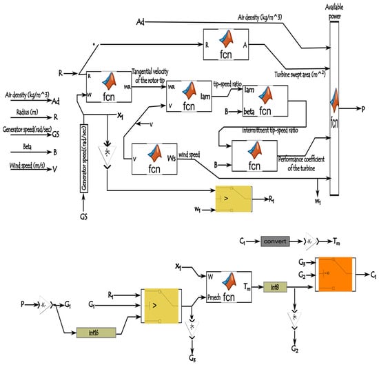
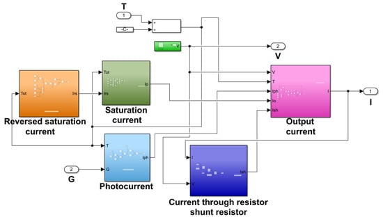
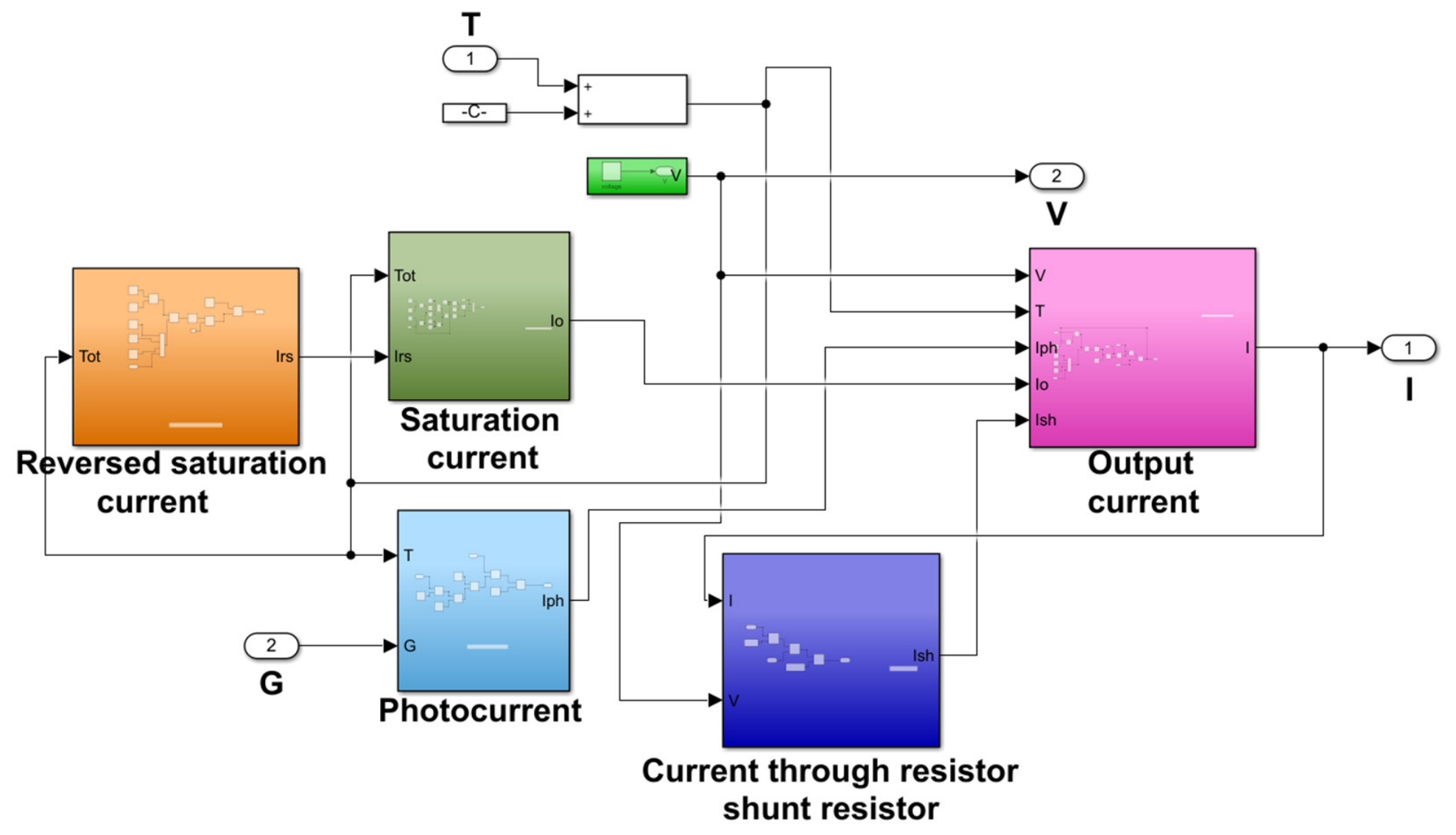
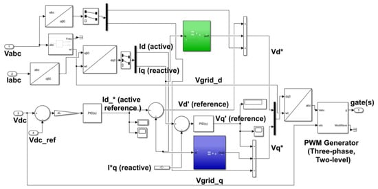
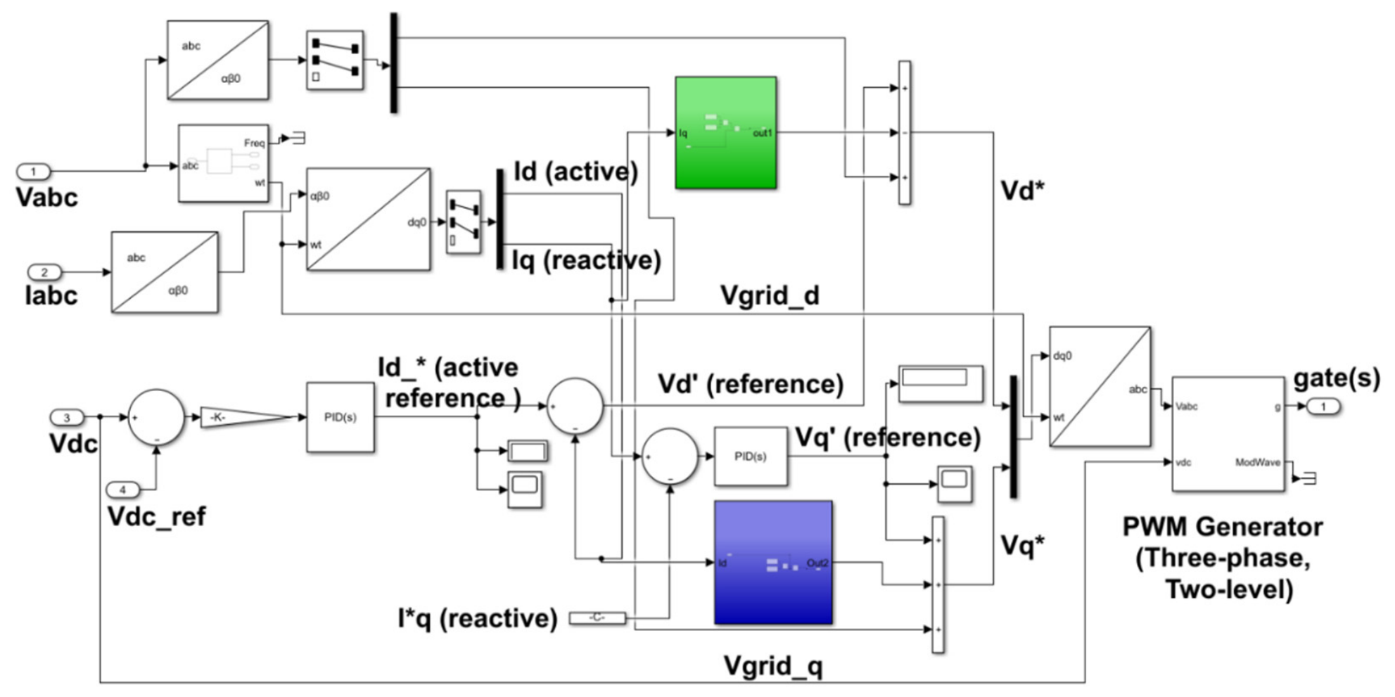
In this section, the hybrid multiterminal HVDC model contains referencing equations from this research to elucidate how they contribute to the overall efficiency of the system. Figure 2 shows the subsystem block of the wind turbine, and the Matlab function was used to execute the mathematical equations presented in Section 2.1, specifically Equations (1)–(5), which enhances the processing capabilities of the wind turbine by efficiently managing five distinct input parameters. The subsystem of Figure 3 represents the complete model of the photovoltaic solar system, as discussed in Section 2.2, specifically Equations (11)–(14). The photovoltaic system operates efficiently, optimally converting solar radiation into electrical energy that feeds into the HVDC network. Figure 4 details the inverter control model, which is necessary for regulating the operation of the three-phase inverter. The intricacies of the inverter control mechanism are thoroughly explored in Section 2.7, which described the modeling process conducted in Simulink. The model proved to maintain the system stability and efficiency. The topology of the entire system with respect to the circuit design is laid out in Figure 5.

Figure 2. Model of the wind turbine using the Matlab function.

Figure 3. Photovoltaic array model.

Figure 4. Inverter control model for the three-phase inverter.

Figure 5. Hybrid multiterminal HVDC network circuit.

5. Results and Discussions

The performance of the hybrid photovoltaic–wind energy conversion systems connected to an HVDC grid, along with the efficacy of the proposed control algorithms, has been assessed using the Matlab/Simulink simulation platform. Additionally, fault conditions, specifically DC line to ground fault, line to line fault at the rectifier end, and single line to ground fault at the inverter end with varying fault resistance values [13,49,50,51], were introduced at the receiving end with different fault locations, but with and without AC filters at the rectifier end will be considered to observe the behaviour generated. In this section, the detailed parameters are outlined in Table 1, and the simulation results for each scenario are presented.

Table 1. Hybrid multiterminal HVDC system parameters.

Parameters	Values	Unit
Wind energy conversion system
Mechanical power	3000	MW
Rated voltage	220	kV
Frequency	50	Hz
Pole(s)	6	-
Photovoltaic solar array
Power of the panel	750	W
Mechanical power	1000	MW
Series connected modules per string	28	-
Parallel strings	47,619	-
Open-circuit voltage	50.77	V
Short-circuit current	18.71	A
Current at maximum power point	17.58	A
Voltage at maximum power point	42.68	V
LC filter
Capacitance	5.581	µF
Inductance	18.16	mH
Three-phase transformer (two windings)
Nominal power	20	MVA
Resistance (p.u.)	0.0025	-
Leakage inductance (p.u.)	0.04	-
Magnetization resistance (p.u.)	500	-
Magnetization inductance(p.u.)	200	-
Distributed parameter transmission line (HVDC line)
Capacitance	0.0012	µF/km
Inductance	0.933	mH/km
Resistance	0.015	Ω/km
Cable length	1000	km
DC link voltage	1.464	kV
DC link current	1244	A
PID controller
Proportional	0	-
Integral	−1	-
Derivative	0	-
Filter coefficient	100	-

5.1. Without and with Filter During System Operation

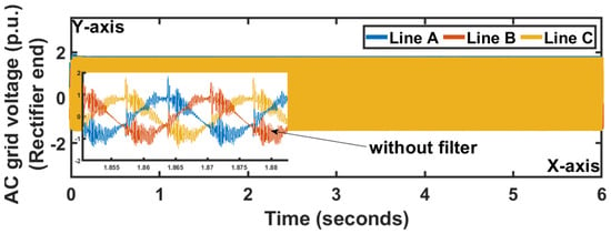
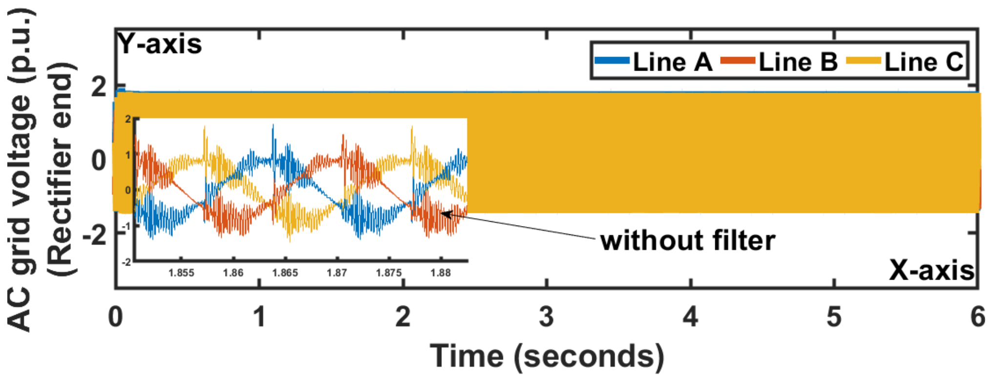
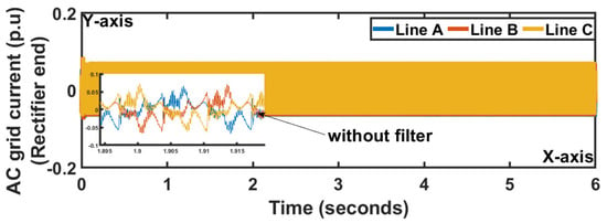
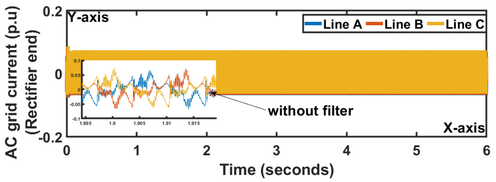
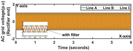
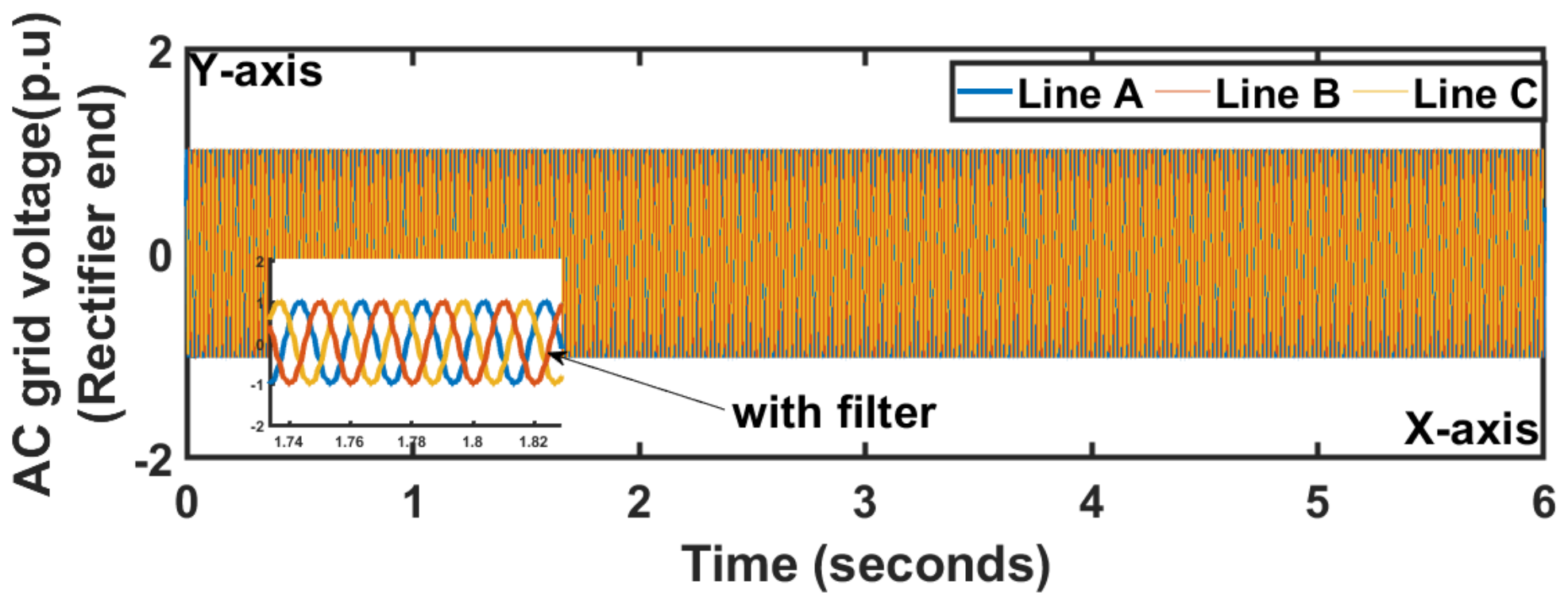
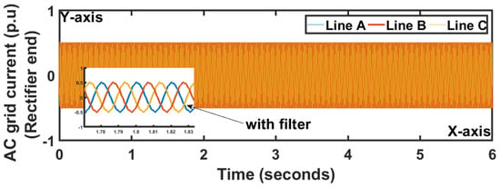
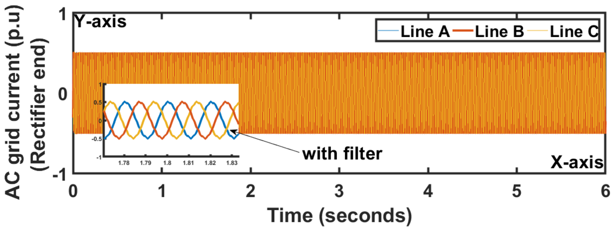
In the absence of AC filters during the operation of a hybrid multiterminal HVDC system, notable disturbances occur in the AC grid voltages and currents. This phenomenon is evident in the irregularities shown in Figure 6 and Figure 7, where divergence from a balanced sinusoidal waveform is observed. The absence of AC filters results in pollution within the AC grid, which leads to imbalances that will destabilize the system, and these irregularities in AC grid currents will produce a distorted waveform, typically characterized by an unbalanced sinusoidal shape, due to the switching actions of the rectifier bridge. However, the distortions will saturate transformer, which will cause excessive heating. Moreover, the instability exacerbated by these distortions will result in issues such as communication interference. In conjunction with the challenges presented by harmonic distortion, the operation of the HVDC link during the AC to DC conversion phase will bring critical concern: the potential for high surges in DC voltage and DC current at startup. In contrast, during the integration of AC filters on the rectifier side, the unwanted frequencies and waveform distortions will filter out, and their inclusion will allow for a more balanced sinusoidal waveform in both the AC grid voltages and currents shown in Figure 8 and Figure 9 by reducing the risk of system destabilization.

Figure 6. Result of AC grid voltages during the absence of AC filters at the rectifier end.

Figure 7. Outcomes of AC grid currents during the absence of AC filters at the rectifier end.

Figure 8. Simulation result of AC grid voltages with AC filters at the rectifier end.

Figure 9. Simulation outcomes of AC grid voltages with AC filters at the rectifier end.

5.2. DC Line to Ground Fault

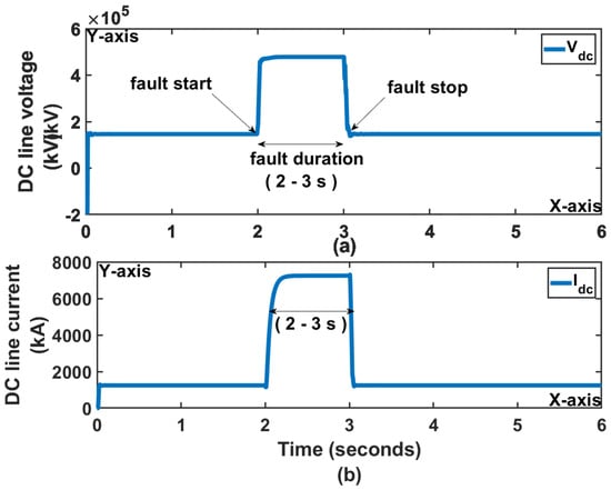
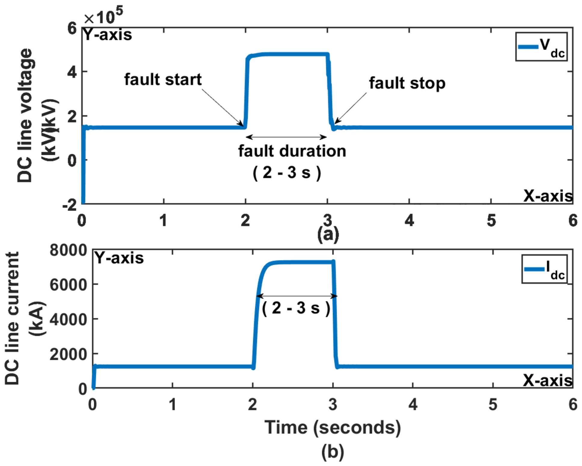
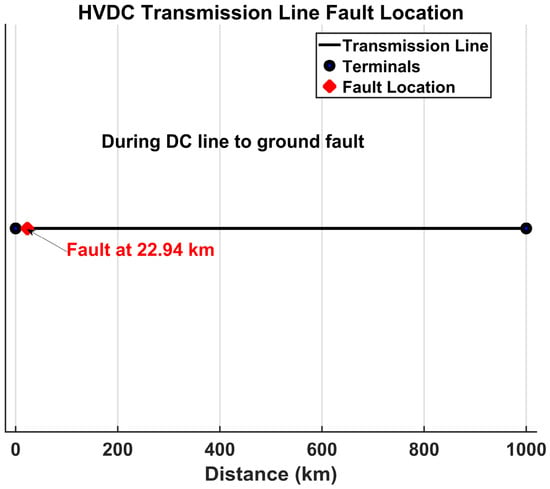
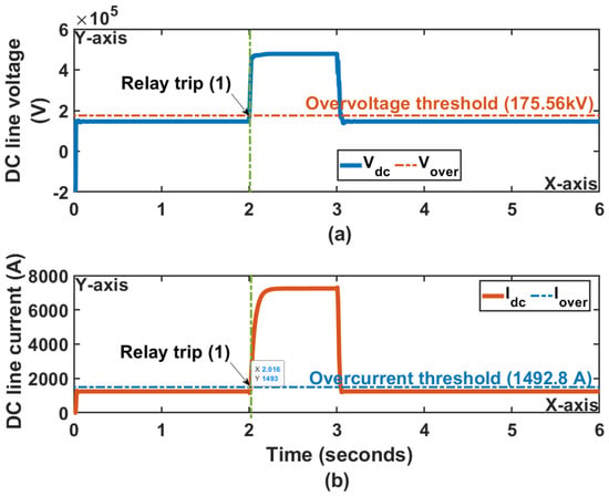
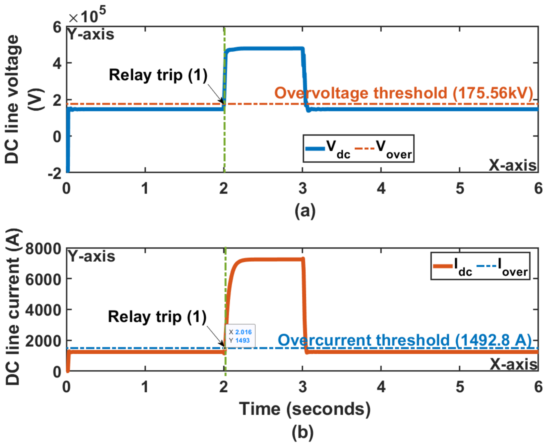
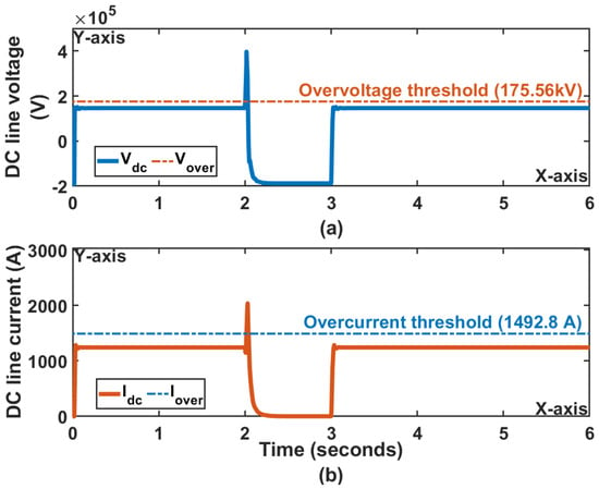
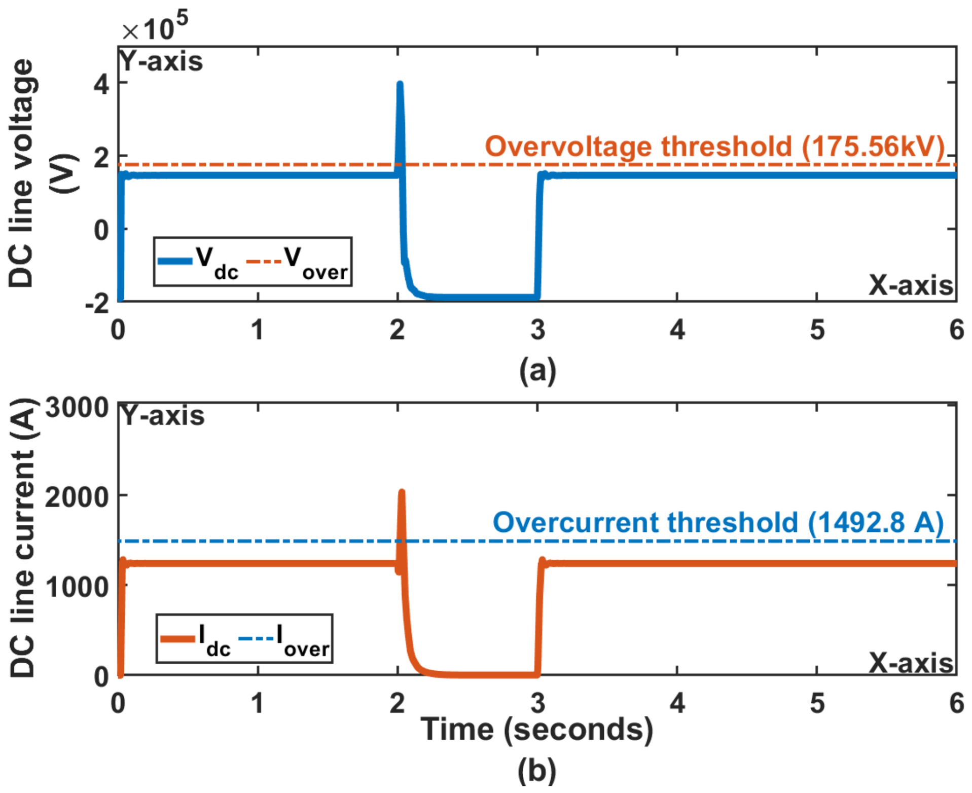
The initiation between 2.0 s and 3.0 s of the DC line to ground fault at 24 km on the HVDC line close to LCC rectifier station creates a sudden low-impedance path to the ground and generates steep voltage and current traveling waves that propagate fast along the transmission line, and the high rate of change of voltage of $102.64 \mathrm{V}/\mathrm{\mu }\mathrm{s}$ and rate of change of current of $0.137 \mathrm{A}/\mathrm{\mu }\mathrm{s}$ reflect influx of stored electrostatic and magnetic energy to collapse toward the ground point; the severe DC line voltage rise shown in Figure 10a and DC line current shown in Figure 10b increase shown in Table 2 result in a fault distance that is relatively short. Wave propagation delay is slightly infimum, enabling fast reflection of fault voltage and current that reach the threshold protection almost instantaneously after fault initiation at 2.0 s. At the rectifier and inverter ends, the AC grids react to the power imbalance reflected through the converter transformers. At the inverter side, power imbalance causes the AC grid voltages to rise with an overshoot as shown in Figure 11a. Meanwhile, the rectifier of AC grid voltages experiences increases as shown in Figure 12a and rises in rectifier AC grid currents, as shown in Figure 11b and Figure 12b, as the controls attempt to regulate real power flow against a DC line fault and the fault location on the HVDC line is shown in Figure 13. In addition, the overvoltage threshold is breached, as first shown in Figure 14a,b, triggering a breaker trip command, closely followed by an overcurrent trip at 2.016 s. The sudden spike observed right at these timestamps is shown in Figure 15a,b and corresponds to the reflection and refraction of electromagnetic waves at the boundary of opening DC circuit breaker contacts. In the end, fast tripping successfully isolates the line, preventing sustained thermal and dielectric damage to the converter stations. However, the recovery times across all metrics demonstrate effective clearance and stabilization by the system presented in Table 2.

Figure 10. (a) DC line voltage and (b) current during DC line to ground fault.

Table 2. Response of AC and DC parameters during DC line to ground fault.

System Location	Parameter	Pre-Fault Value	Fault Value	Peak Overshoot	Recovery Time
Inverter end	AC grid voltages	0.60 p.u.	0.75 p.u.	1.767 p.u.	3.08 s
Inverter end	AC grid currents	0.20 p.u.	0.25 p.u.	0.589 p.u.	3.08 s
Fault HVDC line	DC voltage	1.463 × 105 V	4.783 × 105 V	Transient state	3.24 s
Fault HVDC line	DC current	1244 A	7250 A	Transient state	3.24 s
Rectifier end	AC grid voltages	1.00 p.u.	1.20 p.u.	-	3.10 s
Rectifier end	AC grid currents	0.50 p.u.	0.65 p.u.	0.700 p.u.	3.10 s

Figure 11. (a) AC grid voltages and (b) AC grid currents at the inverter end during DC line to ground fault.

Figure 12. (a) AC grid voltages and (b) currents at the rectifier end during DC line to ground fault.

Figure 13. DC fault location during DC line to ground fault.

Figure 14. (a) Overvoltage at the DC voltage (b) overcurrent at the DC current during DC line to ground fault.

Figure 15. (a) DC voltage shutdown and (b) DC current shutdown during DC line to ground fault.

5.3. Single Line to Ground Fault at Inverter End

5.3.1. 8 Ohms

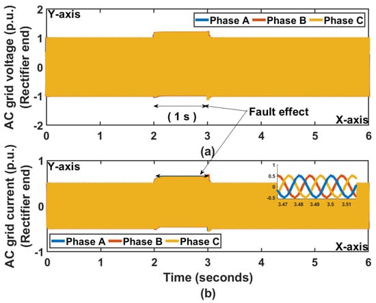
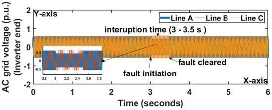
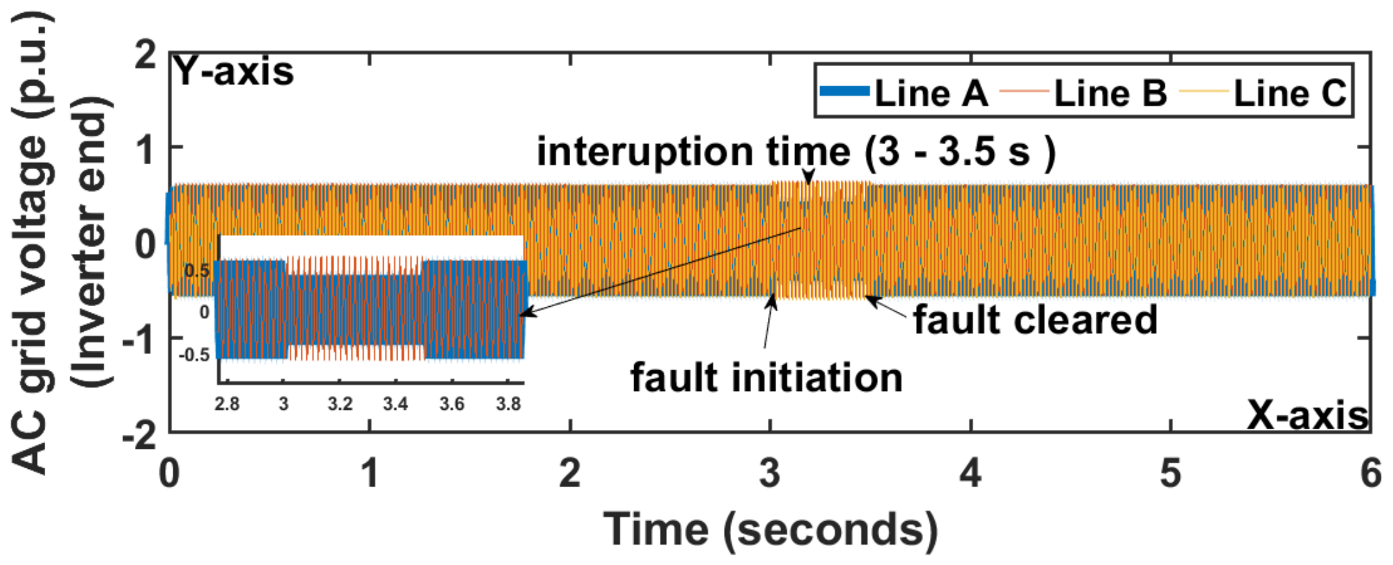
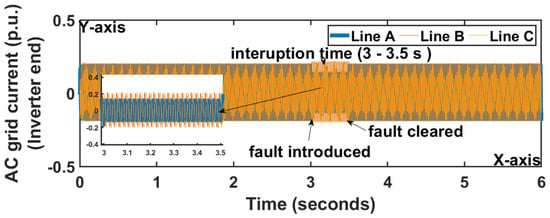
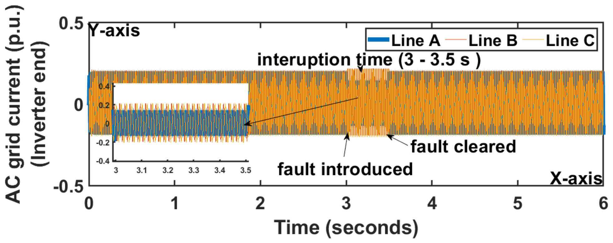
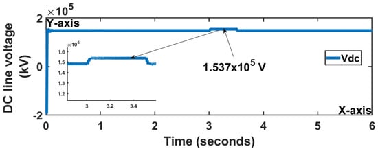
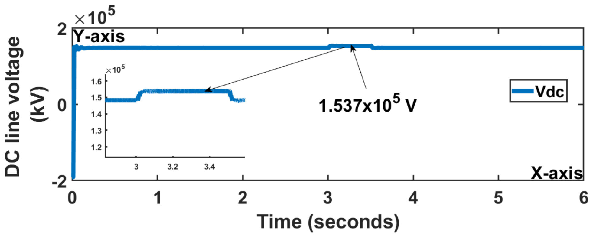
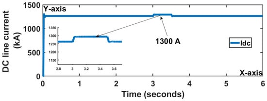
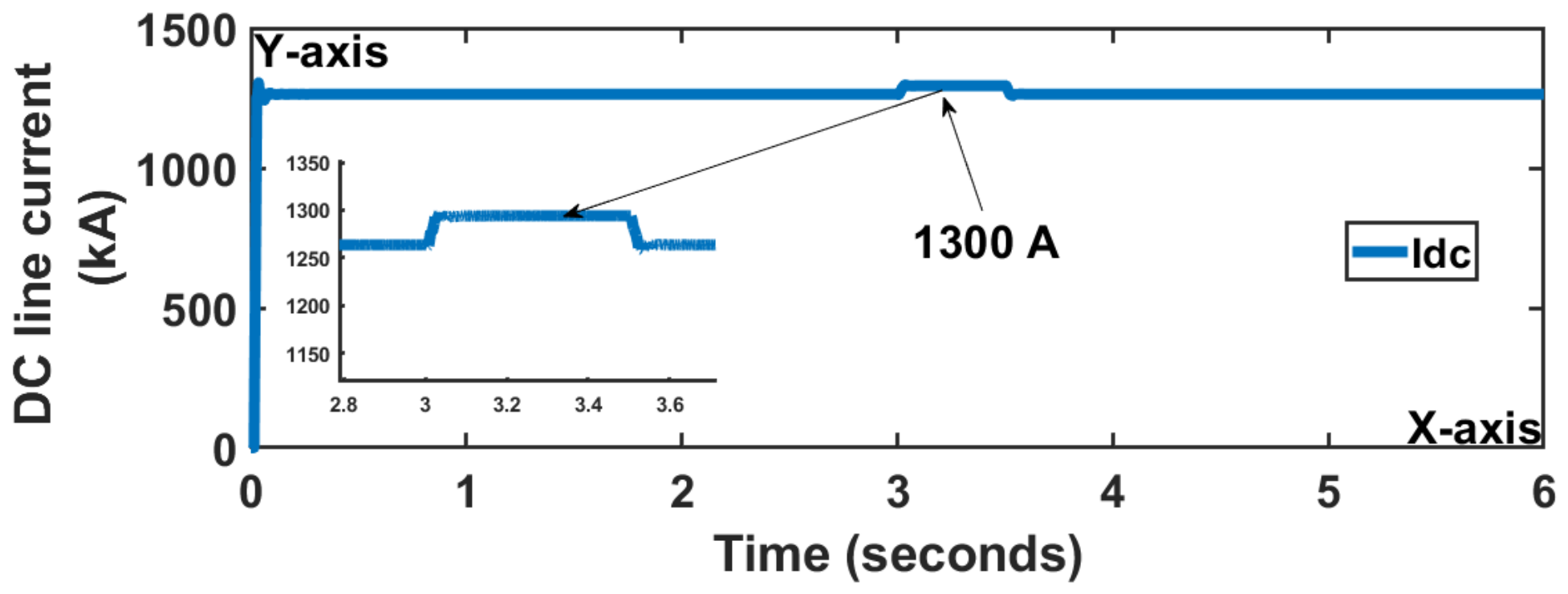
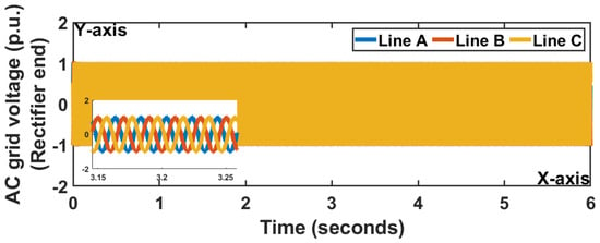
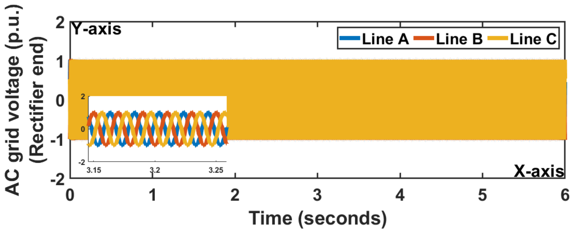
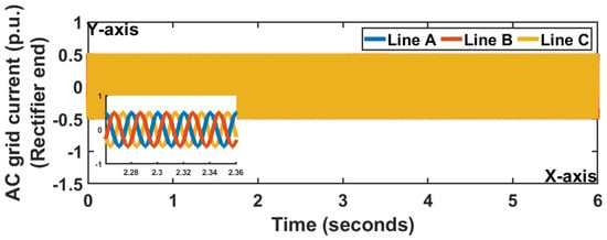
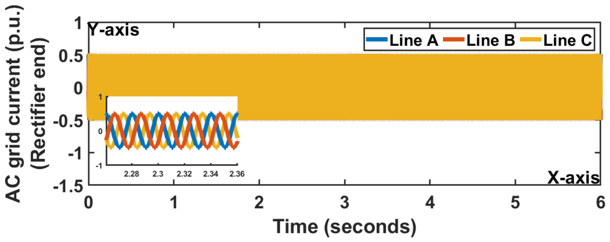
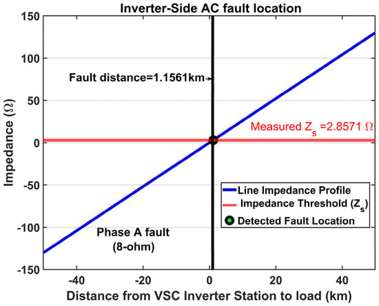
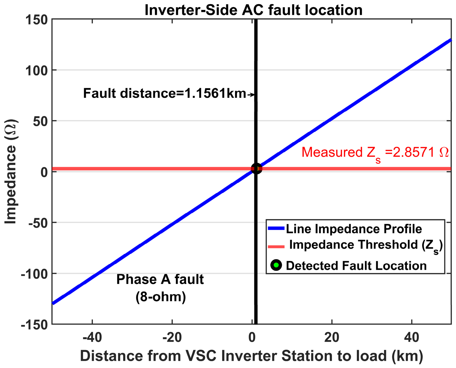
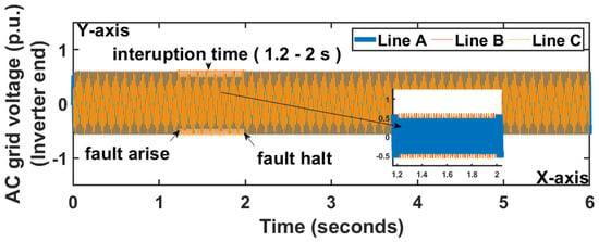
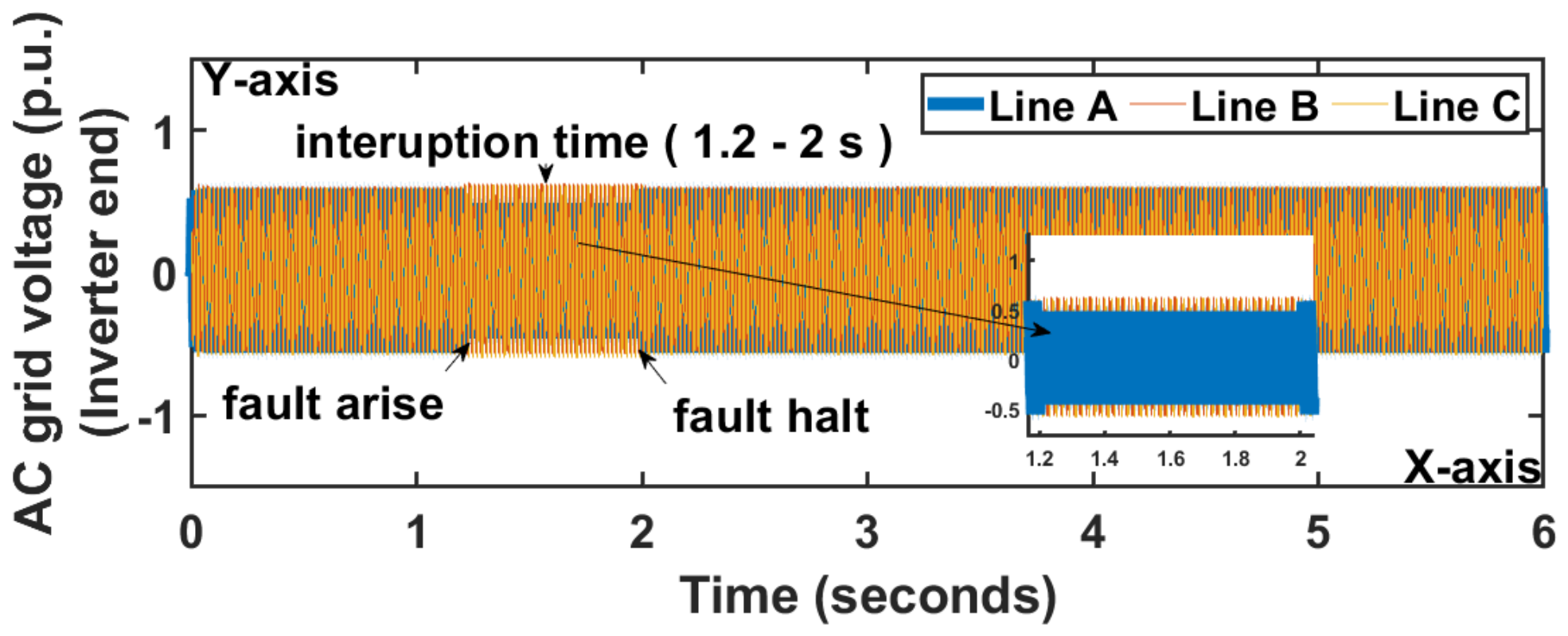
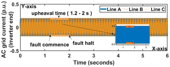
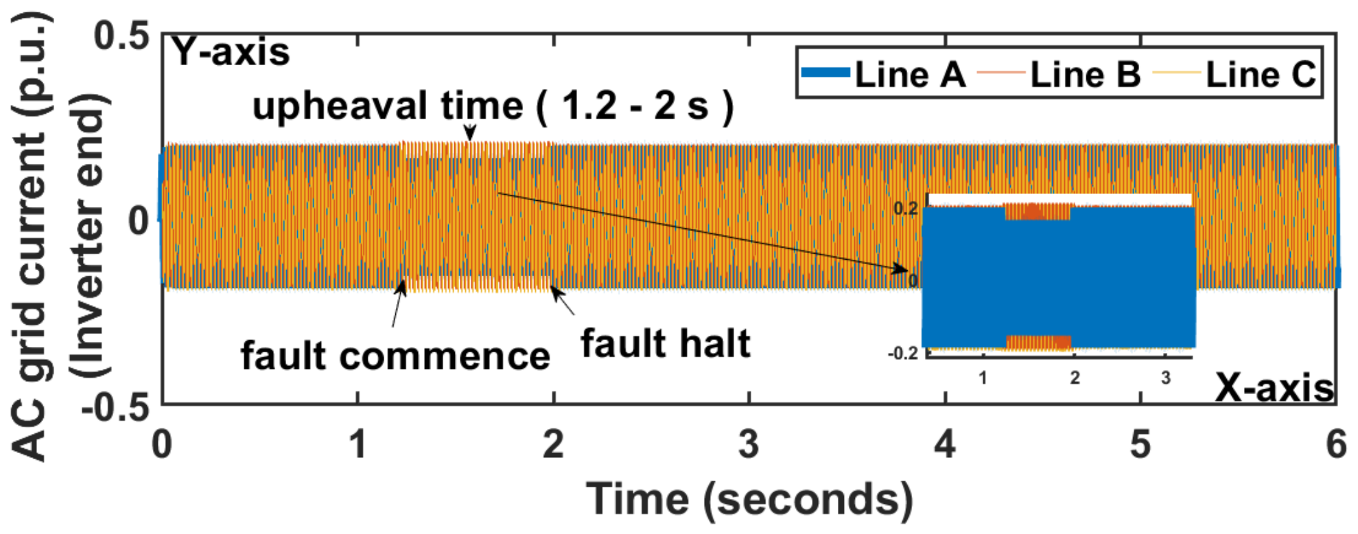
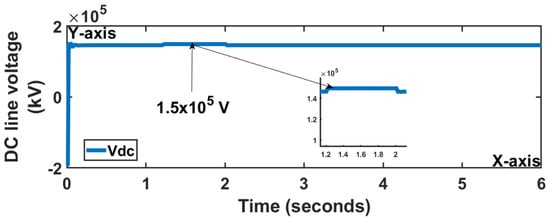
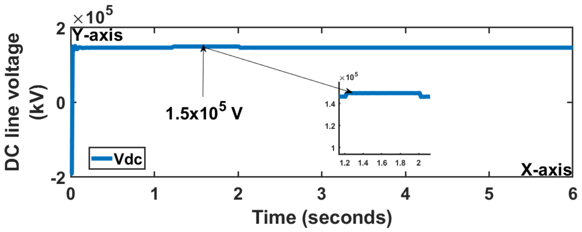
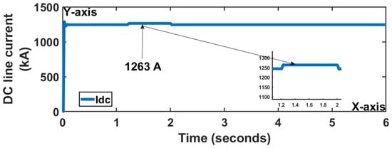
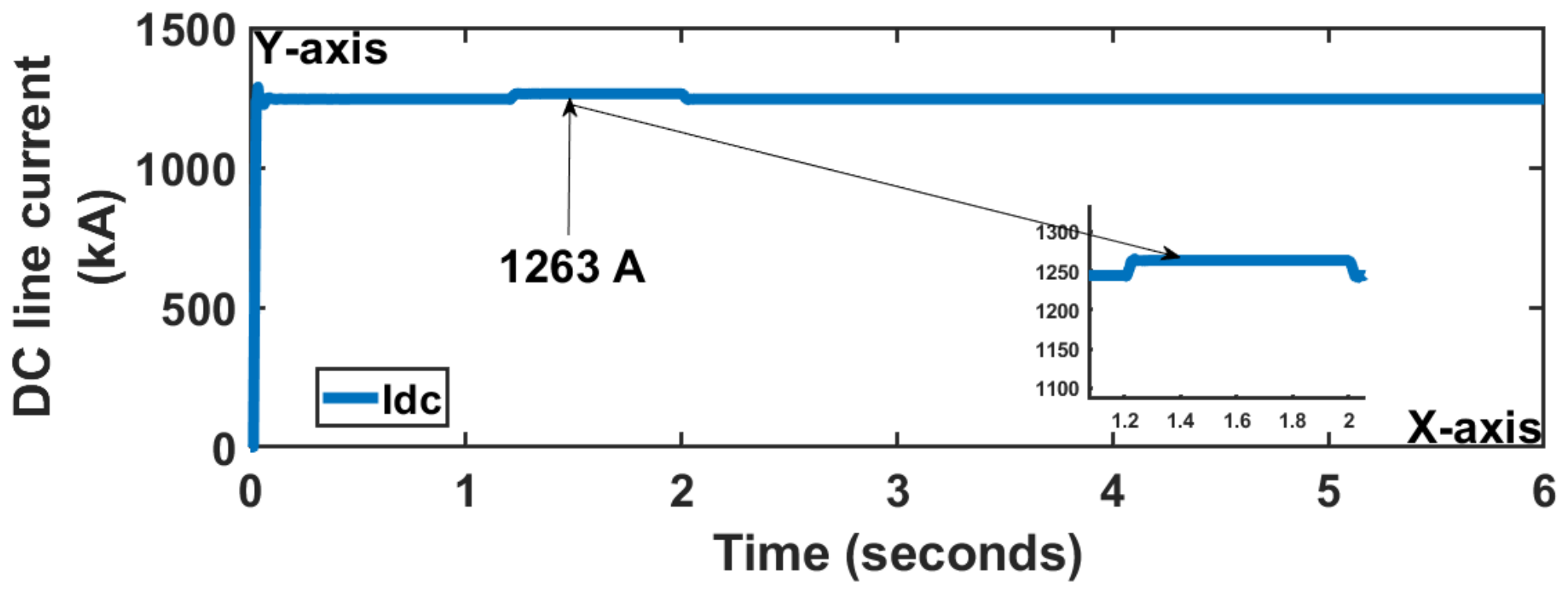
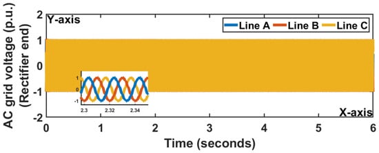
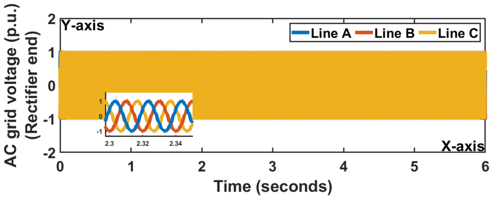
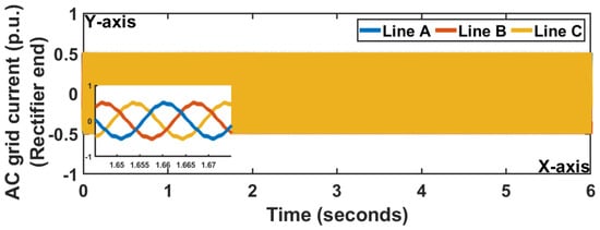
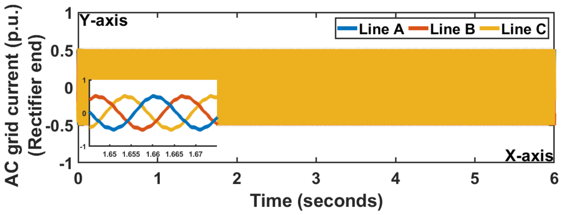
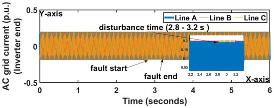
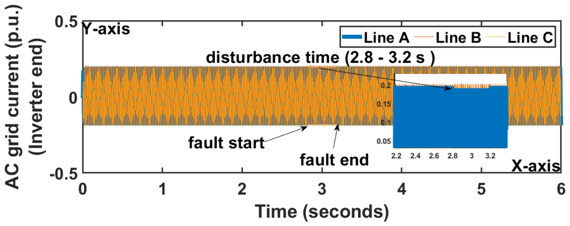
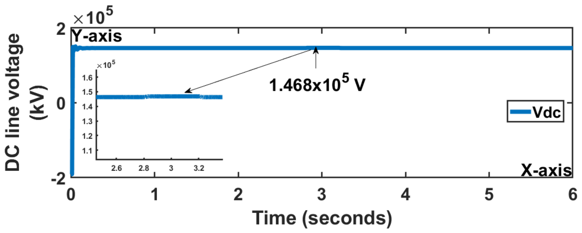
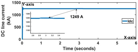
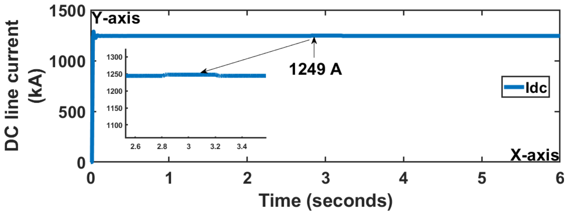
The system response during a single line to ground fault with 8-ohm fault resistance at the inverter end was evaluated. The fault was initiated between 3.0 s and 3.5 s, and the system response parameters are documented in Table 3. The inverter AC grid voltage sag and inverter AC grid current decreased on phase A at the inverter side are shown in Figure 16 and Figure 17, which reflect the impedance drop and energy imbalance caused by 8-ohm fault resistance. The rise in DC line voltage and DC line current shown in Figure 18 and Figure 19 indicates temporary HVDC link energy accumulation; the power injected by the rectifier side could not be fully transferred to the faulted inverter AC grid. The stable operation at the rectifier end of AC grid voltage and AC grid currents shown in Figure 20 and Figure 21 proves the high efficacy of the single tuned filter and capacitor filter. These filters successfully isolated the rectifier station from severe transient propagation, verifying that filtering prevents cascading failures across extended HVDC links. However, the calculated fault distance shown in Figure 22 within the 2 km AC line validates the precision of the parameters, and after the fault initiation, the system recovers by the value given in Table 3 to the nominal operating conditions.

Table 3. System response parameters during 8 ohms under single line to ground fault.

System Location	Parameter	Pre-Fault Value	Fault Value	Peak Overshoot	Recovery Time
Fault inverter end	AC grid voltage (phase A)	0.60 p.u.	0.4 p.u.	Unhealthy state	3.55 s
	AC grid current (phase A)	0.20 p.u.	0.14 p.u.	Unstable state	3.55 s
HVDC line	DC voltage	1.463 × 105 V	1.537 × 105 V	Transient	3.58 s
	DC current	1244 A	1300 A	Transient	3.57 s
Rectifier end	AC grid voltages	1.00 p.u.	1.00 p.u.	Stable state	Unaffected
	AC grid currents	0.50 p.u.	0.5 p.u.	Stable state	Unaffected

Figure 16. Result of AC grid voltages during 8 ohms of resistance under single line to ground fault at the inverter end.

Figure 17. Outcome of grid currents during 8 ohms of resistance under single line to ground fault at the inverter end.

Figure 18. DC voltage results during 8 ohms of resistance under single line to ground fault that occurred at the inverter end.

Figure 19. DC current outcomes during 8 ohms of resistance under single line to ground fault that occurred at the inverter end.

Figure 20. Result of AC grid voltages at the rectifier end during 8 ohms of resistance under single line to ground fault that occurred at the inverter end.

Figure 21. AC grid currents at the rectifier end during 8 ohms of resistance under single line to ground fault that occurred at the inverter end.

Figure 22. Fault location at the inverter end during 8 ohms of resistance under single line to ground fault that occurred at the inverter end.

5.3.2. 15 Ohms

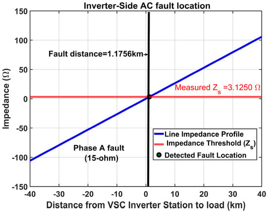
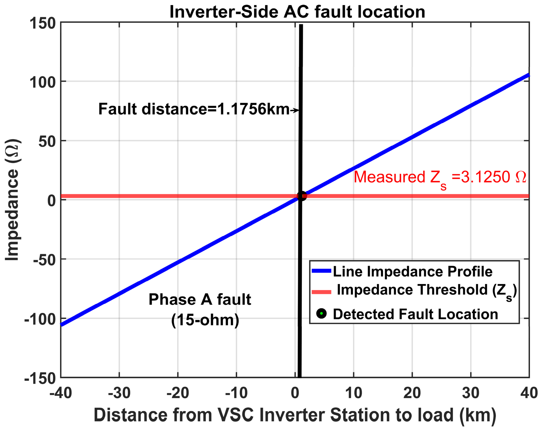
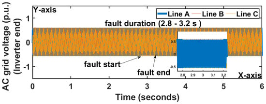
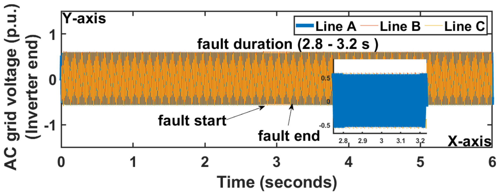
The behavior of the system during the single line to ground fault with 15-ohm resistance reveals the voltage source and the effectiveness of the system’s filtering topology. As presented in Table 4, the performance of the system during 15 ohms under single to ground fault demonstrated the efficacy of the control and the filtering strategies. The sudden drop in the inverter AC grid voltage of phase A shown in Figure 23 reflects the impedance divider effect created by the 15-ohm fault resistance, because the fault occurred at the distance on a 2 km line; the remaining short line segment limited the severity of the AC grid voltage while the inverter AC grid current drop is as shown in Figure 24, with different recovering stages documented in Table 4. The rise in DC line voltage and current shown in Figure 25 and Figure 26 occur due to an active power imbalance. When the inverter AC system end experiences a fault with a fault resistance value, it cannot export active power into the grid at the same rate that the rectifier end injects it from the source. This transient power mismatch charges the DC link capacitor, raising the DC voltage until it is cleared. However, recovery occurs rapidly as shown in Table 4 once the fault is cleared and power equilibrium is restored. The rectifier end maintains a baseline as shown in Figure 27 of an AC grid voltage profile because the DC line decouples AC dynamics on one side from the other. Furthermore, single-tuned and capacitor bank filters absorb high-frequency harmonic ripples. The stable AC grid current performance of healthy phases (B and C) shown in Figure 28 underscores balanced structural immunity against cross-phase propagation and fault location on the inverter end is shown in Figure 29. However, Table 4 shows the state before, during, and after fault recovery.

Table 4. System response parameters during 15-ohm resistance under single line to ground fault.

System Location	Parameter	Pre-Fault Value	Fault Value	Peak Overshoot	Recovery Time
Fault Inverter end	AC grid voltage (phase A)	0.60 p.u.	0.5 p.u.	Unbalanced state	2.20 s
	AC grid current (phase A)	0.20 p.u.	0.16 p.u.	Unbalanced state	2.22 s
HVDC line	DC voltage	1.464 × 105 V	1.5 × 105 V	Transient state	2.10 s
	DC current	1244 A	1263 A	Transient state	2.11 s
Rectifier end	AC grid voltages	1.00 p.u.	1.00 p.u.	Stable state	Unaffected
	AC grid currents	0.50 p.u.	0.5 p.u.	Stable state	Unaffected
Fault location	Fault distance from VSC inverter to load	2 km	1.1756 km	-	-

Figure 23. Grid voltages during 15 ohms of resistance under single line to ground fault at the inverter end.

Figure 24. Grid currents during 15 ohms of resistance under single line to ground fault at the inverter end.

Figure 25. DC voltage during 15 ohms of resistance under single line to ground fault that occurred at the inverter end.

Figure 26. DC current during 15 ohms of resistance under single line to ground fault that occurred at the inverter end.

Figure 27. Grid voltages at the rectifier end during 15 ohms of resistance under single line to ground fault that occurred at the inverter end.

Figure 28. Grid currents at the rectifier end during 15 ohms of resistance under single line to ground fault that occurred at the inverter end.

Figure 29. Fault location at the inverter end during 15 ohms of resistance under single line to ground fault that occurred at the inverter end.

5.3.3. 100 Ohms

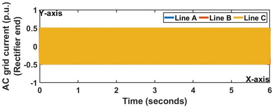
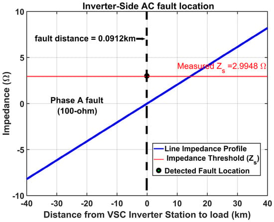
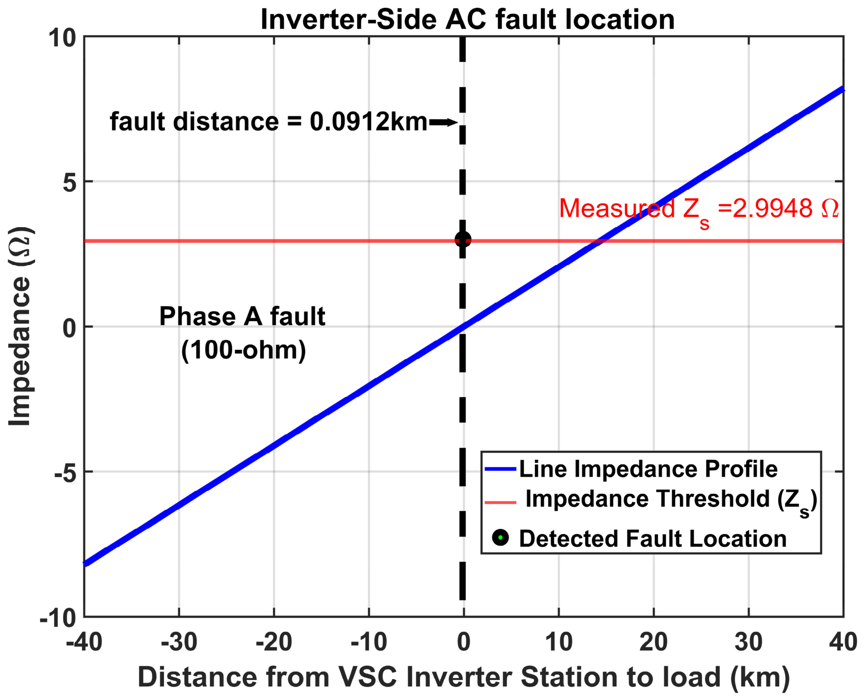
The mechanisms governing the observed responses involve instantaneous power imbalances and the propagation of electromagnetic waves through the transmission network. The drop in inverter AC grid voltage in Table 5 and the behavior shown in Figure 30 result directly from the sudden 100-ohm fault resistance path at a distance, and this creates an immediate voltage divider effect between the system source impedance and the fault impedance. The decline in the inverter AC grid current shown in Figure 31 aligns with Ohm’s law, and the lower inverter AC grid voltage driving the load yields a proportional reduction in current draw during the fault scenario. The instability preceding recovery of inverter AC grid voltage shown in Table 5 matches the electromechanical and control loop readjustments of the VSC controller as they restore phase-lock loop (PLL) synchronization and nominal AC grid references. The simultaneous rise in DC voltage and DC current, as shown in Table 5, and their behaviors, as shown in Figure 32 and Figure 33, indicate an instantaneous active power surplus on the DC link due to the inverter AC grid side fault restricting power evacuation from the inverter station to the grid and the continuous kinetic from the rectifier side temporarily accumulating in the DC link capacitors; this elevates the DC capacitor stored energy and yields a temporary voltage and current rise until the inverter control successfully rebalances the power flow at given value, as shown in Table 5. Furthermore, the constancy of the rectifier AC grid voltages and rectifier AC grid currents presented in Table 5 and the behavior shown in Figure 34 and Figure 35 mirrors the decoupling capability of DC line storage coupled with effective AC filtering at the rectifier end. The use of the single-tuned filter and capacitor bank at the rectifier terminal successfully shunts high-frequency switching and transient ripple but prevents backward propagation of the inverter side fault disturbances across the HVDC line and the fault location at the inverter end of the AC system is shown in Figure 36.

Table 5. System response parameters during 100 ohms of resistance under single line to ground fault.

System Location	Parameter	Pre-Fault Value	Fault Value	Peak Overshoot	Recovery Time
Fault Inverter end	AC grid voltage (phase A)	0.60 p.u.	0.5 p.u.	Unbalanced state	3.4 s
	AC grid current (phase A)	0.20 p.u.	0.16 p.u.	Unbalanced state	3.41 s
HVDC line	DC voltage	1.464 × 105 V	1.468 × 105 V	Transient state	3.45 s
	DC current	1244 A	1249 A	Transient state	3.46 s
Rectifier end	AC grid voltages	1.00 p.u.	1.00 p.u.	Stable state	Unaffected
	AC grid currents	0.50 p.u.	0.5 p.u.	Stable state	Unaffected
Fault location	Fault distance from VSC inverter to load	2 km	0.0912 km	-	-

Figure 30. Outcome of grid voltages during 100 ohms of resistance under single line to ground fault at the inverter end.

Figure 31. Result of grid currents during 100 ohms of resistance under single line to ground fault at the inverter end.

Figure 32. DC voltage outcome during 100 ohms of resistance under single line to ground fault that occurred at the inverter end.

Figure 33. DC current result during 100 ohms of resistance under single line to ground fault that occurred at the inverter end.

Figure 34. Outcome of grid voltages at the rectifier end during 100 ohms of resistance under single line to ground fault that occurred at the inverter end.

Figure 35. Result of grid currents at the rectifier end during 100 ohms of resistance under single line to ground fault that occurred at the inverter end.

Figure 36. Fault location at the inverter end during the 100 ohms of resistance under single line to ground fault that occurred at the inverter end.

5.4. Line to Line Fault

5.4.1. 0.001 Ohms

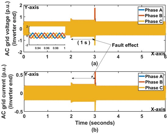
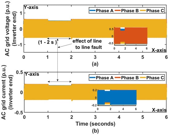
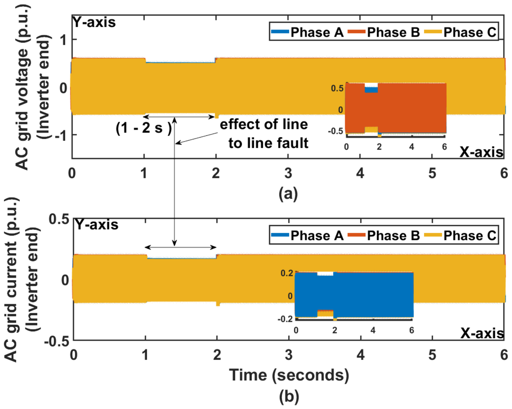
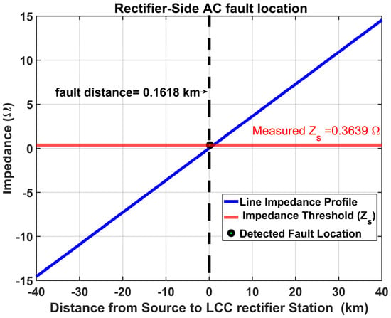
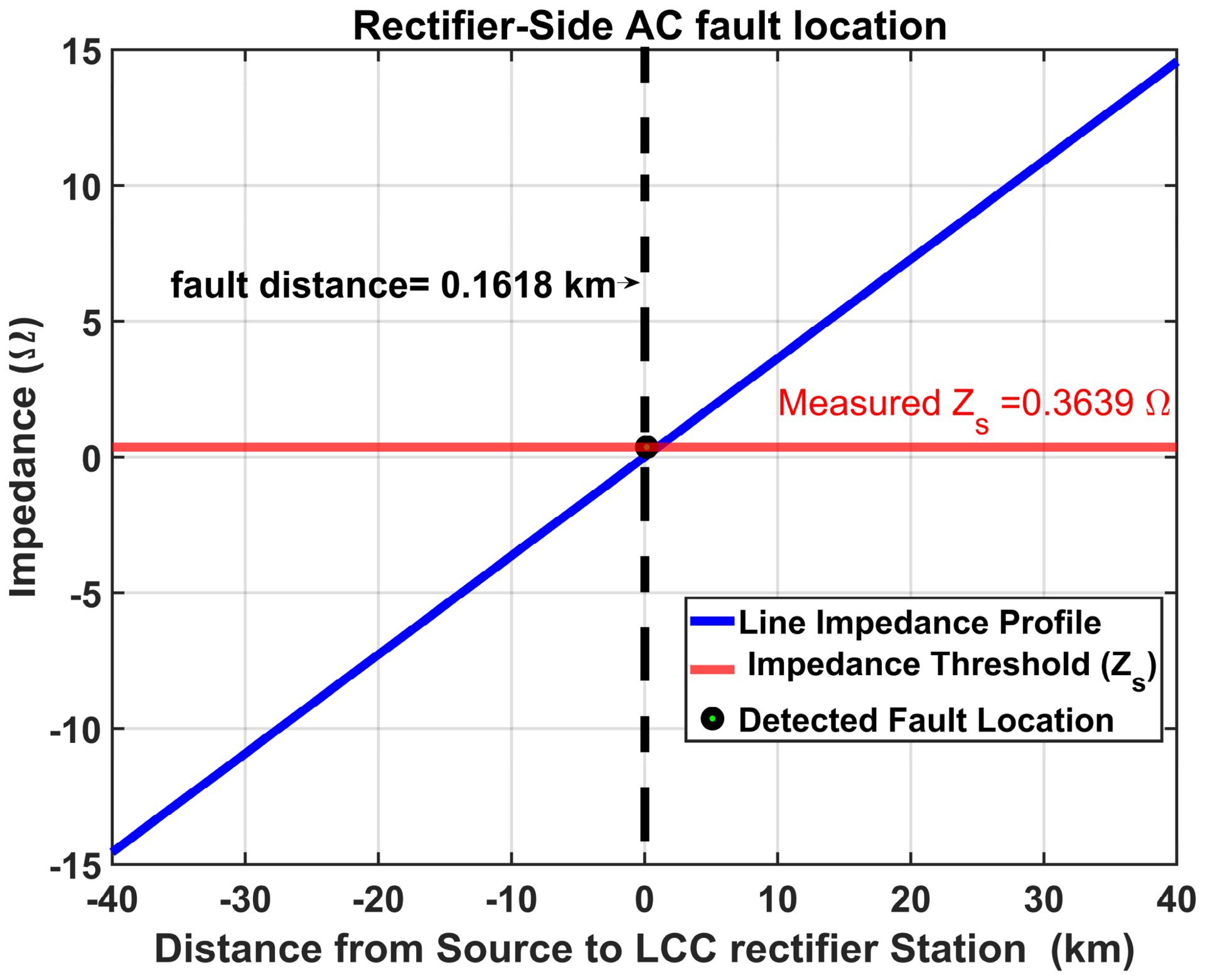
The collapse of the AC grid voltage of phase A shown in Figure 37a reflects a line to line fault situated close to the source station, and the fault impedance is low with a short-circuit current path created, pulling the faulted phase AC grid voltage down completely. The rectifier AC grid currents rise as shown in Figure 37b, which aligns with the low-impedance boundary condition. The single tuned and capacitor bank filters effectively mitigated harmonic distortion to maintain a steady waveform, yet they could not prevent the initial current overshoot of 1.008 s, as shown in Figure 37b, but mitigate higher-order harmonics, as seen in the recovery envelopes once the fault is cleared. At the HVDC line, the DC line voltage drops, which directly follows the rectifier AC grid voltage fault at the LCC rectifier bridge, which reduces the DC line converted output voltage shown in Figure 38a. The dip in DC line current as shown in Figure 38b at fault inception corresponds to the discharge phase of inductor-capacitor elements before the controls adjust. The overshoots for DC line voltage and DC line current upon fault clearance represent magnetic and electrostatic energy rebounds as the system inductances and AC filter banks re-energize during the transient recovery state. At the inverter side, displays of distinct phase by phase asymmetry of different values of AC grid voltages and AC grid currents are shown in Figure 39a,b. This imbalance is a characteristic of an unhealthy line to line fault propagation through transformer coupling configurations of a line-commutated converter system and the DC link to VSC inverter station. The inverter AC grid currents sag to lower fault state magnitudes, as shown in Figure 39b, and downward overshoot dip during recovery at the inverter AC grid voltages. The fault location at the rectifier end of an AC system is shown in Figure 40. However, the system parameters before, during, and after the fault recovery are summarized in Table 6.

Figure 37. (a) AC grid voltages and (b) AC grid currents at the rectifier end during 0.001 ohms of resistance under line to line fault at the rectifier side.

Figure 38. (a) DC line voltage and (b) current during 0.001 ohms of resistance under line to line fault at the rectifier end.

Figure 39. (a) AC grid voltages and (b) AC grid currents at the inverter end during 0.001 ohms of resistance under line to line fault at rectifier side.

Figure 40. Fault location at the rectifier end during 0.001 ohms of resistance under line to line fault that occurred at the rectifier end.

Table 6. System response parameters during 0.001-ohm under line-to-line fault.

Parameter	Pre-Fault Value	Fault Value	Post-Clearing Overshoot	Recovery Time (s)
Rectifier AC voltage (phase A)	1.0 p.u.	0.0 p.u.	1.2 p.u.	2.06
Rectifier AC voltage (phase B)	1.0 p.u.	0.91 p.u.	-	2.06
Rectifier AC current (A/B)	0.5 p.u.	2.5 p.u.	-	2.05
HVDC line voltage	1.464 × 105 V	8.4 × 104 V	2.0 × 105 V	2.18
HVDC line current	1244 A	975 A (dip)/1115 A	1350 A	2.172
Inverter AC voltage(A/B/C)	0.6 p.u.	0.488 p.u.	-	2.05
		0.456 p.u.	-
		0.482 p.u.	0.52 p.u. (dip)
Inverter AC current (A/B/C)	0.2 p.u.	0.13 p.u.		2.1
		0.1675 p.u.
		0.172 p.u.

5.4.2. 8 Ohms

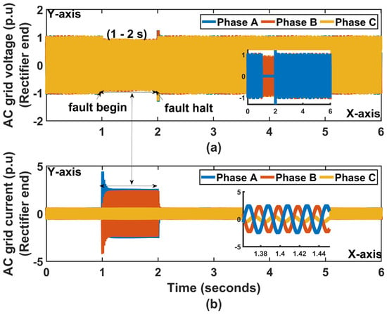
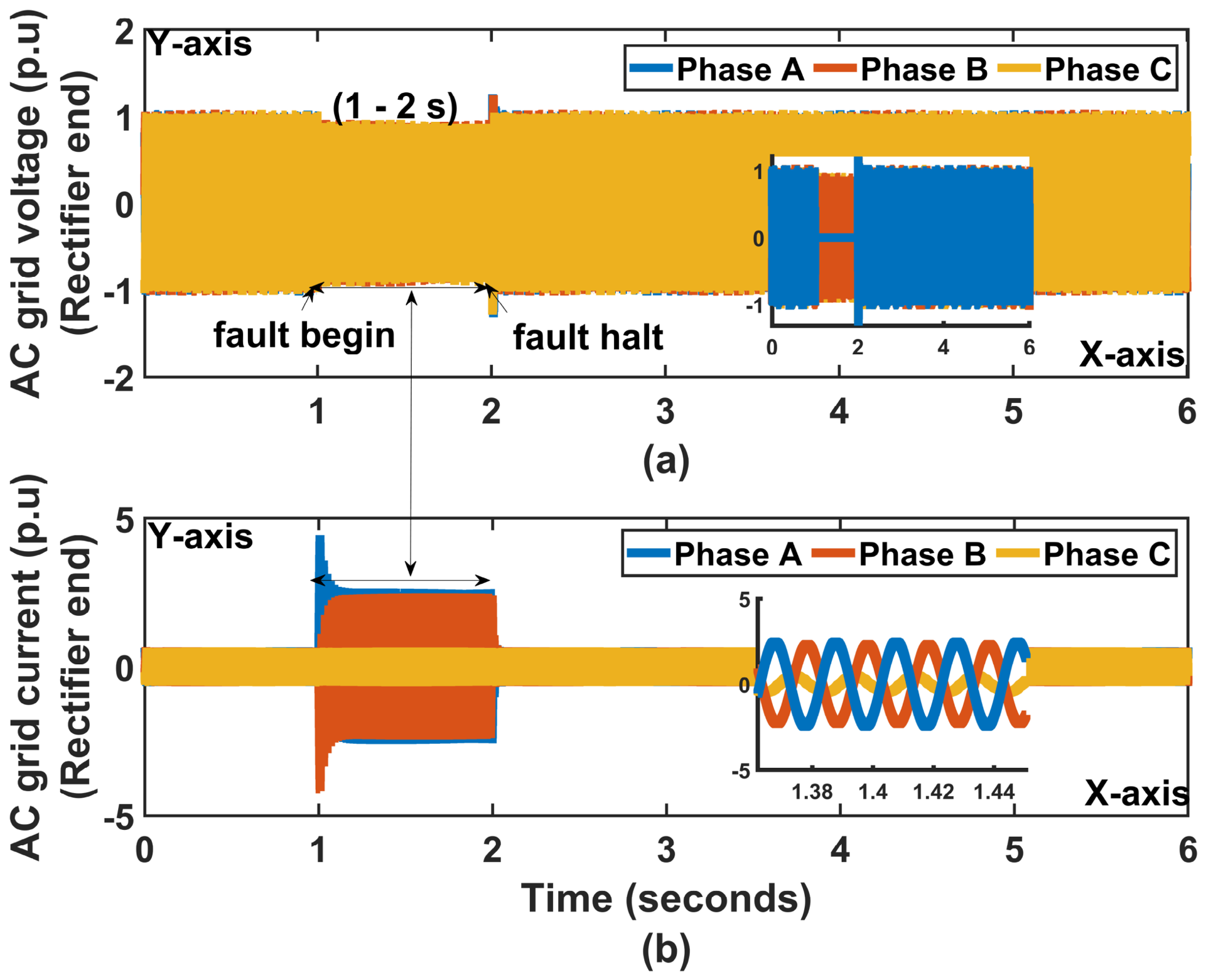
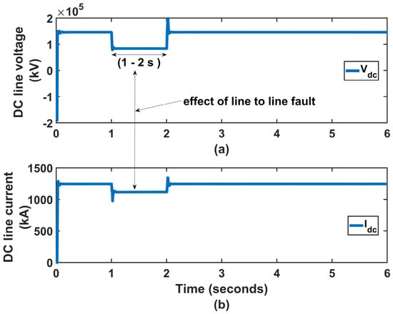
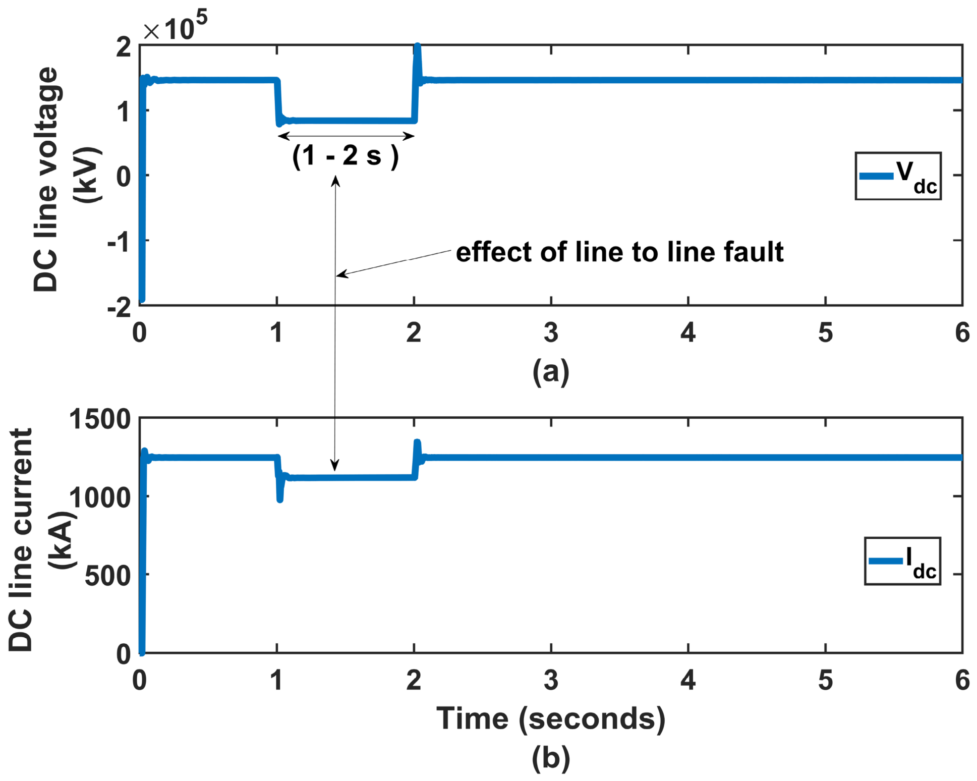
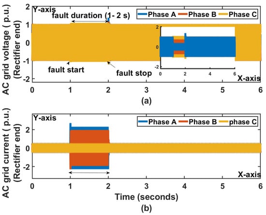
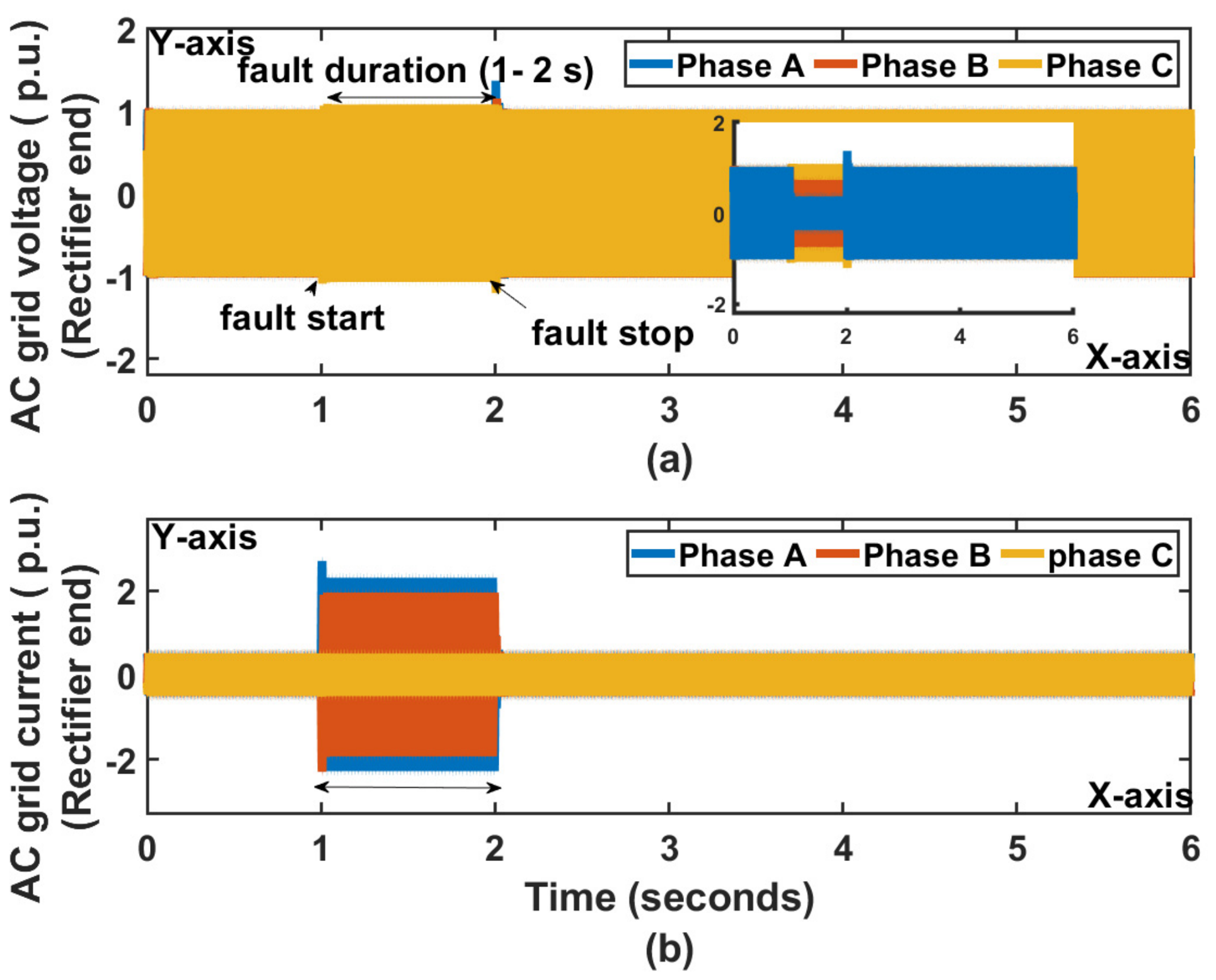
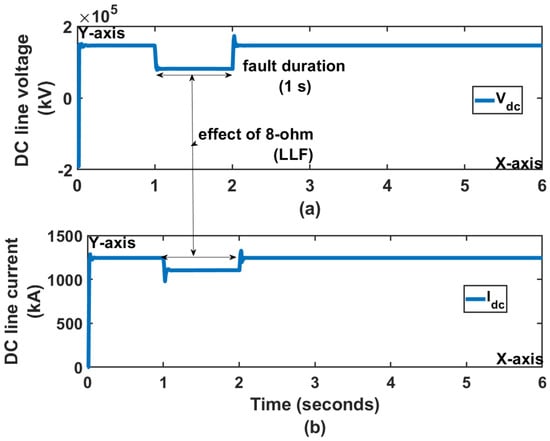
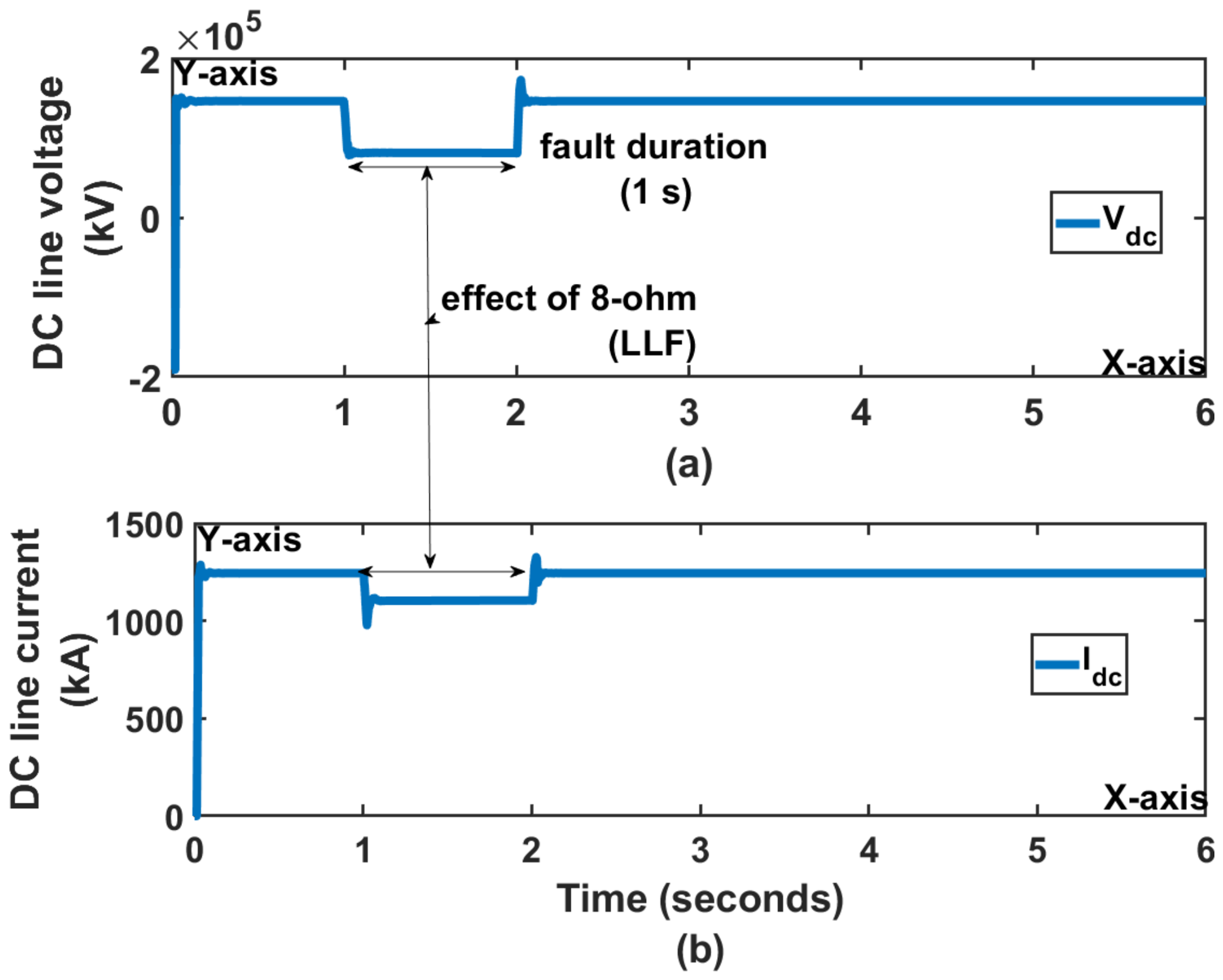
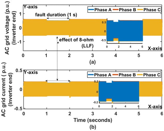
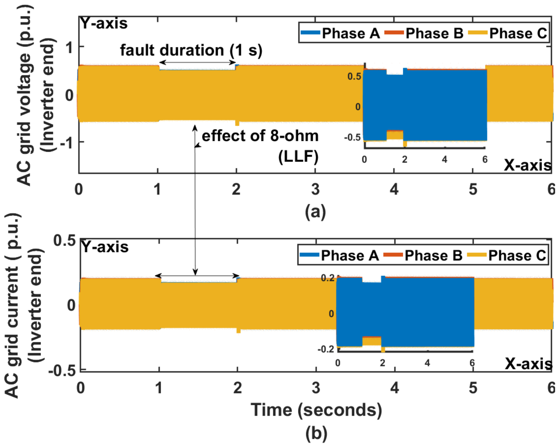
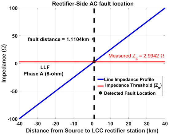
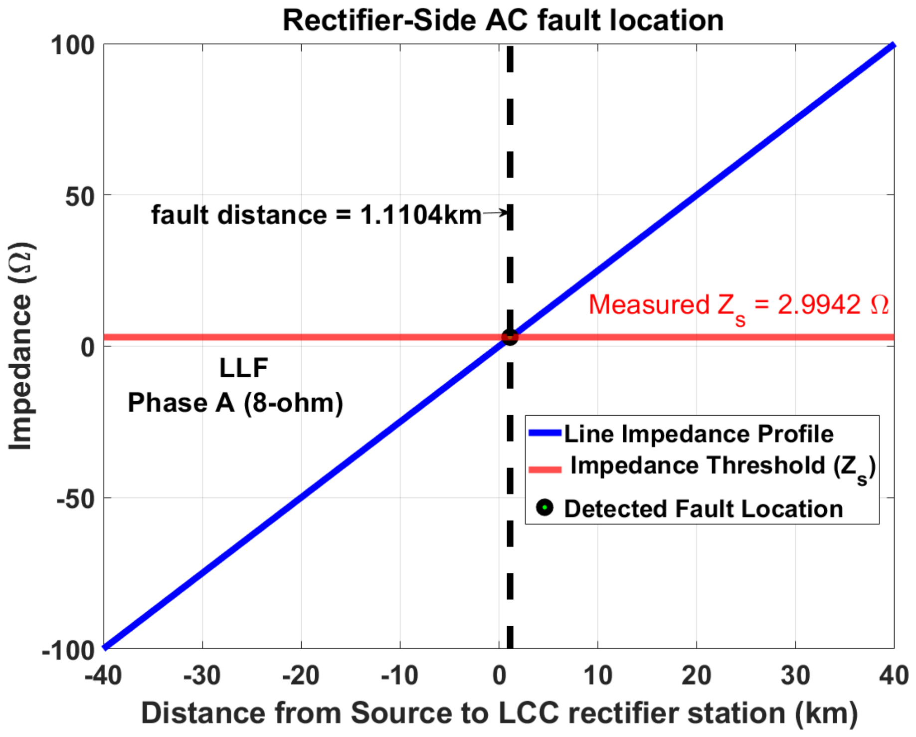
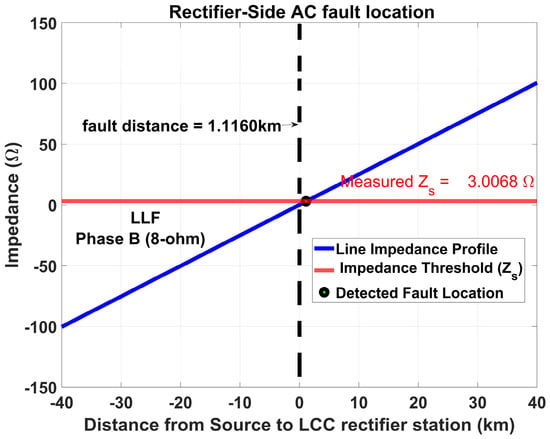
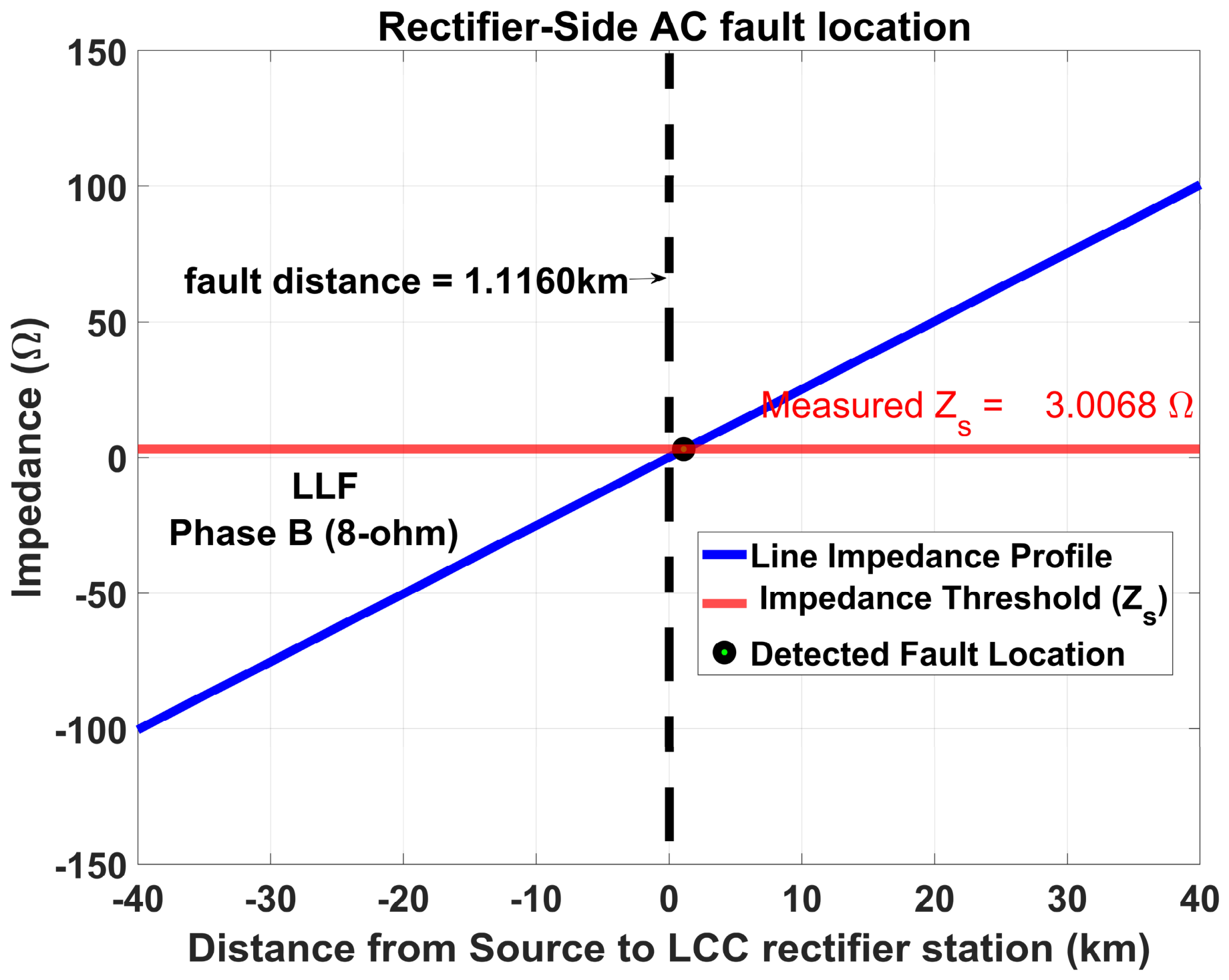
The asymmetrical rectifier AC grid voltage drop, and rectifier AC grid current surge shown in Figure 41a,b during the 8-ohm line-to-line fault reflects the low impedance path. The decrease in phase A at the rectifier end of AC grid voltage compared with phase B of AC grid voltage indicated higher angular involvement of the AC grid voltage of phase A to the initial point. The single tuned and capacitor bank filters effectively mitigated harmonic distortion during the active fault period. The DC voltage surge alongside the dip and surge in DC line current shown in Figure 42a,b, showing that the adjustment of LCC firing angles and DC reactance tried to stabilize active power transfer during the unsymmetrical AC grid disturbance. Regarding recovery, clustered between the recorded time presented in Table 7, the system restored successfully. At the inverter end, the uniform reduction of AC grid voltages and AC grid currents shown in Figure 43a,b reflect the wave propagation delay and attenuation across the transmission line impedance due to the VSC inverter under depressed DC link voltage. Furthermore, the estimated fault locations shown in Figure 44 and Figure 45 closely align with one another. This slight discrepancy between phases is physically attributed to measurement noise PI section line variations and transient wave reflection timings. However, the system parameters before, during, and after the fault recovery are summarized in Table 7.

Figure 41. (a) AC grid voltages and (b) AC grid currents at the rectifier end during 8 ohms of resistance under line to line fault at rectifier side.

Figure 42. (a) DC line voltage and (b) current during 8 ohms of resistance under line to line fault at the rectifier end.

Table 7. System response parameters during 8 ohms of resistance under line-to-line fault.

Parameter	Pre-Fault Value	Fault Value	Post-Clearing Overshoot	Recovery Time (s)
Rectifier AC voltage (phase A)	1.0 p.u.	0.368 p.u.	1.2 p.u.	2.08
Rectifier AC voltage (phase B)	1.0 p.u.	0.735 p.u.	-	2.08
Rectifier AC current (phase A)	0.5 p.u.	2.300 p.u.	-	2.08
Rectifier AC current (phase B)	0.5 p.u.	1.950 p.u.		2.08
HVDC line voltage	1.464 × 105 V	8.126 × 104 V	1.728 × 105 V	2.20
HVDC line current	1244 A	980 A (dip)/1100 A	1326 A	2.15
Inverter AC voltage(A/B/C)	0.6 p.u.	0.515 p.u.	0.21 p.u. (dip)	2.10
		0.3987 p.u.	-
		0.5076 p.u.	-
Inverter AC current (A/B/C)	0.2 p.u.	0.13 p.u.		2.10
		0.1675 p.u.
		0.172 p.u.

Figure 43. (a) AC grid voltages and (b) AC grid currents at the inverter end during 8 ohms of resistance under line to line fault at rectifier side.

Figure 44. Fault location at the rectifier end of phase A during 8 ohms of resistance under line to line fault that occurred at the rectifier end.

Figure 45. Fault location at the rectifier end of phase B during 8 ohms of resistance under line to line fault that occurred at the rectifier end.

6. Conclusions

The increasing reliance on renewable energy sources has necessitated the evolution of power systems, leading to the development of hybrid multiterminal HVDC systems that can effectively integrate and manage diverse energy flows. Despite the advancements, there are still significant challenges, particularly in the area of fault management. It is observed that during DC line to ground fault characterized by 0.001-ohm fault resistance, the fault is located approximately 22.94 km from the LCC rectifier station. Furthermore, the data reveal that the quickest disconnection occurs in the DC line voltage, recorded 2.004 s faster than the DC line current that resulted at 2.016 s, with a sudden surge in both the DC line voltage and DC line current before the shutdown of the HVDC line. It is noted that during a single line to ground fault occurring at the inverter end, the rectifier end of the AC system of AC grid voltages and AC grid currents maintain stability, safeguarded by the presence of AC filters. Additionally, a line to line fault with a fault resistance of 0.001 ohms caused a collapse in phase A, while phase B exhibited a decrease in voltage level. Furthermore, the stabilization of the rectifier end during a single line to ground fault indicates that AC filters help mitigate fault impacts. This finding provides a basis for future work on optimizing HVDC system resilience.

References

- Moazzam, N.; Enslin, J.H.; McCalley, J.; Hines, E. Multi-Terminal HVDC Networks for Offshore Energy Integration: Technical Challenges and Grid Interfacing Strategies. Energies 2025, 18, 6383. [Google Scholar] [CrossRef] [Scilit]
- Normandia Lourenço, L.F.; Louni, A.; Damm, G.; Netto, M.; Drissi Habti, M.; Grillo, S.; Sguarezi, A.; Meegahapola, L.G. A Review on Multi-Terminal High Voltage Direct Current Networks for Wind Power Integration. Energies 2022, 15, 9016. [Google Scholar] [CrossRef] [Scilit]
- Rezwana, I.; Alam, S.S.; Hossain, E. Integrating Marine Hydrokinetic and Offshore Wind Energy: A Review of Technologies, Deployment, and Challenges. IEEE Access 2026, 14, 19996–20024. [Google Scholar] [CrossRef] [Scilit]
- Xie, Q.; Zheng, Z.; Guo, Y.; Xiao, X. Voltage Stability and Support in Wind Farm Integrated LCC-HVDC Systems During FRT. IEEE Trans. Power Syst. 2025, 41, 731–746. [Google Scholar] [CrossRef] [Scilit]
- Olujobi, O.J.; Abangu, N.S. Renewable Energy and Climate Change Mitigation: A Legal Framework for Sustainable Transitions in Nigeria and Beyond. Renew. Energy 2026, 262, 125374. [Google Scholar] [CrossRef] [Scilit]
- Zhang, C.; Behrens, P.; Myers, R.J. Aligning circular economy and low-carbon economy for a sustainable built environment. Cell Rep. Sustain. 2026, 3, 100609. [Google Scholar] [CrossRef] [Scilit]
- Ahmad, F.; Boumaiza, A.; Yazici, M.; Taşaltın, N.; Özmen, S. From Global Mapping to Local Action: Green Finance, Regulatory Frameworks, and Policy Transformation for Sustainable Energy Transition in Qatar and Türkiye. Sustain. Dev. 2026, 34, 1648–1684. [Google Scholar] [CrossRef] [Scilit]
- Hossain, M.I.; Shafiullah, M.; Al-Sulaiman, F.A.; Abido, M.A. Comprehensive analysis of PV and wind energy integration into MMC-HVDC transmission network. Sustainability 2022, 15, 253. [Google Scholar] [CrossRef] [Scilit]
- Xu, M.; Wu, L.; Liu, H.; Wang, X. Multi-objective optimal scheduling strategy for wind power, PV and pumped storage plant in VSC-HVDC grid. J. Eng. 2019, 2019, 3017–3021. [Google Scholar] [CrossRef] [Scilit]
- Hasan, S.J. Analysis of Wind Turbine System Behavior during Grid and Mechanical Disturbances. Sci. Technol. 2026, 4, 1–15. [Google Scholar]
- Jemiriayigbe, G.O.; Akinloye, B.; Gomenti, N.; Adadiaha, D. Artificial Neural Network For Power Fault Detection And Location. Egypt. Int. J. Eng. Sci. Technol. 2026, 53, 85–99. [Google Scholar]
- Mohamed Razick, F.R.; Musilek, P. Deep Learning for Short-Circuit Fault Diagnostics in Power Distribution Grids: A Comprehensive Review. Computers 2026, 15, 76. [Google Scholar] [CrossRef] [Scilit]
- Liu, K.; Li, B.; Jiang, Q.; Zhang, Y.; Liu, T. Fault ride-through strategy for hybrid cascaded HVDC systems based on controllable LCC. IEEE Trans. Circuits Syst. II Express Briefs 2025, 73, 88–92. [Google Scholar] [CrossRef] [Scilit]
- Liu, X.; Huang, J.; Zheng, D.; Xin, H.; Bi, T. Analysis and suppression for temporary overvoltage considering dynamic interactions between LCC-HVDC and renewable energy plants. IEEE Trans. Sustain. Energy 2025, 16, 1849–1859. [Google Scholar] [CrossRef] [Scilit]
- Su, L.; Shi, G.; Zhou, J.; Zang, J.; Cai, H.; Wang, Y.; Zhang, J. An advanced energy-coordinated control for half-bridge submodule-based centralized DC chopper in offshore wind MMC-HVDC systems. IEEE Trans. Power Electron. 2026, 41, 11765–11779. [Google Scholar] [CrossRef] [Scilit]
- Yang, S.; Liu, Q.; Lu, Z.; Qiu, J. Study on the Power Transmission Capacity of Wind-Photovoltaic-Thermal Power Bundled MMC-HVDC Transmission System. In 2024 4th International Conference on Energy, Power and Electrical Engineering (EPEE); IEEE: New York, NY, USA, 2024; pp. 121–127. [Google Scholar]
- Sahraoui, H.; Mellah, H.; Maafa, A.; Yahiou, A.; Drid, S.; Chrifi-Alaoui, L. Management and Control of Hybrid System WIND-PV Systems Integrated to the VSC-HVDC Grid. Eurasia Proc. Sci. Technol. Eng. Math. 2023, 26, 430–438. [Google Scholar] [CrossRef] [Scilit]
- Aluko-Olokun, P. Leveraging Deep Learning for Predictive Maintenance and Grid Stability in Renewable Energy-Integrated Power Systems. Int. J. Res. Publ. Rev. 2024, 5, 7984–8000. [Google Scholar] [CrossRef] [Scilit]
- Alhelou, H.H.; Bahrani, B.; Ma, J.; Hill, D.J. Australia’s power system frequency: Current situation, industrial challenges, efforts, and future research directions. IEEE Trans. Power Syst. 2023, 39, 5204–5218. [Google Scholar] [CrossRef] [Scilit]
- De Caro, F.; Collin, A.J.; Giannuzzi, G.M.; Pisani, C.; Vaccaro, A. Review of data-driven techniques for on-line static and dynamic security assessment of modern power systems. IEEE Access 2023, 11, 130644–130673. [Google Scholar] [CrossRef] [Scilit]
- Iqbal, N.; Aswathy Vidyasagar, D.J.C. HVDC Interconnections with SMES Device for PV and Wind Hybrid Power Transmission System. Ijraset J. Res. Appl. Sci. Eng. Technol. 2022, 10, 3241–3252. [Google Scholar] [CrossRef] [Scilit]
- Ikotun, O.; Ojo, E.E.; Kabeya, M. Modelling and Simulation of Low-Voltage Fault Behavior in Hybrid Multiterminal LCC-VSC HVDC System Integrated with Renewable Energy Sources. Energies 2026, 19, 2577. [Google Scholar] [CrossRef] [Scilit]
- Ikotun, O.; Ojo, E.E.; Kabeya, M. Design, Modelling and Simulation of Fault Behavior in Hybrid Multiterminal HVDC Collection Systems. Eng. Proc. 2026, 140, 19. [Google Scholar] [CrossRef] [Scilit]
- Padmanathan, K.; Kamalakannan, N.; Sanjeevikumar, P.; Blaabjerg, F.; Holm-Nielsen, J.B.; Uma, G.; Arul, R.; Rajesh, R.; Srinivasan, A.; Baskaran, J. Conceptual framework of antecedents to trends on permanent magnet synchronous generators for wind energy conversion systems. Energies 2019, 12, 2616. [Google Scholar] [CrossRef] [Scilit]
- Hansen, A.D.; Michalke, G. Modelling and control of variable-speed multi-pole permanent magnet synchronous generator wind turbine. Wind Energy Int. J. Prog. Appl. Wind Power Convers. Technol. 2008, 11, 537–554. [Google Scholar] [CrossRef] [Scilit]
- Kaylani, H.; Alkhalidi, A.; Al-Oran, F.; Alhababsah, Q. Component-level failure analysis using multi-criteria hybrid approach to ensure reliable operation of wind turbines. Wind Eng. 2021, 45, 1491–1505. [Google Scholar] [CrossRef] [Scilit]
- Elkelawy, M.; Atta, Z.A.; Seleem, H. Technological advances, efficiency optimization, and challenges in wind power plants: A comprehensive review. Pharos Eng. Sci. J. 2024, 1, 57–65. [Google Scholar] [CrossRef] [Scilit]
- Rajasri, K.; Kiranbabu, M.N.V.; Raja, B.S.; Parvez, M.; Reddy, G.R.K.; Prakash, N.N.; Ahammad, S.H.; Rajanna, B.V. Power quality enhancement for a grid connected wind turbine energy system with PMSG. Int. J. Appl. Power Eng. (IJAPE) 2025, 14, 392–400. [Google Scholar] [CrossRef] [Scilit]
- Peng, H.; Li, S.; Shangguan, L.; Fan, Y.; Zhang, H. Analysis of wind turbine equipment failure and intelligent operation and maintenance research. Sustainability 2023, 15, 8333. [Google Scholar] [CrossRef] [Scilit]
- Sankar, S.; Nataraj, M.; Raja, P.V. Failure analysis of bearing in wind turbine generator gearbox. J. Inf. Syst. Commun. 2012, 3, 302. [Google Scholar]
- Vatani, M.; Mohammadi, A.; Lewis, D.D.; Eastham, J.F.; Ionel, D.M. Axial flux permanent magnet generators for direct-drive wind turbines-review and optimal design studies. IEEE Trans. Ind. Appl. 2025, 61, 9615–9627. [Google Scholar] [CrossRef] [Scilit]
- Al Shibli, N. Design and Scaling of Low Speed, High-Torque Switched Reluctance Machines for Wind Energy; The University of Edinburgh: Edinburgh, UK, 2024. [Google Scholar]
- Ramalingam, K.; Indulkar, C. Solar energy and photovoltaic technology. In Distributed Generation Systems; Butterworth-Heinemann: Oxford, UK, 2017; pp. 69–147. [Google Scholar]
- Bayod-Rújula, A.A. Solar photovoltaics (PV). In Solar Hydrogen Production; Elsevier: Amsterdam, The Netherlands, 2019; pp. 237–295. [Google Scholar]
- Akarslan, F. Photovoltaic systems and applications. Model. Optim. Renew. Energy Syst. 2012, 3, 1035–1041. [Google Scholar]
- Gray, J.L. The physics of the solar cell. Handb. Photovolt. Sci. Eng. 2011, 2, 82–128. [Google Scholar] [CrossRef] [Scilit]
- Lin, P.; Du, L.; Zhang, H.; Zhu, M.; Ma, J.; Wang, P. Power lever: To transform interlinking architecture in hybrid ac/dc microgrids community. IEEE Trans. Ind. Electron. 2025, 73, 6984–6997. [Google Scholar] [CrossRef] [Scilit]
- Lazzari, E.F.; de Morais, A.P.; Ramos, M.; Ferraz, R.; Marchesan, T.; Bender, V.C.; Carraro, R.; Fontoura, H.; Correa, C.; Resener, M. A comprehensive review on transient recovery voltage in power systems: Models, standardizations and analysis. Energies 2023, 16, 6348. [Google Scholar] [CrossRef] [Scilit]
- Suyaroj, N.; Premrudeepreechacharn, S.; Watson, N.R. Transient state estimation with the Bergeron transmission line model. Turk. J. Electr. Eng. Comput. Sci. 2017, 25, 806–819. [Google Scholar] [CrossRef] [Scilit]
- Dommel, H.W.; Meyer, W.S. Computation of electromagnetic transients. Proc. IEEE 1974, 62, 983–993. [Google Scholar] [CrossRef] [Scilit]
- Dommel, H.W. Digital computer solution of electromagnetic transients in single-and multiphase networks. IEEE Trans. Power Appar. Syst. 1969, PAS-88, 388–399. [Google Scholar] [CrossRef] [Scilit]
- Mohamed, I.S.; Rovetta, S.; Do, T.D.; Dragicević, T.; Diab, A.A.Z. A neural-network-based model predictive control of three-phase inverter with an output LC filter. IEEE Access 2019, 7, 124737–124749. [Google Scholar] [CrossRef] [Scilit]
- Sajid, H.S.; Shafi, M.B.; Malik, N.; Muhammad, A.; Amin, A. Design of Three Phase Inverter System with LC filter. In Proceedings of the 2020 IEEE 23rd International Multitopic Conference (INMIC); IEEE: New York, NY, USA, 2020; pp. 1–5. [Google Scholar]
- Mohebi, M.; Fernández-Abraldes, P.M.; Pérez-Estévez, D.; Doval Gandoy, J. Novel Single-Loop Control Strategy for 400 Hz Voltage Source Inverter with LC Filter. Energies 2026, 19, 819. [Google Scholar] [CrossRef] [Scilit]
- Iqbal, A.; Moinoddin, S.; Reddy, B.P. Single-phase and three-phase transformers. In Electrical Machine Fundamentals with Numerical Simulation Using MATLAB/SIMULINK; John Wiley & Sons: Hoboken, NJ, USA, 2021; pp. 147–256. [Google Scholar]
- Iliev, I.; Kryukov, A.; Suslov, K.; Cherepanov, A.; Kryukov, A.; Beloev, I.; Valeeva, Y.; Beloev, H. Integration of Renewable Energy Sources into the DC Traction Power Supply System. Energies 2026, 19, 1590. [Google Scholar] [CrossRef] [Scilit]
- Ren, Y. Design and Simulation of Reactive Power Control and SVG in Photovoltaic Project Booster Station. Bachelor’s Thesis, Lappeenranta–Lahti Universit, Lappeenranta, Finland, 2026. [Google Scholar]
- Blanco Castro, A. Modelling and Analysis of Three-Phase Unbalanced Electric Power Systems. Master’s Thesis, Escola Tècnica Superior d’ Enginyeria Industrial de Barcelona, Spain, 2025. [Google Scholar]
- Zhang, M.; Ai, X. A new approach for single-phase-to-ground fault detection in mid-voltage systems using low-voltage sensors. Symmetry 2024, 16, 410. [Google Scholar] [CrossRef] [Scilit]
- Zeng, H.; Yang, P.; Cheng, H.; Xin, J.; Lin, W.; Hu, W.; Wan, M.; Li, Y.; Wu, H. Research on single-phase to ground fault simulation base on a new type neutral point flexible grounding mode. IEEE Access 2019, 7, 82563–82570. [Google Scholar] [CrossRef] [Scilit]
- Barik, M.A.; Gargoom, A.; Mahmud, M.A.; Haque, M.E.; Al-Khalidi, H.; Oo, A.M.T. A decentralized fault detection technique for detecting single phase to ground faults in power distribution systems with resonant grounding. IEEE Trans. Power Deliv. 2018, 33, 2462–2473. [Google Scholar] [CrossRef] [Scilit]
Disclaimer/Publisher’s Note: The statements, opinions and data contained in all publications are solely those of the individual author(s) and contributor(s) and not of MDPI and/or the editor(s). MDPI and/or the editor(s) disclaim responsibility for any injury to people or property resulting from any ideas, methods, instructions or products referred to in the content. |
© 2026 by the authors. Licensee MDPI, Basel, Switzerland. This article is an open access article distributed under the terms and conditions of the Creative Commons Attribution (CC BY) license.