


Abstract
This paper addresses the set stabilization problem of probabilistic Boolean control networks (PBCNs) via a self-triggered control strategy. Firstly, the algebraic representation of the considered PBCNs is established by employing the semi-tensor product (STP) of matrices. Secondly, Lyapunov functions (LFs) are introduced for the set stabilization analysis, and a constructive algorithm for deriving such LFs is provided. On this basis, a necessary and sufficient condition in terms of the LF is obtained to determine whether a PBCN can achieve stabilization to a prescribed target set with probability one. Furthermore, a design method for self-triggered controls (STCs) is developed. Finally, the Escherichia coli lactose operon is presented as an example to validate the theoretical results of this paper.
1. Introduction
Probabilistic Boolean control networks (PBCNs) are discrete-time stochastic logical systems composed of finite Boolean control subnetworks and probability distribution functions that realize random switching among control subsystems [1]. Since their proposition, PBCNs have been widely recognized as a powerful modeling tool for characterizing stochastic logical dynamic behaviors in multiple fields, including gene regulatory networks [2], neural signal systems [3] and financial dynamic models [4]. For instance, in genetic regulatory networks, PBCNs can accurately describe the random fluctuation mechanisms between distinct functional expression states of genes, such as the random state transitions of protein synthesis processes in single-cell organisms [5].
The semi-tensor product (STP) of matrices has greatly pushed forward the theoretical investigation of PBCNs [6]. This algebraic tool translates logical calculations into matrix-based algebraic formulas, which enables the conversion of PBCNs from their native stochastic logical descriptions into equivalent linear state-space algebraic models. With this analytical framework, a wide range of fundamental issues concerning PBCNs have been systematically explored, such as controllability [7], observability [8], the decoupling problem [9], and output tracking [10]. Furthermore, STP is also applied to other finite-valued systems, including Boolean networks and switched Boolean networks [11,12,13], network evolutionary games [14,15,16], and quaternion [17,18], as well as finite-field multi-agent control systems [19].
As a core research topic for PBCNs, the convergence toward a predefined target set is of great practical value in stochastic logical control systems, covering consensus achievement and evolutionary dynamic stability analysis [20]. This type of convergence property is formally termed stochastic stabilization within control theory frameworks. The authors in [21] investigated set stabilization of PBCNS via iterative algorithms and developed state feedback controllers that steer all state trajectories to the predefined target set. Nevertheless, the control scheme developed in [6,21,22] requires control inputs to be updated at every discrete instant, which inevitably brings excessive communication and computational overhead. To reduce such resource consumption overhead, this paper focuses on the design of self-triggered controls (STCs). Under the STC framework, control signals only need to be updated at self-triggered instants rather than at every discrete time step. It should be pointed out that sampled-data control schemes likewise avoid repeated control refreshes during fixed sampling intervals [23]. Nevertheless, a major limitation of sampled-data control lies in its predetermined and fixed sampling period. By comparison, the self-triggered scheme enables customized trigger intervals for distinct system states, which offers greater implementation flexibility than periodic sampled-data control in practical scenarios. Over the past decades, STC strategies have emerged as a popular research topic in the field of PBCNs. In [24,25], stabilization conditions for PBCNs and n-person random evolutionary games were established based on LF theory, respectively, and STCs were further constructed. Both works took a single state as the stabilization target. Nevertheless, for many practical applications such as network synchronization, output tracking and output regulation, the objective is to achieve stabilization to a set of states instead of a single state. Hence, the set stabilization problem of PBCNs is more consistent with practical research requirements. It should be pointed out that the self-triggered set stabilization problem of BCNs with disturbances has been investigated in [26]. Different from BCNs with disturbances, where the disturbances are exogenous and the network evolves deterministically, PBCNs contain multiple modes. The uncertainty arising from mode switching leads to the stochastic behavior of the system. To the best of our knowledge, research on STC schemes for the set stabilization of PBCNs remain quite scarce.
Motivated by the above analysis, this paper investigates the set stabilization issue of PBCNs and develops STC strategies via the constructed LF. The contributions are twofold: (1) A novel definition of LF is proposed for the set stabilization with probability one for PBCNs, together with a dedicated computational algorithm for LF construction. Compared with [24,27,28,29] which solved complex linear inequalities to determine LFs, we construct LFs via truth matrices, whose construction can be fully implemented in MATLAB R2021b. Moreover, the value of the LF corresponding to state x is exactly the minimal number of steps required to reach the prescribed target set, which cannot be provided by the inequality-solving approaches. (2) A judgment condition for set stabilization with probability one of PBCNs is established by adopting the LF approach, and a STC design procedure is further established. It is verified that the devised STCs can not only reduce the frequency of control signal updates but also enable the considered system to achieve convergence in minimum time.
2. Preliminaries
: denotes the set of positive integers; ; is the dimensional real matrix; represents the element of A; is the ith column of A; denotes the set of all columns of A; , and ; ; and ; a matrix with elements of 0 or 1 is called a Boolean matrix; denotes the dimensional Boolean matrix set; a matrix is called a logical matrix if ; is the dimensional logic matrix set; is the abbreviation of ; ⊗ is the Kronecker product; is the ceiling function; and . For a Boolean column vector , . For a set , .
Definition 1
([30]). Let , , and α be the least common multiple of a and b. The semi-tensor product of M and N is defined as
where the juxtaposition of and denotes the conventional matrix product, and the multiplication symbol is omitted in accordance with standard notation.
Using the vector representation of logical values via the equivalence relation
a Boolean function can be equivalently expressed as a mapping
where . We call and the vector forms of Boolean values 1 and 0.
Lemma 1
([30]). Let , then there exists a unique such that
where .
3. Main Results
A PBCN is a randomly switched Boolean control network
Here, is the state and represents the control input. stands for the stochastic switching signal whose values are drawn from . Additionally, , () denotes an n-dimensional logical function.
Denote the vector forms of and by and , respectively. We assign the mappings , , and for all . Utilizing Lemma 1, PBCN (2) can be expressed in vector form as
where each corresponds to the structural matrix of for , , and . In this paper, we assume to be an independent and identically distributed process with the following probability distribution:
with for all and . Let denote the probability distribution vector of . Then, the control-dependent transition probability matrix for system (3) is given by
where each entry for , satisfying and for all .
Definition 2
([6]). Consider PBCN (3). A nonempty set is termed a control invariant set with probability one, if for every state , there exists at least one control input , such that .
Definition 3
([6]). Given a nonempty set , a subset is called the largest control invariant subset with probability one of PBCN (3) contained in , if the following two conditions hold:
- (i)
- itself is a control invariant set with probability one;
- (ii)
- Every control invariant subset with probability one contained in is a subset of .
Intuitively, Definition 2 implies that for any initial state in , an appropriate control input can be chosen such that the state trajectories remain in the set with probability one at the next step. is the biggest subset satisfying Definition 2.
The concept of set stabilization with probability one for PBCN (3) is presented below.
Definition 4
([31]). PBCN (3) is said to be stabilizable to the nonempty set with probability one, if for any initial state , there exists a control law u and a finite integer such that
Lemma 2
([6]). PBCN (3) is stabilizable to with probability one, if and only if it is stabilizable to the largest control invariant subset with probability one.
Numerous well-established approaches have been proposed to compute the largest control invariant subset of PBCNs, and relevant theoretical details can be referred to the existing literature [6,32].
3.1. Construction of Lyapunov Functions for Set Stabilization
This subsection establishes a Lyapunov function (LF) framework for PBCNs to judge set stabilization with probability one.
Let denote the target set of PBCN (3). It has been verified that a logical system achieves set stabilization with respect to if and only if it is stabilizable to the largest control invariant subset contained in .
We first introduce the following assumptions on function V: for any state , let . For any subset , define .
Definition 5.
Let represent the target invariant set. A mapping is termed an LF for PBCN (3), if it satisfies the following criteria:
- (i)
- Strict positivity: for all and precisely when ;
- (ii)
- Set invariance: For , there exists an admissible control input such that ;
- (iii)
- Strict decrease: For any , there exists a feasible control ensuring .
Motivated by the Lyapunov framework proposed in [24], we consider an LF of the linear form:
Next, we present a design procedure for the row vector via truth matrix techniques.
Let . For each state , the inequality holds if and only if there exists a control such that . In other words, the state evolves into in one step with probability one.
Denote , then construct the truth matrix with entries
Define , then contains all states that can reach in one step with probability one. If , the vector cannot be constructed. Otherwise, check full coverage , where . If true, the vector is determined by
If not, denote , , and construct similarly:
Next, let One knows that states in can reach in one step with probability one. Since all states in can reach in one step with probability one, then the states in require two steps to reach the target set with probability one. If , the parameter vector is not constructible.
If , assign
If coverage remains incomplete, we repeat the process. For , set and , and construct the corresponding truth matrix ,
Then, compute By construction, contains all states that reach the set at the th step with probability one. Since is a finite set and the sets are pairwise disjoint, there must exist an integer such that and .
If the union covers the entire state space, define
Otherwise, no valid parameter vector exists.
Based on the above analysis, an algorithm for constructing the row vector is provided.
Theorem 1.
Proof.
(Sufficiency) Suppose there exists an LF constructed via Algorithm 1. Then there must be an integer satisfying . For any state , there exists at least one control input such that , that is, . Thus, can reach with probability one at step one.
Furthermore, for any , one can find at least one control ensuring . Consequently, reaches with probability one at step two. By analogous reasoning, for any state with , there exists a control such that can reach with probability one at step . Since holds for some , all states in can reach with probability one. Hence, PBCN (3) is stabilizable to set with probability one.
(Necessity) Assume PBCN (3) is stabilizable to set with probability one. Then every state in can converge to in finite time. For each state , there exists a unique integer such that .
For , define
It follows from the proof of Theorem 1 that PBCN (3) can be stabilized to the target set with probability one within steps starting from every initial state.
Remark 1.
For a deterministic BCN, once the initial state and control input are fixed, the trajectory is uniquely determined. To achieve the convergence of system states toward a target set, it suffices to guarantee that the LF is monotonically decreasing along each individual trajectory. When the network becomes probabilistic, multiple possible state transitions occur at each time step. The major challenge arising from extending BCNs to PBCNs lies in finding a common LF that is monotonically decreasing along every possible trajectory. Classical deterministic criteria cannot be directly applied because stochastic transitions introduce multiple branching trajectories.
| Algorithm 1 Construction of vector |
| Input: matrix , set Output: Row vector 1: Initialization: , , , 2: while do 3: 4: Define and . 5: Construct the truth matrix for and compute . 6: end while 7: 8: if then 9: for do 10: for do 11: if then 12: 13: 14: break 15: end if 16: end for 17: end for 18: return 19: else 20: return “No”, stop 21: end if |
3.2. STC for Set Stabilization with Probability One of PBCNs
We proceed to design the STC strategy based on the constructed LF.
Assume that PBCN (3) is stabilizable to the target invariant set with probability one. The STC law is expressed as
where denotes the triggering instant with initial condition , represents the inter-event interval between consecutive sampling times, and is the admissible control set for .
The objective is to develop a class of STC laws that ensure set stabilization with probability one for PBCN (3), thereby reducing the frequency of control updates and associated costs. Based on the established LF, the construction procedure of STCs for set stabilization is detailed below.
First, we define the admissible control sets. For any state , let
Here, denotes the -th power of the stochastic matrix . denotes all states reachable with positive probability at step starting from state under the constant control input . shows that under control , the state can evolve in the control invariant set within h steps. For any state , define
By construction, contains all admissible control inputs of . These controls guarantee non-increasing LF values along any trajectory initiated from within .
Next, define
It is clear that and denote the largest number of steps for which the LF remains non-increasing starting from and , respectively.
If PBCN (3) is stabilizable with probability one to , the STCs can be designed via the following theorem.
Theorem 2.
PBCN (3) can be stabilized to set with probability one, if and are constructed as follows:
- 1.
- If , then
- 2.
- If , , and , then
- 3.
- If , , and , then
- 4.
- If and , then
Proof.
Case 1: Suppose . For any control input , the LF satisfies , . To minimize the frequency of control updates, is selected as
which implies . Consequently, we have
Case 2: Consider the situation where , while , and . For any control , the LF strictly decreases along the system trajectory:
with the terminal constraint . Furthermore, for any , there exists such that
Based on the above analysis, set . Accordingly, the next triggering instant is determined by , and the feasible control set is given by . Under this scheme, the state gradually converges toward set over the interval , and .
Case 3: Consider while , and assume . Then there exists a common control such that the following conditions hold:
Thus, we can define the next triggering instant via , and design the feasible control set as . Under this construction, the system state gradually converges toward set within and
Setting reduces the frequency of control updates.
Case 4: Assume and . For any control , we have
Consequently, we obtain
Since is a strictly decreasing sequence of nonnegative integers along the self-triggered trajectory, it must reach zero after finitely many self-triggered updates. This guarantees that there exists a finite index satisfying and . Equivalently, whlie , which falls into either case 2 or case 3 and eventually transitions into case 1 after further state evolution.
Remark 2.
From the construction of set , it follows that the states in require at lest τ steps to reach the target set with probability one. When constructing the LF , for state , we define . Hence, the value of the LF corresponding to state x is exactly the minimal number of steps required to reach the prescribed target set. Once the minimal number of steps required for each state to reach the target set is determined, the designed STC strategy naturally achieves minimum-time set stabilization of the system.
Remark 3.
The truth matrix method is adopted for LF construction in this work. The computational cost for evaluating each entry of the truth matrix is . Accordingly, constructing a single truth matrix yields a time complexity of . Algorithm 1 requires computing at most such truth matrices in the iterative procedure. Hence, the overall computational complexity of Algorithm 1 is bounded above by . It should be pointed out that the computational complexity of the STP-based method grows exponentially with the increase of state variables n and control variables m. Most traditional studies based on the STP can only test small-scale examples with . By virtue of network aggregation technology, large-scale Boolean networks with dozens of nodes can be handled. For example, the numerical simulation in [33] adopted a network with 21 state nodes and 4 control nodes to verify the validity of the algorithm. Future work can combine the STC strategy with network aggregation technology and apply it to the set stabilization problem of large-scale Boolean networks to reduce the number of control updates.
4. An Illustrative Example
Example 1.
Consider the simplified model of Escherichia coli lactose operon introduced in [34], which consists of the following two subnetworks:
where and represent high-concentration lactose, medium-concentration lactose, and lactose mRNA respectively, while and represent the control groups for high-concentration extracellular lactose and medium-concentration extracellular lactose, respectively. It should be noted that the switching probabilities and are selected for numerical illustration. Although these exact values are not directly taken from the experimental data, they fall within biologically reasonable ranges for state-switching behaviours of the considered class of biological systems.
Using the vector representation of logical variables, we transform PBCN (28) into the following algebraic form
Then, the control-dependent transition probability matrix of PBCN (28) can be obtained as
Define the target set as . It can be directly verified that .
Following Algorithm 1, the vector . Thus, the LF for system (28) is formulated as
Based on Theorem 1, the existence of an LF given by (29) implies that PBCN (28) can be stabilized to the set with probability one.
We next want to design STCs to stabilize PBCN (28) to the set with probability one. Consider the initial state . When the control input is , a direct calculation shows that
It follows from (29) that . We fix the control input unchanged. The two-step state evolutions satisfy
Due to , it holds that , which implies that the control input can be maintained.
Since state , we check whether can stay within the invariant set at next step via control . Through direct computation, we can derive that
Combining Equations (30)–(32), one can conclude that state can converge to set with probability one at step two under the constant control input , and stays in permanently. Similarly, it can be verified by computation that the state trajectory under control is the same as the one under control . It follows from case 3 of Theorem 2 that one can assign the next triggering instant as , and the feasible control set to be .
By an analogous argument, for all initial states , we generalize the above analysis and construct the STC laws as follows:
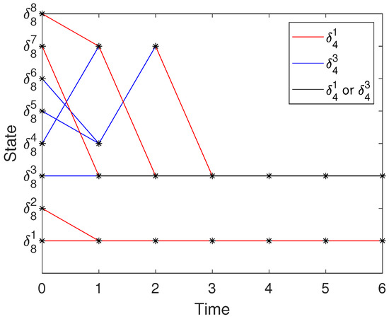
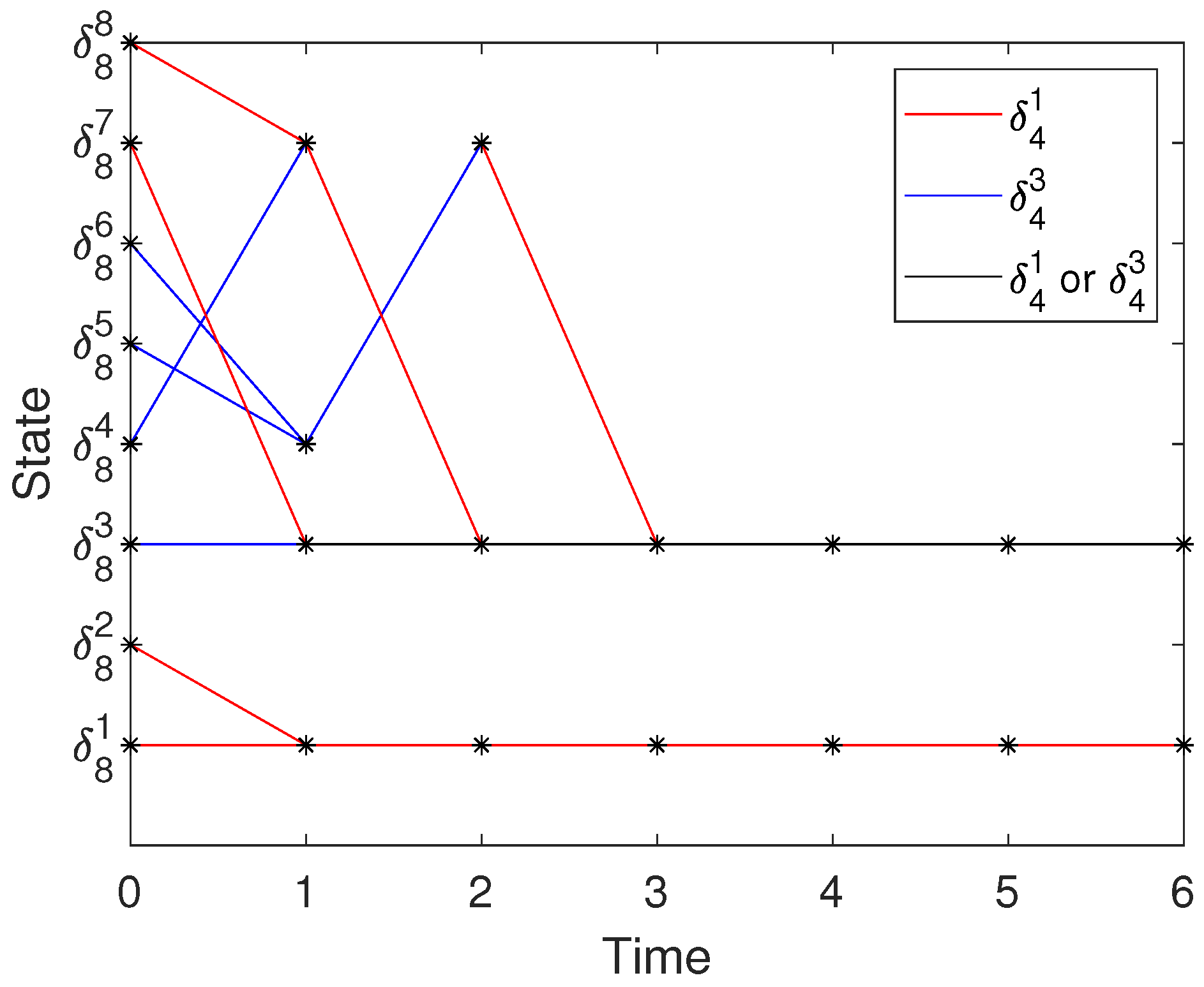
Under the above STC scheme (33), PBCN (28) can be stabilized to target set . The state trajectory of system (28) under STC (33) can be shown by Figure 1. As shown in Figure 1, under our proposed control strategy, the state trajectories starting from any initial state converge to the control invariant set . Furthermore, it can be seen from Figure 1 that, starting from any initial state, we can obtain the control inputs selected during the evolution and the maximum implementable steps of each control input. For example, for state , control is selected and implemented for 2 steps, and then control is chosen continuously. Then state can evolve to the control invariant set and remain in permanently.
Figure 1.
The trajectory graph of PBCN (28) under STC.
According to [6,22], we can design the state feedback control
such that PBCN (28) is stabilized to set with probability one. The control update instants of each state for PBCN (28) under the state feedback control (34) and STC (33) are listed in Table 1. Taking state as an example, the control needs to be updated three times to reach set under state feedback control (34). By contrast, for the STC we designed, only two control updates are required for state to arrive at set . It should be pointed out that for PBCN (28), a sampled-data controller with a fixed sampling period cannot be designed to stabilize the system to set with probability one. Example 1 demonstrates that STC can reduce the frequency of control updates and is more suitable for practical applications than sampled control.
Table 1.
The control update instants.
5. Conclusions
This paper has constructed a self-triggered control framework to determine set stabilization with probability one of PBCNs. We have put forward a constructive algorithm that generates LFs via a sequence of truth matrices and have further derived an LF-based necessary and sufficient condition for verifying whether a PBCN can be stabilized to a target set with probability one. Compared with the existing LF construction methods in the relevant literature, the proposed algorithm has exhibited superior implementability in practical computation. Furthermore, we have developed a complete procedure to design STCs. Since n-player random evolutionary games constitute a class of PBCNs, the results obtained in this paper can be applied to the self-triggered control design for convergence problems of n-player random evolutionary games.
The scalability is a key limitation of the proposed method. Since the number of states grows exponentially with the number of nodes in PBCNs, the computational burden increases rapidly for networks with more nodes. For future work, we will explore effective strategies to extend the current framework to larger-scale PBCNs. Potential directions include state reduction techniques and network aggregation schemes to reduce computational complexity.
Author Contributions
X.L.: Methodology, Formal analysis, Investigation, Resources, Writing—original draft; L.D.: Conceptualization, Software, Validation; H.K.: Writing—review and editing, Supervision. All authors have read and agreed to the published version of the manuscript.
Funding
This work is supported by the National Natural Science Foundation of China under Grant 62103176, and the Natural Science Foundation of Shandong Province under Grant ZR2024QF178.
Data Availability Statement
The code used for numerical simulation is available from the corresponding author upon reasonable request. No new dataset was generated.
Conflicts of Interest
The authors declare no conflict of interest.
References
- Shmulevich, I.; Dougherty, E.R.; Kim, S.; Zhang, W. Probabilistic Boolean networks: A rule-based uncertainty model for gene regulatory networks. Bioinformatics 2002, 18, 261–274. [Google Scholar] [CrossRef] [Scilit] [PubMed]
- Trairatphisan, P.; Mizera, A.; Pang, J.; Tantar, A.A.; Schneider, J.; Sauter, T. Recent development and biomedical applications of probabilistic Boolean networks. Cell Commun. Signal. 2013, 11, 46. [Google Scholar] [CrossRef] [Scilit] [PubMed]
- Chakraborty, A.; Hore, A.; Ganguly, C.; Chakrabarti, S. Probabilistic boolean operations in spiking neurons for neuromorphic systems. IEEE Trans. Emerg. Top. Comput. Intell. 2024, 8, 4250–4260. [Google Scholar] [CrossRef] [Scilit]
- Gu, J.-W.; Ching, W.-K.; Siu, T.-K.; Zheng, H. On modeling credit defaults: A probabilistic Boolean network approach. Risk Decis. Anal. 2013, 4, 119–129. [Google Scholar] [CrossRef] [Scilit]
- Elowitz, M.B.; Levine, A.J.; Siggia, E.D.; Swain, P.S. Stochastic gene expression in a single cell. Science 2002, 297, 1183–1186. [Google Scholar] [CrossRef] [Scilit] [PubMed]
- Wang, J.; Liu, W.; Fu, S.; Xia, J. On robust set stability and set stabilization of probabilistic Boolean control networks. Appl. Math. Comput. 2022, 422, 126992. [Google Scholar] [CrossRef] [Scilit]
- Zhao, Y.; Cheng, D. On controllability and stabilizability of probabilistic Boolean control networks. Sci. China Inf. Sci. 2014, 57, 1–14. [Google Scholar] [CrossRef] [Scilit]
- Zhou, R.; Guo, Y.; Gui, W. Set reachability and observability of probabilistic Boolean networks. Automatica 2019, 106, 230–241. [Google Scholar] [CrossRef] [Scilit]
- Li, Y.; Cheng, Y.; Li, H.; Yang, Z.; Huang, T. Disturbance Decoupling of Probabilistic Boolean Networks. IEEE Trans. Syst. Man. Cybern. Syst. 2025, 55, 8587–8598. [Google Scholar] [CrossRef] [Scilit]
- Li, H.; Wang, Y.; Guo, P. State feedback based output tracking control of probabilistic Boolean networks. Inf. Sci. 2016, 349, 1–11. [Google Scholar] [CrossRef] [Scilit]
- Deng, L.; Fu, S.; Li, X.; Wang, J. A matrix approach to the analysis and computation of robust cycles for Boolean control networks with disturbances. J. Appl. Math. Comput. 2024, 70, 4827–4850. [Google Scholar] [CrossRef] [Scilit]
- Fu, S.; Cheng, D.; Feng, J.-E.; Zhao, J. Matrix expression of finite Boolean-type algebras. Appl. Math. Comput. 2021, 395, 125880. [Google Scholar] [CrossRef] [Scilit]
- Sun, Y.; Fu, S.; Xia, L.; Xu, J. Minimal observability of switching Boolean networks. Math. Methods Appl. Sci. 2025, 48, 3291–3303. [Google Scholar] [CrossRef] [Scilit]
- Fu, S.; Wang, J.; Wang, Z.; Del Vecchio, C.; Zhao, J. Equilibrium existence and convergence of congestion games with stochastic disturbances. Sci. China Inf. Sci. 2026, 69, 140209. [Google Scholar] [CrossRef] [Scilit]
- Fu, S.; Li, L.; Feng, J.-E. Strategy optimization of controlled evolutionary games on a two-layer coupled network using lebesgue sampling. Nonlinear Anal. Hybrid Syst. 2025, 56, 101570. [Google Scholar] [CrossRef] [Scilit]
- Wang, D.; Fu, S.; Wang, J.; Li, Y.; Wang, Z. The stability degree analysis of profiles for networked evolutionary games with switching topology. Nonlinear Anal. Hybrid Syst. 2023, 50, 101396. [Google Scholar] [CrossRef] [Scilit]
- Zhou, Z.; Meng, Z.; Zhang, Y.; Song, Y.; Zhang, F. Real algorithms for special least squares solutions of the complex split quaternion matrix equations AX = B and AXC = B. Numer. Algorithms 2026, 102, 505–530. [Google Scholar] [CrossRef] [Scilit]
- Ding, W.; Li, Y.; Liu, Z.; Tao, R.; Zhang, M. Algebraic method for LU decomposition in commutative quaternion based on semi-tensor product of matrices and application to strict image authentication. Math. Methods Appl. Sci. 2024, 47, 6036–6050. [Google Scholar] [CrossRef] [Scilit]
- Yu, M.; Xia, J.; Feng, J.-E.; Fu, S.; Shen, H. Leader–follower output consensus of multiagent systems over finite fields. Neurocomputing 2023, 550, 126495. [Google Scholar] [CrossRef] [Scilit]
- Sun, Q.; Hou, W.; Li, H.; Wang, J. Finite-time set stabilization of impulsive probabilistic Boolean control networks via time-variant feedback control. Int. J. Control Autom. Syst. 2022, 20, 3592–3605. [Google Scholar] [CrossRef] [Scilit]
- Liu, W.; Feng, J.-E.; De Leone, R.; Fu, S.; Xia, J. Iterative algorithms for set stabilization of probabilistic Boolean control networks and applications in state-based games. IEEE Trans. Syst. Man Cybern. Syst. 2025, 55, 7048–7059. [Google Scholar] [CrossRef] [Scilit]
- Tian, H.; Hou, Y. State feedback design for set stabilization of probabilistic Boolean control networks. J. Frankl. Inst. 2019, 356, 4358–4377. [Google Scholar] [CrossRef] [Scilit]
- Liu, Y.; Wang, L.; Lu, J.; Cao, J. Sampled-data stabilization of probabilistic Boolean control networks. Syst. Control Lett. 2019, 124, 106–111. [Google Scholar] [CrossRef] [Scilit]
- Meng, M.; Xiao, G.; Cheng, D. Self-triggered scheduling for Boolean control networks. IEEE Trans. Cybern. 2021, 52, 8911–8921. [Google Scholar] [CrossRef] [Scilit] [PubMed]
- Li, X.; Fu, S.; Wang, J.; Zhang, F. Self-triggered control for the convergence of n-person random evolutionary games. Commun. Nonlinear Sci. Numer. Simul. 2025, 152, 109293. [Google Scholar] [CrossRef] [Scilit]
- Li, X.; Cao, X.; Fu, S.; Feng, J.; Zhao, X.; Wu, Q. Set stabilization of Boolean control networks with disturbance inputs via self-triggered control. Trans. Inst. Meas. Control 2026. [Google Scholar] [CrossRef] [Scilit]
- Acernese, A.; Yerudkar, A.; Glielmo, L.; Del Vecchio, C. Model-free self-triggered control co-design for probabilistic Boolean control networks. IEEE Control Syst. Lett. 2020, 5, 1639–1644. [Google Scholar] [CrossRef] [Scilit]
- Zhang, Q.; Yu, Y.; Feng, J.-E. Self-triggered control for approximate synchronization of singular logical networks. Nonlinear Anal. Hybrid Syst. 2024, 54, 101531. [Google Scholar] [CrossRef] [Scilit]
- Chen, B.; Cao, J.; Lu, G.; Rutkowski, L. Lyapunov functions for the set stability and the synchronization of Boolean control networks. IEEE Trans. Circuits Syst. II Express Briefs 2019, 67, 2537–2541. [Google Scholar] [CrossRef] [Scilit]
- Cheng, D.; Qi, H.; Li, Z. Analysis and Control of Boolean Networks: A Semi-Tensor Product Approach; Springer: London, UK, 2011. [Google Scholar]
- Li, R.; Yang, M.; Chu, T. State feedback stabilization for probabilistic Boolean networks. Automatica 2014, 50, 1272–1278. [Google Scholar] [CrossRef] [Scilit]
- Lin, L.; Cao, J.; Rutkowski, L. Robust event-triggered control invariance of probabilistic Boolean control networks. IEEE Trans. Neural Netw. Learn. Syst. 2019, 31, 1060–1065. [Google Scholar] [CrossRef] [Scilit] [PubMed]
- Li, W. Robust set stability of large-scale Boolean networks with disturbance via network aggregation. Int. J. Control 2025, 98, 474–480. [Google Scholar] [CrossRef] [Scilit]
- Li, H.; Wang, Y. Output feedback stabilization control design for Boolean control networks. Automatica 2013, 49, 3641–3645. [Google Scholar] [CrossRef] [Scilit]

Disclaimer/Publisher’s Note: The statements, opinions and data contained in all publications are solely those of the individual author(s) and contributor(s) and not of MDPI and/or the editor(s). MDPI and/or the editor(s) disclaim responsibility for any injury to people or property resulting from any ideas, methods, instructions or products referred to in the content. |
© 2026 by the authors. Licensee MDPI, Basel, Switzerland. This article is an open access article distributed under the terms and conditions of the Creative Commons Attribution (CC BY) license.