Parametric Inference of the Power Weibull Survival Model Using a Generalized Censoring Plan: Three Applications to Symmetry and Asymmetry Scenarios

Abstract

Generalized censoring, combined with a power-based distribution, improves inferential efficiency by capturing more detailed failure-time information in complex testing scenarios. Conventional censoring schemes may discard substantial failure-time information, leading to inefficiencies in parameter estimation and reliability prediction. To address this limitation, we develop a comprehensive inferential framework for the alpha-power Weibull (APW) distribution under a generalized progressive hybrid Type-II censoring scheme, a flexible design that unifies classical, hybrid, and progressive censoring while guaranteeing test completion within preassigned limits. Both maximum likelihood and Bayesian estimation procedures are derived for the model parameters, reliability function, and hazard rate. Associated uncertainty quantification is provided through asymptotic confidence intervals (normal and log-normal approximations) and Bayesian credible intervals obtained via Markov chain Monte Carlo (MCMC) methods with independent gamma priors. In addition, we propose optimal censoring designs based on trace, determinant, and quantile-variance criteria to maximize inferential efficiency at the design stage. Extensive Monte Carlo simulations, assessed using four precision measures, demonstrate that the Bayesian MCMC estimators consistently outperform their frequentist counterparts in terms of bias, mean squared error, robustness, and interval coverage across a wide range of censoring levels and prior settings. Finally, the proposed methodology is validated using real-life datasets from engineering (electronic devices), clinical (organ transplant), and physical (rare metals) studies, demonstrating the APW model’s superior goodness-of-fit, reliability prediction, and inferential stability. Overall, this study demonstrates that combining generalized censoring with the APW distribution substantially enhances inferential efficiency and predictive performance, offering a robust and versatile tool for complex life-testing experiments across multiple scientific domains.

1. Introduction

In many practical studies, complete failure-time information for experimental units is often unavailable. To minimize cost and shorten experimental duration, censoring strategies are typically employed. The two standard censoring methods, Type-I (time-based) and Type-II (failure-based), have been extensively analyzed by Bain and Engelhardt [1]. Later, Epstein [2] and Childs et al. [3] proposed their hybrid extensions, known respectively as the hybrid Type-I (TI-H) and hybrid Type-II (TII-H) censoring schemes. Although widely used, these classical schemes do not allow the removal of surviving units at arbitrary times before the end of the test, thereby limiting flexibility and reducing efficiency in practical applications. To enhance design adaptability, making use of Type-I progressive censoring (TII-PC), Balakrishnan and Cramer [4] explored the progressive versions of these censoring models and their hybrid forms; namely, the Type-I progressive hybrid censoring (TI-PHC) and Type-II progressive hybrid censoring (TII-PHC) schemes. Despite their practical importance, TI-PHC and TII-PHC schemes often exhibit very long testing times, hindering effective inference. To overcome this limitation, Ng et al. [5] developed the adaptive TII-PHC (ATII-PHC) scheme, which achieves shorter test times and improved efficiency.

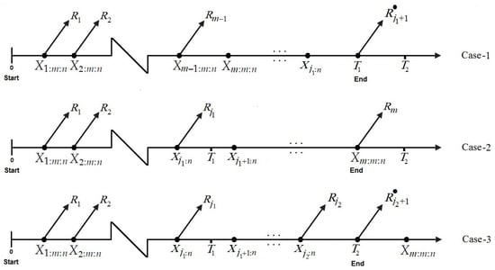
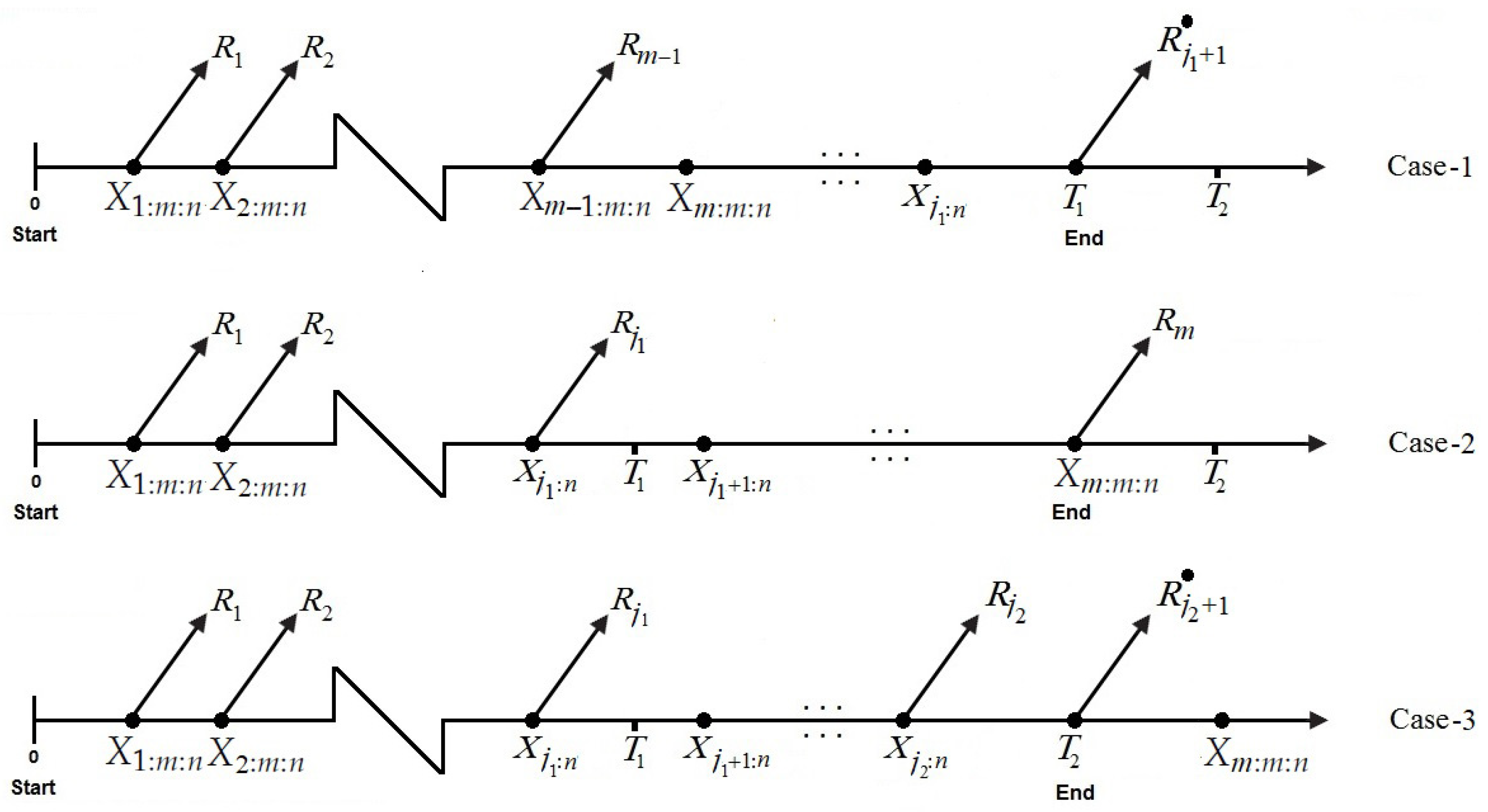
However, both TII-PHC and ATII-PHC plans still require observing a fixed number of m failures, potentially extending the overall test time. To ensure that experiments end within a predetermined time frame, Lee et al. [6] proposed the generalized-T2PH (GTII-PHC) scheme, which guarantees test termination at a fixed time, thereby reducing both cost and duration. The GTII-PHC design is described as follows: consider n units placed on a life test at time zero, with $m(<n)$ observed failures and a progressive censoring plan $\mathbf{R}=(R_1,\dots ,R_m)$. Two predetermined times $T_1$ and $T_2$ are selected such that $0<T_1<T_2<\infty$, and let $(j_1,j_2)$ represent the numbers of observed failures before $T_1$ and $T_2$, respectively. Following each observed failure (e.g., $X_{j:m:n}$), a fixed number $R_j$ of surviving units are randomly withdrawn from the test. The experiment concludes at ${\mathcal{T}}^{•}=max\left\{T_1,min\left\{X_{m:m:n},T_2\right\}\right\}$ where $T_2$ denotes the maximum time permitted for the continuation of the experiment. If $X_{m:m:n}<T_1$, the experiment proceeds with additional failure observations and no further withdrawals until time $T_1$ (Case 1). If $T_1<X_{m:m:n}<T_2$, the test is terminated at the m-th failure time, $X_{m:m:n}$ (Case 2). Otherwise, if $X_{m:m:n}>T_2$, the experiment concludes at the predetermined time $T_2$ (Case 3). It is noteworthy that the GTII-PHC scheme modifies the conventional TII-PHC design by guaranteeing termination of the test at the fixed time $T_2$, representing the maximum duration the experimenter is willing to allow. A schematic representation of GTII-PHC is depicted in Figure 1.

Figure 1. Schematic representation of the GTII-PHC plan.

Consequently, the experimenter encounters one of the following three data configurations:

$$\{\mathbf{X},\mathbf{R}\}=\left\{\begin{array}{ccc}\{(X_{1:m:n},R_1),\dots ,(X_{m-1:m:n},R_{m-1}),(X_{m:m:n},0),\dots ,(X_{j_1:n},0)\};\hfill & & \mathrm{Case}\text{-}1,\\ \{(X_{1:m:n},R_1),\dots ,(X_{j1:n},R_{j_1}),\dots ,(X_{m-1:m:n},R_{m-1}),(X_{m:m:n},R_m)\};\hfill & & \mathrm{Case}\text{-}2,\\ \{(X_{1:m:n},R_1),\dots ,(X_{j_1:n},R_{j_1}),\dots ,(X_{j_2-1:n},R_{j_2-1}),(X_{j_2:n},R_{j_2})\};\hfill & & \mathrm{Case}\text{-}3.\end{array}\right.$$

Assume that $\{\mathbf{X},\mathbf{R}\}$ represents the observed lives and the corresponding removed units from a sample having cumulative distribution function (CDF), $F(·)$, and probability density function (PDF), $f(·)$. The likelihood function (LF) of the GTII-PHC is:

$${\mathcal{L}}_{\tau }(\mathit{\theta }\mid \mathbf{x})=M_{\tau }\mathcal{R}\tau (T_k;\mathit{\theta }){\prod }_{i=1}^{Q_{\tau }}f(x_{i:m:n};\mathit{\theta }){\left[1-F(x_{i:m:n};\mathit{\theta })\right]}^{R_i},\tau =1,2,3,k=1,2,$$

(1)

where, in Table 1, the notations in Equation (1) are defined. Furthermore, from (1), we have:

Table 1. The notations of the GTII-PHC likelihood function.

$\mathit{\tau }$	${\mathit{M}}_{\mathit{\tau }}$	${\mathit{Q}}_{\mathit{\tau }}$	${\mathcal{R}}_{\mathit{\tau }}({\mathit{T}}_{\mathit{k}};\mathit{\theta })$	${\mathit{R}}_{{\mathit{j}}_{\mathit{k}}+1}^{•}$
1	${\mathrm{\Pi }}_{o=1}^{j_1}{\sum }_{i=o}^m\left(R_i+1\right)$	$j_1$	${\left[1-F\left(T_1\right)\right]}^{R_{j_1+1}^{•}}$	$n-j_1-{\sum }_{i=1}^{m-1}{R}_i$
2	${\mathrm{\Pi }}_{o=1}^m{\sum }_{i=o}^m\left(R_i+1\right)$	m	1	0
3	${\mathrm{\Pi }}_{o=1}^{j_2}{\sum }_{i=o}^m\left(R_i+1\right)$	$j_2$	${\left[1-F\left(T_2\right)\right]}^{R_{j_2+1}^{•}}$	$n-j_2-{\sum }_{i=1}^{j_2}{R}_i$

• TI-PHC, when $T_1\to 0$; and TII-PHC, when $T_2\to \infty$;
• Hybrid Type-I censoring, when $T_1\to 0$, $R_i=0$ for $i=1,2,\dots ,m-1$;
• Hybrid Type-II censoring, when $T_2\to \infty$, $R_i=0$ for $i=1,2,\dots ,m-1$;
• Type-I censoring, when $T_1=0$, $m=1$, $R_i=0$ for $i=1,2,\dots ,m-1$;
• Type-II censoring, when $T_1=0$, $T_2\to \infty$, $R_i=0$ for $i=1,2,\dots ,m-1$.

Although several censoring mechanisms have been proposed in the literature, the GTII-PHC plan adopted in this study offers two practical advantages in survival experimentation. First, it provides high experimental-design flexibility by simultaneously fixing the maximum test time and controlling the number and timing of withdrawals, which allows researchers to balance cost, risk, and expected test duration more transparently than adaptive censoring, where rules change dynamically and may complicate test planning. Second, the GTII-PHC structure ensures efficient information utilization by retaining failure information across the entire testing horizon, particularly in the tail region, whereas adaptive schemes often terminate early or ignore late-time information when operating thresholds are reached. These properties make GTII-PHC a robust and tractable design for likelihood-based inference.

Several studies based on the GTII-PHC have been conducted to explore different lifetime models and estimation techniques. For instance, Ateya and Mohammed [7] and Nagy et al. [8] (for Burr–XII); Cho and Lee [9] (for exponential competing risks); Wang et al. [10], Alqasem et al. [11], and Mohammed et al. [12] considered the estimation issue of the Kumaraswamy, Garima, and log-logistic parameters, respectively.

In the statistical distribution literature, significant progress has been made in extending classical probability distributions and applying them efficiently in diverse fields such as engineering, medicine, finance, and others. Among these flexible models, the alpha–power Weibull (APW) distribution, suggested by Nassar et al. [13] through the alpha power transformation proposed by Mahdavi and Kundu [14], has attracted considerable attention. This distribution serves as a generalization of the traditional Weibull model and provides enhanced flexibility in modeling various shapes of the probability density and hazard rate functions. If X is a lifetime random variable following the APW model, its PDF and CDF, where $\mathit{\theta }={(\alpha ,\delta ,\vartheta )}^{\top }$, are respectively given by

$$f(x;\mathit{\theta })={\displaystyle \frac{\vartheta \delta \log \left(\alpha \right)x^{\delta -1}\exp (-\vartheta x^{\delta }){\alpha }^{1-\exp (-\vartheta x^{\delta })}}{\alpha -1}},$$

(2)

and

$$F(x;\mathit{\theta })={\displaystyle \frac{{\alpha }^{1-\exp (-\vartheta x^{\delta })}-1}{\alpha -1}},$$

(3)

where $x>0,\alpha ,\delta ,\vartheta >0,\mathrm{a}\mathrm{n}\mathrm{d}\alpha \ne 1$.

Assessing the reliability function (RF) and hazard rate function (HRF) provides critical insights into the survival behavior and failure dynamics of a system over time. While the reliability function quantifies the probability of a component operating without failure up to a specified time, the hazard rate function characterizes the instantaneous risk of failure, enabling a deeper understanding of model adequacy and maintenance planning. The RF $R\left(t\right)$ and HRF $h\left(t\right)$ (for a mission time $t>0$) of the APW distribution are respectively defined as

$$R(t;\mathit{\theta })={\displaystyle \frac{\alpha }{\alpha -1}}\left(1-{\alpha }^{-\exp (-\vartheta t^{\delta })}\right),$$

(4)

and

$$h(t;\mathit{\theta })={\displaystyle \frac{\vartheta \delta \log \left(\alpha \right)t^{\delta -1}\exp (-\vartheta t^{\delta })}{{\alpha }^{\exp (-\vartheta t^{\delta })}-1}}.$$

(5)

Reliability experiments and life-testing studies often encounter situations where the lifetimes of test units are incompletely observed due to time or cost limitations. To address this, the GTII-PHC provides a more inclusive and adaptable structure that incorporates the strengths of both Type-II and hybrid designs while allowing progressive removals. Meanwhile, the APW distribution, as a generalization of the alpha-power exponential and classical Weibull model, offers substantial flexibility in modeling diverse lifetime behaviors through its additional shape parameter.

By integrating the GTII–PHC with the APW formulation, the present study provides three notable methodological improvements. First, the proposed APW model integrates the proportional-hazards structure with an enhanced shape parameterization, offering significantly richer hazard shapes than those developed by the traditional Weibull hazard rate patterns. Second, by incorporating the three-parameter model within a generalized censoring plan, we achieve markedly improved estimation efficiency, since the likelihood construction utilizes both early and late censoring information without the need for adaptive conditioning strategies. Third, the proposed inferential methodologies extend the application scope by enabling coherent treatment of symmetric and asymmetric survival scenarios, demonstrated through three diverse real-data applications. Together, these developments provide a unified and computationally tractable modeling framework that exceeds the flexibility, estimation stability, and empirical adaptability reported in the existing literature.

However, to date, no comprehensive statistical treatment has examined APW data under GTII-PHC settings. This feature motivates the present study, which integrates the modeling power of the APW distribution with the practicality and information efficiency of the GTII-PHC scheme, providing a robust inferential framework for reliability and engineering data. The key contributions of this work can be summarized as follows:

• Develop a new framework for APW allocation under the GTII-PHC mechanism, which includes several existing censoring and hybrid schemes as special cases.
• The maximum likelihood estimators (MLEs) for the model parameters, as well as the related reliability and hazard rate functions, are derived, together with their asymptotic confidence intervals (ACIs).
• Formulation of Bayesian estimation procedures using independent gamma priors, implemented through a Metropolis–Hastings (M–H)-based Markov Chain Monte Carlo (MCMC) algorithm to obtain posterior means, Bayesian credible intervals (BCIs), and highest posterior density (HPD) intervals.
• Establishment of reliability insights indicating that the Bayesian MCMC estimation approach under informative gamma priors yields more accurate and stable parameter and reliability estimates compared to classical methods.
• Execution of extensive simulations to evaluate and compare the performance of the proposed MLE and Bayesian estimators under various censoring schemes, sample sizes, and prior configurations.
• Investigation of optimum censoring plans by employing multiple criteria (trace, determinant, and quantile-variance-based), to identify information-efficient experimental designs.
• Application of the proposed methodology to real-life datasets from three sciences, demonstrating the practical relevance and superior fitting performance of the APW model under GTII-PHC data.

The paper is structured as follows: Section 2 and Section 3 discuss likelihood and Bayesian inferences, respectively; Section 4 covers various interval estimation methods; Section 5 presents results from Monte Carlo simulations; Section 6 analyzes two real data applications to illustrate method usefulness; Section 7 reports several optimum criteria; and Section 8 concludes with remarks and recommendations.

2. Likelihood Estimation

Let $\mathbf{x}=(X_{1:m:n},R_1),\dots ,(X_{j_1:n},R_{j_1}),\dots ,(X_{j_2:n},R_{j_2})$ denote a GTII-PHC dataset of size $j_2$ drawn from $\mathrm{APW}\left(\mathit{\theta }\right)$. Accordingly, by substituting (2) and (3) into (1), using $x_i$ in place of $x_{i:m:n}$, the GTII-PHC’s LF strategy can be expressed as

$${\mathcal{L}}_{\tau }\left(\mathit{\theta }|\mathbf{x}\right)\propto {\mathrm{{\rm Y}}}_{\tau }\left(T_k;\mathit{\theta }\right){\left({\displaystyle \frac{\alpha }{\alpha -1}}\right)}^n{\left(\vartheta \delta \log \left(\alpha \right)\right)}^{Q_{\tau }}{e}^{-\vartheta {\sum }_{i=1}^{Q_{\tau }}{x}_i^{\delta }}\prod _{i=1}^{Q_{\tau }}{x}_i^{\delta }{\alpha }^{1-\exp \left(-\vartheta x_i^{\delta }\right)}{\left(\omega \left(x_i;\mathit{\theta }\right)\right)}^{R_i},$$

(6)

where $\omega \left(x_i;\mathit{\theta }\right)=1-{\alpha }^{-\exp \left(-\vartheta x_i^{\delta }\right)}$, ${\mathrm{{\rm Y}}}_{\tau }\left(T_k;\mathit{\theta }\right)={\left[{\displaystyle \frac{\alpha \omega \left(T_k;\mathit{\theta }\right)}{\alpha -1}}\right]}^{R_{j_k+1}^{•}},k=1,2,$ and ${\mathrm{{\rm Y}}}_2\left(T_k;\mathit{\theta }\right)=1$.

The equivalent log-LF (say, ${\mathcal{L}}_{\tau }^{★}\propto \log {\mathcal{L}}_{\tau }$) of (6) becomes

$$\begin{array}{cc}\hfill {\mathcal{L}}_{\tau }^{★}\left(\mathit{\theta }|\mathbf{x}\right)& \propto {\psi }_{\tau }\left(T_k;\mathit{\theta }\right)+n\log \left({\displaystyle \frac{\alpha }{\alpha -1}}\right)+Q_{\tau }\log \left(\vartheta \delta \log \left(\alpha \right)\right)\hfill \\ \hfill & -\vartheta \sum _{i=1}^{Q_{\tau }}{x}_i^{\delta }+\delta \sum _{i=1}^{Q_{\tau }}\log \left(x_i\right)-\log \left(\alpha \right)\sum _{i=1}^{Q_{\tau }}{e}^{-\vartheta x_i^{\delta }}+\sum _{i=1}^{Q_{\tau }}{R}_i\log \left(\omega \left(x_i;\mathit{\theta }\right)\right),\hfill \end{array}$$

(7)

where ${\psi }_{\tau }\left(T_k;\mathit{\theta }\right)=\log \left({\mathrm{{\rm Y}}}_{\tau }\left(T_k;\mathit{\theta }\right)\right)$.

By partially differentiating (7) with respect to $\alpha$, $\delta$, and $\vartheta$, the following three equations are obtained. Setting these derivatives equal to zero and solving algebraically yields the MLEs $\widehat{\alpha }$, $\widehat{\delta }$, and $\widehat{\vartheta }$ of $\alpha$, $\delta$, and $\vartheta$, respectively, as follows:

$$\begin{array}{c}\hfill {\displaystyle \frac{\partial {\mathcal{L}}_{\tau }^{★}}{\partial \alpha }}={\psi }_{\tau }^{\alpha }\left(T_k;\mathit{\theta }\right)+n\left({\displaystyle \frac{1}{\alpha }}-{\displaystyle \frac{1}{\alpha -1}}\right)+{\displaystyle \frac{Q_{\tau }}{\alpha \log \left(\alpha \right)}}-{\displaystyle \frac{1}{\alpha }}\sum _{i=1}^{Q_{\tau }}{e}^{-\vartheta x_i^{\delta }}+\sum _{i=1}^{Q_{\tau }}{R}_i\left({\displaystyle \frac{{\omega }_{\alpha }^{\circ }\left(x_i;\mathit{\theta }\right)}{\omega \left(x_i;\mathit{\theta }\right)}}\right),\end{array}$$

(8)

$$\begin{array}{c}\hfill {\displaystyle \frac{\partial {\mathcal{L}}_{\tau }^{★}}{\partial \delta }}={\psi }_{\tau }^{\delta }\left(T_k;\mathit{\theta }\right)+{\displaystyle \frac{Q_{\tau }}{\delta }}-\vartheta \sum _{i=1}^{Q_{\tau }}{x}_i^{\delta }\log \left(x_i\right)\left[1+\log \left(\alpha \right)e^{-\vartheta x_i^{\delta }}\right]+\sum _{i=1}^{Q_{\tau }}{R}_i\left({\displaystyle \frac{{\omega }_{\delta }^{\circ }\left(x_i;\mathit{\theta }\right)}{\omega \left(x_i;\mathit{\theta }\right)}}\right),\end{array}$$

(9)

and

$$\begin{array}{c}\hfill {\displaystyle \frac{\partial {\mathcal{L}}_{\tau }^{★}}{\partial \vartheta }}={\psi }_{\tau }^{\vartheta }\left(T_k;\mathit{\theta }\right)+{\displaystyle \frac{Q_{\tau }}{\vartheta }}-\sum _{i=1}^{Q_{\tau }}{x}_i^{\delta }+\log \left(\alpha \right)\sum _{i=1}^{Q_{\tau }}{x}_i^{\delta }{e}^{-\vartheta x_i^{\delta }}+\sum _{i=1}^{Q_{\tau }}{R}_i\left({\displaystyle \frac{{\omega }_{\delta }^{\circ }\left(x_i;\mathit{\theta }\right)}{\omega \left(x_i;\mathit{\theta }\right)}}\right),\end{array}$$

(10)

where for $k=1,3$ and $\tau =1,2,3$, we have

$$\begin{array}{cc}\hfill & {\omega }_{\alpha }^{\circ }\left(x_i;\mathit{\theta }\right)=e^{-\vartheta x_i^{\delta }}{\alpha }^{-\exp \left(-\vartheta x_i^{\delta }\right)-1},{\omega }_{\delta }^{\circ }\left(x_i;\mathit{\theta }\right)=-\vartheta x_i^{\delta }\log \left(x_i\right)\log \left(\alpha \right)e^{-\vartheta x_i^{\delta }}{\alpha }^{-\exp \left(-\vartheta x_i^{\delta }\right)-1},\hfill \\ \hfill & {\omega }_{\vartheta }^{\circ }\left(x_i;\mathit{\theta }\right)=-x_i^{\delta }\log \left(\alpha \right)e^{-\vartheta x_i^{\delta }}{\alpha }^{-\exp \left(-\vartheta x_i^{\delta }\right)-1},\hfill \\ \hfill & {\psi }_{\tau }^{\alpha }\left(T_k;\mathit{\theta }\right)={\displaystyle \frac{1}{\alpha -1}}\left[e^{-\vartheta T_k^{\delta }}{\alpha }^{-\exp \left(-\vartheta T_k^{\delta }\right)}-{\displaystyle \frac{1}{\alpha -1}}\left(1-{\alpha }^{-\exp \left(-\vartheta T_k^{\delta }\right)}\right)\right]R_{j_k+1}^{•}{\mathrm{{\rm Y}}}_{\tau }^{-1}\left(T_k;\mathit{\theta }\right),\hfill \\ \hfill & {\psi }_{\tau }^{\delta }\left(T_k;\mathit{\theta }\right)=-{\displaystyle \frac{\alpha \vartheta }{\alpha -1}}{T}_k^{\delta }\log \left(T_k\right)\log \left(\alpha \right)e^{-\vartheta T_k^{\delta }}{\alpha }^{-\exp \left(-\vartheta T_k^{\delta }\right)}{R}_{j_k+1}^{•}{\mathrm{{\rm Y}}}_{\tau }^{-1}\left(T_k;\mathit{\theta }\right),\hfill \\ \hfill & \mathrm{a}\mathrm{n}\mathrm{d}\hfill \\ \hfill & {\psi }_{\tau }^{\vartheta }\left(T_k;\mathit{\theta }\right)=-{\displaystyle \frac{\alpha }{\alpha -1}}{T}_k^{\delta }\log \left(\alpha \right)e^{-\vartheta T_k^{\delta }}{\alpha }^{-\exp \left(-\vartheta T_k^{\delta }\right)}{R}_{j_k+1}^{•}{\mathrm{{\rm Y}}}_{\tau }^{-1}\left(T_k;\mathit{\theta }\right).\hfill \end{array}$$

It is worth noting here that the proposed MLEs of $\alpha$, $\delta$, and $\vartheta$ inherit well-established large-sample properties under general censoring schemes. In particular, the MLEs for parametric lifetime models under progressive Type-II, hybrid, and generalized progressive hybrid censoring are known to be consistent and asymptotically normal, provided the number of observed failures increases with sample size and the censoring scheme satisfies standard information-regularity conditions. Consequently, the asymptotic variance of the proposed MLEs is obtained from the inverse of the observed Fisher information matrix, thereby justifying the use of normal-based confidence intervals and supporting the inferential validity of the proposed methodology; see, for instance, Balakrishnan and Cramer [4], and Peng and Chen [15].

After acquiring the MLEs $\widehat{\alpha }$, $\widehat{\delta }$, and $\widehat{\vartheta }$, the invariance property of the ML method is employed to derive the MLEs of the reliability $R\left(t\right)$ and hazard rate $h\left(t\right)$ functions, denoted by $\widehat{R}\left(t\right)$ and $\widehat{h}\left(t\right)$ for $t>0$, respectively as follows:

$$\widehat{R}\left(t\right)={\displaystyle \frac{\widehat{\alpha }}{\widehat{\alpha }-1}}\left(1-{\widehat{\alpha }}^{-\exp \left(-\widehat{\vartheta }{t}^{\widehat{\delta }}\right)}\right),\mathrm{a}\mathrm{n}\mathrm{d}\widehat{h}\left(t\right)={\displaystyle \frac{\widehat{\vartheta }\widehat{\delta }\log \left(\widehat{\alpha }\right)t^{\widehat{\delta }-1}\exp \left(-\widehat{\vartheta }{t}^{\widehat{\delta }}\right)}{{\widehat{\alpha }}^{\exp \left(-\widehat{\vartheta }{t}^{\widehat{\delta }}\right)}-1}}.$$

Since there are no closed-form expressions for $\widehat{\alpha }$, $\widehat{\delta }$, and $\widehat{\vartheta }$ in (8), (9), and (10), respectively, their estimators are determined by solving a multiple of nonlinear equations simultaneously. Consequently, these estimates must be obtained numerically, for instance, using the Newton-Raphson (NR) iterative method applied to each given GTII-PHC dataset. The NR iterative steps for calculating the MLEs $\widehat{\alpha }$, $\widehat{\delta }$, and $\widehat{\vartheta }$ are provided in Algorithm 1. The corresponding MLEs of $R\left(t\right)$ and $h\left(t\right)$ can then be derived by substituting $\widehat{\alpha }$, $\widehat{\delta }$, and $\widehat{\vartheta }$ in the place of $\alpha$, $\delta$, and $\vartheta$, respectively.

Algorithm 1 The NR Iterative Algorithm

1: Input: Set $\mathbf{x}$; log-likelihood ${\mathcal{L}}_{\tau }^{★}(·)$; tolerance $ϵ={10}^{-6}$   2: Output: Estimated parameter vector $\widehat{\mathit{\theta }}={(\widehat{\alpha },\widehat{\delta },\widehat{\vartheta })}^{\top }$   3: Step 1: Initialization   4: Obtain preliminary values from empirical summaries:     • Choose ${\alpha }^{\left(0\right)}$ by matching the first sample percentile to its theoretical analogue;     • Approximate ${\delta }^{\left(0\right)}$ from the slope of the log–log empirical hazard plot;     • Set ${\vartheta }^{\left(0\right)}$ as the reciprocal of the mean of uncensored observations.   5: Set initial vector ${\mathit{\theta }}^{\left(0\right)}={({\alpha }^{\left(0\right)},{\delta }^{\left(0\right)},{\vartheta }^{\left(0\right)})}^{\top }$.   6: Step 2: Iterative Update   7: for  $k=0,1,2,\dots$do   8:     Compute gradient ${\wp }^{\left(k\right)}={\displaystyle \frac{\partial }{\partial \mathit{\theta }}}{\mathcal{L}}_{\tau }^{★}\left({\mathit{\theta }}^{\left(k\right)}\right)$.   9:     Compute Hessian matrix ${\mathcal{H}}^{\left(k\right)}={\displaystyle \frac{{\partial }^2}{\partial {\mathit{\theta }}^2}}{\mathcal{L}}_{\tau }^{★}\left({\mathit{\theta }}^{\left(k\right)}\right)$. 10:     Solve the Newton direction: ${\zeta }^{\left(k\right)}=-{\left({\mathcal{H}}^{\left(k\right)}\right)}^{-1}{\wp }^{\left(k\right)}$. 11:     Propose update: ${\mathit{\theta }}_{\mathrm{prop}}^{(k+1)}={\mathit{\theta }}^{\left(k\right)}+{\zeta }^{\left(k\right)}$. 12:     Step 3: Numerical Stability 13:     if ${\mathcal{H}}^{\left(k\right)}$ is not negative definite or ${\mathcal{L}}_{\tau }^{★}\left({\mathit{\theta }}_{\mathrm{prop}}^{(k+1)}\right)<{\mathcal{L}}_{\tau }^{★}\left({\mathit{\theta }}^{\left(k\right)}\right)$ then 14:         Apply damping: ${\mathit{\theta }}^{(k+1)}={\mathit{\theta }}^{\left(k\right)}+\delta {\zeta }^{\left(k\right)}$ where $0<\delta <1$. 15:     else 16:         Accept update: ${\mathit{\theta }}^{(k+1)}={\mathit{\theta }}_{\mathrm{prop}}^{(k+1)}$. 17:     end if 18:     Step 4: Convergence Criterion 19:     if $\parallel {\mathit{\theta }}^{(k+1)}-{\mathit{\theta }}^{\left(k\right)}\parallel <ϵ$ or $|{\mathcal{L}}_{\tau }^{★}\left({\mathit{\theta }}^{(k+1)}\right)-{\mathcal{L}}_{\tau }^{★}\left({\mathit{\theta }}^{\left(k\right)}\right)| <ϵ$ then 20:         Stop and return $\widehat{\mathit{\theta }}={\mathit{\theta }}^{(k+1)}$. 21:     end if 22: end for

3. Bayes Inference

In this section, the Bayes estimators of $\alpha$, $\delta$, $\vartheta$, $R\left(t\right)$, and $h\left(t\right)$, along with their corresponding BCI and HPD interval estimates, are developed. To accomplish this, the parameters $\alpha$, $\delta$, and $\vartheta$ of the APW model are assumed to follow $G_i(a_i,b_i)$, for $i=1,2,3$. Several appealing properties justify the use of the gamma prior: (i) it can exhibit a wide range of shapes depending on the hyperparameter specifications, (ii) it provides sufficient flexibility for representing diverse prior beliefs, and (iii) it is analytically tractable and computationally stable, thus avoiding complex estimation challenges. Consequently, the joint gamma prior PDF of $\alpha$, $\delta$, and $\vartheta$ (say $\mathrm{\Phi }(·)$) is

$$\begin{array}{c}\hfill \mathrm{\Phi }\left(\mathit{\theta }\right)\propto {\alpha }^{a_1-1}{\delta }^{a_2-1}{\vartheta }^{a_3-1}{e}^{-(b_1\alpha +b_2\delta +b_3\vartheta )},\alpha ,\delta ,\vartheta >0,\end{array}$$

(11)

where $a_i>0$ and $b_i>0$ (for $i=1,2,3$) are known.

From (6) and (11), the joint posterior PDF of $\alpha$, $\delta$, and $\vartheta$ (say ${\mathcal{P}}_{\tau }(·)$) is

$$\begin{array}{cc}\hfill {\mathcal{P}}_{\tau }\left(\mathit{\theta }|\mathbf{x}\right)& \propto {\displaystyle \frac{{\alpha }^{n+Q_{\tau }+a_1-1}{\left(\log \left(\alpha \right)\right)}^{Q_{\tau }}}{{\left(\alpha -1\right)}^n}}{\delta }^{Q_{\tau }+a_2-1}{\vartheta }^{Q_{\tau }+a_3-1}{e}^{-(b_1\alpha +b_2\delta +b_3\vartheta )}{e}^{-\vartheta {\sum }_{i=1}^{Q_{\tau }}{x}_i^{\delta }}\hfill \\ \hfill & \times {\mathrm{{\rm Y}}}_{\tau }\left(T_k;\mathit{\theta }\right)\prod _{i=1}^{Q_{\tau }}{x}_i^{\delta }{\alpha }^{1-\exp \left(-\vartheta x_i^{\delta }\right)}{\left(\omega \left(x_i;\mathit{\theta }\right)\right)}^{R_i},\hfill \end{array}$$

(12)

where the associated normalized constant term (say, $\mathrm{\Xi }$) is given by

$$\begin{array}{c}\hfill \mathrm{\Xi }={\int }_0^{\infty }{\int }_0^{\infty }{\int }_0^{\infty }{\mathcal{P}}_{\tau }\left(\mathit{\theta }|\mathbf{x}\right)\mathrm{d}\alpha \mathrm{d}\delta \mathrm{d}\vartheta .\end{array}$$

Considering the squared–error loss, the Bayes estimator of $\alpha$ (as an example), denoted by $\tilde{\alpha }(·)$, is given by:

$$\tilde{\alpha }={\displaystyle \frac{1}{\mathrm{\Xi }}}{\int }_0^{\infty }{\int }_0^{\infty }{\int }_0^{\infty }\alpha \times {\mathcal{P}}_{\tau }\left(\mathit{\theta }|\mathbf{x}\right)\mathrm{d}\alpha \mathrm{d}\delta \mathrm{d}\vartheta .$$

(13)

It is evident from (12) that obtaining closed-form expressions for the three marginal PDFs of $\alpha$, $\delta$, and $\vartheta$ is analytically intractable. Therefore, to compute the corresponding Bayes estimates and construct their BCI and HPD intervals, we propose generating posterior samples from (12) using Bayesian MCMC techniques. Accordingly, the conditional posterior densities of $\alpha$, $\delta$, and $\vartheta$ are expressed, respectively, as

$${\mathcal{P}}_{\tau }^{\alpha }\left(\mathit{\theta }|\mathbf{x}\right)\propto {\displaystyle \frac{{\alpha }^{n+Q_{\tau }+a_1-1}{e}^{-b_1\alpha }{\left(\log \left(\alpha \right)\right)}^{Q_{\tau }}}{{\left(\alpha -1\right)}^n}}{\mathrm{{\rm Y}}}_{\tau }\left(T_k;\mathit{\theta }\right)\prod _{i=1}^{Q_{\tau }}{\alpha }^{1-\exp \left(-\vartheta x_i^{\delta }\right)}{\left(\omega \left(x_i;\mathit{\theta }\right)\right)}^{R_i},$$

(14)

$${\mathcal{P}}_{\tau }^{\delta }\left(\mathit{\theta }|\mathbf{x}\right)\propto {\delta }^{Q_{\tau }+a_2-1}{e}^{-\left(b_2\delta +\vartheta {\sum }_{i=1}^{Q_{\tau }}{x}_i^{\delta }\right)}{\mathrm{{\rm Y}}}_{\tau }\left(T_k;\mathit{\theta }\right)\prod _{i=1}^{Q_{\tau }}{x}_i^{\delta }{\alpha }^{1-\exp \left(-\vartheta x_i^{\delta }\right)}{\left(\omega \left(x_i;\mathit{\theta }\right)\right)}^{R_i},$$

(15)

and

$${\mathcal{P}}_{\tau }^{\vartheta }\left(\mathit{\theta }|\mathbf{x}\right)\propto {\vartheta }^{Q_{\tau }+a_3-1}{e}^{-\vartheta \left(b_3+{\sum }_{i=1}^{Q_{\tau }}{x}_i^{\delta }\right)}{\mathrm{{\rm Y}}}_{\tau }\left(T_k;\mathit{\theta }\right)\prod _{i=1}^{Q_{\tau }}{\alpha }^{1-\exp \left(-\vartheta x_i^{\delta }\right)}{\left(\omega \left(x_i;\mathit{\theta }\right)\right)}^{R_i}.$$

(16)

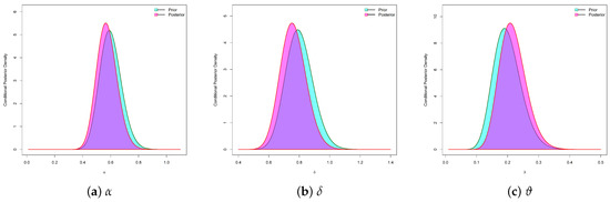
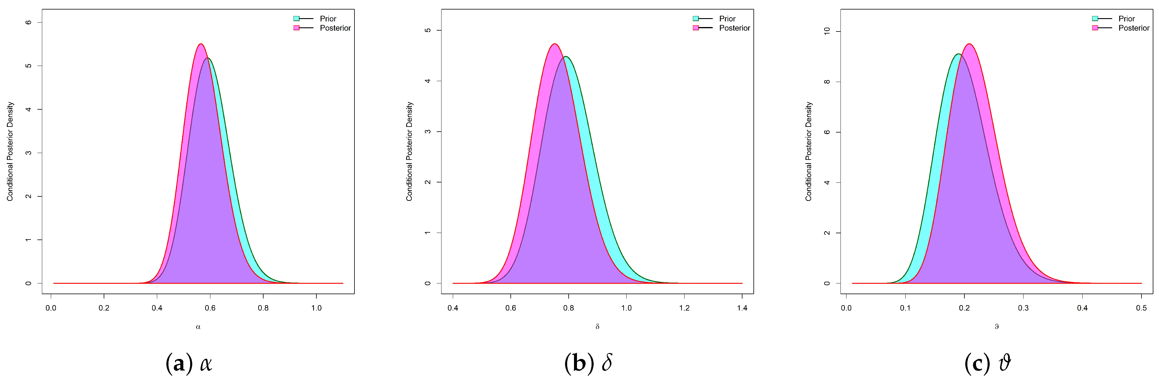
It is clear that the ratio of the integrals in (13) cannot be evaluated in closed form. Therefore, MCMC techniques are employed to obtain the corresponding objective Bayes estimates. By simulating a random sample under the proposed censoring design from $\mathrm{APW}(0.5,0.8,0.2)$ with $(n,m)=(80,40)$, $(T_1,T_2)=(1,3)$, and $R_i=1$ for $i=1,2,\dots ,m$, Figure 2 shows that the posterior samples of $\alpha$, $\delta$, and $\vartheta$ generated from (14), (15), and (16) closely follow the Gaussian distribution. Thus, the Metropolis–Hastings (MH) method based on the normal proposal density is recommended for solving this issue; see, for details Gelman et al. [16]. The MH algorithm’s steps are provided in Algorithm 2.

Figure 2. The normal proposal and posterior density curves of $\alpha$, $\delta$, and $\vartheta$.

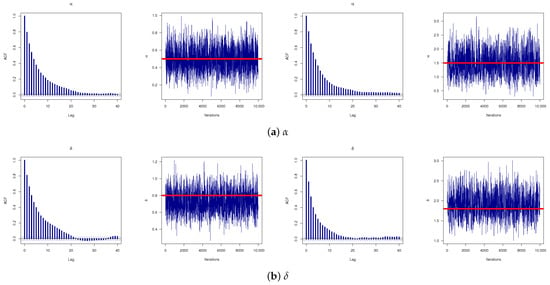
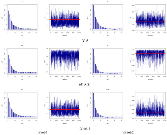
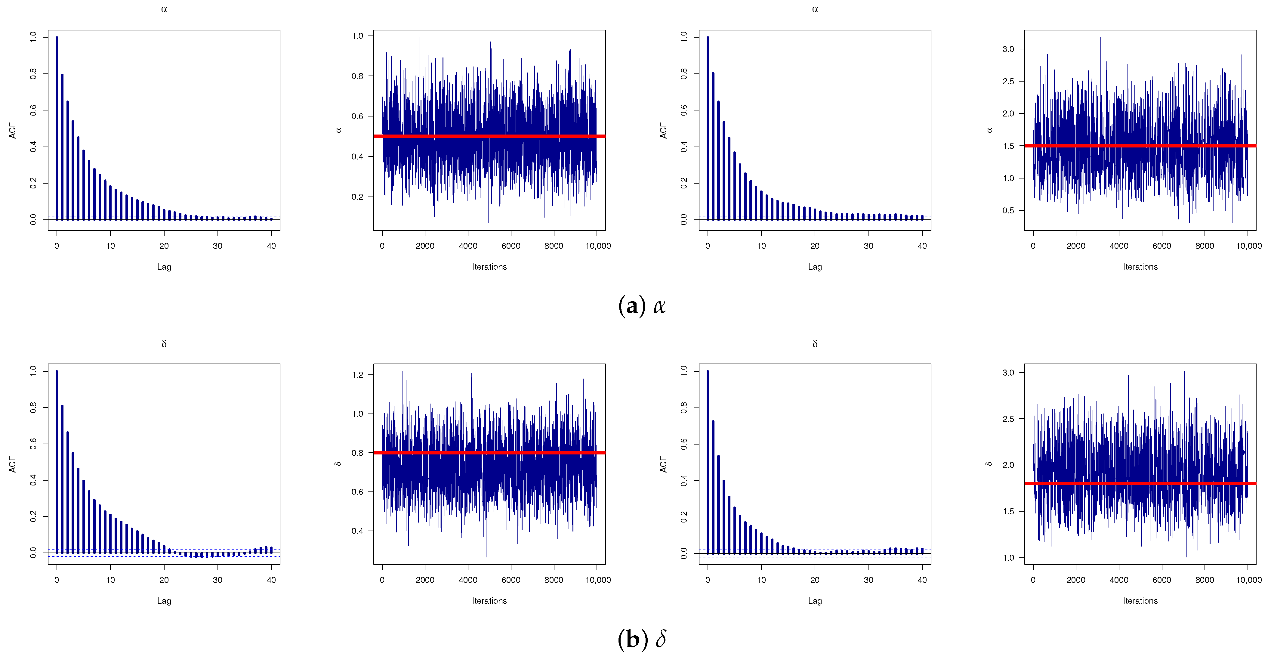
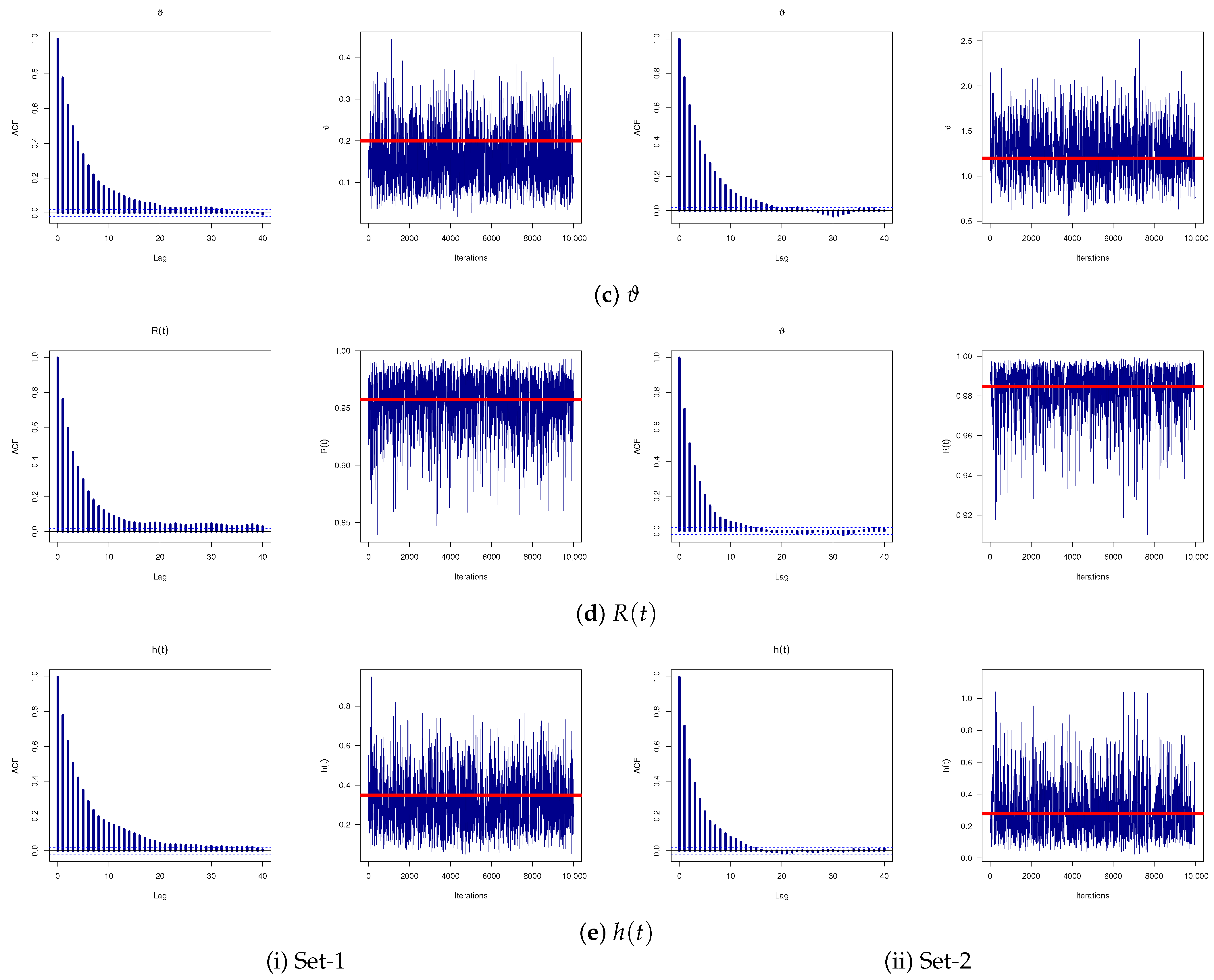
By simulating 12,000 MCMC variates and ignoring the first 2000 as burn-in from each unknown subject, based on the same proposed censoring values used to carry out Figure 2, two convergence diagnoses called autocorrelation function (ACF) and trace plots of $\alpha$, $\delta$, $\vartheta$, $R\left(t\right)$, and $h\left(t\right)$ are shown in Figure 3. It shows that the remaining 10,000 Markov chain draws of $\alpha$, $\delta$, $\vartheta$, $R\left(t\right)$, and $h\left(t\right)$ have converged superiority, and thus, the calculated estimates are stable and efficient. For clarity, the horizontal red line in each trace plot represents the proposed true value of each parameter considered.

Algorithm 2 The MH Sampling for $\alpha$, $\delta$, and $\vartheta$

1: Input: Set $\alpha =\widehat{\alpha },\delta =\widehat{\delta },\mathrm{a}\mathrm{n}\mathrm{d}\widehat{\vartheta }=\vartheta$   2: Input: Set $i\leftarrow 1$   3: Initialize: ${\alpha }^{*}\leftarrow \widehat{\alpha }$, ${\delta }^{*}\leftarrow \widehat{\delta }$, ${\vartheta }^{*}\leftarrow \widehat{\vartheta }$   4: for $i=1$ to $\mathcal{H}$ do   5:     Generate ${\alpha }^{\circ }\sim N(\widehat{\alpha },{\widehat{v}}_{\widehat{\alpha }\widehat{\alpha }})$   6:     Compute ${\xi }_{\alpha }=min\left\{1,{\displaystyle \frac{{\mathcal{P}}_{\tau }^{\alpha }({\alpha }^{\circ }\mid \mathbf{x})}{{\mathcal{P}}_{\tau }^{\alpha }({\alpha }^{(i-1)}\mid \mathbf{x})}}\right\}$   7:     Generate $u\sim U(0,1)$   8:     if $u<{\xi }_{\alpha }$ then   9:         Set ${\alpha }^i\leftarrow {\alpha }^{\circ }$ 10:     else 11:         ${\alpha }^i\leftarrow {\alpha }^{i-1}$ 12:     end if 13:     Redo Steps 4–12 for $\delta$ and $\vartheta$ 14:     Compute $$\begin{array}{cc}\hfill R^i\left(t\right)& ={\displaystyle \frac{{\alpha }^i}{{\alpha }^i-1}}\left(1-{\alpha }^{i^{-\exp \left(-{\vartheta }^i{t}^{{\delta }^i}\right)}}\right),\hfill \\ h^i\left(t\right)& \hfill ={\displaystyle \frac{{\vartheta }^i{\delta }^i\log \left({\alpha }^i\right)t^{{\delta }^i-1}\exp \left(-{\vartheta }^i{t}^{{\delta }^i}\right)}{{\alpha }^{i^{\exp \left(-{\vartheta }^i{t}^{{\delta }^i}\right)}}-1}}.\end{array}$$ 15: end for 16: Input: Burn-in $i^{★}$ 17: Output: ${\{{\alpha }^i,{\delta }^i,{\vartheta }^i,R^i\left(t\right),h^i\left(t\right)\}}_{i=i^{★}+1}^{\mathcal{H}}$

Figure 3. The ACF (left) and Trace (right) shapes of $\alpha$, $\delta$, $\vartheta$, $R\left(t\right)$ and $h\left(t\right)$.

4. Interval Inference

This section presents the construction of ACI estimators, derived from the observed FI, and BCI/HPD interval estimators, obtained via MCMC-generated posterior samples, for the parameters $\alpha$, $\delta$, and $\vartheta$, and the reliability measures $R\left(t\right)$ and $h\left(t\right)$.

4.1. Asymptotic Intervals

To create the ACIs for $\delta$ and $\theta$, first establish the asymptotic variance-covariance (AVC) matrix, which is the inverse of the Fisher information data matrix. Under conventional regularity assumptions, the MLEs ($\widehat{\alpha },\widehat{\delta },\widehat{\vartheta }$) are roughly multivariate normally distributed, with a mean vector $\left(\mathit{\theta }\right)$ and an AVC matrix ${\mathbf{I}}^{-1}\left(\mathit{\theta }\right)$.

Following Lawless [17], ${\mathbf{I}}^{-1}\left(\mathit{\theta }\right)$ is estimated by ${\mathbf{I}}^{-1}\left(\widehat{\mathit{\theta }}\right)$ through substitution of the MLEs $\widehat{\alpha }$, $\widehat{\delta }$, and $\widehat{\vartheta }$ in the place of $\alpha$, $\delta$, and $\vartheta$, respectively. The

$$\begin{array}{cc}\hfill {\mathbf{I}}_{3\times 3}^{-1}(\widehat{\mathit{\theta }})& \cong {\left[\begin{array}{c}-{\mathcal{L}}_{11}-{\mathcal{L}}_{12}-{\mathcal{L}}_{13}\\ -{\mathcal{L}}_{21}-{\mathcal{L}}_{22}-{\mathcal{L}}_{23}\\ -{\mathcal{L}}_{31}-{\mathcal{L}}_{32}-{\mathcal{L}}_{33}\end{array}\right]}_{(\widehat{\alpha },\widehat{\delta },\widehat{\vartheta })}^{-1}\hfill \\ \hfill & =\left[\begin{array}{c}{\widehat{v}}_{\widehat{\alpha }\widehat{\alpha }}{\widehat{v}}_{\widehat{\alpha }\widehat{\delta }}{\widehat{v}}_{\widehat{\alpha }\widehat{\vartheta }}\\ {\widehat{v}}_{\widehat{\delta }\widehat{\alpha }}{\widehat{v}}_{\widehat{\delta }\widehat{\delta }}{\widehat{v}}_{\widehat{\delta }\widehat{\vartheta }}\\ {\widehat{v}}_{\widehat{\vartheta }\widehat{\alpha }}{\widehat{v}}_{\widehat{\vartheta }\widehat{\delta }}{\widehat{v}}_{\widehat{\vartheta }\widehat{\vartheta }}\end{array}\right],\hfill \end{array}$$

(17)

where ${\mathcal{L}}_{ij}$ for $i,j=1,2,3,$ are obtained and presented in Appendix A.

Accordingly, the two-sided $100(1-\sigma )\%$ ACI estimators using the normality approximation (NA) method (denoted by ACI-NA) for $\alpha$, $\delta$, and $\vartheta$ are respectively given by

$$\widehat{\alpha }\pm z_{{\displaystyle \frac{\sigma }{2}}}\sqrt{{\widehat{v}}_{\widehat{\alpha }\widehat{\alpha }}},\widehat{\delta }\pm z_{{\displaystyle \frac{\sigma }{2}}}\sqrt{{\widehat{v}}_{\widehat{\delta }\widehat{\delta }}},\mathrm{and}\widehat{\vartheta }\pm z_{{\displaystyle \frac{\sigma }{2}}}\sqrt{{\widehat{v}}_{\widehat{\vartheta }\widehat{\vartheta }}},$$

where $z_{{\displaystyle \frac{\sigma }{2}}}$ represents the upper ${\displaystyle \frac{\sigma }{2}}$ quantile of the standard normal distribution.

Additionally, to develop the $100(1-\sigma )\%$ ACI-NA estimators for $R\left(t\right)$ and $h\left(t\right)$ (for $t>0$), their respective approximate variances, denoted by ${\widehat{v}}_{\widehat{R}}$ and ${\widehat{v}}_{\widehat{h}}$, must first be evaluated. So, the delta method is employed to first obtain the estimated variances of $\widehat{R}\left(t\right)$ and $\widehat{h}\left(t\right)$ (see Greene [18]), after which the ACI-NA estimators of $R\left(t\right)$ and $h\left(t\right)$ are constructed as

$${\widehat{v}}_{\widehat{R}}^2={\mathrm{\Lambda }}_{\widehat{R}}^{\mathsf{T}}{\mathbf{I}}^{-1}\left(\widehat{\mathit{\theta }}\right){\mathrm{\Lambda }}_{\widehat{R}}\mathrm{a}\mathrm{n}\mathrm{d}{\widehat{v}}_{\widehat{h}}^2={\mathrm{\Lambda }}_{\widehat{h}}^{\mathsf{T}}{\mathbf{I}}^{-1}\left(\widehat{\mathit{\theta }}\right){\mathrm{\Lambda }}_{\widehat{h}},$$

where, in Appendix B, the results of ${\mathrm{\Lambda }}_{\widehat{R}}$ and ${\mathrm{\Lambda }}_{\widehat{h}}$ are presented.

Following that, the two-sided $100(1-\sigma )\%$ ACI-NA estimators of $R\left(t\right)$ and $h\left(t\right)$ are provided by

$$\begin{array}{c}\hfill \widehat{R}\left(t\right)\pm z_{{\displaystyle \frac{\sigma }{2}}}\sqrt{{\widehat{v}}_{\widehat{R}}^2}\mathrm{a}\mathrm{n}\mathrm{d}\widehat{h}\left(t\right)\pm z_{{\displaystyle \frac{\gamma }{2}}}\sqrt{{\widehat{v}}_{\widehat{h}}^2}.\end{array}$$

respectively.

One notable drawback of the ACI-NA approach is that its lower confidence limit may occasionally be negative, which is implausible for lifetime or reliability parameters. To overcome this shortcoming, Meeker and Escobar [19] proposed the use of a normal transformation of the log-MLE $\alpha$, $\delta$, or $\vartheta$. They further showed that, compared to other normal-based interval estimation methods, the log-transformed (ACI-NL) tends to exhibit improved coverage accuracy. Therefore, the $100(1-\sigma )\%$ ACI-NL for $\alpha$ is given by

$$\widehat{\alpha }\exp \left(\mp z_{{\displaystyle \frac{\sigma }{2}}}{\widehat{\alpha }}^{-1}\sqrt{{\widehat{v}}_{\widehat{\alpha }\widehat{\alpha }}}\right),$$

where, similarly, the $100(1-\sigma )\%$ ACI-NL for $\delta$, $\vartheta$, $R\left(t\right)$, or $h\left(t\right)$ can be derived in an analogous manner.

4.2. Bayesian Intervals

In this part, the $(1-\sigma )100\%$ BCI and HPD bounds of $\alpha$, $\delta$, $\vartheta$, $R\left(t\right)$, and $h\left(t\right)$ are produced based on the MCMC samples generated by Algorithm 2. Specifically, Algorithm 3 provides a thorough technique for performing Bayesian interval setup.

Algorithm 3 The Bayesian Credible Sampling for $\alpha$, $\delta$, $\vartheta$, $R\left(t\right)$, and $h\left(t\right)$

1: Input: Confidence level $(1-\sigma )$ 2: Output: $(1-\sigma )100\%$ BCI and HPD intervals for $\alpha$, $\delta$, $\vartheta$, $R\left(t\right)$, and $h\left(t\right)$ 3: Sort the posterior samples ${\alpha }^{\left(i\right)}$, for $i={\varsigma }^{★}+1,\dots ,\mathcal{H}$, in ascending order. 4: Compute the $(1-\sigma )100\%$ BCI for $\alpha$ as: $$\left({\alpha }_{\left({\displaystyle \frac{\sigma }{2}}{\varsigma }^{★}\right)},{\alpha }_{\left(\left(1-{\displaystyle \frac{\sigma }{2}}\right){\varsigma }^{★}\right)}\right)$$ 5: Determine the $(1-\sigma )100\%$ HPD interval for $\alpha$ as: $$\left({\alpha }_{\left({\varsigma }^{★}\right)},{\alpha }_{({\varsigma }^{★}+(1-\sigma ){\varsigma }^{★})}\right)$$ where ${\varsigma }^{★}$ denotes the index that minimizes: $${\alpha }_{\left(\varsigma +(1-\sigma ){\varsigma }^{★}\right)}-{\alpha }_{\left(\varsigma \right)},\mathrm{for}\varsigma ={\varsigma }^{★}+1,\dots ,\mathcal{H}.$$ 6: Redo Steps 3–5 for $\delta$, $\vartheta$, $R\left(t\right)$, and $h\left(t\right)$ to obtain their respective BCI and HPD intervals.

5. Monte Carlo Simulations

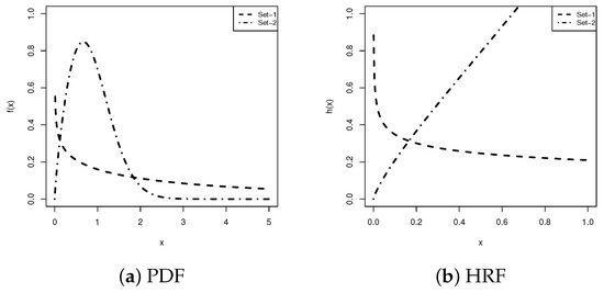
To show the efficiency of the proposed estimators for the parameters $\alpha$, $\delta$, and $\vartheta$, as well as for the reliability time metrics $R\left(t\right)$ and $h\left(t\right)$, we conducted an extensive Monte Carlo simulation study. A total of 1000 GTII-PHC samples were generated from two APW populations, namely Set–1: $(0.5,0.8,0.2)$ and Set–2: $(1.5,1.8,1.2)$. At $t=0.1$, the true reliability values are $(0.9572,0.3482)$ for Set–1 and $(0.9846,0.2728)$ for Set–2, corresponding to $R\left(t\right)$ and $h\left(t\right)$, respectively. To further clarify the rationale behind selecting sets 1 and 2 of the APW model, Figure 4 illustrates that the APW density displays decreasing and right-skewed distributions, respectively. It also indicates, for sets 1 and 2, that the APW failure rate provides decreasing and increasing patterns, respectively. These features indicate that the various simulation settings proposed are, in turn, made to cover the typical life distribution patterns of the proposed model.

Figure 4. The PDF and HRF shapes of the APW model from Set–$i,i=1,2$.

The simulation design aimed to explore the impact of varying experimental conditions, including the choice of threshold times $T_i,i=1,2$, the sample size n, the effective sample size m, and the censoring scheme $\mathbf{R}$. For both populations, the threshold pairs $(T_1,T_2)$ were set to $(0.5,1.5)$ and $(1.5,2.5)$, while three levels of n were considered: 30, 50, and 80. Table 2 summarizes several censoring schemes $\mathbf{R}$. For example, the notation $1^2$ denotes that a single unit is censored at each of the first and second stages. The censoring plans CS-i (for $i=1,2,3$) in Table 2, in practice, are analogous to left-, middle-, and right-censoring, respectively.

Table 2. Several CSs of $\mathbf{R}$ in Monte Carlo comparisons.

Test	$\mathit{R}=({\mathit{R}}_1,{\mathit{R}}_2,\dots ,{\mathit{R}}_{\mathit{m}})$
$(n,m)\to$	(30, 10)	(30, 20)
CS-1	$(5^4,0^6)$	$(5^2,0^{18})$
CS-2	$(0^3,5^4,0^3)$	$(0^9,5^2,0^9)$
CS-3	$(0^6,5^4)$	$(0^{18},5^2)$
$(n,m)\to$	(50, 20)	(50, 40)
CS-1	$(5^6,0^{14})$	$(5^2,0^{38})$
CS-2	$(0^7,5^6,0^7)$	$(0^{19},5^2,0^{19})$
CS-3	$(0^{14},5^6)$	$(0^{38},5^2)$
$(n,m)\to$	(80, 30)	(80, 60)
CS-1	$(5^{10},0^{20})$	$(5^4,0^{56})$
CS-2	$(0^{10},5^{10},0^{10})$	$(0^{28},5^4,0^{28})$
CS-3	$(0^{20},5^{10})$	$(0^{56},5^4)$

After generating the required GTII-PHC samples using $\mathsf{R}$ (version 4.2.2), the unknown parameters $\alpha$, $\delta$, $\vartheta$, $R\left(t\right)$, and $h\left(t\right)$ were analyzed through two statistical packages:

(i)

The $\mathsf{maxLik}$ package, via the $\mathsf{maxNR}$ function (Henningsen and Toomet [20]), to compute the MLEs along with the corresponding ACIs through NA and NL approaches.

(ii)

The $\mathsf{coda}$ package (Plummer et al. [21]), to obtain posterior estimates and their BCI/HPD intervals through the proposed MCMC approach.

For the MH algorithm, the first 2000 of 12,000 iterations were discarded as burn-in, with the remaining samples used to derive Bayes–MCMC analysis of $\alpha$, $\delta$, $\vartheta$, $R\left(t\right)$, and $h\left(t\right)$. To assess prior sensitivity, two sets of hyperparameters $(a_i,b_i)$, $i=1,2,3$, were considered. Following Kundu [22], and using the mean–variance criterion in selecting gamma prior values, the hyperparameters $(a_i,b_i)$ for $i=1,2,3$ were assigned as:

• For Set–1:

  –

  Prior-A: $(a_1,a_2,a_3)=(2.5,4,1)$ and $b_i=5,i=1,2,3;$

  –

  Prior-B: $(a_1,a_2,a_3)=(5,8,2)$ and $b_i=10,i=1,2,3.$

• For Set–2:

  –

  Prior-A: $(a_1,a_2,a_3)=(7.5,9,6)$ and $b_i=5,i=1,2,3;$

  –

  Prior-B: $(a_1,a_2,a_3)=(15,18,12)$ and $b_i=10,i=1,2,3.$

Now, to further investigate the performance of the estimators of $\alpha$, $\delta$, $\vartheta$, $R\left(t\right)$, or $h\left(t\right)$ (say, $\rho$, for short), the respective root mean squared error (RMSE) and mean relative absolute bias (MRAB) can be calculated as follows:

$$\mathrm{RMSE}\left(\widehat{\rho }\right)=\sqrt{{\displaystyle \frac{1}{1000}}{\sum }_{j=1}^{1000}{\left({\widehat{\rho }}^{\left[j\right]}-\rho \right)}^2},\mathrm{MRAB}\left(\widehat{\rho }\right)={\displaystyle \frac{1}{1000}}{\sum }_{j=1}^{1000}{\rho }^{-1}\left|{\widehat{\rho }}^{\left[j\right]}-\rho \right|,$$

where ${\widehat{\rho }}^{\left[j\right]}$ represents the point estimate of $\rho$ from the jth replication.

In addition, the performance of the 95% intervals is evaluated using two criteria: average interval length (AIL) and coverage probability (CP), defined as follows:

$${\mathrm{AIL}}^{95\%}\left(\rho \right)={\displaystyle \frac{1}{1000}}{\sum }_{j=1}^{1000}\left(\mathsf{U}{\widehat{\rho }}^{\left[j\right]}-\mathsf{L}{\widehat{\rho }}^{\left[j\right]}\right),{\mathrm{CP}}^{95\%}\left(\rho \right)={\displaystyle \frac{1}{1000}}{\sum }_{j=1}^{1000}{\mathrm{\Psi }}^{★}\left(\mathsf{L}{\widehat{\rho }}^{\left[j\right]},\mathsf{U}{\widehat{\rho }}^{\left[j\right]}\right)\left(\rho \right),$$

where ${\mathrm{\Psi }}^{★}(·)$ denotes the indicator function, and $(\mathsf{L},\mathsf{U})$ represent the interval bounds.

Table A1, Table A2, Table A3, Table A4 and Table A5 report the point estimation results for $\alpha$, $\delta$, $\vartheta$, $R\left(t\right)$, and $h\left(t\right)$, while the corresponding interval estimation results are summarized in Table A5, Table A6, Table A7 and Table A8. For short, all Table A1, Table A2, Table A3, Table A4, Table A5, Table A6, Table A7, Table A8, Table A9 and Table A10 of $\alpha$, $\delta$, $\vartheta$, $R\left(t\right)$, and $h\left(t\right)$ are provided in Appendix C. Following the lowest RMSE, MRAB, and AIL values together with the highest CP values, several key observations are drawn:

• In general, the collected results of $\alpha$, $\delta$, and $\vartheta$, along with the reliability measures $R\left(t\right)$ and $h\left(t\right)$, exhibit strong performance, producing low RMSE, MRAB, and AIL values with consistently high CP values.
• Estimation quality improves with larger sample size n or effective sample size m, and likewise improves when the total of withdrawals in $\mathbf{R}$ decreases.
• For interval estimation, the lower bounds of all parameters remain strictly positive across simulations, and the estimated intervals for $R\left(t\right)$ consistently lie within $(0,1)$, in accordance with theoretical expectations.
• A comparison of CS-i (for $i=1,2,3$) reveals the following:

  –

  Estimators of $\alpha$, $\vartheta$, and $h\left(t\right)$ perform best under CS-3 (removal of $n-m$ units at the last stage);

  –

  Estimators of $\delta$ perform best under CS-2 (removal of $n-m$ units at the middle-stage).

  –

  Estimators of $R\left(t\right)$ perform best under CS-1 (removal of $n-m$ units at the firs-stage).

• When the parameter values of APW($\alpha ,\delta ,\vartheta$) increase, it is noted that:

  –

  Both RMSEs and MRABs of $\alpha$, $R\left(t\right)$, and $h\left(t\right)$ tend to decrease, while those of $\delta$ and $\vartheta$ tend to increase;

  –

  The AILs for all parameters and reliability indices increased, while the opposite fact was observed when comparing based on the CP results.

• A comparison between the two Bayesian estimators shows that Prior-B consistently outperforms Prior-A, achieving lower RMSE, MRAB, and AIL values, and higher CP values. This advantage is primarily due to the smaller prior variance associated with Prior-B than its competitor.
• Overall, the findings demonstrate that Bayesian MCMC inference via the M–H strategy provides the most reliable estimates for both parameters and reliability characteristics of the APW distribution under the proposed censored dataset.

6. Three Data Applications

This section presents three real-world applications, one each from engineering, clinical, and physical domains, to illustrate the practical utility of the proposed estimation methods and their relevance in real-life contexts. The analyses confirm that the recommended inferential procedures perform satisfactorily when applied to actual data under the proposed censoring schemes. The applications are outlined as follows:

• Engineering Application: In this application (say, App. 1), we shall analyze a real dataset consisting of the recorded failure times of eighteen electronic devices, providing valuable insights into their reliability and lifetime characteristics. Such data are essential for modeling, estimation, and assessing the performance of electronic components under real-world operating conditions; see Elshahhat and Abu El Azm [23].
• Clinical Application: In this application (say, App. 2), a total of 56 blood samples, collected from organ transplant recipients to assess post-transplant monitoring, will be analyzed. Each sample was developed using a standard approved method, high-performance liquid chromatography (HPLC), to ensure accurate and reliable quantification; see Hawkins [24] and Elshahhat et al. [25].
• Physical Application: In this application (say, App. 3), we examine a dataset comprising 25 diamond size measurements collected from a major mining region in Southwestern Africa, which represents valuable information on the variability of diamond sizes in this area. This set of data was originally provided by Maurya and Goyal [26]. Such data play an important role in statistical modeling and analysis, particularly for understanding distributional properties and supporting mining and economic decision-making.

To strengthen the practical relevance of the three real-data analyses, we provide additional background regarding the engineering and scientific settings from which these datasets originate, along with a brief justification of the APW model’s suitability. The first application, based on electronic device data, illustrates the model’s ability to capture reliability behavior and component wear-out patterns; the second application, based on post-transplant biomarker measurements, highlights its suitability for asymmetric biomedical and clinical monitoring scenarios; and the third application, based on the diamond size data, confirms its capacity to describe distributional variability in geological and mining contexts. Across all three cases, the combined use of the GTII-PHC scheme by the APW-based model provides interpretable parameters, robust estimation under partial observation, and direct engineering implications such as improved lifetime prediction and risk quantification for real experimental systems.

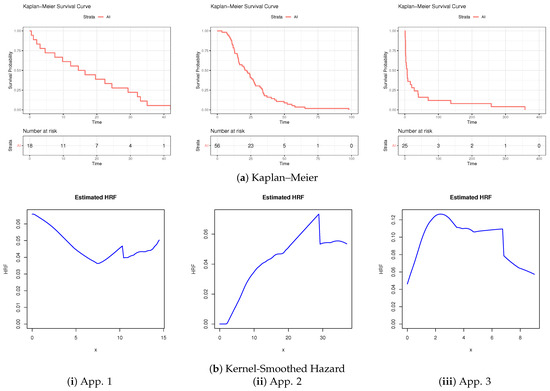
The use of Kaplan–Meier (KM) survival curves and kernel-smoothed HRF functions provides a powerful, nonparametric framework for uncovering the underlying reliability behavior of diverse lifetime datasets without imposing restrictive model assumptions. The KM estimates offer a clear view of the empirical survival structure, enabling direct comparison of failure patterns across the three applications, while kernel-smoothed hazard functions reveal the instantaneous risk dynamics, such as aging, burn-in, or early-life failures, that the survival curve alone cannot capture. Together, these complementary tools deliver a comprehensive diagnostic foundation that supports model validation; see Figure 5. It exhibits that:

Figure 5. The KM estimate and kernel-based hazard rate diagnostic curves for the three science datasets.

• The KM curve shows a sharp early decline in survival, indicating substantial early-life failures. The kernel-smoothed hazard exhibits an early peak followed by a decline, confirming an infant-mortality effect and a bathtub-shaped failure pattern.
• The KM curve decreases gradually over time, reflecting steady accumulation of failures rather than early clustering. The monotonically increasing hazard function indicates a dominant aging and wear-out mechanism.
• The KM curve maintains high early survival with slower initial failure accumulation. The decreasing hazard rate confirms a burn-in effect, where reliability improves after early weak units fail.

Across all considered applications, the combined KM and kernel-smoothed HRF diagnostics effectively discriminate among distinct failure regimes—infant mortality (App. 1), aging wear-out (App. 2), and burn-in reliability improvement (App. 3). This complementary interpretation provides a robust empirical validation of the proposed APW modeling assumptions and confirms that the datasets represent fundamentally different reliability mechanisms, not merely differences in size.

For computational issues, each original data point reported in Applications 1 and 2 has been rescaled by dividing by ten; see Table 3. Before proceeding with further analysis of the acquired estimates of $\alpha$, $\delta$, $\vartheta$, $R\left(t\right)$, and $h\left(t\right)$, we validate the APW distribution by estimating the parameters $\alpha$, $\delta$, and $\vartheta$ using the ML method for the datasets in Table 3. The corresponding MLEs, along with their standard errors (Std.Es) and 95% ACI-NA/ACI-NL estimates with interval widths (Int.Ls), are reported in Table 4, together with the Kolmogorov–Smirnov (KS) statistic and its associated p-value. These results confirm that the APW distribution provides an adequate fit to the datasets of the three sciences considered.

Table 3. Different failure times of three sciences.

Data	Times
App. 1	0.5	1.1	2.1	3.1	4.6	7.5	9.8	12.2	14.5	16.5
	19.6	22.4	24.5	29.3	32.1	33	35	42
App. 2	3.5	7.1	7.7	8.7	9.3	9.9	10.4	10.9	10.9	11.2
	11.8	11.8	12.5	12.7	12.9	13	14.8	15.1	15.3	15.6
	15.9	15.9	16.2	16.6	18.5	19.8	20.3	20.6	22.1	22.7
	24.1	24.4	24.5	25.4	26.6	27.1	27.5	28	28.5	31.8
	32.7	33.6	33.9	34	34.6	35	37	40.2	42.8	44
	49.8	52.1	55.6	57.8	65.3	98
App. 3	1	1	1.5	2	2	2	2	2.5	3	3
	4.5	5	7	7	7.5	9	16.5	20.5	28	39
	40.5	69.5	137	257.5	358

Table 4. Summary fit of the APW model from three sciences.

Data	Par.	MLE (Std.E)	95% ACI-NA			95% ACI-NL			KS (p-Value)
			Low.	Upp.	Int.L	Low.	Upp.	Int.L
App. 1	$\alpha$	219.33 (52.545)	116.34	322.32	205.97	137.14	350.77	213.62	0.1085 (0.9684)
	$\delta$	0.6210 (0.1215)	0.3829	0.8592	0.4763	0.4232	0.9113	0.4881
	$\vartheta$	0.3932 (0.1554)	0.0886	0.6978	0.6092	0.1812	0.8532	0.6720
App. 2	$\alpha$	539.13 (71.319)	399.34	678.91	279.56	415.99	698.70	282.71	0.0865 (0.7957)
	$\delta$	0.7832 (0.0840)	0.6186	0.9477	0.3292	0.6347	0.9663	0.3316
	$\vartheta$	0.2013 (0.0579)	0.0878	0.3149	0.2273	0.1145	0.3540	0.2395
App. 3	$\alpha$	303.67 (60.562)	184.98	422.38	237.40	205.43	448.92	243.49	0.1548 (0.5869)
	$\delta$	0.3373 (0.0463)	0.2466	0.4282	0.1815	0.2578	0.4415	0.1837
	$\vartheta$	0.9686 (0.1745)	0.6266	1.3107	0.6841	0.6805	1.3789	0.6984

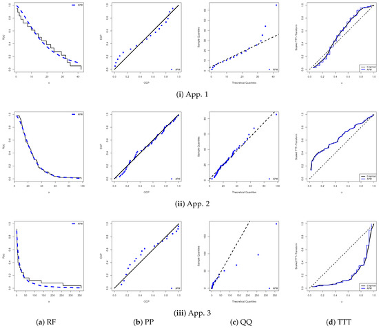
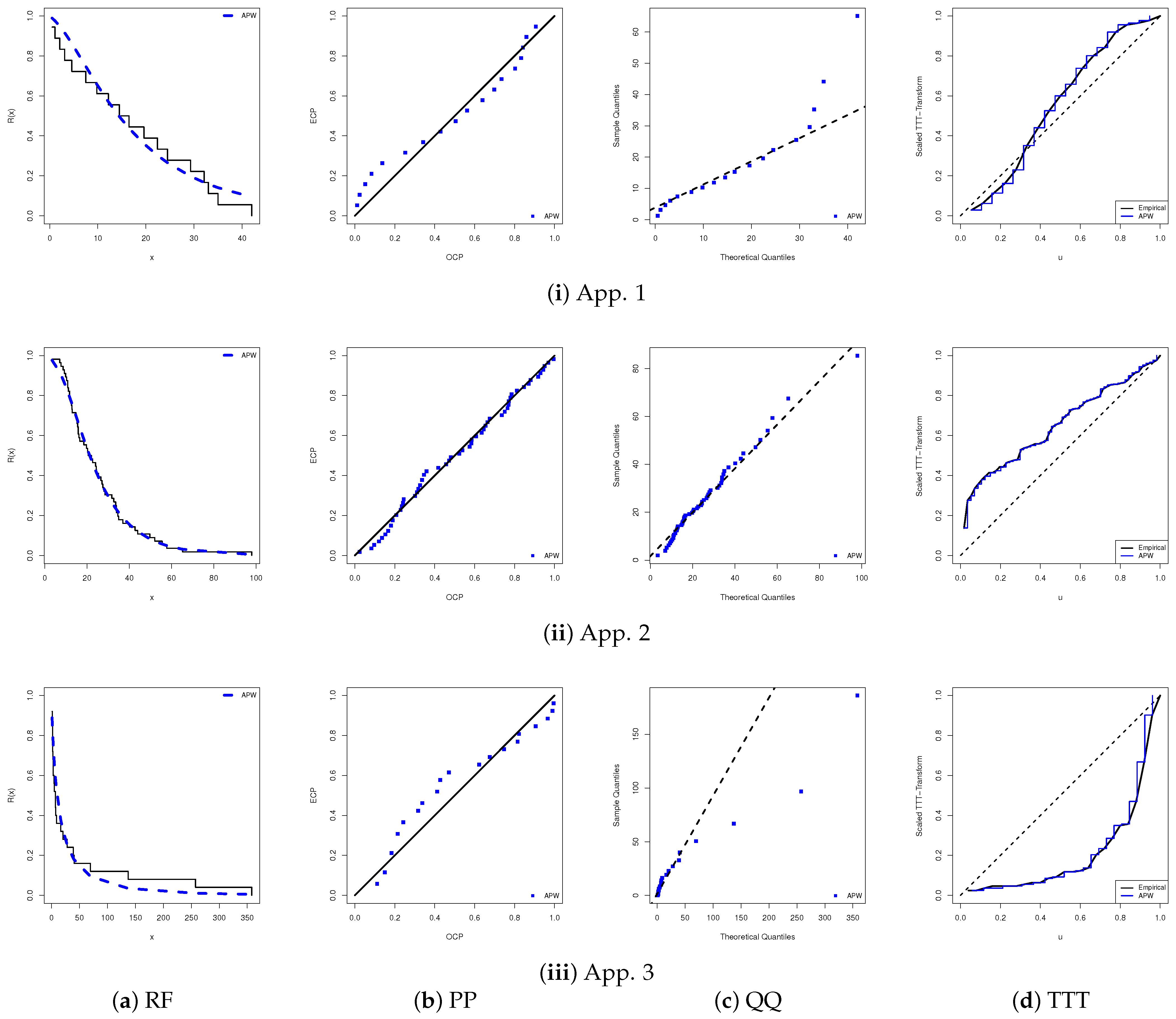
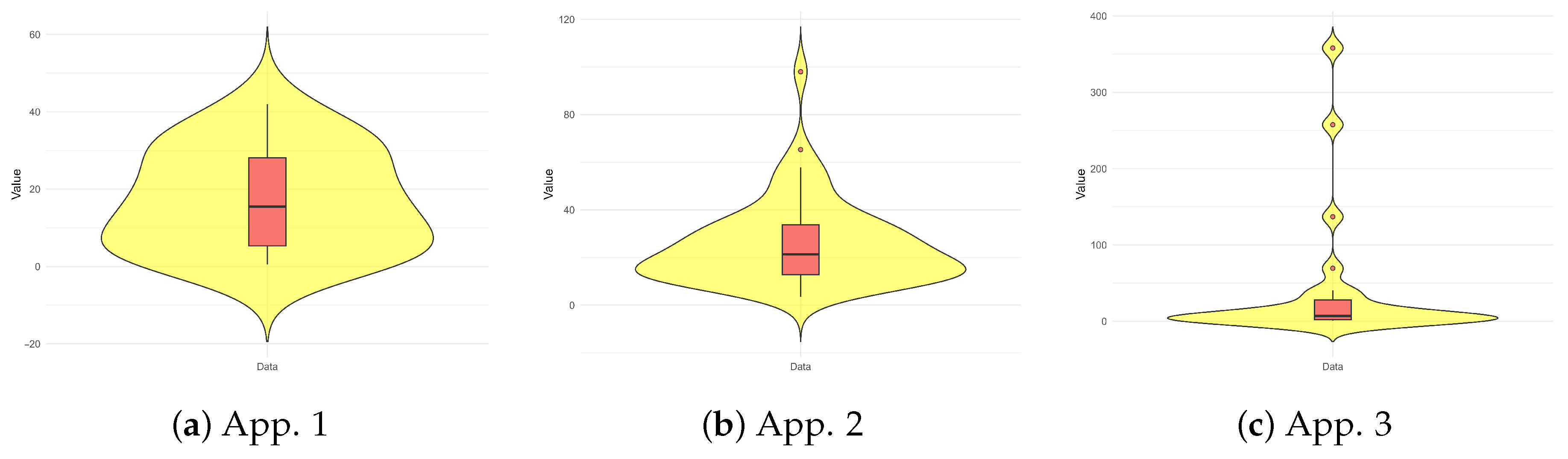
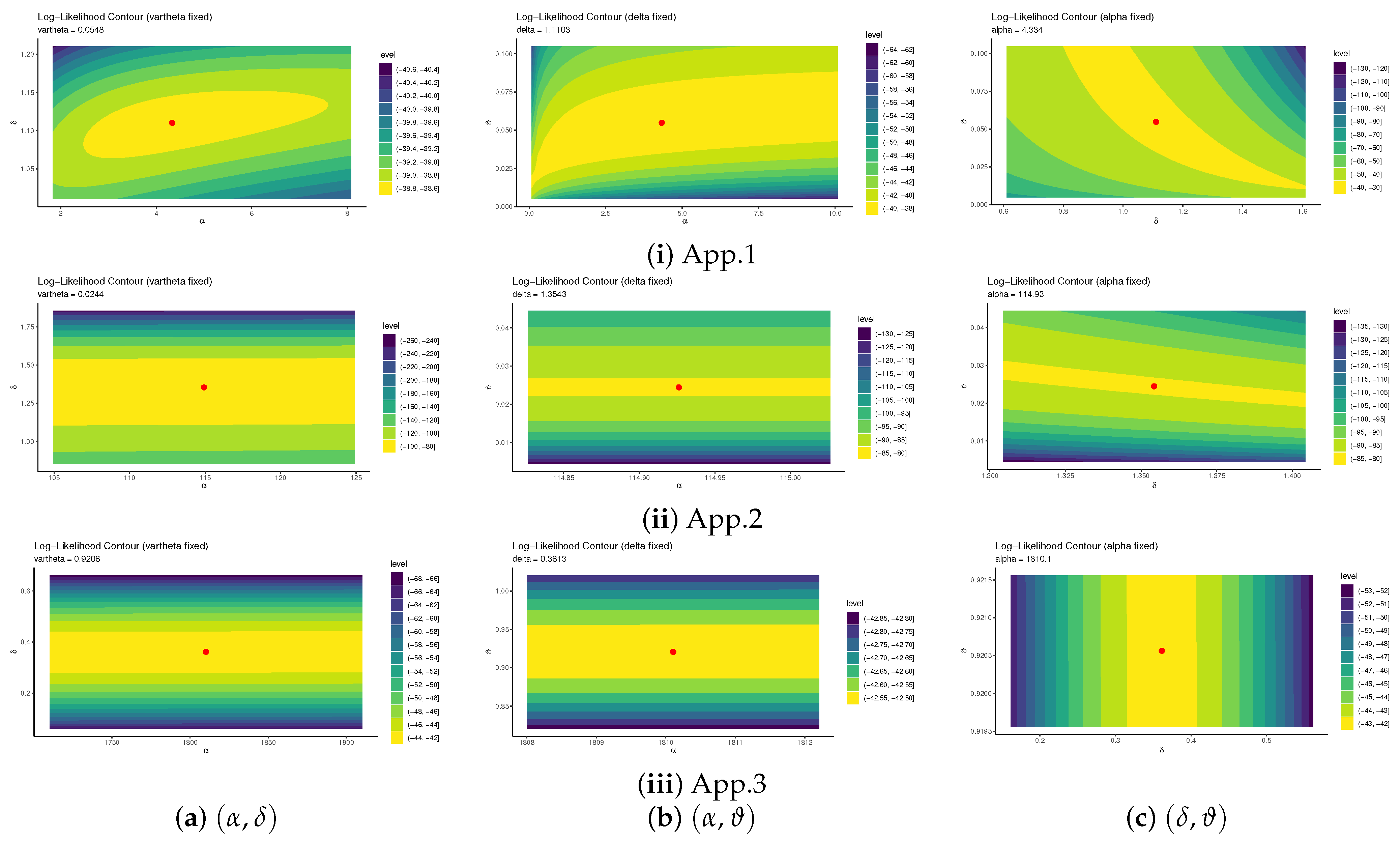
To complement the numerical findings, Figure 6 displays six diagnostic plots of the APW model: (a) empirical versus fitted reliability plots, (b) PP plots, (c) QQ plots, and (d) scaled-TTT plots. The diagnostics in Figure 6a–c support the numerical results in Table 4. Moreover, Figure 6d indicates that the associated datasets in App. i (for $i=1,2,3$) exhibit bathtub-shaped, increasing, and decreasing failure rates, respectively. It is worth noting here that all HRF curves in Figure 6d are consistent with theoretical APW failure rates. Figure 7 shows that the violin plot in Figure 7a shows a roughly symmetric distribution centered around the median, with moderate spread and no extreme outliers; Figure 7b indicates a slightly right-skewed distribution with a few noticeable outliers on the upper tail; and Figure 7c reveals a highly skewed distribution with several extreme high-value outliers, while most observations are concentrated near the lower end. Finally, the contour plots in Figure 8 confirm the existence and uniqueness of the MLEs of $\alpha$, $\delta$, and $\vartheta$ obtained from all given datasets, see Table 4. Accordingly, the fitted values $\widehat{\alpha }$, $\widehat{\delta }$, and $\widehat{\vartheta }$ are adopted as initial values for subsequent analyses.

Figure 6. Fitting diagrams for the APW model from three sciences.

Figure 7. Contours for the APW log-likelihood from three sciences.

Figure 8. Violin diagrams for the APW model from three sciences.

Briefly, to demonstrate the practical utility of the proposed APW model, we compare its goodness-of-fit performance with three well-known lifetime distributions that offer flexible or discrete failure-rate shapes, namely the exponentiated–Weibull (EW$(\alpha ,\delta ,\vartheta )$) distribution of Mudholkar and Srivastava [27], the Weibull–exponential (WE$(\alpha ,\delta ,\vartheta )$) distribution of Oguntunde et al. [28], and the Weibull (W$(\delta ,\vartheta )$) distribution of Weibull [29]. In addition to the $KS$(p-value) statistic, the comparative assessment relies on several model-selection criteria, including: (i) negative log-likelihood (NLL), (ii) Akaike information criterion (AIC), (iii) consistent AIC (CAIC), (iv) Bayesian information criterion (BIC), and (v) Hannan–Quinn information criterion (HQIC); see Table 5. The results reveal that the APW model achieves the smallest values of AIC, CAIC, BIC, HQIC, and $\mathsf{KS}$, along with the largest $\mathsf{P}$-value when compared with the W model (App. 1) and with both the W and WE models (Apps. 2 and 3). Furthermore, the proposed EW model exhibits superior fit across all competing distributions and emerges as the most appropriate choice for the considered datasets.

Table 5. Fitting outcomes of the APW model from three sciences.

App.	Model	NLL	AIC	CAIC	BIC	HQIC	KS (p-Value)
App. 1	APW	68.309	141.36	142.56	143.43	141.60	0.1085 (0.9684)
	EW	66.834	139.67	141.38	142.34	140.04	0.0783 (0.9994)
	WE	67.310	140.62	142.33	143.29	140.99	0.0894 (0.9961)
	W	68.999	142.00	142.80	143.78	142.24	0.1133 (0.9546)
App. 2	APW	226.49	458.54	458.10	464.61	460.89	0.0865 (0.7957)
	EW	224.28	454.55	455.01	460.63	456.91	0.0755 (0.9072)
	WE	229.23	464.46	464.92	470.53	466.81	0.0935 (0.7123)
	W	227.85	459.70	459.93	463.76	461.27	0.0908 (0.7445)
App. 3	APW	104.74	213.85	214.19	216.87	214.76	0.1548 (0.5869)
	EW	102.88	211.76	212.90	215.41	212.77	0.1411 (0.7019)
	WE	107.09	220.18	221.33	223.84	221.20	0.1873 (0.3442)
	W	106.59	217.19	217.74	219.63	217.87	0.1812 (0.3842)

To examine the theoretical properties of the estimators for $\alpha$, $\delta$, $\vartheta$, $R\left(t\right)$, and $h\left(t\right)$ derived earlier, GTII-PHC samples were generated with $m=20$ for App. 2 and $m=10$ for App. i ($i=1,2$), under various choices of $T_i$ ($i=1,2$) and censoring schemes $\mathbf{R}$ (see Table 6), based on the three datasets in Table 3. Since no prior information on the APW parameters was available, Bayesian estimation was carried out via an MCMC sampler with improper gamma priors ($a_i=b_i=0$, $i=1,2,3$). A total of 40,000 MCMC iterations were produced using the MH algorithm, discarding the first 10,000 as burn-in. From Table 3, both maximum likelihood and Bayesian estimates of $\alpha$, $\delta$, $\vartheta$, $R\left(t\right)$, and $h\left(t\right)$ (at $t=1$) were obtained, along with two-sided 95% ACI-NA/ACI-NL and BCI/HPD interval estimates.

Table 6. Different GTII-PHC samples from three sciences.

Data	Sample	R	${\mathit{T}}_1\left({\mathit{j}}_1\right)$	${\mathit{T}}_2\left({\mathit{j}}_2\right)$	${\mathcal{R}}^{•}$	${\mathcal{T}}^{•}$	Censored Times
App. 1	$\mathcal{S}\left[A\right]$	$(2^4,0^6)$	30(8)	40(10)	0	35	0.5	2.1	3.1	9.8	14.5	16.5	19.6	24.5	32.1	35
	$\mathcal{S}\left[B\right]$	$(0^3,2^4,0^3)$	10(5)	25(8)	2	25	0.5	1.1	2.1	3.1	7.5	12.2	19.6	24.5
	$\mathcal{S}\left[C\right]$	$(0^6,2^4)$	30(11)	35(11)	1	30	0.5	1.1	2.1	3.1	4.6	7.5	9.8	14.5	19.6	24.5	29.3
App. 2	$\mathcal{S}\left[A\right]$	$(3^{12},0^8)$	20(11)	55(20)	0	52.1	3.5	7.7	8.7	12.5	12.9	13	14.8	15.3	16.2	16.6
							19.8	20.3	26.6	27.1	27.5	28.5	33.6	34	42.8	52.1
	$\mathcal{S}\left[B\right]$	$(0^4,3^{12},0^4)$	30(14)	45(18)	2	45	3.5	7.1	7.7	8.7	9.3	11.8	12.9	15.6	20.6	22.7
							24.4	25.4	27.1	28	31.8	33.6	40.2	42.8
	$\mathcal{S}\left[C\right]$	$(0^8,3^{12})$	50(22)	60(22)	1	50	3.5	7.1	7.7	8.7	9.3	9.9	10.4	10.9	10.9	11.2	12.7
							14.8	15.1	16.6	22.1	24.4	28.5	33.9	35	37	40.2	49.8
App. 3	$\mathcal{S}\left[A\right]$	$(3^5,0^5)$	50(9)	140(10)	0	137	1	1.5	2	3	5	9	20.5	28	40.5	137
	$\mathcal{S}\left[B\right]$	$(0^2,3^5,0^3)$	10(6)	30(8)	2	30	1	1	1.5	2.5	4.5	7	16	28
	$\mathcal{S}\left[C\right]$	$(0^5,3^5)$	30(11)	50(11)	2	30	1	1	1.5	2	2	2	3	5	7.5	20	28

Table 7 presents the point estimates with their Std.E values and the corresponding interval estimates with Int.L values. The results show that the frequentist and Bayesian estimates are generally close, as expected. However, Table 7 highlights that Bayesian MCMC estimation achieves superior accuracy, providing more precise point estimates than ML. Moreover, while the asymptotic intervals based on the NA and NL methods are nearly identical, the BCI and HPD intervals are consistently shorter, demonstrating greater efficiency. Overall, the findings confirm that Bayes MCMC estimation via the MH algorithm outperforms its likelihood-based counterparts.

Table 7. Estimates of $\alpha$, $\delta$, $\vartheta$, $R\left(t\right)$, and $h\left(t\right)$ from three sciences.

Data	Sample	Par.	MLE		MCMC		ACI-NA			BCI
							ACI-NL			HPD
			Est.	Std.E	Est.	Std.E	Low.	Upp.	Int.L	Low.	Upp.	Int.L
App. 1	$\mathcal{S}\left[A\right]$	$\alpha$	4.33402	9.47173	4.33391	0.00578	0.00000	22.8983	22.8983	4.31434	4.35340	0.03906
							0.05979	314.152	314.093	4.31475	4.35373	0.03898
		$\delta$	1.11032	0.39813	1.11015	0.00572	0.33001	1.89063	1.56063	1.09090	1.12963	0.03873
							0.54984	2.24214	1.69230	1.09094	1.12967	0.03872
		$\vartheta$	0.05483	0.08547	0.05520	0.00472	0.00000	0.22235	0.22235	0.03940	0.07166	0.03226
							0.00258	1.16366	1.16107	0.03896	0.07107	0.03211
		$R\left(t\right)$	0.94099	0.01251	0.98868	0.00098	0.91648	0.96550	0.04903	0.98526	0.99195	0.00669
							0.91679	0.96583	0.04903	0.98542	0.99208	0.00666
		$h\left(t\right)$	0.70013	0.02230	0.02556	0.00223	0.65643	0.74383	0.08740	0.01813	0.03337	0.01524
							0.65776	0.74522	0.08746	0.01795	0.03313	0.01519
	$\mathcal{S}\left[B\right]$	$\alpha$	1.82652	8.29358	1.82643	0.00578	0.00000	18.0816	18.0816	1.80678	1.84607	0.03929
							0.00025	13385.4	13385.4	1.80708	1.84628	0.03919
		$\delta$	0.81631	0.40704	0.81614	0.00573	0.01852	1.61409	1.59557	0.79690	0.83585	0.03895
							0.30719	2.16918	1.86198	0.79677	0.83562	0.03885
		$\vartheta$	0.07957	0.19959	0.07966	0.00540	0.00000	0.47077	0.47077	0.06137	0.09817	0.03680
							0.00058	10.8614	10.8608	0.06155	0.09826	0.03671
		$R\left(t\right)$	0.94099	0.03067	0.96733	0.00220	0.88087	0.99111	0.11023	0.95979	0.97480	0.01501
							0.88275	1.00307	0.12031	0.95989	0.97488	0.01499
		$h\left(t\right)$	0.70013	0.03666	0.05463	0.00375	0.62827	0.77198	0.14371	0.04201	0.06753	0.02551
							0.63183	0.77580	0.14397	0.04184	0.06730	0.02546
	$\mathcal{S}\left[C\right]$	$\alpha$	2.03537	7.03009	2.03528	0.00577	0.00000	15.8141	15.8141	2.01564	2.05487	0.03923
							0.00234	1772.79	1772.79	2.01595	2.05511	0.03916
		$\delta$	0.85195	0.36764	0.85176	0.00573	0.13138	1.57251	1.44113	0.83254	0.87136	0.03882
							0.36567	1.98487	1.61920	0.83251	0.87128	0.03877
		$\vartheta$	0.07524	0.15227	0.07541	0.00521	0.00000	0.37368	0.37368	0.05785	0.09337	0.03551
							0.00142	3.97373	3.97230	0.05830	0.09377	0.03547
		$R\left(t\right)$	0.94099	0.02577	0.97150	0.00196	0.89048	0.99150	0.10103	0.96474	0.97813	0.01339
							0.89181	0.99288	0.10108	0.96473	0.97809	0.01336
		$h\left(t\right)$	0.70013	0.03219	0.04966	0.00348	0.63703	0.76322	0.12618	0.03800	0.06165	0.02365
							0.63979	0.76615	0.12635	0.03809	0.06173	0.02364
App. 2	$\mathcal{S}\left[A\right]$	$\alpha$	114.926	5.94353	114.926	0.00575	103.277	126.575	23.2982	114.907	114.946	0.03922
							103.848	127.186	23.33813	114.906	114.945	0.03913
		$\delta$	1.35430	0.21798	1.35389	0.00572	0.92707	1.78153	0.85445	1.33443	1.37324	0.03882
							0.98790	1.85660	0.86870	1.33398	1.37265	0.03867
		$\vartheta$	0.02443	0.01730	0.02468	0.00173	0.00000	0.05834	0.05834	0.01909	0.03084	0.01175
							0.00610	0.09787	0.09178	0.01903	0.03076	0.01173
		$R\left(t\right)$	0.94099	0.00035	0.99959	0.00003	0.94030	0.94168	0.00138	0.99948	0.99969	0.00020
							0.94030	0.94168	0.00138	0.99948	0.99969	0.00020
		$h\left(t\right)$	0.70013	0.00081	0.00113	0.00008	0.69853	0.70172	0.00319	0.00087	0.00142	0.00056
							0.69853	0.70172	0.00319	0.00086	0.00142	0.00056
	$\mathcal{S}\left[B\right]$	$\alpha$	4.93596	8.52816	4.93630	0.00595	0.00000	21.6509	21.6509	4.91567	4.95767	0.04199
							0.16699	145.896	145.729	4.91660	4.95785	0.04125
		$\delta$	1.70514	0.51658	1.70453	0.00553	0.69267	2.71761	2.02494	1.68589	1.72350	0.03760
							0.94164	3.08769	2.14604	1.68592	1.72350	0.03757
		$\vartheta$	0.00255	0.00556	0.00261	0.00029	0.00000	0.01344	0.01344	0.00167	0.00363	0.00195
							0.00004	0.18192	0.18189	0.00170	0.00364	0.00195
		$R\left(t\right)$	0.94099	0.00056	0.99968	0.00004	0.93990	0.94208	0.00219	0.99955	0.99979	0.00025
							0.93990	0.94208	0.00219	0.99955	0.99979	0.00024
		$h\left(t\right)$	0.70013	0.00159	0.00111	0.00012	0.69701	0.70324	0.00623	0.00071	0.00154	0.00083
							0.69702	0.70325	0.00623	0.00071	0.00154	0.00083
	$\mathcal{S}\left[C\right]$	$\alpha$	0.79640	1.92088	0.79646	0.00116	0.00000	4.56126	4.56126	0.79245	0.80050	0.00804
							0.00705	89.9892	89.9821	0.79233	0.80025	0.00793
		$\delta$	1.73509	0.38110	1.73509	0.00115	0.98816	2.48203	1.49387	1.73122	1.73903	0.00781
							1.12815	2.66858	1.54044	1.73120	1.73901	0.00781
		$\vartheta$	0.00163	0.00320	0.00170	0.00021	0.00000	0.00790	0.00790	0.00109	0.00251	0.00142
							0.00004	0.07596	0.07592	0.00106	0.00245	0.00140
		$R\left(t\right)$	0.94099	0.00076	0.99943	0.00007	0.93950	0.94248	0.00298	0.99916	0.99963	0.00048
							0.93950	0.94248	0.00298	0.99918	0.99964	0.00047
		$h\left(t\right)$	0.70013	0.00223	0.00199	0.00024	0.69576	0.70450	0.00874	0.00127	0.00292	0.00165
							0.69577	0.70451	0.00874	0.00123	0.00286	0.00163
App. 3	$\mathcal{S}\left[A\right]$	$\alpha$	1810.11	11.8651	1810.10	0.00029	1786.85	1833.36	46.5102	1810.00	1810.20	0.19748
							1787.00	1833.51	46.51144	1810.00	1810.20	0.19655
		$\delta$	0.36129	0.07367	0.36025	0.00020	0.21690	0.50568	0.28878	0.29271	0.42828	0.13557
							0.24226	0.53879	0.29653	0.29312	0.42859	0.13547
		$\vartheta$	0.92056	0.20500	0.91851	0.00027	0.51876	1.32236	0.80359	0.82526	1.01144	0.18618
							0.59497	1.42432	0.82935	0.82718	1.01260	0.18542
		$R\left(t\right)$	0.94099	0.01780	0.97472	0.00002	0.90611	0.97587	0.06976	0.96592	0.98207	0.01615
							0.90675	0.97653	0.06978	0.96635	0.98239	0.01603
		$h\left(t\right)$	0.70013	0.03115	0.04971	0.00004	0.63907	0.76118	0.12210	0.03618	0.06532	0.02914
							0.64166	0.76392	0.12226	0.03558	0.06459	0.02901
	$\mathcal{S}\left[B\right]$	$\alpha$	10,781.2	8.38870	10,781.2	0.00029	10,764.8	10,797.7	32.8831	10,781.1	10,781.3	0.19628
							10,764.8	10,797.7	32.88309	10,781.1	10,781.3	0.19555
		$\delta$	0.28112	0.07651	0.27979	0.00020	0.13116	0.43109	0.29993	0.21141	0.34802	0.13661
							0.16490	0.47926	0.31436	0.21224	0.34876	0.13652
		$\vartheta$	1.12692	0.22686	1.12521	0.00028	0.68228	1.57156	0.88928	1.03119	1.21949	0.18830
							0.75951	1.67205	0.91253	1.03223	1.22037	0.18813
		$R\left(t\right)$	0.94099	0.02122	0.97440	0.00003	0.89941	0.98257	0.08317	0.96421	0.98254	0.01833
							0.90031	0.98351	0.08320	0.96510	0.98314	0.01804
		$h\left(t\right)$	0.70013	0.03269	0.04954	0.00004	0.63606	0.76419	0.12814	0.03613	0.06506	0.02893
							0.63890	0.76722	0.12831	0.03550	0.06427	0.02877
	$\mathcal{S}\left[C\right]$	$\alpha$	10,087.0	6.85070	10,087.0	0.00029	10,073.6	10,100.4	26.8543	10,086.9	10,087.1	0.19680
							10,073.6	10,100.4	26.85427	10,086.9	10,087.1	0.19588
		$\delta$	0.31089	0.07028	0.30977	0.00020	0.17314	0.44865	0.27551	0.24178	0.37788	0.13610
							0.19961	0.48422	0.28461	0.24257	0.37855	0.13598
		$\vartheta$	1.25530	0.21028	1.25363	0.00028	0.84316	1.66744	0.82428	1.15988	1.34795	0.18807
							0.90398	1.74315	0.83917	1.16074	1.34876	0.18802
		$R\left(t\right)$	0.94099	0.02452	0.96473	0.00003	0.89293	0.98905	0.09611	0.95201	0.97510	0.02309
							0.89414	0.99030	0.09616	0.95284	0.97569	0.02284
		$h\left(t\right)$	0.70013	0.04187	0.07607	0.00006	0.61806	0.78219	0.16412	0.05776	0.09689	0.03913
							0.62269	0.78719	0.16450	0.05681	0.09576	0.03895

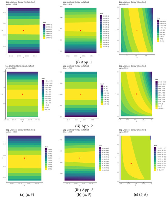
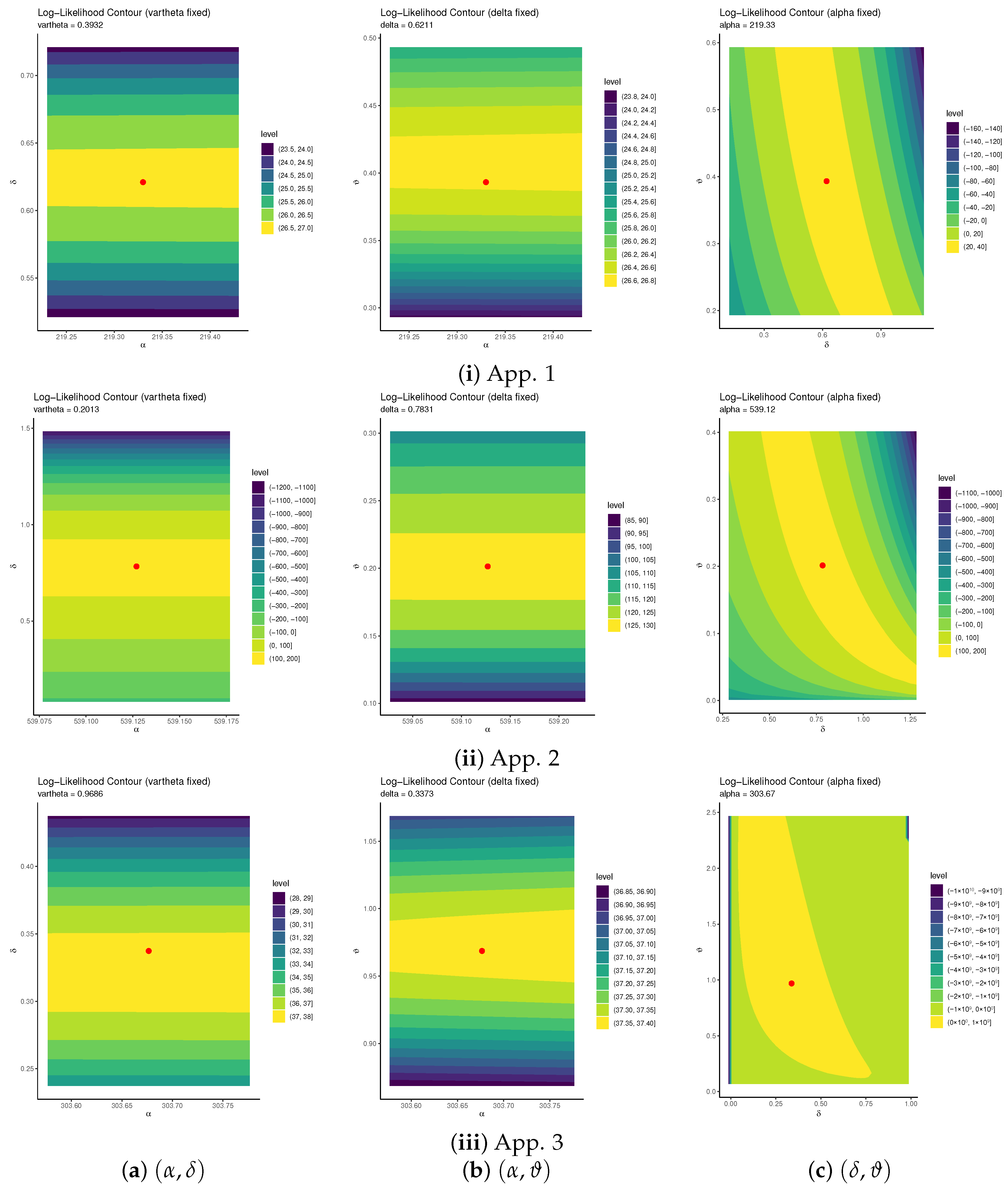
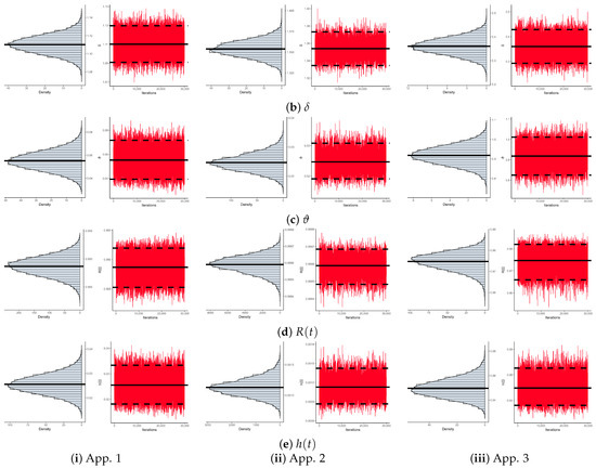
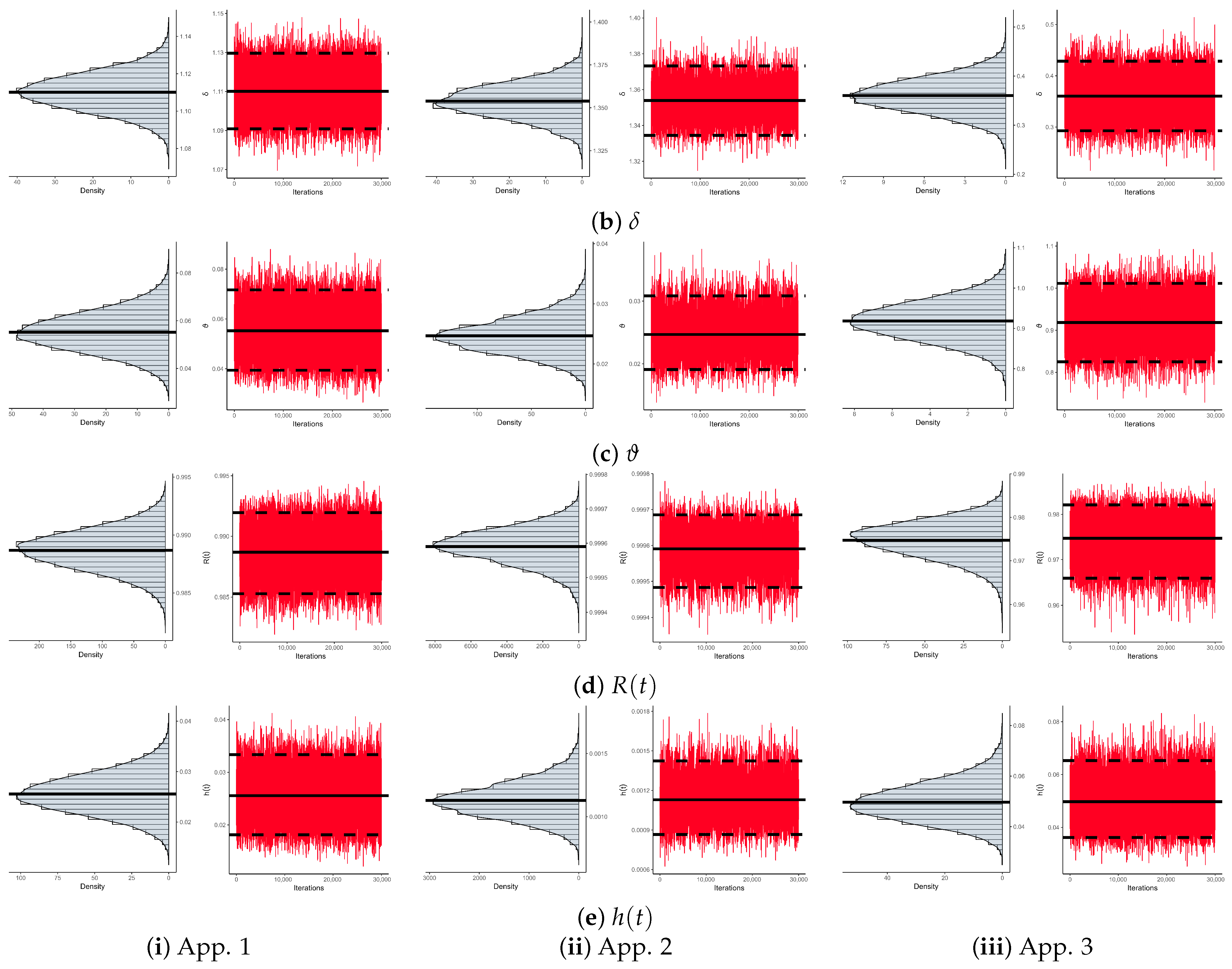
To illustrate the existence and uniqueness of the proposed MLEs for APW model parameters $\alpha$, $\delta$, and $\vartheta$, their log-likelihood contours were examined using $\mathcal{S}\left[A\right]$ as a representative sample from App. i (for $i=1,2,3$); see Figure 9. All contours of $\alpha$, $\delta$, and $\vartheta$ from the three datasets confirm that the estimates $\widehat{\alpha }$, $\widehat{\delta }$, and $\widehat{\vartheta }$ are existed and unique. The convergence behavior of the MCMC procedure was further validated using the remaining 30,000 iterations. Again, using $\mathcal{S}\left[A\right]$ as an example, Figure 10 presents the corresponding posterior density and trace plots for $\alpha$, $\delta$, $\vartheta$, $R\left(t\right)$, and $h\left(t\right)$. In each panel, the solid line represents the posterior mean (Bayesian point estimate), while the dashed lines denote the associated credible bounds. The plots exhibit satisfactory mixing and confirm that the adopted burn-in period is adequate. Furthermore, the Bayesian outputs display distinct yet approximately symmetric posterior distributions for $\alpha$, $\delta$, $\vartheta$, $R\left(t\right)$, and $h\left(t\right)$, indicating stable and well-behaved estimates. Furthermore, Table 8 presents key descriptive statistics for $\alpha$, $\delta$, $\vartheta$, $R\left(t\right)$, and $h\left(t\right)$, including the mean, mode, quartiles, standard deviation (SD), and skewness. These numerical summaries in Table 8 reinforce and validate the convergence behavior observed in the MCMC diagnostics shown in Figure 10, providing additional evidence of the stability and reliability of the posterior estimates.

Figure 9. The contour plots of $\alpha$, $\delta$, and $\vartheta$ from three sciences.

Figure 10. The MCMC plots of $\alpha$, $\delta$, $\vartheta$, $R\left(t\right)$, and $h\left(t\right)$ from three sciences.

Table 8. Statistical outcomes of $\alpha$, $\delta$, $\vartheta$, $R\left(t\right)$, and $h\left(t\right)$ from three sciences.

Data	Sample	Par.	Mean	Mode	Quartiles			SD	Skew.
					1st	2nd	3rd
App. 1	$\mathcal{S}\left[A\right]$	$\alpha$	4.33391	4.33467	4.32714	4.33393	4.34070	0.01000	−0.00903
		$\delta$	1.11015	1.07777	1.10338	1.11015	1.11689	0.00991	0.00967
		$\vartheta$	0.05520	0.05691	0.04962	0.05505	0.06068	0.00818	0.08969
		$R\left(t\right)$	0.98868	0.98807	0.98755	0.98872	0.98984	0.00169	−0.10023
		$h\left(t\right)$	0.02556	0.02618	0.02291	0.02547	0.02815	0.00387	0.10815
	$\mathcal{S}\left[B\right]$	$\alpha$	1.82643	1.80717	1.81967	1.82643	1.83319	0.01000	0.00200
		$\delta$	0.81614	0.80040	0.80940	0.81608	0.82290	0.00993	0.02455
		$\vartheta$	0.07966	0.07624	0.07333	0.07957	0.08597	0.00935	0.01373
		$R\left(t\right)$	0.96733	0.96419	0.96474	0.96736	0.96992	0.00382	−0.01231
		$h\left(t\right)$	0.05463	0.05209	0.05022	0.05456	0.05900	0.00650	0.02384
	$\mathcal{S}\left[C\right]$	$\alpha$	2.03528	2.02573	2.02852	2.03528	2.04204	0.01000	0.00224
		$\delta$	0.85176	0.84154	0.84501	0.85170	0.85851	0.00992	0.02365
		$\vartheta$	0.07541	0.08210	0.06927	0.07528	0.08147	0.00902	0.03321
		$R\left(t\right)$	0.97150	0.96869	0.96919	0.97154	0.97380	0.00340	−0.03523
		$h\left(t\right)$	0.04966	0.05401	0.04556	0.04958	0.05370	0.00603	0.04372
App. 2	$\mathcal{S}\left[A\right]$	$\alpha$	114.926	114.921	114.920	114.926	114.933	0.00997	0.00059
		$\delta$	1.35389	1.35572	1.34716	1.35383	1.36075	0.00991	−0.00235
		$\vartheta$	0.02468	0.02329	0.02261	0.02456	0.02655	0.00299	0.22745
		$R\left(t\right)$	0.99959	0.99961	0.99956	0.99959	0.99963	0.00005	−0.25602
		$h\left(t\right)$	0.00113	0.00106	0.00103	0.00112	0.00122	0.00014	0.25384
	$\mathcal{S}\left[B\right]$	$\alpha$	4.93630	4.95910	4.92948	4.93611	4.94280	0.01031	0.01007
		$\delta$	1.70453	1.70369	1.69793	1.70439	1.71070	0.00957	0.02356
		$\vartheta$	0.00261	0.00249	0.00225	0.00258	0.00293	0.00051	0.31229
		$R\left(t\right)$	0.99968	0.99969	0.99964	0.99968	0.99972	0.00006	−0.31943
		$h\left(t\right)$	0.00111	0.00105	0.00096	0.00110	0.00125	0.00022	0.31591
	$\mathcal{S}\left[C\right]$	$\alpha$	0.79646	0.79371	0.79516	0.79647	0.79783	0.00202	−0.01910
		$\delta$	1.73509	1.73186	1.73371	1.73505	1.73646	0.00199	0.00928
		$\vartheta$	0.00170	0.00158	0.00145	0.00168	0.00192	0.00036	0.51994
		$R\left(t\right)$	0.99943	0.99947	0.99936	0.99944	0.99951	0.00012	−0.52076
		$h\left(t\right)$	0.00199	0.00184	0.00169	0.00196	0.00224	0.00042	0.52032
App. 3	$\mathcal{S}\left[A\right]$	$\alpha$	1810.10	1810.08	1810.07	1810.10	1810.14	0.05005	−0.00588
		$\delta$	0.36025	0.34791	0.33688	0.36005	0.38397	0.03475	0.00642
		$\vartheta$	0.91851	0.96480	0.88636	0.91843	0.95079	0.04750	−0.01206
		$R\left(t\right)$	0.97472	0.97078	0.97206	0.97500	0.97762	0.00415	−0.38181
		$h\left(t\right)$	0.04971	0.05685	0.04443	0.04929	0.05462	0.00749	0.30133
	$\mathcal{S}\left[B\right]$	$\alpha$	10781.2	10781.1	10781.2	10781.2	10781.2	0.05000	0.00473
		$\delta$	0.27979	0.26787	0.25640	0.27948	0.30339	0.03493	0.02665
		$\vartheta$	1.12521	1.15590	1.09325	1.12481	1.15779	0.04807	0.00404
		$R\left(t\right)$	0.97440	0.97152	0.97153	0.97478	0.97765	0.00465	−0.47666
		$h\left(t\right)$	0.04954	0.05379	0.04436	0.04914	0.05433	0.00742	0.30446
	$\mathcal{S}\left[C\right]$	$\alpha$	10087.0	10086.9	10087.0	10087.0	10087.0	0.05004	0.00721
		$\delta$	0.30977	0.29764	0.28638	0.30941	0.33322	0.03478	0.04041
		$\vartheta$	1.25363	1.28428	1.22168	1.25322	1.28615	0.04797	0.00801
		$R\left(t\right)$	0.96473	0.96104	0.96105	0.96516	0.96883	0.00587	−0.42620
		$h\left(t\right)$	0.07607	0.08198	0.06913	0.07561	0.08260	0.01002	0.26379

7. Optimum Censoring

Selecting the most efficient sampling plan thus involves identifying the TII-PC plan that yields the maximum knowledge about the parameter(s) among all feasible alternatives, which is known as an optimum censoring design. In recent literature, determining the optimal censoring scheme has recently received considerable attention; see, for example, Pradhan and Kundu [30], Sen et al. [31], Mohammed et al. [32,33], and references therein. For fixed n and m, the possible censoring schemes correspond to all combinations of $(R_1,\dots ,R_m)$ satisfying $m+{\sum }_{i=1}^m{R}_i=n$. The first challenge, naturally, is to define appropriate measures of information based on a given progressive censoring plan, and the second is to develop a sound basis for comparing two different information measures corresponding to distinct censoring schemes; further details can be found in Nassar and Elshahhat [34].

The following discussion outlines several optimality criteria employed in this context. In practice, the goal is to determine the censoring scheme that conveys the greatest amount of information about the model parameters. Table 9 summarizes some widely used optimal censoring criteria (OCC) that can guide the selection of an efficient progressive censoring design. Under criterion $OCC\left[1\right]$, the aim is to maximize the FI trace, ${\mathbf{I}}_{3\times 3}(·)$. In contrast, for criteria $OCC\left[i\right],i=2,3$, the aim is to minimize the determinant and the trace of the AVC matrix, ${\mathbf{I}}_{3\times 3}^{-1}(·)$, respectively.

Table 9. Optimal censoring criteria.

Criterion	Method
$OCC\left[1\right]$	$\mathrm{Max}\mathrm{trace}\left({\mathbf{I}}_{3\times 3}(·)\right)$
$OCC\left[2\right]$	$\mathrm{Min}\mathrm{trace}\left({\mathbf{I}}_{3\times 3}^{-1}(·)\right)$
$OCC\left[3\right]$	$\mathrm{Min}\det \left({\mathbf{I}}_{3\times 3}^{-1}(·)\right)$
$OCC\left[4\right]$	$\mathrm{Min}\mathrm{var}\left(\log \left({\psi }_{\varrho }\right)\right),0<\varrho <1$

It is evident that criterion $OCC\left[4\right]$, which depends on the chosen value of $\varrho$, aims to minimize the variance of the logarithm of the MLE of the $\varrho$-th quantile. Consequently, for the APW distribution, the logarithmic form of $\log \left({\psi }_{\varrho }\right)$ is expressed as

$$\begin{array}{c}\hfill \log \left({\psi }_{\varrho }\right)={\left.{\left[-{\displaystyle \frac{1}{\vartheta }}\log \left[{\displaystyle \frac{\log \left(\frac{\alpha }{1+(\alpha -1)\varrho }\right)}{\log \left(\alpha \right)}}\right]\right]}^{{\displaystyle \frac{1}{\delta }}}\right|}_{(\alpha ,\delta ,\vartheta )=(\widehat{\alpha },\widehat{\delta },\widehat{\vartheta })},\end{array}$$

where $0<\varrho <1$. One may estimate the variance of $\log \left({\widehat{\psi }}_{\varrho }\right)$ using the delta approach. The ideal TII-PC design should be corresponds to the highest value of the criterion $OCC\left[1\right]$ and the smallest value of the criteria $OCC\left[i\right],i=2,3,4$.

We now illustrate the process of determining an OCC using the GTII-PHC samples $\mathcal{S}\left[i\right]$, $i=1,2,3$, generated from the proposed three real-world datasets. Table 10 presents the computed values of the optimality criteria $OCC\left[i\right]$ ($i=1,2,3,4$), based on the estimated parameters $\widehat{\alpha }$, $\widehat{\delta }$, and $\widehat{\vartheta }$ obtained from $\mathcal{S}\left[i\right]$ for each dataset.

Table 10. The optimum plans from three sciences.

Data	Sample$\downarrow \mathbf{OCC}\to$	[1]	[2]	[3]	[4]
$\mathbf{\varrho }\to$					0.3	0.6	0.9
App. 1	$\mathcal{S}\left[A\right]$	5109.911	89.8795	1.453 $\times {10}^{-3}$	9.77973	19.5065	90.9770
	$\mathcal{S}\left[B\right]$	1546.631	68.9891	3.036 $\times {10}^{-3}$	16.7309	118.598	2543.02
	$\mathcal{S}\left[C\right]$	2475.687	49.5805	1.146 $\times {10}^{-3}$	13.0701	64.2696	1033.74
App. 2	$\mathcal{S}\left[A\right]$	110,661.96	35.3734	1.524 $\times {10}^{-5}$	3.70311	6.96035	27.1487
	$\mathcal{S}\left[B\right]$	4,189,636.1	72.9964	2.138 $\times {10}^{-6}$	9.59617	27.1901	136.587
	$\mathcal{S}\left[C\right]$	7,912,514.2	4.00498	4.255 $\times {10}^{-8}$	13.9144	39.4256	198.050
App. 3	$\mathcal{S}\left[A\right]$	502.5953	140.827	1.288 $\times {10}^{-2}$	7.17616	63.2669	1460.43
	$\mathcal{S}\left[B\right]$	499.5968	70.4275	8.074 $\times {10}^{-3}$	13.4520	265.556	14,498.7
	$\mathcal{S}\left[C\right]$	518.5257	46.9813	4.589 $\times {10}^{-3}$	2.96774	37.1380	1428.31

The findings in Table 10 verify the efficiency of the proposed censoring strategies, aligning well with the performance trends developed in Section 5. Specifically:

• For App. 1:

  –

  For the criteria $OCC\left[i\right],i=1,3,4$, the left-censoring used in $\mathcal{S}\left[A\right]$ is the optimal than others;

  –

  For the criterion $OCC\left[2\right]$, the right-censoring used in $\mathcal{S}\left[C\right]$ is the optimal than others.

• For App. $i,i=2,3$:

  –

  For the criteria $OCC\left[4\right]$, the left-censoring used in $\mathcal{S}\left[A\right]$ is the optimal than others;

  –

  For the criterion $OCC\left[i\right],i=1,2,3$, the right-censoring used in $\mathcal{S}\left[C\right]$ is the optimal than others.

8. Concluding Remarks

This paper develops various inferential frameworks for analyzing censored lifetime data from the alpha–power Weibull model under generalized Type-II progressive hybrid censoring. The proposed censoring strategy extends traditional hybrid censoring structures by ensuring test termination within a fixed time while retaining the flexibility of progressive removals. Through rigorous likelihood formulation, likelihood estimators for the distributional parameters and related reliability measures are derived, and their asymptotic properties are examined using the observed Fisher information matrix. As closed-form solutions are infeasible, a Bayesian estimation procedure based on independent gamma priors is established. The Markov iterative algorithm is utilized to compute posterior estimates and credible intervals for both parameters and reliability functions, providing a practical alternative to classical inference. Comprehensive Monte Carlo simulations show that the proposed methods deliver accurate and stable estimates, with performance improving as the sample size increases or the censoring level decreases. Results indicate that Bayesian MCMC-based estimators, especially with informative priors, tend to outperform their frequentist counterparts in terms of bias, mean-square error, and coverage probability. Furthermore, the framework guarantees positive and theoretically sound interval limits for all parameters and reliability measures. Overall, this study advances the reliability literature by extending hybrid progressive censoring theory to a more general structure, formulating complete classical and Bayesian inferential procedures for the APW distribution, and validating their effectiveness via simulated and real data. The methodology enhances the flexibility and efficiency of reliability analysis under incomplete testing conditions and can be adapted to other generalized lifetime models or alternative censoring schemes in future research. Overall, this study successfully established an estimation framework for the APW distribution under GTII-PHC and verified the superiority of the Bayesian method through simulations and empirical applications.

References

- Bain, L.J.; Engelhardt, M. Statistical Analysis of Reliability and Life-Testing Models, 2nd ed.; Marcel Dekker: New York, NY, USA, 1991. [Google Scholar]
- Epstein, B. Truncated life tests in the exponential case. Ann. Math. Stat. 1954, 25, 555–564. [Google Scholar] [CrossRef] [Scilit]
- Childs, A.; Chandrasekar, B.; Balakrishnan, N.; Kundu, D. Exact likelihood inference based on Type-I and Type-II hybrid censored samples from the exponential distribution. Ann. Inst. Stat. Math. 2003, 55, 319–330. [Google Scholar] [CrossRef] [Scilit]
- Balakrishnan, N.; Cramer, E. The Art of Progressive Censoring; Springer: Birkhäuser, NY, USA, 2014. [Google Scholar]
- Ng, H.K.T.; Kundu, D.; Chan, P.S. Statistical analysis of exponential lifetimes under an adaptive Type-II progressive censoring scheme. Nav. Res. Logist. 2009, 56, 687–698. [Google Scholar] [CrossRef] [Scilit]
- Lee, K.; Sun, H.; Cho, Y. Exact likelihood inference of the exponential parameter under generalized Type II progressive hybrid censoring. J. Korean Stat. Soc. 2016, 45, 123–136. [Google Scholar] [CrossRef] [Scilit]
- Ateya, S.; Mohammed, H. Prediction under Burr-XII distribution based on generalized Type-II progressive hybrid censoring scheme. J. Egypt. Math. Soc. 2018, 26, 491–508. [Google Scholar]
- Nagy, M.; Bakr, M.E.; Alrasheedi, A.F. Analysis with Applications of the Generalized Type-II Progressive Hybrid Censoring Sample from Burr Type-XII Model. Math. Probl. Eng. 2022, 2022, 1241303. [Google Scholar] [CrossRef] [Scilit]
- Cho, S.; Lee, K. Exact likelihood inference for a competing risks model with generalized type II progressive hybrid censored exponential data. Symmetry 2021, 13, 887. [Google Scholar] [CrossRef] [Scilit]
- Wang, L.; Zhou, Y.; Lio, Y.; Tripathi, Y.M. Inference for Kumaraswamy distribution under generalized progressive hybrid censoring. Symmetry 2022, 14, 403. [Google Scholar] [CrossRef] [Scilit]
- Alqasem, O.A.; Abd Elwahab, M.E.; Abo-Kasem, O.E.; Elshahhat, A. Evaluation of new Garima data using type-II generalized progressive-hybrid technique and its application to a sodium–sulfur battery. AIP Adv. 2024, 14, 105002. [Google Scholar] [CrossRef] [Scilit]
- Mohammed, H.S.; Abo-Kasem, O.E.; Elshahhat, A. Computational analysis of generalized progressive hybrid log-logistic model and its modeling for physics and engineering applications. AIMS Math. 2025, 10, 10709–10739. [Google Scholar] [CrossRef] [Scilit]
- Nassar, M.; Alzaatreh, A.; Mead, M.; Abo-Kasem, O. Alpha power Weibull distribution: Properties and applications. Commun. Stat.-Theory Methods 2017, 46, 10236–10252. [Google Scholar] [CrossRef] [Scilit]
- Mahdavi, A.; Kundu, D. A new method for generating distributions with an application to exponential distribution. Commun. Stat.-Theory Methods 2017, 46, 6543–6557. [Google Scholar] [CrossRef] [Scilit]
- Peng, K.; Chen, W. Maximum likelihood estimators and properties of the parameters of the Power Ailamujia distribution under ranked set sampling. J. Stat. Comput. Simul. 2025, 95, 3705–3727. [Google Scholar] [CrossRef] [Scilit]
- Gelman, A.; Carlin, J.B.; Stern, H.S.; Rubin, D.B. Bayesian Data Analysis, 2nd ed.; Chapman and Hall/CRC: New York, NY, USA, 2004. [Google Scholar]
- Lawless, J.F. Statistical Models and Methods for Lifetime Data; John Wiley and Sons: New York, NY, USA, 2011. [Google Scholar]
- Greene, W.H. Econometric Analysis, 4th ed.; Prentice-Hall: New York, NY, USA, 2000. [Google Scholar]
- Meeker, W.Q.; Escobar, L.A. Statistical Methods for Reliability Data; John Wiley & Sons: Hoboken, NJ, USA, 2014. [Google Scholar]
- Henningsen, A.; Toomet, O. maxLik: A package for maximum likelihood estimation in R. Comput. Stat. 2011, 26, 443–458. [Google Scholar] [CrossRef] [Scilit]
- Plummer, M.; Best, N.; Cowles, K.; Vines, K. CODA: Convergence diagnosis and output analysis for MCMC. R News 2006, 6, 7–11. [Google Scholar]
- Kundu, D. Bayesian inference and life testing plan for the Weibull distribution in presence of progressive censoring. Technometrics 2008, 50, 144–154. [Google Scholar] [CrossRef] [Scilit]
- Elshahhat, A.; Abu El Azm, W.S. Statistical reliability analysis of electronic devices using generalized progressively hybrid censoring plan. Qual. Reliab. Eng. Int. 2022, 38, 1112–1130. [Google Scholar] [CrossRef] [Scilit]
- Hawkins, D.M. Diagnostics for conformity of paired quantitative measurements. Stat. Med. 2002, 21, 1913–1935. [Google Scholar] [CrossRef] [Scilit]
- Elshahhat, A.; Alotaibi, R.; Nassar, M. Statistical inference of the Birnbaum-Saunders model using adaptive progressively hybrid censored data and its applications. AIMS Math. 2024, 9, 11092–11121. [Google Scholar] [CrossRef] [Scilit]
- Maurya, S.K.; Goyal, T. A New Decreasing Failure Rate Distribution and Its Real Life Application. Int. J. Stat. Reliab. Eng. 2023, 10. Available online: https://ijsreg.com/article/view/a-new-decreasing-failure-rate-distribution-and-its-real-life-application (accessed on 1 October 2025).
- Mudholkar, G.S.; Srivastava, D.K. Exponentiated Weibull family for analyzing bathtub failure-rate data. IEEE Trans. Reliab. 1993, 42, 299–302. [Google Scholar] [CrossRef] [Scilit]
- Oguntunde, P.E.; Balogun, O.S.; Okagbue, H.I.; Bishop, S.A. The Weibull-exponential distribution: Its properties and applications. J. Appl. Sci. 2015, 15, 1305–1311. [Google Scholar] [CrossRef] [Scilit]
- Weibull, W. A statistical distribution function of wide applicability. J. Appl. Mech. 1951, 18, 93–297. [Google Scholar] [CrossRef] [Scilit]
- Pradhan, B.; Kundu, D. Inference and optimal censoring schemes for progressively censored Birnbaum–Saunders distribution. J. Stat. Plan. Inference 2013, 143, 1098–1108. [Google Scholar] [CrossRef] [Scilit]
- Sen, T.; Tripathi, Y.M.; Bhattacharya, R. Statistical inference and optimum life testing plans under Type-II hybrid censoring scheme. Ann. Data Sci. 2018, 5, 679–708. [Google Scholar] [CrossRef] [Scilit]
- Mohammed, H.S.; Abo-Kasem, O.E.; Elshahhat, A. Analysis and optimum removals of unit-Weibull data from progressive first-failure censoring and its modeling in chemistry and physics. J. Stat. Comput. Simul. 2025, 95, 3970–4002. [Google Scholar] [CrossRef] [Scilit]
- Mohammed, H.S.; Abo-Kasem, O.E.; Elshahhat, A. Optimum Progressive Data Analysis and Bayesian Inference for Unified Progressive Hybrid INH Censoring with Applications to Diamonds and Gold. Axioms 2025, 14, 559. [Google Scholar] [CrossRef] [Scilit]
- Nassar, M.; Elshahhat, A. Estimation procedures and optimal censoring schemes for an improved adaptive progressively Type-II censored Weibull distribution. J. Appl. Stat. 2024, 51, 1664–1688. [Google Scholar] [CrossRef] [Scilit] [PubMed]
Disclaimer/Publisher’s Note: The statements, opinions and data contained in all publications are solely those of the individual author(s) and contributor(s) and not of MDPI and/or the editor(s). MDPI and/or the editor(s) disclaim responsibility for any injury to people or property resulting from any ideas, methods, instructions or products referred to in the content. |
© 2025 by the authors. Licensee MDPI, Basel, Switzerland. This article is an open access article distributed under the terms and conditions of the Creative Commons Attribution (CC BY) license (https://creativecommons.org/licenses/by/4.0/).