Semi-Analytical Solutions for the Qi-Type Dynamical System

Abstract

The aim of present paper is to obtain approximate semi-analytical solutions for the Qi-type dynamical system, while neglecting its chaotic behaviors. These solutions are derived using the Optimal Auxiliary Functions Method (OAFM). The impact of the system’s physical parameters is also investigated. A special case, involving a constant of motion, is considered for which closed-form solutions are obtained. The dynamical system is reduced to a second-order nonlinear differential equation, which is analytically solved through the OAFM procedure. The influence of initial conditions on the system is explored, specifically regarding the presence or absence of symmetries. An exact parametric solution is obtained for a particular case. A good agreement between the analytical and corresponding numerical results is demonstrated, highlighting the accuracy of the proposed method. A comparative analysis underlines the advantages of the OAFM compared to other analytical methods. These findings have numerous technological applications, such as in nonlinear circuits with three channels that involve adapted physical parameters to ensure effective functioning of electronic circuits, as well as in information storage, encryption, and communication systems.

1. Introduction

Mankind, by its very nature, has constantly sought to explain the complex phenomena that govern the environment and society, leading to the development of fundamental sciences such as mathematics, physics, and biology. Many natural phenomena in fields like meteorology, engineering, chemistry, physics, aerodynamics [1], economics, biology, and medicine can be partially modeled through various nonlinear dynamical systems.

With advances in computer science, the interest in protecting and securing information transmission has grown. Today, achieving enhanced encryption is a pressing issue. Modern encryption relies on algorithms involving non-linear systems and dynamic combinations of such systems, utilizing increasingly inventive mathematical models.

The surrounding reality can often be understood as the interaction of complex nonlinear dynamical systems. It has been shown that even very simple nonlinear systems can exhibit highly complex, seemingly random behavior. Chaos theory attempts to explain and predict this apparently unpredictable behavior of nonlinear systems, even in the short term.

Although ideas related to chaos theory have existed for a long time, they were first crystallized by Lorenz, who created a three-dimensional mathematical model of atmospheric circulation—a deterministic system with unpredictable behavior.

Chaos is characterized by a high sensitivity of associated nonlinear systems to changes in initial conditions. In 1963, Lorenz [2] proposed the first mathematical system to investigate chaos through nonlinear equations. This marked the starting point for the development of complexity science and the exploration of chaos generation for engineering applications. Li and Yorke, in 1975, defined the concept of chaos in dynamical system [3]. In 1976, Rössler proposed a system of three nonlinear ordinary differential equations with an algebraic form simpler than Lorenz’z model [4], and later offered a further simplified model in 1979 [5]. In 1986, Matsumoto et al. developed an autonomous chaotic system based on the “Chua circuit” [6]. In 1999, Chen and Ueta proposed a new chaotic system, now known as the Chen system [7]. Lü et al. [8] subsequently developed another system, representing a transition between the Lorenz and Chen systems. A unified chaotic system between the Lorenz and the Chen systems was investigated by Lü et al. [9]. Sprott introduced generic three-dimensional systems with quadratic nonlinearities, identifying 19 different chaotic systems with no obvious transformations between them [10,11,12]. Van Gorder and Roy Choudhury proposed a new three-dimensional system with quadratic nonlinearity [13]. Among the three-dimensional chaotic systems, some of the most well-known are [14]: the Chen system, the Lü system, the Qi system, the Chua system, the Sprott system, and the Jerk system, among others. Qi and Liang [15] introduced a nonlinear three-dimensional chaotic system that is distinct from the Alligood, Rössler, Chen, and Lorenz systems. In their system, Qi incorporated a nonlinear term into each equation to enhance the system’s complexity and unpredictability. Based on the chaotic system proposed by Qi, new four-dimensional hyperchaotic systems have been developed. Potential technological applications of these systems include circuit design for telecommunications, biomedical engineering, and information storage. Prior research into the dynamic behaviors of the Qi system—including aspects such as dissipativity, equilibrium and stability, existence of attractors, periodic and quasi-periodic behaviors, and bifurcation analysis—can be found in [16].

A hyperchaotic system benefits from multiple chaotic behaviors acting simultaneously. Compared to regular chaotic systems, hyperchaotic systems display more complex dynamics, with multiple positive Lyapunov exponents indicating a higher degree of unpredictability and complexity [17]. Since their introduction by Rössler, hyperchaotic systems have seen steady progress in research and applications.

In recent years, with the widespread application of chaos theory, extensive research has been conducted, leading to numerous new findings. The Lyapunov exponent is a measure of the rate at which trajectories of a dynamical system converge or diverge. Nonlinear three-dimensional chaotic systems are characterized by a single positive Lyapunov exponent. For a hyperchaotic (continuous) system, the minimum dimensionality is four. A four-dimensional autonomous system is considered hyperchaotic if it has two positive, one zero, and one negative Lyapunov exponent. In contrast, a 4D system is classified as chaotic if it has one positive, one zero, and two negative Lyapunov exponents. If the system has two zero and two negative Lyapunov exponents, it is quasi-periodic. A 4D system is periodic if it has one Lyapunov exponent equal to zero and the other three are negative. Recently, Zghair et al. proposed a suitable seven-dimensional hyperchaotic system with control mechanisms [18].

Parabolic PDE–ODE systems with input saturation have been analyzed by [19]. Other PDE systems incorporating distributed delays are described by [20].

As the number of dimensions in a chaotic system increases, analyzing its behaviors becomes increasingly challenging. Despite these challenges, higher dimensional chaotic systems are often encountered in biological networks, electronics, circuits, secure communications, and image processing. These systems have more complex structures, involve more variables and parameters, and are particularly suitable for applications requiring complexity, such as network security and data encryption.

Our paper provides approximate semi-analytical solutions for the Qi-type dynamical system using OAFM, specifically focusing on the existence or non-existence of symmetries.

The structure of this paper is as follows: Section 1 introduces the topic, while Section 2 presents the Qi-type dynamical system, including a prime integral (constant of motion) and its closed-form solutions. An exact parametric solution is also discussed in this section. Section 3 describes the Optimal Auxiliary Functions Method (OAFM) and its application in deriving semi-analytical solutions. Section 4 includes numerical results and highlights the advantages of the applied method. Finally, the concluding remarks are presented in Section 5.

2. Preliminaries

2.1. The Qi Dynamical System

The Qi dynamical system is written as [16]

$$\left\{\begin{array}{c}\dot{x}=a(y-x)+yz\hfill \\ \dot{y}=cx-y-xz\hfill \\ \dot{z}=xy-bz\hfill \end{array}\right.,a,b,c\in {\mathbb{R}}_{+}.$$

(1)

The initial conditions are:

$$x\left(0\right)=x_0,y\left(0\right)=y_0,z\left(0\right)=z_0.$$

(2)

2.2. Closed-Form Solutions

The following cases are investigated in this paper.

2.2.1. $a=b=0$, $c>0$ with $x_0^2-z_0^2\ne 0$

In this case, the system (1) becomes

$$\left\{\begin{array}{c}\dot{x}=yz\hfill \\ \dot{y}=cx-y-xz\hfill \\ \dot{z}=xy\hfill \end{array}\right.,c\in {\mathbb{R}}_{+}.$$

(3)

The system given by Equation (3) admits a unique constant of motion satisfying the initial conditions given by Equation (2), namely

$$H(x,y,z)={\displaystyle \frac{1}{2}}{x}^2-{\displaystyle \frac{1}{2}}{z}^2={\displaystyle \frac{1}{2}}{x}_0^2-{\displaystyle \frac{1}{2}}{z}_0^2.$$

(4)

Remark 1.

It is easy to see that the system (3) admits the symmetry with respect to the $Oz$-axis, because it is invariant under the transformation $(x,y,z)\to (-x,-y,z)$.

The initial conditions $x_0$ and $z_0$ can influence the closed-form solutions of the system (3).

For $x_0>z_0>0$, $R=\sqrt{x_0^2-z_0^2}$, the transformation

$$\left\{\begin{array}{c}x=R{\displaystyle \frac{1+u^2}{1-u^2}}\hfill \\ y={\displaystyle \frac{2\dot{u}}{1-u^2}}\hfill \\ z=R{\displaystyle \frac{2u}{1-u^2}}\hfill \end{array}\right.,$$

(5)

leads to closed-form solutions of the system (3), where the unknown smooth function $u\left(t\right)$ is solution of the following problem:

$$\left\{\begin{array}{c}2\ddot{u}(1-u^2)+4u{\left(\dot{u}\right)}^2-cR(1-u^4)+2\dot{u}(1-u^2)+2R^{2}u(1+u^2)=0\hfill \\ u\left(0\right)={\displaystyle \frac{|z_0|}{|R+x_0|}},\dot{u}\left(0\right)={\displaystyle \frac{1}{2}}{y}_0(1-u^2\left(0\right))\hfill \end{array}\right.,c\in {\mathbb{R}}_{+}.$$

(6)

In the next section, semi-analytical solutions to the nonlinear problem (6) via OAFM procedure are presented.

Remark 2.

(a) If $x_0>0$, $z_0<0$, $x_0^2-z_0^2>0$, $R=\sqrt{x_0^2-z_0^2}$, then by transformation

$$\left\{\begin{array}{c}x=R{\displaystyle \frac{1+u^2}{1-u^2}}\hfill \\ y={\displaystyle \frac{2\dot{u}}{1-u^2}}\hfill \\ z=-R{\displaystyle \frac{2u}{1-u^2}}\hfill \end{array}\right.,$$

(7)

the closed-form solutions of the system (3) can be obtained. Here, the unknown function $u\left(t\right)$ is solution of the nonlinear problem:

$$\left\{\begin{array}{c}2\ddot{u}(1-u^2)+4u{\left(\dot{u}\right)}^2-cR(1-u^4)+2\dot{u}(1-u^2)-2R^{2}u(1+u^2)=0\hfill \\ u\left(0\right)={\displaystyle \frac{|z_0|}{|R+x_0|}},\dot{u}\left(0\right)={\displaystyle \frac{1}{2}}{y}_0(1-u^2\left(0\right))\hfill \end{array}\right.,c\in {\mathbb{R}}_{+}.$$

(8)

(b) If $x_0<0$, $z_0>0$, $x_0^2-z_0^2>0$, $R=\sqrt{x_0^2-z_0^2}$, then by transformation

$$\left\{\begin{array}{c}x=-R{\displaystyle \frac{1+u^2}{1-u^2}}\hfill \\ y={\displaystyle \frac{2\dot{u}}{1-u^2}}\hfill \\ z=+R{\displaystyle \frac{2u}{1-u^2}}\hfill \end{array}\right.,$$

(9)

the closed-form solutions of the system (3) can be obtained. Here, the unknown function $u\left(t\right)$ is solution of the nonlinear problem:

$$\left\{\begin{array}{c}2\ddot{u}(1-u^2)+4u{\left(\dot{u}\right)}^2+cR(1-u^4)+2\dot{u}(1-u^2)-2R^{2}u(1+u^2)=0\hfill \\ u\left(0\right)={\displaystyle \frac{|z_0|}{|R+x_0|}},\dot{u}\left(0\right)={\displaystyle \frac{1}{2}}{y}_0(1-u^2\left(0\right))\hfill \end{array}\right.,c\in {\mathbb{R}}_{+}.$$

(10)

(c) If $x_0<0$, $z_0<0$, $x_0^2-z_0^2>0$, $R=\sqrt{x_0^2-z_0^2}$, then by transformation

$$\left\{\begin{array}{c}x=-R{\displaystyle \frac{1+u^2}{1-u^2}}\hfill \\ y={\displaystyle \frac{2\dot{u}}{1-u^2}}\hfill \\ z=-R{\displaystyle \frac{2u}{1-u^2}}\hfill \end{array}\right.,$$

(11)

the closed-form solutions of the system (3) can be obtained. Here, the unknown function $u\left(t\right)$ is solution of the nonlinear problem:

$$\left\{\begin{array}{c}2\ddot{u}(1-u^2)+4u{\left(\dot{u}\right)}^2+cR(1-u^4)+2\dot{u}(1-u^2)-2R^{2}u(1+u^2)=0\hfill \\ u\left(0\right)={\displaystyle \frac{|z_0|}{|R+x_0|}},\dot{u}\left(0\right)={\displaystyle \frac{1}{2}}{y}_0(1-u^2\left(0\right))\hfill \end{array}\right.,c\in {\mathbb{R}}_{+}.$$

(12)

(d) In all situations when $z_0^2-x_0^2>0$, the closed-form solutions can be obtained by changing between them the functions $x\left(t\right)$ and $z\left(t\right)$ in all Equations (5), (7), (9), (11), respectively. The constant R well be $R=\sqrt{z_0^2-x_0^2}$.

2.2.2. Exact Parametric Solution for $a=b=0$, $c>0$ with $x_0^2-z_0^2=0$

In this case $|x_0|=|z_0|$. The constant of motion given by Equation (4) leads to $\left|x\right(t\left)\right|=\left|z\right(t\left)\right|$, namely:

(a) if $x_0=z_0>0$ (or $x_0=z_0<0$) then $x\left(t\right)=z\left(t\right)$; the system (3) becomes

$$\left\{\begin{array}{c}\dot{x}=xy\hfill \\ \dot{y}=cx-y-x^2\hfill \\ z=x\hfill \end{array}\right.,c\in {\mathbb{R}}_{+}.$$

(13)

Remark 3.

The system (13) does not admit symmetries.

This system is equivalent with the following equation

$$\begin{array}{c}\ddot{x}x-{\left(\dot{x}\right)}^2-c{x}^3+x\dot{x}+x^4=0\hfill \end{array},c\in {\mathbb{R}}_{+},$$

(14)

with $x\left(0\right)=x_0>0$ (or $x\left(0\right)=x_0<0$).

In the next section, the semi-analytical solutions of the Equation (14), denoted by $\overline{x}\left(t\right)$ or ${\overline{x}}_{OAFM}\left(t\right)$, are obtained.

In this case, the exact parametric solution of the second equation from Equation (13) can be obtained via the change of variable given by $y\left(t\right)=Y\left(x\right(t\left)\right)$. The derivative $\dot{y}$ becomes $\dot{y}={\displaystyle \frac{dy}{dt}}={\displaystyle \frac{dY}{dx}}{\displaystyle \frac{dx}{dt}}=\dot{x}{\displaystyle \frac{dY}{dx}}=xy{\displaystyle \frac{dY}{dx}}=xY{\displaystyle \frac{dY}{dx}}$. Now, the second equation from Equation (13) becomes:

$$\begin{array}{c}Y{\displaystyle \frac{dY}{dx}}=c-{\displaystyle \frac{Y}{x}}-x\hfill \end{array},c\in {\mathbb{R}}_{+},$$

(15)

with $Y\left(x\left(0\right)\right)=Y\left(x_0\right)=y\left(0\right)=y_0$.

Assuming that the condition $\left|{\displaystyle \frac{c-x}{c}}\right|<1$ is true, the function ${\displaystyle \frac{1}{x}}$ can be expanding in power series as

$$\begin{array}{c}{\displaystyle \frac{1}{x}=\frac{1}{c}\sum _{n=0}^{\infty }{\left(\frac{c-x}{c}\right)}^n}\hfill \end{array},c\in {\mathbb{R}}_{+}.$$

(16)

In this way, it is more convenient to consider the following power series for the function $Y\left(x\right)$:

$$\begin{array}{c}{\displaystyle Y\left(x\right)=C_0+\sum _{n=1}^{\infty }\frac{C_n}{n}{\left(\frac{c-x}{c}\right)}^n}\hfill \end{array},c\in {\mathbb{R}}_{+}.$$

(17)

Using Equation (17) the initial condition $Y\left(x_0\right)=y_0$ yields:

$$\begin{array}{c}{\displaystyle C_0=y_0-\sum _{n=1}^{\infty }\frac{C_n}{n}{\left(\frac{c-x_0}{c}\right)}^n}\hfill \end{array},c\in {\mathbb{R}}_{+},x_0\ne c.$$

(18)

Substituting Equations (16) and (17) into Equation (15) the following identity holds:

$$\begin{array}{c}{\displaystyle \left[C_0+\frac{C_1}{1c}(c-x)+\frac{C_2}{2c^2}{(c-x)}^2+\frac{C_3}{3c^3}{(c-x)}^3+\dots \right]\times }\hfill \\ \left[{\displaystyle \frac{1}{c^1}}(1-C_1)+{\displaystyle \frac{1}{c^2}}(1-C_2)(c-x)+{\displaystyle \frac{1}{c^3}}(1-C_3){(c-x)}^2+{\displaystyle \frac{1}{c^4}}(1-C_4){(c-x)}^3+\dots \right]=c-x.\hfill \end{array}$$

(19)

Identifying the same powers of $c-x$, the following nonlinear recurrence relations hold:

$$\left\{\begin{array}{c}{\displaystyle C_0(1-C_1)=0}\hfill \\ {\displaystyle C_0(1-C_2)+C_1(1-C_1)=c^2}\hfill \\ {\displaystyle C_0(1-C_3)+\frac{C_1}{1}(1-C_2)+\frac{C_2}{2}(1-C_1)=0}\hfill \\ {\displaystyle C_0(1-C_4)+\frac{C_1}{1}(1-C_3)+\frac{C_2}{2}(1-C_2)+\frac{C_3}{3}(1-C_1)=0}\hfill \\ \dots \dots \dots \dots \hfill \\ {\displaystyle C_0(1-C_k)+\frac{C_1}{1}(1-C_{k-1})+\frac{C_2}{2}(1-C_{k-2})+\frac{C_3}{3}(1-C_{k-3})+\dots }\hfill \\ {\displaystyle +\frac{C_{k-3}}{k-3}(1-C_3)+\frac{C_{k-2}}{k-2}(1-C_2)+\frac{C_{k-1}}{k-1}(1-C_1)=0}\hfill \\ {\displaystyle C_0(1-C_{k+1})+\frac{C_1}{1}(1-C_k)+\frac{C_2}{2}(1-C_{k-1})+\frac{C_3}{3}(1-C_{k-2})+\dots }\hfill \\ {\displaystyle +\frac{C_{k-3}}{k-3}(1-C_4)+\frac{C_{k-2}}{k-2}(1-C_3)+\frac{C_{k-1}}{k-1}(1-C_2)+\frac{C_k}{k}(1-C_1)=0}\hfill \\ \dots \dots \dots \dots \hfill \end{array}\right..$$

(20)

Obviously $C_0\ne 0$, else from ${\displaystyle C_0(1-C_2)+C_1(1-C_1)=1}$ the therm $C_1$ is not a real number.

From the relations given by Equation (20), the following nonlinear recurrence relations hold:

$$\begin{array}{c}{\displaystyle C_0(C_{k+1}-C_k)+\frac{C_1}{1}(C_k-C_{k-1})+\frac{C_2}{2}(C_{k-1}-C_{k-2})+\frac{C_3}{3}(C_{k-2}-C_{k-3})+\dots }\hfill \\ {\displaystyle +\frac{C_{k-3}}{k-3}(C_4-C_3)+\frac{C_{k-2}}{k-2}(C_3-C_2)+\frac{C_{k-1}}{k-1}(C_2-C_1)+\frac{C_k}{k}(C_1-1)=0,k\ge 3}\hfill \end{array},c\in {\mathbb{R}}_{+}.$$

(21)

The finding of the real sequence ${\left(C_k\right)}_{k\ge 1}$ and the limit ${\displaystyle \underset{n\to \infty }{lim}\sqrt[n]{|C_n|}}$, respectively, remains an open problem.

Assuming the existence of the limit ${\displaystyle \underset{n\to \infty }{lim}\sqrt[n]{|C_n|}=\tilde{C}\in \mathbb{R}}$, the power series from Equation (17) is absolute convergent (via Abel’s Theorem from Mathematical Analysis) on the interval $(-R_{max},R_{max})$, where $R_{max}={\displaystyle \frac{1}{{\displaystyle \underset{n\to \infty }{lim}\sqrt[n]{\left|\frac{C_n}{n}{\left(\frac{c-x}{c}\right)}^n\right|}}}}=|{\displaystyle \frac{1}{\tilde{C}}}{\displaystyle \frac{c}{c-x}}|$ and uniform convergent on each interval $[-r,r]\subset (-R_{max},R_{max})$.

The following Theorem assures us that the series form Equation (16) is well-defined.

Theorem 1.

The sequence $\left(C_n\right)$ defined by Equation (21) is convergent if and only if the series ${\displaystyle \sum _{k=1}^{\infty }\frac{|C_k|}{k}}$ is convergent.

Proof. 

“⇒”

Assume that the sequence $\left(C_n\right)$ defined by Equation (21) is convergent. Let be ${\displaystyle L=\underset{n\to \infty }{lim}{C}_n}$ finite. Then

$$(\forall )\epsilon >0,(\exists )n_0=n_0\left(\epsilon \right)\in \mathbb{N},(\forall )n\ge n_0\Rightarrow |C_n-L|<\epsilon .$$

Using the Cauchy’s criteria from Mathematical Analysis it is more convenient to show that the series ${\displaystyle \sum _{k=1}^{\infty }\frac{|C_{2^k}|}{2^k}}$ is convergent.

Let $p\ge 1$ be an arbitrary fixed number and denote by ${\displaystyle s_n=\sum _{k=1}^n\frac{|C_{2^k}|}{2^k}}$. Then the following relations hold:

$$|s_{n+p}-s_n|=|{\displaystyle \frac{C_{2^{n+1}}}{2^{n+1}}}+{\displaystyle \frac{C_{2^{n+2}}}{2^{n+2}}}+\dots +{\displaystyle \frac{C_{2^{n+p}}}{2^{n+p}}}|$$

$$\le {\displaystyle \frac{L+\epsilon }{2^{n+1}}}+{\displaystyle \frac{L+\epsilon }{2^{n+2}}}+\dots +{\displaystyle \frac{L+\epsilon }{2^{n+p}}}={\displaystyle \frac{L+\epsilon }{2^n}}\left({\displaystyle \frac{1}{2}}+{\displaystyle \frac{1}{2^2}}+\dots +{\displaystyle \frac{1}{2^p}}\right)$$

$$={\displaystyle \frac{L+\epsilon }{2^n}}\left(1-{\displaystyle \frac{1}{2^p}}\right)<{\displaystyle \frac{L+\epsilon }{2^n}}.$$

However, the sequence ${\displaystyle \frac{L+\epsilon }{2^n}}$ is convergent toward 0. Therefore, the sequence $\left(s_n\right)$ is a Cauchy sequence, so it is convergent. Hence, the series ${\displaystyle \sum _{k=1}^{\infty }\frac{|C_{2^k}|}{2^k}}$ is convergent. Thus, the series ${\displaystyle \sum _{k=1}^{\infty }\frac{|C_k|}{k}}$ is convergent.

“⇐”

Assume that the series ${\displaystyle \sum _{k=1}^{\infty }\frac{|C_k|}{k}}$ is convergent. Then the series ${\displaystyle \sum _{k=1}^{\infty }\frac{C_k}{k}{\left(\frac{c-x_0}{c}\right)}^k}$ is convergent, so $C_0$ defined in Equation (18) is a finite number because

$${\displaystyle \left|\sum _{k=1}^{\infty }\frac{C_k}{k}{\left(\frac{c-x_0}{c}\right)}^k\right|\le \sum _{k=1}^{\infty }\frac{\left|C_k\right|}{k}\left|{\left(\frac{c-x_0}{c}\right)}^k\right|<\sum _{k=1}^{\infty }\frac{\left|C_k\right|}{k}<\infty .}$$

It is more convenient to show that the sequence $\left(C_n\right)$ is a Cauchy sequence.

From Equations (20) and (21) the following relations hold:

$$\begin{array}{c}|C_2-C_1|={\displaystyle \frac{c^2}{\left|C_0\right|}}\hfill \\ |C_3-C_2|=|{\displaystyle \frac{c^2}{C_0}}-{\displaystyle \frac{C_1}{1}}(C_2-C_1)|\le {\displaystyle \frac{c^2}{\left|C_0\right|}}+{\displaystyle \frac{c^2}{\left|C_0\right|}}={\displaystyle \frac{2c^2}{\left|C_0\right|}}\hfill \\ \left|C_0\right||C_4-C_3|\le \left|{\displaystyle \frac{C_1}{1}}\right||C_3-C_2|+{\displaystyle \frac{1}{2}}\left|C_2\right||C_2-C_1|\le {\displaystyle \frac{2c^2}{\left|C_0\right|}}+{\displaystyle \frac{1}{2}}{\displaystyle \frac{c^2}{\left|C_0\right|}}\left|C_2\right|\hfill \\ \Rightarrow |C_4-C_3|\le {\displaystyle \frac{c^2}{|C_0{|}^2}}\left(2+{\displaystyle \frac{1}{2}}\left|C_2\right|\right)\hfill \\ \dots \dots \dots \dots \dots \hfill \\ |C_{n+1}-C_n|\le {\displaystyle \frac{c^2}{|C_0{|}^{n-1}}}\left(2+{\displaystyle \frac{1}{2}}\left|C_2\right|+{\displaystyle \frac{1}{3}}\left|C_3\right|+\dots +{\displaystyle \frac{1}{n-1}}\left|C_{n-1}\right|\right)\hfill \\ ={\displaystyle \frac{c^2}{|C_0{|}^{n-1}}}\left({\displaystyle 1+\sum _{k=1}^{n-1}\frac{\left|C_k\right|}{k}}\right),n\ge 3\hfill \end{array}$$

Let be $p\ge 1$ a fixed number. Then, the following inequality holds

$$\begin{array}{c}|C_{n+p}-C_n|\hfill \\ =|C_{n+p}-C_{n+p-1}+C_{n+p-1}-C_{n+p-2}+\dots +C_{n+2}-C_{n+1}+C_{n+1}-C_n|\hfill \\ \le |C_{n+p}-C_{n+p-1}|+|C_{n+p-1}-C_{n+p-2}|+\dots +|C_{n+2}-C_{n+1}|+|C_{n+1}-C_n|\hfill \\ \le {\displaystyle \frac{c^2}{|C_0{|}^{n+p-2}}}\left({\displaystyle 1+\sum _{k=1}^{n+p-2}\frac{\left|C_k\right|}{k}}\right)+{\displaystyle \frac{c^2}{|C_0{|}^{n+p-3}}}\left({\displaystyle 1+\sum _{k=1}^{n+p-3}\frac{\left|C_k\right|}{k}}\right)+\dots \hfill \\ +{\displaystyle \frac{c^2}{|C_0{|}^n}}\left({\displaystyle 1+\sum _{k=1}^n\frac{\left|C_k\right|}{k}}\right)+{\displaystyle \frac{c^2}{|C_0{|}^{n-1}}}\left({\displaystyle 1+\sum _{k=1}^{n-1}\frac{\left|C_k\right|}{k}}\right)\hfill \\ <{\displaystyle \frac{c^2}{|C_0{|}^{n-1}}}\left({\displaystyle \frac{1}{|C_0{|}^{p-1}}}+{\displaystyle \frac{1}{|C_0{|}^{p-2}}}+\dots +1\right)\left({\displaystyle 1+\sum _{k=1}^{\infty }\frac{\left|C_k\right|}{k}}\right)\hfill \\ <{\displaystyle \frac{c^2}{|C_0{|}^{n-1}}}{\displaystyle \frac{\left|C_0\right|}{\left|C_0\right|-1}}\left({\displaystyle 1+\sum _{k=1}^{\infty }\frac{\left|C_k\right|}{k}}\right).\hfill \end{array}$$

The sequence $\left({\displaystyle \frac{c^2}{|C_0{|}^{n-1}}}\right)$ is convergent toward 0 and therefore the sequence $\left(C_n\right)$ is a Cauchy sequence, so it is convergent. □

Therefore, a semi-analytical solution of the system given by Equation (13), denoted by $(\overline{x},\overline{y},\overline{z})$ or $({\overline{x}}_{OAFM},{\overline{y}}_{OAFM},{\overline{z}}_{OAFM})$, is determined via OAFM technique, with ${\overline{y}}_{OAFM}\left(t\right)=Y\left({\overline{x}}_{OAFM}\left(t\right)\right)$.

(b) if $x_0>0$, $z_0<0$ or $x_0<0$, $z_0>0$ then $z\left(t\right)=-x\left(t\right)$ and the system (3) becomes

$$\left\{\begin{array}{c}\dot{x}=-xy\hfill \\ \dot{y}=cx-y+x^2\hfill \\ z=-x\hfill \end{array}\right.,c\in {\mathbb{R}}_{+}.$$

(22)

This system is equivalent with the following equation

$$\ddot{x}x-{\left(\dot{x}\right)}^2+c{x}^3+x\dot{x}+x^4=0,c\in {\mathbb{R}}_{+},$$

(23)

with $x\left(0\right)=x_0>0$ or $x\left(0\right)=x_0<0$.

In the following section, the semi-analytical solutions of Equation (23), denoted by $\overline{x}\left(t\right)$ or ${\overline{x}}_{OAFM}\left(t\right)$, are presented.

The exact parametric solution for $y\left(t\right)$ can be found in the power series following the steps:

• change the variable $y\left(t\right)=Y\left(x\right(t\left)\right)$, with $\dot{y}={\displaystyle \frac{dy}{dt}}=-xY{\displaystyle \frac{dY}{dx}}$;
• the second equation from Equation (22) becomes

  $$\begin{array}{c}Y{\displaystyle \frac{dY}{dx}}=-c+{\displaystyle \frac{Y}{x}}-x\hfill \end{array},c\in {\mathbb{R}}_{+},$$

  (24)

  with $Y\left(x\left(0\right)\right)=Y\left(x_0\right)=y\left(0\right)=y_0$;
• expand the function ${\displaystyle \frac{1}{x}}$ in power series by ${\displaystyle \frac{1}{x}=-\frac{1}{c}\sum _{n=0}^{\infty }{\left(\frac{c+x}{c}\right)}^n}$, for $\left|{\displaystyle \frac{c+x}{c}}\right|<1$;
• consider the power series

  $$\begin{array}{c}{\displaystyle Y\left(x\right)=C_0+\sum _{n=1}^{\infty }\frac{C_n}{n}{\left(\frac{c+x}{c}\right)}^n}\hfill \end{array},c\in {\mathbb{R}}_{+},$$

  (25)

  with ${\displaystyle C_0=y_0-\sum _{n=1}^{\infty }\frac{C_n}{n}{\left(\frac{c+x_0}{c}\right)}^n,c\in {\mathbb{R}}_{+},x_0\ne -c}$;
• substituting these power series into Equation (24) yields

  $$\begin{array}{c}{\displaystyle \left[C_0+\frac{C_1}{1c}(c+x)+\frac{C_2}{2c^2}{(c+x)}^2+\frac{C_3}{3c^3}{(c+x)}^3+\dots \right]\times }\hfill \\ \left[{\displaystyle \frac{1}{c^1}}(1+C_1)+{\displaystyle \frac{1}{c^2}}(1+C_2)(c+x)+{\displaystyle \frac{1}{c^3}}(1+C_3){(c+x)}^2+{\displaystyle \frac{1}{c^4}}(1+C_4){(c+x)}^3+\dots \right]\hfill \\ =-(c+x);\hfill \end{array}$$

  (26)
• by identification of the same powers $c+x$ the following nonlinear recurrence relation is obtained

  $$\left\{\begin{array}{c}{\displaystyle C_0(1+C_1)=0}\hfill \\ {\displaystyle C_0(1+C_2)+C_1(1+C_1)=-c^2}\hfill \\ \dots \dots \dots \dots \hfill \\ {\displaystyle C_0(1+C_k)+\frac{C_1}{1}(1+C_{k-1})+\frac{C_2}{2}(1+C_{k-2})+\frac{C_3}{3}(1+C_{k-3})+\dots }\hfill \\ {\displaystyle +\frac{C_{k-3}}{k-3}(1+C_3)+\frac{C_{k-2}}{k-2}(1+C_2)+\frac{C_{k-1}}{k-1}(1+C_1)=0}\hfill \\ {\displaystyle C_0(1+C_{k+1})+\frac{C_1}{1}(1+C_k)+\frac{C_2}{2}(1+C_{k-1})+\frac{C_3}{3}(1+C_{k-2})+\dots }\hfill \\ {\displaystyle +\frac{C_{k-3}}{k-3}(1+C_4)+\frac{C_{k-2}}{k-2}(1+C_3)+\frac{C_{k-1}}{k-1}(1+C_2)+\frac{C_k}{k}(1+C_1)=0}\hfill \\ \dots \dots \dots \dots \hfill \end{array}\right.;$$

  (27)
• the same nonlinear recurrence relation as in Equation (21) can be obtained;
• following the same procedure, the power series given by Equation (25) is absolute convergence on the interval $(-R_{max},R_{max})$, where $R_{max}={\displaystyle \frac{1}{{\displaystyle \underset{n\to \infty }{lim}\sqrt[n]{\left|\frac{C_n}{n}{\left(\frac{c+x}{c}\right)}^n\right|}}}}=|{\displaystyle \frac{1}{\tilde{C}}}{\displaystyle \frac{c}{c+x}}|$ and uniform convergent on each interval $[-r,r]\subset (-R_{max},R_{max})$, where ${\displaystyle \tilde{C}=\underset{n\to \infty }{lim}\sqrt[n]{|C_n|}\in \mathbb{R}}$.

2.2.3. Asymptotic Solutions for: $a=c=1$, $b=0$

The initial system (1) becomes

$$\left\{\begin{array}{c}\dot{x}=y-x+yz\hfill \\ \dot{y}=x-y-xz\hfill \\ \dot{z}=xy\hfill \end{array}\right..$$

(28)

This system is equivalent with the following system

$$\left\{\begin{array}{c}{\displaystyle \frac{d}{dt}}\left(x^2\right)=-2x^2+(2+2z)\dot{z}\hfill \\ {\displaystyle \frac{d}{dt}}\left(y^2\right)=-2y^2+(2-2z)\dot{z}\hfill \end{array}\right..$$

(29)

The implicit solutions of the system (29) are

$$\left\{\begin{array}{c}{x}^2=e^{-2t}\left[{\displaystyle x^2\left(0\right)+\underset{0}{\overset{t}{\int }}(2+2z)\dot{z}{e}^{2s}ds}\right]\hfill \\ y^2=e^{-2t}\left[{\displaystyle y^2\left(0\right)+\underset{0}{\overset{t}{\int }}(2-2z)\dot{z}{e}^{2s}ds}\right]\hfill \end{array}\right..$$

(30)

In this way, the unknown functions $x\left(t\right)$ and $y\left(t\right)$ have asymptotic behaviors.

3. The Optimal Auxiliary Functions Method

3.1. Preliminary

The first step of the OAFM procedure is to consider with the second order nonlinear differential equation in general form as in [21,22,23]:

$$\begin{array}{c}{\displaystyle \mathcal{L}\left[\overline{v}\left(t\right)\right]+g\left(t\right)+\mathcal{N}\left[\overline{v}\left(t\right)\right]=0,}\hfill \\ \mathcal{B}(\overline{v}\left(0\right),\dot{\overline{v}}\left(0\right))=0,\hfill \end{array}$$

(31)

where $\mathcal{L}$ is a linear operator, g is a known function and $\mathcal{N}$ is a given nonlinear operator, t denotes the independent variable and the approximate solution $\overline{v}\left(t\right)$ is written with just two components in the form:

$${\displaystyle \overline{v}\left(t\right)=v_0\left(t\right)+v_1(t,C_i),i=1,2,\dots ,s.}$$

(32)

The initial approximation $v_0\left(t\right)$ is chosen as solution of the following equation:

$$\begin{array}{c}{\displaystyle \mathcal{L}\left[v_0\left(t\right)\right]+g\left(t\right)=0,}\hfill \\ \mathcal{B}(v_0\left(0\right),{\dot{v}}_0\left(0\right))=0.\hfill \end{array}$$

(33)

Now, Equation (31) becomes

$$\begin{array}{c}{\displaystyle \mathcal{L}\left[v_0\left(t\right)\right]+\mathcal{L}\left[v_1(t,C_i)\right]+g\left(t\right)+\mathcal{N}\left[v_0\left(t\right)+v_1(t,C_i)\right]=0.}\hfill \end{array}$$

(34)

The nonlinear operator can be expanded in the form

$$\begin{array}{c}{\displaystyle \mathcal{N}\left[v_0\left(t\right)+v_1(t,C_i)\right]=\mathcal{N}\left[v_0\left(t\right)\right]+\sum _{k=1}^{\infty }\frac{v_1^k(t,C_i)}{k!}{\mathcal{N}}^{\left(k\right)}\left[v_0\left(t\right)\right].}\hfill \end{array}$$

(35)

Using Equations (34) and (35), the first approximation $v_1\left(t\right)$ is solution of the problem:

$$\begin{array}{c}{\displaystyle \mathcal{L}\left[v_1(t,C_i)\right]+A_1\left[v_0\left(t\right),C_i\right]\mathcal{N}\left[v_0\left(t\right)\right]+A_2\left[v_0\left(t\right),C_j\right]=0,}\hfill \end{array}$$

(36)

$${\displaystyle v_1(0,C_i)=0,{\dot{v}}_1(0,C_i)=0,}$$

(37)

where auxiliary functions $A_1$ and $A_2$ depend on the initial approximation $v_0\left(t\right)$ and parameters $C_i$ and $C_j$, $i=1,2,\dots ,p$, $j=p+1,p+2,\dots ,s$.

This represents the approximate analytic solution $\overline{v}\left(t\right)$ given by Equation (32) which contains $v_0\left(t\right)$ and $v_1(t,C_i)$ solutions of the Equations (33) and (36), respectively.

Remark 4.

The nonlinear operator ${\mathcal{N}}^{\left(k\right)}\left[v_0\left(t\right)\right]$ from Equation (35) has the form

$$\begin{array}{c}{\displaystyle {\mathcal{N}}^{\left(k\right)}\left[v_0\left(t\right)\right]=\sum _{i=1}^{n_s}{h}_i\left(t\right)g_i\left(t\right),k=1,2,\dots ,}\hfill \end{array}$$

(38)

where $n_s$ is a positive integer, and $h_i\left(t\right)$ and $g_i\left(t\right)$ are known functions that depend on $u_0\left(t\right)$.

This justifies the form of Equation (36) as

$$\begin{array}{c}{\displaystyle \mathcal{L}\left[v_1(t,C_i)\right]+A_1\left[v_0\left(t\right),C_i\right]h_1\left(t\right)+A_2\left[v_0\left(t\right),C_j\right]h_2\left(t\right)+A_3\left[v_0\left(t\right),C_k\right]h_3\left(t\right)+\dots =0,}\hfill \end{array}$$

(39)

with $A_1\left[v_0\left(t\right),C_i\right]$, $A_2\left[v_0\left(t\right),C_j\right]$, $A_3\left[v_0\left(t\right),C_k\right]$, ⋯ arbitrary auxiliary functions depending on the unknown parameters $C_i$, $C_j$, $C_k$, … being optimally computed via the various methods, as: collocation method, the least squares method, the Galerkin method, the weighted residual method, and so on.

Using the linearly independent functions $h_1,h_2,\cdots ,h_{n_s}$, we introduce some types of approximate solutions of Equation (31).

Definition 1.

A sequence of functions ${\left\{s_m\left(t\right)\right\}}_{m\ge 1}$ of the form

$${\displaystyle s_m\left(t\right)=\sum _{i=1}^m{\alpha }_m^i·h_i\left(t\right),m\ge 1,{\alpha }_m^i\in \mathbb{R},}$$

(40)

is called an OAFM sequence of Equation (31).

Functions of the OAFM sequences are called OAFM functions of Equation (31).

The OAFM sequences ${\left\{s_m\left(t\right)\right\}}_{m\ge 1}$ with the property

$${\displaystyle \underset{m\to \infty }{lim}\mathcal{R}(t,s_m\left(t\right))=0}$$

are called convergent to the solution of Equation (31), where $\mathcal{R}(t,u(t\left)\right)=\mathcal{L}\left[u\right(t\left)\right]+\mathcal{N}\left[u\right(t\left)\right]+g\left(t\right)$.

Definition 2.

The OAFM functions $\tilde{F}$ satisfying the conditions

$$\left|\mathcal{R}(t,\tilde{F}\left(t\right))\right|<\epsilon ,\mathcal{B}\left(\tilde{F}(t,C_i),{\displaystyle \frac{d\tilde{F}(t,C_i)}{dt}}\right)=0$$

(41)

are called ε-approximate OAFM solutions of Equation (31).

Definition 3.

The OAFM functions $\tilde{F}$ satisfying the conditions

$${\displaystyle \underset{0}{\overset{\infty }{\int }}{\mathcal{R}}^2(t,\tilde{F}\left(t\right))dt\le \epsilon ,\mathcal{B}\left(\tilde{F}(t,C_i),\frac{d\tilde{F}(t,C_i)}{dt}\right)=0}$$

(42)

are called weak ε-approximate OAFM solutions of Equation (31) on the real interval $(0,\infty )$.

Remark 5.

An ε-approximate OAFM solution of Equation (31) is also a weak ε-approximate OAFM solution. It follows that the set of weak ε-approximate OAFM solutions of Equation (31) also contains the approximate OAFM solutions of Equation (31).

The existence of weak $\epsilon$-approximate OAFM solutions is built by the theorem presented above.

Theorem 2.

Equation (31) admits a sequence of weak ε-approximate OAFM solutions.

Proof. 

It is similar with the Theorem from [24]. □

3.2. Semi-Analytical Solutions via OAFM Technique

The applicability of the OAFM technique in the first case ($a=b=0$, $c>0$ with $x_0^2-z_0^2\ne 0$) for the Equation (6) is describes in detail in this section below.

The nonlinear Equation (6) can be written in the form (see Equation (31) with $g\left(t\right)=0$) choosing the operators:

$$\begin{array}{c}\mathcal{L}\left(u\left(t\right)\right)=\ddot{u}+2K\dot{u}+K^2+{\omega }_0^2\hfill \\ \mathcal{N}\left(u\left(t\right)\right)=-2K\dot{u}-u^2\ddot{u}+2u{\left(\dot{u}\right)}^2-{\displaystyle \frac{cR}{2}}(1-u^4)+\hfill \\ +(1-u^2)\dot{u}+R^{2}u(1+u^2)-(K^2+{\omega }_0^2).\hfill \end{array}$$

(43)

The initial approximation $u_0\left(t\right)$, solution of the Equation (33), is:

$$\begin{array}{c}{u}_0\left(t\right)=\left(u\left(0\right)cos\left({\omega }_{0}t\right)+{\displaystyle \frac{\dot{u}\left(0\right)}{{\omega }_0}}sin\left({\omega }_{0}t\right)\right)e^{-Kt}.\hfill \end{array}$$

(44)

The nonlinear operator $\mathcal{N}\left(u_0\left(t\right)\right)$ from Equation (36) becomes:

$$\begin{array}{c}\mathcal{N}\left(u_0\left(t\right)\right)=-2K{\dot{u}}_0-u_0^2{\ddot{u}}_0+2u_0{\left({\dot{u}}_0\right)}^2-{\displaystyle \frac{cR}{2}}(1-u_0^4)\hfill \\ +(1-u_0^2){\dot{u}}_0+R^2{u}_0(1+u_0^2)-(K^2+{\omega }_0^2)\hfill \\ =(M_{1}cos\left({\omega }_{0}t\right)+P_{1}sin\left({\omega }_{0}t\right))e^{-Kt}+(M_{2}cos\left(2{\omega }_{0}t\right)+P_{2}sin\left(2{\omega }_{0}t\right))e^{-4Kt}\hfill \\ +(M_{3}cos\left({\omega }_{0}t\right)+P_{3}sin\left({\omega }_{0}t\right))e^{-3Kt}+(M_{4}cos\left(4{\omega }_{0}t\right)+P_{4}sin\left(4{\omega }_{0}t\right))e^{-4Kt}\hfill \\ +(M_{5}cos\left(3{\omega }_{0}t\right)+P_{5}sin\left(3{\omega }_{0}t\right))e^{-3Kt}-K^2-{\omega }_0^2-{\displaystyle \frac{cR}{2}}\hfill \\ +({\displaystyle \frac{3}{16}}u{\left(0\right)}^{4}cR+{\displaystyle \frac{3}{8}}u{\left(0\right)}^2{\left({\displaystyle \frac{\dot{u}\left(0\right)}{{\omega }_0}}\right)}^{2}cR+{\displaystyle \frac{3}{16}}{\left({\displaystyle \frac{\dot{u}\left(0\right)}{{\omega }_0}}\right)}^{4}cR)e^{-4Kt},\hfill \end{array}$$

(45)

where

$$\begin{array}{c}{M}_1=(-u\left(0\right)K+2u\left(0\right)K^2+u\left(0\right)R^2+{\displaystyle \frac{\dot{u}\left(0\right)}{{\omega }_0}}{\omega }_0-2{\displaystyle \frac{\dot{u}\left(0\right)}{{\omega }_0}}K{\omega }_0)e^{-Kt}cos\left({\omega }_{0}t\right)\hfill \\ \\ P_1=(-{\displaystyle \frac{\dot{u}\left(0\right)}{{\omega }_0}}K+2{\displaystyle \frac{\dot{u}\left(0\right)}{{\omega }_0}}{K}^2+{\displaystyle \frac{\dot{u}\left(0\right)}{{\omega }_0}}{R}^2-u\left(0\right){\omega }_0+2u\left(0\right)K{\omega }_0)e^{-Kt}cos\left({\omega }_{0}t\right)\hfill \\ \\ M_2=({\displaystyle \frac{1}{4}}u{\left(0\right)}^{4}cR-{\displaystyle \frac{1}{4}}{\left({\displaystyle \frac{\dot{u}\left(0\right)}{{\omega }_0}}\right)}^{4}cR)e^{-4Kt}cos\left(2{\omega }_{0}t\right)\hfill \\ \\ P_2=({\displaystyle \frac{1}{2}}u{\left(0\right)}^3{\displaystyle \frac{\dot{u}\left(0\right)}{{\omega }_0}}cR+{\displaystyle \frac{1}{2}}u\left(0\right){\left({\displaystyle \frac{\dot{u}\left(0\right)}{{\omega }_0}}\right)}^{3}cR)e^{-4Kt}sin\left(2{\omega }_{0}t\right)\hfill \\ \\ M_3=({\displaystyle \frac{3}{4}}u{\left(0\right)}^{3}K+{\displaystyle \frac{3}{4}}u\left(0\right){\left({\displaystyle \frac{\dot{u}\left(0\right)}{{\omega }_0}}\right)}^{2}K+{\displaystyle \frac{3}{4}}u{\left(0\right)}^3{K}^2+{\displaystyle \frac{3}{4}}u\left(0\right){\left({\displaystyle \frac{\dot{u}\left(0\right)}{{\omega }_0}}\right)}^2{K}^2\hfill \\ +{\displaystyle \frac{3}{4}}u{\left(0\right)}^3{R}^2+{\displaystyle \frac{3}{4}}u\left(0\right){\left({\displaystyle \frac{\dot{u}\left(0\right)}{{\omega }_0}}\right)}^2{R}^2-{\displaystyle \frac{1}{4}}u{\left(0\right)}^2{\displaystyle \frac{\dot{u}\left(0\right)}{{\omega }_0}}{\omega }_0-{\displaystyle \frac{1}{4}}{\left({\displaystyle \frac{\dot{u}\left(0\right)}{{\omega }_0}}\right)}^3{\omega }_0\hfill \\ -{\displaystyle \frac{1}{2}}u{\left(0\right)}^2{\displaystyle \frac{\dot{u}\left(0\right)}{{\omega }_0}}K{\omega }_0-{\displaystyle \frac{1}{2}}{\left({\displaystyle \frac{\dot{u}\left(0\right)}{{\omega }_0}}\right)}^{3}K{\omega }_0+{\displaystyle \frac{5}{4}}u{\left(0\right)}^3{\omega }_0^2+{\displaystyle \frac{5}{4}}u\left(0\right){\left({\displaystyle \frac{\dot{u}\left(0\right)}{{\omega }_0}}\right)}^2{\omega }_0^2)e^{-3Kt}cos\left({\omega }_{0}t\right)\hfill \\ \\ P_3=({\displaystyle \frac{3}{4}}u{\left(0\right)}^2{\displaystyle \frac{\dot{u}\left(0\right)}{{\omega }_0}}K+{\displaystyle \frac{3}{4}}{\left({\displaystyle \frac{\dot{u}\left(0\right)}{{\omega }_0}}\right)}^{3}K+{\displaystyle \frac{3}{4}}u{\left(0\right)}^2{\displaystyle \frac{\dot{u}\left(0\right)}{{\omega }_0}}{K}^2+{\displaystyle \frac{3}{4}}{\left({\displaystyle \frac{\dot{u}\left(0\right)}{{\omega }_0}}\right)}^3{K}^2\hfill \\ +{\displaystyle \frac{3}{4}}u{\left(0\right)}^2{\displaystyle \frac{\dot{u}\left(0\right)}{{\omega }_0}}{R}^2+{\displaystyle \frac{3}{4}}{\left({\displaystyle \frac{\dot{u}\left(0\right)}{{\omega }_0}}\right)}^3{R}^2+{\displaystyle \frac{1}{4}}u{\left(0\right)}^3{\omega }_0+{\displaystyle \frac{1}{4}}u\left(0\right){\left({\displaystyle \frac{\dot{u}\left(0\right)}{{\omega }_0}}\right)}^2{\omega }_0\hfill \\ +{\displaystyle \frac{1}{2}}u{\left(0\right)}^{3}K{\omega }_0+{\displaystyle \frac{1}{2}}u\left(0\right){\left({\displaystyle \frac{\dot{u}\left(0\right)}{{\omega }_0}}\right)}^{2}K{\omega }_0+{\displaystyle \frac{5}{4}}u{\left(0\right)}^2{\displaystyle \frac{\dot{u}\left(0\right)}{{\omega }_0}}{\omega }_0^2+{\displaystyle \frac{5}{4}}{\left({\displaystyle \frac{\dot{u}\left(0\right)}{{\omega }_0}}\right)}^3{\omega }_0^2)e^{-3Kt}sin\left({\omega }_{0}t\right)\hfill \\ \\ M_4=({\displaystyle \frac{1}{16}}u{\left(0\right)}^{4}cR-{\displaystyle \frac{3}{8}}u{\left(0\right)}^2{\left({\displaystyle \frac{\dot{u}\left(0\right)}{{\omega }_0}}\right)}^{2}cR+{\displaystyle \frac{1}{16}}{\left({\displaystyle \frac{\dot{u}\left(0\right)}{{\omega }_0}}\right)}^{4}cR)e^{-4Kt}cos\left(4{\omega }_{0}t\right)\hfill \\ \\ P_4=({\displaystyle \frac{1}{4}}u{\left(0\right)}^3{\displaystyle \frac{\dot{u}\left(0\right)}{{\omega }_0}}cR-{\displaystyle \frac{1}{4}}u\left(0\right){\left({\displaystyle \frac{\dot{u}\left(0\right)}{{\omega }_0}}\right)}^{3}cR)e^{-4Kt}sin\left(4{\omega }_{0}t\right)\hfill \\ \\ M_5=({\displaystyle \frac{1}{4}}u{\left(0\right)}^{3}K-{\displaystyle \frac{3}{4}}u\left(0\right){\left({\displaystyle \frac{\dot{u}\left(0\right)}{{\omega }_0}}\right)}^{2}K+{\displaystyle \frac{1}{4}}u{\left(0\right)}^3{K}^2-{\displaystyle \frac{3}{4}}u\left(0\right){\left({\displaystyle \frac{\dot{u}\left(0\right)}{{\omega }_0}}\right)}^2{K}^2\hfill \\ +{\displaystyle \frac{1}{4}}u{\left(0\right)}^3{R}^2-{\displaystyle \frac{3}{4}}u\left(0\right){\left({\displaystyle \frac{\dot{u}\left(0\right)}{{\omega }_0}}\right)}^2{R}^2-{\displaystyle \frac{3}{4}}u{\left(0\right)}^2{\displaystyle \frac{\dot{u}\left(0\right)}{{\omega }_0}}{\omega }_0+{\displaystyle \frac{1}{4}}{\left({\displaystyle \frac{\dot{u}\left(0\right)}{{\omega }_0}}\right)}^3{\omega }_0\hfill \\ -{\displaystyle \frac{3}{2}}u{\left(0\right)}^2{\displaystyle \frac{\dot{u}\left(0\right)}{{\omega }_0}}K{\omega }_0+{\displaystyle \frac{1}{2}}{\left({\displaystyle \frac{\dot{u}\left(0\right)}{{\omega }_0}}\right)}^{3}K{\omega }_0-{\displaystyle \frac{1}{4}}u{\left(0\right)}^3{\omega }_0^2+{\displaystyle \frac{3}{4}}u\left(0\right){\left({\displaystyle \frac{\dot{u}\left(0\right)}{{\omega }_0}}\right)}^2{\omega }_0^2)e^{-3Kt}cos\left(3{\omega }_{0}t\right)\hfill \\ \\ P_5=({\displaystyle \frac{3}{4}}u{\left(0\right)}^2{\displaystyle \frac{\dot{u}\left(0\right)}{{\omega }_0}}K-{\displaystyle \frac{1}{4}}{\left({\displaystyle \frac{\dot{u}\left(0\right)}{{\omega }_0}}\right)}^{3}K+{\displaystyle \frac{3}{4}}u{\left(0\right)}^2{\displaystyle \frac{\dot{u}\left(0\right)}{{\omega }_0}}{K}^2-{\displaystyle \frac{1}{4}}{\left({\displaystyle \frac{\dot{u}\left(0\right)}{{\omega }_0}}\right)}^3{K}^2\hfill \\ +{\displaystyle \frac{3}{4}}u{\left(0\right)}^2{\displaystyle \frac{\dot{u}\left(0\right)}{{\omega }_0}}{R}^2-{\displaystyle \frac{1}{4}}{\left({\displaystyle \frac{\dot{u}\left(0\right)}{{\omega }_0}}\right)}^3{R}^2+{\displaystyle \frac{1}{4}}u{\left(0\right)}^3{\omega }_0-{\displaystyle \frac{3}{4}}u\left(0\right){\left({\displaystyle \frac{\dot{u}\left(0\right)}{{\omega }_0}}\right)}^2{\omega }_0\hfill \\ +{\displaystyle \frac{1}{2}}u{\left(0\right)}^{3}K{\omega }_0-{\displaystyle \frac{3}{2}}u\left(0\right){\left({\displaystyle \frac{\dot{u}\left(0\right)}{{\omega }_0}}\right)}^{2}K{\omega }_0-{\displaystyle \frac{3}{4}}u{\left(0\right)}^2{\displaystyle \frac{\dot{u}\left(0\right)}{{\omega }_0}}{\omega }_0^2+{\displaystyle \frac{1}{4}}{\left({\displaystyle \frac{\dot{u}\left(0\right)}{{\omega }_0}}\right)}^3{\omega }_0^2)e^{-3Kt}sin\left(3{\omega }_{0}t\right).\hfill \end{array}$$

Therefore, $\mathcal{N}\left(u_0\left(t\right)\right)$ has the form given by Equation (38) with

$$\begin{array}{c}{g}_1=M_{1}cos\left({\omega }_{0}t\right)+P_{1}sin\left({\omega }_{0}t\right),h_1=e^{-Kt},g_2=M_{2}cos\left(2{\omega }_{0}t\right)+P_{2}sin\left(2{\omega }_{0}t\right),h_2=e^{-4Kt}\hfill \\ g_3=M_{3}cos\left({\omega }_{0}t\right)+P_{3}sin\left({\omega }_{0}t\right),h_3=e^{-3Kt},g_4=M_{4}cos\left(4{\omega }_{0}t\right)+P_{4}sin\left(4{\omega }_{0}t\right),h_2=e^{-4Kt}\hfill \\ g_5=M_{5}cos\left(3{\omega }_{0}t\right)+P_{5}sin\left(3{\omega }_{0}t\right),h_3=e^{-3Kt},g_6=-K^2-{\omega }_0^2-{\displaystyle \frac{cR}{2}},h_4=1,\hfill \\ g_7={\displaystyle \frac{3}{16}}u{\left(0\right)}^{4}cR+{\displaystyle \frac{3}{8}}u{\left(0\right)}^2{\left({\displaystyle \frac{\dot{u}\left(0\right)}{{\omega }_0}}\right)}^{2}cR+{\displaystyle \frac{3}{16}}{\left({\displaystyle \frac{\dot{u}\left(0\right)}{{\omega }_0}}\right)}^{4}cR,h_2=e^{-4Kt}\hfill \end{array}$$

Applying the OAFM technique and using the Equation (39), where the linear operator $\mathcal{L}\left(u\right(t\left)\right)$ is given by Equation (43), the first approximation $u_1\left(t\right)$ is solution of the following problem:

$$\begin{array}{c}{\ddot{u}}_1+2K{\dot{u}}_1+K^2+{\omega }_0^2+A_1\left(t\right)h_1\left(t\right)+A_2\left(t\right)h_2\left(t\right)+A_3\left(t\right)h_3\left(t\right)+A_4\left(t\right)h_4\left(t\right),\hfill \end{array}$$

(46)

where the auxiliary functions $A_i\left(t\right)$, $i=\overline{1,5}$ are not unique and have the expressions:

$$\begin{array}{c}{A}_1\left(t\right)={\tilde{B}}_{1}cos\left({\omega }_{0}t\right)+{\tilde{C}}_{1}sin\left({\omega }_{0}t\right),\hfill \\ {\displaystyle A_2\left(t\right)=\sum _{i=2}^{N_{max}}({\tilde{D}}_{i}cos\left((2i-2){\omega }_{0}t\right)+{\tilde{E}}_{i}sin\left((2i-2){\omega }_{0}t\right),}\hfill \\ {\displaystyle A_3\left(t\right)=\sum _{i=2}^{N_{max}}({\tilde{B}}_{i}cos\left((2i-1){\omega }_{0}t\right)+{\tilde{C}}_{i}sin\left((2i-1){\omega }_{0}t\right),}\hfill \\ A_3\left(t\right)={\tilde{B}}_0.\hfill \end{array}$$

(instead $A_i(u_0\left(t\right),C_i)$ is used $A_i\left(t\right)$ in the above relations).

By integration of Equation (46) and avoiding the secular terms, the first approximation $u_1\left(t\right)$ has the form:

$$\begin{array}{c}{u}_1\left(t\right)=B_{1}cos\left({\omega }_{0}t\right)+C_{1}sin\left({\omega }_{0}t\right)+\hfill \\ {\displaystyle +\sum _{i=2}^{N_{max}}(D_{i}cos\left((2i-2){\omega }_{0}t\right)+E_{i}sin\left((2i-2){\omega }_{0}t\right)e^{-4Kt}+}\hfill \\ {\displaystyle +\sum _{i=2}^{N_{max}}(B_{i}cos\left((2i-1){\omega }_{0}t\right)+C_{i}sin\left((2i-1){\omega }_{0}t\right)e^{-3Kt}+B_0,}\hfill \end{array}$$

(47)

where the unknown convergence-control parameters $B_0$, $B_i$, $C_i$, $D_i$, $E_i$, $i=\overline{1,N_{max}}$ depend on ${\tilde{B}}_0$, ${\tilde{B}}_i$, ${\tilde{C}}_i$, ${\tilde{D}}_i$, ${\tilde{E}}_i$, $i=\overline{1,N_{max}}$ and will be optimally computed.

In this way, the first-order approximate solution $\overline{u}\left(t\right)$ (so ${\overline{u}}_{OAFM}\left(t\right)$) is well determined by

$$\begin{array}{c}\overline{u}\left(t\right)=u_0\left(t\right)+u_1\left(t\right),\hfill \end{array}$$

(48)

with $u_0\left(t\right)$ and $u_1\left(t\right)$ given by Equations (44) and (47), respectively.

The applicability of the OAFM technique in the second case ($a=b=0$, $c>0$ with $x_0^2-z_0^2=0$) for the Equation (14) is describes in detail in this section below.

The nonlinear Equation (14) can be written in the form (see Equation (31) with $g\left(t\right)=0$) choosing the operators:

$$\begin{array}{c}\mathcal{L}\left(x\left(t\right)\right)=\ddot{x}+2K\dot{x}+K^2+{\omega }_0^2\hfill \\ \mathcal{N}\left(x\left(t\right)\right)=-2K\dot{x}+\ddot{x}(x-1)-{\left(\dot{x}\right)}^2-c{x}^3+x\dot{x}+x^4-(K^2+{\omega }_0^2).\hfill \end{array}$$

(49)

The initial approximation ${\tilde{x}}_0\left(t\right)$, solution of the Equation (49), is:

$$\begin{array}{c}{\tilde{x}}_0\left(t\right)=\left(x\left(0\right)cos\left({\omega }_{0}t\right)+{\displaystyle \frac{\dot{x}\left(0\right)}{{\omega }_0}}sin\left({\omega }_{0}t\right)\right)e^{-Kt},\hfill \end{array}$$

(50)

where $\dot{x}\left(0\right)=x\left(0\right)y\left(0\right)$.

A simple computation shown that the nonlinear operator $\mathcal{N}\left({\tilde{x}}_0\left(t\right)\right)$ from Equation (36) is a linear combination of the functions set:

$$\begin{array}{c}\{{\tilde{H}}_1=1,{\tilde{H}}_2=e^{-2Kt},{\tilde{H}}_3=e^{-4Kt},{\tilde{H}}_4=e^{-Kt}cos\left({\omega }_{0}t\right),{\tilde{H}}_5=e^{-Kt}sin\left({\omega }_{0}t\right),\hfill \\ {\tilde{H}}_6=e^{-3Kt}cos\left({\omega }_{0}t\right),{\tilde{H}}_7=e^{-3Kt}sin\left({\omega }_{0}t\right),{\tilde{H}}_8=e^{-2Kt}cos\left(2{\omega }_{0}t\right),{\tilde{H}}_9=e^{-2Kt}sin\left(2{\omega }_{0}t\right),\hfill \\ {\tilde{H}}_{10}=e^{-3Kt}cos\left(3{\omega }_{0}t\right),{\tilde{H}}_{11}=e^{-3Kt}sin\left(3{\omega }_{0}t\right),{\tilde{H}}_{12}=e^{-4Kt}cos\left(4{\omega }_{0}t\right),\hfill \\ {\tilde{H}}_{13}=e^{-4Kt}sin\left(4{\omega }_{0}t\right)\}.\hfill \end{array}$$

The first approximation ${\tilde{x}}_1$ is solution of the Equation (39) that becomes:

$$\begin{array}{c}{\displaystyle \mathcal{L}\left[{\tilde{x}}_1\left(t\right)\right]+{\tilde{A}}_1\left(t\right){\tilde{h}}_1\left(t\right)+{\tilde{A}}_2\left(t\right){\tilde{h}}_2\left(t\right)+{\tilde{A}}_3\left(t\right){\tilde{h}}_3\left(t\right)+{\tilde{A}}_4\left(t\right){\tilde{h}}_4\left(t\right)=0,}\hfill \end{array}$$

(51)

with

$$\begin{array}{c}{\displaystyle {\tilde{A}}_1={\tilde{B}}_{1}cos\left({\omega }_{0}t\right)+{\tilde{C}}_{1}sin\left({\omega }_{0}t\right),{\tilde{h}}_1\left(t\right)=e^{-Kt},{\tilde{A}}_2=\sum _{i=2}^{N_{max}}{\tilde{B}}_{i}cos\left(i{\omega }_{0}t\right)+{\tilde{C}}_{i}sin\left(i{\omega }_{0}t\right),}\hfill \\ {\displaystyle {\tilde{h}}_2\left(t\right)=e^{-Kt},{\tilde{A}}_3=\sum _{i=1}^{N_{max}}{\tilde{D}}_{i}cos\left(i{\omega }_{0}t\right)+{\tilde{E}}_{i}sin\left(i{\omega }_{0}t\right),{\tilde{h}}_3\left(t\right)=e^{-2Kt},}\hfill \\ {\displaystyle {\tilde{A}}_4=\sum _{i=1}^{N_{max}}{\tilde{F}}_{i}cos\left(i{\omega }_{0}t\right)+{\tilde{G}}_{i}sin\left(i{\omega }_{0}t\right),{\tilde{h}}_4\left(t\right)=e^{-3Kt},}\hfill \\ {\displaystyle {\tilde{A}}_5=\sum _{i=1}^{N_{max}}{\tilde{P}}_{i}cos\left(i{\omega }_{0}t\right)+{\tilde{Q}}_{i}sin\left(i{\omega }_{0}t\right),{\tilde{h}}_5\left(t\right)=e^{-4Kt}.}\hfill \end{array}$$

The arbitrary auxiliary functions ${\tilde{A}}_i$, $i=\overline{1,5}$ depend on the unknown parameters ${\tilde{B}}_j$, ${\tilde{C}}_j$, ${\tilde{D}}_j$, ${\tilde{E}}_j$, ${\tilde{F}}_j$, ${\tilde{G}}_j$, ${\tilde{P}}_j$, ${\tilde{Q}}_j$ and will be optimally computed via the least squares method.

By integration of Equation (51) the first approximation ${\tilde{x}}_1\left(t\right)$ has the form:

$$\begin{array}{c}{\displaystyle {\tilde{x}}_1\left(t\right)=B_0+t(B_{1}cos\left({\omega }_{0}t\right)+C_{1}sin\left({\omega }_{0}t\right))e^{-Kt}}\hfill \\ {\displaystyle +\sum _{i=2}^{N_{max}}(B_{i}cos\left(i{\omega }_{0}t\right)+C_{i}sin\left(i{\omega }_{0}t\right))e^{-Kt}+\sum _{i=1}^{N_{max}}(D_{i}cos\left(i{\omega }_{0}t\right)+E_{i}sin\left(i{\omega }_{0}t\right))e^{-2Kt}}\hfill \\ {\displaystyle +\sum _{i=1}^{N_{max}}(F_{i}cos\left(i{\omega }_{0}t\right)+G_{i}sin\left(i{\omega }_{0}t\right))e^{-3Kt}+\sum _{i=1}^{N_{max}}(P_{i}cos\left(i{\omega }_{0}t\right)+Q_{i}sin\left(i{\omega }_{0}t\right))e^{-4Kt},}\hfill \end{array}$$

(52)

where the unknown parameters $B_0$, $B_j$, $C_j$, $D_j$, $E_j$, $F_j$, $G_j$, $P_j$, $Q_j$ will be optimally computed via the least squares method.

Thus, the first-order approximate solution $\overline{x}\left(t\right)={\overline{x}}_{OAFM}\left(t\right)$ is well determined by

$$\begin{array}{c}\overline{x}\left(t\right)={\tilde{x}}_0\left(t\right)+{\tilde{x}}_1\left(t\right),\hfill \end{array}$$

(53)

with ${\tilde{x}}_0\left(t\right)$ and ${\tilde{x}}_1\left(t\right)$ given by Equations (50) and (52), respectively.

The applicability of the OAFM technique in the third case ($a=c=1$, $b=0$ with $x_0^2-z_0^2\ne 0$) for the Equations (1) is describes in detail in this section below.

The nonlinear system (1) can be written in the form (see Equation (31) with $g\left(t\right)=0$) choosing the operators:

$$\begin{array}{c}{\mathcal{L}}_x\left(x\left(t\right)\right)=\dot{x}+K_1^{x}x\hfill \\ {\mathcal{N}}_x\left(x\left(t\right)\right)=-K_1^{x}x-(y-x)-yz\hfill \\ {\mathcal{L}}_y\left(y\left(t\right)\right)=\dot{y}+K_1^{y}y\hfill \\ {\mathcal{N}}_y\left(y\left(t\right)\right)=-K_1^{y}x-x+y+xz\hfill \\ {\mathcal{L}}_z\left(z\left(t\right)\right)=\dot{z}+K_1^{z}y\hfill \\ {\mathcal{N}}_z\left(z\left(t\right)\right)=-K_1^{z}x-xy\hfill \end{array},$$

(54)

where $K_1^x>0$, $K_1^y>0$, $K_1^z>0$ are unknown parameters at this moment.

The initial approximations ${\tilde{x}}_0\left(t\right)$, ${\tilde{y}}_0\left(t\right)$, ${\tilde{z}}_0\left(t\right)$, solutions of the Equation (49), are:

$$\begin{array}{c}{\tilde{x}}_0\left(t\right)=x\left(0\right)e^{-K_1^{x}t},{\tilde{y}}_0\left(t\right)=y\left(0\right)e^{-K_1^{y}t},{\tilde{z}}_0\left(t\right)=z\left(0\right)e^{-K_1^{z}t}.\hfill \end{array}$$

(55)

The nonlinear operators ${\mathcal{N}}_x\left({\tilde{x}}_0\left(t\right)\right)$, ${\mathcal{N}}_y\left({\tilde{y}}_0\left(t\right)\right)$, ${\mathcal{N}}_z\left({\tilde{z}}_0\left(t\right)\right)$ contain linear combinations of the function sets:

$$\{h_1^x\left(t\right)=e^{-K_1^{x}t},h_2^x\left(t\right)=e^{-K_1^{y}t},h_3^x\left(t\right)=e^{-(K_1^y+K_1^z)t}\},$$

$$\{h_1^y\left(t\right)=e^{-K_1^{y}t},h_2^y\left(t\right)=e^{-K_1^{x}t},h_3^y\left(t\right)=e^{-(K_1^x+K_1^z)t}\},$$

$$\{h_1^z\left(t\right)=e^{-K_1^{z}t},h_2^z\left(t\right)=e^{-(K_1^x+K_1^y)t}\},$$

respectively.

The auxiliary functions from Equation (39) are chosen by:

$$\begin{array}{c}{\tilde{A}}_1^x=({\tilde{B}}_1^x+{\tilde{C}}_1^{x}t)e^{-K_1^{x}t}+({\tilde{B}}_2^x+{\tilde{C}}_2^{x}t)e^{-2K_1^{x}t},{\tilde{A}}_2^x=({\tilde{B}}_3^x+{\tilde{C}}_3^{x}t)e^{-{\alpha }_1^{x}t}\hfill \\ +({\tilde{B}}_4^x+{\tilde{C}}_4^{x}t)e^{-2{\alpha }_1^{x}t}+({\tilde{B}}_5^x+{\tilde{C}}_5^{x}t)e^{-3{\alpha }_1^{x}t},\hfill \\ {\tilde{A}}_3^x=({\tilde{B}}_6^x+{\tilde{C}}_6^{x}t)e^{-{\alpha }_2^{x}t},\hfill \\ {\tilde{A}}_1^y=({\tilde{B}}_1^y+{\tilde{C}}_1^{y}t)e^{-K_1^{y}t}+({\tilde{B}}_2^y+{\tilde{C}}_2^{y}t)e^{-2K_1^{y}t},{\tilde{A}}_2^y=({\tilde{B}}_3^y+{\tilde{C}}_3^{y}t)e^{-{\alpha }_1^{y}t}\hfill \\ +({\tilde{B}}_4^y+{\tilde{C}}_4^{y}t)e^{-2{\alpha }_1^{y}t}+({\tilde{B}}_5^y+{\tilde{C}}_5^{y}t)e^{-3{\alpha }_1^{y}t},\hfill \\ {\tilde{A}}_3^y=({\tilde{B}}_6^y+{\tilde{C}}_6^{y}t)e^{-{\alpha }_2^{y}t},\hfill \\ {\tilde{A}}_1^z=({\tilde{B}}_1^z+{\tilde{C}}_1^{z}t)e^{-K_1^{z}t}+({\tilde{B}}_2^z+{\tilde{C}}_2^{z}t)e^{-2K_1^{z}t},{\tilde{A}}_2^z=({\tilde{B}}_3^z+{\tilde{C}}_3^{z}t)e^{-{\alpha }_1^{z}t}\hfill \\ +({\tilde{B}}_4^z+{\tilde{C}}_4^{z}t)e^{-2{\alpha }_1^{z}t}+({\tilde{B}}_5^z+{\tilde{C}}_5^{z}t)e^{-3{\alpha }_1^{z}t},\hfill \\ {\tilde{A}}_3^z=({\tilde{B}}_6^z+{\tilde{C}}_6^{z}t)e^{-{\alpha }_2^{z}t},\hfill \end{array}$$

where all unknown parameters will be optimally identified.

Using these auxiliary functions and the linear operators given by Equation (54), the first approximation ${\tilde{x}}_1\left(t\right)$, solution of the Equation (51), becomes:

$$\begin{array}{c}{\tilde{x}}_1\left(t\right)=(B_1+C_{1}t)e^{-K_1^{x}t}+(B_2+C_{2}t)e^{-2K_1^{x}t}+(B_3+C_{3}t)e^{-3K_1^{x}t}\hfill \\ +(B_4+C_{4}t)e^{-K_2^{x}t}+(B_5+C_{5}t)e^{-2K_2^{x}t}+(B_6+C_{6}t)e^{-K_3^{x}t},\hfill \end{array}$$

(56)

where all unknown parameters $B_i$, $C_i$, $i=\overline{1,6}$, $K_1^x$, $K_2^x$, $K_3^x$ (depending on the unknown parameters ${\tilde{B}}_i^x$, ${\tilde{C}}_i^x$, ${\alpha }_1^x$, ${\alpha }_2^x$) will be optimally identified.

Thus, the first-order approximation $\overline{x}\left(t\right)={\overline{x}}_{OAM}\left(t\right)$ is

$$\begin{array}{c}\overline{x}\left(t\right)={\tilde{x}}_0\left(t\right)+{\tilde{x}}_1\left(t\right),\hfill \end{array}$$

(57)

where ${\tilde{x}}_0\left(t\right)$, ${\tilde{x}}_1\left(t\right)$ are given by Equations (55) and (56), respectively.

Similarly, the first approximations ${\tilde{y}}_1\left(t\right)$, ${\tilde{z}}_1\left(t\right)$ have the form (56) depending on other unknown parameters.

Therefore, in this case, if a first integral of the initial system is unknown, then the OAFM procedure assures building of the semi-analytical effective and accurate solutions.

In this way, the approximate analytical solutions can be obtained for the nonlinear problems given by Equations (8), (10), (12) and (23), via the OAFM technique.

All numerical values of the optimal parameters from this section are listed in Appendix A.

4. Numerical Versus OAFM Results

The advantages of the OAFM method are highlighted in this section. Firstly, the method does not rely on the existence of small parameters in the equation or initial conditions. This validation is demonstrated in the first case where $a=0$, $b=0$, $c>0$, $x^2\left(0\right)-z^2\left(0\right)\ne 0$, by comparing the semi-analytical solutions with the corresponding numerical results for two values of the physical parameter c. The second advantage of the applied method is that the obtained semi-analytical solutions are effective and accurate. This is validated graphically and through tables by showing the absolute differences between the obtained results and the corresponding numerical ones. The third advantage of the method lies in its convergence control of the semi-analytical solutions (in the sense that the residual functions are smaller than 1), due to the arbitrary choice of auxiliary functions.

4.1. Case 1: $a=0$, $b=0$, $c>0$, $x^2\left(0\right)-z^2\left(0\right)\ne 0$

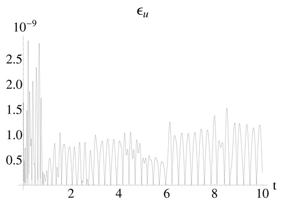
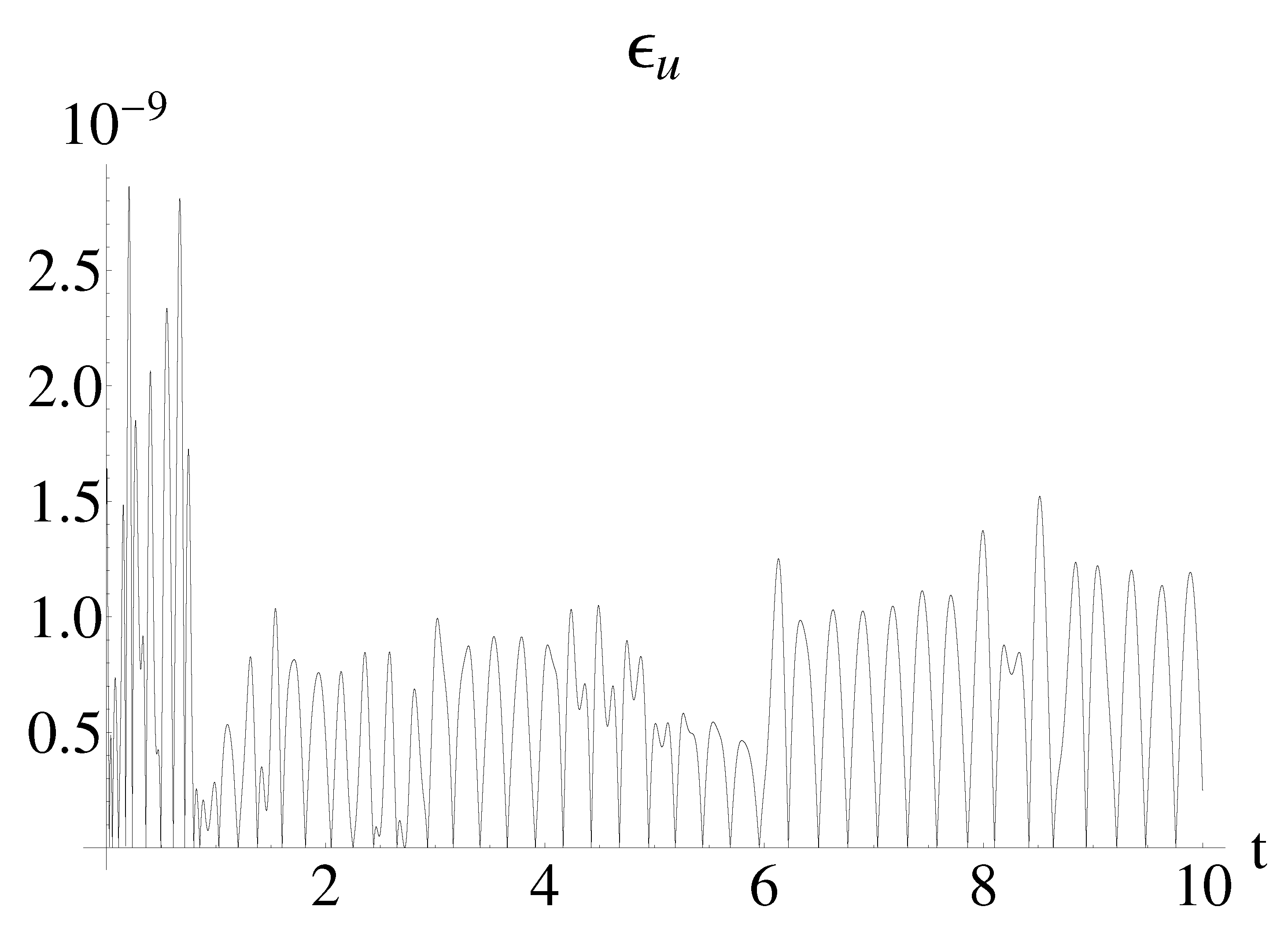
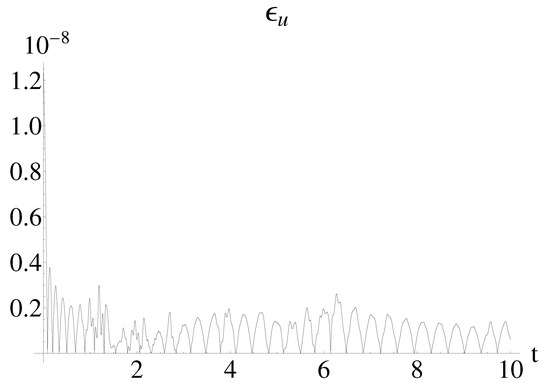
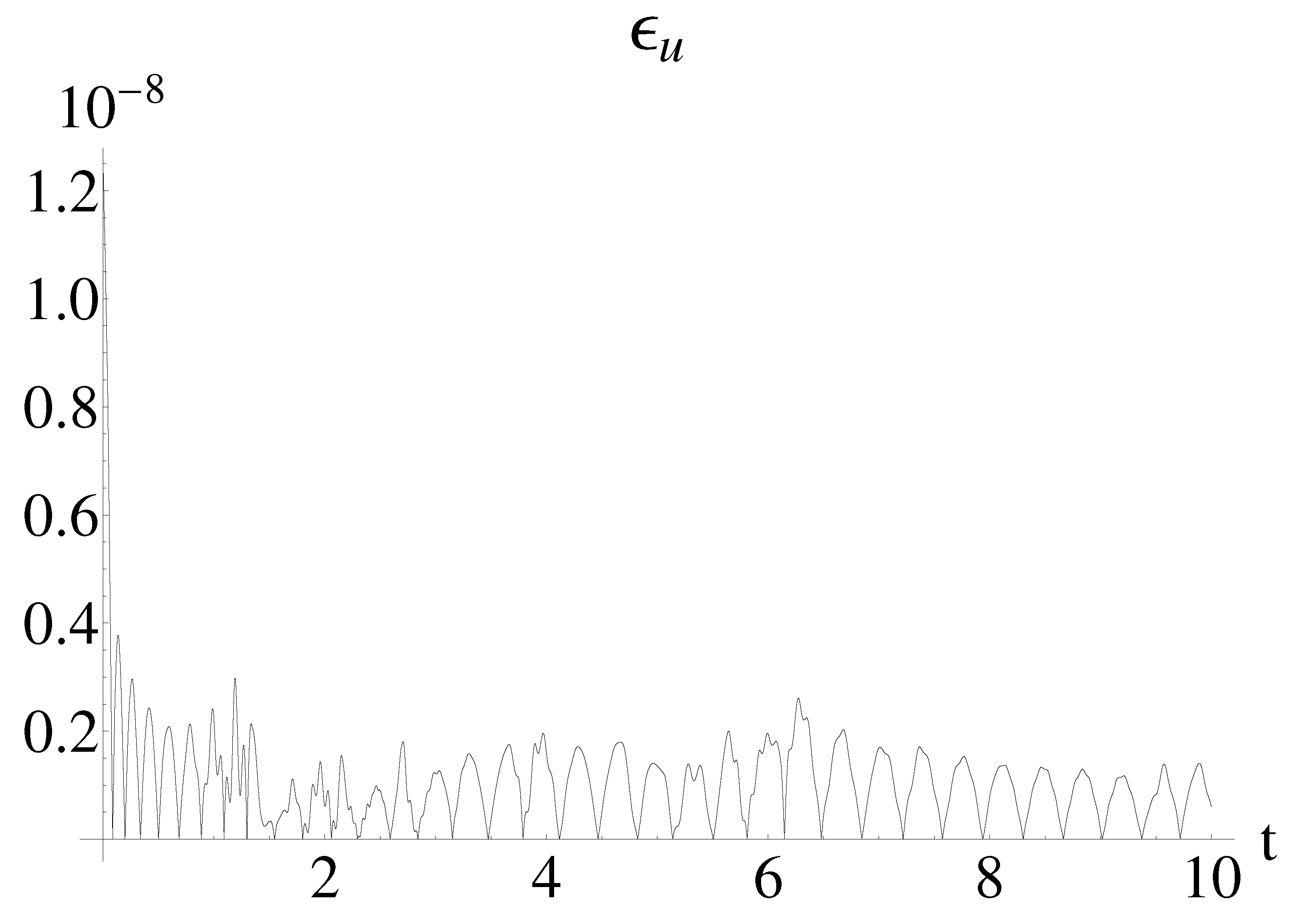
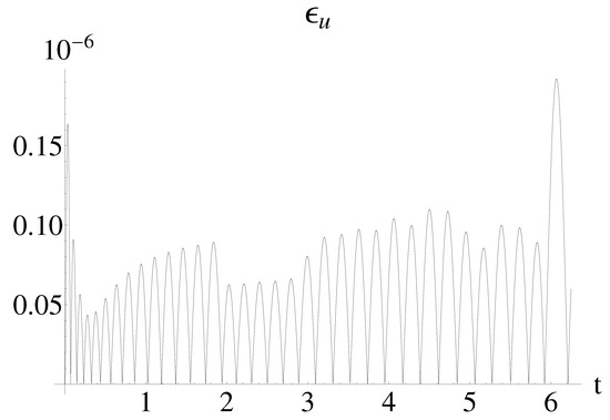
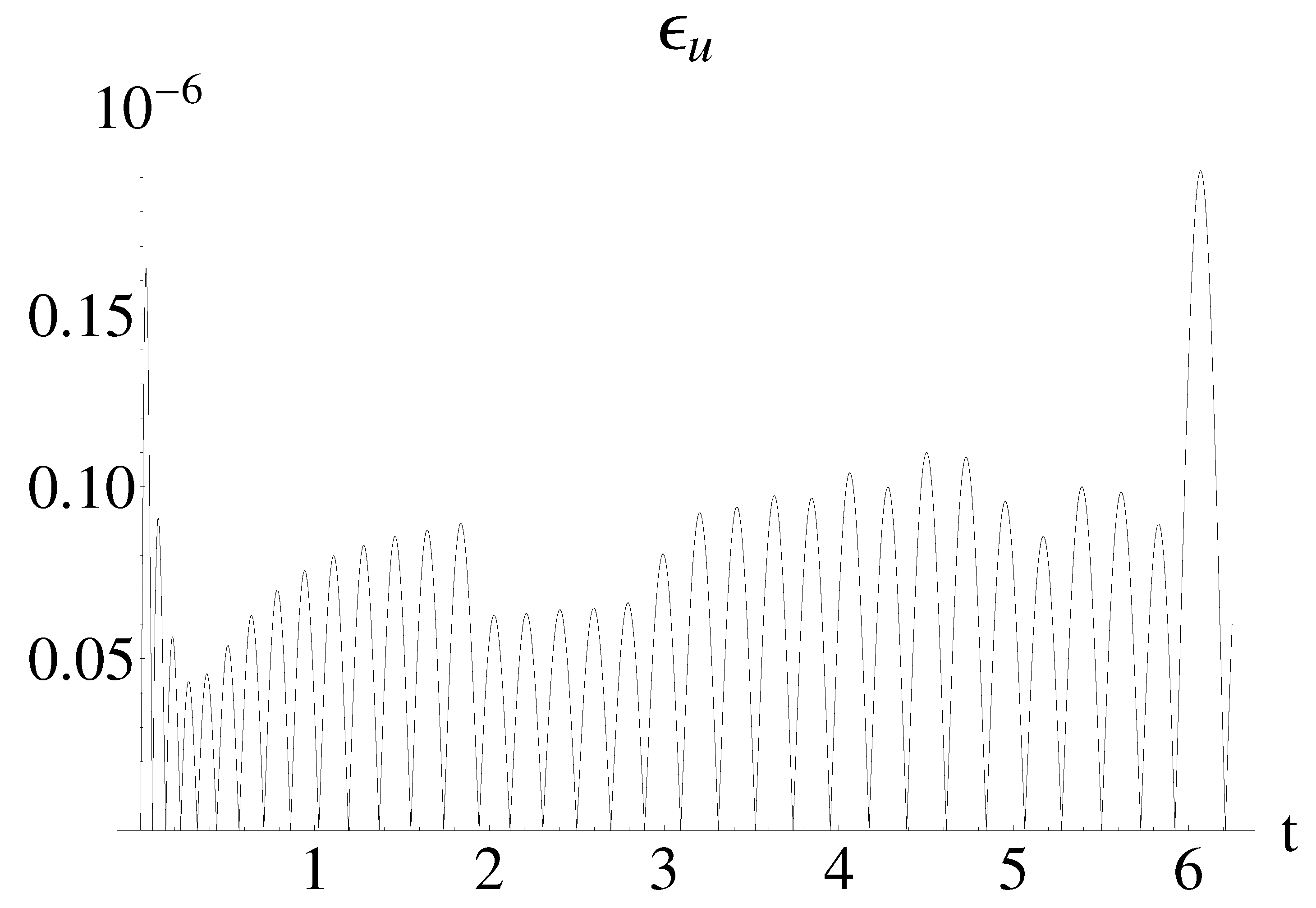
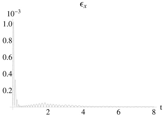
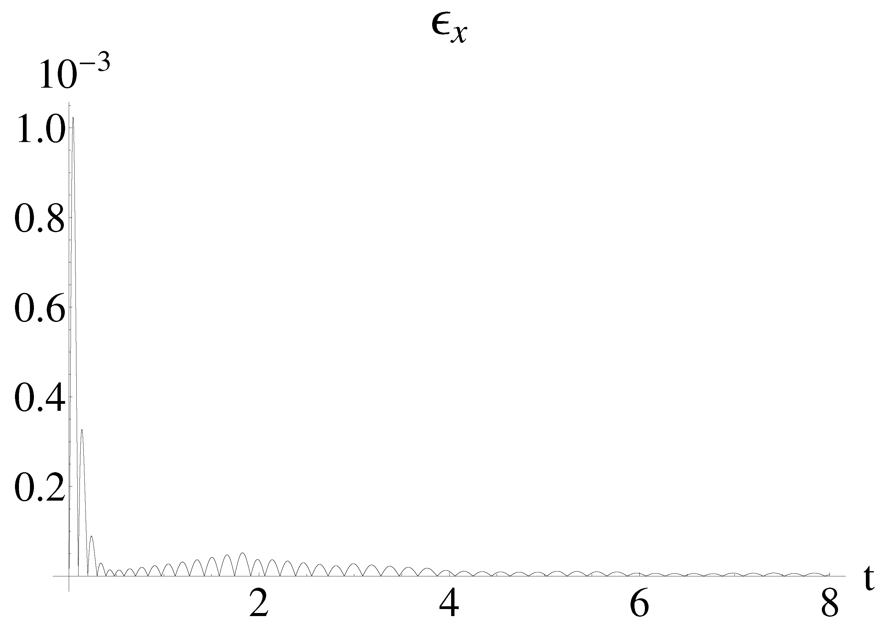
The absolute errors, ${ϵ}_u=|u_{numerical}-{\overline{u}}_{OAFM}|$, represented in Figure 1 and quantitative presented in Table 1 show the accuracy of the analytical solutions by comparison with the numerical one.

Figure 1. Variation of the function: ${ϵ}_u=|u_{numerical}-{\overline{u}}_{OAFM}|$ for: $x_0=0.85$, $y_0=0.25$, $z_0=0.45$, physical constants: $a=b=0$, $c=0.75$ and index $N_{max}=15$; ${\overline{u}}_{OAFM}$ using Equations (48) and (A3).

Table 1. Values of the function: ${ϵ}_u=|u_{numerical}-{\overline{u}}_{OAFM}|$ for: $x_0=0.85$, $y_0=0.25$, $z_0=0.45$, physical constants: $a=b=0$, $c=0.75$ and three values of the index $N_{max}$; ${\overline{u}}_{OAFM}$ using Equations (6), (48) and (A1)–(A3).

t	${\mathit{ϵ}}_{\mathit{u}}:$ ${\mathit{N}}_{\mathit{max}}=5$	${\mathit{ϵ}}_{\mathit{u}}:$ ${\mathit{N}}_{\mathit{max}}=10$	${\mathit{ϵ}}_{\mathit{u}}:$ ${\mathit{N}}_{\mathit{max}}=15$
0	1.1657 $\times {10}^{-15}$	1.8318 $\times {10}^{-15}$	1.9595 $\times {10}^{-14}$
2/3	4.1012 $\times {10}^{-6}$	3.2076 $\times {10}^{-9}$	2.7915 $\times {10}^{-9}$
4/3	9.6432 $\times {10}^{-6}$	9.8827 $\times {10}^{-10}$	7.2826 $\times {10}^{-10}$
2	3.6433 $\times {10}^{-6}$	6.0719 $\times {10}^{-10}$	4.7792 $\times {10}^{-10}$
8/3	1.5454 $\times {10}^{-6}$	1.2850 $\times {10}^{-10}$	1.0486 $\times {10}^{-10}$
10/3	3.4423 $\times {10}^{-6}$	5.7415 $\times {10}^{-10}$	7.8414 $\times {10}^{-10}$
4	1.7789 $\times {10}^{-6}$	3.7951 $\times {10}^{-11}$	8.2441 $\times {10}^{-10}$
14/3	1.1840 $\times {10}^{-6}$	7.0023 $\times {10}^{-10}$	2.5738 $\times {10}^{-10}$
16/3	2.2333 $\times {10}^{-6}$	9.9519 $\times {10}^{-10}$	4.9712 $\times {10}^{-10}$
6	3.8233 $\times {10}^{-6}$	1.8927 $\times {10}^{-9}$	2.6078 $\times {10}^{-10}$
20/3	7.4571 $\times {10}^{-6}$	7.6619 $\times {10}^{-10}$	9.3054 $\times {10}^{-10}$
22/3	5.2065 $\times {10}^{-6}$	7.9709 $\times {10}^{-10}$	3.0844 $\times {10}^{-10}$
8	2.7205 $\times {10}^{-6}$	1.2988 $\times {10}^{-9}$	1.3709 $\times {10}^{-9}$
26/3	9.6892 $\times {10}^{-6}$	1.1629 $\times {10}^{-9}$	2.3837 $\times {10}^{-10}$
28/3	3.8050 $\times {10}^{-6}$	7.1915 $\times {10}^{-10}$	1.1698 $\times {10}^{-9}$
10	6.8606 $\times {10}^{-6}$	1.7138 $\times {10}^{-9}$	2.4809 $\times {10}^{-10}$

As the value of $N_{max}$ index increases, the magnitude of the difference ${ϵ}_u=|u_{numerical}-{\overline{u}}_{OAFM}|$ decreases to ${10}^{-10}$, as shown in Table 1.

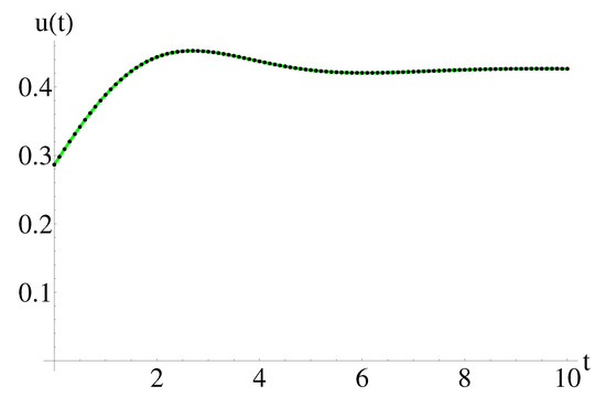
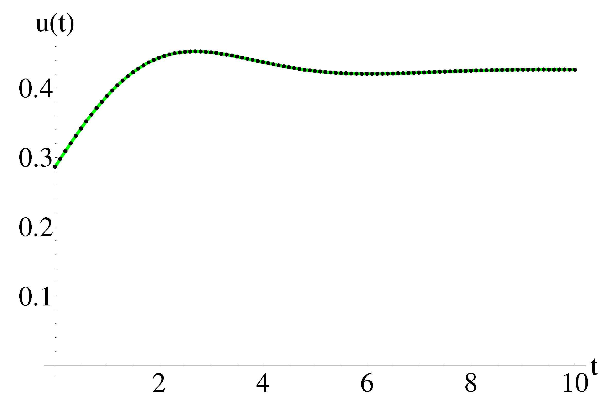
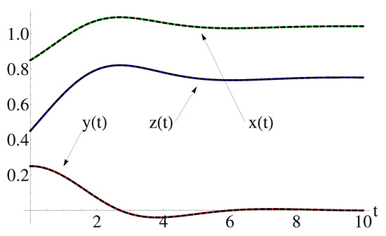
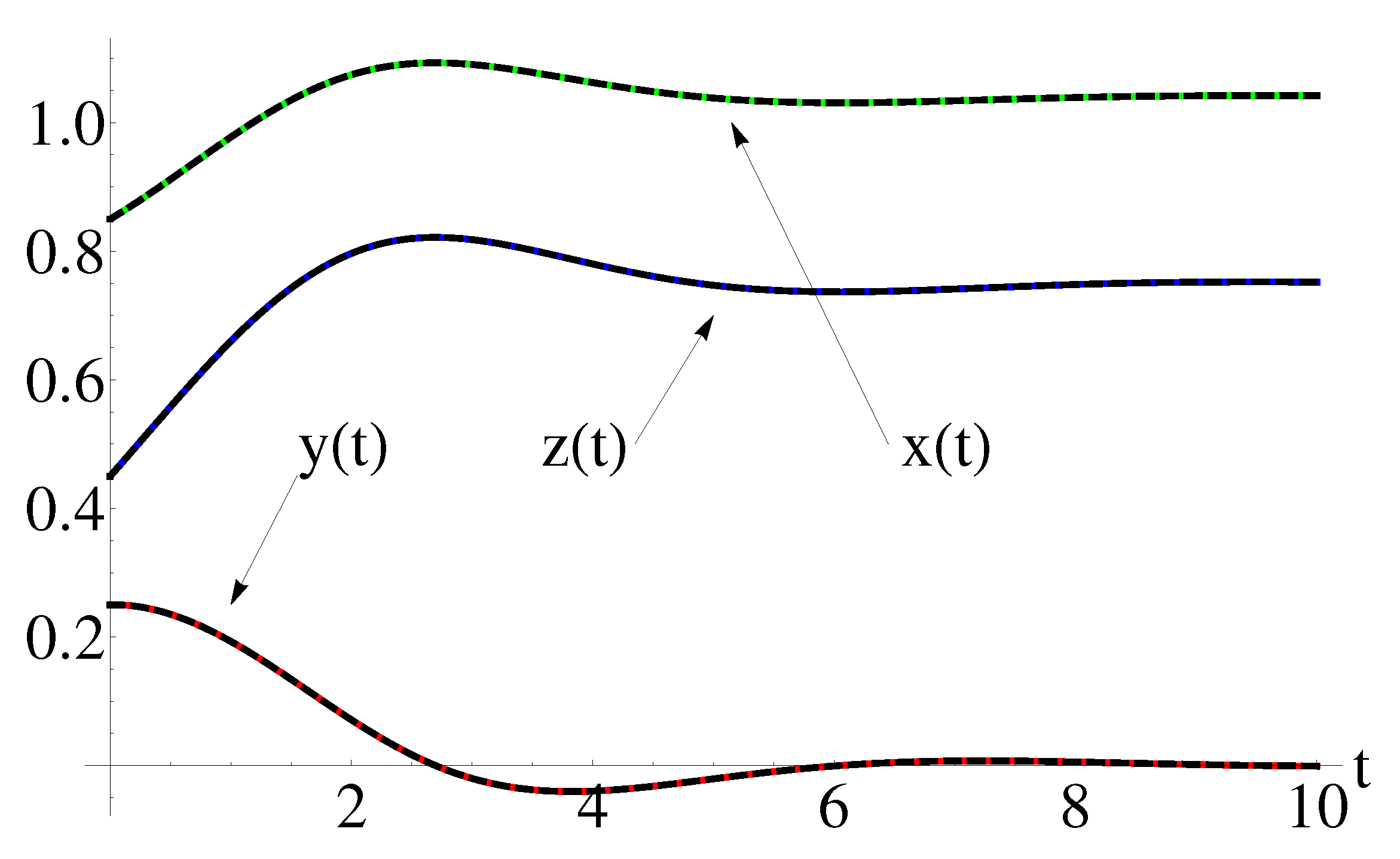
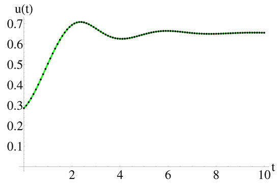
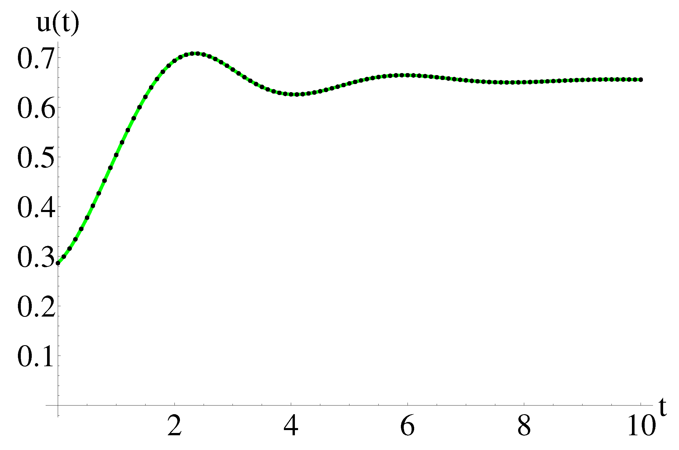
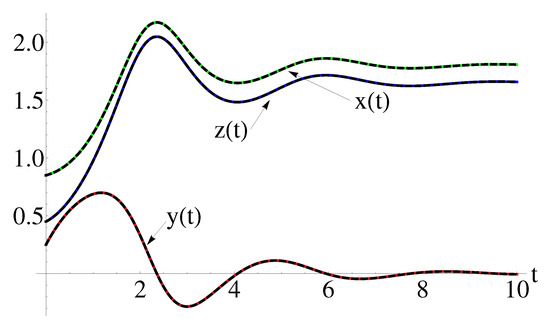
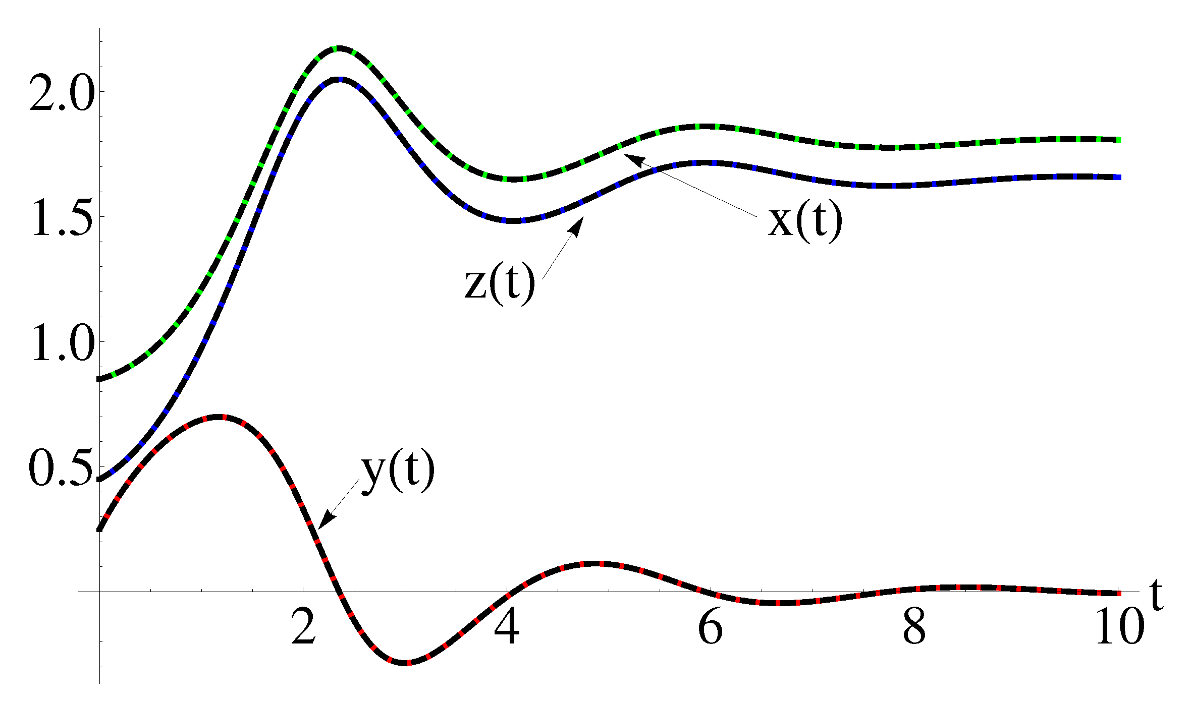
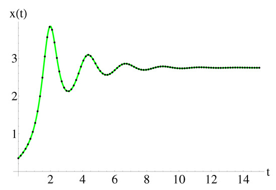
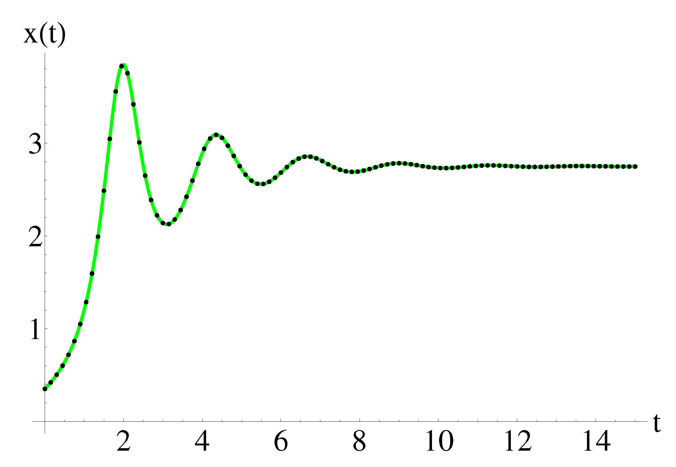
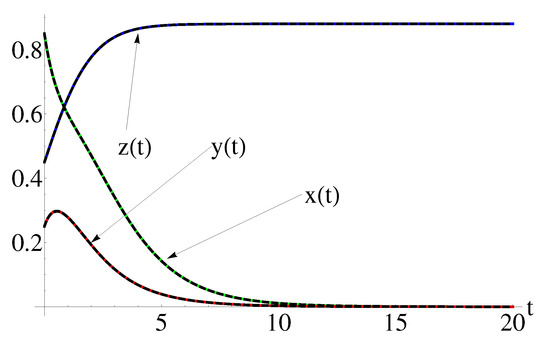
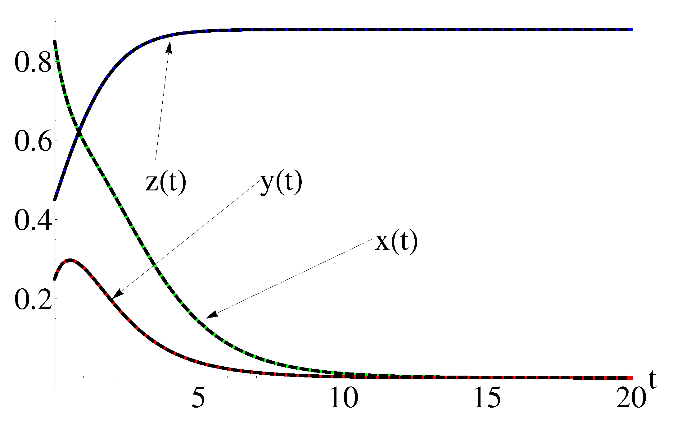
The OAFM scheme is validated in the first case for the initial conditions: $x_0=0.85$, $y_0=0.25$, $z_0=0.45$, and physical parameters: $a=b=0$, $c=0.75$. The profiles of the functions ${\overline{u}}_{OAFM}$, $({\overline{x}}_{OAFM},{\overline{y}}_{OAFM},{\overline{z}}_{OAFM})$ are depicted in Figure 2 and Figure 3.

Figure 2. The performance of the approximate solution ${\overline{u}}_{OAFM}$ using Equations (6), (48) and (A3) for: $x_0=0.85$, $y_0=0.25$, $z_0=0.45$, physical constants: $a=b=0$, $c=0.75$ and index $N_{max}=15$ by comparison with numerical integration: OAFM solution (dotted black curve) and numerical results (solid green curve), respectively.

Figure 3. The performance of the approximate solutions $({\overline{x}}_{OAFM},{\overline{y}}_{OAFM},{\overline{z}}_{OAFM})$ given by Equations (5) using Equation (A3) for: $x_0=0.85$, $y_0=0.25$, $z_0=0.45$, physical constants: $a=b=0$, $c=0.75$ and index $N_{max}=15$ by comparison with numerical integration: OAFM solution (dashing black curve) and numerical results (solid color curve: green curve for $x\left(t\right)$, red curve for $y\left(t\right)$, blue curve for $z\left(t\right)$), respectively.

The comparison between the functions: ${\overline{u}}_{OAFM}$, $({\overline{x}}_{OAFM},{\overline{y}}_{OAFM},{\overline{z}}_{OAFM})$ and corresponding numerical ones, respectively, is shown in Table 2, Figure 2 and Figure 3, respectively.

Table 2. Values of the function ${\overline{u}}_{OAFM}$ of Equation (6) using Equations (48) and (A3) and numerical integration for: $x_0=0.85$, $y_0=0.25$, $z_0=0.45$, physical constants: $a=b=0$, $c=0.75$ and index $N_{max}=15$; (absolute errors: ${ϵ}_u=|u_{numerical}-{\overline{u}}_{OAFM}|$).

t	${\mathit{u}}_{\mathit{numerical}}$	${\overline{\mathit{u}}}_{\mathit{OAFM}}$	${\mathit{ϵ}}_{\mathit{u}}$
0	0.2864216553	0.2864216553	1.9595 $\times {10}^{-14}$
2/3	0.3584973463	0.3584973491	2.7915 $\times {10}^{-9}$
4/3	0.4129149530	0.4129149523	7.2826 $\times {10}^{-10}$
2	0.4436536490	0.4436536495	4.7792 $\times {10}^{-10}$
8/3	0.4528209765	0.4528209766	1.0486 $\times {10}^{-10}$
10/3	0.4478622144	0.4478622152	7.8414 $\times {10}^{-10}$
4	0.4374518771	0.4374518763	8.2441 $\times {10}^{-10}$
14/3	0.4279771942	0.4279771939	2.5738 $\times {10}^{-10}$
16/3	0.4223125003	0.4223125008	4.9712 $\times {10}^{-10}$
6	0.4205486947	0.4205486945	2.6078 $\times {10}^{-10}$
20/3	0.4213838309	0.4213838300	9.3054 $\times {10}^{-10}$
22/3	0.4232754956	0.4232754959	3.0844 $\times {10}^{-10}$
8	0.4250788743	0.4250788757	1.3709 $\times {10}^{-9}$
26/3	0.4262334393	0.4262334390	2.3837 $\times {10}^{-10}$
28/3	0.4266668422	0.4266668410	1.1698 $\times {10}^{-9}$
10	0.4265838588	0.4265838586	2.4809 $\times {10}^{-10}$

The OAFM procedure does not depend on the existence of the small parameters. For example, in the case $1<c<2$, the semi-analytical solutions are deduced and are tabular and graphically presented in Table 3, Table 4 and the Figure 4, Figure 5, Figure 6, respectively.

Table 3. Values of the function ${\overline{u}}_{OAFM}$ of Equation (6) using Equations (48) and (A4) and numerical integration for: $x_0=0.85$, $y_0=0.25$, $z_0=0.45$, physical constants: $a=b=0$, $c=1.65$ and index $N_{max}=15$; (absolute errors: ${ϵ}_u=|u_{numerical}-{\overline{u}}_{OAFM}|$).

t	${\mathit{u}}_{\mathit{numerical}}$	${\overline{\mathit{u}}}_{\mathit{OAFM}}$	${\mathit{ϵ}}_{\mathit{u}}$
0	0.2864216553	0.2864216553	2.6090 $\times {10}^{-15}$
1	0.5040475185	0.5040475163	2.1994 $\times {10}^{-9}$
2	0.6935084245	0.6935084239	6.1016 $\times {10}^{-10}$
3	0.6759260268	0.6759260256	1.2135 $\times {10}^{-9}$
4	0.6259218284	0.6259218300	1.5863 $\times {10}^{-9}$
5	0.6479393233	0.6479393220	1.3531 $\times {10}^{-9}$
6	0.6644385350	0.6644385369	1.9491 $\times {10}^{-9}$
7	0.6541680149	0.6541680132	1.6891 $\times {10}^{-9}$
8	0.6504024564	0.6504024572	7.8691 $\times {10}^{-10}$
9	0.6550117518	0.6550117520	1.6849 $\times {10}^{-10}$
10	0.6555626630	0.6555626624	6.0246 $\times {10}^{-10}$

Table 4. Values of the function ${\overline{x}}_{OAFM}$ of Equation (14) using Equations (2), (48) and (A5) and numerical integration for: $x_0=0.35$, $y_0=1.25$, $z_0=0.35$, physical constants: $a=b=0$, $c=0.75$ and index $N_{max}=15$; (absolute errors: ${ϵ}_x=|x_{numerical}-{\overline{x}}_{OAFM}|$).

t	${\mathit{x}}_{\mathit{numerical}}$	${\overline{\mathit{x}}}_{\mathit{OAFM}}$	${\mathit{ϵ}}_{\mathit{x}}$
0	0.35	0.3500000000	3.2196 $\times {10}^{-15}$
4/5	0.7180947406	0.7180946733	6.7311 $\times {10}^{-8}$
8/5	0.9894075244	0.9894075888	6.4390 $\times {10}^{-8}$
12/5	1.0329783203	1.0329783845	6.4131 $\times {10}^{-8}$
16/5	0.9337078340	0.9337079263	9.2338 $\times {10}^{-8}$
4	0.8295122786	0.8295123449	6.6299 $\times {10}^{-8}$
24/5	0.7643086881	0.7643086284	5.9701 $\times {10}^{-8}$
28/5	0.7331060653	0.7331059690	9.6249 $\times {10}^{-8}$
32/5	0.7233040955	0.7233040346	6.0894 $\times {10}^{-8}$
36/5	0.7249206645	0.7249199218	7.4270 $\times {10}^{-7}$
8	0.7313261823	0.7313156100	1.0572 $\times {10}^{-5}$

Figure 4. Variation of the function: ${ϵ}_u=|u_{numerical}-{\overline{u}}_{OAFM}|$ for: $x_0=0.85$, $y_0=0.25$, $z_0=0.45$, physical constants: $a=b=0$, $c=1.65$ and index $N_{max}=15$ by comparison with numerical integration; ${\overline{u}}_{OAFM}$ using Equations (48) and (A4).

Figure 5. The performance of the approximate solution ${\overline{u}}_{OAFM}$ using Equations (6), (48) and (A4) for: $x_0=0.85$, $y_0=0.25$, $z_0=0.45$, physical constants: $a=b=0$, $c=1.65$ and index $N_{max}=15$ by comparison with numerical integration: OAFM solution (dotted black curve) and numerical results (solid green curve), respectively.

Figure 6. The performance of the approximate solutions $({\overline{x}}_{OAFM},{\overline{y}}_{OAFM},{\overline{z}}_{OAFM})$ given by Equations (5) using Equation (A4) for: $x_0=0.85$, $y_0=0.25$, $z_0=0.45$, physical constants: $a=b=0$, $c=1.65$ and index $N_{max}=15$ by comparison with numerical integration: OAFM solution (dashing black curve) and numerical results (solid color curve: green curve for $x\left(t\right)$, red curve for $y\left(t\right)$, blue curve for $z\left(t\right)$), respectively.

4.2. Case 2: $a=0$, $b=0$, $c>0$, $x^2\left(0\right)-z^2\left(0\right)=0$

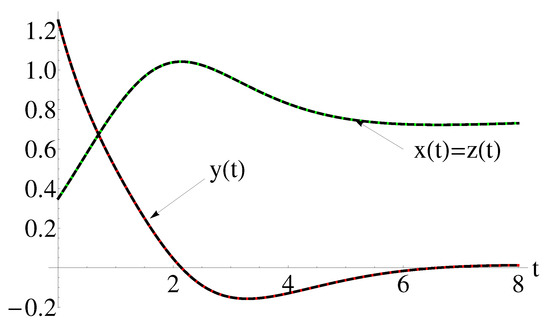
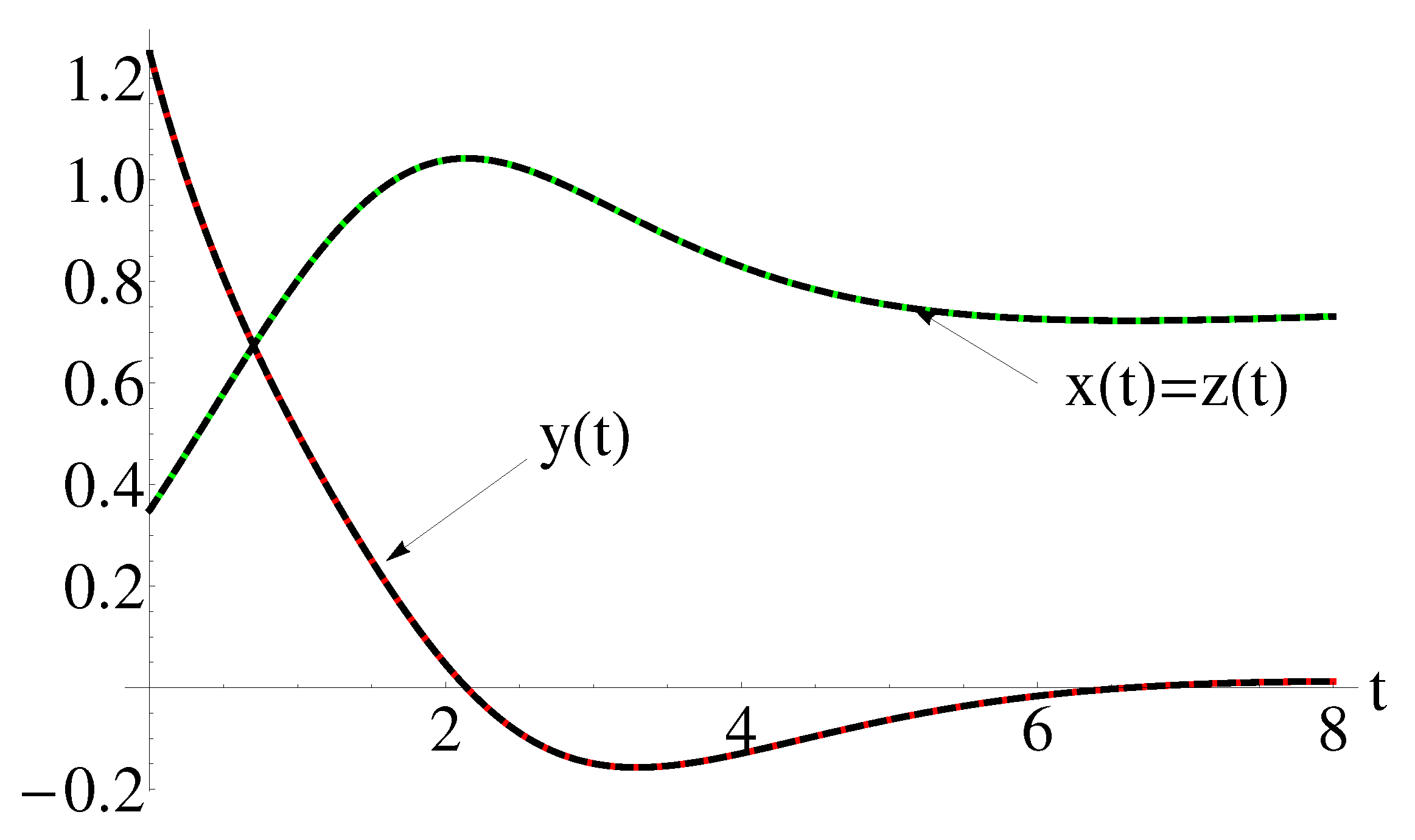
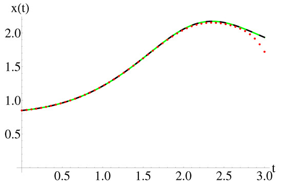
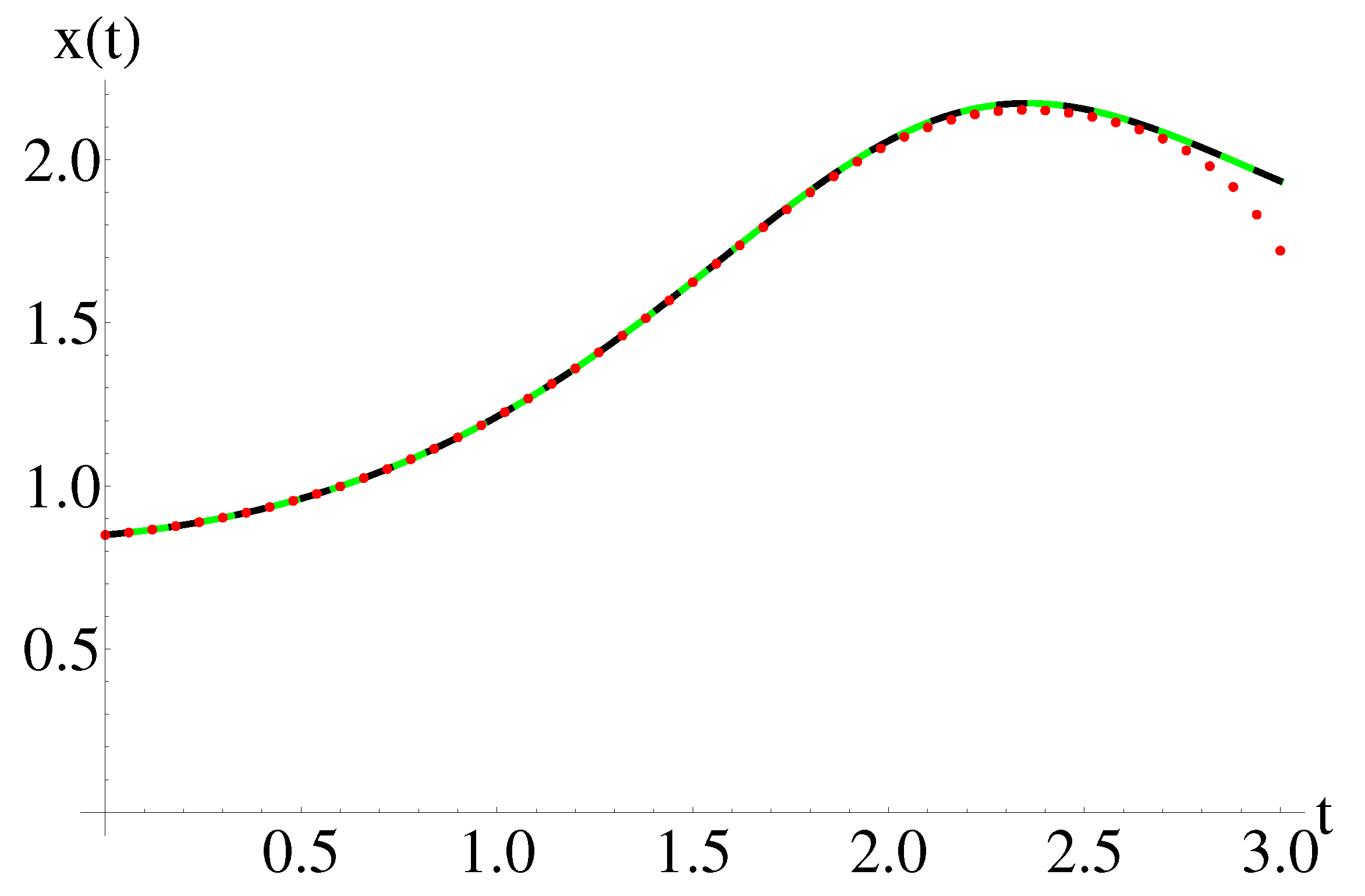
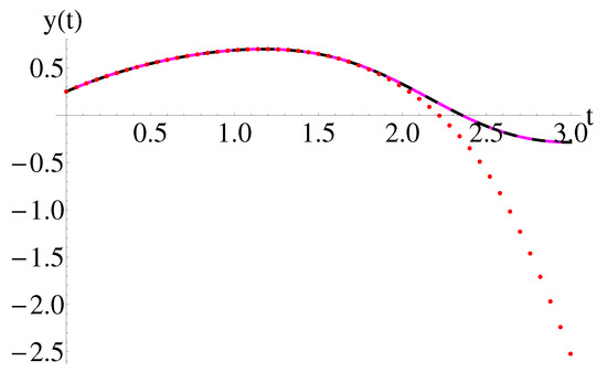
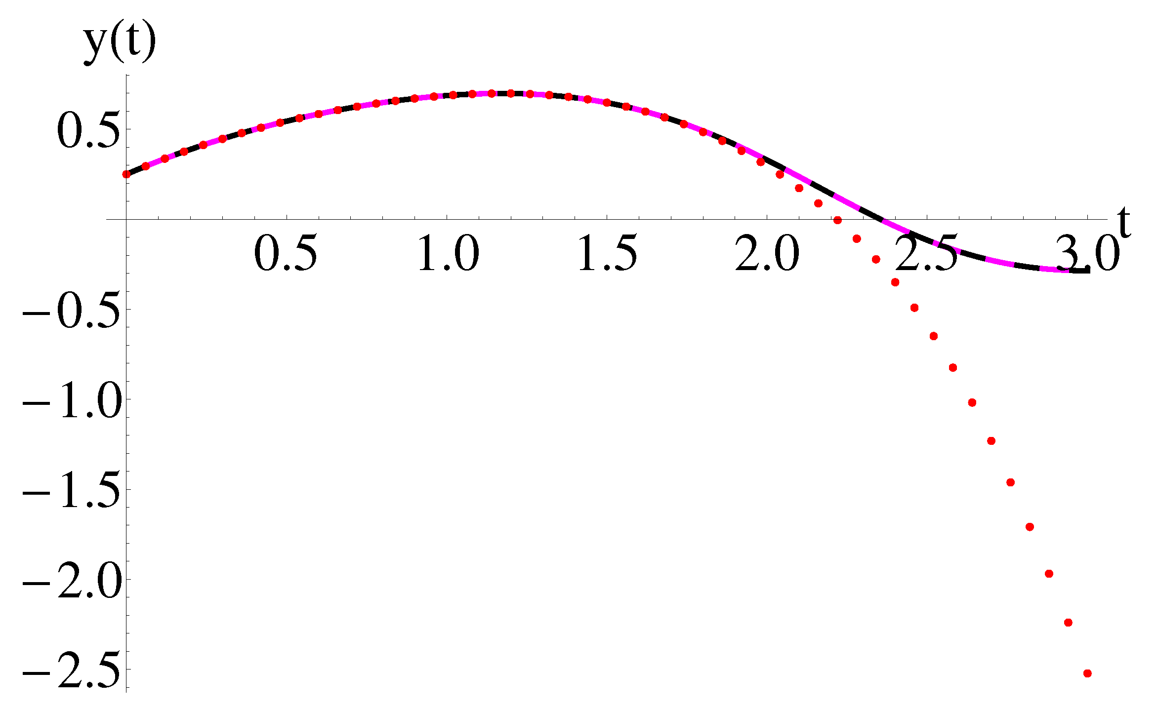
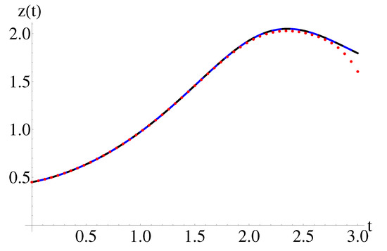
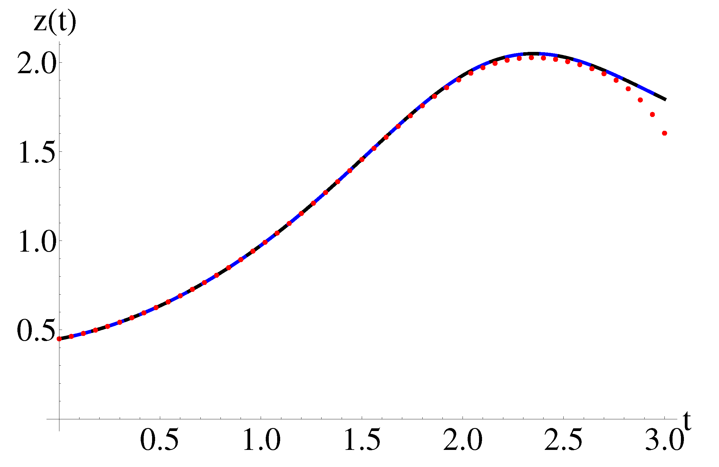
This special case is graphically and tabular validated in the Table 5 and the Figure 7 and Figure 8 for $0<c<1$, and the Figure 9, Figure 10 for $1<c$, respectively.

Table 5. Values of the function ${\overline{x}}_{OAFM}$ of Equation (14) using Equations (2) and (53) and numerical integration for: $x_0=0.35$, $y_0=1.25$, $z_0=0.35$, physical constants: $a=b=0$, $c=2.75$ and index $N_{max}=10$; (absolute errors: ${ϵ}_x=|x_{numerical}-{\overline{x}}_{OAFM}|$).

t	${\mathit{x}}_{\mathit{numerical}}$	${\overline{\mathit{x}}}_{\mathit{OAFM}}$	${\mathit{ϵ}}_{\mathit{x}}$
0	0.35	0.3499999999	1.2277 $\times {10}^{-12}$
1.5	2.4864220472	2.4864638876	4.1840 $\times {10}^{-5}$
3	2.1391432618	2.1391155963	2.7665 $\times {10}^{-5}$
4.5	3.0586602034	3.0586525321	7.6713 $\times {10}^{-6}$
6	2.6828701214	2.6828761797	6.0582 $\times {10}^{-6}$
7.5	2.7140619767	2.7140597707	2.2059 $\times {10}^{-6}$
9	2.7834528538	2.7834520693	7.8444 $\times {10}^{-7}$
10.5	2.7383390063	2.7383327787	6.2275 $\times {10}^{-6}$
12	2.7492096303	2.7492101388	5.0851 $\times {10}^{-7}$
13.5	2.7530354979	2.7530279196	7.5783 $\times {10}^{-6}$
15	2.7484212404	2.7484251614	3.9209 $\times {10}^{-6}$

Figure 7. Variation of the function: ${ϵ}_x=|x_{numerical}-{\overline{x}}_{OAFM}|$ for: $x_0=0.35$, $y_0=1.25$, $z_0=0.35$, physical constants: $a=b=0$, $c=0.75$ and index $N_{max}=15$ by comparison with numerical integration; ${\overline{x}}_{OAFM}$ using Equations (48) and (A5).

Figure 8. The performance of the approximate solutions $({\overline{x}}_{OAFM},{\overline{y}}_{OAFM},{\overline{z}}_{OAFM})$ using Equations (2), (48) and (A5) for: $x_0=0.35$, $y_0=1.25$, $z_0=0.35$, physical constants: $a=b=0$, $c=0.75$ and index $N_{max}=15$ by comparison with numerical integration: OAFM solution (dashing black curve) and numerical results (solid color curve: green curve for $x\left(t\right)$, red curve for $y\left(t\right)$, green curve for $z\left(t\right)$), respectively.

Figure 9. Variation of the function: ${ϵ}_x=|x_{numerical}-{\overline{x}}_{OAFM}|$ for: $x_0=0.35$, $y_0=1.25$, $z_0=0.35$, physical constants: $a=b=0$, $c=2.75$ and index $N_{max}=10$ by comparison with numerical integration; ${\overline{x}}_{OAFM}$ using Equations (53) and (A6).

Figure 10. The performance of the approximate solution ${\overline{x}}_{OAFM}$ using Equations (2), (53) and (A6) for: $x_0=0.35$, $y_0=1.25$, $z_0=0.35$, physical constants: $a=b=0$, $c=2.75$ and index $N_{max}=10$ by comparison with numerical integration: OAFM solution (dotted black curve) and numerical results (solid green curve), respectively.

For initial conditions $x_0=0.35$, $y_0=1.25$, $z_0=0.35$, physical parameters $a=b=0$, $c=2.75$, with $N_{max}=25$, the analytical solution given by Equation (17) is:

$$\begin{array}{c}{\overline{y}}_{OAFM}\left(t\right)=Y\left({\overline{x}}_{OAFM}\left(t\right)\right)=1.3683354447+0.3636494834(2.75-\overline{x})\hfill \\ -0.2996593392{(2.75-\overline{x})}^2+0.0853082757{(2.75-\overline{x})}^3-0.0799849296{(2.75-\overline{x})}^4\hfill \\ +0.1663822321{(2.75-\overline{x})}^5-0.4147645189{(2.75-\overline{x})}^6+0.7964229844{(2.75-\overline{x})}^7\hfill \\ -1.0801299362{(2.75-\overline{x})}^8+0.9943286550{(2.75-\overline{x})}^9-0.5672669223{(2.75-\overline{x})}^{10}\hfill \\ +0.1379029946{(2.75-\overline{x})}^{11}+0.0424445100{(2.75-\overline{x})}^{12}-0.0321713744{(2.75-\overline{x})}^{13}\hfill \\ -0.0029515235{(2.75-\overline{x})}^{14}+0.0055943607{(2.75-\overline{x})}^{15}+0.0005349833{(2.75-\overline{x})}^{16}\hfill \\ -0.0009538447{(2.75-\overline{x})}^{17}-0.0001632209{(2.75-\overline{x})}^{18}+0.0001603915{(2.75-\overline{x})}^{19}\hfill \\ +0.0000421271{(2.75-\overline{x})}^{20}-0.0000292599{(2.75-\overline{x})}^{21}-7.618049\times {10}^{-6}{(2.75-\overline{x})}^{22}\hfill \\ +7.621279\times {10}^{-6}{(2.75-\overline{x})}^{23}-1.804665\times {10}^{-6}{(2.75-\overline{x})}^{24}+1.476849\times {10}^{-7}{(2.75-\overline{x})}^{25},\hfill \end{array}$$

(58)

where $\overline{x}\left(t\right)={\overline{x}}_{OAFM}\left(t\right)$ is given by Equations (53) and (A6).

4.3. Case 3: $a=1$, $b=0$, $c=1$

This special case is graphically validated in the Figure 11. The obtained semi-analytical solutions have asymptotic behaviors.

Figure 11. The performance of the approximate solutions $({\overline{x}}_{OAFM},{\overline{y}}_{OAFM},{\overline{z}}_{OAFM})$ using Equations (A7)–(A9) for: $x_0=0.85$, $y_0=0.25$, $z_0=0.45$, physical constants: $a=c=1$, $b=0$ by comparison with numerical integration: OAFM solution (dashing black curve) and numerical results (solid color curve: green line for $x\left(t\right)$, red curve for $y\left(t\right)$, blue curve for $z\left(t\right)$), respectively.

4.4. OAFM Versus Iterative Solutions

The advantage of the OAFM method by comparison with the iterative method described in [25] (using six iterations) is highlighted in this subsection. In Table 6 and Figure 12, Figure 13, Figure 14, respectively, can the precision and efficiency of the OAFM method be seen.

Table 6. Values of the approximate solution ${\overline{y}}_{OAFM}\left(t\right)$ (A3), the iterative solution $y_{iter}\left(t\right)$ and the numerical integration.

t	${\mathit{y}}_{\mathit{numerical}}$	${\overline{\mathit{y}}}_{\mathit{OAFM}}$	${\mathit{y}}_{\mathit{iter}}$
0	0.25	0.2500002178	0.25
3/10	0.4470695733	0.4470696593	0.4470696162
3/5	0.5851841885	0.5851841406	0.5851868094
9/10	0.6710767215	0.6710767528	0.6711282196
6/5	0.6989510553	0.6989513115	0.6992972483
3/2	0.6477917304	0.6477918153	0.6484557561
9/5	0.4914772579	0.4914772816	0.4851905665
21/10	0.2365556519	0.2365555430	0.1730570170
12/5	−0.0390106618	−0.0390108032	−0.3495996952
27/10	−0.2277288212	−0.2277287883	−1.2307821890
3	−0.2852949370	−0.2852948869	−2.5227962146

Figure 12. The performance of the approximate solution ${\overline{x}}_{OAFM}\left(t\right)$ of Equation (3) using Equation (A3) (dashing black curve), by comparison with the iterative solution $x_{iter}\left(t\right)$ using Equation (61) (dotted red curve) and the corresponding numerical ones (solid color curve), respectively.

Figure 13. The performance of the approximate solution ${\overline{y}}_{OAFM}\left(t\right)$ of Equation (3) using Equation (A3) (dashing black curve), by comparison with the iterative solution $y_{iter}\left(t\right)$ using Equation (61) (dotted red curve) and the corresponding numerical ones (solid color curve), respectively.

Figure 14. The performance of the approximate solution ${\overline{z}}_{OAFM}\left(t\right)$ of Equation (3) using Equation (A3) (dashing black curve), by comparison with the iterative solution $z_{iter}\left(t\right)$ using Equation (61) (dotted red curve) and the corresponding numerical ones (solid color curve), respectively.

The iterative method presented in [25] is applied.

By integration of the system (3) is integrated over the interval $[0,t]$, it obtains:

$$\begin{array}{c}{\displaystyle x\left(t\right)=x\left(0\right)+\underset{0}{\overset{t}{\int }}y\left(s\right)z\left(s\right)ds}\hfill \\ {\displaystyle y\left(t\right)=y\left(0\right)+\underset{0}{\overset{t}{\int }}\left(cx\left(s\right)-y\left(s\right)-x\left(s\right)z\left(s\right)\right)ds}\hfill \\ {\displaystyle z\left(t\right)=z\left(0\right)+\underset{0}{\overset{t}{\int }}x\left(s\right)y\left(s\right)ds}\hfill \end{array}.$$

(59)

The iterative algorithm leads to:

$$\begin{array}{c}{\displaystyle x_0\left(t\right)=x\left(0\right),x_1\left(t\right)=N_1(x_0,y_0,z_0)=\underset{0}{\overset{t}{\int }}y\left(0\right)z\left(0\right)ds,}\hfill \\ {\displaystyle y_0\left(t\right)=y\left(0\right),y_1\left(t\right)=N_2(x_0,y_0,z_0)=\underset{0}{\overset{t}{\int }}\left(cx\left(0\right)-y\left(0\right)-x\left(0\right)z\left(0\right)\right)ds,}\hfill \\ {\displaystyle z_0\left(t\right)=z\left(0\right),z_1\left(t\right)=N_3(x_0,y_0,z_0)=\underset{0}{\overset{t}{\int }}x\left(0\right)y\left(0\right)ds,}\hfill \\ \cdots \hfill \\ x_m\left(t\right)=N_1\left({\displaystyle \sum _{i=0}^{m-1}{x}_i,\sum _{i=0}^{m-1}{y}_i,\sum _{i=0}^{m-1}{z}_i}\right)-N_1\left({\displaystyle \sum _{i=0}^{m-2}{x}_i,\sum _{i=0}^{m-2}{y}_i,\sum _{i=0}^{m-2}{z}_i}\right),\hfill \\ y_m\left(t\right)=N_2\left({\displaystyle \sum _{i=0}^{m-1}{x}_i,\sum _{i=0}^{m-1}{y}_i,\sum _{i=0}^{m-1}{z}_i}\right)-N_2\left({\displaystyle \sum _{i=0}^{m-2}{x}_i,\sum _{i=0}^{m-2}{y}_i,\sum _{i=0}^{m-2}{z}_i}\right),\hfill \\ z_m\left(t\right)=N_3\left({\displaystyle \sum _{i=0}^{m-1}{x}_i,\sum _{i=0}^{m-1}{y}_i,\sum _{i=0}^{m-1}{z}_i}\right)-N_3\left({\displaystyle \sum _{i=0}^{m-2}{x}_i,\sum _{i=0}^{m-2}{y}_i,\sum _{i=0}^{m-2}{z}_i}\right),\hfill \\ m\ge 2.\hfill \end{array}$$

(60)

The iterative algorithm leads to the solution of the Equations (3) as:

$${\displaystyle x_{iter}\left(t\right)=\sum _{m=0}^{\infty }{x}_m\left(t\right),y_{iter}\left(t\right)=\sum _{m=0}^{\infty }{y}_m\left(t\right),z_{iter}\left(t\right)=\sum _{m=0}^{\infty }{z}_m\left(t\right),}$$

For the initial conditions: $x\left(0\right)=0.45$, $y\left(0\right)=0.25$, $z\left(0\right)=0.75$ (presented in Table 6)), the iterative solutions $x_{iter}\left(t\right)$, after six iterations using the algorithm (60), have the form:

$$\begin{array}{c}{\displaystyle x_{iter}\left(t\right)=\sum _{m=0}^6{x}_m\left(t\right)=0.85+0.1125t+0.1998124999t^2+0.0218125t^3}\hfill \\ +0.0521700260t^4-0.0336897018t^5+0.0160002120t^6-0.0070853272t^7\hfill \\ +0.0015970411t^8-0.0012344672t^9+0.0005645053t^{10}-0.0002664156t^{11}\hfill \\ +0.0000790932t^{12}-2.208506\times {10}^{-6}{t}^{13}-3.925096\times {10}^{-6}{t}^{14}+5.506592\times {10}^{-6}{t}^{15}\hfill \\ -3.090922\times {10}^{-6}{t}^{16}+1.881557\times {10}^{-6}{t}^{17}-1.008333\times {10}^{-6}{t}^{18}+\mathcal{O}\left({10}^{-7}\right),\hfill \\ \\ {\displaystyle y_{iter}\left(t\right)=\sum _{m=0}^6{y}_m\left(t\right)=0.25+0.7699999999t-0.4078124999t^2+0.1111885416t^3}\hfill \\ -0.0265884114t^4-0.0039902291t^5-0.0060550019t^6+0.0002670610t^7\hfill \\ +0.0013839553t^8-0.0013333871t^9+0.0007814388t^{10}-0.0002819242t^{11}g\hfill \\ +0.0001425440t^{12}-0.0000702856t^{13}+0.0000337851t^{14}-0.0000150362t^{15}\hfill \\ +4.991647\times {10}^{-6}{t}^{16}-1.743791\times {10}^{-6}{t}^{17}+\mathcal{O}\left({10}^{-7}\right),\hfill \\ {\displaystyle z_{iter}\left(t\right)=\sum _{m=0}^6{z}_m\left(t\right)=0.45+0.2125t+0.3413124999t^2-0.0700208333t^3}\hfill \\ +0.0519850260t^4-0.0123478684t^5+0.0064478423t^6-0.0073910215t^7\hfill \\ +0.0034423047t^8-0.0018261966t^9+0.0004786076t^{10}-0.0001647272t^{11}\hfill \\ +0.0000663721t^{12}-0.0000127163t^{13}-8.862928\times {10}^{-7}{t}^{14}+6.926354\times {10}^{-6}{t}^{15}\hfill \\ -3.987105\times {10}^{-6}{t}^{16}+1.886052\times {10}^{-6}{t}^{17}+\mathcal{O}\left({10}^{-7}\right).\hfill \end{array}$$

(61)

Figure 12, Figure 13 and Figure 14 show the the OAFM solutions ${\overline{x}}_{OAFM}$, ${\overline{y}}_{OAFM}$, ${\overline{z}}_{OAFM}$, by comparison with the corresponding iterative solutions given in Equation (61) and the corresponding numerical ones. This comparison reflects the accuracy of the OAFM approach using only one iteration.

5. Conclusions

The present paper focuses on developing the Optimal Auxiliary Functions Method (OAFM) to derive semi-analytical solutions for the Qi-type dynamical system. The system admits a prime integral (constant of motion), indicating symmetry with respect to the $Oz$-axis. A good agreement between the analytical and numerical results has been demonstrated, reflecting the accuracy of the method.

The following advantages of the OAFM method have been synthesized:

• Effective form of solutions: The flexibility in choosing the linear operator and auxiliary functions allows for an effective form of the solutions.
• Convergence control: The auxiliary functions depend on a finite number of unknown parameters that can be optimally computed to ensure that the residual functions are less than 1, achieving an absolute difference between the semi-analytical and numerical solutions below this threshold.
• No need for small parameters: The semi-analytical solutions are valid for arbitrary values of the physical parameter c, namely for $0<c<1$ and $1<c<2$, respectively.
• Efficiency: The efficiency of the OAFM is highlighted through comparison with corresponding iterative methods. Unlike iterative methods, which require a known exact solution for validation, the OAFM approximates the exact solution by choosing auxiliary functions and optimally determining the unknown parameters, thereby ensuring accuracy.

However, the OAFM has the limitation of not being suitable for complex nonlinear dynamical systems that exhibit chaotic behavior. Additionally, a special case of the Qi-type dynamical system, involving the absence of symmetry, has been investigated, and the exact parametric solution was obtained in power series. Potential practical applications of this system include nonlinear circuits, information storage, encryption, and communication.

References

- Tai, S.; Bu, C.; Wang, Y.; Yue, T.; Liu, H.; Wang, L. Identification of aircraft longitudinal aerodynamic parameters using an online corrective test for wind tunnel virtual flight. Chin. J. Aeronaut. 2024, 37, 261–275. [Google Scholar] [CrossRef] [Scilit]
- Lorenz, E.N. Deterministic nonperiodic flow. J. Atmos. Sci. 1963, 20, 130–141. [Google Scholar] [CrossRef] [Scilit]
- Li, T.-Y.; Yorke, J.A. Period Three Implies Chaos. Am. Math. Mon. 1975, 82, 985–992. [Google Scholar] [CrossRef] [Scilit]
- Rössler, O.E. An Equation for Continuous Chaos. Phys. Lett. A 1976, 57, 397–398. [Google Scholar]
- Rössler, O.E. Continuous chaos, Synergetics: A Workshop. In Proceedings of the International Workshop on Synergetics, Schloss Elmau, Bavaria, 2–7 May 1977; Springer: Berlin/Heidelberg, Germany, 1977; pp. 184–197. [Google Scholar]
- Matsumoto, T.; Chua, L.O.; Tanaka, S. Simplest chaotic nonautonomous circuit. Phys. Rev. A 1984, 30, 1155. [Google Scholar] [CrossRef] [Scilit]
- Chen, G.; Ueta, T. Yet another chaotic attractor. Int. J. Bifurc. Chaos 1999, 9, 1465–1466. [Google Scholar] [CrossRef] [Scilit]
- Lü, J.; Chen, G.; Zhang, S. Dynamical analysis of a new chaotic attractor. Int. J. Bifurc. Chaos 2002, 12, 1001–1015. [Google Scholar]
- Lü, J.; Chen, G.; Cheng, D.; Celikovsky, S. Bridge the gap between the Lorenz system and the Chen system. Int. J. Bifurc. Chaos 2002, 12, 2917–2926. [Google Scholar]
- Sprott, J.C. Some simple chaotic flows. Phys. Rev. E 1994, 50, R647. [Google Scholar] [CrossRef] [Scilit]
- Sprott, J.C. Simplest dissipative chaotic flow. Phys. Lett. A 1997, 228, 271–274. [Google Scholar] [CrossRef] [Scilit]
- Liu, C.; Liu, T.; Liu, L.; Liu, K. A new chaotic attractor. Chaos Solitons Fractals 2004, 22, 1031–1038. [Google Scholar] [CrossRef] [Scilit]
- Van Gorder, R.A.; Choudhury, S.R. Analytical Hopf bifurcation and stability analysis of T system. Commun. Theor. Phys. 2011, 55, 609. [Google Scholar] [CrossRef] [Scilit]
- Yan, S.; Wang, J.; Li, L. Analysis of a new three-dimensional Jerk chaotic system with transient chaos and its adaptive backstepping synchronous control. Integration 2024, 98, 102210. [Google Scholar] [CrossRef] [Scilit]
- Qi, G.; Liang, X. Force Analysis of Qi Chaotic System. Int. J. Bifurc. Chaos 2016, 26, 1650237. [Google Scholar] [CrossRef] [Scilit]
- Li, C.-L.; Xiong, J.-B.; Li, W. A new hyperchaotic system and its generalized synchronization. Optik 2014, 125, 575–579. [Google Scholar] [CrossRef] [Scilit]
- Yang, J.; Feng, Z.; Liu, Z. A New Five-Dimensional Hyperchaotic System with Six Coexisting Attractors. Qual. Theory Dyn. Syst. 2021, 20, 18. [Google Scholar] [CrossRef] [Scilit]
- Zghair, H.K.; Mehdi, S.A.; Sadkhan, S.B. Design and Analytic of A Novel Seven Dimension Hyper Chaotic Systems. In Proceedings of the 1st International Conference of Information Technology to Enhance E-Learning and Other Application 2020, Baghdad, Iraq, 12–13 July 2020. [Google Scholar] [CrossRef] [Scilit]
- Xu, X.; Li, B. Semi-global stabilization of parabolic PDE–ODE systems with input saturation. Automatica 2025, 171, 111931. [Google Scholar] [CrossRef] [Scilit]
- Xu, X.; Li, B. PDE-based observation and predictor-based control for linear systems with distributed infinite input and output delays. Automatica 2024, 170, 111845. [Google Scholar] [CrossRef] [Scilit]
- Marinca, V.; Herisanu, N. Approximate analytical solutions to Jerk equation. In Springer Proceedings in Mathematics 399 & Statistics: Proceedings of the Dynamical Systems: Theoretical and Experimental Analysis, Lodz, Poland, 7–10 December 2015; Springer: Cham, Switzerland, 2016; Volume 182, pp. 169–176. [Google Scholar]
- Marinca, V.; Ene, R.-D.; Marinca, V.B. Optimal Auxiliary Functions Method for viscous flow due to a stretching surface with partial slip. Open Eng. 2018, 8, 261–274. [Google Scholar] [CrossRef] [Scilit]
- Ene, R.-D.; Pop, N.; Lapadat, M. Approximate Closed-Form Solutions for the Rabinovich System via the Optimal Auxiliary Functions Method. Symmetry 2022, 14, 2185. [Google Scholar] [CrossRef] [Scilit]
- Ene, R.-D.; Pop, N.; Lapadat, M.; Dungan, L. Approximate closed-form solutions for the Maxwell-Bloch equations via the Optimal Homotopy Asymptotic Method. Mathematics 2022, 10, 4118. [Google Scholar] [CrossRef] [Scilit]
- Daftardar-Gejji, V.; Jafari, H. An iterative method for solving nonlinear functional equations. J. Math. Anal. Appl. 2006, 316, 753–763. [Google Scholar] [CrossRef] [Scilit]
Disclaimer/Publisher’s Note: The statements, opinions and data contained in all publications are solely those of the individual author(s) and contributor(s) and not of MDPI and/or the editor(s). MDPI and/or the editor(s) disclaim responsibility for any injury to people or property resulting from any ideas, methods, instructions or products referred to in the content. |
© 2024 by the authors. Licensee MDPI, Basel, Switzerland. This article is an open access article distributed under the terms and conditions of the Creative Commons Attribution (CC BY) license (https://creativecommons.org/licenses/by/4.0/).