


Abstract
The spatial variability of soil physicochemical properties significantly influences irrigation efficiency, nutrient availability, and the long-term sustainability of irrigated agriculture in semi-arid regions. This study aimed to quantify and model the spatial distribution of soil properties in a semi-arid irrigation district in central Mexico (Irrigation District 001 “Pabellón de Arteaga”, Aguascalientes), providing spatially explicit information for differential irrigation and fertilization management. Ninety-seven crop and four natural sampling sites were established under a stratified random design at two soil depths (0–30 and 30–60 cm). Geostatistical and machine learning models (Ordinary Kriging, OK; Generalized Additive Models, GAM; and Random Forest, RF) were applied to predict spatial patterns, and their performance was evaluated using statistical metrics. The findings reveal high spatial and vertical variability, with most properties (such as organic matter, total nitrogen, and texture) showing significant stratification with depth. In contrast, others (pH and electrical conductivity, EC) remained remarkably homogeneous vertically. Correlation patterns were identified, highlighting the negative influence of alkaline pH (≈8.0) on the availability of micronutrients (Fe2+ and Mn2+) and the positive association between EC and soluble cations (Ca2+, K+, and Na+). Moran’s Index confirmed significant spatial autocorrelation for most properties, reducing the effective sample size by 30–70%. The comparative evaluation of predictive models demonstrated the superiority of RF over OK and GAMs for predicting chemical properties, thanks to its ability to capture nonlinear relationships and complex interactions. However, the overall predictive performance was moderate, reflecting the multifactorial complexity of the edaphic system. This study lays the foundation for the development of an accessible, low-cost Decision Support System by providing a robust methodological framework for spatial soil characterization and contributing to more sustainable, resilient agriculture, where decision-making is based on quantitative data and predictive models.
1. Introduction
Agriculture is the predominant human activity globally in freshwater consumption, accounting for approximately 70% of total water extraction, primarily for irrigation. In Mexico, this proportion increases to 77%, reflecting the high dependence on irrigation systems in arid and semi-arid regions, which concentrate a substantial share of crop production [1,2]. This intensive demand, coupled with increasing climate variability and climate change, exerts increasing pressure on the sustainability of production systems, especially in contexts where access to and management of water are critical for food security [3].
This problem becomes particularly pressing in north-central Mexico, where the Irrigation District 001 Pabellón de Arteaga, Aguascalientes (ID 001), is located. Like many districts and irrigation units in Mexico, operations are carried out with limited information on soil property spatial variability, resulting in homogeneous water and fertilizer applications that ignore inherent soil heterogeneity. This uniform approach not only reduces production efficiency but also contributes to environmental problems such as nutrient leaching, salinization, and soil degradation.
In this scenario, generating technical and spatial knowledge to optimize the use of water and agricultural inputs is essential to increase production efficiency, especially in crops that face soil and climatic limitations.
The physicochemical properties of soil, such as pH, texture, organic matter, moisture retention capacity, and fertility, influence the availability of water and nutrients across the soil profile and the physiological response of crops. Its accurate and spatially explicit characterization is essential for implementing site-specific management practices, such as differentiated fertilizer and irrigation application, crop selection based on soil suitability, and irrigation timing based on soil water capacity [4].
In Mexico, various studies have demonstrated the high spatial variability of soil physicochemical properties. At the local scale, heterogeneous patterns in soil properties have been documented using classical geostatistical approaches, mainly kriging and semivariogram analysis [5,6], allowing for the generation of detailed thematic maps that highlight processes of degradation, salinization, and loss of fertility associated with intensive soil use and irrigation. Complementarily, recent research has incorporated digital soil mapping (DSM) approaches and statistical learning techniques, integrating environmental and remote sensing variables to improve the spatial prediction of soil properties [7,8,9,10,11]. Although these studies represent significant advances in methodological and cartographic terms, most have focused on general soil diagnostics, with limited direct integration into operational irrigation management.
In ID 001, soil variability is pronounced, resulting from the interaction of geological and topographic characteristics with agricultural use and historical soil management. This heterogeneity, widely documented in semi-arid crop systems, generates complex spatial structures that require analytical approaches suitable for capturing nonlinear relationships and multiple scales of variation [12]. However, in Mexico, significant gaps remain in the spatial characterization of soil in irrigated areas, especially in studies that integrate geostatistics and machine learning.
In this context, digital soil mapping (DSM) is an effective tool to model soil properties from environmental covariates and field data [13]. Advances in multivariate algorithms have significantly increased their predictive capacity, generating high-resolution maps useful for agricultural planning and irrigation management, as well as for the design of differentiated agronomic practices [14,15]. Among the most robust methods is the Random Forest (RF) algorithm, which has proven highly effective in modeling complex, nonlinear relationships between predictor variables and soil properties. In scenarios with marked spatial heterogeneity, it performs even better than Ordinary Kriging (OK), particularly when integrated with residual interpolation by residual kriging [16,17]. However, its performance depends on data quality, sampling density, and the scale of analysis, and its “black box” nature limits the direct interpretation of causal relationships.
However, for this knowledge to have a real impact on profitability and sustainability, it must be channeled through Decision Support Systems (DSSs), which generate spatial tools that not only describe soil conditions but also directly support the planning and sustainable management of irrigation systems. The integration of DSM products into DSS platforms represents the current frontier in precision agriculture.
Web platforms such as Kilimo, Cropio, and Farmlogs have demonstrated the potential of combining spatial soil data with meteorological and remote-sensing data to optimize crop management. This gap between DSM research and its operational implementation in high-pressure agriculture in the Mexican countryside has been slow to close due to economic and technical barriers.
The present study is a comparative assessment of three spatial modeling approaches—OK, Generalized Additive Models (GAMs), and RF—applied to soil data recorded in ID 001. The main objective is to generate high-resolution maps of soil physicochemical properties to inform decision-making on agronomic management and irrigation at the plot level. This multidimensional approach seeks to overcome the limitations of previous studies by providing not only individual maps but also a system that integrates soil information directly applicable to decision-making in irrigation and fertility management.
2. Materials and Methods
2.1. Study Area
This study was conducted in Irrigation District 001 (ID 001), located north of Aguascalientes, Mexico, between the geographic coordinates 22°6.10′ and 22°17.86′ north latitude and 102°14.25′ and 102°21.00′ west longitude. The irrigation district covers approximately 11,800 ha (Figure 1), of which 6100 ha are irrigated agricultural land supplied by surface water from the Plutarco Elías Calles dam and by groundwater from deep wells. The irrigation system is characterized by a fully pressurized infrastructure that operates from the dam intake to the parcel hydrant, while the groundwater wells are connected downstream of the intakes at the parcel level.
Figure 1.
Soil units and stratified soil sampling design in ID 001, Aguascalientes, Mexico.
According to local water quality monitoring, the dam water is classified as C1-S1 (low salinity and low sodicity risk), while groundwater shows higher electrical conductivity, hardness, and pH, indicating a moderate salinity and sodicity risk. These differences in water quality are a key factor in the spatial variability in soil salinity, exchangeable sodium, and water retention properties observed in the study area.
This district is an important technified agricultural area with a warm semi-arid climate (BS1kw, according to Köppen-García), with precipitation concentrated in summer and a well-defined dry season in winter. The average annual precipitation is 400 mm, while the average annual temperature is 18 °C.
ID 001 shows marked soil variability that influences crop production. According to the soil chart F13–6 of the National Institute of Statistics and Geography (INEGI, in Spanish) [18] Series II, scale 1:250,000, seven soil types were identified, predominantly sodic and saline soils such as Luvisols, Phaeozems, and Solonchaks, with various textural and chemical phases.
2.2. Soil Analysis
Soil samples were collected from 97 crop plots (black dots in Figure 1) distributed evenly in ID 001 at 0–30 cm and 30–60 cm depth. Four sites covered with natural vegetation (red dots in Figure 1) were also included, with soil samples collected only at 0–30 cm depth, aiming to compare crop versus natural conditions.
The samples were analyzed in the Soil Fertility and Environmental Chemistry Laboratory of the Colegio de Postgraduados–Montecillo Campus, following the procedures in the Official Mexican Standard NOM-021-RECNAT-2000 [19] for physicochemical testing (Table 1), and are fully consistent with current international ISO soil testing protocols.
Table 1.
Laboratory procedures.
Due to the lack of detailed soil information at the beginning of the study, sampling sites were selected based on the INEGI F13–6 soil chart [18], Series II, scale 1:250,000, for the identification of the predominant soil units and the design of a stratified random sampling scheme to capture the spatial variability of the study area.
The sampling sites were distributed to represent all identified soil types, including areas close to the district borders, aiming to maximize spatial coverage and soil representativeness. The final allocation of sites also considered logistical criteria, such as plot accessibility, availability of access permits, and efficiency of time and resource use.
The number of sites was initially determined empirically, aiming to balance representative coverage of the area, available technical resources, and operational capacity for sampling and laboratory testing. Subsequently, once laboratory results were obtained, the sample size was statistically validated for each physicochemical variable using Equation (A8) in Appendix A. This validation confirmed that the sample size was sufficient to ensure statistical accuracy, considering the observed variance of each soil property.
2.3. Statistical Analysis
A descriptive statistical analysis of the edaphic variables assessed in the laboratory was performed, considering the 0–30 cm and 30–60 cm depths. For each soil property, measures of central tendency (Mean, ; and Median, ), variability (Maximum, Max.; Minimum, Min.; Standard deviation, σ; and Coefficient of Variation, CV), and data distribution shape (Skewness, Sk; and Kurtosis, Kurt), to statistically characterize the sample population. Data normality was assessed using the Jarque–Bera (J–B) test, which considers the observed asymmetry and kurtosis [31]. For variables that did not meet the normality assumptions according to the J–B test, a Box–Cox transformation was applied [32] using Equation (A1) in Appendix A.
Subsequently, an Analysis of Variance (ANOVA) was applied to identify significant differences between depths (0–30 cm and 30–60 cm). This analysis enabled evaluating the vertical stratification of properties, given that crop plant roots reach different soil depths.
The assumptions were assessed using the following tests: normality of residuals by J–B; homogeneity of variances with Bartlett’s test (χ2) [33]; and independence of residuals with the Durbin–Watson (D–W) test to detect autocorrelation [34]. If the transformed data did not meet the model assumptions, a Welch ANOVA was used, which is robust to deviations of the homoscedasticity assumption [35].
Spearman’s correlation coefficients (ρS) [36] were used to evaluate associations between chemical properties to determine the influence of pH and EC on macronutrients, micronutrients, inorganic nitrogen, and organic matter. This analysis will enable us to understand the mechanisms of chemical interaction and will complement the explanation of the distribution patterns observed in the descriptive statistics and ANOVA.
Finally, Principal Component Analysis (PCA) and a Permutational Multivariate Analysis of Variance (PERMANOVA) [37] were performed on the physical–chemical parameters to identify grouping patterns and the variables responsible for differentiating samples from agricultural and natural areas.
2.4. Geostatistics
Univariate, multivariate, and geostatistical analyses were performed in RStudio (open-source software, version 2025.090+387), using the software packages moments, MASS, spdep, stats, FactoMineR, vegan, automap, mgcv, randomforest, raster, and terra (Figure 2). Spatial predictive models were generated from laboratory results and the geographical coordinates of each sample using three approaches: OK, GAMs, and RF. The adoption of these models was based on their ability to represent complex, nonlinear relationships and spatial patterns between variables.
Figure 2.
Methodological framework: characterization and geostatistical modeling.
OK, as a classical geostatistical method, provides optimal estimators under the assumption of stationarity and explicitly quantifies spatial uncertainty using variograms [38]. GAMs, through flexible smoothing functions, allow for the capture of nonlinear relationships between spatial coordinates and soil properties, offering visual interpretability of spatial effects [39]. RF, as an ensemble machine learning algorithm, efficiently handles complex interactions among predictors and is robust to outliers and missing data [40].
These methods range from parametric approaches (OK) to completely non-parametric methods (RF), with GAMs occupying an intermediate position. This comparison allows us to evaluate both the predictive accuracy and conceptual transferability of different modeling paradigms in the specific context of soil physicochemical properties. However, the limitations inherent in each model must be considered when interpreting the results.
OK’s sensitivity to the assumption of stationarity may explain its lower performance in areas with steep gradients [41]. GAMs’ tendency to overfit with many smoothing nodes justifies a conservative approach to selecting complexity parameters. Finally, the “black box” nature of RF limits the mechanical interpretation of the identified relationships. However, its predictive robustness makes it valuable for operational applications where accuracy takes precedence over interpretability [42].
To evaluate the predictive performance of the three modeling approaches, a 10-fold cross-validation scheme was implemented to mitigate the effect of spatial autocorrelation on model evaluation, a widely recognized problem in spatial interpolation studies [43,44]. The folds were constructed using stratified random sampling, accounting for the spatial distribution of sampling points, ensuring that each fold contained a balanced geographic representation of ID 001.
Six metrics—Space R2, Kling-Gupta Efficiency (KGE), Absolute Bias (BIAS), Weighted Mean Absolute Error (WMAE), Weighted Root Mean Square Error (RMSE), and Weighted Mean Absolute Percentage Error (MAPE)—were integrated into a single selection criterion, and we implemented a weighting system, where KGE received the highest weight (0.25) due to its comprehensive and robust nature [45], followed by WMAE (0.20) due to its lower sensitivity to outliers [46]. R2 and BIAS received weights of 0.15 each, recognizing their importance for explaining variance and detecting systematic biases, respectively [47]. WRMSE and WMAPE complete the scheme with weights of 0.15 and 0.10, balancing the penalty for large errors and comparability between variables [48,49].
The best performing model was used to generate high-resolution raster maps of the spatial distribution of soil physicochemical properties throughout ID 001. These maps allow for the visualization of soil variability at the district level and are useful for crop zoning, irrigation planning, and data-driven precision agriculture.
2.4.1. Ordinary Kriging
The OK method is an interpolation technique based on a mathematical formula that estimates the value at an unsampled point using a weighted linear combination of values measured at nearby points. Although the method is named after D.G. Krige for its contributions to the estimation of mineral reserves, Matheron [50] formalized its theoretical basis and developed its complete mathematical formulation (Equation (A2) in Appendix A).
The Box–Cox transformation was implemented to normalize variables when necessary. Experimental variograms were fitted using the restricted maximum likelihood method, and multiple models (Spherical, Exponential, and Gaussian) were evaluated, with the optimal model selected based on Akaike’s information criterion (AIC).
2.4.2. Generalized Additive Models
GAMs were originally proposed by Hastie and Tibshirani (Equation (A4) in Appendix A) as an extension of generalized linear models (GLMs). These models capture nonlinear relationships between the predictor and response variables using smooth functions [51,52]. Simon Wood [39] developed a more robust statistical and computational framework (using R), which allowed for its large-scale application in various fields.
They were configured using restricted cubic spline smoothing functions, with a maximum of 30 nodes (k) determined by generalized cross-validation. The additive structure accounted for spatial nonlinearity using two-dimensional smoothing terms of the UTM coordinates.
2.4.3. Random Forest
It is a machine learning algorithm developed by Breiman [53] that combines multiple decision trees to reduce variance and improve the model’s predictive capacity (Equations (A5) and (A6) in Appendix A). It was implemented with 500 trees, and the hyperparameters were adjusted via random search, with the number of variables sampled per split (mtry) ranging from 1 to 3. Permutation importance was used to evaluate the contribution of spatial coordinates.
2.4.4. Saturated Hydraulic Conductivity
The soil infiltration map (f) in ID 001 will be generated by integrating the predictions from OM, % sand, % clay, and BD together with the pedotransfer functions proposed by Saxton et al. [54] and Saxton and Rawls [55], which have been widely validated in the literature to derive the Saturated Hydraulic Conductivity (KS). According to the theoretical foundations of Green and Ampt [56] and Philip [57], after the initial infiltration in which sorptivity predominates, the infiltration rate approaches KS asymptotically, i.e., . This behavior has been confirmed by recent comparative studies such as those of Parnas et al. [58] which highlight the importance of KS as a critical parameter for irrigation management, especially when direct field measurements are unavailable. Consequently, KS can be considered a conservative technical criterion for assessing whether the applied irrigation depth exceeds the infiltration capacity of soil, thereby helping prevent surface waterlogging in ID 001.
2.4.5. Spatial Autocorrelation (Moran’s I) and Sample Size
Spatial autocorrelation measures the degree of association of a variable in the geographical space, indicating whether its distribution is random, clustered, or dispersed [59]. This analysis is essential for describing spatial patterns and evaluating the local influence across observation units, thereby quantifying the degree of similarity of the variable according to its geographical location.
It allows us to identify whether the values of the variable in nearby locations are similar (clustered pattern), different (dispersed pattern), or independent (random pattern), which is essential for describing spatial patterns and assessing the extent to which a spatial unit is influenced by its neighbors [59].
Spatial autocorrelation can be represented as a descriptive statistical index to measure how a given phenomenon is geographically distributed [60]. These indices are classified into two types: global and local.
The most frequently used global indices by researchers are Moran’s Index (MI), Geary’s Index, and Getis and Ord’s Index [59]. MI was originally proposed by Moran [61] and later formalized in applied studies such as those of Iyer [62]. This index assesses the global spatial autocorrelation of a continuous variable according to Equation (A7) in Appendix A. The values of this index range from −1.0 to 1.0; MI values between −1.0 and −0.35 indicate a trend towards dispersion; those between −0.35 and 0.35 indicate a random pattern; and MI values between 0.35 and 1.0 indicate a trend towards clustering.
Sample size is a critical parameter in spatial studies, as it directly influences the representativeness of the results. In geographic research, probabilistic designs require large sample sizes to capture spatial variability adequately [63]. One of the primary factors affecting this estimate is spatial autocorrelation, a phenomenon in which observations that are spatially close tend to be more similar to each other than those farther apart [64,65]. Overlooking this dependence may lead to under- or overestimating variance, which affects the representativeness of the design.
The effective sample size was validated using the Spatial Autoregressive Regression (SAR) model [66,67]. SAR was based on a single geographic mean [68] using Equation (A8) in Appendix A. It should be noted that the model requires the data to be normally distributed or to be transformed to normality; if this assumption is not met, the estimate lacks statistical validity.
3. Results
3.1. Descriptive Statistics
The results summarized in Table A1 and Table A2 in Appendix B and in Figure 3 show marked variability in the soil’s physicochemical properties, reflecting the edaphic heterogeneity that characterizes ID 001. In general, the soil’s physical properties were more similar between the two depths analyzed than the fertility indicators, which showed greater variability. Depth comparisons refer to the two layers of the soil profile evaluated (0–30 cm and 30–60 cm); therefore, all references to differences or similarities pertain to this vertical stratification.
Figure 3.
Boxplots show distribution; points indicate observations; symbols represent mean ± SD. Different letters indicate significant differences (Fisher/Tukey or Welch/Games–Howell, ρ < 0.05).
The soil has a homogeneous alkaline pH (CV < 11%) in both layers, typical of soils with carbonate materials and low leaching in irrigated semi-arid regions [69]. This similar pH uniformity has been documented in irrigated Vertisols and calcareous agricultural soils, where pH variability is generally low due to the predominance of CaCO3 and continuous liming through irrigation water inputs [70,71]. Crops grown in the district, such as sorghum and barley, are tolerant to alkaline soils, and this generally does not limit their growth [72].
However, corn, beans, alfalfa, and some vegetables (lettuce, broccoli, chili peppers, and tomatoes) can tolerate alkaline soils to a limited extent, but may experience problems with the availability of essential nutrients such as AP, Fe2+, Mg2+, and Zn2+, which can affect their growth and yield.
In contrast, EC showed low mean values but high variability (CV > 85%), with multiple outliers, resulting in strongly right-skewed distributions. This pattern indicates the presence of localized areas of high salinity within ID 001. These irregular distributions of EC are characteristic of irrigation systems supplied with mixed water sources, where low-salinity surface water (C1–S1) is combined with more saline groundwater [73,74]. This effect is enhanced by the DUsowptp + DUlvptn + PHptn/2 soil complex, which is characterized by sodicity and salinity constraints, promoting the formation of microzones of salinity accumulation [75,76,77]. The presence of outliers in EC values confirms the redistribution of salt driven by irrigation flows, which can limit water uptake and reduce yield, as documented in corn and sorghum under saline stress conditions [78].
The organic content of the soil (OM and Tc) showed moderate to high variability (CV 36–61%) and highly significant differences between layers (ρ < 0.001), with higher values in the surface layer (0–30 cm). This reflects management-induced carbon stratification associated with the incorporation of plant residues, biological activity, surface humification, and limited downward carbon translocation, a pattern widely described in irrigated cropping systems [70,79]. The detection of outliers revealed localized microzones rich in carbon, associated with the incorporation of organic material, variable vegetation cover, or differential management between plots, generating spatial carbon points that improve nutrient and water retention capacity [79].
Primary macronutrients (TN and AP) were highly variable between sites and layers. TN showed moderate variability (CV ≈ 43%) and a moderately asymmetric distribution, with highly significant differences between depths (ρ < 0.001) with strong surface enrichment, typical of soils with limited natural fertility and low nitrogen retention capacity [69].
The AP showed extreme heterogeneity (CV > 100%), with high outliers (up to 180 mg kg−1) in the surface layer (ρ < 0.01), indicating localized accumulation of AP from phosphate fertilizers or differential phosphorus fixation under long-term alkaline conditions, which is typical in irrigated districts [80]. Such asymmetrical AP distributions are a well-documented indicator of concentrated fertilizer banding and differential crop uptake [70,71]. In contrast, K+ showed high variability (CV > 60%), without significant differences in depth, indicating a more uniform distribution in the soil profile and suggesting strong mineralogical control with overlapping effects of fertilization.
Secondary macronutrients (Ca2+, Mg2+, and Na+) showed moderate to high heterogeneity, with outliers above the third quartile (Q3), indicating localized dissolution of carbonates and redistribution derived from irrigation, reducing the availability of micronutrients for crops that are not very tolerant to alkaline soils, especially in vegetables and fruit trees.
Ca2+ showed a difference between the mean (14.44) and median (10.39) in the surface layer, indicating moderate asymmetry that normalizes in the subsurface layer (Sk from 1.48 to 1.10, Kurt from 2.05 to 0.54), suggesting homogenization processes. The increase in concentration in the subsurface layer suggests accumulation by leaching and DUlvptn + CLlvptp + ARlvw/2 (Durisol–Calcisol–Arenosol) soils rich in Ca2+, with adequate to high levels (>10 cmol(+) kg−1) generally sufficient for most crops.
At the same time, Mg2+ (CV > 50%) showed highly significant differences (ρ < 0.01), with higher concentrations in the subsurface stratum, likely due to mineralogical factors of Phaeozems and Luvisols, which directly influence the availability of basic cations [75,81].
The asymmetry in the surface layer (1.79) suggests an irregular distribution, possibly due to uneven applications, which decreases (1.29) in the subsurface layer, and contrary to the typical pattern, Mg2+ increases with depth, with a Ca2+/Mg2+ ratio of 7.1 (surface) and 6.8 (subsurface), which is favorable for most crops [82].
On the other hand, Na+, although statistically homogeneous, exhibited extreme asymmetry and kurtosis, reflecting specific areas with sodicity issues associated with Solonchaks and sodic Luvisols, which explains the unusually high concentrations observed in some sites [75]. These patterns are typical of semi-arid irrigation systems that receive groundwater inputs and represent an early indicator of sodification processes that affect soil structure, thereby hindering the absorption of AP and K+, thereby affecting the growth of forage crops [74].
Inorganic forms of nitrogen showed contrasting behaviors: NO3−–N indicated in the surface layer (Sk = 2.17, Kurt = 6.02) the presence of outliers of up to 128.68 mg kg−1, while, in the subsurface layer, asymmetry (4.62) and kurtosis (28.77) increased, reflecting a point accumulation with values of up to 176.77 mg kg−1, which implies a significant risk of differential leaching through macropores or areas of high hydraulic conductivity, typical of intensively fertilized agricultural soils [83,84]. Values > 100 mg kg−1 indicate a high risk of leaching, saturation of the exchange complex, and high mobility, with a potential for aquifer contamination with concentrations > 50 mg kg−1, posing a risk to drinking water.
In contrast, the asymmetry of NH4+–N decreases and changes sign, from 0.46 (surface) to −0.33 (subsurface), while the kurtosis normalizes from −1.08 (more dispersed data and less concentrated around the mean) to −0.03 (indicating an almost normal distribution), but with higher concentrations in the deep layer, possibly due to lower nitrification due to low aeration and microbial activity [85]. According to Wang et al. [86], the use of ammonia fertilizers can acidify the soil, partially inhibiting nitrification, and promoting the accumulation of NH4+.
Micronutrients showed variability and the presence of outliers, indicating zoning of their availability. In particular, Cu2+ exhibited a highly asymmetric distribution (not statistically significant), suggesting localized accumulations associated with the use of agrochemicals (particularly cupric fungicides) or the presence of specific parent materials, such as those found in the PHha + FLeu + DUptn/2 soil complexes, which include Phaeozems and Fluvisols, known for their high trace metal adsorption capacity [75,87,88,89].
Zn2+ showed significant differences and strong kurtosis, reflecting extreme values associated with fertilization or local contamination, and potentially posing toxicity or deficiency risks [88,90,91]. High values (between 10 and 20 mg kg−1) can inhibit growth and interfere with the absorption of other nutrients, such as Fe2+ and Cu2+ [92]; while low average values (between 1.13 and 0.5 mg kg−1) suggest that, despite outliers, most of the soil in the district is generally deficient, leading to reduced crop yield and quality. For many crops, the optimal range is 1 to 5 mg kg−1, especially for intensive leafy crops such as lettuce, broccoli, and asparagus. In the subsurface layer, the median of 0.5 indicates a probable widespread deficiency that causes stunted growth, small and deformed leaves, delays maturation, and increases susceptibility to stress in deep-rooted crops.
Fe2+ showed significant differences and vertical stratification, likely due to redox processes. Unlike Zn2+, it does not show extreme atypical values, as the medians (8.1 and 6.58 mg kg−1) are within the adequate to slightly high range, while the averages (10.73 and 7.37 mg kg−1) indicate levels of availability that are generally adequate for most crops [93], with a limited risk of toxicity in the surface layer (>20 mg kg−1) in very specific areas and competing with the absorption of other micronutrients [94].
Mn2+ shows stable concentrations with depth (16.33 and 16.85 mg kg−1), moderate and consistent variability with respect to other micronutrients, and a transition from a moderately asymmetric distribution (1.86) at the surface to an almost symmetric distribution (0.79) at depth. This suggests vertical redistribution processes and dynamics less influenced by extreme point sources [95], representing a lower risk of deficiency but a moderate risk of toxicity (>50 mg kg−1) at specific points and for sensitive crops (such as some legumes and cucurbits). Its behavior reflects greater mobility and biogeochemical reactivity than those of Zn2+ and Fe2+.
Regarding texture, sandy clay loam predominated in both strata, with moderate variability between samples. This textural uniformity suggests relatively homogeneous soil conditions, which can favor more efficient management of irrigation, fertilization, and other agricultural practices [96,97]. The percentage of clay (30.4–33.8%) and silt (23.0–24.0%) increases, while the percentage of sand decreases (46.6–42.1%) due to an active illuvial process and the development of a textural B horizon, which correlates with an increase in FC and PWP.
The parameters that estimate the available water storage capacity in the soil (FC and PWP) showed highly significant differences, with an average difference of 9.68% in available water content, an adequate value for extensive crops under efficient irrigation [98]. However, this availability can be limiting under water stress or high water demand, especially in soils with low OM or high BD [99].
BD showed no significant differences between strata, indicating a favorable soil structure with no evidence of severe compaction or excessive porosity. In addition, the slightly negative asymmetry observed suggests a trend towards lower values, possibly associated with adequate aeration and moderate OM levels at both depths [100]. However, as Grundmann et al. [85] point out, soil aeration also depends on moisture content and microbial activity, which can limit oxygen content at some depths, even with a homogeneous BD.
3.2. Analysis of Variance
ANOVA revealed distinct patterns of vertical stratification in soil properties, consistent with the statistical distributions previously analyzed. These results allowed us to identify three main categories of behavior: properties with significant vertical differentiation (ρ < 0.05); properties that are homogeneous throughout the profile (ρ > 0.05); and properties with contrasting behavior between related forms or elements.
Properties with highly significant vertical differentiation (ρ < 0.001), such as OM, TC, TN, and NH4+–N, showed a marked decrease with depth, except for NH4+–N, which increased. This is due to active biological processes at the surface, such as OM accumulation and mineralization, and to reducing conditions at depth that favor ammonium retention. Properties with moderately significant vertical differentiation (ρ < 0.01–0.05) showed a mixed pattern, with some decreasing (AP, Zn2+, and % sand) and others increasing (Mg2+, % clay, FC, and PWP), due to leaching processes (AP and Zn2+), illuviation (% clay), and textural changes that affect water retention.
Properties such as pH, EC, K+, Ca2+, Na+, NO3−–N, Cu2+, Mn2+, % silt, and BD showed remarkable vertical stability (ρ > 0.05) as a result of long-term controlled processes (textural) or rapid homogenization dynamics (salts and some nutrients). In the case of EC and Na+, which presented an apparent contradiction, it was observed that EC (ρ = 0.72, not significant) has such high internal variability in each stratum that it masks the differences between them, and saline “outliers” exist at both depths; while for Na+, similarly to EC, extreme outliers create similar distributions in both strata, although the medians differ (0.31 vs. 0.58 cmol (+) kg−1).
At the same time, while nitrogen forms exhibit contrasting behavior, NO3−–N (ρ = 0.31, not significant) shows an asymmetric yet stable distribution at depth; moreover, NH4+–N (ρ = 4.93 × 10⁻¹³, ***) increases significantly with depth, revealing a biogeochemical complexity that warrants specific investigation.
These results highlight the importance of crop management differentiated by stratum, optimizing input use, and adapting practices to soil vertical stratification. Most physicochemical properties did not follow a normal distribution in their original state (Table A1), especially those with high asymmetry and kurtosis, such as Na+, Cu2+, and Zn2+. After statistical transformations, substantial improvements in normality were observed, except for Na+, which enabled the use of more robust statistical methods and reliable comparisons between soil layers.
3.3. Relationship of pH and EC with Other Chemical Properties
This study evaluated the relationships among pH, EC, and soil chemical properties (Table A3 in Appendix B). pH showed a strong and significant positive correlation with Ca2+, as well as moderate to strong negative correlations with Fe2+ and Mn2+, demonstrating that a high pH favors Ca2+ retention and decreases the availability of certain micronutrients due to their precipitation or immobilization in insoluble complexes [101,102]. Meanwhile, EC showed positive, weak to moderate correlations with K+, Ca2+, and NO3−–N, supporting the relationship between apparent soil salinity and soluble cation concentration, as well as with certain available nitrogen forms, suggesting direct effects on plant nutrition and soil ion balance [103,104].
Although EC did not show significant differences across depths (ANOVA, ρ = 0.72), its correlations are generally stronger at greater depths, suggesting differential accumulation processes. This analysis revealed that chemical properties did not vary independently, but within a hierarchical interaction in which pH and EC act as central nodes. For effective management, it is necessary to understand and leverage these interrelationships to optimize productivity under complex soil conditions.
3.4. Soil Contrast: Natural Areas vs. Agricultural Plots
The PCA (Figure 4) showed that the two principal axes accounted for 44.63% of the total variability in soil properties. The first component (DIM1, 29.27%) represents a physical quality and fertility gradient, characterized by high contributions from FC (10.64%), Ca2+ (9.24%), OM (7.98%), and TC (7.01%). In contrast, the second component (DIM2, 15.36%) captures a chemical–salinity gradient dominated by pH (13.76%), NO3−–N (12.65%), and EC (11.55%). This dispersion suggests a heterogeneous impact of agricultural use, consistent with Périé and Ouimet [105], who pointed out that managed soils exhibit greater structural and chemical variability. The moderate variance explained (44.63%) reflects the multifactorial complexity of soil systems, in which numerous factors interact to generate complex spatial–temporal patterns.
Figure 4.
PCA in agricultural areas vs. natural vegetation.
The overlap of ellipses in the biplot and PERMANOVA analysis showed no significant differences among land uses (ρ = 0.161, R2 = 1.66%). This result should be interpreted with caution, given the limitations of the sampling design. The extreme imbalance (4 natural samples versus 97 agricultural samples) and high intra-plot variability, particularly in agricultural systems with management methods, reduce the statistical power to detect real differences.
The low R2 (1.66%) indicates that land use explains only a small proportion of the total variability, as expected in agricultural areas where factors such as crop type, management, and topographic position introduce considerable heterogeneity. Despite the lack of statistical significance in the multivariate analysis and the fact that the specific contributions of the variables in the PCA coincide with the results reported by Nguyen et al. [106], there are important qualitative differences. Properties such as FC, OM, and Ca2+, which contribute significantly to DIM1, are key indicators of soil quality that are often affected by agricultural practices. The presence of pH and nitrogen forms as dominant variables in DIM2 warns of possible alkalization processes and altered nitrogen dynamics in agricultural systems. For future studies, it is recommended to increase the sample size in natural areas and to use complementary analyses, such as Similarity Percentages (SIMPER), to identify the specific variables that contribute to differences between uses.
3.5. Spatial Autocorrelation
Table A4 in Appendix B and Figure 5 present the results of the spatial autocorrelation analysis using MI and sample size for the soil physicochemical properties at both depths. Na+ was excluded from the analysis because it did not meet the required normality assumption. Although most fertility indicators were within the random range (−0.35 ≤ MI ≤ 0.35), many variables showed ρ < 0.05, indicating significant but low spatial autocorrelation.
Figure 5.
Global Moran’s I values and significance levels for soil properties at two soil depths.
This low intensity may be related to the spatial scale of the sampling or the impact of heterogeneous agricultural practices, which produce complex but statistically detectable spatial patterns [107,108,109,110]. In contrast, NO3−–N (MI = 0.44) in the 0–30 cm layer and Fe2+ (MI0–30 = 0.39 and MI30–60 = 0.48) in both layers yielded MI values greater than 0.35, indicating cluster patterns and similar concentrations in certain areas of ID 001.
In contrast, properties such as AP (MI ≈ 0, ρ > 0.05) and NH4+–N on the surface (MI = −0.03) show a random spatial distribution, indicating a dominant influence of uncorrelated local factors, possibly specific management practices or biological activities decoupled from environmental gradients.
These results suggest that although many soil attributes do not exhibit strong spatial autocorrelation, certain elements exhibit relevant spatial structures which are essential for optimizing site-specific management in agricultural contexts. In contrast, the physical properties of soil, such as texture, BD, FC, and PWP, showed not only consistent statistical significance (ρ < 0.05) but also relatively high MI values (>0.2), reflecting a more defined and persistent spatial structure. This spatial stability can be attributed to long-term soil processes, which are less susceptible to anthropogenic interventions, unlike chemical properties [111,112].
Additionally, the SAR model (n*) estimated that the number of sampling points could be optimized to an average of 67 for the 0–30 cm layer and 71 for the 30–60 cm layer, compared to the 97 sites originally sampled, without compromising spatial representativeness. This estimate is consistent with previous research, suggesting that sample sizes of 60 and 80 points are sufficient to accurately characterize soil properties that exhibit spatial dependence [38,111].
The impossibility of calculating spatial indices for Na+ due to its extremely asymmetrical distribution (Sk = 8.24, Kurt = 78.61) is, in itself, a significant finding that reveals the presence of accumulation values disconnected from the general pattern. As documented by Corwin [113], this extreme asymmetry is characteristic of soils undergoing secondary salinization processes, in which point sources (irrigation with saline water, amendments) create intense local accumulations.
3.6. Prediction Models
In general, the RF and OK methods yielded the lowest prediction errors for most variables analyzed (Table A5 in Appendix B), supporting their effectiveness in the spatial and multivariate modeling of complex soil properties, consistent with previous studies [114,115]. The R2 metric (often negative) indicates a generally low predictive capacity for most properties, particularly for variables with high spatial variability such as AP, Na+, and EC, as reflected in the high coefficients of variation (CV > 100%) and the asymmetric distributions described in the descriptive statistics.
Wadoux et al. [116] point out that the multifactorial complexity of soil systems and the numerous processes that interact at different scales limit the ability of statistical and machine learning models to capture consistent relationships when spatial variability is high, and relationships are nonlinear.
GAMs (R2 to −421.9) showed the best performance only for Ca2+ and BD in the subsurface layer; although these models are known for their flexibility in capturing smooth trends in spatial data, their limited performance in this study may be due to lower adaptability to highly nonlinear or abrupt spatial structures, as well as their sensitivity to the selected smoothing parameter, which can affect fitness accuracy [117,118].
The results showed that the RF machine learning algorithm had the lowest prediction errors in both layers for pH, EC, AP, Na+, NO3−–N, NH4+–N, and % silt. Meanwhile, for OM, Mg2+, Fe2+, Cu2+, and FC in the surface layer only, RF outperformed OK and GAMs, indicating that nonlinear relationships between predictors and complex interactions between factors are more decisive than pure spatial structure in predicting these variables [40,117,119,120]. This is consistent with the moderate MI values (generally 0.1–0.4), which, although they indicate significant spatial autocorrelation, are not strong enough for geostatistical methods such as OK to outperform algorithms that can capture complex relationships [42,121,122].
The exceptions where OK was selected (K+, Mn2+, % sand, % clay, and PWP at both depths; in the surface layer for Ca2+, Zn2+ and BD; and in the subsurface layer for OM, Mg2+, Fe2+, Cu2+ and BD) coincide with those that showed greater spatial autocorrelation and lower variability in previous analyses, confirming that spatial structure is more important for these properties [108,123,124]. The differences in predictive performance between different depths reflect the vertical stratification patterns identified in the ANOVA analysis. Variables that showed significant differences between layers (such as OM, Fe2+, and Zn2+) exhibit distinct predictive patterns in each stratum. In contrast, vertically homogeneous properties (such as pH, EC, K+, and % silt) show similar performance.
The case of Na+ is particularly noteworthy, as it could not be adequately modeled at any depth, consistent with its asymmetric distribution (Sk = 8.24) and the presence of outliers. This explains why properties with extreme distributions pose a particular challenge for modeling and require specialized approaches such as quantile regression or more robust transformations [125].
These results suggest that RF and OK should be prioritized for digital soil mapping in heterogeneous soil contexts with defined spatial patterns and complex relationships between predictor variables. In contrast, the use of GAMs could be restricted to variables with smoother relationships, provided a carefully selected predictor base (transformed, as needed) is available to optimize the model performance.
For each soil physicochemical property, prediction maps were generated using the spatial models OK, GAMs, and RF to visually and quantitatively compare their performance. This comparison was carried out at both depths of the edaphic profile (0–30 cm and 30–60 cm), allowing us to identify differences in the distribution and spatial variability of each property across the models applied. As a representative example of this comparison, the pH (Figure 6a) and OM (Figure 6b) maps are shown for both soil layers.
Figure 6.
Comparative predictions using the OK, GAM, and RF models: (a) pH; (b) OM.
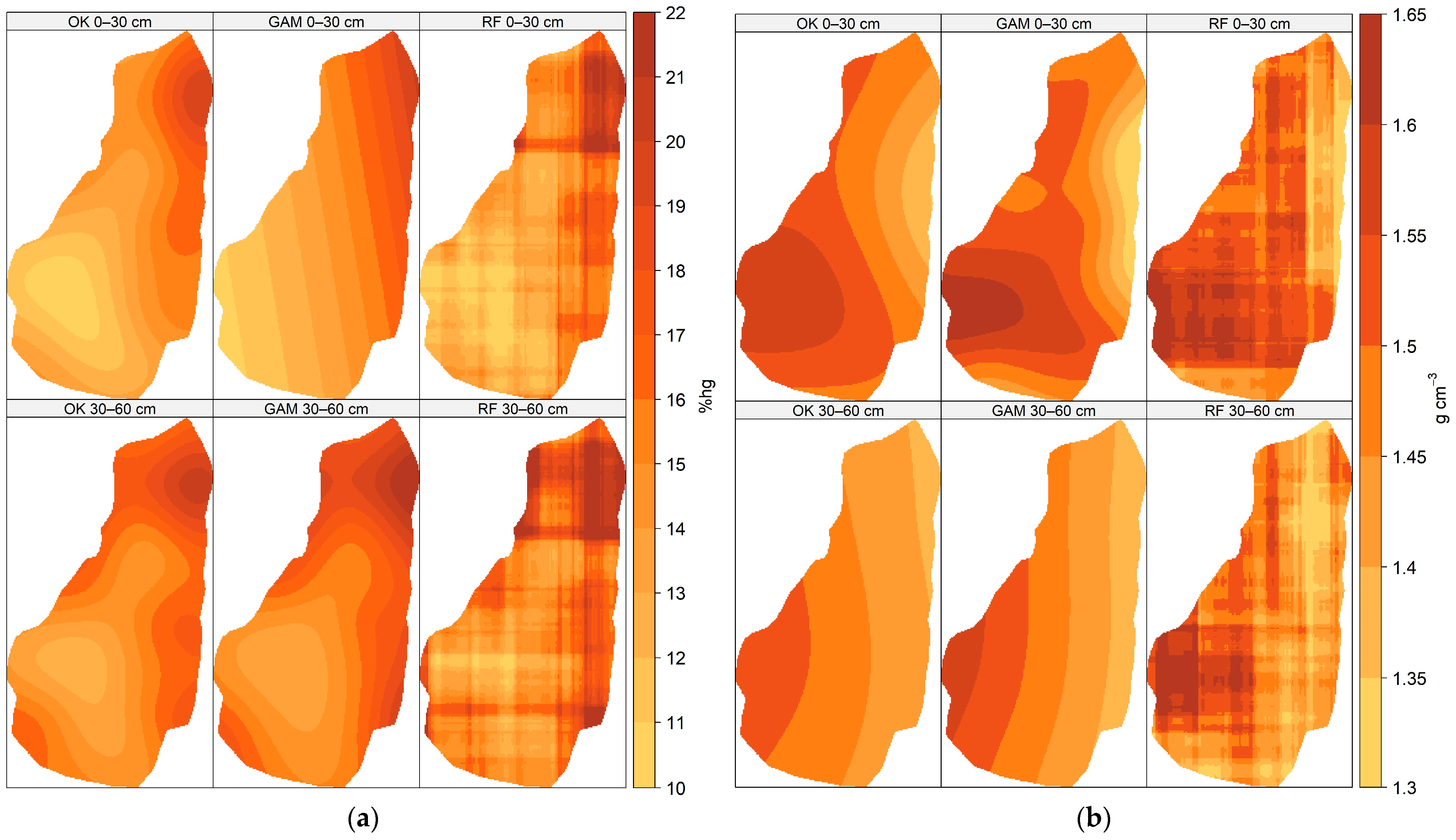
The maps for the other variables are included in Appendix C for detailed consultation. This methodological visual comparison strategy has been widely adopted in digital soil mapping studies, as it allows us to validate both the accuracy and the practical applicability of the models used [40].
3.7. Prediction and Mapping
3.7.1. Texture
For the construction of the soil texture map (Figure 7), the predictions of % sand and % clay were combined with OK’s predictions of % silt to achieve a more precise classification using the Soil Survey Staff textural triangle [126], which is essential for agricultural zoning and precision agriculture. This approach is supported by studies such as those of Ballabio et al. [127] and Padarian et al. [128], which reported high accuracy in texture maps constructed using RF.
Figure 7.
Soil texture map at both depths.
In addition, the OK method has proven effective at predicting continuous variables such as % silt and provides a more coherent spatial structure [129]. The predominant textural class was sandy clay loam, with coverages of 70.3% (0–30 cm) and 56.6% (30–60 cm); followed by clay loam with 24.64% and 32.12%; and clay with 2.9% and 10.4%, respectively. The soil texture map facilitates the identification of homogeneous areas, enabling differentiated irrigation strategies based on terrain characteristics.
Since texture directly influences moisture retention capacity and infiltration rate, soils with a higher proportion of sand require more frequent watering and shallower irrigation depths. In contrast, clay soils retain more water but have lower infiltration rates. This information is essential for selecting crops suited to specific textural conditions and contributes to a more precise, efficient, and sustainable agriculture.
3.7.2. KS
The predictions generated for OM, % sand, % clay, and BD (Table 2 and Figure 8) provided a spatial reference of KS for the entire ID 001. Despite being based on estimates rather than direct measurements, these values indicate that approximately 23.45% of the total district area has a KS of less than 4.00 mm h−1 in the surface layer (0–30 cm). This percentage increases significantly to 50.59% in the subsurface layer (30–60 cm).
Table 2.
Percentage distribution of soil infiltration.
Figure 8.
Soil infiltration map at both depths.
It is worth noting that the map should be considered a reference rather than a diagnostic tool, as it depends on the quality of laboratory data and model assumptions. Nonetheless, it is useful for irrigation planning and for identifying areas prone to waterlogging, in line with indirect methodologies applied in other studies. In addition, it facilitates more focused and efficient field sampling campaigns, as suggested by studies that have used indirect methodologies to estimate infiltration in the absence of in situ measurements [130,131].
3.8. Integration of Soil Variables into Decision Support System
The spatial modeling process produced vector layers (shapefiles) generated by depth (0–30 cm and 30–60 cm) from the spatial R predictions of soil physicochemical properties, which were later integrated into the Geographic Information System (GIS). These layers contain plot-weighted soil values within ID 001, providing a detailed, localized characterization of soil physical and nutritional status.
This allows for the integration of information on soil physicochemical properties, climatological data, irrigation infrastructure, and other elements necessary for irrigation management into an open-source DSS that democratizes access to precision agriculture tools and bridges the gap between environmental modeling and its practical and actual agronomic application (Figure 9). This approach would reduce the cost of commercial platforms and eliminate a critical economic barrier for districts and irrigation units.
Figure 9.
Conceptual architecture of decision support system.
The proposed DSS will transform irrigation management by incorporating specific findings on FC, PWP, and KS. In areas with limited drainage (KS < 4 mm h−1), the system will recommend reduced depths and increased frequencies to prevent waterlogging.
Zhang et al. [132] report that DSSs, when based on local evidence, can improve water-use efficiency by 20–30%. The integration of these components into a unified, accessible, and low-cost platform represents a significant step toward more resilient and sustainable agriculture in the ID 001, aligning with the digitization of the agricultural sector and prioritizing affordability and local relevance [133].
The integration of DSS with GIS is a well-established strategy across multiple investigations addressing precision agriculture, given its ability to improve input use efficiency, increase productivity, and mitigate environmental impacts [134,135,136]. This approach is especially relevant in contexts involving technified irrigation, as spatially detailed information enables precise adjustment of fertilization rates and water management according to the particular soil conditions of each plot [137,138].
The Civil Association of Users (ACU, in Spanish) of ID 001 currently uses the plot-weighted results generated in this research to provide feedback to the “Kilimo” irrigation management web platform [139] from the company ClimateTech, which allows each plot to be monitored and recommendations to be received on the irrigation rates to be applied during the crop cycle. This service costs USD 20 ha−1.
Data integration enables Kilimo’s recommendations to be based on local data, significantly improving their accuracy compared to generic estimates. If water-saving targets are met at the end of the cycle, the company gives them a $30 ha−1 bonus. Antle et al. [140] point out that this “data as a service” approach is the emerging standard in digital agriculture, where data quality and location directly determine the usefulness of recommendations.
4. Discussion
The results of this study reveal the spatial and vertical complexity of soil physicochemical properties in ID 001, with direct implications for precision agricultural management. Comparative analysis of predictive models revealed clear differences among the evaluated approaches, highlighting complementary strengths of geostatistical and machine learning methods.
The RF model showed superior performance in predicting soil chemical properties, such as nitrogen forms, available phosphorus, and macronutrients, thanks to its ability to model nonlinear relationships and complex interactions between soil variables. This behavior is consistent with studies conducted in semi-arid regions, where spatial heterogeneity of the soil reduces the effectiveness of traditional linear methods and where machine learning algorithms have proven more robust at capturing complex soil patterns [141,142].
In contrast, the OK method showed greater accuracy in estimating physical soil properties, such as texture and bulk density, where spatial autocorrelation was stronger (MI = 0.19–0.35) and more stable. This pattern is consistent with that reported by Ballabio et al. [127], who observed that physical properties maintain persistent spatial structures at the continental scale, supporting the use of geostatistical techniques for their modeling.
GAMs performed worst, likely due to their sensitivity to data smoothing assumptions in the presence of high local variability. In several cases, R2 values were negative, suggesting that this approach is not suitable for data with strong residual autocorrelation or extreme deviations from normality (skewness up to 8.24; kurtosis up to 78.61). This limitation underscores the importance of selecting algorithms that align with the structure of soil data, especially for properties with high variability, such as Na+ and AP [39].
From an edaphic perspective, the negative correlations between pH and micronutrient availability (Fe2+, r = −0.65; Mn2+, r = −0.78) confirm that alkalinity (pH ≈ 8.0) acts as a limiting factor for the bioavailability of essential nutrients. At the same time, EC reflects the accumulation of soluble ions, with positive correlations with Ca2+ (r = 0.52) and K+ (r = 0.45), evidencing differential leaching and redistribution of salts in the soil profile.
This pattern coincides with that reported by Shrivastava and Kumar [143], who note that salinity and alkalinity reduce the solubility and absorption of micronutrients (Fe2+, Mn2+, Zn2+, AP, K+) by altering the ionic balance and soil structure, affecting plant productivity. Complementarily, Qadir et al. [77] document that the accumulation of salts and sodium in irrigated soils in arid and semi-arid areas causes physical and chemical degradation, limiting permeability, water flow, and nutrient availability, with significant economic and environmental impacts.
The FC and PWP values, combined with the predominant sandy loam texture, indicate a usable water reserve of approximately 9.7%, suitable for extensive crops under efficient irrigation. However, it may be limiting under conditions of water stress or high evaporative demand, especially in areas with saturated hydraulic conductivity (KS) below 4 mm h−1. This behavior is consistent with that reported by Fu et al. [144] and Kim et al. [145], who demonstrated that irrigation water salinity and Na+ accumulation reduce infiltration and water availability, thereby decreasing irrigation efficiency and promoting salt accumulation in the soil profile in irrigated soils in arid and semi-arid regions.
The extreme variability of exchangeable sodium (Na+)—with coefficients of variation exceeding 200%—poses a critical agronomic challenge, as it induces clay dispersion, reduces infiltration, and deteriorates soil structure. These effects are associated with secondary sodification processes, common in arid areas irrigated with groundwater or mixtures of varying quality, where high evapotranspiration and low leaching favor the accumulation of salts in the profile [146,147]. In this regard, management must be based on accurate spatial diagnoses of salinity to enable the application of remediation and efficient water use strategies [148], including calcium amendments, salinity-tolerant crops, and localized irrigation to restore soil structure and prevent degradation.
Finally, some limitations must be acknowledged. The unbalanced sample design, with only four natural vegetation sites compared to 97 agricultural sites, limits the statistical capacity to detect significant differences between land uses, as evidenced by the non-significant PERMANOVA analysis (ρ = 0.161). Furthermore, the sampling depth (0–60 cm) does not capture processes in deeper horizons, which are relevant for crops with extensive root systems.
Future research should incorporate more balanced designs and complementary variables, such as biological properties or active carbon indicators, and greater depths to capture leaching dynamics, as well as remote predictor variables (multispectral images, LiDAR) to improve the accuracy of digital mapping models. It is also recommended to implement multitemporal monitoring and biological parameters, linking edaphic variability to productivity and environmental quality, thereby strengthening the practical application of predictive models for more accurate and sustainable agricultural management.
The prediction maps generated using OK and RF are an essential tool for decision-making in precision agriculture, as they enable the identification of areas with specific limitations in terms of fertility, salinity, or infiltration. Their integration into DSSs can optimize irrigation scheduling, differentiated fertilizer application, and crop selection according to local soil suitability. These cartographic products provide a solid technical basis for implementing sustainable water and soil management policies in semi-arid regions, in line with the principles of agricultural sustainability and resilience promoted by the FAO and the 2030 Agenda and with the role of DSM and DSSs described by Arrouays et al. [149] and Lo Papa et al. [150].
5. Conclusions
The results of this study confirm the high spatial and vertical complexity of soil physical–chemical properties in Irrigation District 001 (ID 001), revealing marked edaphic heterogeneity that conditions the efficiency of irrigation and fertilization in semi-arid irrigated agricultural systems. The high spatial variability of available phosphorus, exchangeable sodium (Na+), and electrical conductivity (EC), together with the significant vertical stratification of organic matter, total nitrogen, and total carbon, reflects the interaction between agricultural management practices and site-inherent soil processes.
Alkaline pH (≈8.0) and EC are identified as key regulatory variables of nutrient availability, defining edaphic gradients relevant to agricultural planning. In this context, well-defined chemical relationships were observed, where pH controls the bioavailability of micronutrients (negative correlations with Fe2+ and Mn2+), while EC reflects salt leaching and redistribution processes (positive correlations with Ca2+ and K+). Likewise, spatial autocorrelation reduced the effective sample size by 30–70%, thereby affecting statistical power and underscoring the need for explicit spatial approaches.
From a predictive standpoint, Random Forest (RF) showed the best performance for most chemical properties, while Ordinary Kriging (OK) proved more effective for physical properties with a well-defined spatial structure. The combination of both methods is established as a robust and complementary strategy to improve the accuracy of Digital Soil Mapping (DSM) in edaphically complex environments with high variability.
The main contribution of this work lies in proposing an integrated methodological framework that combines classical statistics, geostatistics, and machine learning for the characterization of heterogeneous agricultural soils; evaluating the strengths and limitations of predictive models under non-normal conditions and high variability; and facilitating the transfer of scientific knowledge into practice by generating spatial products ready for integration into digital agricultural management platforms.
RF and OK-derived maps are key technical tools for agricultural zoning, irrigation scheduling, and the design of differentiated fertilization schemes, as they enable the identification of areas with specific infiltration or salinity limitations. These products provide a solid foundation for sustainable water and soil management, strengthening precision agriculture and the resilience of agroecosystems.
In the future, research will focus on developing a low-cost, open-source Decision Support System (DSS) that integrates predictive models calibrated with remote sensors, meteorological data, and the ID 001 irrigation infrastructure. This approach seeks to democratize access to precision agriculture tools, reduce economic barriers (around $20 USD ha−1 on commercial platforms), and empower farmers with scientific information that optimizes profitability, resource efficiency, and environmental sustainability.
Overall, the results highlight the potential of DSM, supported by statistical and machine learning models, as an effective strategy for optimizing water and nutrient resources, improving agronomic planning, and promoting more sustainable agricultural systems in the face of the challenges posed by climate change and soil degradation.
Author Contributions
Conceptualization, O.G.-C. and M.A.B.-G.; methodology, M.A.B.-G., O.G.-C., J.V.P.-H. and J.A.U.-V.; software, O.G.-C. and M.A.B.-G.; validation, M.A.B.-G. and O.G.-C.; formal analysis, M.A.B.-G. and O.G.-C.; investigation, O.G.-C., M.A.B.-G., A.A.E.-G., A.L.-P., J.V.P.-H. and J.A.U.-V.; resources, M.A.B.-G.; data curation, O.G.-C. and M.A.B.-G.; writing—original draft preparation, O.G.-C. and M.A.B.-G.; writing—review and editing, O.G.-C., M.A.B.-G., A.A.E.-G., A.L.-P., J.V.P.-H. and J.A.U.-V.; visualization, O.G.-C. and M.A.B.-G. All authors have read and agreed to the published version of the manuscript.
Funding
This study was financed by the Consejo Nacional de Humanidades, Ciencias y Tecnologías (CONAHCYT) for funding the Ph.D. studies of O.G.-C. (Scholarship no. 789301).
Data Availability Statement
The original contributions presented in the study are included in the article, further inquiries can be directed to the corresponding author.
Acknowledgments
The authors wish to thank the CONAHCYT, as well as the Hydrosciences Postgraduate Course of the Colegio de Postgraduados, for the support provided in the development of this research study. Asociación de Usuarios Junta de Aguas del Distrito de Riego 001 Asociación Civil (administration period 2021–2023) and to the National Water Commission (CONAGUA, in Spanish), Irrigation District 001 Office in Pabellón de Arteaga, Aguascalientes Local Directorate, for their valuable support and collaboration during the fieldwork phase. Claudia Hidalgo Moreno, from the Soil Fertility and Environmental Chemistry Laboratory, and Víctor Manuel Ordaz Chaparro, from the Soil Physics Laboratory, for their support in the processing of soil samples. María Elena Sánchez-Salazar translated the manuscript into English.
Conflicts of Interest
The authors declare no conflicts of interest.
Appendix A
This appendix presents the mathematical formulations of the statistical and geostatistical methods used to model and map soil physical and chemical properties in Irrigation District 001, Aguascalientes, Mexico.
Appendix A.1. Box–Cox Transformation
It was applied to stabilize variance and approach normality:
where represents the original value and is the transformation parameter.
Appendix A.2. Geostatistical Interpolation (Ordinary Kriging)
Spatial prediction was performed using ordinary kriging:
where is the estimated value at the unsampled point; is the measured value; is the weight assigned to the observed value; and n is the number of points sampled.
The value of the weights (Equation (A3)) is obtained by minimizing the variance of the estimation error (Kriging’s variance), which results in a system of equations, also known as the Lagrange system.
where is the semi-variance function (semivariogram) for a distance h; and µ is the Lagrange multiplier associated with the constraint that the sum of weights is 1.
Appendix A.3. Generalized Additive Models (GAM)
Nonlinear relationships between soil properties and environmental covariates were modeled using GAM:
where Y is the response variable; is the expected value of the response; g is the binding function (e.g., Normal, LogNormal, and others); is the intercept; are smooth functions (splines, local regression, among others) applied to the predictor variables; and p is the number of predictors.
Appendix A.4. Random Forest
Machine learning-based regression using Random Forests was applied to capture nonlinear interactions among soil-forming factors. From a set of training data , the algorithm does the following:
Random B subsets are generated using Bootstrap sampling with replacement of the original dataset. Then, for each Db subset, a Tb decision tree is constructed using a random selection of a subset of features at each node to divide. Finally, the classification of the trees is carried out by majority vote of the trees (Equation (A5)), and a regression is performed using the average of the predictions (Equation (A6)):
Appendix A.5. Spatial Autocorrelation Analysis (Moran’s I and SAR Models)
Spatial dependence was evaluated using Moran’s I statistic (, MI) and Spatial Autoregressive Regression (SAR, ) models:
where is the number of cases (polygons or points), is the mean of the variable, is the value of the variable X in site i, is the value of the variable X in site j, and is the weighting associated with site i relative to site j.
where the georeferenced variable has a normal or quasi-normal distribution, n is the sample size, n* is the calculated effective sample size, and ρ is the spatial autocorrelation parameter.
Appendix B
This appendix presents the complementary statistical results supporting the analyses discussed in the main manuscript. The tables included provide descriptive statistics, analysis of variance, correlation analyses between soil salinity and acidity indicators, spatial autocorrelation indices, and comparative performance metrics of the applied prediction models.
Table A1.
Measures of central tendency, variability, shape, and normality.
Table A2.
Analysis of Variance (ANOVA).
Table A3.
Spearman correlations between pH, EC, and chemical variables.
Table A4.
Moran’s I and sample size.
Table A5.
Comparison of errors between interpolation/prediction methods.
Appendix C
Figure A1.
Comparative predictions using OK, GAM, and RF. (a) EC; (b) TC.
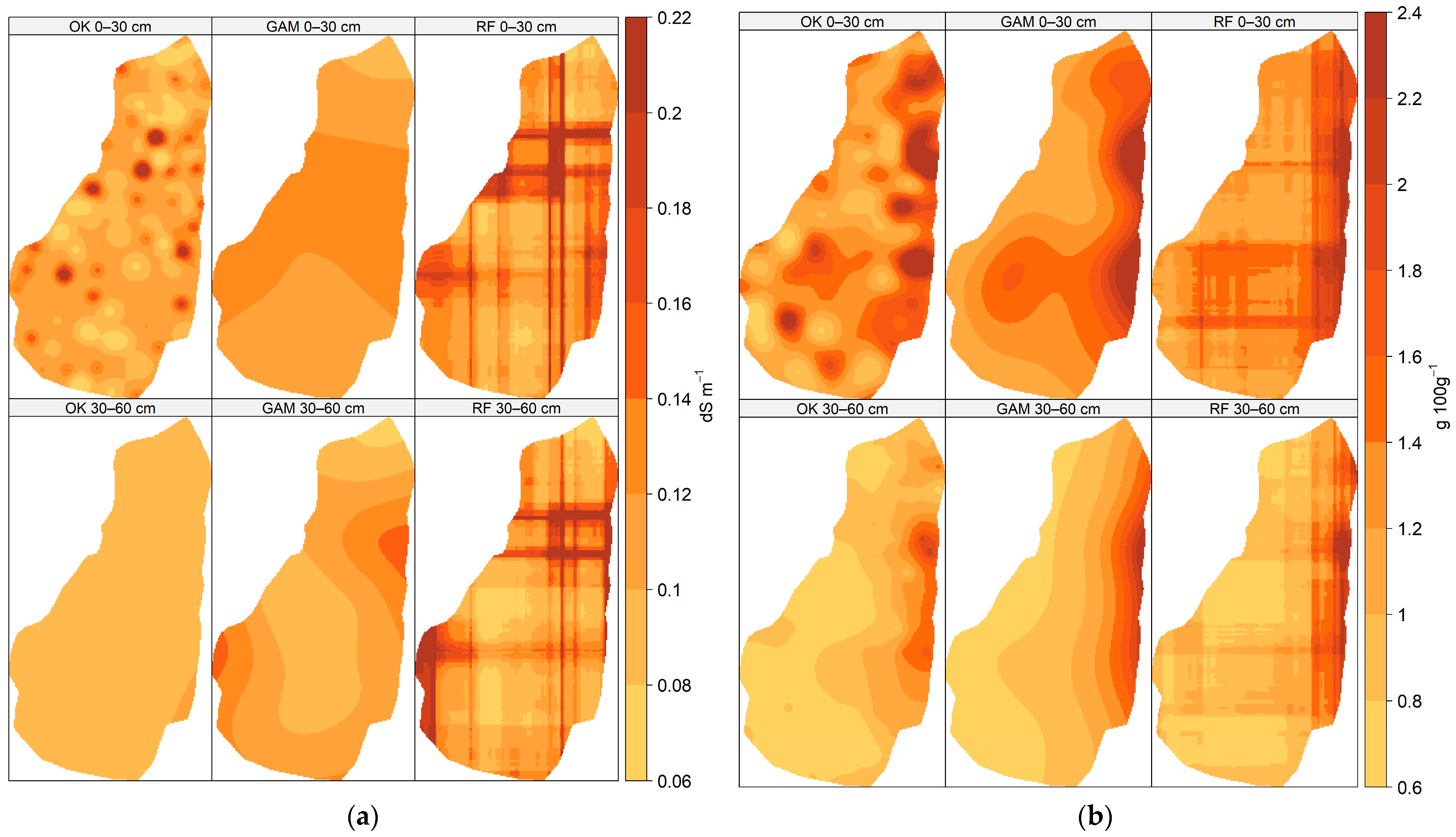
Figure A2.
Comparative predictions using OK, GAM, and RF. (a) TN; (b) AP.
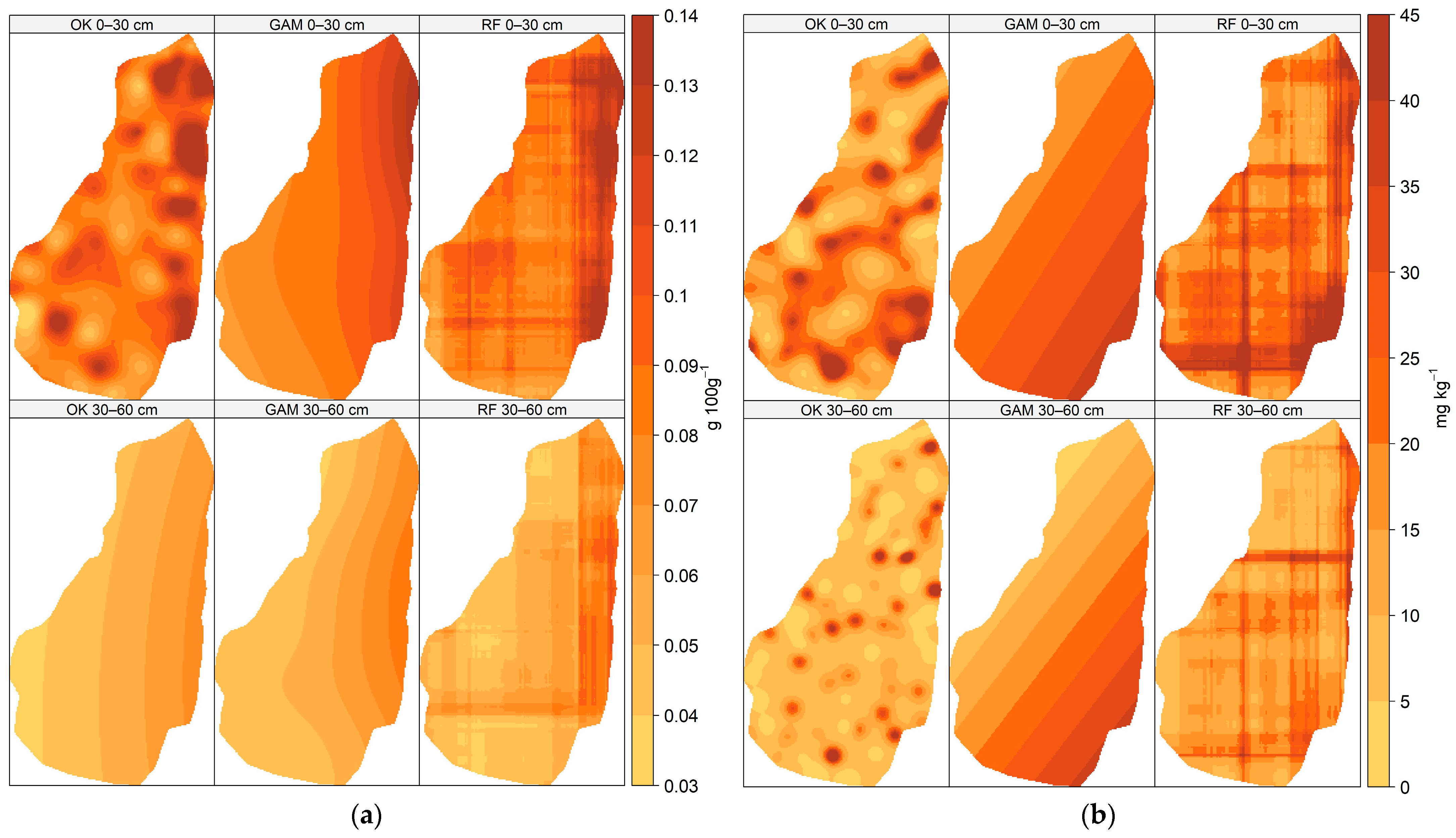
Figure A3.
Comparative predictions using OK, GAM, and RF. (a) K+; (b) Ca2+.
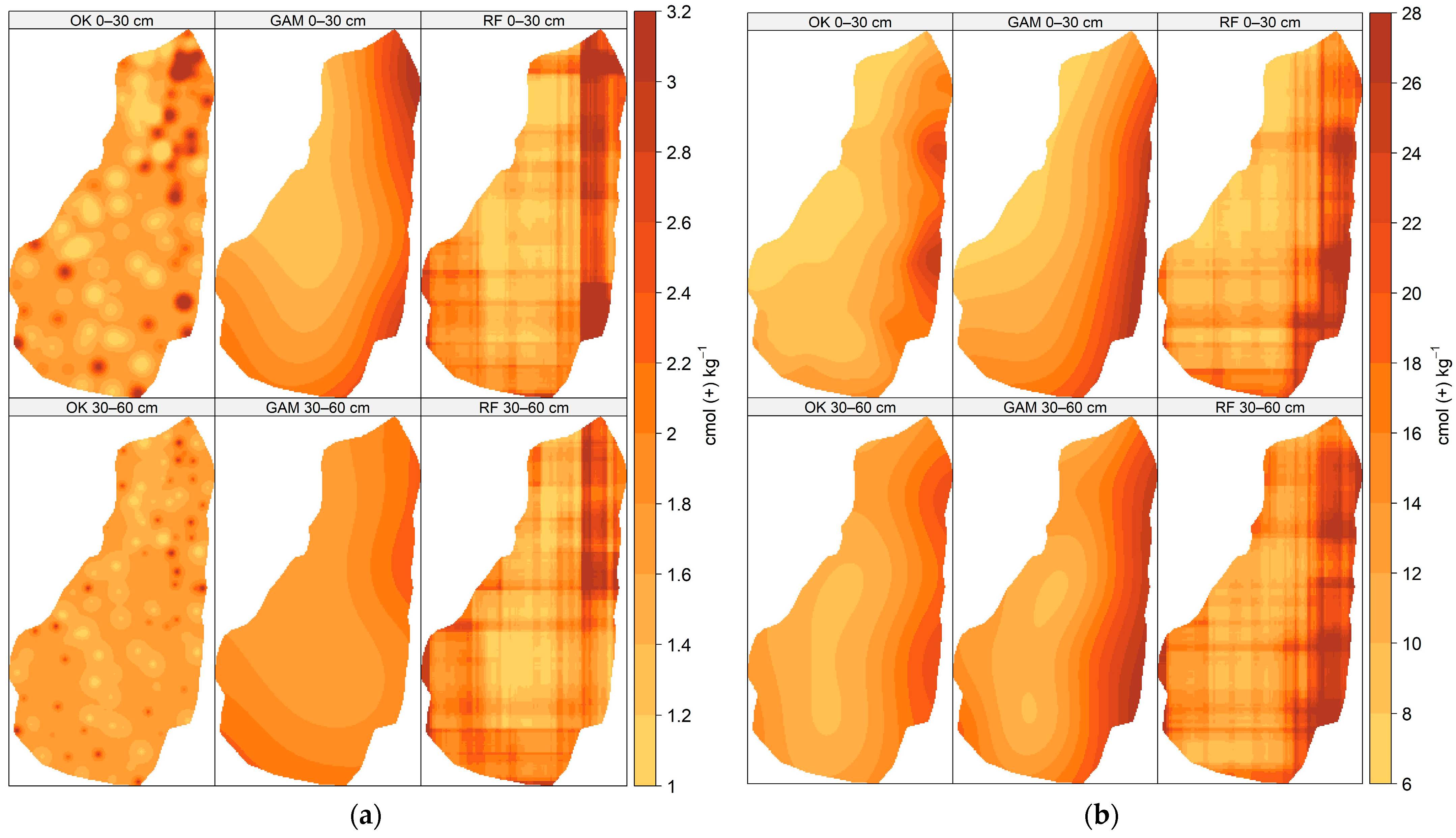
Figure A4.
Comparative predictions using OK, GAM, and RF. (a) Mg2+; (b) Na+.
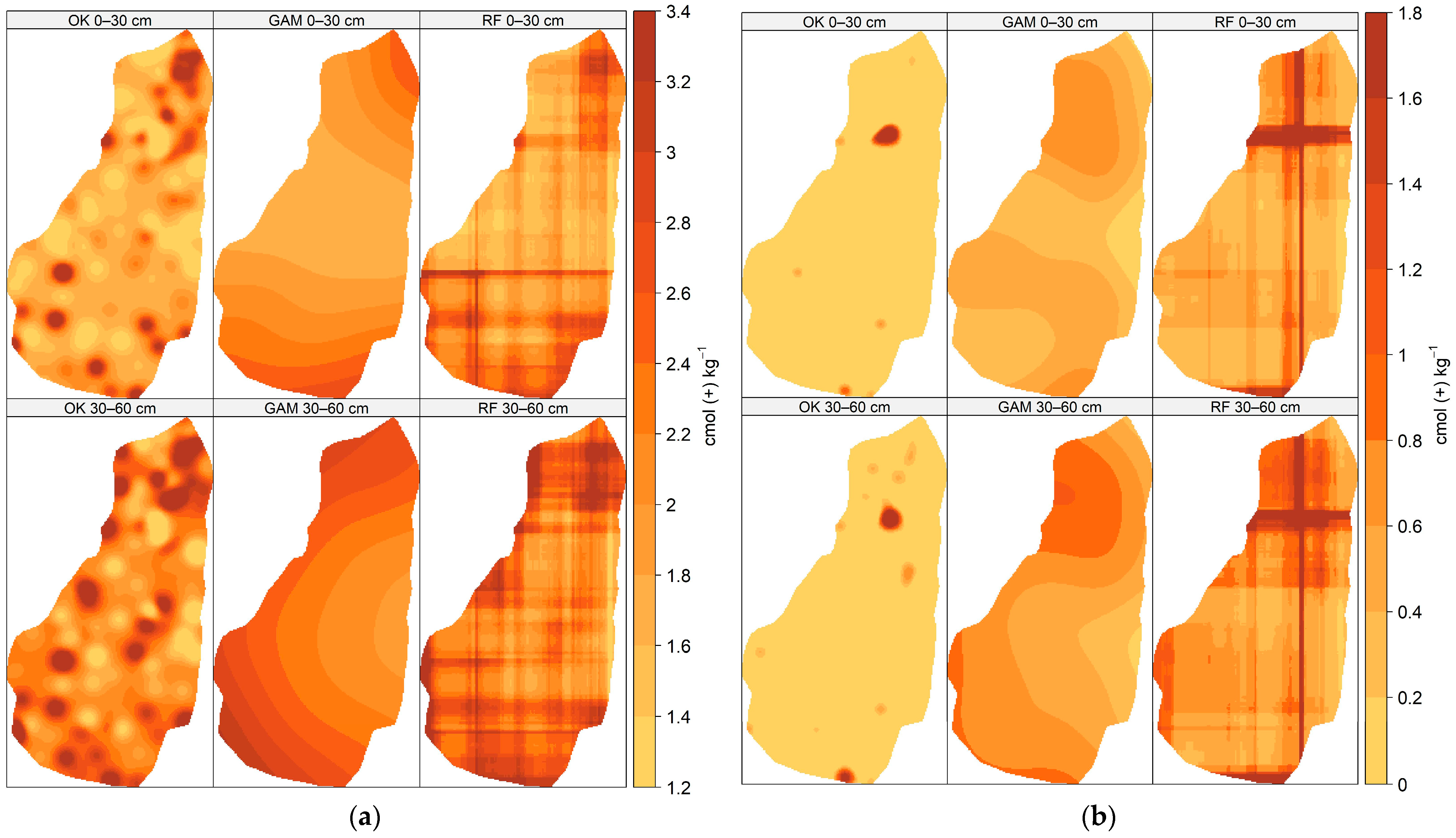
Figure A5.
Comparative predictions using OK, GAM, and RF. (a) NO3−–N; (b) NH4+–N.
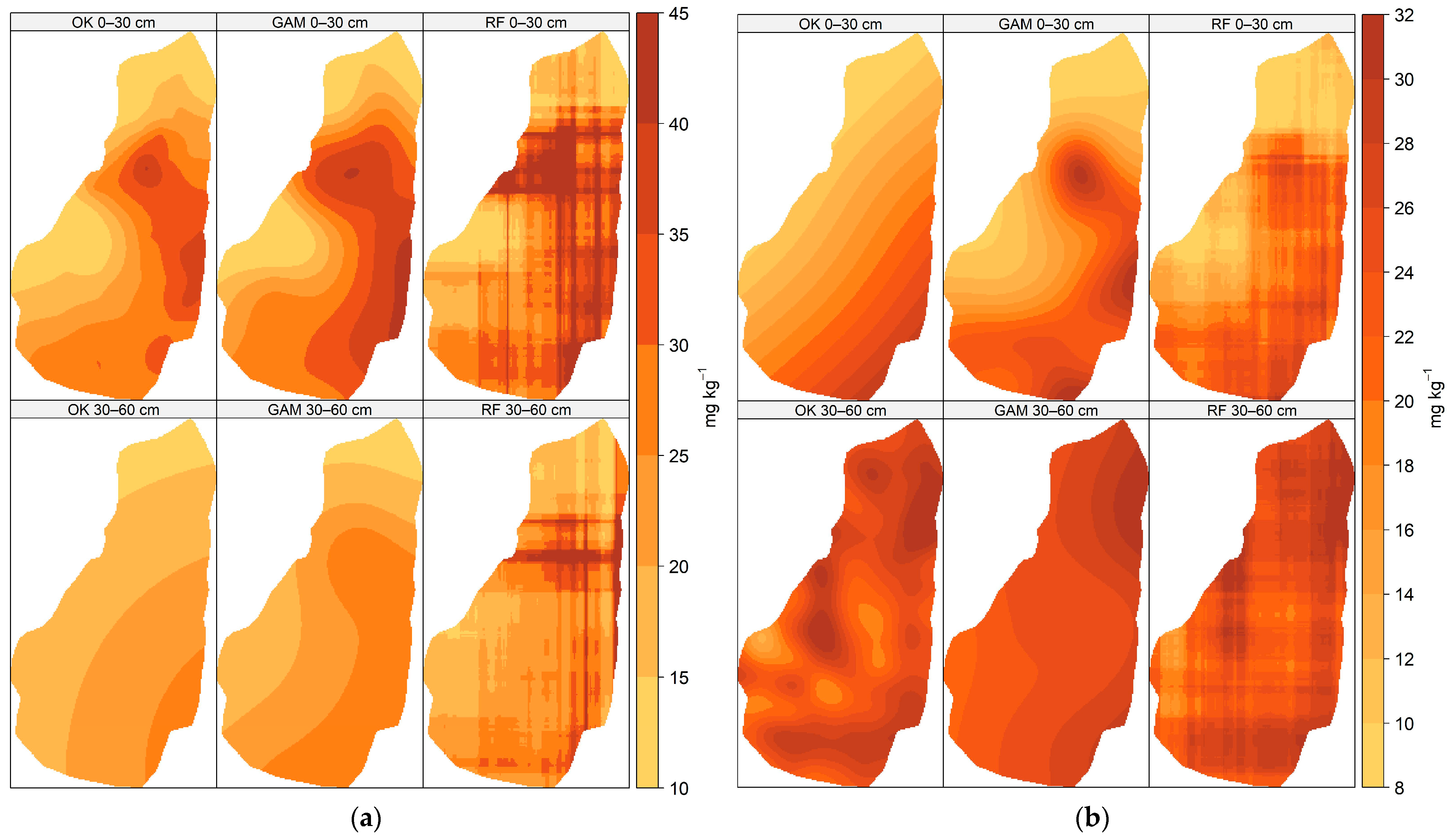
Figure A6.
Comparative predictions using OK, GAM, and RF. (a) Fe2+; (b) Cu2+.
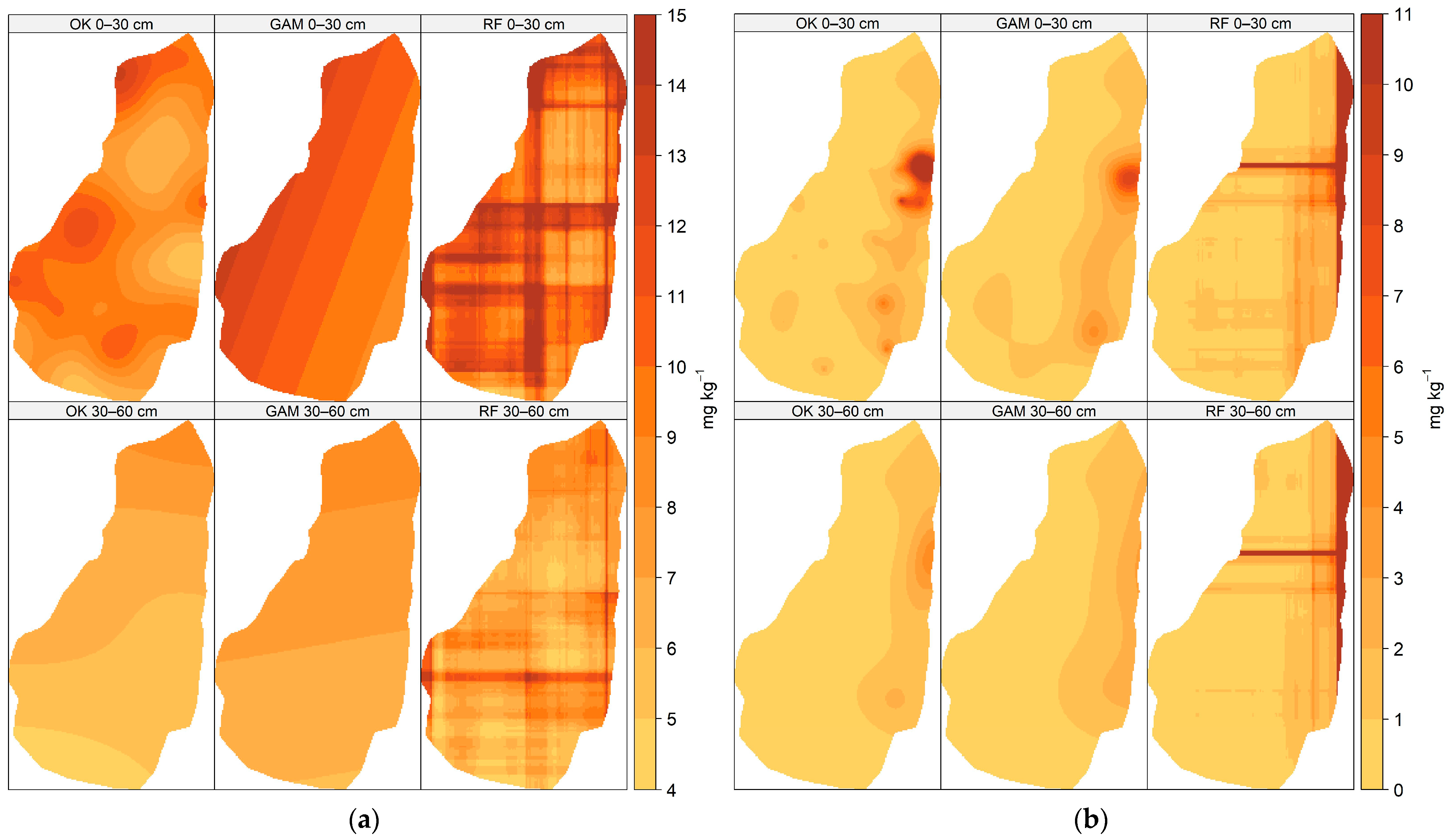
Figure A7.
Comparative predictions using OK, GAM, and RF. (a) Zn2+; (b) Mn2+.
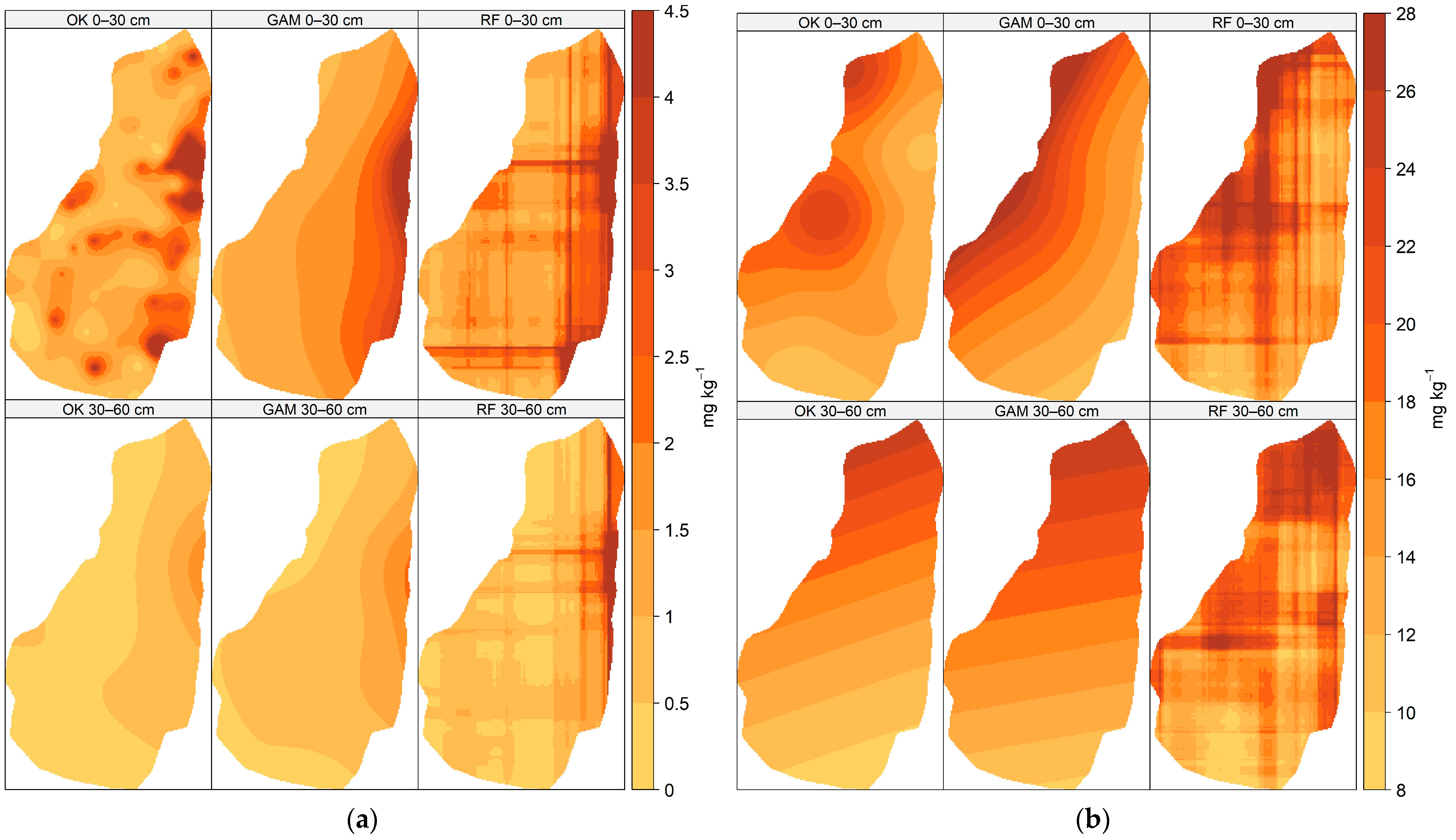
Figure A8.
Comparative predictions using OK, GAM, and RF. (a) % sand; (b) % silt.
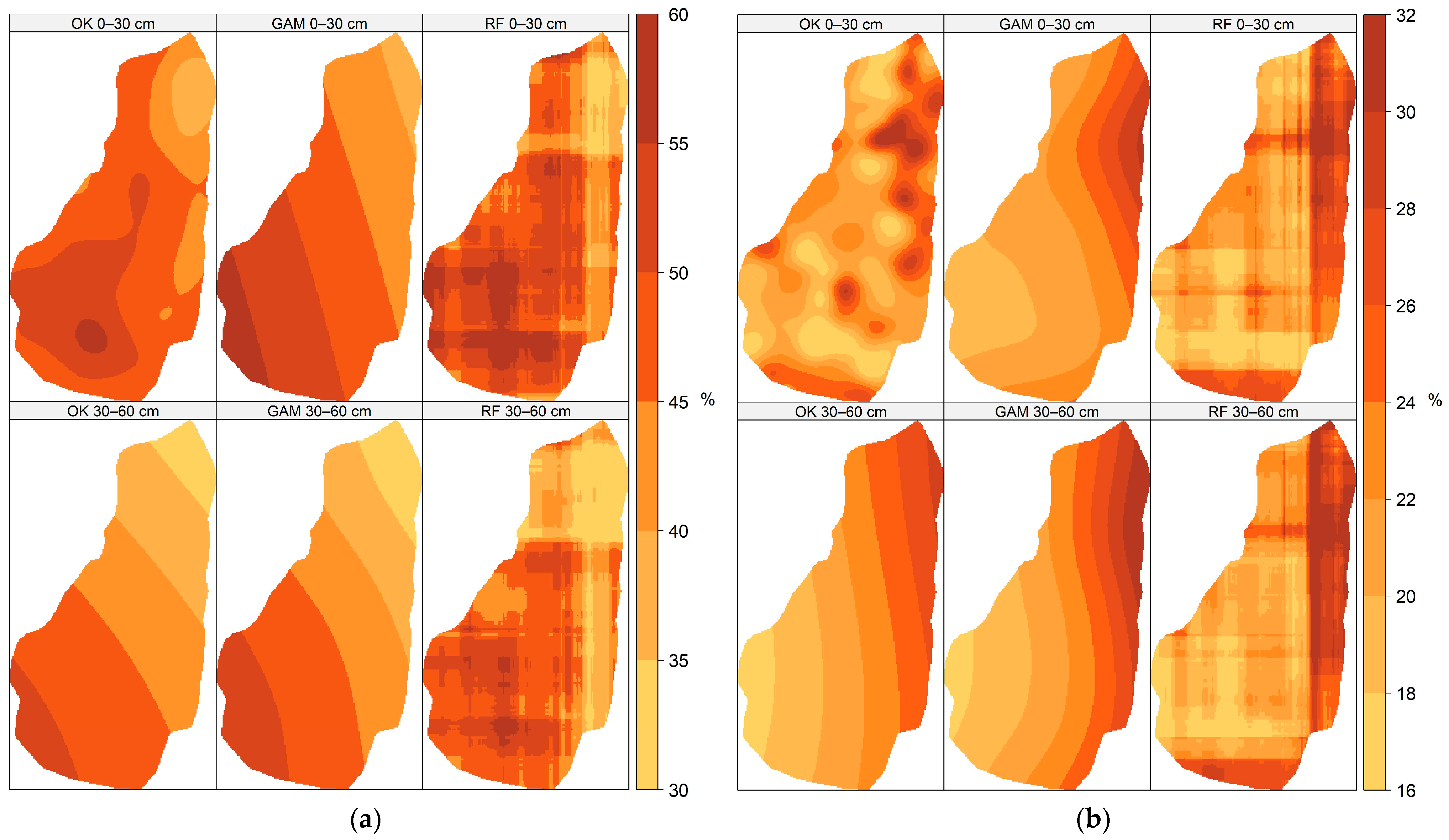
Figure A9.
Comparative predictions using OK, GAM, and RF. (a) % clay; (b) FC.
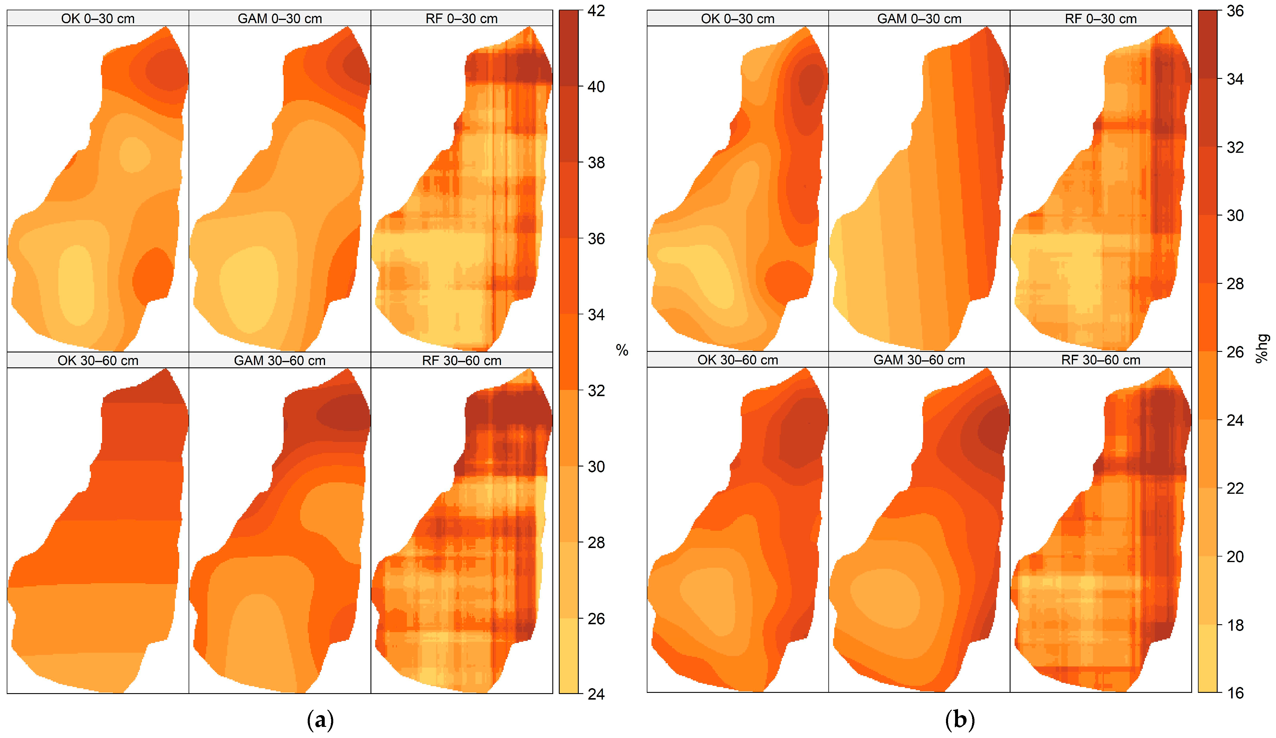
Figure A10.
Comparative predictions using OK, GAM, and RF. (a) PWP; (b) BD.
References
- Spring, Ú.O.; Cohen, I.S. Water Resources in Mexico: A Conceptual Introduction. In Water Resources in Mexico: Scarcity, Degradation, Stress, Conflicts, Management, and Policy; Oswald Spring, Ú., Ed.; Springer: Berlin/Heidelberg, Germany, 2011; pp. 3–17. ISBN 978-3-642-05432-7. [Google Scholar]
- Vélez, E.P.; Saez, E.M. Water Use for Agriculture in Mexico. In Water Resources in Mexico: Scarcity, Degradation, Stress, Conflicts, Management, and Policy; Oswald Spring, Ú., Ed.; Springer: Berlin/Heidelberg, Germany, 2011; pp. 129–143. ISBN 978-3-642-05432-7. [Google Scholar]
- Rockström, J.; Williams, J.; Daily, G.; Noble, A.; Matthews, N.; Gordon, L.; Wetterstrand, H.; DeClerck, F.; Shah, M.; Steduto, P.; et al. Sustainable Intensification of Agriculture for Human Prosperity and Global Sustainability. Ambio 2017, 46, 4–17. [Google Scholar] [CrossRef] [Scilit]
- Ortuani, B.; Chiaradia, E.A.; Priori, S.; L’Abate, G.; Canone, D.; Comunian, A.; Giudici, M.; Mele, M.; Facchi, A. Mapping Soil Water Capacity Through EMI Survey to Delineate Site-Specific Management Units Within an Irrigated Field. Soil Sci. 2016, 181, 252. [Google Scholar] [CrossRef] [Scilit]
- Santiago-Mejía, B.E.; Martínez-Menez, M.R.; Rubio-Granados, E.; Vaquera-Huerta, H.; Sánchez-Escudero, J. Variabilidad espacial de propiedades físicas y químicas del suelo en un sistema lama-bordo en la Mixteca Alta de Oaxaca, México. Agric. Soc. Desarro. 2018, 15, 275–288. [Google Scholar] [CrossRef] [Scilit]
- Vega-Blancas, V.d.J.; Fernández-Reynoso, D.S.; Macedo-Cruz, A.; Rios-Berber, J.D.; Ruiz-Bello, A. Análisis de la fertilidad del suelo mediante la validación e interpolación Kriging de sus variables. Rev. Terra Latinoam. 2022, 40, e1573. [Google Scholar] [CrossRef] [Scilit]
- Moreno, V.M.R.; Corral, J.A.R.; Ramírez, J.S.P.; Serna, M.M.S. Mapeo espacial de la salinidad del suelo a través de sensores remotos. Estudio de caso norte de Tamaulipas. Rev. Mex. Cienc. Agríc. 2017, 7, 2577–2587. [Google Scholar] [CrossRef] [Scilit]
- Pérez-Rodríguez, G.; López-Santos, A.; Velásquez-Valle, M.A.; Villanueva-Díaz, J.; García-Rodríguez, J.L. Spatial Distribution of Soil Organic Carbon by Digital Mapping: The Case of the Medio Aguanaval River Sub-Basin. Ing. Agríc. Biosist. 2021, 13, 227–245. [Google Scholar] [CrossRef] [Scilit]
- Guevara, M.; Vargas, R. Predicción de carbono orgánico en los suelos de México a 1 m de profundidad y 90 m de resolución espacial (1999–2009). Rev. Terra Latinoam. 2021, 39, e1241. [Google Scholar] [CrossRef] [Scilit]
- Estrada-Godoy, F.; Cruz-Cárdenas, G.; Ochoa-Estrada, S.; Silva, J.T. Cartografía digital de suelos con regresión-Kriging y datos de sensores remotos. Rev. Terra Latinoam. 2023, 41, e1617. [Google Scholar] [CrossRef] [Scilit]
- Fusaro, C.; Sarria-Guzmán, Y.; González-Jiménez, F.E.; Saba, M.; Coronado-Hernández, O.E.; Castrillón-Ortíz, C. Modelling the Spatial Distribution of Soil Organic Carbon Using Machine Learning and Remote Sensing in Nevado de Toluca, Mexico. Geomatics 2025, 5, 43. [Google Scholar] [CrossRef] [Scilit]
- Sharma, P.; Shukla, M.K.; Mexal, J.G. Spatial Variability of Soil Properties in Agricultural Fields of Southern New Mexico. Soil Sci. 2011, 176, 288. [Google Scholar] [CrossRef] [Scilit]
- Krasilnikov, P.; Gutiérrez-Castorena, M.d.C.; Ahrens, R.J.; Cruz-Gaistardo, C.O.; Sedov, S.; Solleiro-Rebolledo, E. Soil Research and Soil Mapping History. In The Soils of Mexico; Krasilnikov, P., Gutiérrez-Castorena, M.d.C., Ahrens, R.J., Cruz-Gaistardo, C.O., Sedov, S., Solleiro-Rebolledo, E., Eds.; Springer: Dordrecht, The Netherlands, 2013; pp. 5–23. ISBN 978-94-007-5660-1. [Google Scholar]
- Qiu, J.; Liu, F.; Wang, D.; Yan, K.; Guo, J.; Huang, W.; Feng, Y. Mapping Key Soil Properties in Low Relief Areas Using Integrated Machine Learning and Geostatistics. Ecol. Indic. 2025, 171, 113228. [Google Scholar] [CrossRef] [Scilit]
- Sridevy, S.; Raj, M.N.; Kumaresan, P.; Balakrishnan, N.; Tilak, M.; Raj, J.A.S.; Rani, P.J.I. Mapping of Soil Properties Using Machine Learning Techniques. Int. J. Environ. Clim. Change 2023, 13, 684–700. [Google Scholar] [CrossRef] [Scilit]
- Farooq, I.; Bangroo, S.A.; Bashir, O.; Shah, T.I.; Malik, A.A.; Iqbal, A.M.; Mahdi, S.S.; Wani, O.A.; Nazir, N.; Biswas, A. Comparison of Random Forest and Kriging Models for Soil Organic Carbon Mapping in the Himalayan Region of Kashmir. Land 2022, 11, 2180. [Google Scholar] [CrossRef] [Scilit]
- Han, H.; Suh, J. Spatial Prediction of Soil Contaminants Using a Hybrid Random Forest–Ordinary Kriging Model. Appl. Sci. 2024, 14, 1666. [Google Scholar] [CrossRef] [Scilit]
- INEGI. Conjunto de Datos Vectorial Edafológico. Escala 1:250 000 Serie II Continuo Nacional Zacatecas; INEGI: Aguascalientes, Mexico, 2007. [Google Scholar]
- SEMARNAT NORMA Oficial Mexicana NOM-021-RECNAT-2000, Que Establece Las Especificaciones de Fertilidad, Salinidad y Clasificación de Suelos. Estudios, Muestreo y Análisis. Available online: https://www.dof.gob.mx/nota_detalle.php?codigo=717582&fecha=31/12/2002#gsc.tab=0 (accessed on 28 June 2025).
- Olsen, S.R.; Cole, C.V.; Watanabe, F.S.; Dean, L.A. Estimation of Available Phosphorus in Soils by Extraction with Sodium Bicarbonate; USDA Circular; United States Department of Agriculture (USDA): Washington, DC, USA, 1954.
- Walkley, A.; Black, I.A. An Examination of the Degtjareff Method for Determining Soil Organic Matter, and a Proposed Modification of the Chromic Acid Titration Method. Soil Sci. 1934, 37, 29–38. [Google Scholar] [CrossRef] [Scilit]
- Lindsay, W.L.; Norvell, W.A. Development of a DTPA Soil Test for Zinc, Iron, Manganese, and Copper. Soil Sci. Soc. Am. J. 1978, 42, 421–428. [Google Scholar] [CrossRef] [Scilit]
- Bower, C.A.; Reitemeier, R.F.; Fireman, M. Exchangeable Cation Analysis of Saline and Alkali Soils. Soil Sci. 1952, 73, 251–262. [Google Scholar] [CrossRef] [Scilit]
- U.S. Salinity Laboratory Staff. Diagnosis and Improvement of Saline and Alkali Soils. In USDA Agriculture Handbook; United States Department of Agriculture: Washington, DC, USA, 1954. [Google Scholar]
- Bremner, J.M.; Keeney, D.R. Steam Distillation Methods for Determination of Ammonium, Nitrate and Nitrite. Anal. Chim. Acta 1965, 32, 485–495. [Google Scholar] [CrossRef] [Scilit]
- Ming, C.A.; Takako, T. Total Organic Carbon in Soil; Shimadzu Corporation: Kyoto, Japan, 2024. [Google Scholar]
- Kjeldahl, J. Neue Methode zur Bestimmung des Stickstoffs in organischen Körpern. Fresenius Z. Anal. Chem. 1883, 22, 366–382. [Google Scholar] [CrossRef] [Scilit]
- Bouyoucos, G.J. The Hydrometer as a New Method for the Mechanical Analysis of Soils. Soil Sci. 1927, 23, 343–354. [Google Scholar] [CrossRef] [Scilit]
- Taylor, S.A.; Ashcrof, G.L. Physical Edaphology: The Physics of Irrigated and Non-Irrigated Soils; W. H. Freeman Company: San Francisco, CA, USA, 1972; ISBN 978-0-7167-0818-6. [Google Scholar]
- Blake, G.R.; Hartge, K.H. Bulk Density. In Methods of Soil Analysis; John Wiley & Sons, Ltd.: Hoboken, NJ, USA, 1986; pp. 363–375. ISBN 978-0-89118-864-3. [Google Scholar]
- Jarque, C.M.; Bera, A.K. Efficient Tests for Normality, Homoscedasticity and Serial Independence of Regression Residuals. Econ. Lett. 1980, 6, 255–259. [Google Scholar] [CrossRef] [Scilit]
- Box, G.E.P.; Cox, D.R. An Analysis of Transformations. J. R. Stat. Soc. Ser. B Stat. Methodol. 1964, 26, 211–243. [Google Scholar] [CrossRef] [Scilit]
- Bartlett, M.S. Properties of Sufficiency and Statistical Tests. Proc. R. Soc. Lond. A 1937, 160, 268–282. [Google Scholar] [CrossRef] [Scilit]
- Durbin, J.; Watson, G.S. Testing for Serial Correlation in Least Squares Regression: I. Biometrika 1950, 37, 409–428. [Google Scholar] [CrossRef] [Scilit]
- Welch, B.L. On the Comparison of Several Mean Values: An Alternative Approach. Biometrika 1951, 38, 330–336. [Google Scholar] [CrossRef] [Scilit]
- Spearman, C. The Proof and Measurement of Association between Two Things. Am. J. Psychol. 1904, 15, 72. [Google Scholar] [CrossRef] [Scilit]
- Anderson, M.J. A New Method for Non-Parametric Multivariate Analysis of Variance. Austral Ecol. 2001, 26, 32–46. [Google Scholar] [CrossRef]
- Kerry, R.; Oliver, M.A. Average Variograms to Guide Soil Sampling. Int. J. Appl. Earth Obs. Geoinf. 2004, 5, 307–325. [Google Scholar] [CrossRef] [Scilit]
- Wood, S.N. Generalized Additive Models: An Introduction with R, 2nd ed.; Chapman and Hall/CRC: New York, NY, USA, 2017; ISBN 978-1-315-37027-9. [Google Scholar]
- Hengl, T.; Nussbaum, M.; Wright, M.N.; Heuvelink, G.B.M.; Gräler, B. Random Forest as a Generic Framework for Predictive Modeling of Spatial and Spatio-Temporal Variables. PeerJ 2018, 6, e5518. [Google Scholar] [CrossRef] [Scilit]
- Wackernagel, H. Multivariate Geostatistics; Springer: Berlin/Heidelberg, Germany, 2003; ISBN 978-3-642-07911-5. [Google Scholar]
- Ho, V.H.; Morita, H.; Bachofer, F.; Ho, T.H. Random Forest Regression Kriging Modeling for Soil Organic Carbon Density Estimation Using Multi-Source Environmental Data in Central Vietnamese Forests. Model. Earth Syst. Environ. 2024, 10, 7137–7158. [Google Scholar] [CrossRef] [Scilit]
- Roberts, D.R.; Bahn, V.; Ciuti, S.; Boyce, M.S.; Elith, J.; Guillera-Arroita, G.; Hauenstein, S.; Lahoz-Monfort, J.J.; Schröder, B.; Thuiller, W.; et al. Cross-Validation Strategies for Data with Temporal, Spatial, Hierarchical, or Phylogenetic Structure. Ecography 2017, 40, 913–929. [Google Scholar] [CrossRef] [Scilit]
- Ploton, P.; Mortier, F.; Réjou-Méchain, M.; Barbier, N.; Picard, N.; Rossi, V.; Dormann, C.; Cornu, G.; Viennois, G.; Bayol, N.; et al. Spatial Validation Reveals Poor Predictive Performance of Large-Scale Ecological Mapping Models. Nat. Commun. 2020, 11, 4540. [Google Scholar] [CrossRef] [Scilit]
- Gupta, H.V.; Kling, H.; Yilmaz, K.K.; Martinez, G.F. Decomposition of the Mean Squared Error and NSE Performance Criteria: Implications for Improving Hydrological Modelling. J. Hydrol. 2009, 377, 80–91. [Google Scholar] [CrossRef] [Scilit]
- Willmott, C.J.; Matsuura, K. Advantages of the Mean Absolute Error (MAE) over the Root Mean Square Error (RMSE) in Assessing Average Model Performance. Clim. Res. 2005, 30, 79–82. [Google Scholar] [CrossRef] [Scilit]
- Moriasi, D.N.; Arnold, J.G.; Van Liew, M.W.; Bingner, R.L.; Harmel, R.D.; Veith, T.L. Model Evaluation Guidelines for Systematic Quantification of Accuracy in Watershed Simulations. Trans. ASABE 2007, 50, 885–900. [Google Scholar] [CrossRef] [Scilit]
- Chai, T.; Draxler, R.R. Root Mean Square Error (RMSE) or Mean Absolute Error (MAE)?—Arguments against Avoiding RMSE in the Literature. Geosci. Model Dev. 2014, 7, 1247–1250. [Google Scholar] [CrossRef] [Scilit]
- de Myttenaere, A.; Golden, B.; Le Grand, B.; Rossi, F. Mean Absolute Percentage Error for Regression Models. Neurocomputing 2016, 192, 38–48. [Google Scholar] [CrossRef] [Scilit]
- Matheron, G. Principles of Geostatistics. Econ. Geol. 1963, 58, 1246–1266. [Google Scholar] [CrossRef] [Scilit]
- Hastie, T.; Tibshirani, R. Generalized Additive Models, 1st ed.; Routledge: New York, NY, USA, 1990; ISBN 978-0-203-75378-1. [Google Scholar]
- Hastie, T.; Tibshirani, R. Generalized Additive Models. Stat. Sci. 1986, 1, 297–310. [Google Scholar] [CrossRef] [Scilit]
- Breiman, L. Random Forests. Mach. Learn. 2001, 45, 5–32. [Google Scholar] [CrossRef] [Scilit]
- Saxton, K.E.; Rawls, W.J.; Romberger, J.S.; Papendick, R.I. Estimating Generalized Soil-Water Characteristics from Texture. Soil Sci. Soc. Am. J. 1986, 50, 1031–1036. [Google Scholar] [CrossRef] [Scilit]
- Saxton, K.E.; Rawls, W.J. Soil Water Characteristic Estimates by Texture and Organic Matter for Hydrologic Solutions. Soil Sci. Soc. Am. J. 2006, 70, 1569–1578. [Google Scholar] [CrossRef] [Scilit]
- Green, W.H.; Ampt, G.A. Studies on Soil Physics. J. Agric. Sci. 1911, 4, 1–24. [Google Scholar] [CrossRef] [Scilit]
- Philip, J.R. The Theory of Infiltration: 1. The Infiltration Equation and Its Solution. Soil Sci. 1957, 83, 345–358. [Google Scholar] [CrossRef] [Scilit]
- Parnas, F.E.Å.; Abdalla, E.M.H.; Muthanna, T.M. Evaluating Three Commonly Used Infiltration Methods for Permeable Surfaces in Urban Areas Using the SWMM and STORM. Hydrol. Res. 2021, 52, 160–175. [Google Scholar] [CrossRef] [Scilit]
- Siabato, W.; Guzmán-Manrique, J. Spatial Autocorrelation and the Development of Quantitative Geography. Cuad. Geogr. Rev. Colomb. Geogr. 2019, 28, 1–22. [Google Scholar] [CrossRef] [Scilit]
- Goodchild, M.F. Spatial Autocorrelation; CATMOG; Geo Books: Norwich, UK, 1986; ISBN 978-0-86094-223-8. [Google Scholar]
- Moran, P.A.P. The Interpretation of Statistical Maps. J. R. Stat. Soc. Ser. B Stat. Methodol. 1948, 10, 243–251. [Google Scholar] [CrossRef] [Scilit]
- Iyer, P.V.K. The First and Second Moments of Some Probability Distributions Arising from Points on a Lattice and Their Application. Biometrika 1949, 36, 135–141. [Google Scholar] [CrossRef] [Scilit]
- Griffith, D.A. Establishing Qualitative Geographic Sample Size in the Presence of Spatial Autocorrelation. Ann. Assoc. Am. Geogr. 2013, 103, 1107–1122. [Google Scholar] [CrossRef] [Scilit]
- Getis, A. Reflections on Spatial Autocorrelation. Reg. Sci. Urban Econ. 2007, 37, 491–496. [Google Scholar] [CrossRef] [Scilit]
- Hypothesis Testing in the Presence of Spatial Dependence. In Spatial Data Analysis: Theory and Practice; Haining, R., Ed.; Cambridge University Press: Cambridge, UK, 2003; pp. 273–286. ISBN 978-0-521-77437-6. [Google Scholar]
- Griffith, D.A. Advanced Spatial Statistics; Advanced Studies in Theoretical and Applied Econometrics; Springer: Dordrecht, The Netherlands, 1988; Volume 12, ISBN 978-94-010-7739-2. [Google Scholar]
- Haining, R. Spatial Data Analysis in the Social and Environmental Sciences; Cambridge University Press: Cambridge, UK, 1990; ISBN 978-0-521-44866-6. [Google Scholar]
- Griffith, D.A. Effective Geographic Sample Size in the Presence of Spatial Autocorrelation. Ann. Assoc. Am. Geogr. 2005, 95, 740–760. [Google Scholar] [CrossRef] [Scilit]
- FAO (Ed.) Guidelines for Soil Description, 4th ed.; Food and Agriculture Organization of the United Nations: Rome, Italy, 2006; ISBN 978-92-5-105521-2. [Google Scholar]
- Guo, B.-X.; Zhou, J.; Zhan, L.-Q.; Wang, Z.-Y.; Wu, W.; Liu, H.-B. Spatial and Temporal Variability of Soil pH, Organic Matter and Available Nutrients (N, P and K) in Southwestern China. Agronomy 2024, 14, 1796. [Google Scholar] [CrossRef] [Scilit]
- Subhash, M.; Sinha, N.K.; Kumar, J.; Mohanty, M.; Sahoo, R.N.; Jayaraman, S.; Kumar, N.; Rani, A.; Thakur, J.K.; Mandal, A.; et al. Spatial Variability of Soil Physicochemical Properties in Soybean Wheat Belts in Vertisols of Central India. Sci. Rep. 2025, 15, 33830. [Google Scholar] [CrossRef] [Scilit]
- Fageria, N.K.; Baligar, V.C.; Li, Y.C. The Role of Nutrient Efficient Plants in Improving Crop Yields in the Twenty First Century. J. Plant Nutr. 2008, 31, 1121–1157. [Google Scholar] [CrossRef] [Scilit]
- Ayers, R.S.; Westcot, D.W. Water Quality for Agriculture; FAO Irrigation and Drainage Paper; FAO: Rome, Italy, 1985; ISBN 92-5-102263-1. [Google Scholar]
- Oueriemmi, H.; Zoghlami, R.I.; Le Guyader, E.; Mekki, F.; Suidi, Y.; Bennour, A.; Moussa, M.; Sbih, M.; Saidi, S.; Morvan, X.; et al. Addressing Soil Fertility Challenges in Arid Agriculture: A Two-Year Evaluation of Combined Soil Organic Amendments Under Saline Irrigation. Soil Syst. 2025, 9, 16. [Google Scholar] [CrossRef] [Scilit]
- INEGI. Guías Para la Interpretación de Cartografía: Edafología; Instituto Nacional de Estadística, Geografía e Informática: Aguascalientes, Mexico, 2004; ISBN 978-970-13-4376-0. [Google Scholar]
- Manzano Banda, J.I.; Rivera Ortiz, P.; Briones Encinia, F.; Zamora Tovar, C. Rehabilitación de suelos salino-sódicos: Estudio de caso en el distrito de riego 086, Jiménez, Tamaulipas, México. Terra Latinoam. 2014, 32, 211–219. [Google Scholar]
- Qadir, M.; Quillérou, E.; Nangia, V.; Murtaza, G.; Singh, M.; Thomas, R.J.; Drechsel, P.; Noble, A.D. Economics of Salt-induced Land Degradation and Restoration. Nat. Resour. Forum 2014, 38, 282–295. [Google Scholar] [CrossRef] [Scilit]
- Munns, R.; Tester, M. Mechanisms of Salinity Tolerance. Annu. Rev. Plant Biol. 2008, 59, 651–681. [Google Scholar] [CrossRef] [Scilit]
- Abdu, A.; Laekemariam, F.; Gidago, G.; Kebede, A.; Getaneh, L. Variability Analysis of Soil Properties, Mapping, and Crop Test Responses in Southern Ethiopia. Heliyon 2023, 9, e14013. [Google Scholar] [CrossRef] [Scilit]
- Tinoco-Varela, D.; Bayuelo-Jiménez, J.S. Formas y distribución de fósforo en un Andisol con sistemas contrastantes de uso del suelo del centro de México. Rev. Terra Latinoam. 2021, 39, e881. [Google Scholar] [CrossRef] [Scilit]
- Hernandez, B.; Castellanos, L. Caracterización agroquímica del suelo de 15 fincas con proyección hacia la transformación agroecológica, en el municipio Santa María, Boyacá. Rev. Investig. Agrar. Ambient. 2021, 13, 15–32. [Google Scholar] [CrossRef] [Scilit]
- Kopittke, P.M.; Menzies, N.W. A Review of the Use of the Basic Cation Saturation Ratio and the “Ideal” Soil. Soil Sci. Soc. Am. J. 2007, 71, 259–265. [Google Scholar] [CrossRef] [Scilit]
- Yekutiel, Y.; Rotem, Y.; Arnon, S.; Dahan, O. Optimized Fertilization Using Online Soil Nitrate Data. Soil 2024, 10, 335–347. [Google Scholar] [CrossRef] [Scilit]
- Jarvis, N.J. A Review of Non-Equilibrium Water Flow and Solute Transport in Soil Macropores: Principles, Controlling Factors and Consequences for Water Quality. Eur. J. Soil Sci. 2007, 58, 523–546. [Google Scholar] [CrossRef] [Scilit]
- Grundmann, G.L.; Renault, P.; Rosso, L.; Bardin, R. Differential Effects of Soil Water Content and Temperature on Nitrification and Aeration. Soil Sci. Soc. Am. J. 1995, 59, 1342–1349. [Google Scholar] [CrossRef] [Scilit]
- Wang, J.; Tu, X.; Zhang, H.; Cui, J.; Ni, K.; Chen, J.; Cheng, Y.; Zhang, J.; Chang, S.X. Effects of Ammonium-Based Nitrogen Addition on Soil Nitrification and Nitrogen Gas Emissions Depend on Fertilizer-Induced Changes in pH in a Tea Plantation Soil. Sci. Total Environ. 2020, 747, 141340. [Google Scholar] [CrossRef] [Scilit] [PubMed]
- Medina-Méndez, J.; Volke-Haller, V.H.; Galvis-Spínola, A.; González- Ríos, J.M. Propiedades Químicas de Un Luvisol Después de La Conversión Del Bosque a La Agricultura En Campeche, México. Agron. Mesoam. 2008, 20, 217–235. [Google Scholar] [CrossRef] [Scilit]
- Nanganoa, L.T.; Ngome, F.A.; Suh, C.; Basga, S.D. Assessing Soil Nutrients Variability and Adequacy for the Cultivation of Maize, Cassava, and Sorghum in Selected Agroecological Zones of Cameroon. Int. J. Agron. 2020, 2020, 8887318. [Google Scholar] [CrossRef] [Scilit]
- Yáñez Díaz, M.I.; Cantú Silva, I.; González Rodríguez, H. Efecto del cambio de uso de suelo en las propiedades químicas de un vertisol. Rev. Terra Latinoam. 2018, 36, 369–379. [Google Scholar] [CrossRef] [Scilit]
- Brunetto, G.; Benedet, L.; Ambrosini, V.G.; Comin, J.J.; Melo, G.W.B.d.; Santos, M.A.d.; Lourenzi, C.R.; Loss, A.; Belli Filho, P.; Schmitt, D.E.; et al. Copper and Zinc Fractions in the Profile of an Inceptisol Cultivated with Apple in Southern Brazil. Bragantia 2018, 77, 333–347. [Google Scholar] [CrossRef] [Scilit]
- Rahman, N.; Hangs, R.; Peak, D.; Schoenau, J. Chemical and Molecular Scale Speciation of Copper, Zinc, and Boron in Agricultural Soils of the Canadian Prairies. Can. J. Soil. Sci. 2021, 101, 581–595. [Google Scholar] [CrossRef] [Scilit]
- Reimann, C.; Filzmoser, P.; Garrett, R.G. Background and Threshold: Critical Comparison of Methods of Determination. Sci. Total Environ. 2005, 346, 1–16. [Google Scholar] [CrossRef] [Scilit]
- Fageria, N.K.; Baligar, V.C.; Clark, R.B. Micronutrients in Crop Production. In Advances in Agronomy; Sparks, D.L., Ed.; Academic Press: San Diego, CA, USA, 2002; Volume 77, pp. 185–268. [Google Scholar]
- Lindsay, W.L.; Schwab, A.P. The Chemistry of Iron in Soils and Its Availability to Plants. J. Plant Nutr. 1982, 5, 821–840. [Google Scholar] [CrossRef] [Scilit]
- Sparrow, L.A.; Uren, N.C. Manganese Oxidation and Reduction in Soils: Effects of Temperature, Water Potential, pH and Their Interactions. Soil Res. 2014, 52, 483–494. [Google Scholar] [CrossRef] [Scilit]
- Gee, G.W.; Or, D. 2.4 Particle-Size Analysis. In Methods of Soil Analysis; John Wiley & Sons, Ltd.: Hoboken, NJ, USA, 2002; pp. 255–293. ISBN 978-0-89118-893-3. [Google Scholar]
- Soil Survey Staff. Soil Taxonomy: A Basic System of Soil Classification for Making and Interpreting Soil Surveys. In USDA Agriculture Handbook; United States Department of Agriculture, Natural Resources Conservation Service: Washington, DC, USA, 1999. [Google Scholar]
- Walker, W.R. Guidelines for Designing and Evaluating Surface Irrigation Systems; FAO Irrigation and Drainage Paper; FAO: Rome, Italy, 1989; ISBN 92-5-102879-6. [Google Scholar]
- Libohova, Z.; Seybold, C.; Wysocki, D.; Wills, S.; Schoeneberger, P.; Williams, C.; Lindbo, D.; Stott, D.; Owens, P.R. Reevaluating the Effects of Soil Organic Matter and Other Properties on Available Water-Holding Capacity Using the National Cooperative Soil Survey Characterization Database. J. Soil Water Conserv. 2018, 73, 411–421. [Google Scholar] [CrossRef] [Scilit]
- Athira, M.; Jagadeeswaran, R.; Kumaraperumal, R. Influence of Soil Organic Matter on Bulk Density in Coimbatore Soils. Int. J. Chem. Stud. 2019, 7, 3520–3523. [Google Scholar]
- Chen, Y.; Barak, P. Iron Nutrition of Plants in Calcareous Soils. In Advances in Agronomy; Brady, N.C., Ed.; Academic Press: San Diego, CA, USA, 1982; Volume 35, pp. 217–240. [Google Scholar]
- Mehlich, A. Aluminum, Iron, and pH in Relation to Lime Induced Manganese Deficiencies. Soil Sci. Soc. Am. J. 1957, 21, 625–628. [Google Scholar] [CrossRef] [Scilit]
- Baldi, E.; Quartieri, M.; Muzzi, E.; Noferini, M.; Toselli, M. Use of In Situ Soil Solution Electric Conductivity to Evaluate Mineral N in Commercial Orchards: Preliminary Results. Horticulturae 2020, 6, 39. [Google Scholar] [CrossRef] [Scilit]
- Ratshiedana, P.E.; Abd Elbasit, M.A.M.; Adam, E.; Chirima, J.G.; Liu, G.; Economon, E.B. Determination of Soil Electrical Conductivity and Moisture on Different Soil Layers Using Electromagnetic Techniques in Irrigated Arid Environments in South Africa. Water 2023, 15, 1911. [Google Scholar] [CrossRef] [Scilit]
- Périé, C.; Ouimet, R. Organic Carbon, Organic Matter and Bulk Density Relationships in Boreal Forest Soils. Can. J. Soil. Sci. 2008, 88, 315–325. [Google Scholar] [CrossRef] [Scilit]
- Nguyen, V.S.; Chau, M.K.; Vo, Q.M.; Le, V.K.; Nguyen, T.K.P.; Araki, M.; Perry, R.N.; Tran, A.D.; Dang, D.M.; Tran, B.L.; et al. Impacts of Saltwater Intrusion on Soil Nematodes Community in Alluvial and Acid Sulfate Soils in Paddy Rice Fields in the Vietnamese Mekong Delta. Ecol. Indic. 2021, 122, 107284. [Google Scholar] [CrossRef] [Scilit]
- Cambardella, C.A.; Moorman, T.B.; Novak, J.M.; Parkin, T.B.; Karlen, D.L.; Turco, R.F.; Konopka, A.E. Field-Scale Variability of Soil Properties in Central Iowa Soils. Soil Sci. Soc. Am. J. 1994, 58, 1501–1511. [Google Scholar] [CrossRef] [Scilit]
- Goovaerts, P. Geostatistical Tools for Characterizing the Spatial Variability of Microbiological and Physico-Chemical Soil Properties. Biol. Fertil. Soils 1998, 27, 315–334. [Google Scholar] [CrossRef] [Scilit]
- Moral, F.J.; Terrón, J.M.; Da Silva, J.R.M. Delineation of Management Zones Using Mobile Measurements of Soil Apparent Electrical Conductivity and Multivariate Geostatistical Techniques. Soil Tillage Res. 2010, 106, 335–343. [Google Scholar] [CrossRef] [Scilit]
- Parkin, T.B. Spatial Variability of Microbial Processes in Soil—A Review. J. Environ. Qual. 1993, 22, 409–417. [Google Scholar] [CrossRef] [Scilit]
- Lark, R.M. Towards Soil Geostatistics. Spat. Stat. 2012, 1, 92–99. [Google Scholar] [CrossRef] [Scilit]
- Odeh, I.O.A.; McBratney, A.B.; Chittleborough, D.J. Further Results on Prediction of Soil Properties from Terrain Attributes: Heterotopic Cokriging and Regression-Kriging. Geoderma 1995, 67, 215–226. [Google Scholar] [CrossRef] [Scilit]
- Corwin, D.L. Climate Change Impacts on Soil Salinity in Agricultural Areas. Eur. J. Soil Sci. 2021, 72, 842–862. [Google Scholar] [CrossRef] [Scilit]
- Brungard, C.W.; Boettinger, J.L.; Duniway, M.C.; Wills, S.A.; Edwards, T.C. Machine Learning for Predicting Soil Classes in Three Semi-Arid Landscapes. Geoderma 2015, 239–240, 68–83. [Google Scholar] [CrossRef] [Scilit]
- Hengl, T.; Jesus, J.M.d.; Heuvelink, G.B.M.; Gonzalez, M.R.; Kilibarda, M.; Blagotić, A.; Shangguan, W.; Wright, M.N.; Geng, X.; Bauer-Marschallinger, B.; et al. SoilGrids250m: Global Gridded Soil Information Based on Machine Learning. PLoS ONE 2017, 12, e0169748. [Google Scholar] [CrossRef] [Scilit]
- Wadoux, A.M.J.-C.; Minasny, B.; McBratney, A.B. Machine Learning for Digital Soil Mapping: Applications, Challenges and Suggested Solutions. Earth-Sci. Rev. 2020, 210, 103359. [Google Scholar] [CrossRef] [Scilit]
- Lima, A.A.J.; Lopes, J.C.; Lopes, R.P.; de Figueiredo, T.; Vidal-Vázquez, E.; Hernández, Z. Soil Organic Carbon Assessment Using Remote-Sensing Data and Machine Learning: A Systematic Literature Review. Remote Sens. 2025, 17, 882. [Google Scholar] [CrossRef] [Scilit]
- Meyer, H.; Reudenbach, C.; Hengl, T.; Katurji, M.; Nauss, T. Improving Performance of Spatio-Temporal Machine Learning Models Using Forward Feature Selection and Target-Oriented Validation. Environ. Model. Softw. 2018, 101, 1–9. [Google Scholar] [CrossRef] [Scilit]
- Bonilla-Gaviño, C.; Fernández-Reynoso, D.S.; Cajuste-Bontemp, L.; Ramírez-Ayala, C. Covariables Ambientales que Definen los Principales Grupos de Suelo en México. Rev. Terra Latinoam. 2023, 41, e974. [Google Scholar] [CrossRef] [Scilit]
- Grimm, R.; Behrens, T.; Märker, M.; Elsenbeer, H. Soil Organic Carbon Concentrations and Stocks on Barro Colorado Island—Digital Soil Mapping Using Random Forests Analysis. Geoderma 2008, 146, 102–113. [Google Scholar] [CrossRef] [Scilit]
- Zeng, P.; Song, X.; Yang, H.; Wei, N.; Du, L. Digital Soil Mapping of Soil Organic Matter with Deep Learning Algorithms. ISPRS Int. J. Geo-Inf. 2022, 11, 299. [Google Scholar] [CrossRef] [Scilit]
- Žížala, D.; Minařík, R.; Zádorová, T. Soil Organic Carbon Mapping Using Multispectral Remote Sensing Data: Prediction Ability of Data with Different Spatial and Spectral Resolutions. Remote Sens. 2019, 11, 2947. [Google Scholar] [CrossRef] [Scilit]
- Hengl, T.; Heuvelink, G.B.M.; Stein, A. A Generic Framework for Spatial Prediction of Soil Variables Based on Regression-Kriging. Geoderma 2004, 120, 75–93. [Google Scholar] [CrossRef] [Scilit]
- Vos, C.; Jaconi, A.; Jacobs, A.; Don, A. Hot Regions of Labile and Stable Soil Organic Carbon in Germany—Spatial Variability and Driving Factors. Soil 2018, 4, 153–167. [Google Scholar] [CrossRef] [Scilit]
- Vaysse, K.; Lagacherie, P. Using Quantile Regression Forest to Estimate Uncertainty of Digital Soil Mapping Products. Geoderma 2017, 291, 55–64. [Google Scholar] [CrossRef] [Scilit]
- Soil Survey Staff. Keys to Soil Taxonomy, 13th ed.; United States Department of Agriculture, Natural Resources Conservation Service: Washington, DC, USA, 2022.
- Ballabio, C.; Panagos, P.; Monatanarella, L. Mapping Topsoil Physical Properties at European Scale Using the LUCAS Database. Geoderma 2016, 261, 110–123. [Google Scholar] [CrossRef] [Scilit]
- Padarian, J.; Minasny, B.; McBratney, A.B. Using Deep Learning for Digital Soil Mapping. Soil 2019, 5, 79–89. [Google Scholar] [CrossRef] [Scilit]
- Yousif, I.A.H.; Sayed, A.S.A.; Abdelsamie, E.A.; Ahmed, A.A.R.S.; Saeed, M.; Mohamed, E.S.; Rebouh, N.Y.; Shokr, M.S. Efficiency of Geostatistical Approach for Mapping and Modeling Soil Site-Specific Management Zones for Sustainable Agriculture Management in Drylands. Agronomy 2024, 14, 2681. [Google Scholar] [CrossRef] [Scilit]
- Mohanty, B.P.; Cosh, M.H.; Lakshmi, V.; Montzka, C. Soil Moisture Remote Sensing: State-of-the-Science. Vadose Zone J. 2017, 16, 1–9. [Google Scholar] [CrossRef] [Scilit]
- Shouse, P.J.; Ellsworth, T.R.; Jobes, J.A. Steady-State Infiltration as a Function of Measurement Scale. Soil Sci. 1994, 157, 129–136. [Google Scholar] [CrossRef] [Scilit]
- Zhang, N.; Wang, M.; Wang, N. Precision Agriculture—A Worldwide Overview. Comput. Electron. Agric. 2002, 36, 113–132. [Google Scholar] [CrossRef] [Scilit]
- Wolfert, S.; Ge, L.; Verdouw, C.; Bogaardt, M.-J. Big Data in Smart Farming—A Review. Agric. Syst. 2017, 153, 69–80. [Google Scholar] [CrossRef] [Scilit]
- Cherubin, M.R.; Damian, J.M.; Tavares, T.R.; Trevisan, R.G.; Colaço, A.F.; Eitelwein, M.T.; Martello, M.; Inamasu, R.Y.; Pias, O.H.d.C.; Molin, J.P. Precision Agriculture in Brazil: The Trajectory of 25 Years of Scientific Research. Agriculture 2022, 12, 1882. [Google Scholar] [CrossRef] [Scilit]
- Pradipta, A.; Soupios, P.; Kourgialas, N.; Doula, M.; Dokou, Z.; Makkawi, M.; Alfarhan, M.; Tawabini, B.; Kirmizakis, P.; Yassin, M. Remote Sensing, Geophysics, and Modeling to Support Precision Agriculture—Part 2: Irrigation Management. Water 2022, 14, 1157. [Google Scholar] [CrossRef] [Scilit]
- Sishodia, R.P.; Ray, R.L.; Singh, S.K. Applications of Remote Sensing in Precision Agriculture: A Review. Remote Sens. 2020, 12, 3136. [Google Scholar] [CrossRef] [Scilit]
- Bakhsh, A.; Colvin, T.S.; Jaynes, D.B.; Kanwar, R.S.; Tim, U.S. Using Soil Attributes and GIS for Interpretation of Spatial Variability in Yield. Trans. ASAE 2000, 43, 819–828. [Google Scholar] [CrossRef] [Scilit]
- Mouazen, A.M.; Kuang, B.; De Baerdemaeker, J.; Ramon, H. Comparison among Principal Component, Partial Least Squares and Back Propagation Neural Network Analyses for Accuracy of Measurement of Selected Soil Properties with Visible and near Infrared Spectroscopy. Geoderma 2010, 158, 23–31. [Google Scholar] [CrossRef] [Scilit]
- ClimateTech Kilimo. Available online: https://kilimo.com/ (accessed on 22 January 2026).
- Antle, J.M.; Basso, B.; Conant, R.T.; Godfray, H.C.J.; Jones, J.W.; Herrero, M.; Howitt, R.E.; Keating, B.A.; Munoz-Carpena, R.; Rosenzweig, C.; et al. Towards a New Generation of Agricultural System Data, Models and Knowledge Products: Design and Improvement. Agric. Syst. 2017, 155, 255–268. [Google Scholar] [CrossRef] [Scilit]
- Mousavi, A.; Karimi, A.; Maleki, S.; Safari, T.; Taghizadeh-Mehrjardi, R. Digital Mapping of Selected Soil Properties Using Machine Learning and Geostatistical Techniques in Mashhad Plain, Northeastern Iran. Environ. Earth Sci. 2023, 82, 234. [Google Scholar] [CrossRef] [Scilit]
- Suleymanov, A.; Gabbasova, I.; Komissarov, M.; Suleymanov, R.; Garipov, T.; Tuktarova, I.; Belan, L. Random Forest Modeling of Soil Properties in Saline Semi-Arid Areas. Agriculture 2023, 13, 976. [Google Scholar] [CrossRef] [Scilit]
- Shrivastava, P.; Kumar, R. Soil Salinity: A Serious Environmental Issue and Plant Growth Promoting Bacteria as One of the Tools for Its Alleviation. Saudi J. Biol. Sci. 2015, 22, 123–131. [Google Scholar] [CrossRef] [Scilit] [PubMed]
- Fu, W.; Yu, J.; Hu, Q.; Wang, H.; Zhao, Y. Soil Salt and Water Regulation in Saline Agriculture Based on Physical Measures with Model Analysis. Water 2024, 16, 719. [Google Scholar] [CrossRef] [Scilit]
- Kim, H.; Jeong, H.; Jeon, J.; Bae, S. Effects of Irrigation with Saline Water on Crop Growth and Yield in Greenhouse Cultivation. Water 2016, 8, 127. [Google Scholar] [CrossRef] [Scilit]
- Navarro-Torre, S.; Garcia-Caparrós, P.; Nogales, A.; Abreu, M.M.; Santos, E.; Cortinhas, A.L.; Caperta, A.D. Sustainable Agricultural Management of Saline Soils in Arid and Semi-Arid Mediterranean Regions through Halophytes, Microbial and Soil-Based Technologies. Environ. Exp. Bot. 2023, 212, 105397. [Google Scholar] [CrossRef] [Scilit]
- Hassani, A.; Azapagic, A.; Shokri, N. Global Predictions of Primary Soil Salinization under Changing Climate in the 21st Century. Nat. Commun. 2021, 12, 6663. [Google Scholar] [CrossRef] [Scilit] [PubMed]
- Allbed, A.; Kumar, L. Soil Salinity Mapping and Monitoring in Arid and Semi-Arid Regions Using Remote Sensing Technology: A Review. Adv. Remote Sens. 2013, 2, 373–385. [Google Scholar] [CrossRef]
- Arrouays, D.; Mulder, V.L.; Richer-de-Forges, A.C. Soil Mapping, Digital Soil Mapping and Soil Monitoring over Large Areas and the Dimensions of Soil Security—A Review. Soil Secur. 2021, 5, 100018. [Google Scholar] [CrossRef] [Scilit]
- Lo Papa, G.; Schillaci, C.; Fantappiè, M.; Langella, G. Editorial of the Special Issue Digital Soil Mapping, Decision Support Tools and Soil Monitoring Systems in the Mediterranean. Land 2024, 13, 815. [Google Scholar] [CrossRef] [Scilit]
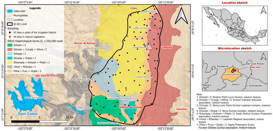
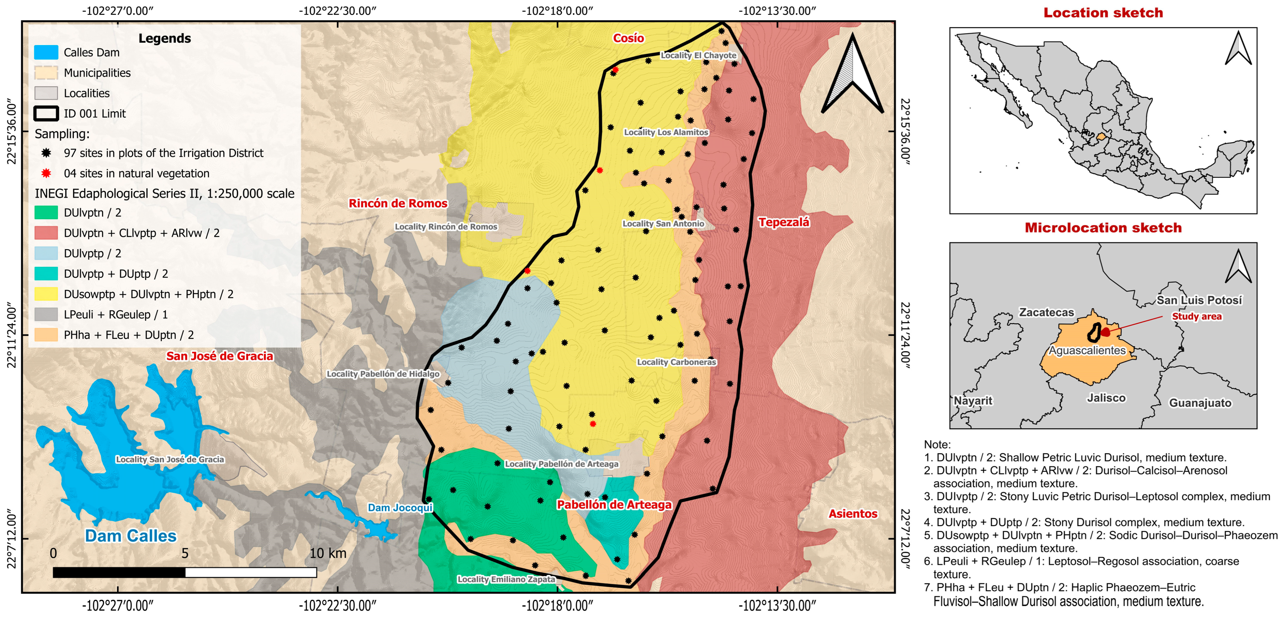
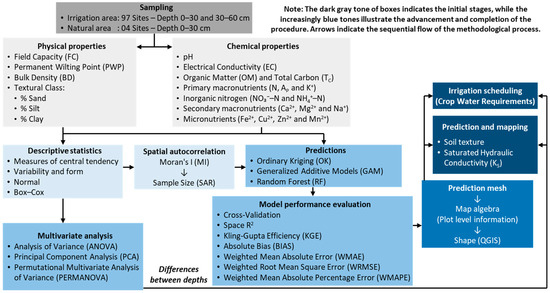
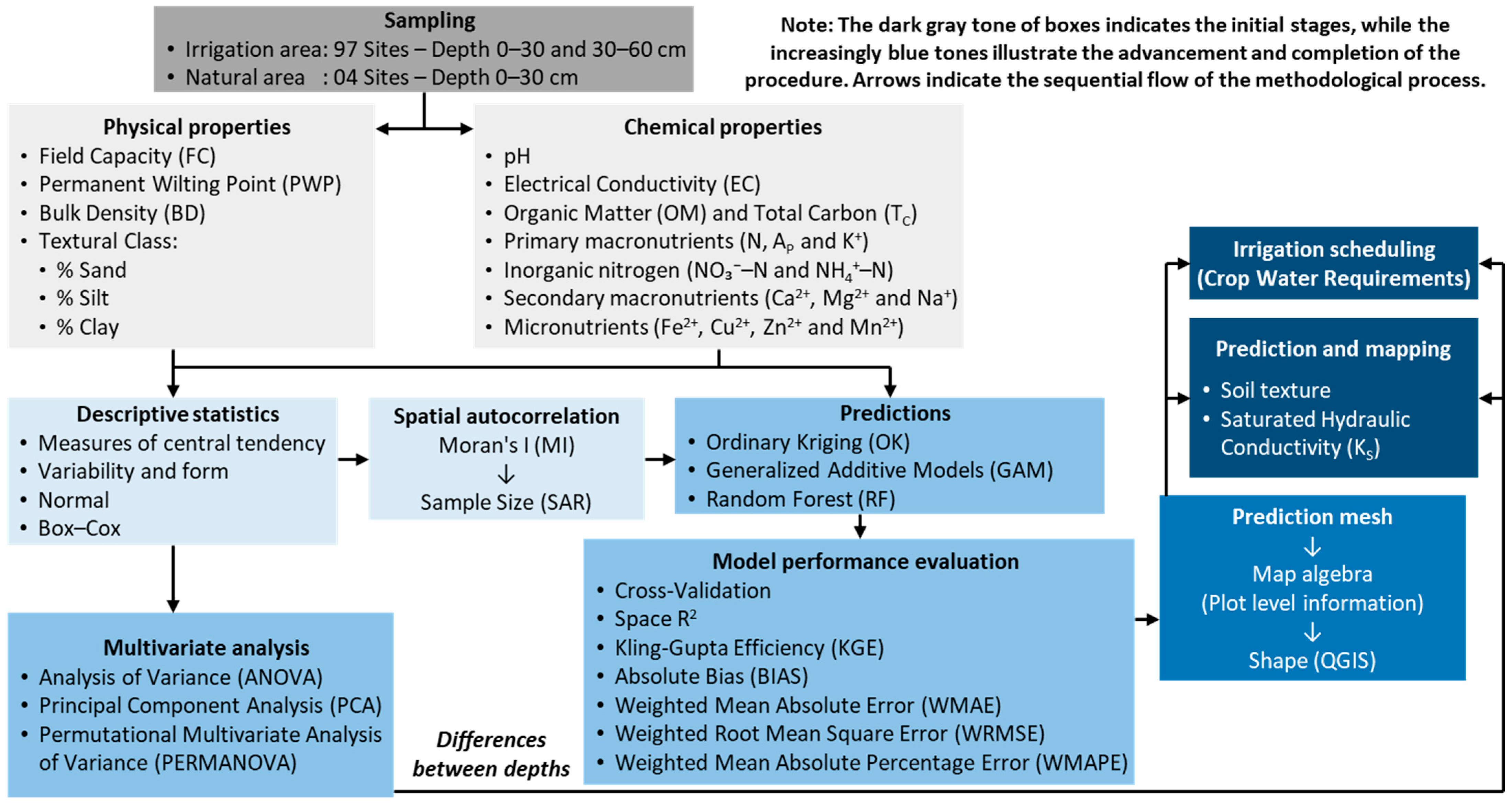
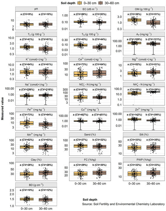
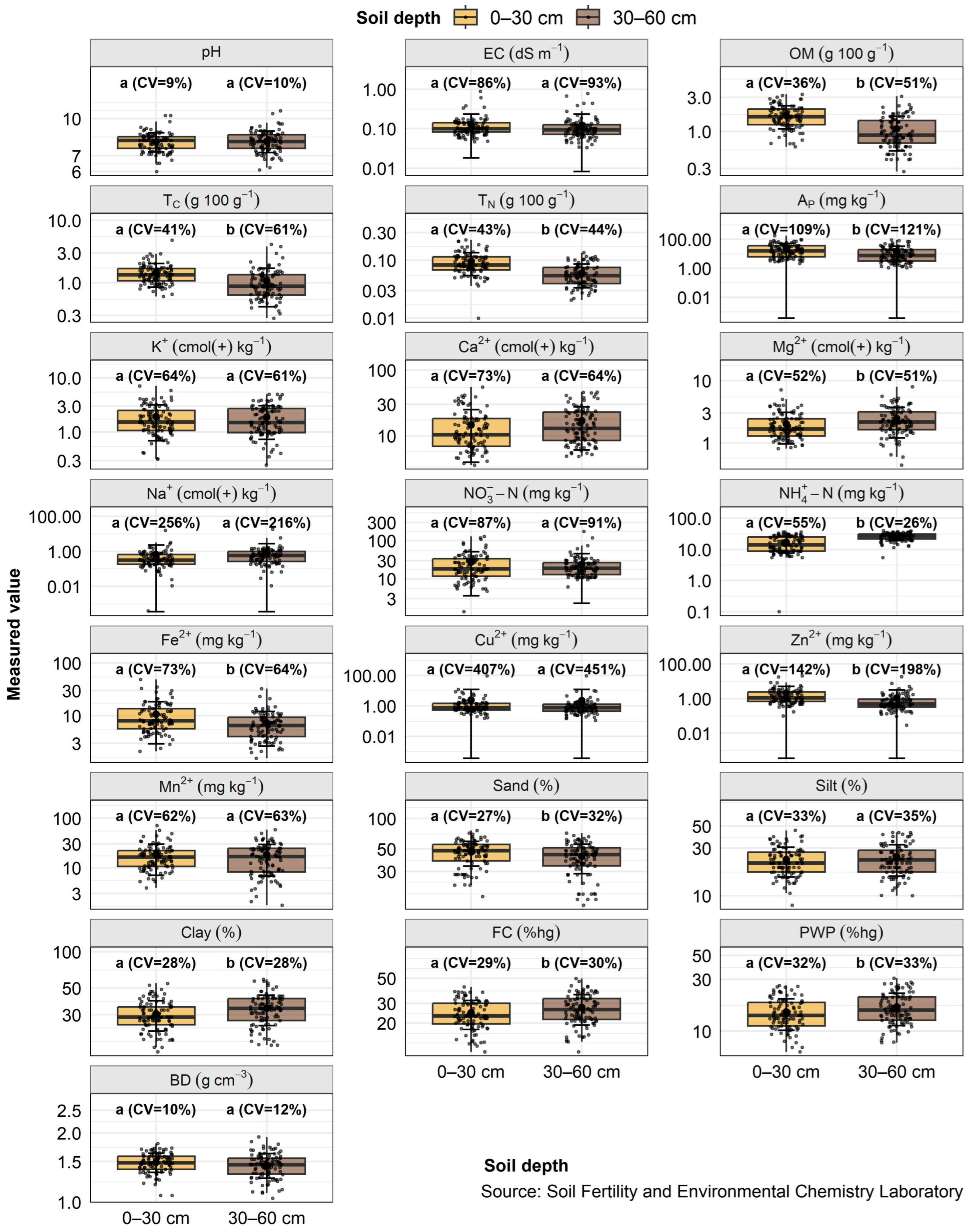
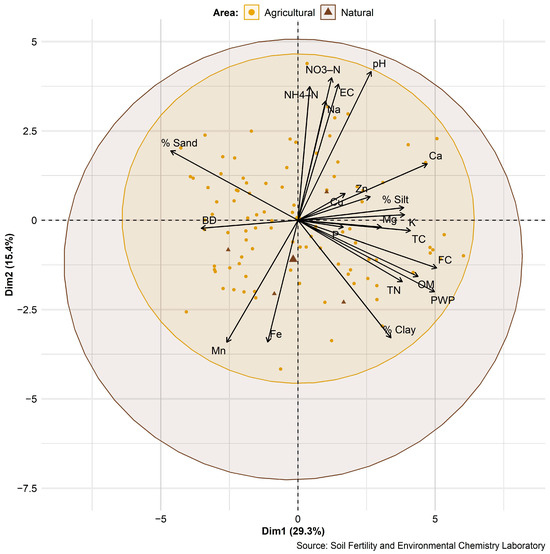
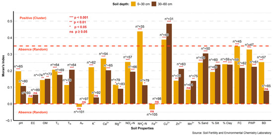
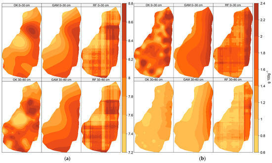
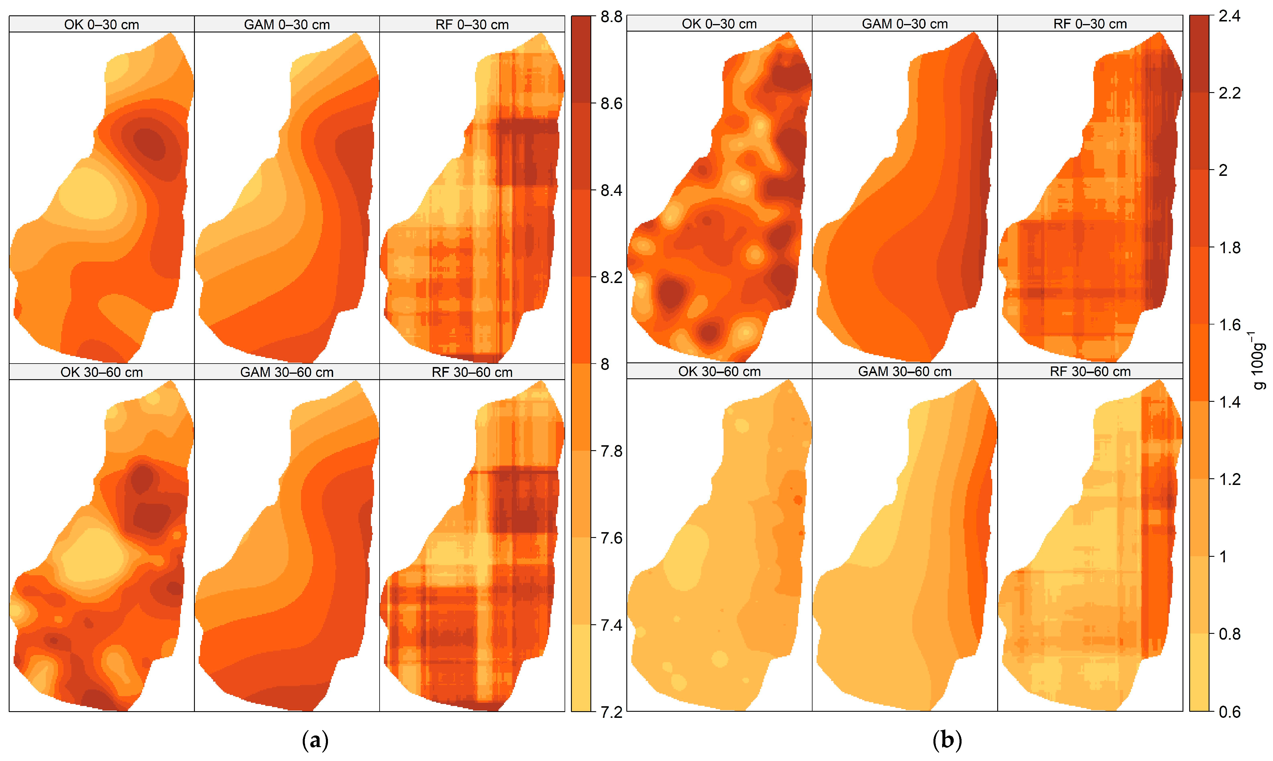
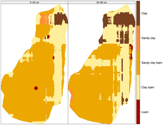
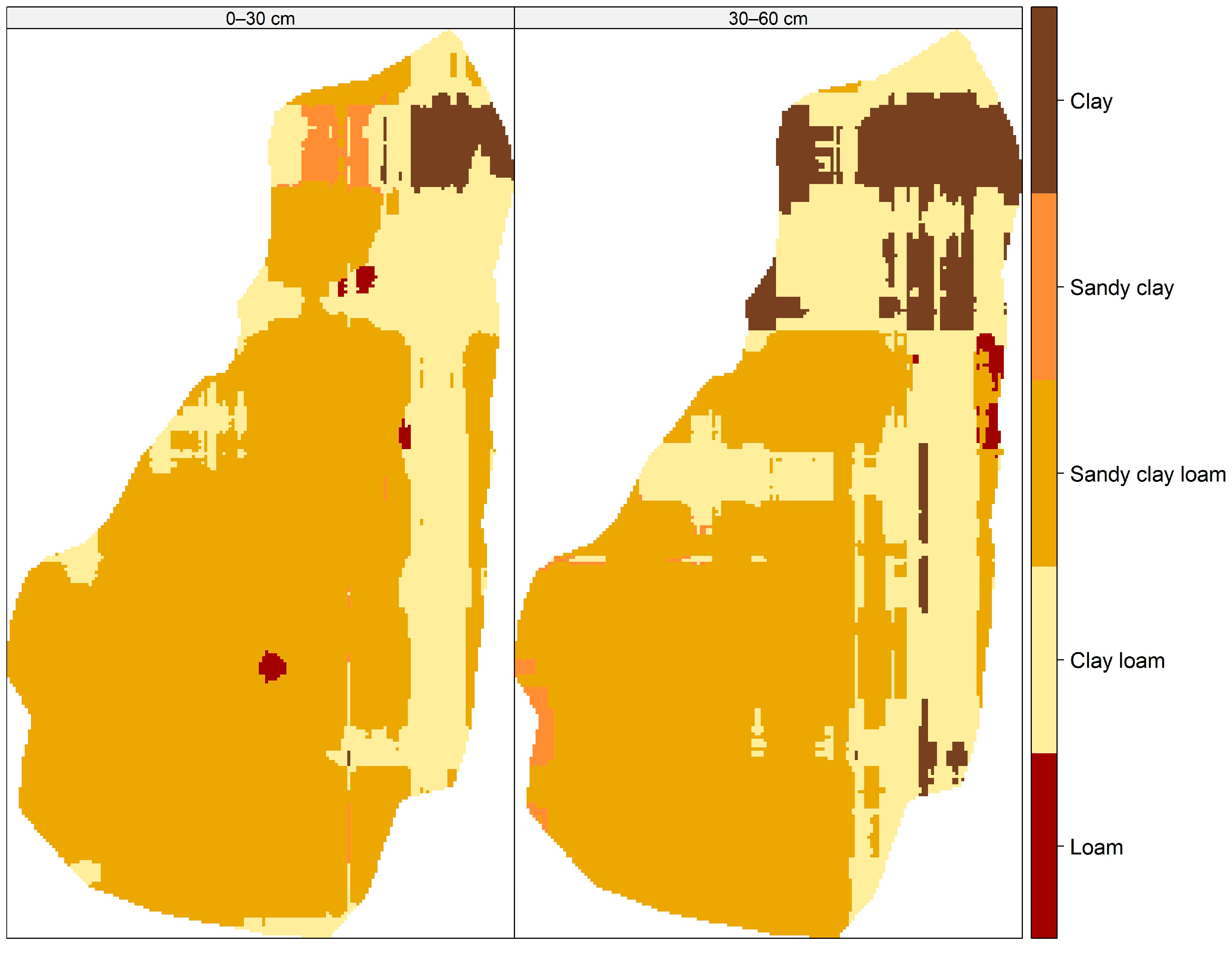
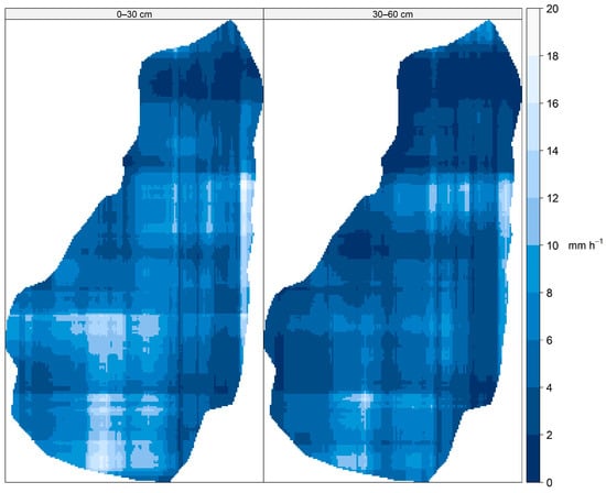
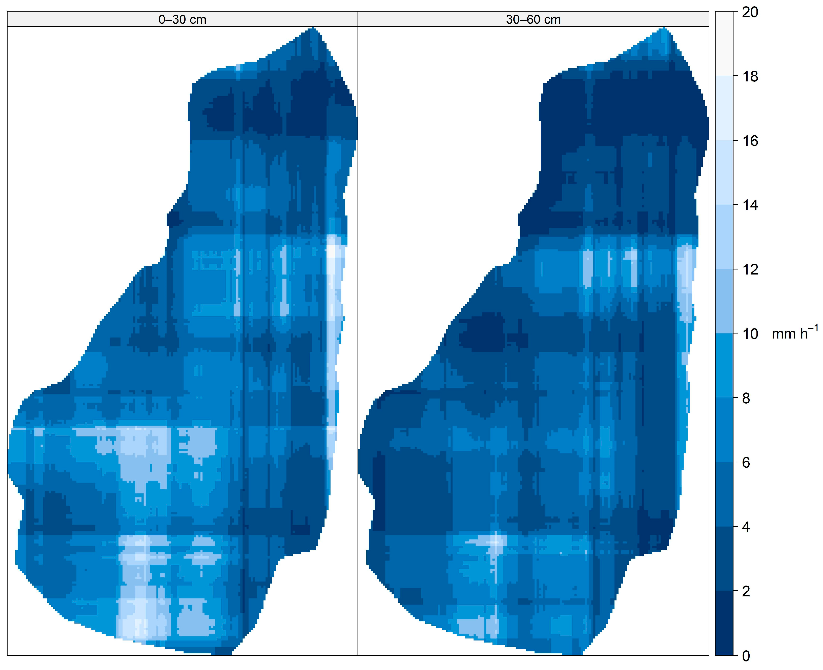
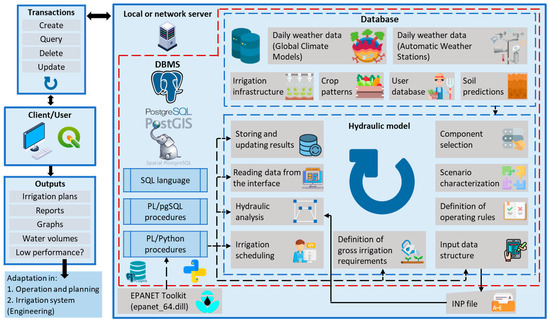
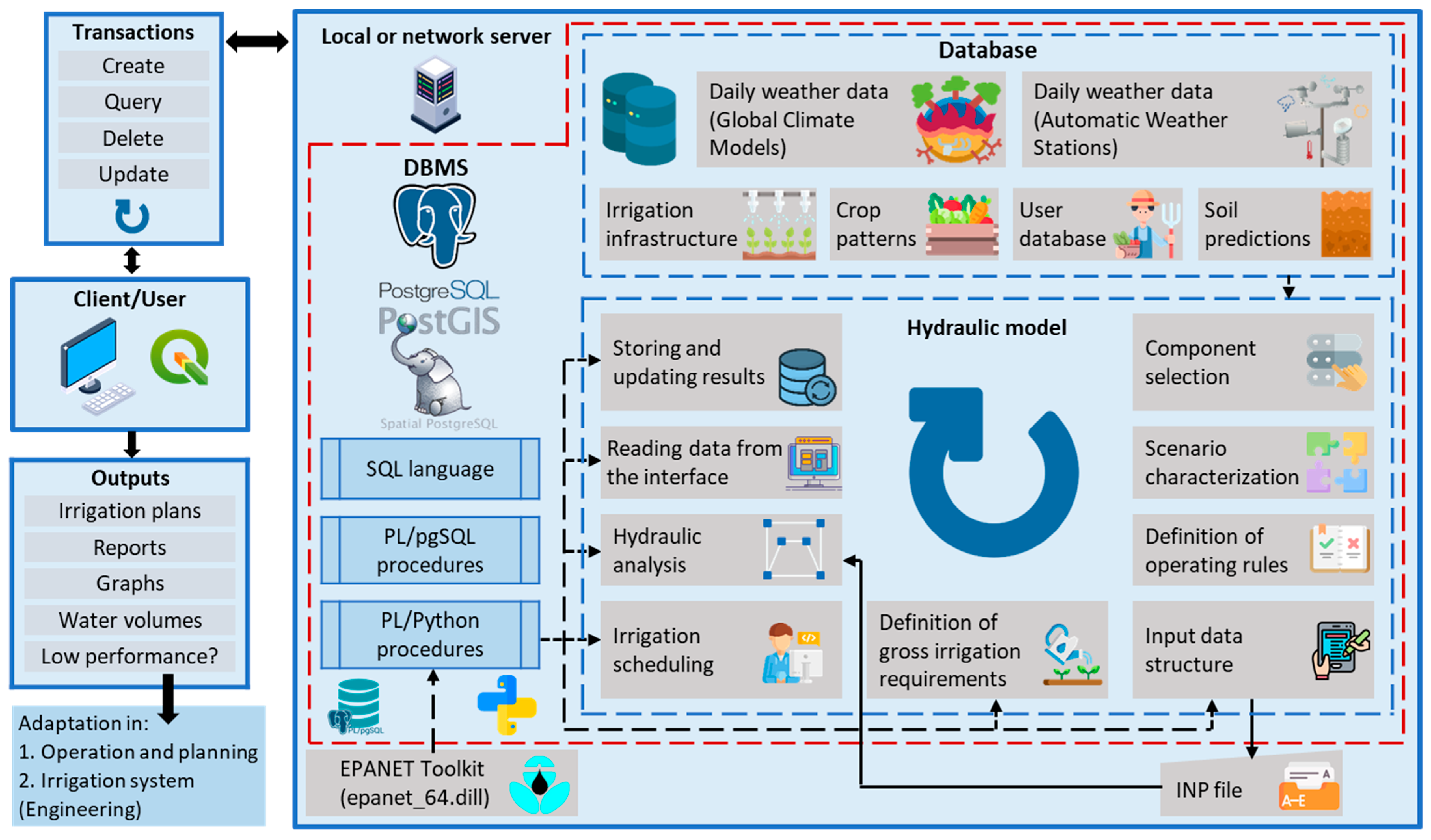

Disclaimer/Publisher’s Note: The statements, opinions and data contained in all publications are solely those of the individual author(s) and contributor(s) and not of MDPI and/or the editor(s). MDPI and/or the editor(s) disclaim responsibility for any injury to people or property resulting from any ideas, methods, instructions or products referred to in the content. |
© 2026 by the authors. Licensee MDPI, Basel, Switzerland. This article is an open access article distributed under the terms and conditions of the Creative Commons Attribution (CC BY) license.