


Abstract
This study examines the spatial imbalance and driving mechanisms of human–environment coupling in the Xiuhe River Basin, an important agricultural–ecological watershed in the middle and lower reaches of the Yangtze River. We integrated the coupling-coordination degree (C–D) model, Coupling Elasticity Index (CEI), spatial autocorrelation analyses (global and local Moran’s I, LISA, and Getis–Ord Gi*), and GeoDetector to assess spatial heterogeneity, classify coupling types, and identify key human–ecosystem. The results reveal marked spatial variation in coordination levels, which are higher in the central–western mountains and lower in the southeastern plains (global Moran’s I = 0.7344, p < 0.01), indicating significant spatial clustering. Using the CEI, the basin was classified into ecology-dominated zones (ecological advancement with human retreat), human-dominated zones (human advancement with ecological retreat), and relatively balanced zones. Upstream areas (CEI < 0.6) exhibit ecological advantages, whereas downstream plains (CEI > 1.5) experience dominant human pressures. GeoDetector analysis identified population density, proportion of built-up land, and water quality indicators (COD and TP) as the primary drivers, with interactions substantially enhancing explanatory power (e.g., PD × COD q = 0.86). These findings underscore nonlinear feedbacks and cross-scale interactions that influence coordinated ecosystem services in agricultural landscapes. We recommend differentiated management strategies: conserving upstream ecological functions, promoting balanced development in midstream areas, and regulating development intensity and pollution downstream to sustain human–environment coordination. This study provides quantitative evidence and methodological insights to improve understanding of ecological complexity and optimize governance of the agricultural landscape.
1. Introduction
The evolution of regional spatial patterns and their driving mechanisms has long been a central topic in geography, land science, and ecological planning [1,2]. Agricultural landscapes are typical coupled socio-ecological systems in which production functions and regulating services co-vary with land-use intensity and management [3]. Ecosystem services in such landscapes usually organize into explicit trade-offs, synergies, and bundles that can be diagnosed spatially rather than treated as independent outcomes [4,5]. Basin governance, therefore, requires interventions that enhance synergies while limiting key trade-offs under land–water constraints [6,7]. In recent years, spatial imbalance in human–environment systems has become a global concern and is regarded as a key challenge for land governance and sustainable development [8,9,10]. This problem is especially pronounced at the basin scale, where socioeconomic pressures and ecological constraints often intersect [11,12,13]. Uncovering the spatial patterns, typologies, and driving mechanisms of human–environment coupling imbalance in river basins is therefore essential for balancing development and conservation [14,15].
Extensive research has been carried out on human–environment coupling imbalance, leading to significant progress in several areas. Recent ecosystem-service studies in agricultural and peri-urban farming landscapes have used bundle identification and multifunctionality assessment to map where co-benefits and conflicts concentrate [4]. Scenario-based land-use or management analysis further quantifies how specific interventions shift the balance between provisioning outputs and regulating services [6,16]. These approaches provide an operational basis for linking spatial diagnosis to targeted measures in watershed planning [17]. In terms of imbalance pattern identification, researchers have continuously improved spatial statistics and hotspot analysis methods to enhance the accuracy of spatial heterogeneity assessments [18]. For example, recent studies have integrated coupling–coordination assessment with spatial autocorrelation and hotspot–coldspot diagnostics (e.g., global/local Moran’s I [19,20] and Getis–Ord Gi* [21]), and in some cases clustering algorithms, to reveal spatial clustering, polarization, and hotspot–coldspot structures in human–environment processes across different contexts [22,23,24]. Similar approaches have also been applied in the Huai River Basin, the Ili River Basin, and the Yangtze River Economic Belt, confirming that human–environment imbalance is characterized by significant spatial clustering and regional disparities [25,26,27,28]. These studies demonstrate that human–environment coupling imbalance is not randomly distributed but shows clear spatial polarization and regional differentiation.
With respect to imbalance type classification, research has gradually shifted from broad descriptions to more refined diagnostics. For example, studies have applied the coupling coordination degree (C–D) framework to identify differentiated coordination and imbalance types across development stages and regions, including urban agglomerations and national-scale land-use function systems based on multi-source heterogeneous data [9,29]. More recent work has further combined machine-learning models (e.g., random forest) with the C–D framework to simulate system changes and enable finer-grained recognition of imbalance types at local scales [30]. Collectively, these studies have promoted a transition in imbalance type classification from coarse descriptions at the macro scale to refined diagnostics supported by multi-scale and multi-method approaches.
With respect to driving mechanisms and interactions, increasing attention has been given to nonlinear effects and threshold phenomena.
For example, studies have used interaction-detection approaches (e.g., GeoDetector) to show that socioeconomic and ecological drivers often interact in a nonlinear manner, and that ecological responses under joint human–natural influences can exhibit nonlinear enhancement rather than linear superposition [1,2,31]. Evidence from basin-scale analyses further suggests that when socioeconomic or environmental pressures exceed critical levels, imbalance risks can rise sharply, highlighting the policy relevance of threshold effects in watershed governance [32]. These findings indicate that human–environment system imbalance is often driven by multiple interacting factors and is characterized by distinct threshold effects and nonlinear dynamics.
Collectively, existing studies have accumulated substantial achievements in pattern identification, type classification, and driving mechanism analysis, which have greatly advanced research on coupling imbalance patterns [33,34]. However, much of this work remains confined to a single dimension and lacks an integrated framework that systematically links patterns, types, and mechanisms [35,36,37]. Although the ecosystem-service literature has offered actionable evidence on bundles, multifunctionality, and scenario responses, it is still weakly integrated with coupling-imbalance diagnostics at the basin scale [4]. As a result, the synergy–trade-off logic is not yet fully translated into an imbalance-oriented chain that directly supports zoning, threshold-based intervention, and policy sequencing in agricultural basins [6,17]. In addition, policy support is insufficient, as few studies translate empirical results into differentiated governance strategies at the basin scale, which limits their practical applicability [38,39].
This study took the Xiuhe River Basin, an important tributary of the middle and lower Yangtze River, as a case study. It developed an integrated analytical framework that combined the C–D model, the Coupling Elasticity Index (CEI), spatial autocorrelation analysis, and the GeoDetector model. The framework was used to systematically diagnose the spatial patterns of human–environment coupling imbalance, classify relationship types, identify the main driving mechanisms, and explore differentiated governance scenarios. By establishing an analytical loop of type identification, mechanism analysis, and threshold testing, the study provides empirical support for zoned, targeted, and coordinated governance, and offers theoretical insights and practical references for promoting human–environment coordination in similar basins.
This study cautioned that a very high coupling degree does not necessarily indicate a sustainable human–environment relationship. By jointly interpreting coupling (C), coordination (D), and CEI, the analysis avoided conflating interaction intensity with ecological well-being. The study further provided basin-scale threshold evidence showing that coordination losses accelerate once key socio-economic and pollution pressures cross upper-quantile strata; for example, when population density and COD jointly exceed the third quantile, declines in D become markedly larger. Finally, these threshold signals were translated into operational zoning and intervention priorities by linking quantile transitions to expected marginal improvements in coordination; in high-load townships, reducing COD from the highest quantile stratum to the next was associated with an average increase in D of more than 0.06.
This paper is organized as follows: Section 2 introduces the study area and data sources. Section 3 describes the materials and methods, including indicator systems and analytical diagnostics. Section 4 presents the results. Section 5 discusses the findings and limitations. Section 6 concludes the study.
2. Study Area and Data Sources
2.1. Study Area
The Xiuhe River Basin (Figure 1), located in the northwestern part of Jiangxi Province, is one of the five major sub-basins of Poyang Lake, the largest freshwater lake in China. The main stream of the Xiuhe River originates from Xiadong, Huanglong Mountain Village, in the Mufu Mountains, with a drainage area of 14,700 km2. It flows into Poyang Lake at Wangjiang Pavilion in Wucheng Town, covering a mainstream length of 389 km. Major tributaries include the Dongjinshui River and the Liaohe River. The section above Xiushui County is regarded as the upper reaches; below Zhelin Reservoir, the river enters the lower reaches; and downstream of Yongxiu County, it flows into the lakeside polder area, where the current is slow, and backflow from Poyang Lake during flood season often causes inundation. The Liaohe River, the largest tributary of the Xiuhe, diverges from the main stream at the Jiuling Mountains, with a catchment area of 4333 km2 and a mainstream length of 148 km. At Shiwuo in Anyi County, it splits into the Nanliao River (catchment area of 1929 km2) and the Beiliao River (catchment area of 1542 km2). The catchment area above the Wanjia Bu control station reaches 3548 km2, with three medium- to large-sized reservoirs within the basin. The Zhelin Reservoir, the largest in Jiangxi Province, is situated in the middle and lower reaches of the Xiuhe River, controlling a drainage area of 9340 km2. The basin covers the counties of Yongxiu, Wuning, Xiushui, Jing’an, and Anyi, accounting for 9.1% of the total Poyang Lake Basin area. The long-term average annual inflow from the Xiuhe River into Poyang Lake is 14.4 × 10⁹ m3, representing 11% of the total inflow from the five rivers and 9.4% of the entire basin’s inflow.
Figure 1.
Regional location map. Notes: All maps were produced in the China Geodetic Coordinate System 2000 (CGCS2000), EPSG:4490; the same CRS applies to all other map figures in this manuscript.
2.2. Data Sources
The basic data required for this study encompass two main aspects: natural ecology and socio-economic conditions, all referenced to the year 2024.
(1) Natural ecological data: Land-use maps (including categories such as cultivated land, forest land, and water bodies) were obtained through the interpretation of multi-source remote sensing imagery, from which ecological indicators such as the NDVI were calculated. Hydrometeorological data (e.g., precipitation, runoff) as well as soil and topographic data (e.g., DEM) were also collected. Remote sensing data were mainly derived from Sentinel-2 and Landsat-8 imagery and were processed through radiometric correction, atmospheric correction, and manual interpretation.
(2) Human activity data: These were collected from statistical yearbooks of counties and cities within the basin, including indicators such as population, GDP, land-use intensity, water quality monitoring data, and industrial wastewater discharge. Administrative boundary vector data were used for spatial clipping, while socio-economic point data were applied in spatial analyses. All spatial datasets were standardized to the CGCS2000 coordinate system.
3. Materials and Methods
3.1. Indicator System for Evaluation
Following the general framework of human–land system coupling research, this study decomposed the human–land system into two subsystems: the human activity subsystem and the natural ecological subsystem. Based on the regional characteristics of the Xiuhe River Basin and data availability, representative indicators were selected to characterize the state of each subsystem. The indicator system was designed in line with the principles of scientific rigor and simplicity, encompassing both human elements (e.g., population, society, and economy) and natural elements (e.g., land, resources, and environment).
To clarify the linkage to resource–environmental carrying capacity and spatial suitability in an agricultural watershed, the indicators selected represented a pressure–state/response logic. Specifically, the human activity subsystem focuses on development intensity and pressure pathways that directly alter land–water processes, including population agglomeration, built-up expansion, socio-economic activity, and pollution loads generated by human production and living activities. The natural ecological subsystem represents ecological state, support capacity, and constraint conditions that determine where intensive use can be sustained, including vegetation productivity, soil fertility and erosion risk, hydrological regulation, habitat integrity, and landscape structure. This design enables the coupling results to be interpreted as the spatial manifestation of “development pressure versus ecological carrying/suitability constraints”, rather than a purely statistical association.
(1) Indicators of the human activity subsystem: These primarily measure the level of population and socio-economic development in the region, reflecting the pressure exerted on land use and the intensity of human impacts. Following recent indicator-setting practices in human–environment coupling and basin studies, where population density and nighttime light are commonly used to proxy development intensity and human activity pressure [40,41], and nighttime-light-based approaches are widely adopted to capture built-up expansion patterns [42], population density (PD), enterprise density (ED), the proportion of built-up area (PBA), and nighttime light index (NLI) jointly describe human development intensity and spatial agglomeration, which are commonly regarded as direct proxies for demand pressure and land conversion intensity in basin governance. COD, TP, NH3-N, and industrial wastewater discharge (IWD) are included to capture pollution-load pathways that translate development intensity into water-quality stress, because water pollution in agricultural basins often acts as the main conduit through which human activities constrain ecological functioning and carrying capacity. The specific design of the indicator system is shown in Table 1.
Table 1.
Indicators of the human activity subsystem.
(2) Indicators of the natural ecological subsystem: These capture the regional resource–environment conditions and ecological support capacity, reflecting the land’s carrying capacity and feedback to human activities (Table 2). Following recent basin-scale ecological quality and watershed assessment studies that operationalize ecological support and suitability using vegetation productivity, soil condition/erosion risk, hydrological regulation, and landscape structure/connectivity metrics [43,44], NDVI and NPP indicate vegetation condition and primary productivity, representing ecosystem vigor and potential service supply. LEQI synthesizes land-use patterns, vegetation conditions, and hydrological contexts to characterize overall ecological quality in an integrated manner. SOM reflects soil fertility and buffering capacity, while WRC captures hydrological regulation and water conservation capacity that is critical for agricultural landscape stability. SEV measures degradation pressure through soil loss, and FI and EC characterize landscape fragmentation and ecological connectivity, which constrain habitat integrity and the persistence of ecological processes. BDI complements structural indicators by reflecting habitat-related diversity potential. Together, these indicators describe both ecological support capacity and spatial suitability constraints that shape coordination outcomes under agricultural landscape pressures.
Table 2.
Indicators of the natural ecological subsystem.
3.2. Analytical Methods
(1) Conceptual framework and analytical logic
Human–environment coupling in an agricultural watershed is more than statistical co-variation between human activities and ecological conditions. It can be understood as a process chain in which development intensity generates pressure pathways, triggers ecological responses, and ultimately shapes coordination outcomes. Accordingly, the analysis followed a concise conceptual logic (Figure 2): (1) human development intensity (e.g., population concentration, built-up expansion, and socio-economic agglomeration) elevates resource demand and accelerates land-use conversion; (2) these changes translate into pressure pathways, notably pollutant loads and landscape transformation, which modify hydrological and ecological processes; (3) the system exhibits ecological responses reflected by environmental conditions and ecosystem service-related indicators; and (4) the joint dynamics of the human and ecological subsystems emerge as coordination outcomes, quantified through coupling–coordination metrics.
Figure 2.
Conceptual framework of human–environment interactions and analytical diagnostics.
Within this logic, the coupling degree (C) describes the strength of interdependence between the two subsystems. Crucially, a high C indicates interaction intensity rather than ecological well-being; tightly linked systems may still experience severe stress. Therefore, C is interpreted jointly with the coordination degree (D) and a dominance diagnostic. To distinguish “strong interaction” from “balanced development”, the comparative equilibrium index (CEI) is employed as a relative dominance measure (H/E), suggesting whether the human subsystem advances faster than the ecological subsystem (human-dominant) or vice versa (ecology-dominant). CEI is thus treated as a trajectory-oriented indicator of subsystem imbalance rather than an absolute ecological threshold.
To translate the conceptual chain into policy-relevant evidence, quantile-based threshold diagnostics are further introduced. Rather than assuming smooth linear responses, the threshold analysis tests whether coordination outcomes (D) change disproportionately when key pressures (e.g., development intensity and pollution loads) shift from lower to higher strata. These quantile strata are interpreted as relative risk levels within the basin, enabling consistent comparison across indicators and townships. In combination, the framework links (i) indicator construction and coupling–coordination assessment, (ii) spatial dependence diagnostics, (iii) driver identification and interaction assessment, and (iv) threshold-informed scenario implications into a coherent, mechanism-aware analytical logic, thereby reducing the risk of a purely mechanical assemblage of tools.
Following the above logic, the analysis first constructs the human and ecological indicator systems and quantifies C, D, and CEI, and then diagnoses spatial dependence patterns, dominant drivers, and quantile-based threshold responses.
(2) Coupling Degree and Coupling Coordination Degree
The above indicators were standardized, with those of the human activity subsystem transformed into dimensionless values within the range of 0–1 using min–max normalization, while the indicators of the natural ecological subsystem were also standardized. To reduce subjective bias, the entropy weight method was applied to calculate the weights of the indicators. Weighted summation was then performed to obtain the development index of the human activity subsystem and the development index of the natural ecological subsystem, as expressed in the following formula [45]:
In Equations (1) and (2), and represent the number of indicators included in the two subsystems, while and denote the indicator weights (satisfying ). and are min–max standardized indicator values (0–1), and and are the corresponding dimensionless composite development indices.
The coupling degree model was introduced to quantitatively evaluate the interactive coordination between the two subsystems. C reflects the closeness of their interaction, and its improved physical coupling function can be expressed as [46]:
In Equation (3), C ranges from 0 to 1, with values closer to 1 suggesting that the human and ecological subsystems develop in a more synchronized manner, while lower values suggest asynchronous development and a state of imbalance or separation. Nevertheless, the coupling degree alone cannot fully capture the quality of human–environment relationships; thus, the comprehensive coordination index (T) [47] and the coupling coordination degree (D) [47] are introduced to evaluate the overall development level of the system:
In Equations (4) and (5), T denotes the overall development level of the human–land system, while α and β are weighting coefficients. The coefficients and were set to 0.5 to assign equal importance to the two subsystems. D integrates both the degree of coupling and the overall development level, which ranges from 0 to 1. A higher D value indicates that the human–land system is not only tightly coupled but also at a relatively advanced stage of development, reflecting a state of coordinated optimization. Conversely, a lower D value suggests that the system either remains underdeveloped or suffers from imbalance, representing an uncoordinated state. By jointly evaluating C and D, the human–land relationship within the basin can be more comprehensively assessed. The joint use of C and D is intended to distinguish interaction intensity from coordination outcomes, thereby improving interpretability in cases where high coupling may coexist with low coordination.
Building on the above indicators, this study introduces the Coupling Elasticity Index (CEI). The C–D model can measure the overall coordination level of the human–environment system, but its results tend to be averaged, which may obscure regional differences and asymmetries. In contrast, the CEI compares the relative rates of change between human activities and the ecological environment, and thus better reveals the strength of relationships such as “human expansion and ecological retreat” or “ecological advance and human retreat.” In practice, CEI is formulated as the ratio of the composite development levels of the two subsystems, which is consistent with the widely used “relative development degree” (RDD) idea that complements the coupling–coordination assessment by identifying which subsystem is relatively leading or lagging. Recent studies in authoritative journals have employed the same ratio logic together with the CCD framework to distinguish “system balanced” versus “one-side lagging” states, thereby avoiding the misinterpretation that high coupling necessarily implies high coordination [48]. Following this literature, CEI is used here as a structural diagnostic that highlights dominance and asymmetry between human and ecological subsystems, while C and D summarize interaction intensity and overall coordination [48]. This complementarity allows the two models to jointly reflect both the overall coordination level and the structural imbalance of the system, providing more comprehensive support for identifying different types of human–environment relationship patterns.
In Equation (6), CEI reflects the relative dominance between the human and ecological subsystems. When CEI > 1, it indicates that the level of human development surpasses the ecological environment, suggesting a tendency toward a human-advancing/ecology-retreating imbalance. When CEI < 1, it reflects the opposite pattern, namely an ecology-advancing/human-retreating configuration. A CEI value close to 1 implies that the two subsystems develop in a generally synchronized and balanced manner. Thus, CEI provides a quantitative means to distinguish different types of human–land imbalance across regions, offering a basis for identifying potential ecological risk areas.
To further analyze the spatial differences in human–land coupling across different regions of the basin, both C and D were classified into categories. C was divided into five levels: very low coupling, low coupling, moderate coupling, high coupling, and very high coupling. Similarly, D was classified into five levels: very low coordination, low coordination, moderate coordination, high coordination, and very high coordination. The classification thresholds were determined using the natural breaks (Jenks) method based on the distributional characteristics of the data.
(3) Spatial diagnostics
ArcGIS (version 10.8) was used to visualize the spatial distribution of the coupling coordination degree, with color gradients applied to reflect regional differences in magnitude. To characterize spatial structure and explain its drivers, spatial diagnostics were conducted from three complementary perspectives: (i) hotspot intensity of human activities, (ii) spatial dependence of coordination outcomes, and (iii) factor attribution and interactions.
Kernel density estimation (KDE) was applied to population and built-up land to identify hotspots of human activity [49]. KDE was applied to population and construction land to identify spatial hotspots of human activities, thereby providing auxiliary insights into the spatial differences in the human–land coupling pattern. Key KDE settings (e.g., bandwidth and kernel type) followed ArcGIS (version 10.8) defaults and were kept consistent across the basin to ensure comparability among township units.
To determine the spatial clustering of the coupling coordination degree, the global Moran’s I index was calculated to examine the overall spatial pattern of coupling coordination across the basin. Global Moran’s I was computed based on the township spatial weight matrix to test whether D exhibits significant spatial dependence at the basin scale. A significantly positive I value indicates the presence of spatial clustering, where high-value or low-value regions tend to be adjacent in space. Local spatial association (LISA) and hotspot diagnostics were then used in the results to locate high–high and low–low clusters and to support spatial zoning interpretation.
The GeoDetector method was employed to identify the importance of human activity driving factors and to test their interactive effects. GeoDetector was applied to quantify the explanatory power (q-statistic) of each potential driver on the spatial variation in D and to assess whether paired factors exhibit enhanced or weakened interaction effects [50]. A larger q-value indicates a stronger explained variance contribution of the factor for the coupling coordination degree. Factor stratification followed the standard GeoDetector procedure by discretizing continuous variables into categorical strata (consistent across factors) to ensure comparability of q-statistics and interaction detection.
(4) Threshold analysis
The conditional mean method was used to identify the responses of the human–environment coupling coordination degree across different quantile levels of driving factors. Quantile-based thresholds were adopted to diagnose non-linear responses in coordination under heterogeneous socio-economic and environmental contexts. For most drivers considered in this study (e.g., population density, built-up intensity, and composite pressure indicators), universally applicable policy benchmarks or ecological limit values are either unavailable, defined in incomparable units, or highly context-dependent across geomorphic and hydrological settings. In contrast, equal-frequency quantile stratification provides a consistent, data-driven way to classify drivers into relative pressure levels within the basin while maintaining comparable sample sizes across strata, which stabilizes the estimation of the conditional mean of the coordination degree and facilitates interpretation across multiple drivers. By dividing each factor into several quantile intervals and calculating the mean coordination degree within each interval, the method can reveal system responses under different levels of pressure. When the coordination degree shows a significant decline after crossing a specific quantile, it is regarded as evidence of a potential threshold effect. The quartiles are used here as relative risk benchmarks rather than as absolute ecological standards or direct policy boundaries. The resulting “thresholds” should be interpreted as suggesting ranges in which coordination exhibits a noticeably different response as drivers move from one relative level to another within the basin. Unlike traditional linear regression or correlation analysis, the conditional mean method provides a more intuitive way to capture nonlinear changes and to identify the critical states of the human–environment system. Accordingly, the diagnostics help identify factor ranges associated with noticeably different coordination responses, supporting the prioritization of intervention and spatial zoning within the basin.
Assume that the coupling coordination degree is denoted as and the driving factor as . The variable is divided into several quantile intervals. For each quantile interval , the conditional mean of is calculated as
In Equation (7), is the mean coordination degree within stratum , is the number of townships in that stratum, and is the coordination degree of township . denotes the set of townships whose driver value falls in the -th quantile stratum. Quantile strata were constructed for each driver using equal-frequency grouping within the basin.
(5) Robustness, validation, and bias management
To strengthen validation and manage potential methodological biases, we conducted robustness and stability checks for the C and D by perturbing two key sensitivity sources while keeping the indicator set and the coupling–coordination formulation unchanged: (i) the weighting scheme used to aggregate indicators into the human-activity and ecological-environment subsystem indices, and (ii) the preference parameter α in the coordination formulation. For each setting, C and D were recalculated at the township level, and stability was evaluated using rank consistency, absolute deviations, and extreme-group agreement.
For weighting robustness, we compared the baseline results with three alternative schemes, including equal weights, re-estimated entropy weights, and PCA weights. Stability was assessed using Spearman rank correlation and Pearson correlation, mean absolute deviation (MAD), root mean square error (RMSE), and overlap rates of the top and bottom deciles of D under alternative schemes.
For parameter sensitivity, α was varied within a plausible range to test whether the basin-wide ordering of D and the composition of extreme groups remained stable. In addition, to ensure the stability of the classification used for mapping and zoning interpretation, we quantified the agreement rate of five-quantile grades under alternative weighting schemes.
4. Results
4.1. Coupling Coordination
4.1.1. Coupling and Coordination
According to the results of the coupling coordination model, the average coupling degree of the Xiuhe River Basin was 0.965, close to the theoretical upper limit of 1. This result indicates strong interdependence and intensive interactions between the human activity subsystem and the natural ecological subsystem, rather than inherently implying a healthy or well-coordinated system. Therefore, we interpret C jointly with D and CEI in subsequent analyses. The interpretation of C is therefore complemented by the coordination degree (D) and the dominance diagnostic (CEI) in subsequent analyses. In terms of spatial distribution, the maximum coupling degree reached 1, observed in township-level units located in the middle and upper mountainous areas of the basin, whereas the minimum value was only 0.790, mainly concentrated in the downstream plain region (Figure 3a).
Figure 3.
Coupling degree (C), coordination degree (D) and coupling elasticity index (CEI) in the Xiuhe River Basin: (a) C; (b) D; (c) CEI.
The average D of the Xiuhe River Basin was 0.710, representing a moderately high level of coordination. In this study, the maximum observed value was 0.932, approaching the state of ideal coordination, and was mainly distributed in agricultural townships in the middle and upper reaches of the basin. The minimum value, 0.339, occurred in downstream towns and agricultural plain townships, where significant human–land discordance was evident. Overall, the majority of townships exhibited “basic coordination” or “moderate coordination,” while only a few areas showed patterns of imbalance or low coordination (Figure 3b).
From the perspective of the relative relationship between the subsystems, the average CEI value across the Xiuhe River Basin was 1.437, but with pronounced spatial differences (Table 3). Beyond categorical interpretation, higher CEI values indicate that human-system advancement outpaces ecological-system improvement by a larger margin, implying a growing imbalance in relative change rates. In the upstream and southern areas of the basin, township-level CEI values were less than 1 (the lowest being 0.519), indicating that the ecological subsystem is more advanced than the human subsystem, resulting in an “ecology-advancing/human-retreating” pattern. In contrast, the valley corridors and the northeastern outflow areas formed stable high-value clusters, reflecting a trend of “human-advancing/ecology-retreating” (Figure 3a,b). In townships with very high CEI (e.g., approaching 4), human expansion may proceed several times faster than ecological recovery or improvement, implying elevated long-term risks of accumulated degradation even when short-term coordination remains moderate. In most regions, the CEI was close to 1, suggesting that human and ecological developments are largely synchronized and the coordination relationship remains relatively stable (Figure 3c).
Table 3.
Summary statistics of overall coupling coordination levels.
4.1.2. Coupling Coordination Classification
Using the natural breaks (Jenks) method, both C and D were classified. In this study, the classes were uniformly divided into five categories: very low, low, moderate, high, and very high. The corresponding class thresholds and township counts are summarized in Table 4 and Table 5, and their spatial patterns are shown in Figure 4.
Table 4.
Statistical summary of coupling degree classification.
Table 5.
Statistical summary of coordination degree classification.
Figure 4.
Classification map: (a) coupling degree; (b) coordination degree.
(1) Coupling Degree Classification
The overall range of C was 0.790–1.000, and the classification results are presented in Table 4 and Figure 4a. Overall, C was dominated by the “high” and “very high” classes (Table 4), accounting for 72 townships (66.67%), suggesting intensive human–land interactions across most areas. The very high coupling zones were mainly distributed in a belt-like pattern across the southern high-altitude areas of the basin, typically located in the southern part of Xiushui County, the eastern part of Tonggu County, and the central–western mountainous–hilly transition zones of Jing’an County. In contrast, areas with lower coupling degrees were largely concentrated in the downstream plains, such as Yongxiu County and the northeastern part of Wuning County. The coupling degree reflects both the intensity and the degree of matching between the two subsystems. In the southern high-altitude areas, relatively lower development intensity tended to be more compatible with ecological conditions, whereas in downstream plains and river-valley areas, high development intensity coincided with comparatively weaker ecological conditions, resulting in a more mismatched structure.
(2) Coordination Degree Classification Results
D ranged from 0.339 to 0.932, with an average value of 0.710. Based on the natural breaks method, the five-level classification results are presented in Table 5 and Figure 4b. In contrast to the uniformly high coupling, D exhibited clearer stratification across classes (Table 5), with low-coordination townships primarily concentrated in the downstream plains. The “high” and “very high” coordination zones were mainly distributed in the southern part of the basin, including Tonggu County, the southern part of Xiushui County, the entire area of Jing’an County, and the southern and northern high-altitude and mid-to-high-altitude mountainous areas of Wuning County. These regions had relatively favorable ecological backgrounds and moderate development intensity, where the alignment between H and E was relatively strong, presenting a state of “factor matching—positive interaction—high coordination.” In contrast, the “low” and “very low” coordination zones were concentrated in the downstream plains of the basin, such as Anyi County, the eastern part of Fengxin County, and the southeastern part of Yongxiu County. These low-coordination areas generally reflected either high development pressure accompanied by ecological stress, or relatively favorable ecological conditions but insufficient industrial and population agglomeration; in both cases, coordination deficits indicate tension between carrying capacity and development intensity.
4.1.3. Spatial Clustering Characteristics
(1) Global Moran’s I
Using the township-level D as the analysis variable, a global spatial autocorrelation test was conducted with the ArcGIS (version 10.8) Spatial Autocorrelation (Global Moran’s I) tool. The results showed Moran’s I = 0.7344, z = 11.9924, p < 0.01; Expected I = −0.0093, Variance = 0.0038. This indicates that the coordination degree across the basin was significantly and positively spatially autocorrelated, with high-value areas clustering with high-value areas and low-value areas clustering with low-value areas, forming a clear spatial aggregation pattern. Overall, the results confirm a strong and statistically significant basin-wide clustering pattern of D, providing a basis for subsequent local cluster and hotspot diagnostics. The results are presented in Table 6 and Figure 5.
Table 6.
Summary statistics of global Moran’s I.
Figure 5.
Significance diagram of global Moran’s I.
(2) Local Moran’s I
The local Moran’s I (LISA) was applied to further analyze the spatial clustering and outlier distribution of coordination in the Xiuhe River Basin, with the results shown in Figure 6a. The analysis identified a total of 16 townships of the high–high (HH) cluster type, mainly distributed in the central and southwestern mountainous areas of the basin. Representative HH townships included Manjiang Township, Fuyuan Township, and Wenquan Town, suggesting contiguous areas with consistently high coordination. A total of 13 townships were identified as low–low (LL) clusters, primarily located in the southeastern downstream region of the basin. Representative LL townships included Tubu Town, Dinghu Town, and Huangzhou Town, forming contiguous low-coordination clusters. High–low (HL) and low–high (LH) types did not reach significant levels in this analysis, with few isolated high- or low-value units observed. Overall, the coordination degree in the Xiuhe River Basin presents a spatial pattern of high-value clustering in the central and western areas and low-value clustering in the southeastern areas. These results indicate that coordination deficits are spatially concentrated rather than randomly distributed, supporting geographically differentiated improvement strategies.
Figure 6.
Local spatial clusters and hotspot–coldspot patterns of coordination degree (D): (a) LISA; (b) Getis–Ord Gi*.
(3) Getis-Ord Gi* Hotspot Analysis
To further identify the significant high- and low-value clusters of coordination in the Xiuhe River Basin, the Getis-Ord Gi* hotspot analysis was employed to conduct spatial clustering tests. In the analysis, D was used as the research variable, the threshold distance was determined by average nearest neighbor analysis, and a spatial weight matrix was constructed using the contiguity (shared-border) method. The results are shown in Figure 6b. The analysis reveals significant hotspot–coldspot structure across the basin. Specifically, a total of 21 townships were identified as hotspots, mainly concentrated in the western and central mountainous areas. Hotspots included Manjiang Township, Fuyuan Township, and Wenquan Town, forming spatially continuous high-value clusters (Z-score ≥ 2.58, p < 0.01). In contrast, 19 townships were identified as coldspots, distributed mainly in the southeastern and downstream plain regions. Representative coldspots included Aicheng Town, Tubu Town, and Dinghu Town (Z-score ≤ −2.58, p < 0.01).
The spatial distribution patterns of hotspots and coldspots are consistent with the HH and LL clusters identified by the LISA results, further confirming that coordination in the Xiuhe River Basin is characterized by significant spatial imbalance. Together, LISA and Getis–Ord Gi* yield consistent evidence of a high-coordination belt in mountainous areas and a low-coordination pattern in downstream plains.
4.1.4. Robustness and Stability Checks
We tested robustness to (i) alternative weighting schemes for constructing and , and (ii) the preference parameter in . For each setting, we recomputed , and evaluated stability using rank correlations, absolute deviations, and extreme-group overlap.
For weighting robustness, we compared the baseline results with three alternatives: equal weights, re-estimated entropy weights, and PCA (PC1-based) weights. The coordination degree remained highly stable across schemes. Relative to the baseline, the re-estimated entropy scheme yielded a Spearman rank correlation of 0.996 (top 10% overlap 0.91; bottom 10% overlap 1.00), while equal-weight and PCA alternatives still preserved basin-scale ordering (Spearman ; top/bottom 10% overlap ). In contrast, is more sensitive to weighting because it depends directly on the balance between and . Because subsequent spatial diagnosis and mechanism interpretation rely primarily on , the main conclusions remain stable.
D remains rank-consistent across (Spearman > 0.96). The bottom-decile group is invariant for , whereas the top-decile boundary shifts moderately as increases. Detailed results are reported in Appendix A.
4.2. Analysis of Driving Factors
GeoDetector was employed to conduct factor detection, interaction detection, and risk stratification tests on eight typical human activity factors. The analysis aimed to identify the dominant factors driving the spatial differentiation of coordination, to examine the joint effects among different factors, and to determine the intensity ranges in which declines in coordination were most likely to occur. Continuous variables were discretized into four levels using the equal-frequency method, and the number of permutation tests was set at 999. For factor detection, each driver was evaluated by its q-statistic, and statistical significance was assessed via permutation. A factor was retained as a valid contributor when . The “ranking of single-factor q-values” (Figure 7) was obtained by sorting the significant factors in descending order of q; when q-values were very close, the ordering was checked against their permutation-based p-values and treated as practically comparable rather than strictly distinct.
Figure 7.
Ranking of single-factor q-values.
(1) Dominant Driving Factors
The results of the single-factor detection (Table 7, Figure 7) showed that PBA had the strongest explanatory power for the spatial differentiation of D (q = 0.551, p < 0.001), followed by PD (q = 0.546, p < 0.001) and COD (q = 0.545, p < 0.001). These top three factors consistently ranked highest, indicating that development intensity, population agglomeration, and pollution load represent the primary sources of spatial differentiation in coordination.
Table 7.
q-values and significance levels of single-factor detection.
To identify directional relationships and interval effects, conditional means of coordination degree were compared across quartile-based strata under the equal-frequency framework (Table 8, Figure 8). Across PBA, PD, and COD, D declined monotonically from low to high strata, with larger drops concentrated in the upper strata, suggesting pronounced non-linear responses under higher pressure levels. The transition from medium to high strata corresponded to the most apparent declines in D for PBA and PD, whereas COD showed its sharpest decline in the highest stratum (Table 8), highlighting the sensitivity of coordination to compounded development and pollution pressures.
Table 8.
Risk stratification (changes in across quartile levels, unit: dimensionless).
Figure 8.
Conditional mean curves across quartile levels.
(2) Interaction Detection Results
The results of the interaction detection showed that the leading factors in terms of q-values generally exhibited enhancement effects, with overlapping driving pathways amplifying their influence on coordination (Table 9, Figure 9). The joint explanatory power of PD and COD was 0.858, which was not only significantly higher than that of either single factor but also greater than and lower than , indicating that the combined influence of population concentration and pollution pressure is stronger than either driver alone under the GeoDetector interaction test. Similar enhancement patterns were also observed for combinations involving development intensity and pollution load (e.g., PBA × COD, PBA × TP, and PD × TP; Table 9), indicating that co-occurring development intensity/population concentration and water pollution load jointly amplify coordination decline. Overall, when development intensity or population concentration coexists with high levels of water pollution load in the same region, the risk of coordination decline is significantly amplified. Accordingly, single-dimensional interventions (e.g., only restricting built-up land or only reducing emissions) may have limited effectiveness in areas subject to compounded pressures, and coordinated measures targeting both development intensity and pollution load are more likely to yield meaningful improvements.
Table 9.
Interaction detection results of driving factors (unit: dimensionless).
Figure 9.
Heatmap of factor interactions.
4.3. Policy Thresholds and Scenario Analysis
The empirical analysis revealed several critical threshold effects in the coordination degree of human–land coupling in the Xiuhe River Basin. Conditional mean results indicated that when socio-economic intensity indicators crossed quantile strata, D exhibited significant declines. For example, PD decreased by an average of 0.075 when moving from the second to the third quantile, and the decline further intensified to 0.096 when shifting from the third to the fourth quantile. COD reduced D by 0.082 once it exceeded the third quantile, while PBA produced a cumulative decline of 0.196 when rising from the first to the fourth quantile. These findings suggest that once development or pollution pressures surpass critical thresholds, the risk of human–land imbalance accelerates in a non-linear manner.
Based on these results, three policy scenarios were designed:
(1) Development-intensity control scenario. By restricting the expansion of built-up land and excessive population agglomeration—particularly in downstream plains and urbanizing frontiers—PD and PBA can be maintained below the third quantile. This scenario helps preserve human–land coordination in medium-density areas. This design is directly motivated by the observed stepwise declines in D when PD shifts from Q2→Q3 (−0.075) and from Q3→Q4 (−0.096), together with the cumulative deterioration associated with higher PBA.
(2) Pollution-load reduction scenario. Focusing on reducing COD and nutrient discharges, the simulation shows that lowering COD from the fourth to the third quantile can increase local D by more than 0.06 on average, indicating that the marginal benefits of water environment management are especially significant in high-pollution areas. This scenario primarily targets townships in the upper tail of COD, where the conditional mean analysis indicates a pronounced drop in D once COD enters the highest quantile stratum (Q3→Q4).
(3) Integrated control scenario. Simultaneously constraining development intensity and pollution emissions yields the most pronounced effects. When both PD and COD are maintained below the third quantile, D can cumulatively improve by 0.12–0.15, demonstrating clear advantages of synergistic governance. This integrated design is consistent with the joint threshold evidence, suggesting that coordination losses accelerate when development intensity and pollution pressures simultaneously remain at high quantile levels.
These threshold-based scenarios indicate that human–land imbalance is not a linear process. Accordingly, the scenarios provide an operational basis for differentiated intervention sequencing and spatial zoning, with priorities calibrated to the observed quantile transitions in D. The identification of thresholds provides an operational basis for differentiated regulation, offering scientific support for “zoning–policy–joint governance” strategies at the basin scale. In application, the quantile-based scenarios are intended to support the sequencing and prioritization of interventions across townships, rather than to define regulatory boundaries.
The coordination degree (D) decreased by −0.075 when PD moved from the second to the third quantile and by −0.096 when shifting from the third to the fourth quantile. COD caused a decline of −0.082 once it exceeded the third quantile, while the built-up area ratio exhibited a cumulative decrease of −0.196 across all four quantiles, as summarized in Table 10. These results indicate that the risk of human–land imbalance escalates non-linearly once critical thresholds are crossed, underscoring the crucial importance of integrated land-use and pollution-control policies for improving basin-wide coordination. Here, the “critical thresholds” refer to relative quantile transitions within the basin’s indicator distributions.
Table 10.
Threshold effects of socio-economic and pollution indicators on coordination degree (D) in the Xiuhe river basin.
5. Discussion
5.1. Spatial Differentiation Characteristics
Significant spatial heterogeneity exists in the level of human–environment coupling coordination in the Xiuhe River Basin. In the southern high-altitude mountainous areas, favorable ecological conditions combined with moderate development intensity result in a high degree of alignment between human activities and the natural ecological state, forming a pattern of “factor matching–positive interaction–high coordination.” In contrast, the downstream plains and river valleys are characterized by intensive development and relatively weak ecological conditions, leading to a pronounced mismatch in the human–environment system and generally low coordination. Such differences are consistent with findings from the Yellow River Basin [22], the Ili River Valley [26], and the Danube River Basin [32].
5.2. Types of Human–Land Relationships
The CEI further revealed the types and implications of human–land relationships in different regions. In the upstream mountainous areas, CEI values were as low as 0.519, indicating an “ecology-advancing/human-retreating” pattern characterized by ecological dominance, where ecological advantages were evident, but socio-economic development lagged behind. Ecology-dominated regions reflect high-quality ecological conditions but low development intensity; thus, future efforts should moderately guide population and industrial development while safeguarding ecological advantages, transforming ecological strengths into development momentum. In contrast, some valley and downstream townships with intensive economic activities had CEI values far above 1 (up to 4.162), representing a “human-advancing/ecology-retreating” pattern in which human activities exceeded the carrying capacity of the ecological environment. Human-dominated regions need to emphasize ecological constraints and adopt measures such as strengthening environmental governance and reducing pollution loads to alleviate imbalance and enhance sustainability.
5.3. Driving Mechanisms and Interaction Effects
Built-up land expansion, population concentration, and water pollution loads are the dominant factors influencing the degree of coordination. Among them, the proportion of built-up land (q = 0.551), population density (q = 0.546), and COD (q = 0.545) exert significant negative effects on coordination. The combined effects of multiple factors exhibit pronounced non-linear amplification; for instance, the interaction between population density and COD yields a q value of 0.858, while the joint explanatory power of built-up land and COD reaches 0.828, and that of built-up land and total phosphorus reaches 0.762—all substantially higher than the explanatory power of individual factors. Similar conclusions have also been validated in studies of other international river basins. For example, research in the Danube River Basin has demonstrated significant interactive effects between land-use conflicts and ecosystem service functions [51]. In the Mississippi River Basin, multiple drivers—such as land management, precipitation and watershed-scale variation, and climate variability—jointly influence nutrient fluxes and water quality indicators, producing compounded impacts on ecosystem conditions through multi-stressor pathways [52]. These findings indicate that systemic imbalances driven by multi-factor interactions are a widespread phenomenon in human–environment relationships at the basin scale. Consequently, governance measures focusing solely on a single aspect—whether strictly controlling built-up land expansion, reducing population density, or curbing water pollution discharges—are insufficient to mitigate systemic imbalances caused by compound drivers. Instead, a comprehensive approach that simultaneously reduces development intensity and pollution pressure is required to enhance regional human–environment coordination.
5.4. Methodological Innovations and Contributions
This study establishes an evaluation framework for the twin subsystems of human activities and the natural environment by integrating the C–D model, the CEI, and spatial autocorrelation analysis. This enables a multi-level diagnosis from overall patterns to local variations. The CEI is introduced to capture the relative strength between human and ecological development, thereby expanding the dimensions for classifying human–environment relationship types and providing a quantitative basis for distinguishing ecological-dominated and human-dominated regions. Compared with the traditional single C–D model, the CEI better reflects relative imbalances, overcoming the tendency of averaged results that mask regional differences. With the support of the GeoDetector model, this study further quantifies the driving factors and their interactions, revealing the compound causes of imbalance and the nonlinear enhancement effect. These findings are consistent with recent international research emphasizing multi-factor interactions and threshold effects [53,54,55], and thus provide a basis for cross-regional comparison. At the framework level, this study achieves a closed analytical loop of type identification, mechanism analysis, and threshold testing, advancing the shift in coupling coordination research from static description to dynamic diagnosis. At the policy level, the proposed framework not only supports the identification of key constraints and vulnerable areas within the basin but also offers an operational basis for differentiated and zoned governance strategies, with strong potential for replication and application in other basin-scale human–environment studies.
5.5. Governance Implications
Scenario evidence indicates that coordination deterioration becomes markedly stronger once key pressures enter the upper-stratum range. For governance application, Q3 can be used as a basin-specific, relatively high-pressure threshold for township targeting and intervention sequencing, while its numerical value should be calibrated to each basin’s indicator distributions.
(1) Socio-economic pressure–dominant towns: trigger development-intensity control. Where socio-economic pressure is dominant, intensity-oriented regulation should be prioritized once population agglomeration and/or built-up expansion enter the upper-stratum range. The stepwise declines associated with population density indicate an inflection into faster coordination loss: the average decline in D increases from −0.075 (Q2→Q3) to −0.096 (Q3→Q4) as PD rises, and built-up expansion is accompanied by cumulative deterioration. In the Xiuhe River Basin, for example, the Q3 cutoff corresponds to PD ≥ 297.85 persons/km2 and PBA ≥ 7.58%, which can be used to identify intensity-sensitive townships. These townships, especially in downstream plains and urbanizing frontiers, should be prioritized for early intensity management, with the primary aim of preventing further escalation into the highest-pressure state, which is generally more cost-effective than late-stage remediation.
(2) Water-quality pressure–dominant towns: trigger pollution-load reduction. Where water-quality pressure is dominant, pollution-load reduction should be prioritized once organic-load pressure enters the upper-stratum range. Threshold evidence shows that D exhibits an additional decline (−0.082) after organic-load pressure crosses Q3, implying accelerated coordination loss beyond the upper-stratum boundary. Scenario simulation further indicates that lowering organic-load pressure from the highest stratum to the next (Q4→Q3) is associated with an average increase in D of more than 0.06, suggesting that marginal benefits of abatement concentrate in the upper tail. Accordingly, townships in the upper-stratum range of pollution pressure should be prioritized for targeted load reduction, with measures aligned to dominant discharge pathways and local source structures.
(3) Compound-pressure towns: trigger integrated regulation as the default package. Where development intensity and pollution load co-occur in the upper strata, integrated regulation becomes necessary. Under compound pressure, single-lever interventions are insufficient to halt rapid coordination deterioration, whereas joint control yields the largest gains: maintaining both PD and organic-load pressure below the third-quantile level is associated with a cumulative improvement of about 0.12–0.15 in D. Accordingly, townships simultaneously characterized by upper-stratum socio-economic pressure (e.g., high PD and/or strong built-up expansion) and upper-stratum pollution pressure should be managed through coordinated land-use and pollution-control actions rather than separate programs.
(4) Cross-boundary implementation: align township targeting with basin connectivity. Because hydrological connectivity links upstream pressures to downstream outcomes, differentiated regulation is more effective when implemented under cross-jurisdiction coordination, including shared monitoring arrangements and aligned intervention priorities. In this sense, the Q3-based triggers provide an evidence-linked basis for identifying priority townships and sequencing actions, while coordinated implementation helps translate local pressure control into basin-wide coordination gains.
5.6. Limitations and Future Directions
It should be noted that this study is mainly based on cross-sectional data, which is insufficient to capture the dynamic evolution and elasticity of human–environment relationships, thus limiting feedback on long-term trends and policy effects. In addition, institutional capacity, policy intervention, and other socio-institutional variables have not been fully incorporated into the analytical framework, although these factors have been shown to play a critical role in international basin governance practices [56,57]. Therefore, the findings are interpreted primarily as evidence of spatial associations, clustering patterns, and relative response ranges within the basin, rather than as strong causal attribution of specific policy effects. Future research should integrate multi-temporal monitoring data and scenario simulations to examine the spatiotemporal evolution of human–environment coupling imbalance and the long-term effects of different regulatory measures. Moreover, incorporating institutional and policy variables into the model would allow for a more comprehensive explanation and prediction of system dynamics, thereby enhancing the robustness and applicability of the conclusions.
Future work could strengthen causal inference by incorporating multi-year panel data and explicit policy/institutional variables (e.g., land-use regulation intensity, enforcement capacity, and watershed investment), and by testing whether the identified thresholds remain stable under climate variability and land-use transition pathways. This would enable a more rigorous assessment of whether the observed response ranges are robust across time and contexts, thereby improving the practical interpretability of the threshold diagnostics.
6. Conclusions
(1) Human–environment coupling in the Xiuhe River Basin shows strong spatial heterogeneity at the township scale. Although coupling is generally high (mean C = 0.965), coordination is only moderately high (mean D = 0.710), indicating that intensive subsystem interdependence can coexist with coordination deficits. Coordination is significantly clustered (Moran’s I = 0.7344, p < 0.01), with high-coordination clusters in the central–western mountainous region and persistent low-coordination clusters in the southeastern downstream plains, implying uneven capacity to sustain coordinated ecosystem services in this agricultural landscape.
(2) CEI provides a dominance-based diagnosis that clarifies human–land relationship types beyond C and D. The CEI values (mean 1.437; range 0.519–4.162) distinguish ecology-dominant upstream/southern mountainous townships from human-dominant valley corridors and northeastern outflow areas, and separate “strong interaction” from “balanced development”, supporting risk-sensitive zoning and priority identification.
(3) Built-up intensity, population agglomeration, and pollution loads are the primary constraints on coordination, and their interactions exhibit nonlinear amplification. GeoDetector indicates strong explanatory power for PBA (q = 0.551), PD (q = 0.546), and water-quality loads such as COD (q = 0.545) and TP, while interaction detection highlights the combined effect of PD × COD (q = 0.858). Quantile-based conditional-mean profiling further shows accelerated coordination deterioration in higher-pressure strata, providing threshold-like response ranges for sequencing interventions.
(4) Differentiated strategies should follow spatial clusters, CEI-based types, and the identified nonlinear response ranges. Governance should conserve ecological functions and prevent new high-intensity expansion in ecology-dominant upstream areas, stabilize midstream transitional zones through land–water co-management to maintain ecosystem-service synergies, and prioritize joint regulation of development intensity and pollution pressure in human-dominant downstream and corridor townships to curb rapid coordination loss and reduce imbalance risks.
(5) Methodological and theoretical contributions. The study provides a township-scale diagnostic chain that links C–D assessment, CEI dominance typing, spatial clustering, GeoDetector interaction detection, and quantile-based response profiling, enabling a direct transition from pattern identification to threshold-informed scenarios. It also clarifies a key mechanism in agricultural watersheds: high coupling can coexist with coordination deficits, and nonlinear cross-subsystem interactions intensify spatial imbalance of coordinated ecosystem services, which explains why zoning and joint control are necessary.
Author Contributions
Conceptualization, D.Z. and M.Z.; Methodology, D.Z. and L.X.; Software, D.Z.; Validation, D.Z. and L.X.; Formal analysis, D.Z.; Investigation, J.W., W.M. and N.W.; Resources, J.W., W.M., N.W. and M.Z.; Data curation, W.M., N.W. and M.Z.; Writing—original draft, D.Z. and N.W.; Writing—review & editing, D.Z., L.X., J.W., W.M., N.W. and M.Z.; Visualization, M.Z.; Project administration, M.Z.; Funding acquisition, D.Z. All authors have read and agreed to the published version of the manuscript.
Funding
This research was funded by the Humanities and Social Sciences Research Project of Higher Education Institutions in Jiangxi Province(JJ23223); the National Key R&D Program of China (2024YFE0106400); the Science and Technology Program of Jiangxi Province (20244BCF61001; 20252BAC230006); the Key R&D Program of Jiangxi Province, China (20243BBH81037); and the Project from Jiangxi Province (gpyc20250057). The APC was funded by the authors.
Data Availability Statement
The data used in this study are derived from publicly available sources, as described in the manuscript. Processed datasets generated during the current study are available from the corresponding author upon reasonable request.
Acknowledgments
The authors would like to thank the Jiangxi Provincial Department of Ecology and Environment for providing relevant datasets and technical support. The authors also appreciate the assistance from other relevant agencies during data collection and verification, and the constructive comments from anonymous reviewers, which helped improve the manuscript.
Conflicts of Interest
The authors declare no conflicts of interest. The funders had no role in the design of the study; in the collection, analyses, or interpretation of data; in the writing of the manuscript; or in the decision to publish the results.
Appendix A. Robustness and Stability Results
Table A1.
Robustness to alternative weighting schemes for and .
Table A2.
Sensitivity of coordination degree to .
Table A3.
Agreement of five-quantile grades under alternative schemes.
References
- Bao, W.; Yang, Y.; Zou, L. How to reconcile land use conflicts in mega urban agglomeration? A scenario-based study in the Beijing-Tianjin-Hebei region, China. J. Environ. Manag. 2021, 296, 113168. [Google Scholar] [CrossRef] [Scilit] [PubMed]
- Farahbakhsh, I.; Bauch, C.T.; Anand, M. Tipping points in coupled human–environment system models: A review. Earth Syst. Dyn. 2024, 15, 947–967. [Google Scholar] [CrossRef] [Scilit]
- Morizet-Davis, J.; Marting Vidaurre, N.A.; Reinmuth, E.; Rezaei-Chiyaneh, E.; Schlecht, V.; Schmidt, S.; Singh, K.; Vargas-Carpintero, R.; Wagner, M.; von Cossel, M. Ecosystem services at the farm level—Overview, synergies, trade-offs, and stakeholder analysis. Glob. Chall. 2023, 7, 2200225. [Google Scholar] [CrossRef] [Scilit] [PubMed]
- Chen, S.; Chen, H.; Yang, R.; Ye, Y. Linking social-ecological management and ecosystem service bundles: Lessons from a peri-urban agriculture landscape. Land Use Policy 2023, 131, 106697. [Google Scholar] [CrossRef] [Scilit]
- le Clech, S.; van Bussel, L.G.J.; Lof, M.E.; de Knegt, B.; Szentirmai, I.; Andersen, E. Effects of linear landscape elements on multiple ecosystem services in contrasting agricultural landscapes. Ecosyst. Serv. 2024, 67, 101616. [Google Scholar] [CrossRef] [Scilit]
- Gérard, T.M.R.; Norder, S.J.; Verstegen, J.A.; Doelman, J.C.; Dekker, S.C.; van der Hilst, F. Trade-offs and synergies between climate change mitigation, biodiversity preservation, and agro-economic development across future land-use scenarios in Brazil. Glob. Change Biol. 2025, 31, e70418. [Google Scholar] [CrossRef] [Scilit]
- Rojas, C.; Clerici, N.; Longo, M.; Ruiz-Agudelo, C. Integrative framework for analyzing ecosystem services multifunctionality in watershed planning: Case study of the coello river basin, Colombia. Int. J. River Basin Manag. 2024, 1–11. [Google Scholar] [CrossRef] [Scilit]
- Cao, Y.; Zhang, J.; Zhang, Z.; Tang, H.; Liu, L.; Liu, X.; Ma, R.; Zhang, M.; Zhang, X. The difference in ecological environmental quality impact factors between human activity zone and non-human activity zone in arid regions: A case study of the northern slope of the tianshan mountains. Ecol. Indic. 2025, 171, 113226. [Google Scholar] [CrossRef] [Scilit]
- Chen, F.; Li, Y.; Liu, Y. Spatial-temporal evolution and coupling coordination of land use functions across China by fusing multiple-source heterogeneous data. Land Use Policy 2025, 155, 107590. [Google Scholar] [CrossRef] [Scilit]
- Qing, L.; Huanhuan, F.; Fuqing, Z.; Wenbo, C.; Yuanping, X.; Bing, Y. The dominant role of human activity intensity in spatial pattern of ecosystem health in the poyang lake ecological economic zone. Ecol. Indic. 2024, 166, 112347. [Google Scholar] [CrossRef] [Scilit]
- Li, X.; Li, P.; Gao, M.; Mu, D.; Han, D. Impacts of human activities on vegetation dynamics amid climate change: A case study of the hanjiang river basin (China). J. Environ. Manag. 2025, 391, 126581. [Google Scholar] [CrossRef] [Scilit] [PubMed]
- Saxena, V. Water quality, air pollution, and climate change: Investigating the environmental impacts of industrialization and urbanization. Water Air Soil Pollut. 2025, 236, 73. [Google Scholar] [CrossRef] [Scilit]
- Wang, K.; Xi, Y.; Xu, Z.; Jia, M.; Wang, J.; Wang, L. Research on the interactive relationship between land use management systems and eco-environmental systems in ecologically fragile areas. J. Environ. Manag. 2025, 391, 126552. [Google Scholar] [CrossRef] [Scilit]
- Chen, Q.; Zhang, K.; Zhang, G.; Zhang, M. Vulnerability assessment on human settlement environment of coastal towns with entire-array-polygon method: Evidence from ninghai, China. Environ. Dev. Sustain. 2025, 27, 13191–13214. [Google Scholar] [CrossRef] [Scilit]
- Di, C.; Zhou, Q.; Shen, J.; Wang, J.; Zhou, R.; Wang, T. The coupling effect between the environment and strategies drives the emergence of group cooperation. Chaos Solitons Fractals 2023, 176, 114138. [Google Scholar] [CrossRef] [Scilit]
- Jiang, J.; Zhao, H.; Zhang, J.; Dong, B. Trade-offs between agricultural production and ecosystem services under different land management scenarios in the loess plateau of China. Sci. Rep. 2025, 15, 21385. [Google Scholar] [CrossRef] [Scilit] [PubMed]
- Murphy, K.J.; HUallacháin, D.Ó. Environmental policy in agricultural landscapes: The need for balancing ecosystem health and biodiversity conservation. Ecol. Solut. Evid. 2025, 6, e70082. [Google Scholar] [CrossRef] [Scilit]
- Qu, H.; You, C.; Wang, W.; Guo, L. Spatio-temporal interplay between ecosystem services and urbanization in the yangtze river economic belt: A new perspective for considering the scarcity effect. Land Use Policy 2024, 147, 107358. [Google Scholar] [CrossRef] [Scilit]
- Anselin, L. Local indicators of spatial association—LISA. Geogr. Anal. 1995, 27, 93–115. [Google Scholar] [CrossRef] [Scilit]
- Moran, P.A.P. Notes on continuous stochastic phenomena. Biometrika 1950, 37, 17–23. [Google Scholar] [CrossRef] [Scilit]
- Getis, A.; Ord, J.K. The analysis of spatial association by use of distance statistics. Geogr. Anal. 1992, 24, 189–206. [Google Scholar] [CrossRef] [Scilit]
- He, J.; Tang, Y.; Guo, X.; Chen, H.; Guo, W.; Sun, Y. Assessment of coupling coordination and spatial distribution characteristics between urbanization and ecosystem health in the yellow river basin. Land Use Policy 2025, 154, 107572. [Google Scholar] [CrossRef] [Scilit]
- Wang, L.; Jia, D. Spatiotemporal analysis of habitat quality and driving factors in the middle reaches of the yellow river basin. Environ. Monit. Assess. 2025, 197, 386. [Google Scholar] [CrossRef] [Scilit] [PubMed]
- Chen, L.; Chen, M.; Zhang, X.; Xian, Y. Evaluating inequality divides in urban development intensity between the global north and south. Land Use Policy 2024, 145, 107291. [Google Scholar] [CrossRef] [Scilit]
- Gao, M.; Hu, Y.; Liu, X.; Liang, M. Revealing multi-scale characteristics of ecosystem services supply and demand imbalance to enhance refined ecosystem management in China. Ecol. Indic. 2025, 170, 112971. [Google Scholar] [CrossRef] [Scilit]
- Wang, C.; Wang, H.; Wu, J.; He, X.; Luo, K.; Yi, S. Identifying and warning against spatial conflicts of land use from an ecological environment perspective: A case study of the ili river valley, China. J. Environ. Manag. 2024, 351, 119757. [Google Scholar] [CrossRef] [Scilit]
- Wang, Z.; Shao, H. Spatiotemporal interactions and influencing factors for carbon emission efficiency of cities in the yangtze river economic belt, China. Sustain. Cities Soc. 2024, 103, 105248. [Google Scholar] [CrossRef] [Scilit]
- Yang, D.; Zhu, C.; Li, J.; Li, Y.; Zhang, X.; Yang, C.; Chu, S. Exploring the supply and demand imbalance of carbon and carbon-related ecosystem services for dual-carbon goal ecological management in the huaihe river ecological economic belt. Sci. Total Environ. 2024, 912, 169169. [Google Scholar] [CrossRef] [Scilit]
- Lei, X.; Liu, H.; Li, S.; Luo, Q.; Cheng, S.; Hu, G.; Wang, X.; Bai, W. Coupling coordination analysis of urbanization and ecological environment in chengdu-chongqing urban agglomeration. Ecol. Indic. 2024, 161, 111969. [Google Scholar] [CrossRef] [Scilit]
- Zhao, Y.; Li, Y.; Liu, Y.; Yuan, X. Evolution of rural human-earth system in midstream of China’s yellow river and its implications for land use planning: A study of lingbao county, henan province. Land Use Policy 2025, 150, 107475. [Google Scholar] [CrossRef] [Scilit]
- Guo, Y.; Cheng, L.; Ding, A.; Yuan, Y.; Li, Z.; Hou, Y.; Ren, L.; Zhang, S. Geodetector model-based quantitative analysis of vegetation change characteristics and driving forces: A case study in the yongding river basin in China. Int. J. Appl. Earth Obs. Geoinf. 2024, 132, 104027. [Google Scholar] [CrossRef] [Scilit]
- Luo, K.; Samat, A.; Li, W.; Xu, W.; Abuduwaili, J. Assessing ecological quality dynamics and driving factors in the irtysh river basin using AWBEI and OPGD approaches. IEEE J. Sel. Top. Appl. Earth Obs. Remote Sens. 2024, 18, 1153–1173. [Google Scholar] [CrossRef] [Scilit]
- Huang, X.; Song, J.; Wang, C.; Chan, P.W. Realistic representation of city street-level human thermal stress via a new urban climate-human coupling system. Renew. Sustain. Energy Rev. 2022, 169, 112919. [Google Scholar] [CrossRef] [Scilit]
- Xiong, S.; Yang, F. Dual-dimensional management for human–environment coordination in lake-ring urban agglomerations: A spatiotemporal interaction perspective of human footprint and ecological quality. Appl. Sci. 2025, 15, 7444. [Google Scholar] [CrossRef] [Scilit]
- Fang, Y.; Meng, F.; Luo, M.; Sa, C.; Bao, Y.; Lei, J. Coupling coordination framework for assessing balanced development between potential ecosystem services and human activities. Earth’s Future 2025, 13, e2025EF006243. [Google Scholar] [CrossRef] [Scilit]
- Mo, Y.; Bao, Y.; Wang, Z.; Wei, W.; Chen, X. Spatial coupling relationship between architectural landscape characteristics and urban heat island in different urban functional zones. Build. Environ. 2024, 257, 111545. [Google Scholar] [CrossRef] [Scilit]
- Zhang, Q.; Kong, Q.; Zhang, M.; Huang, H. New-type urbanization and ecological well-being performance: A coupling coordination analysis in the middle reaches of the yangtze river urban agglomerations, China. Ecol. Indic. 2024, 159, 111678. [Google Scholar] [CrossRef] [Scilit]
- Li, R.; Xu, Q.; Yu, J.; Chen, L.; Peng, Y. Multiscale assessment of the spatiotemporal coupling relationship between urbanization and ecosystem service value along an urban–rural gradient: A case study of the yangtze river delta urban agglomeration, China. Ecol. Indic. 2024, 160, 111864. [Google Scholar] [CrossRef] [Scilit]
- Tian, L.; Sun, F.; Zhang, Z.; Zhang, S. Coupling coordination and driving mechanism of tourism industry, urbanization, and ecological environment: A case study of shandong, China. Environ. Dev. Sustain. 2024, 26, 28367–28388. [Google Scholar] [CrossRef] [Scilit]
- Yang, Z.; Hu, J.; Wang, Z.; Chen, S. A new model based on coupling coordination analysis incorporates the development rate for urbanization and ecosystem services assessment: A case of the yangtze river delta. Ecol. Indic. 2024, 159, 111596. [Google Scholar] [CrossRef] [Scilit]
- Li, C.; Chen, F.; Wang, N.; Yu, B.; Wang, L. SDGSAT-1 nighttime light data improve village-scale built-up delineation. Remote Sens. Environ. 2023, 297, 113764. [Google Scholar] [CrossRef] [Scilit]
- Liu, S.; Liu, J.; Zhao, D.; Yang, H. Impact of transboundary water flows on quality-induced water pressure in China. Commun. Earth Environ. 2025, 6, 150. [Google Scholar] [CrossRef] [Scilit]
- Pu, J.; Shen, A.; Liu, C.; Wen, B. Impacts of ecological land fragmentation on habitat quality in the taihu lake basin in jiangsu province, China. Ecol. Indic. 2024, 158, 111611. [Google Scholar] [CrossRef] [Scilit]
- Abolmaali, S.M.; Tarkesh, M.; Mousavi, S.A.; Karimzadeh, H.; Pourmanafi, S.; Fakheran, S. Impacts of spatio-temporal change of landscape patterns on habitat quality across zayanderud dam watershed in central iran. Sci. Rep. 2024, 14, 8713–8780. [Google Scholar] [CrossRef] [Scilit]
- Wang, Y.; Zhu, L.; Wang, X.; Yang, X.; Zhang, X.; Fang, Q.; Zhou, L.; Yu, X. Evaluating the ecological conservation effectiveness and strategies in nanling key ecological function zone of China: A CHANS perspective. Ecol. Front. 2024, 44, 1140–1148. [Google Scholar] [CrossRef] [Scilit]
- Sui, G.; Wang, H.; Cai, S.; Cui, W. Coupling coordination analysis of resources, economy, and ecology in the yellow river basin. Ecol. Indic. 2023, 156, 111133. [Google Scholar] [CrossRef] [Scilit]
- Li, Y.; Wu, S.; Yan, B. Spatial characteristics and influential mechanism of the coupling coordination degree of urban accessibility and human development index in China. Environ. Sci. Pollut. Res. Int. 2022, 29, 29793–29807. [Google Scholar] [CrossRef] [Scilit]
- Wu, S.; Wang, D.; Yan, Z.; Wang, X.; Han, J. Coupling or contradiction? The spatiotemporal relationship between urbanization and urban park system development in China. Ecol. Indic. 2023, 154, 110703. [Google Scholar] [CrossRef] [Scilit]
- Pu, Y.; Yao, W.; Li, X.; Alhudhaif, A. An adaptive highly improving the accuracy of clustering algorithm based on kernel density estimation. Inf. Sci. 2024, 663, 120187. [Google Scholar] [CrossRef] [Scilit]
- Wang, J.; Haining, R.; Zhang, T.; Xu, C.; Hu, M.; Yin, Q.; Li, L.; Zhou, C.; Li, G.; Chen, H. Statistical modeling of spatially stratified heterogeneous data. Ann. Am. Assoc. Geogr. 2024, 114, 499–519. [Google Scholar] [CrossRef] [Scilit]
- Miklósová, V.; Kozelová, I. Conflicts of the land use and ecosystem services in the riverine landscape of the little danube. Water 2023, 15, 4221. [Google Scholar] [CrossRef] [Scilit]
- Hicks, M.; Crain, A.; Segrest, N. Status and Trends of Total Nitrogen and Total Phosphorus Concentrations, Loads, and Yields in Streams of Mississippi, Water Years 2008–18; Scientific Investigations Report 2023-5003; US Geological Survey: Reston, VA, USA, 2023; p. 92.
- Kang, J.; Zhang, B.; Dang, A. A novel geospatial machine learning approach to quantify non-linear effects of land use/land cover change (LULCC) on carbon dynamics. Int. J. Appl. Earth Obs. Geoinf. 2024, 128, 103712. [Google Scholar] [CrossRef] [Scilit]
- Cao, S.; Liu, Y. The frontier issues and development trends in environmental geography: Theoretical progress, methodological innovation, and application exploration. Geogr. Res. Bull. 2025, 4, 175–178. [Google Scholar] [CrossRef]
- Shen, J.; Lu, P.; Yang, L.; Chen, P.; Mo, D.; Wang, H.; Zhang, X.; Liu, T.; Guo, X.; Tian, Y. Holocene environmental evolution and its relationship with human culture in the luoyang area, central China. Holocene 2025, 35, 167–177. [Google Scholar] [CrossRef] [Scilit]
- Grigg, N. Governance and management of large US river basins in diverse regions under a federal government model. Water Int. 2024, 49, 335–345. [Google Scholar] [CrossRef] [Scilit]
- Zhao, F.; Shu, X.; Zhao, X.; Guo, M. Determinants and action paths of transboundary water pollution collaborative governance: A case study of the yangtze river basin, China. J. Environ. Manag. 2024, 360, 121217. [Google Scholar] [CrossRef] [Scilit]
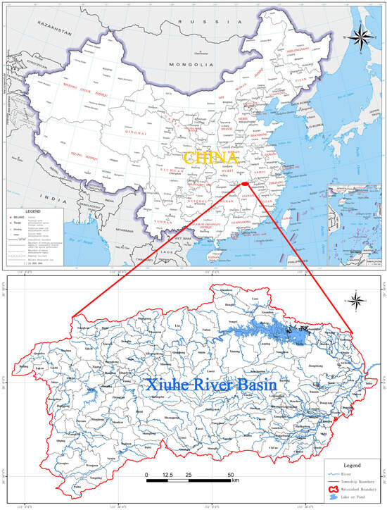
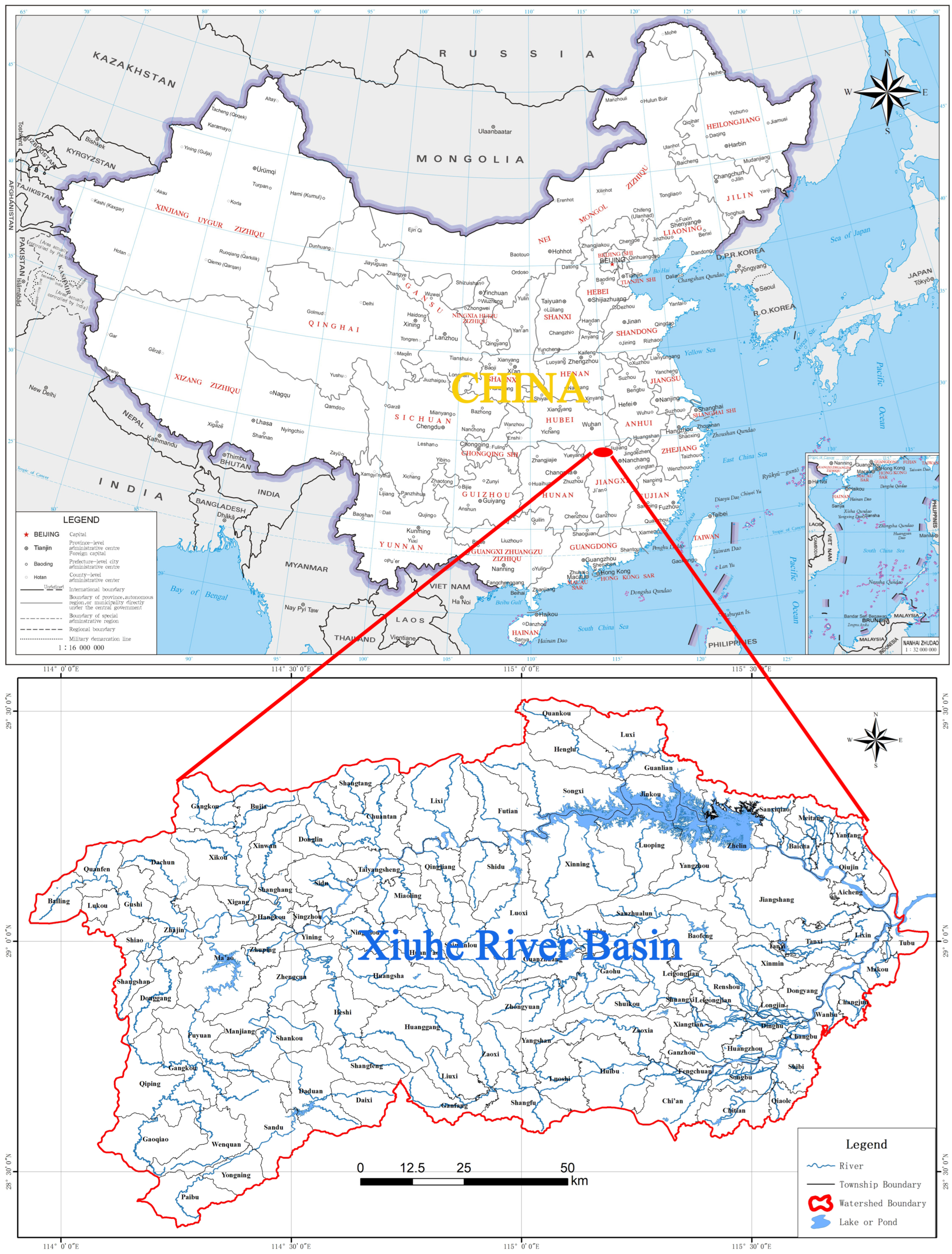
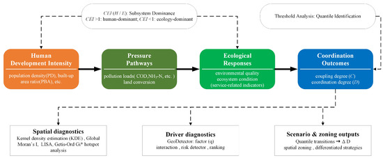
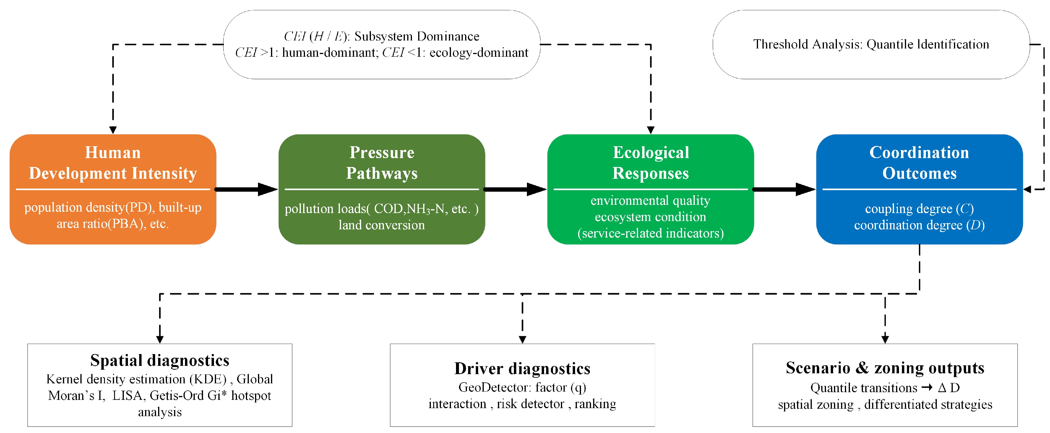
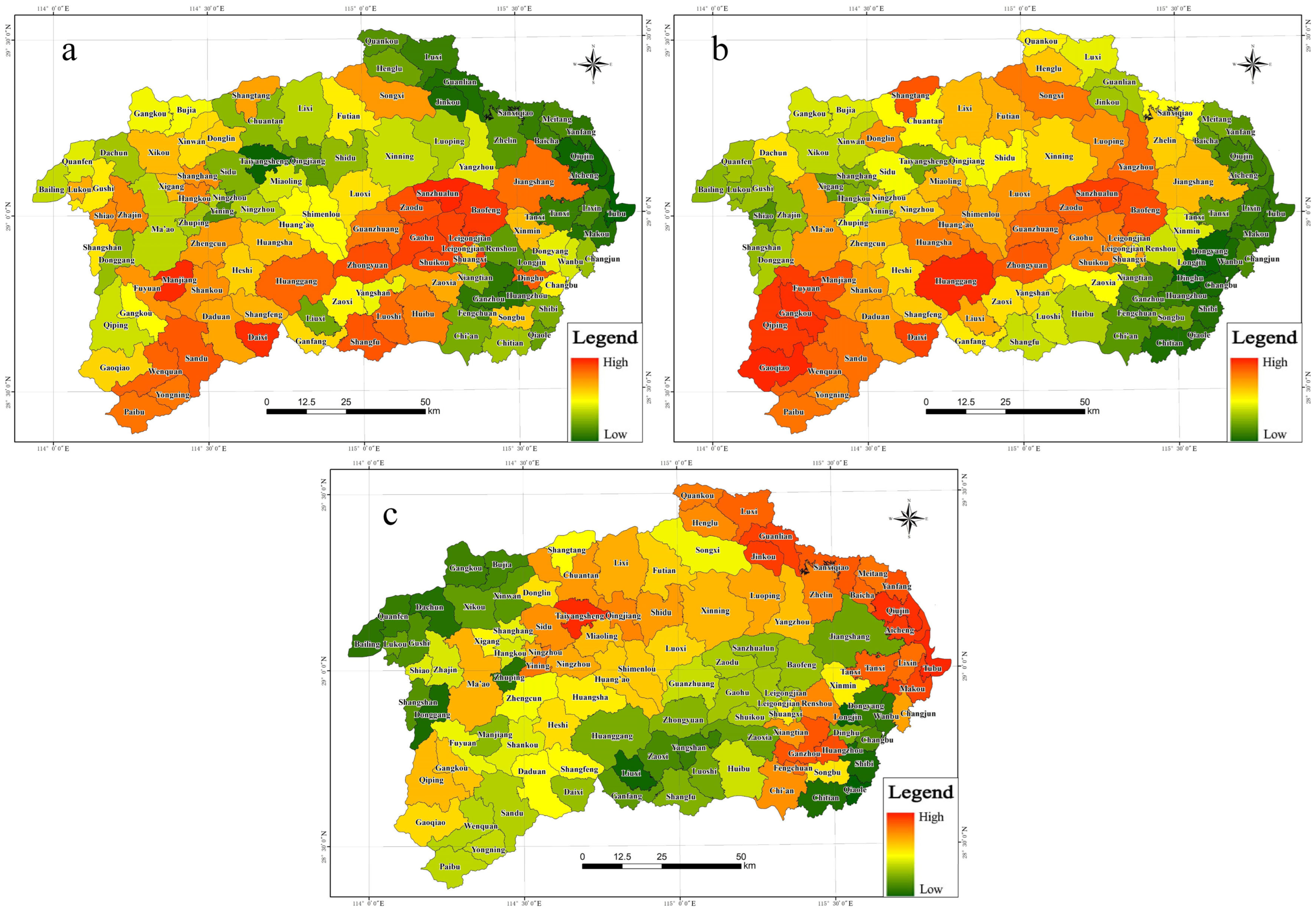
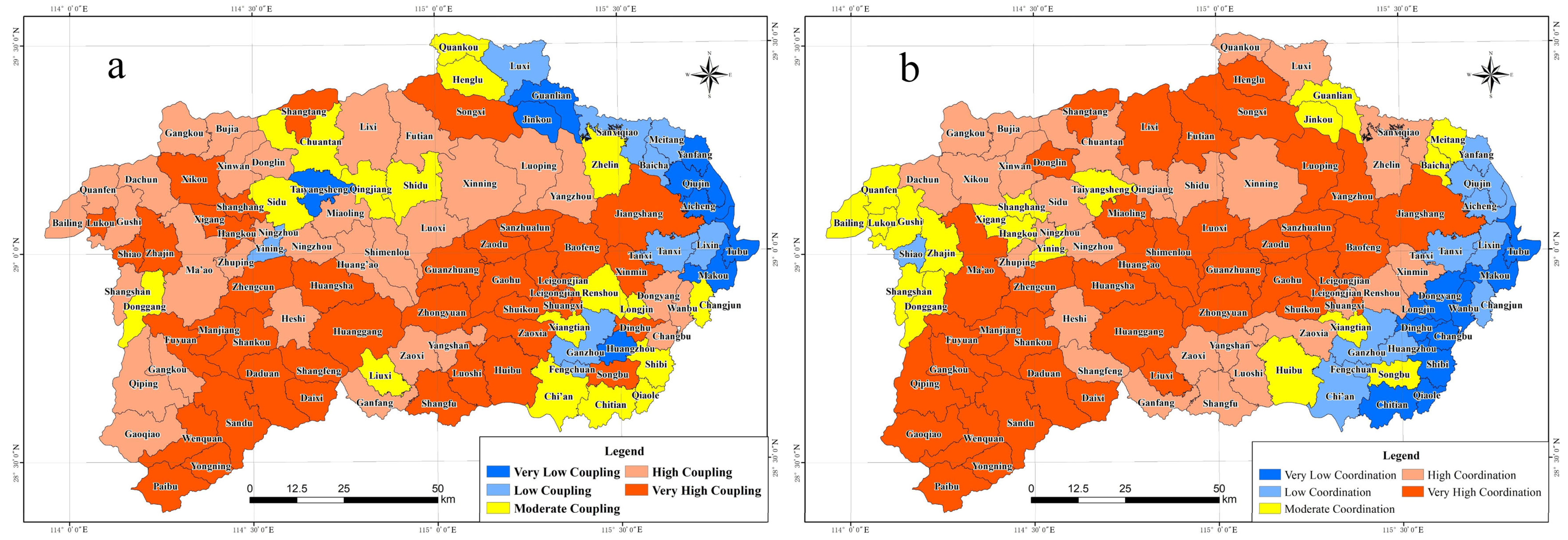
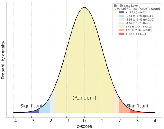
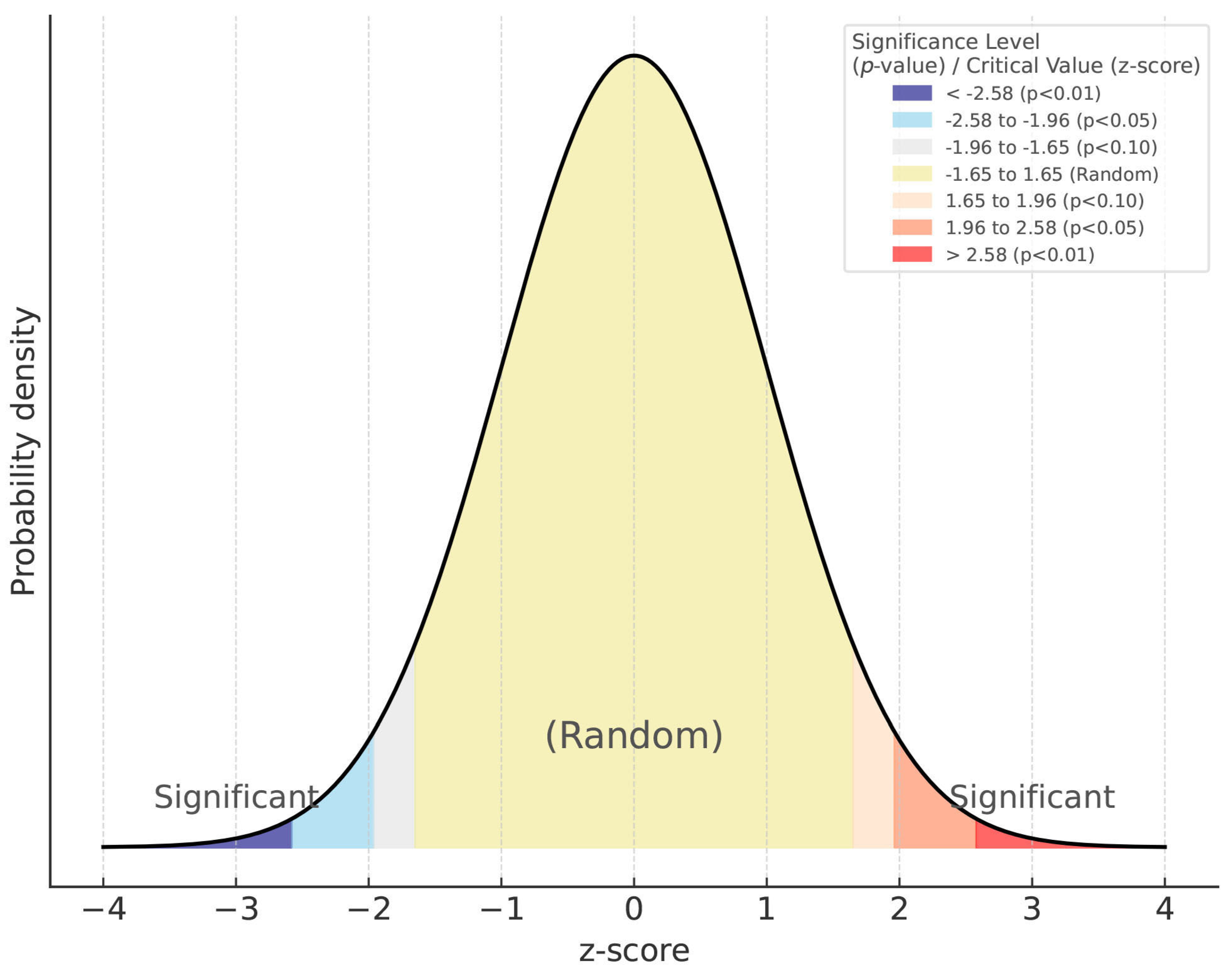
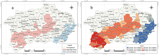
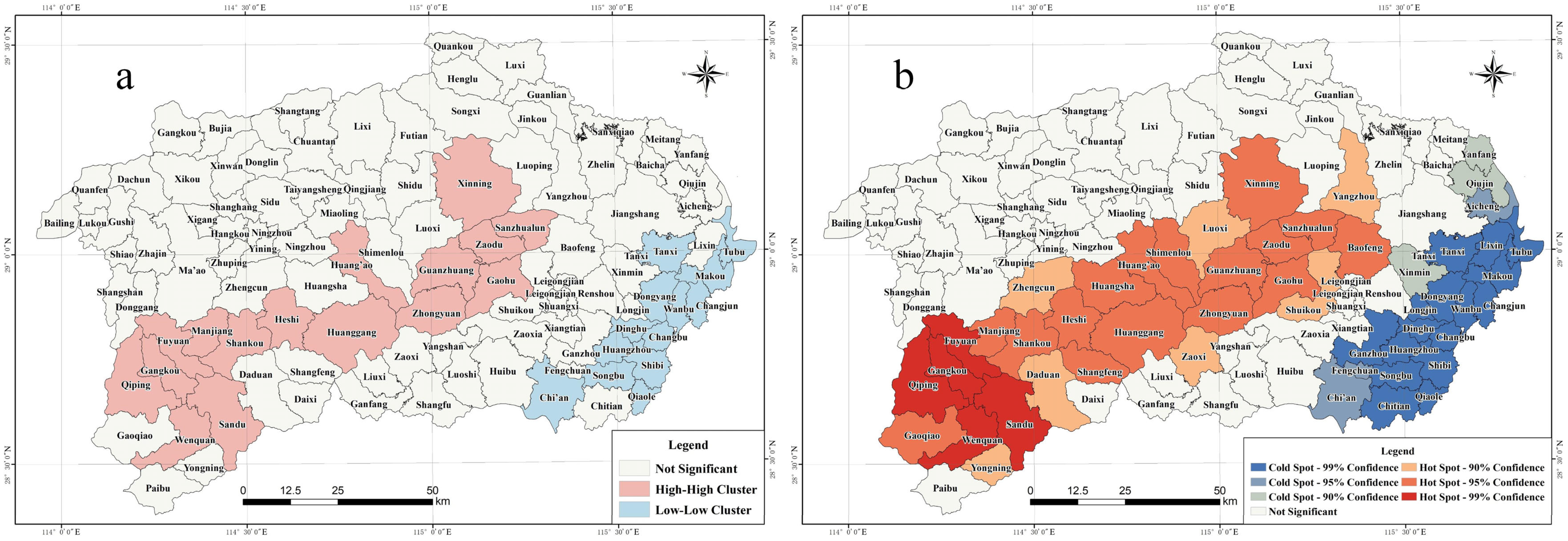
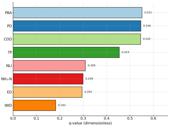
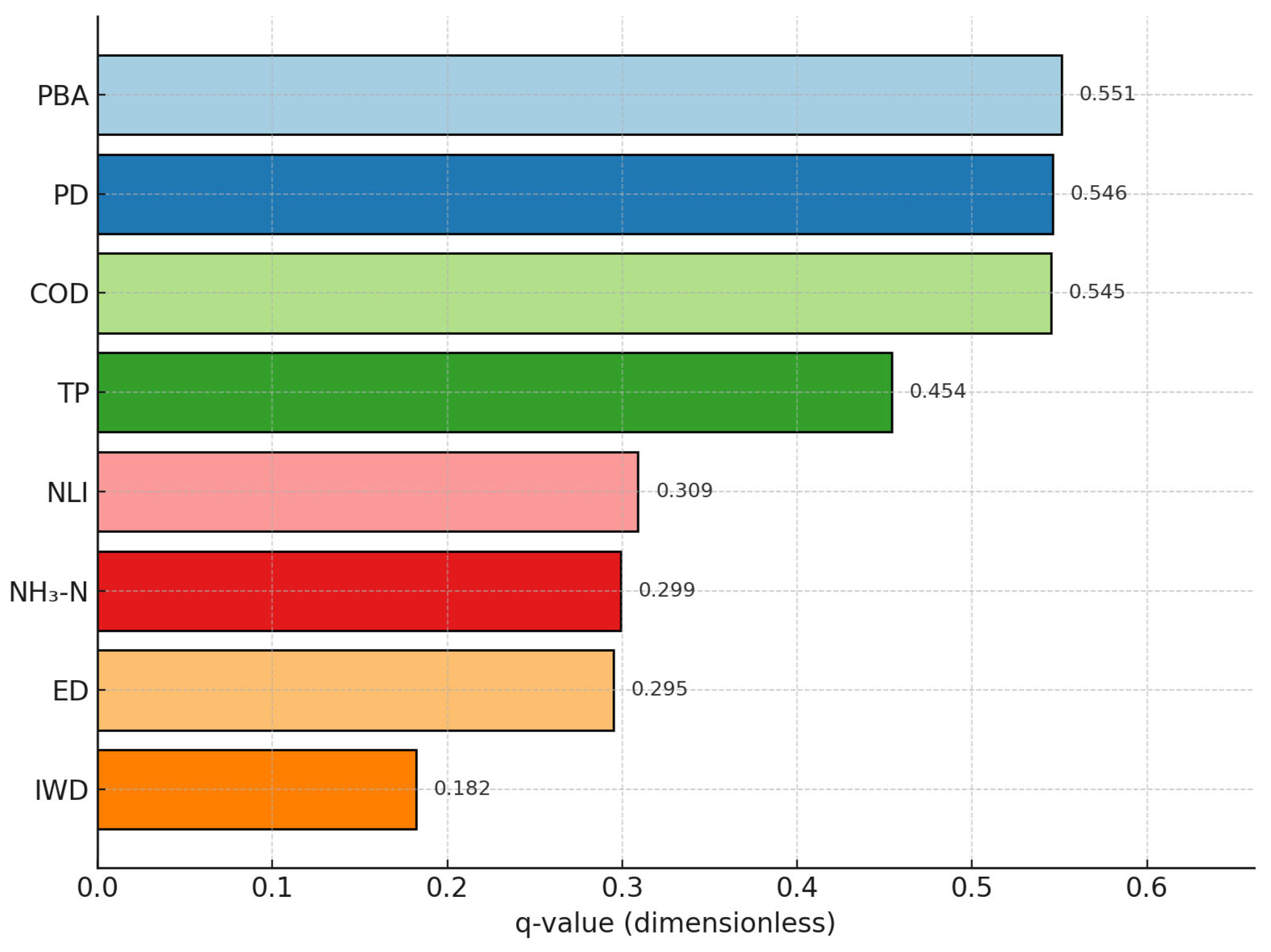
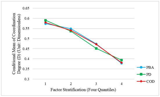
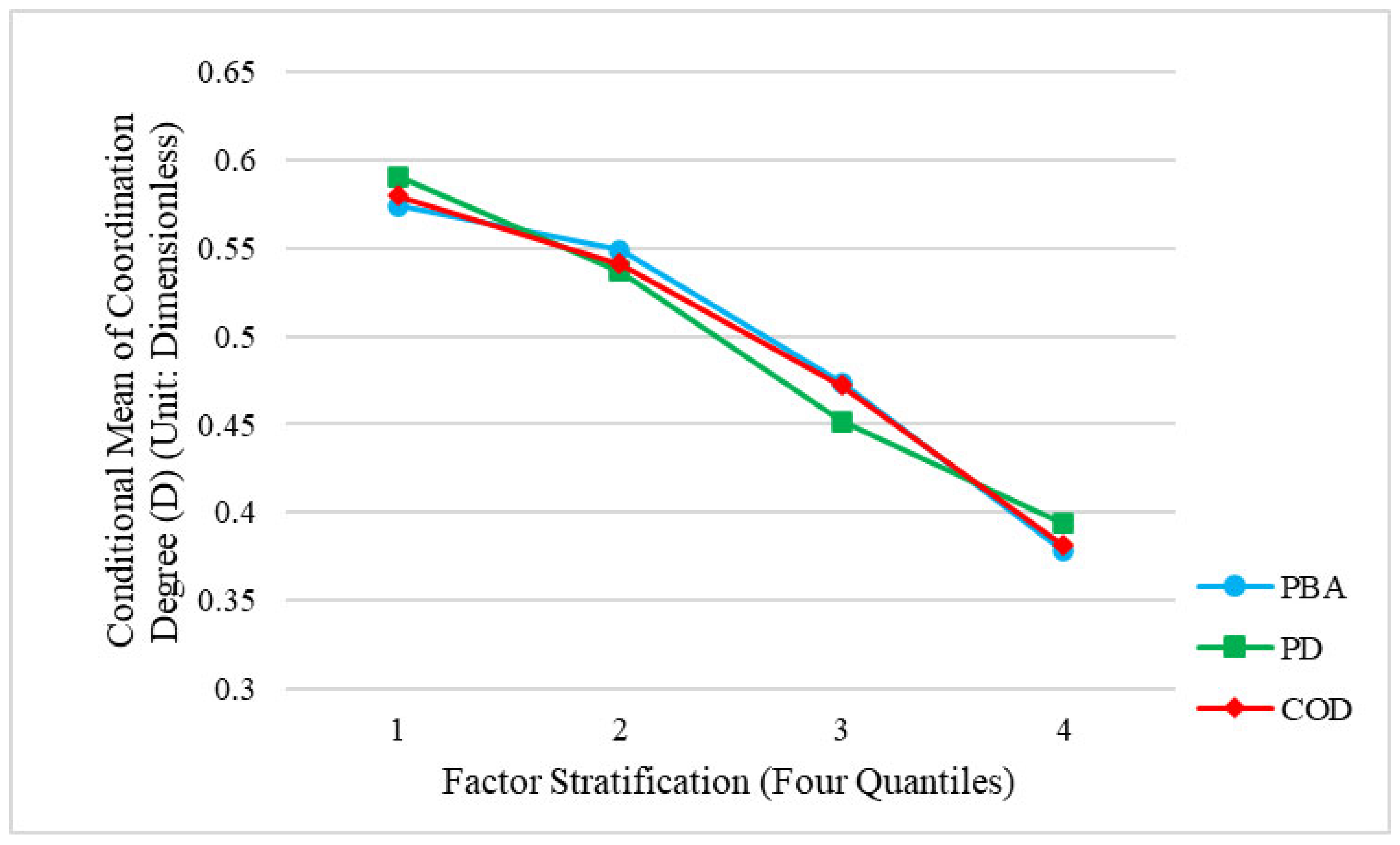
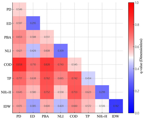
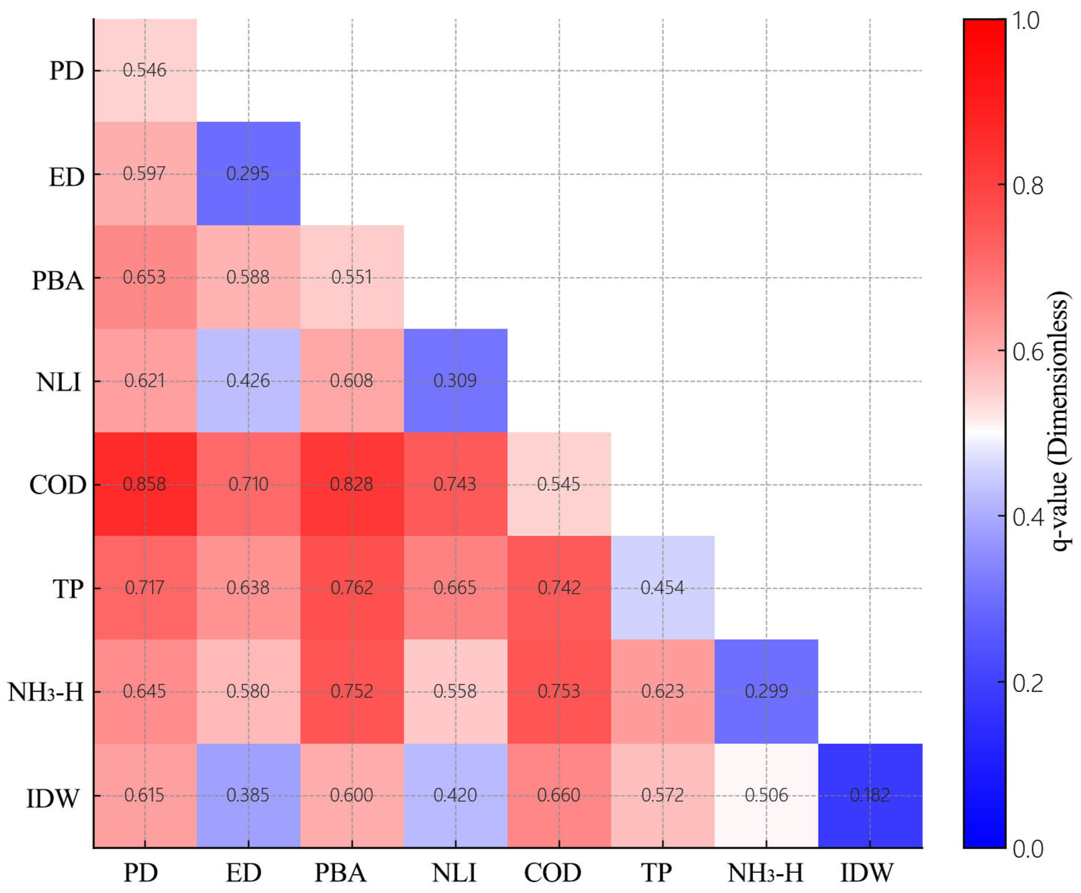

Disclaimer/Publisher’s Note: The statements, opinions and data contained in all publications are solely those of the individual author(s) and contributor(s) and not of MDPI and/or the editor(s). MDPI and/or the editor(s) disclaim responsibility for any injury to people or property resulting from any ideas, methods, instructions or products referred to in the content. |
© 2026 by the authors. Licensee MDPI, Basel, Switzerland. This article is an open access article distributed under the terms and conditions of the Creative Commons Attribution (CC BY) license.