


Abstract
Urban–rural transformation has increased the need to coordinate land use, settlement morphology, and heritage conservation at the edges of peri-urban traditional villages. This study examines 60 peri-urban traditional villages in Chaoshan, China, including 15 grid, 15 comb-shaped, 15 radial, and 15 mixed villages, using boundary-construction spans of 12, 30, and 100 m and four morphological indicators: aspect ratio (λ), weighted shape index (Sq), dispersion (σ), and saturation (θ). Statistical tests, exploratory clustering, machine-learning classification, nested cross-validation, and held-out SHAP interpretation were applied to examine morphological differentiation and its implications for land-use governance. All four indicators differed significantly among the morphology types (p < 0.001), with aspect ratio showing the largest effect (η2 = 0.588). Grid villages exhibited relatively regular edge configurations, comb-shaped villages showed strong elongation (λ = 2.447 ± 0.536), radial villages presented higher dispersion, and mixed villages showed the greatest boundary complexity and heterogeneity (Sq = 2.794 ± 0.902). These morphological differences highlight distinct spatial relationships involving settlement boundaries, axial connections, and core–edge organization. With Sq normalization estimated within training partitions, six classifiers achieved nested Macro-F1 values of 0.595–0.697, while the inner-selected system reached 0.687; SHAP identified aspect ratio as the strongest classification contributor. Grouped P25–P75 comparisons based on Sq, σ, and θ yielded 16, 13, 24, and 7 villages with zero to three out-of-band indicators, respectively, reflecting sample-relative morphological departures rather than verified ecological or heritage risks. From a landscape-ecology perspective, these findings support contextual examination of potential edge effects, corridor continuity, and surrounding land-use relationships. Together with four documented village cases, the study provides a comparative geometric basis for differentiated land-use governance and heritage conservation review, while the effectiveness of specific interventions requires independent field and planning evidence.
1. Introduction
1.1. Research Background and Problem Statement
Traditional villages preserve cultural heritage through buildings, streets, ancestral halls, and their relationships with water, public space, and productive landscapes. Conservation consequently extends beyond individual structures to settlement settings [1,2,3,4]. Urban–rural transformation has brought road expansion, residential construction, tourism development, and land conversion into these settings [5,6,7,8,9]. Village edges are a useful focus because they connect inherited settlement form with surrounding land uses. A practical assessment must distinguish geometric description from evidence that a particular interface experiences a conservation, access, or ecological problem. In the selected peri-urban villages, this transition setting is a defining locational characteristic: inherited settlement fabrics meet contemporary construction, infrastructure, and surrounding rural land uses. This makes the village–land interface particularly relevant to coordinated heritage conservation and land-use governance.
Landscape ecology directs attention to these interfaces through edge effects and the patch–corridor–matrix framework [10,11,12,13,14,15,16,17,18,19,20,21]. Buildings, roads, water, vegetation, and farmland meet at village margins, but geometry alone does not measure the function of their relationships. An irregular boundary may accommodate water or terrain; a regular one may coexist with discontinuous access. The relevant question is how measurable form can organize contextual investigation without being interpreted as ecological performance. Chaoshan contains contrasting village forms within a shared cultural region. Its historic buildings, streets, clan institutions, and water systems occupy plains, coastal areas, hills, and transitional terrains [1,22,23]. Previous work relates their configurations to production, transport, lineage organization, and construction practices [1,22,23,24,25,26,27,28,29,30,31]. This study compares four predefined types: grid, organized by repeated street–block relations; comb-shaped, with a dominant axis and lateral branches; radial, with a central node and outward connections; and mixed, combining several spatial organizations.
Descriptions of peripheral construction, axial interfaces, center–periphery relations, and overlapping development pressures motivate comparison of these forms [32]. A type-sensitive geometric baseline can organize review of such interfaces, while identifying an actual land-use or heritage problem requires contextual evidence. A single geometric standard would obscure characteristic differences. Elongation may be expected in a comb-shaped village. Area-ratio differences require comparison with mapped water, farmland, and open space; θ alone does not identify their presence. Indicator-dependent reference groups describe shared numerical patterns while retaining the four village types; their use in governance depends on verification of the surrounding land and current planning context. Section 1.2 reviews the relevant landscape-ecological and methodological literature, while Section 1.3 sets out the research questions, objectives, and contributions.
1.2. Literature Review
1.2.1. Traditional-Village Morphology and Edge-Space Research
Landscape ecology links spatial patterns with processes while emphasizing the influence of observational scale. Forman and Godron’s patch–corridor–matrix framework explains the organization of landscape elements [17,18]; Turner distinguishes spatial pattern from the processes it may influence [19]; and Levin demonstrates the dependence of pattern interpretation on scale [20]. Connectivity provides a further basis for examining relationships among spatial units [21]. For traditional villages, these perspectives extend conservation analysis beyond buildings and streets to the connections among settlement cores, water systems, open spaces, and surrounding land. Village edges are particularly relevant because several of these elements meet within a relatively limited area.
Quantitative landscape research also shows why multiple indicators are needed. FRAGSTATS and related approaches describe complementary dimensions of shape, area, boundary complexity, and configuration [33,34,35], while studies of scale demonstrate that the apparent structure of a spatial object can change with the analytical extent or resolution [36,37]. Village-edge analysis should therefore consider directionality, boundary complexity, cross-scale variation, and relative enclosed area together. These dimensions provide structural descriptions whose landscape meaning depends on the context in which they occur. Traditional-village research has increasingly used GIS, spatial statistics, GeoDetector, and machine learning to investigate regional clustering and associated factors [1,22,38,39,40,41]. Studies of spatial typologies, spatial genes, street networks, parametric reconstruction, and settlement evolution have also advanced the analysis of village form [23,24,25,26,27,28,29,30,31,42]. Much of this work addresses either the distribution of whole settlements or their internal organization. It provides a basis for comparative analysis but leaves the interface between settlement form and surrounding land less fully resolved. Research on physical and virtual boundaries has begun to address this interface through flexible conservation extents and multiple analytical scales [25,43,44,45,46]. These approaches distinguish settlement cores, transition zones, and broader landscape settings instead of relying on a single fixed outline. They also provide a basis for comparing how local building configurations relate to more extensive settlement envelopes.
1.2.2. Multi-Scale Morphological Quantification
Analytical boundary spans of 12, 30, and 100 m describe local, intermediate, and broader village-edge configurations. Earlier studies used different distance combinations according to settlement form and purpose [43,44,45,46]. These values follow the virtual-boundary-construction approach of Nie et al. [25] and its subsequent application by Zhang and Yang [47]. Here, they are fixed maximum connection spans rather than uniform outward-buffer widths. Their suitability is not established against every alternative, and transfer to other regions requires local assessment.
Four indicators describe complementary aspects of the resulting geometry. Aspect ratio (λ) measures envelope directionality and elongation; weighted shape index (Sq) describes boundary complexity across scales; dispersion (σ) expresses the contrast in boundary complexity between local and broader scales; and saturation (θ) measures the large-scale enclosed area relative to the orientation-search rectangle derived from building geometry. Rhino and Grasshopper support consistent boundary construction and indicator calculation across villages. As in other landscape-metric approaches, these indicators describe spatial structure rather than directly measuring ecological functions [33,34,35,36,37]. Higher complexity or greater cross-scale contrast may warrant examination, but their interpretation requires information about roads, water, open spaces, land use, and observed building patterns.
Alongside geometric measurement, recent studies have applied machine-learning methods to identify settlement or neighbourhood types and examine the development potential of traditional villages [48,49]. These applications also highlight the importance of robust model evaluation, including controlling model-selection bias and data leakage, addressing limited sample sizes, and interpreting model predictions [50,51,52,53].P25–P75 intervals describe the central portion of a selected reference distribution [54]. Retaining the archived comparative grouping, some morphologies share a reference set for a given indicator. The grouping and percentile rule therefore affect which villages fall outside the interval. Tail positions are expected and do not identify undesirable conditions; sample size, shared indicator information, and landscape context constrain their interpretation [54,55,56].
1.2.3. Explainable Machine Learning in Village Morphology Research
Village plans can overlap across predefined morphology types, making visual assignment difficult in some cases. This motivates exploration of whether four reproducible geometric indicators can provide an initial, interpretable type suggestion for newly examined traditional villages, consistent with the broader use of spatial features for supervised settlement classification [48]. In this study, machine learning evaluates the recovery of labels assigned from complete village plans within a fixed 60-village dataset. Because the labels and indicators describe related aspects of the same settlement form, this is an internal geometric consistency and classification-feasibility test, not independent validation of the typology, regional representativeness, land-use problems, or predictive performance for unseen villages. Related applications of interpretable classification provide additional methodological context [49]. Repeated nested cross-validation separates classifier-family and hyperparameter selection from outer-fold label evaluation [50]. Preprocessing parameters must also be estimated within each training partition to prevent information from held-out feature distributions entering model construction [51]. This study therefore constructs Sq separately within the inner and outer training folds. Such separation supports internal evaluation with limited samples [52], but does not make geometrically related labels and features independent or establish performance in new regions.
SHAP-based interpretation then describes the contribution of each indicator to model outputs [53]. The analysis examines both overall feature importance and differences among morphology classes, allowing classification evidence to be compared with descriptive and statistical findings. Attribution remains specific to the fitted model and its predictions. It cannot establish that an indicator causes settlement formation, land-use change, or ecological outcomes; these processes require separate evidence. Accordingly, SHAP supports interpretation of the classification test without extending its conclusions to causal mechanisms.
1.2.4. Research Gaps
Despite increasing research on traditional-village conservation and settlement morphology, several gaps remain. First, previous studies have mainly focused on the spatial distribution, historical development, and internal organization of traditional villages [1,22,23,24,25,26,27,28,29,30,31,42]. Less attention has been paid to village-edge spaces, where historic settlements interact with surrounding roads, farmland, water systems, and new construction. A systematic understanding of these spatial interfaces is important for coordinating heritage conservation and land-use management. Second, existing morphological studies have demonstrated the value of landscape metrics and multi-scale spatial analysis [25,33,34,35,36,37,43,44,45,46,47]. However, different village types have distinct geometric characteristics, and applying uniform evaluation standards may overlook these differences. Comparative approaches that consider both settlement types and spatial scales are therefore needed. Morphological indicators should also be interpreted as descriptions of spatial form rather than direct measures of ecological quality or heritage condition.
Additionally, machine learning and explainable methods have been increasingly applied to settlement research [38,39,40,41,48,49,50,51,52,53]. Although these approaches can reveal relationships between morphological indicators and predefined village types, their classification results do not necessarily provide independent validation. Similarly, SHAP explanations indicate model contributions rather than causal relationships. Transparent validation and careful interpretation are therefore essential. Finally, the relationship between morphological analysis and practical land-use governance requires further attention. Quantitative indicators alone cannot confirm specific conservation problems or planning conflicts. Their interpretation should be combined with village plans, field observations, and relevant planning documents. Accordingly, this study integrates multi-scale morphological analysis, machine learning–SHAP interpretation, and documented village cases to provide a comparative geometric basis for differentiated heritage conservation and land-use governance review.
1.3. Research Questions, Objectives, and Contributions
The analysis uses 60 peri-urban traditional villages selected from a regional inventory described as containing more than 110 candidates. Peri-urban location was a substantive selection criterion, alongside data availability, plan legibility, and fixed quotas of 15 villages per type to support balanced comparison. The design does not estimate regional type prevalence. Figure 1 presents the regional inventory context and the spatial distribution of the selected sample. The available archive does not preserve a complete candidate-by-candidate exclusion ledger. The research problem is how to use comparable, type-sensitive geometry to organize review of village-edge spaces without mistaking geometric differences for verified heritage or ecological impacts. This study aims to quantify morphological differences among predefined village types, examine the internal consistency and feasibility of indicator-assisted preliminary type identification, and identify conditional questions for site-specific land-use and conservation review. Its contribution is a transparent comparative baseline and evidence-aware review process, not a tested spatial optimizer or a causal explanation of settlement transformation.
Figure 1.
Study area and regional reference locations of the 60 sampled traditional villages by morphological type in Chaoshan, China. The analytical sample comprises 15 grid, 15 comb-shaped, 15 radial, and 15 mixed villages, identified by color and symbol. Gray markers retain the background source inventory and do not designate additional analytical samples.
The study addresses three research questions:
RQ1: How do the four indicators differ among the selected village types, and what positions do individual villages occupy relative to the indicator-dependent empirical reference groups?
RQ2: To what extent can four quantitative indicators support exploratory machine-learning-assisted identification of predefined morphology types within the selected sample, and which features contribute to the fitted classification probabilities?
RQ3: Which contextual review questions can these geometric descriptions suggest for land-use governance, and what additional evidence is required before action?
The contribution combines a multi-scale geometric baseline, comparisons among preassigned types, internal label consistency, and direction-preserving records of individual variation. RQ1 and RQ2 are tested with the measured sample; RQ3 uses archived cases to formulate contextual governance questions. This structure links the quantitative results to a documented review process without claiming evaluated intervention outcomes. The analysis is cross-sectional. Present-day geometry cannot reconstruct complete settlement histories or directly establish ecological function, resilience, or cultural continuity. Landscape ecology provides an interpretive framework, and heritage conservation defines the governance context. Explanations of observed departures and assessments of intervention outcomes require field investigation and, where change is concerned, multi-temporal evidence. These limits guide the use of classification and deviation results throughout the study.
Figure 2 distinguishes the measured analyses from contextual interpretation. Archived geometry supports the indicators, statistical comparisons, and reference-band positions. Nested classifier selection uses Sq constants estimated only from the corresponding training observations, and SHAP explains outer-test label probabilities. The full-sample descriptive Sq is retained separately for morphological comparisons. Archived case context suggests questions for field and planning review; it does not validate interventions.
Figure 2.
Research framework linking spatial archives, multi-scale geometry, sample comparisons, internal label consistency, and conditional land-use review. The original spatial diagrams and analytical insets are schematic; inset charts do not report additional numerical results. Boundary distances are connectivity-span settings. The implemented definitions, training-partition Sq construction, and validation design are detailed in Section 2. Ecological, heritage, and governance outcomes require separate evidence.
2. Materials and Methods
2.1. Study Area and Sample Selection
Chaoshan, comprising Shantou, Chaozhou, and Jieyang in eastern Guangdong, China, encompasses plains, coastal settlements, hilly terrain, and water-linked landscapes. These contrasting settings provide a basis for comparing village-plan configurations and edge-space morphology.
All 60 retained villages were selected in peri-urban transition settings, where inherited village fabrics interface with contemporary development, infrastructure, and surrounding rural land uses. In this study, peri-urban is used as a qualitative locational and sampling characteristic rather than a statutory planning-zone designation or a uniform distance band from an urban boundary. The original selection considered this urban–rural interface together with heritage relevance, settlement-morphology diversity, and the availability of interpretable spatial materials. The four morphological indicators quantify the selected villages’ geometric configurations; they are not used to establish peri-urban status or measure the intensity of urbanization.
The initial candidate inventory comprised more than 110 villages, primarily including locally recognized traditional settlements and villages associated with Guangdong’s Baiqianwan initiative for high-quality development of counties, towns, and villages. The candidates were manually reviewed, with attention to their heritage or local-development context, the diversity of terrain settings and settlement forms, the availability of usable spatial materials, and the legibility of building and village-plan configurations. Before the final selection of 60 villages, the 12, 30, and 100 m virtual-boundary connection spans were applied to more than 110 candidate villages across different terrain and settlement configurations in Chaoshan. This preliminary application was used to assess the practical feasibility of constructing interpretable multi-scale boundaries and informed the subsequent purposive, balanced sample selection. It was not a systematic comparison of alternative span combinations or an independent test of transferability outside Chaoshan. From this inventory, 60 villages were retained as a purposively balanced comparative sample, with 15 cases in each of four predefined morphology groups: grid, comb-shaped, radial, and mixed. Equal group sizes were chosen to facilitate between-type comparisons and classifier assessment without allowing a numerically larger group to dominate the sample. The selection therefore emphasizes geographic-setting and morphological diversity for comparative analysis rather than probability-based regional representativeness; neither the sample proportions nor the classification results estimate the prevalence of these types across all villages in Chaoshan.
Table 1 summarizes the reported data families and their intended analytical roles. The retained archive includes village-level workbooks, 60 Rhino sample models, the Grasshopper definition, and boundary drawings; it does not preserve a complete source and verification record for every reported data family. Inspection recovered coordinate-reference tags from 33 of 35 TIFF files, including figure exports and duplicate case imagery. These files do not constitute a complete 60-village metadata inventory. Per-village acquisition dates, positional-accuracy estimates, and georeferencing histories remain incomplete. Recovered metadata records are retained in the project archive and may be requested from the corresponding author, subject to availability, applicable permissions, and confidentiality requirements.
Table 1.
Data types, formats, sources, and analytical roles.
All 60 archived Rhino sample models specify meters and an absolute geometry tolerance of 0.01 m. No dedicated surveying instruments or laboratory equipment were used to generate new measurements in this study. Instead, the analysis relied on existing spatial materials, including Google Maps remote-sensing imagery, village spatial plans, GIS vector datasets, DWG drawings, and archived field-survey records collected during 2022–2025. These settings describe the modelling environment, not imagery positional accuracy. Small-boundary construction used 12 m. Legacy layer names referring to 7 m reflect earlier working terminology and do not represent the final construction span; the retained workflow uses 12 m. The layer names alone are not records of the preliminary trials. The archived definition contains the 12, 30, and 100 m settings. Its saved state documents the calculation protocol, although a complete execution and manual-edit log for each village is unavailable. Spatial data were projected to meter-based coordinates in ArcGIS Pro 3.2 (Esri, Redlands, CA, USA)before import into Rhino and Grasshopper for boundary construction and indicator calculation. Labels were assigned from the complete plan configuration before indicator calculation. Grid required repeated orthogonal or near-orthogonal street–block relations; comb-shaped had a dominant spine with lateral branches; radial had a recognizable center and outward organization; and mixed had overlapping structures without one dominant whole-settlement logic. Table 2 defines the groups, and Figure 3 and Figure 4 illustrate plan and boundary interpretation. Because the indicators summarize related geometry, differences among these selected groups are partly expected. No inter-rater agreement statistic is available.
Table 2.
Preassigned morphology groups, classification criteria, representative spatial form, and sample size.
Figure 3.
Workflow for traditional-village morphology interpretation and multi-scale edge-space construction. Step 1 presents representative grid, comb-shaped, radial, and mixed morphologies; Step 2 illustrates the interpretation of buildings, roads, water, vegetation, farmland, and the village boundary from remote sensing; Step 3 relates plan form to the village boundary and minimum bounding rectangle; and Step 4 shows base-boundary extraction, the 12, 30, and 100 m analytical boundaries, and the corresponding edge-space zones. Representative cases illustrate the workflow and are not used as independent ecological evidence. In Step 4, the boundary bands are schematic and not to scale; the distance labels denote virtual-boundary span settings, not uniform outward-buffer widths.
Figure 4.
Representative settlement-morphology cases and boundary interpretation. Panel (A) presents four comparative town configurations and Panel (B) four representative village configurations. Black indicates building footprints, red the analysis or village boundary, and green the morphology-derived edge boundary; background colors show surrounding built-up land, green space, water, and agricultural land. The town cases serve only as comparative references for boundary interpretation and are not included in the 60-village statistical or machine-learning sample.
2.2. Morphology Types and Multi-Scale Boundary Delineation
Grid villages are organized by intersecting streets and repeated blocks; comb-shaped villages combine a dominant axis with lateral branches; radial villages organize routes and building groups around a central node; and mixed villages combine several organizational logics in response to terrain, water, roads, lineage growth, or later construction. These types establish different expectations for elongation, compactness, dispersion, and relative area. Figure 4 juxtaposes comparative town configurations and representative village configurations to clarify the distinction between the analysis boundary and the morphology-derived edge boundary. The town panels are interpretive references only and are not members of the 60-village statistical or machine-learning sample.
Building outlines and available road, water, vegetation, and open-space layers were digitized and checked before Rhino–Grasshopper calculation. Physical boundary segments followed mapped edges; the boundary definition also joined components where a closed envelope was required. The archived curve-cleaning and boundary-generation controls contain a 1 m automatic-gap-closure setting, a small-area cleanup setting of 1 m2, and an angular simplification setting of 1°. The archived connection trace is retained in the project archive and may be requested from the corresponding author, subject to availability and applicable source-data and project permissions. During boundary delineation, a second researcher independently reviewed a subset of village boundaries and the corresponding measurements. The reviewed cases showed relatively small discrepancies, providing preliminary support for consistency within the checked subset. These checks were not a comprehensive inter-observer reliability study or a quantified uncertainty assessment of all 60 villages. A formally documented paired comparison and a complete manual-adjudication ledger are unavailable.
The analytical boundary settings are S1 = 12 m, S2 = 30 m, and S3 = 100 m. In the retained definition, these controls are labeled Border span(m) and specify maximum virtual-boundary connection spans; the edge zones between the resulting curves are not uniform-width outward buffers. The scale combination follows published traditional-village applications [25,47]. During preliminary boundary-construction trials, a 7 m small-scale span was also attempted, but was too short to provide a satisfactory boundary representation for some village layouts. This was exploratory work, not a systematic sensitivity experiment across all 60 villages. The retained spans were applied consistently to enable comparison of local, intermediate, and broader configurations. Figure 5 illustrates these relationships conceptually. The settings are not optimized site thresholds or statutory setbacks, and their applicability remains conditional on local mapping and settlement context.
Figure 5.
Conceptual framework of multi-scale village-edge spaces and potential landscape interactions. Yellow, blue, and red boundaries represent S1 (12 m), S2 (30 m), and S3 (100 m), respectively. The labels denote boundary-construction spans, not uniform outward-buffer widths. Inner and outer edge spaces relate immediate built interfaces to the surrounding landscape; arrows indicate potential interactions for field review. The schematic bands are not to scale.
Figure 6 illustrates the application of this framework in Jizhen Village. The mapped boundaries distinguish the inner edge space between S1 and S2 from the outer edge space between S2 and S3. The inner edge captures the immediate relationship between buildings and adjacent open spaces, while the outer edge places these local interfaces within a broader surrounding envelope. Their extent follows the mapped settlement configuration, including irregular margins and discontinuities. The three boundaries provide the geometry for the four indicators defined in Table 3. Figure 7 documents the GIS–Rhino–Grasshopper construction and calculation sequence, and Figure 8 relates mapped spatial elements to the landscape context.
Figure 6.
Delineation of multi-scale village-edge spaces in Jizhen Village. Yellow, blue, and red dotted lines indicate the small (S1 = 12 m), medium (S2 = 30 m), and large (S3 = 100 m) boundaries, respectively. Gray denotes village buildings and white denotes the village interior; dark teal and light cyan distinguish the inner edge space (S1–S2) and outer edge space (S2–S3). The distance labels denote boundary-construction spans; the intervening zones follow the settlement geometry and are not uniform-width outward buffers.
Table 3.
Operational definitions and analytical dimensions of the four village-edge morphology indicators.
Figure 7.
GIS–Rhino–Grasshopper workflow for multi-scale village-edge construction and indicator calculation. Satellite imagery, field measurements, and planning CAD layers were digitized and reconstructed in Rhino, while Grasshopper generated analytical boundaries using connectivity spans of 12, 30, and 100 m and exported the four morphological indicators. Original model and node screenshots are retained; the export inset identifies fields rather than unaudited demonstration values. A denotes the orientation-search reference rectangle derived from building-outline geometry, and θ = A3/A. Plus signs indicate data integration, while arrows show the workflow from spatial-element extraction and digitization to Grasshopper processing. Different colors represent buildings, roads, plazas, vegetation, and water, while red outlines indicate village boundaries.
Figure 8.
Patch–corridor–matrix interpretation of a traditional-village edge. Settlement and heritage spaces interact with road, water, drainage, view and ecological corridors and with surrounding farmland, woodland and peri-urban construction. The diagram organizes field questions rather than asserting measured ecological functions.
2.3. Landscape Morphology Indicators
Village-edge morphology is multidimensional, and no single measure can represent direction, boundary form, cross-scale contrast, and relative enclosed area at once. The analysis therefore separates four complementary questions: whether the edge has a dominant direction; how complex its boundary is across scales; how strongly local boundary complexity differs from the broader envelope; and how the S3 enclosed area compares with a rectangle fitted to building-outline geometry. This separation follows settlement-boundary quantification and landscape-metric research emphasizing metric specificity and scale dependence [33,34,35,36,37,43,44].
Aspect ratio (λ), weighted shape index (Sq), dispersion (σ), and saturation (θ) correspond to those four dimensions. They are morphological descriptors rather than direct ecological-performance measures: λ records overall directionality or elongation; Sq records multi-scale boundary complexity; σ records local-to-broad boundary-complexity contrast; and θ records the ratio of S3 enclosed area to the orientation-search rectangle area fitted to building-outline geometry. To distinguish the boundary labels S1–S3 from their calculated shape metrics, SIi denotes the scale-specific shape-index value at scale i. Table 3 consolidates the definitions, expressions, analytical dimensions, and interpretive limits.
Table 3 gives the operational definitions. For λ, x and y are the long and short sides (x ≥ y) of a village-specific orientation-search rectangle. The archived Grasshopper connections pass a mesh of building-outline vertices to the rectangle component, use a direction-search count control set to 1000, and retain the smallest tested area. Both λ and rectangle area A come from that selected geometry; A3 is supplied separately by the S3 boundary-area component. Thus, θ = A3/A uses the S3 area and the building-geometry rectangle, rather than a separately fitted S3 rectangle. The two geometries have different inputs; θ is a comparative area ratio, not a geometric coverage fraction. Values below one do not establish that the S3 boundary lies inside the building-based rectangle. Orientation is not fixed to common map axes; the saved Dongpan example is rotated by approximately 0.569°. This is an orientation-search approximation, not a proof of exact global optimality. Pi and Ai are the perimeter and enclosed area at each boundary scale, and SIi is its shape index. The fixed descriptive Sq retains μ1 = 3.944897, μ2 = 2.158947, and μ3 = 1.416515 for complete-sample comparisons and reference bands. For machine-learning evaluation, the same formula and weights use means estimated only from each training partition; those means are applied unchanged to its held-out observations.
Formula verification reproduced every Sq value within 3.29 × 10⁻⁷ and every θ value within archived export precision. The retained σ series was calculated directly as SI1/SI3 from the recorded numerical inputs. The workbook-derived A3 field supports an algebraic consistency check rather than independent verification of source polygons. Figure 7 records the boundary-generation and indicator-calculation workflow.
2.4. Landscape-Ecology Interpretation and Statistical Analysis
Landscape ecology was applied after measurement as an interpretive framework. The patch–corridor–matrix model organized questions about building groups, ponds, groves, public spaces, routes, waterways, and the surrounding land matrix. Figure 8 visualizes this relational reading: settlement and heritage spaces interact with road, water, drainage, view, and ecological corridors and with the surrounding farmland, woodland, and peri-urban matrix. The diagram does not convert the village into an ecological habitat model; it identifies spatial relations that require field verification.
Edge-effect concepts focus attention on interfaces and possible disturbance exposure, while pattern–process reasoning formulates field questions and scale dependence separates local, intermediate, and broader observations. None of the four indicators was treated as a direct measure of habitat quality, hydrological function, ecological resilience, connectivity, or cultural value. Figure 2 summarizes the evidence chain, and Figure 8 supplies the spatial vocabulary used for contextual field review.
Mean-centered Levene tests determined the variance-sensitive comparison: Welch ANOVA with Games–Howell contrasts when p < 0.05, and one-way ANOVA with Tukey HSD otherwise. Omnibus η2 was calculated from conventional between-group and total sums of squares and reported descriptively alongside either test; its 95% interval used 5000 stratified bootstrap resamples with seed 20260913. One-dimensional K-means, fixed at k = 3 with 100 initializations and the same seed, is retained only as a compact exploratory summary. It neither assigns village types nor defines reference bands or governance categories. Spearman rank correlations among the four indicators were calculated across the 60 complete village records to describe pooled dependence; no feature was removed, or classifier refitted.
2.5. Grouped Empirical Reference Bands and Departure Review
Reference groups retain the indicator-dependent comparative structure of the archived study [32]. For λ, grid and radial share a reference set, while comb-shaped and mixed remain separate. For Sq, grid is separate, comb-shaped and radial are pooled, and mixed is separate. For σ and θ, grid is separate, and the other three types are pooled. These are descriptive comparison groups, not evidence of equivalent distributions. Nearest-rank P25 and P75 are the sorted observations at ranks ceiling(0.25n) and ceiling(0.75n). Comparisons use full precision and include both endpoints. The primary count sums out-of-band Sq, σ, and θ values (0–3); a separate four-indicator summary adds λ. Reference membership, departure directions, and both counts were computed using the method specified here; supporting calculation records may be requested from the corresponding author, subject to availability and applicable permissions.
Reference sets contain 15, 30, or 45 observations. With distinct values, the nearest-rank bands contain nine, 16, or 23 observations, respectively. Tail membership is expected, and a morphology within a pooled reference set need not have the same out-of-band proportion as another. Below- and above-band positions contribute equally to the count but suggest different contextual questions. Sq and σ share shape-index inputs and are not independent evidence dimensions. No ecological, heritage, or planning outcome calibrates the count. These sample-derived bands are not normative thresholds [54,55,56]; being outside P25–P75 also differs from the 1.5 × IQR boxplot-outlier rule. Interpretation requires departure direction and independent contextual evidence.
2.6. Multi-Model Classification and SHAP-Based Interpretation
Six model families were retained: multinomial logistic regression, sigmoid-calibrated RBF-SVM [57], Gaussian naive Bayes, KNN, XGBoost [58], and random forest [59]. Features were standardized inside the logistic, SVM, Gaussian NB, and KNN pipelines; tree models used unscaled inputs. Median imputation was included within each pipeline although the four analyzed columns contained no missing values. The examined grids were C ∈ {0.01, 0.03, 0.1, 0.3, 1, 3, 10} for logistic regression; C ∈ {0.1, 1, 10, 100} and γ ∈ {scale, 0.01, 0.1, 1.0} for RBF-SVM, with three-fold sigmoid calibration; variance smoothing ∈ {10−12, 10−11, …, 10−6} for Gaussian NB; k ∈ {3, 5, 7, 9, 11} with uniform or distance weights and Manhattan or Euclidean distance for KNN; 80 or 160 trees, depth 1–3, learning rate 0.03 or 0.1, subsample 0.8, and column subsample 1.0 for XGBoost; and 200 trees with depth unrestricted or 2, 4, or 6 and minimum leaf size 1, 2, or 4 for random forest.
For RBF-SVM, the entire Sq-construction, imputation, scaling, and SVC pipeline was placed inside three-fold sigmoid calibration. Preprocessing was fitted only on each calibration-training subset; calibration used cross-validated scores, followed by a final base-estimator fit to the complete available training partition (ensemble = False). The archived baseline instead averaged three calibrated estimators and fitted scaling before calibration. This implementation refinement preserves the RBF-SVM family and search grid but changes its calibration/refit procedure; differences from the historical baseline cannot be attributed exclusively to Sq normalization.
Five stratified outer folds were repeated five times, with seed 20260913. Within each outer-training partition, four-fold shuffled stratified inner evaluation selected the family and hyperparameters by Macro-F1; the inner seed was 20260913 plus the zero-based outer-fold index. Raw SI1, SI2, SI3, λ, σ, and θ entered each candidate pipeline. The Sq transformer estimated its three means from the current training subset and generated λ, Sq, σ, and θ for classification. Inner-validation, outer-test, and calibration-validation observations did not contribute to the corresponding fitted means or other fitted preprocessing. The selected pipeline was refitted on the outer-training observations and evaluated on its outer-test labels. Family-specific summaries held the family fixed and selected only its hyperparameters. Fold membership, fitted means, search scores, and selected parameters are retained in the project archive and may be requested from the corresponding author, subject to availability and applicable permissions.
Outputs include Macro-F1, balanced accuracy, MCC, macro ROC-AUC, log loss, and accuracy. Brackets report t-based 95% intervals calculated from five repeat means as descriptive split-variability summaries. Repeats reuse the same villages and are not independent population samples; no coverage claim for unseen-village performance is made. Consensus averages each village’s five outer-test probability vectors in the fixed class order grid, comb-shaped, radial, mixed. Permutation SHAP explains outer-test probabilities [53], using the corresponding 48 outer-training observations as background, nine evaluations per explanation, and seed 20260913 plus the fold index. Both background and test features use the fitted outer-training Sq transformation. The five signed explanations are first averaged for each village; absolute values are then averaged across villages and, for global importance, output classes. This preserves the historical aggregation definition. Attributions remain conditional on fitted classifiers, the four-feature representation, and the approximate permutation calculation.
GIS data preparation and coordinate-reference-system processing were conducted using ArcGIS Pro 3.2 (Esri, Redlands, CA, USA; https://www.esri.com/arcgis/products/arcgis-pro/overview). CAD drawing preparation and DWG file processing were performed using AutoCAD 2022 (Autodesk, Inc., San Francisco, CA, USA; https://www.autodesk.com/products/autocad/overview). Geometric modelling, multi-scale boundary construction, and indicator calculation were performed using Rhinoceros 7.0 (Robert McNeel & Associates, Seattle, WA, USA; https://www.rhino3d.com/) and its integrated Grasshopper visual programming environment (https://www.rhino3d.com/for/grasshopper/). Statistical analysis and machine-learning modelling were implemented using Python 3.12.14 (https://www.python.org/), scikit-learn 1.9.1 [60](https://scikit-learn.org/), XGBoost 3.4.1 (https://xgboost.readthedocs.io/), and SHAP 0.52.0 (https://shap.readthedocs.io/). Figure 9 summarizes the three linked analytical streams: morphology-group comparison, grouped reference-band review, and repeated nested classification with held-out SHAP interpretation. The exact implemented tests and validation design are those specified above.
Figure 9.
Statistical comparisons, reference-band review, and internal classification workflow. The streams use variance-sensitive omnibus and pairwise tests, indicator-dependent grouped reference bands, direction-preserving Sq–σ–θ departure counts, and repeated nested classifier selection with held-out SHAP. Outer cross-validation uses five folds and five repeats; inner selection uses four folds. Sq normalization and preprocessing are fitted within training partitions. Small statistical and model graphics are schematic illustrations, not additional results. Repeated-split variability does not establish external predictive uncertainty. Arrows indicate workflow direction and connections between analytical stages. Blue, orange, and green represent the three analytical streams (A, B, and C), respectively. Other colors distinguish groups or data partitions as labelled in each panel. Asterisks indicate statistical significance in pairwise comparisons (* p < 0.05; ** p < 0.01).
3. Results
3.1. Morphological Characteristics of the Four Village Types
The multi-scale edge measurements for the 60 traditional villages revealed distinct combinations of aspect ratio (λ), weighted shape index (Sq), dispersion (σ), and saturation (θ) across the four preassigned morphologies. The indicators describe overall directionality, multi-scale boundary complexity, local-to-broad boundary contrast, and S3 area relative to the selected building-based rectangle, respectively. No single indicator defines a morphology; each type is characterized by a multi-indicator profile. The formula-verified descriptive statistics are reported in Table 4.
Table 4.
Descriptive statistics for the four traditional-village morphologies.
Aspect ratio distinguished the strength of overall axial directionality at the descriptive level. Comb-shaped villages had the highest mean λ (2.447 ± 0.536), whereas grid and radial villages had lower and similar means (1.322 ± 0.258 and 1.369 ± 0.276). Mixed villages occupied an intermediate position (1.803 ± 0.428). Within comb-shaped villages, λ extended from 1.514 in Xinliao Village to 3.258 in Yangmei Village, while Qiyuan Village in the mixed group reached 2.833. Strong elongation was therefore concentrated in, but not exclusive to, the comb-shaped group.
Weighted shape index showed a different ordering. Grid had the lowest mean Sq (1.582 ± 0.207), indicating comparatively regular multi-scale boundaries, whereas mixed had the highest mean (2.794 ± 0.902) and the largest standard deviation, indicating marked within-type heterogeneity. Comb-shaped and radial occupied intermediate positions at 2.207 ± 0.455 and 2.053 ± 0.348. Dachengsuo Village reached 1.947 within grid, while Yujiang Village reached 4.593 within mixed, illustrating the village-level spread behind the group means.
Dispersion added information on the relationship between local edge geometry and the broader village envelope. The mean σ increased from grid (2.022 ± 0.484) to comb-shaped (2.754 ± 0.542), radial (3.025 ± 0.674), and mixed (3.199 ± 0.767). Grid and radial were similar in λ but separated more clearly in σ, showing that comparable overall directionality can coexist with different local-to-broad boundary relationships. The observed σ ranges were approximately 1.235–2.774 for grid, 1.955–4.141 for radial, and 1.973–4.533 for mixed.
Saturation is retained as the name of the comparative area ratio θ = A3/A, where A3 is the S3 enclosed area, and A is the orientation-search rectangle area fitted to building-outline geometry. Grid had the highest mean θ (0.717 ± 0.108), followed by radial (0.619 ± 0.087), comb-shaped (0.559 ± 0.103), and mixed (0.533 ± 0.137). Shiyihe Village reached 0.889 within the grid, whereas Qianmei Village had the lowest observed value in mixed (0.313). A lower θ indicates a smaller S3 area relative to that rectangle. Because the rectangle is not fitted to S3, this ratio does not determine a proportion or location of unfilled land, building density, or ecological condition. Identifying water, farmland, terrain, public space, or construction gaps requires independent spatial evidence.
Figure 10 shows the village-level distributions of the four morphological indicators across the four predefined morphology groups.
Figure 10.
Village-level distributions of the four morphological indicators across the four predefined traditional-village types. Heat maps show aspect ratio (λ), weighted shape index (Sq), dispersion (σ), and saturation (θ) for the 15 villages in each morphology group. Each panel uses an indicator-specific color scale; color intensity should therefore be interpreted within rather than across indicators.
Figure 11 illustrates the four numerical dimensions with archived geometry from four identified samples: Longhu for λ, Paotai for Sq, Nanlian for σ, and Dachengsuo for θ. The displayed values are taken from the recorded indicator dataset. The views provide geometric context and do not assign normative high/low classes or independently verify measurement accuracy.
Figure 11.
Archived model geometry illustrating four morphological indicators in identified sample villages. (a) Longhu (C08), λ = 3.113; (b) Paotai (M07), Sq = 3.939; (c) Nanlian (R10), σ = 2.438; and (d) Dachengsuo (G03), θ = 0.557. Gray indicates archived building-outline layers; colored lines indicate stored boundaries, and the dashed rectangle is retained from the Dachengsuo model. Panel extents differ. Values are taken from the processed village-level indicator dataset used in this study; the illustration is not a new boundary reconstruction or measurement-accuracy test.
The group profiles in Figure 12a–d summarize the same descriptive structure: grid combines low λ, low Sq, low σ, and high θ; comb-shaped is characterized principally by high λ; radial combines low λ with relatively high σ; and mixed combines high Sq and σ with low θ and wide within-type variation. The overlap visible across groups also shows why the four morphologies cannot be assigned deterministically from a single measurement. Statistical validation of these differences is reported in Section 3.2.
Figure 12.
Morphological profiles and statistical differentiation of traditional-village edge spaces. Panels (a–d) show mean ± standard deviation for λ, Sq, σ, and θ across the four morphology types; panels (e,f) summarize variance checks, omnibus tests, and effect-size estimates. Error bars indicate standard deviations. In panels (a–d), colors distinguish the four morphology types (Grid, Comb-shaped, Radial, and Mixed); in panels (e–f), colors distinguish the four indicators. The red dashed line in panel (e) indicates the significance threshold (α = 0.05).
3.2. Statistical Differences and Effect Sizes
Variance homogeneity was evaluated before testing overall differences among grid, comb-shaped, radial, and mixed villages. The Levene tests gave p = 0.010 for λ and p < 0.001 for Sq, so Welch ANOVA was used for these indicators. Dispersion and saturation satisfied the homogeneity requirement (p = 0.289 and p = 0.545) and were evaluated using standard one-way ANOVA. The variance checks, omnibus statistics, and effect sizes are reported in Table 5.
Table 5.
Variance-homogeneity checks, omnibus comparisons, and effect sizes for the four morphological indicators.
All four indicators differed among the morphology groups (all p < 0.001). Aspect ratio showed the largest effect, F(3, 30.18) = 20.686, η2 = 0.588, followed by weighted shape index, F(3, 28.56) = 17.471, η2 = 0.404; dispersion, F(3, 56) = 10.281, η2 = 0.355; and saturation, F(3, 56) = 8.202, η2 = 0.305. The effect-size ordering was therefore λ > Sq > σ > θ. Overall directionality supplied the strongest single separation among the predefined morphologies, while boundary complexity, local-to-broad contrast, and relative S3 area contributed additional differentiation.
Figure 12 integrates the descriptive profiles with the inferential results. Panels (a–d) show the group means and standard deviations, while panels (e–f) show the variance checks, omnibus tests, and effect-size estimates. This combined presentation keeps the magnitude and uncertainty of each profile visible alongside the statistical evidence.
The omnibus tests establish that at least one morphology differs from another but do not identify the specific pairs. Games–Howell comparisons were therefore used for λ and Sq, and Tukey HSD comparisons were used for σ and θ. Table 6 reports only pairwise contrasts that remained significant after adjustment.
Table 6.
Significant adjusted pairwise comparisons among the four traditional-village morphologies.
For λ, comb-shaped villages differed from grid, radial, and mixed after adjustment, and mixed also differed from grid and radial; grid and radial did not differ. Aspect ratio therefore captured the axial organization of comb-shaped villages most clearly, while also identifying stronger directionality in part of the mixed group.
For Sq, grid was lower than comb-shaped, radial, and mixed, and radial was lower than mixed. These contrasts support the comparatively regular multi-scale boundaries of grid and the higher boundary complexity of mixed. For σ, the significant contrasts were concentrated between grid and each of the other three morphologies; comb-shaped, radial, and mixed were not separated after adjustment. Dispersion therefore primarily distinguished grid’s weaker local-to-broad contrast. For θ, grid was higher than comb-shaped and mixed, while the remaining adjusted contrasts were not significant. The area ratio contributed a higher-θ characteristic for grid but did not independently separate all four morphologies.
The omnibus and pairwise results identify different descriptive contributions: λ differentiates axial extension, Sq regular and complex boundaries, σ local-to-broad contrast, and θ relative S3 area. Across all 60 villages, Sq was positively associated with σ (Spearman ρ = 0.657) and negatively associated with θ (ρ = −0.718). The association between λ and σ was weak (ρ = 0.021). These pooled correlations combine variation within and between types and do not establish a common within-type relationship or a causal process. All four indicators are retained as a joint geometric description, with shared shape-index inputs and empirical overlap considered when interpreting departure counts and feature attributions. Detailed correlation records may be requested from the corresponding author, subject to availability and applicable permissions.
3.3. Grouped Empirical Reference Bands
Exploratory one-dimensional K-means summaries of the pooled distributions are retained in the project archive. Detailed centers and supporting records may be requested from the corresponding author, subject to availability and applicable permissions. For reference-band comparison, the archived indicator-dependent grouping is retained [32]. These comparison groups preserve the original commonality-and-differentiation framework; the present K-means centers do not automatically define their membership or establish statistical equivalence. Table 7 reports nearest-rank P25–P75 bands. Grid and radial share the descriptive λ band; comb-shaped and radial share the Sq band; and comb-shaped, radial, and mixed share the σ and θ bands. Other reference sets remain separate, as specified in Section 2.5. Shared bands permit comparison against a common numerical background while retaining each village’s predefined morphology.
Table 7.
Empirical P25–P75 bands under the indicator-dependent reference grouping.
The grouped bands retain both shared and distinct numerical patterns. The common grid–radial λ band is lower than the comb-shaped band, while mixed occupies an intermediate range. Grid has a separate lower Sq range, comb-shaped and radial share an intermediate range, and mixed retains a broader, higher Sq range. The common non-grid σ and θ bands provide a shared background for comparing individual villages without treating their complete morphologies as identical. The reference bands provide sample-specific comparison backgrounds. Section 3.4 evaluates internal agreement between measured geometry and preassigned labels; it does not use departure counts as outcomes.
3.4. Multi-Model Classification and Nested Validation
Six classifier families were evaluated for whether λ, Sq, σ, and θ reproduce the predefined labels. Nested selection separated family and hyperparameter choice from outer-test label evaluation; Sq construction and fitted preprocessing were restricted to the corresponding training partitions. Table 8 reports family-specific internal agreement within this selected dataset, rather than externally validated deployment accuracy.
Table 8.
Family-specific nested label-consistency results with training-partition Sq normalization.
Gaussian NB had the highest family-specific mean Macro-F1 (0.697 [0.651, 0.743]), followed by multinomial logistic regression (0.687 [0.644, 0.730]) and RBF-SVM (0.680 [0.650, 0.710]). KNN, XGBoost, and random forest reached 0.621, 0.618, and 0.595, respectively. These estimates compare model families under the common nested design; they do not justify selecting a final model after examining outer-fold results. The inner-selected system summarizes the complete family-selection procedure rather than selecting a winner from Table 8. Its outer-fold and consensus agreement measures are reported in Table 9 using training-partition feature construction throughout.
Table 9.
Inner-selected system and village-level consensus agreement with training-partition Sq normalization.
The inner-selected system achieved mean outer-fold Macro-F1 = 0.687 (descriptive repeat interval: 0.656–0.719), balanced accuracy = 0.700, MCC = 0.618, macro ROC-AUC = 0.866, and log loss = 1.591. These values show partial four-class label agreement within the selected dataset. Training-partition preprocessing resolves the use of held-out observations in Sq normalization, while small sample size and shared geometric information between labels and features continue to limit interpretation.
Model-family selection varied across the 25 outer evaluations: multinomial logistic regression was selected 12 times, RBF-SVM 7 times, XGBoost and random forest 2 times each, and Gaussian NB and KNN once each. The variation shows that the available sample did not support a single universally preferred classifier. The four indicators contain morphology-related structure that can be recovered by several model families, with appreciable model uncertainty at N = 60. Averaging the five held-out probability vectors for each village produced consensus accuracy = 0.733, Macro-F1 = 0.720, MCC = 0.649, macro ROC-AUC = 0.857, and log loss = 0.876. Class-specific consensus recall was 0.933 for grid, 0.800 for comb-shaped, 0.800 for radial, and 0.400 for mixed. One grid village was assigned to radial; three comb-shaped villages were assigned to mixed. Radial errors comprised two grid assignments and one mixed assignment. Among mixed villages, five were assigned to comb-shaped, two to grid, and two to radial. These are 60 village-level consensus outcomes, not 300 independent observations. Mixed recall remained lower than that of the other selected groups, consistent with overlapping indicator combinations. This identifies cases needing review of typological interpretation; it does not establish a land-use problem or justify intervention. Figure 13 summarizes the recomputed family estimates, consensus confusion matrix, and class-level agreement. The model results quantify partial recovery of labels already assigned from related plan geometry. Variation in selected families and substantial errors indicate limits to that compact description. Section 3.5 interprets the indicators’ contributions to the corresponding model probabilities.
Figure 13.
Internal morphology-label consistency with training-partition Sq construction. (a) Accuracy and Macro-F1 for the six model families; intervals describe variability across five repeat means. (b) Village-level consensus confusion matrix, formed by averaging five outer-test probability vectors per village. (c) Consensus recall and F1 by morphology. Family selection occurs within inner folds; performance of the inner-selected system is reported in Table 9. No independent external-performance claim is made.
3.5. SHAP-Based Interpretation of Village Morphology Classification
SHAP explains the contribution of λ, Sq, σ, and θ to outer-test classification probabilities. Each explained village was excluded from the corresponding model selection, classifier fitting, preprocessing, and Sq-mean estimation. Background observations came only from that outer-training partition. These attributions explain the model’s use of the four features and do not establish settlement-formation, land-use, or ecological mechanisms. At the global level, aspect ratio had the highest mean absolute SHAP value (0.106), followed by dispersion (0.057), weighted shape index (0.056), and saturation (0.038). Overall directionality supplied the largest average contribution to four-class probabilities; local-to-broad contrast and boundary complexity contributed similar additional amounts, with relative S3 area providing a smaller complementary signal. This ranking concerns the model’s use of the variables, rather than their causal importance in village development.
Class-specific attributions differed. Grid probabilities were most strongly associated with dispersion (mean |SHAP| = 0.109). Comb-shaped probabilities were dominated by λ (0.189), consistent with axial organization. Radial probabilities depended on λ (0.126) and σ (0.081), whereas mixed probabilities were most strongly associated with Sq (0.098). These summaries average the contribution to each output class across all 60 villages after averaging repeated held-out explanations within villages.
Signed held-out contributions show both positive and negative effects across the observed feature range. Higher λ often supported the preassigned-class probability for elongated cases, and some high-Sq observations contributed positively to mixed classification. Contributions overlap across feature values, so a sign or a single measurement cannot be treated as a deterministic type boundary. Figure 14c pools each village’s contribution to its own preassigned class; it does not compare one common class probability across all points. Figure 14 presents the SHAP-based interpretation through global and class-specific mean absolute SHAP values together with the observed signed held-out contribution distributions. The overlap and spread of the contributions reinforce the interpretation that the four indicators operate jointly rather than as deterministic single-variable thresholds.
Figure 14.
Held-out SHAP interpretation of village morphology classification. (a) Global and (b) class-specific mean absolute contributions to class probabilities. Signed SHAP values are first averaged across five held-out explanations per village; absolute values are then averaged across the 60 villages and, in (a), the four output classes. (c) Each point is a village’s signed contribution to its preassigned-class probability; color represents its mean held-out feature value, scaled within the indicator. Outer-training observations supply the background and Sq means. Attributions explain the models and do not establish causal land-use or ecological effects.
Across Section 3.1, Section 3.2, Section 3.3, Section 3.4 and Section 3.5, λ consistently described the axial structure of comb-shaped villages, Sq provided the clearest model cue for mixed, σ helped identify grid and distinguish grid from radial, and θ added information on relative S3 area. At the same time, within-type overlap, variable model selection, and the lower held-out recall of mixed require the results to be used as morphological evidence and field-review guidance rather than as an automatic classification or planning rule.
3.6. Synthesis of Results and Landscape-Ecological Implications
Taken together, Section 3.1, Section 3.2, Section 3.3, Section 3.4 and Section 3.5 establish a linked evidence chain. Grid combines low λ, Sq, and σ with high θ; comb-shaped is distinguished principally by high λ; radial combines low λ with relatively high σ; and mixed combines high Sq and σ with low θ and wider within-type variation. The statistical tests confirm differences among these profiles, while the grouped P25–P75 bands retain shared indicator backgrounds alongside the four morphology labels. A measurement is interpreted against its specified reference group rather than a single threshold for all villages. Nested classifier selection with training-partition Sq construction recovered part of the predefined label structure, with varying selected families and lower consensus recall for mixed. SHAP remained broadly consistent with descriptive patterns: λ contributed strongly to comb-shaped and radial probabilities, σ to grid, and Sq to mixed. The agreement concerns representations of related geometry. It does not independently validate the typology across the region or the proposed governance questions. Figure 15 translates the principal morphological signals into landscape-context questions for field verification.
Figure 15.
Translation of morphological signals into landscape-context questions for field verification. The original spatial illustrations are retained as conceptual examples. Elongation, boundary complexity, local-to-broad contrast, descriptive departures, and classification uncertainty motivate contextual checks. θ is the S3-to-building-outline reference rectangle area ratio, not building density or a direct measure of unoccupied land. Mapped land uses and site evidence are required to interpret each geometric relationship; no ecological, heritage, or planning-performance score is inferred.
From a landscape-ecological perspective, the results provide quantitative cues for examining spatial interfaces, corridor relations, and scale dependence rather than direct measures of ecological quality. High λ prompts examination of organization along roads, waterways, shorelines, ridges, or inherited axes. High Sq prompts examination of whether boundary complexity reflects terrain, water, or traditional open-space adaptation, or discontinuous construction. High σ directs attention to mismatches between local protrusions, gaps, peripheral groups, and the broader village envelope. Low θ prompts comparison of the S3 extent with the building-based rectangle. Land-use maps and observations must independently establish whether water, farmland, green or public space, terrain, or construction gaps explain the mapped configuration; θ alone cannot identify unfilled space. Table 10 translates these signals into field-verification questions.
Table 10.
Translation of morphological results into landscape-context questions for field verification.
Indicator positions and model contributions suggest questions for contextual investigation. Whether an edge contains a land-use conflict, damaged connection, or heritage concern requires current evidence additional to its geometric measurements. Section 4 illustrates this distinction using archived spatial context and conditional governance questions.
4. Discussion
4.1. Morphological Differentiation and Landscape-Ecological Implications
The results show that the four village morphologies differ through combinations of directionality, multi-scale boundary complexity, local-to-broad contrast, and relative S3 area rather than through a single geometric attribute. Grid villages combine comparatively low λ, Sq, and σ with high θ, indicating comparatively regular boundaries and a larger S3-to-rectangle area ratio. Comb-shaped villages are distinguished mainly by axial elongation, radial villages by the coexistence of limited overall elongation and stronger local-to-broad contrast, and mixed villages by higher boundary complexity, higher dispersion, and wider within-type variation. These configurations are consistent with the landscape-ecological emphasis on pattern, connectivity, and scale dependence [17,18,19,20,21,33,34,35,36,37], but the indicators remain morphological descriptors rather than direct measurements of ecological function.
The main implication is to retain type context and identify the reference group used for each indicator. A high λ can be characteristic of comb-shaped organization, while interpretation of θ requires checking the S3 extent, building-based rectangle, and mapped land uses together. Since the groups were selected partly through plan form, these contrasts should be interpreted within the sample. Neither significance nor label agreement identifies the location or existence of a governance problem. This typological reading avoids ranking the four morphologies on a single compactness or regularity scale. Grid regularity, comb-shaped axiality, radial center–periphery organization, and mixed heterogeneity each represent a different spatial structure. Their governance relevance lies in identifying where field review and planning coordination should begin, not in assigning an intrinsic value to one morphology over another.
4.2. Grouped Reference Ranges and Morphological Departures
The indicator-dependent grouping retains the original comparative logic [32]: shared numerical characteristics inform common reference bands, while distinct groups retain separate ranges. The bands summarize the central portion of each selected reference distribution; they are not estimated stable-development ranges. Their membership depends on the grouping and nearest-rank rule. A pooled band need not contain the same proportion of each constituent morphology. Table 11 summarizes the grouped Sq, σ, and θ ranges used for reference-band comparison.
Table 11.
Empirical Sq, σ, and θ reference ranges under the retained grouping.
At the indicator level, positions are below, within, or above the relevant band. At the village level, Nᵥ = D(Sq) + D(σ) + D(θ), with D(i) = 1 outside its indicator-specific reference group’s inclusive band and 0 within. The categories are reported literally as zero, one, two, or three out-of-band indicators. λ is excluded from this count because it primarily describes directional type structure. The auxiliary four-indicator summary including λ serves a separate descriptive purpose; its supporting records may be requested from the corresponding author, subject to availability and applicable permissions.
The count records how many selected geometric dimensions occupy their distributional tails. It does not weight the direction or magnitude of a departure and does not combine independent risk indicators: Sq and σ share SI1 and SI3 information. Field-review questions therefore depend on the specific direction, local landscape, and current records, not on an assumed increase in damage with count. Figure 16 shows the counting procedure.
Figure 16.
Grouped reference-band comparison and three-indicator departure counting. Sq, σ, and θ are compared with the inclusive P25–P75 band of their specified indicator-dependent reference group, retaining whether each value is below or above the band. N counts zero to three out-of-band indicators. Colors and counts identify sample-relative positions without a safety, ecological-risk, or temporal-status meaning.
4.3. Distribution of Reference-Band Departures
Recalculation under the retained grouping yielded 16 cases with zero, 13 with one, 24 with two, and 7 with three out-of-band Sq–σ–θ values. These represent 26.7%, 21.7%, 40.0%, and 11.7% of the sample. Two departures were the most frequent configuration. The distribution describes coincidence of geometric tail positions against the specified reference groups; it is not a prevalence estimate for problematic villages. Table 12 reports the three-indicator counts by morphology under the retained reference grouping. Figure 17 summarizes these counts and their percentage composition.
Table 12.
Out-of-band Sq, σ, and θ counts by morphology under the grouped reference bands.
Figure 17.
Distribution of zero to three departures from the grouped reference bands. (a) Percentage composition within each morphology; (b) village counts by type, with totals of 16, 13, 24, and 7 for N = 0, 1, 2, and 3. Percentages are rounded independently. The categories describe out-of-band Sq–σ–θ values and do not rank safety, heritage condition, or ecological performance.
Zero-to-three counts were 6/3/3/3 for grid, 3/3/9/0 for comb-shaped, 4/3/6/2 for radial, and 3/4/6/2 for mixed. Grid had the largest zero-departure share (40.0%), while comb-shaped was concentrated in the two-departure category (60.0%). Mean counts were 1.20, 1.40, 1.40, and 1.47, respectively. The small differences reflect joint indicator positions and reference-set construction; they do not establish different levels of ecological or heritage risk. A multi-indicator count can organize a review list only when interpreted alongside the directions and spatial context of its components. For example, low σ and high σ suggest different comparisons with the broader boundary, and low θ calls for checking the relationship between S3 and the building-based rectangle alongside independently mapped land uses. The archived cases in Section 4.5 illustrate contextual interpretation; they do not calibrate counts against verified damage or planning conflict.
4.4. Spatial Organization and Conditional Governance Questions
Figure 18 summarizes conceptual spatial relationships associated with the four types. It shows street–block organization, axial and transverse links, center–periphery relations, and overlapping local structures. No sequence of initial, growing, and mature states is inferred from the cross-sectional data. Explanations of development or transformation remain hypotheses requiring dated maps and observations.
Figure 18.
Morphology-specific spatial configurations and measured indicator profiles. The retained village-form illustrations and conceptual layouts summarize street–block, axial, radial, and overlapping spatial relationships. Bars report the current sample mean ± standard deviation for λ, Sq, σ, and θ within each type. The layouts depict alternative spatial configurations, not an observed chronology or measured development pathway; the bars are observed indicator values rather than arbitrary normalized profiles.
For grid, a relevant question is whether frontage and access remain compatible with the street–block structure and useful open spaces. For comb-shaped, review can examine the organizing axis, lateral connections, and water or road interfaces. For radial, it can examine access to central nodes and outward routes. For mixed, it can distinguish local structures associated with terrain, water, roads, and building groups. Any control, repair, or protection measure depends on a verified condition rather than type membership alone. These questions make the classification practically interpretable without treating it as a decision rule. A single departure category may contain different directions and contexts. The role of the typology is to organize investigation; it does not determine density changes, construction restrictions, or restoration priorities.
4.5. Land-Use Governance Implications at Multiple Scales
The three scales organize contextual review. At 12 m, attention concerns building interfaces, lanes, courtyards, access points, and immediate gaps. At 30 m, it concerns relationships among construction, vegetation, drainage, paths, and open spaces. At 100 m, it extends to surrounding farmland, woodland, water, roads, and adjacent settlement. These distances delimit analytical geometry; no ecological buffering performance or statutory setback is inferred from the zones. Figure 19 illustrates the three-scale zoning concept while keeping the analytical geometry distinct from any claimed ecological function.
Figure 19.
Multi-scale analytical edge-space zoning illustrated with the retained spatial diagram. Small, medium, and large boundaries correspond to connectivity-span settings of 12, 30, and 100 m; intervening areas illustrate the inner and outer analytical zones. The archived diagram serves as a zoning illustration, not a newly reconstructed or independently verified case boundary. Zones are not uniform-width buffers and do not establish ecological buffering performance or statutory setbacks.
Figure 20 retains the morphology-specific governance atlas as a set of conditional planning concepts. Figure 21 presents the Dachengsuo (G03) composite of settlement context, site photographs, geometric measurements, and an archived planning interpretation. Table 13 separates measured geometry, archival or public-source context, field-evidence status, and conditional questions for Dachengsuo, Longhu (C08), Nanlian (R10), and Paotai (M07). These records do not establish current impacts or statutory conflicts. Figure 22 illustrates possible responses whose application remains conditional on independent evidence.
Figure 20.
Morphology-specific conditional land-use governance atlas. The retained mapped layouts and layered diagrams illustrate continuity and open-space retention for grid, axial and corridor coordination for comb-shaped, core–periphery connections for radial, and local zoning and interface repair for mixed. Colored areas are conceptual planning allocations, not verified statutory zoning or implemented interventions. The atlas does not independently demonstrate the depicted problems or validate impacts. Documented case evidence is distinguished in Figure 21 and Table 13.
Figure 21.
Dachengsuo Village (G03): archived settlement fabric, field photographs, and conditional edge-space review. (a) Settlement-plan extract and photographs of Chenghuang Temple and the Lin and He clan ancestral halls. (b) Field photographs of the historic wall/gate, adjoining waterway, and traditional lane, a settlement drawing, and recorded Sq = 1.947, σ = 2.738, and θ = 0.557. θ = A3/A, where A3 is the S3 enclosed area, and A is the orientation-search rectangle area fitted to building-outline geometry. (c) Archived settlement-fabric, edge-space, and spatial-relation maps with conditional planning concepts.
Table 13.
Measured geometry, documented context, and conditional governance questions for four sampled villages.
Figure 22.
Conditional governance concepts for four morphology types. Original schematic village maps and response diagrams are retained. Red issue labels illustrate conditions to verify; responses are contingent on independent confirmation. Analytical zones are not prescribed ecological buffers or statutory setbacks. Layouts are not to scale and are not site observations, approved plans, or evidence of completed intervention. Documented case context is reported separately in Figure 21 and Table 13.
Dachengsuo (G03), in Suocheng Town, Raoping County, provides a documented context for interpreting geometric departures. Its Sq = 1.947 and σ = 2.738 exceed the grid-reference upper quartiles of 1.688 and 2.407; θ = 0.557 is below the lower quartile of 0.644. These three positions describe sample-relative geometry, not heritage damage or land-use conflict. The museum account records the historic enclosure, cardinal gates, and crossing street-and-lane arrangement [61]. Figure 21a,b presents the archived settlement-plan extract [32] alongside field photographs taken by the authors’ research team in 2026, documenting the identified buildings, historic wall, adjoining waterway, and traditional lane. These objects provide a basis for asking how inherited streets, surrounding construction, and road–water interfaces should be considered together. Figure 21c presents spatial interpretation and conditional planning concepts; it does not demonstrate that the proposed measures were implemented or effective. Neither the profile nor the photographs establish ecological functioning, unlawful land conversion, or a causal effect of urban–rural transformation. Exact capture dates within 2026 and surveyed photograph-to-plan correspondences were not consistently archived. Site-specific implementation requires verification against current cadastral, heritage, ecological, infrastructure, and statutory-planning records.
Longhu (C08) provides the secondary case: Sq = 1.701 is below the shared comb-shaped–radial band, σ = 3.330 is within the common non-grid band, and θ = 0.708 is above, yielding two departures. Its elongated plan is considered alongside the Han River and historic street-and-water setting. The district government’s April 2022 public consultation draft proposes protection of inherited street direction, scale, frontage continuity, and river interfaces [62] (Arts. 20–22). This draft is contextual planning evidence; its current approval or statutory status has not been established. A municipal report dated 15 May 2025 describes pond and channel clearance, drainage separation, and waterfront works [63]. These are publicly reported measures, not ecological benefits or obstruction removal independently measured in this study. Together, the sources motivate checking water–street interfaces, transverse access, and coordination between heritage and water-management responsibilities. The reported site visit lacks a dated observation log linking a specific problem to these indicator values. Nanlian (R10; three departures) and Paotai (M07; three departures) remain shorter archival contrasts concerning central-node access and heterogeneous land-use interfaces, respectively. Their maps do not verify access impairment or land-use conflict.
Implementation requires current cadastral, heritage, ecological, infrastructure, and statutory-planning evidence. Aggregate indicators cannot locate a specific obstruction, establish its cause, or authorize demolition, infill, acquisition, or resettlement. No formal spatial-optimization objective, constraint system, or intervention outcome was evaluated. The proposed use is a documented sequence of contextual review and conditional coordination.
4.6. Practical Scope and Transferability
The practical contribution of the classification analysis lies in supporting comparable morphological documentation, interpretable type descriptions, and more focused contextual review. The models assess the extent to which four quantified indicators reproduce plan-based, predefined morphology labels; they do not independently validate those labels or diagnose land-use conflicts. SHAP analysis indicates how the fitted classifiers use the indicators, with aspect ratio (λ) making the largest overall contribution to the reported predictions. Differences in class-level performance, particularly the lower recall for mixed villages, also indicate where automated classification should be supplemented by inspection of the original village plans. In practice, the measured profiles and grouped reference positions can help formulate differentiated questions for field and planning review: street–block continuity, settlement frontage, and open-space relations for grid villages; main-axis and transverse road or water connections for comb-shaped villages; central-node and peripheral access for radial villages; and relationships among heterogeneous spatial units and land-use interfaces for mixed villages. Figure 21 and Table 13 provide documented context for these questions, while Figure 20 and Figure 22 illustrate conditional responses rather than observed interventions. The resulting workflow can assist the organization of site inspection and planning coordination, but it does not establish the existence of a specific obstruction, rank intervention urgency, or demonstrate conservation or ecological outcomes. Such conclusions require independent field and planning evidence. With independent geographic validation and a consistent boundary-processing protocol, the approach may eventually support preliminary type suggestions for additional villages, subject to expert review of their complete plans. Such use must apply the training-fitted Sq parameters and preprocessing unchanged to the new cases; parameters must not be re-estimated from a new test set. This application has not been externally evaluated in the present study. For the sampled peri-urban villages, this type-sensitive interpretation can help direct review toward interfaces among historic streets, adjacent construction, roads, waterways, farmland, and open spaces, subject to verification with current land-use and planning records.
Transfer to another settlement context requires consistent geometry, appropriate reference villages, and validation of the intended outcome. The current 12, 30, and 100 m combination is a study protocol rather than a universal scale prescription. A broader application should retain dated source records and evaluate how mapping choices affect measurements before adopting a reference band for operational use. The framework supports an iterative review: describe geometry, identify relative position, inspect spatial context, obtain independent evidence, and then consider a response. Resilience, ecological benefit, and conservation effectiveness remain outcomes for future testing [64].
5. Conclusions
5.1. Main Findings and Contributions
This study provides a multi-scale geometric baseline for 60 purposively balanced Chaoshan villages using 12, 30, and 100 m boundary-construction spans. All four indicators differentiated the preassigned types within this sample, with λ showing the largest effect (η2 = 0.588). With Sq constructed within training partitions, the inner-selected classifier system recovered part of the plan-based label structure (Macro-F1 = 0.687), and SHAP identified λ as the largest overall classification contributor. Together, these results describe sample differentiation and internal representation consistency. Grouped quartile positions retain individual variation alongside the morphology comparisons. The primary Sq–σ–θ counts were 16, 13, 24, and 7 for zero to three departures, with reference membership and below- and above-band directions recorded separately. The retained grouping provides a common background for selected indicators while preserving the four morphology labels. Tail membership, unequal reference-set construction, and shared indicator information constrain interpretation; the counts do not establish a risk or quality ranking.
Four archived cases connect these measurements to review questions about frontage and open spaces, axial and transverse interfaces, central-node access, and local land-use coordination. The framework distinguishes recorded geometry, documented map and site context, and a proposed conditional response, providing an auditable basis for targeted field and planning review. Independent evidence is required to establish an actual problem and evaluate the effects of an intervention.
5.2. Limitations and Future Perspectives
The 60 villages were selected from an initial inventory of more than 110 manually reviewed candidates, considering heritage and local-development relevance, diversity of terrain and settlement forms, and the availability and legibility of spatial materials. Peri-urban location was a substantive criterion in selecting the 60 villages and constitutes an important characteristic of the study sample. However, the available archive does not provide a uniform quantitative delineation of the peri-urban transition zone or comparable urbanization-intensity measurements for every village. Therefore, peri-urban location should be understood as a qualitative sampling characteristic, not as evidence that urban expansion caused a particular geometric departure. The purposively balanced design retained 15 villages in each predefined morphology group to support comparisons rather than regional prevalence estimation. It may nonetheless favor better-documented or more readily interpretable settlements and underrepresent less prominent or poorly documented cases. Although the candidates were reviewed during selection, the available archive does not preserve a complete candidate-by-candidate record of screening decisions and exclusions, which limits retrospective verification of the sampling process. Moreover, morphology labels were assigned partly from plan geometry, so group differences and classification agreement describe geometric consistency within this selected dataset rather than independent validation or population representativeness. Future studies should use more complete regional inventories and documented selection records to examine transferability across terrain and development contexts.
Spatial-source uncertainty remains important. Although all retained models use meters, per-village acquisition dates, positional accuracy, and reprojection or manual-edit histories remain incomplete. A geometry tolerance of 0.01 m is not a ground-accuracy estimate. Preliminary independent checks by a second researcher were limited to a subset and showed relatively small discrepancies; formal quantified second-observer agreement and validated sensitivity to the original 12, 30, and 100 m boundary-generation parameters remain unavailable for the reported analyses. Separate saved-geometry comparisons and boundary-position offset checks do not replace those validations. Perimeter-based measurements, especially at 12 m, may therefore respond differently to tracing and source quality across villages. The preliminary 7 m trial does not replace a systematic sensitivity analysis: alternative combinations, including 5 and 200 m, and cross-region transferability were not tested. The archived A3 = A × θ field permits an algebraic check, not independent confirmation of polygon area or containment; interpreting separate geometric checks requires reconciliation of their object selection and area conventions with the exact analytical inputs. Future work should quantify boundary uncertainty and assess the stability of indicator rankings, grouped reference bands, and classification outcomes under alternative delineations and connection spans.
The quartile bands are estimated from the same selected observations whose positions they summarize. Grouping preserves the archived comparative structure rather than demonstrating equivalence of constituent distributions. Uncertainty in the bands, sensitivity to alternative groupings or percentile conventions, and reference-sample transferability were not quantified. Tail membership is expected; both directions are counted equally, and Sq and σ share inputs. The counts are not calibrated against independent heritage loss, ecological disturbance, or planning conflict. Pooled Spearman correlations do not resolve within-type dependence or calibration. Future work should evaluate reference-group and band stability, within-type dependence, and outcome-specific relevance using external samples.
Sq means and fitted preprocessing are now estimated within outer, inner, and calibration-training partitions, removing the previously identified feature-construction leakage. This does not make the plan-based labels independent of the geometric indicators or establish performance outside this sample. Geographic blocking and external validation were not performed. The five repeats reuse the same villages, so their t-based intervals describe split variability without guaranteed population-performance coverage. The SVM calibration/refit procedure was also refined; changes from historical results are not a controlled estimate of the isolated effect of Sq normalization. Permutation SHAP used nine evaluations per explanation and should be treated as an approximate model explanation. Further validation requires independent geographic samples and assessment of both classification and explanation stability.
The observations are cross-sectional. Field activity spanning 2022–2025 does not supply paired imagery dates for all villages, and present-day geometry cannot establish when a form developed or whether urban–rural transformation caused it. Archived case maps provide context but do not independently verify statutory conflicts, ecological effects, or the benefit of a proposed action. Dated repeat mapping, documented field and planning checks, and follow-up of implemented measures are needed to evaluate those relationships.
Author Contributions
Conceptualization, T.W. and X.W.; methodology, T.W.; software, T.W.; validation, T.W., W.L. and N.Z.; formal analysis, T.W.; investigation, T.W., N.Z., H.H., H.L. and Y.P.; resources, W.L., Y.M. and X.W.; data curation, T.W., W.L., H.H., H.L. and Y.P.; visualization, T.W.; writing—original draft preparation, T.W.; writing—review and editing, W.L., N.Z., Y.M. and X.W.; supervision, X.W.; project administration, X.W. All authors have read and agreed to the published version of the manuscript.
Funding
This research received no external funding.
Institutional Review Board Statement
Not applicable.
Informed Consent Statement
Not applicable.
Data Availability Statement
The processed village-level morphological indicator data for the 60 sampled traditional villages and additional supporting computational materials are available from the corresponding author upon reasonable request, subject to availability, applicable permissions, and confidentiality requirements. Certain original geospatial datasets, planning documents, field photographs, and computational models may be subject to privacy considerations, third-party copyright, or project-related access restrictions.
Acknowledgments
During manuscript preparation and revision, the authors used ChatGPT (OpenAI, GPT-6; https://chatgpt.com/) for language editing, manuscript organization, schematic figure preparation, and assistance in drafting scripts for data checking and figure formatting. Numerical checks and figures were calculated or rendered from archived data with deterministic software. Generative AI did not generate field observations or original empirical measurements. The authors reviewed the assisted outputs and take responsibility for the content.
Conflicts of Interest
The authors declare no conflict of interest.
References
- Duan, J. Landscape Characteristics of Traditional Villages in the Core Areas of Guangdong’s Three Major Han Subgroups. Doctoral Dissertation, South China University of Technology, Guangzhou, China, 2023. (In Chinese) [Google Scholar] [CrossRef]
- Huang, Y.; Zhang, C.; Xiang, H.; Xiang, X.; Liu, X.; Chen, J. Development types and design guidelines for the conservation and utilization of spatial environment in traditional villages in Southern China. J. Asian Archit. Build. Eng. 2024, 23, 1699–1716. [Google Scholar] [CrossRef] [Scilit]
- Fu, J.; Zhou, J.; Deng, Y. Heritage values of ancient vernacular residences in traditional villages in western Hunan, China: Spatial patterns and influencing factors. Build. Environ. 2021, 188, 107473. [Google Scholar] [CrossRef] [Scilit]
- Li, J.; Wang, J.; Li, X. Heritage value assessment and landscape preservation of traditional Chinese villages based on the daily lives of local residents: A study of Tangfang Village in China and the UNESCO HUL approach. Land 2024, 13, 1535. [Google Scholar] [CrossRef] [Scilit]
- Yu, Z.; Wu, C.; Tan, Y.; Zhang, X. The dilemma of land expansion and governance in rural China: A comparative study based on three townships in Zhejiang Province. Land Use Policy 2018, 71, 602–611. [Google Scholar] [CrossRef] [Scilit]
- Jia, L.; Liu, Z.; Li, Y. Spatiotemporal dynamics of rural settlement evolution in Guangdong Province, China. Sci. Rep. 2025, 15, 18244. [Google Scholar] [CrossRef] [Scilit]
- Xi, J.; Wang, X.; Kong, Q.; Zhang, N. Spatial morphology evolution of rural settlements induced by tourism: A comparative study of three villages in Yesanpo tourism area, China. J. Geogr. Sci. 2015, 25, 497–511. [Google Scholar] [CrossRef] [Scilit]
- Long, H. Land consolidation: An indispensable way of spatial restructuring in rural China. J. Geogr. Sci. 2014, 24, 211–225. [Google Scholar] [CrossRef] [Scilit]
- Chen, W.; Duan, B.; Bian, J.J.; Zeng, J. Decoding the formation mechanisms of rural settlements expansion patterns in transitional China. Land Use Policy 2025, 154, 107561. [Google Scholar] [CrossRef] [Scilit]
- Zhou, T.; Peng, S. Spatial scale and measurement of edge effect in ecology. Acta Ecol. Sin. 2008, 28, 3322–3333. (In Chinese) [Google Scholar] [CrossRef] [Scilit]
- Parkins, K.; York, A.; Di Stefano, J. Edge effects in fire-prone landscapes: Ecological importance and implications for fauna. Ecol. Evol. 2018, 8, 5937–5948. [Google Scholar] [CrossRef] [Scilit]
- Ries, L.; Murphy, S.M.; Wimp, G.M.; Fletcher, R.J., Jr. Closing persistent gaps in knowledge about edge ecology. Curr. Landsc. Ecol. Rep. 2017, 2, 30–41. [Google Scholar] [CrossRef] [Scilit]
- Ries, L.; Fletcher, R.J., Jr.; Battin, J.; Sisk, T.D. Ecological responses to habitat edges: Mechanisms, models, and variability explained. Annu. Rev. Ecol. Evol. Syst. 2004, 35, 491–522. [Google Scholar] [CrossRef] [Scilit]
- Godefroid, S.; Koedam, N. Distribution pattern of the flora in a peri-urban forest: An effect of the city–forest ecotone. Landsc. Urban Plan. 2003, 65, 169–185. [Google Scholar] [CrossRef] [Scilit]
- Villaseñor, N.R.; Driscoll, D.A.; Escobar, M.A.H.; Gibbons, P.; Lindenmayer, D.B. Urbanization impacts on mammals across urban–forest edges and a predictive model of edge effects. PLoS ONE 2014, 9, e97036. [Google Scholar] [CrossRef] [Scilit]
- Hardt, E.; Pereira-Silva, E.F.L.; Dos Santos, R.F.; Tamashiro, J.Y.; Ragazzi, S.; Lins, D.B.S. The influence of natural and anthropogenic landscapes on edge effects. Landsc. Urban Plan. 2013, 120, 59–69. [Google Scholar] [CrossRef] [Scilit]
- Forman, R.T.T.; Godron, M. Landscape Ecology; John Wiley & Sons: New York, NY, USA, 1986; ISBN 978-0-471-87037-1. [Google Scholar]
- Forman, R.T.T. Land Mosaics: The Ecology of Landscapes and Regions; Cambridge University Press: Cambridge, UK, 1995; ISBN 978-0-521-47980-6. [Google Scholar]
- Turner, M.G. Landscape ecology: The effect of pattern on process. Annu. Rev. Ecol. Syst. 1989, 20, 171–197. [Google Scholar] [CrossRef]
- Levin, S.A. The problem of pattern and scale in ecology: The Robert H. MacArthur Award Lecture. Ecology 1992, 73, 1943–1967. [Google Scholar] [CrossRef] [Scilit]
- Taylor, P.D.; Fahrig, L.; Henein, K.; Merriam, G. Connectivity is a vital element of landscape structure. Oikos 1993, 68, 571–573. [Google Scholar] [CrossRef] [Scilit]
- Li, M.; Zou, C.; Fu, L.; Tang, X. A Study on the Identification of Traditional Village Clusters and the Local Characteristics of the Landscape in the Chaoshan Region. Land 2026, 15, 963. [Google Scholar] [CrossRef] [Scilit]
- Zhuo, X. Modern Morphological Evolution of Rural Settlements in the Chaoshan Region. Master’s Thesis, South China University of Technology, Guangzhou, China, 2015. (In Chinese) [Google Scholar]
- Jia, W.; Wang, L. Morphological typology pedigree of centripetal spatial schema in traditional Chinese settlements. Front. Archit. Res. 2024, 13, 1198–1214. [Google Scholar] [CrossRef] [Scilit]
- Nie, Z.; Li, N.; Pan, W.; Yang, Y.; Chen, W.; Hong, C. Quantitative Research on the Form of Traditional Villages Based on the Space Gene—A Case Study of Shibadong Village in Western Hunan, China. Sustainability 2022, 14, 8965. [Google Scholar] [CrossRef] [Scilit]
- Liu, X.; Li, Y.; Wu, Y.; Li, C. The spatial pedigree in traditional villages under the perspective of urban regeneration: Taking 728 villages in the Jiangnan region, China, as cases. Land 2022, 11, 1561. [Google Scholar] [CrossRef] [Scilit]
- Jiang, Y.; Li, N.; Wang, Z. Parametric reconstruction of traditional village morphology based on the space-gene perspective: The case study of Xiaoxi Village in western Hunan, China. Sustainability 2023, 15, 2088. [Google Scholar] [CrossRef] [Scilit]
- Zhu, Q.; Liu, S. Spatial morphological characteristics and evolution of traditional villages in the mountainous area of southwest Zhejiang. ISPRS Int. J. Geo-Inf. 2023, 12, 317. [Google Scholar] [CrossRef] [Scilit]
- Tao, W.; Chen, H.; Lin, J. Spatial form and spatial cognition of traditional village in syntactical view: A case study of Xiaozhou Village, Guangzhou. Acta Geogr. Sin. 2013, 68, 209–218. [Google Scholar] [CrossRef]
- Xie, D.; Pei, B.; Yang, D. Quantitative research on the spatial form of rural settlement in northern Hainan. Nat. Sci. J. Hainan Univ. 2015, 33, 277–285. (In Chinese) [Google Scholar] [CrossRef]
- Deng, Y.; Zhou, W.; Fu, X.; Yao, Y. Analysis of the evolutionary process of traditional village spatial pattern: The case of Gaoyi village in Western Hunan, China. PLoS ONE 2024, 19, e0309814. [Google Scholar] [CrossRef] [Scilit]
- Chen, X. Boundary Space Governance and Optimization Design of Suburban Building Clusters. Bachelor’s Thesis, Shantou University, Shantou, China, 2026. (In Chinese) [Google Scholar]
- McGarigal, K.; Marks, B.J. FRAGSTATS: Spatial Pattern Analysis Program for Quantifying Landscape Structure; General Technical Report PNW-GTR-351; USDA Forest Service, Pacific Northwest Research Station: Portland, OR, USA, 1995. [Google Scholar] [CrossRef] [Scilit]
- Gustafson, E.J. Quantifying landscape spatial pattern: What is the state of the art? Ecosystems 1998, 1, 143–156. [Google Scholar] [CrossRef] [Scilit]
- Lausch, A.; Blaschke, T.; Haase, D.; Herzog, F.; Syrbe, R.-U.; Tischendorf, L.; Walz, U. Understanding and quantifying landscape structure—A review on relevant process characteristics, data models and landscape metrics. Ecol. Model. 2015, 295, 31–41. [Google Scholar] [CrossRef] [Scilit]
- Wu, J. Effects of changing scale on landscape pattern analysis: Scaling relations. Landsc. Ecol. 2004, 19, 125–138. [Google Scholar] [CrossRef] [Scilit]
- Turner, M.G.; O’Neill, R.V.; Gardner, R.H.; Milne, B.T. Effects of changing spatial scale on the analysis of landscape pattern. Landsc. Ecol. 1989, 3, 153–162. [Google Scholar] [CrossRef] [Scilit]
- Pang, D.; Shen, G.; Wang, J.; Huang, L.; Zheng, Q.; Zhang, H. Spatial Heterogeneity in the Local Clustering of Traditional Villages in Southern Zhejiang, China: Insights from Random Forest–SHAP and Multiscale Spatial Regression Models. Land 2026, 15, 1360. [Google Scholar] [CrossRef] [Scilit]
- Wu, K.; Su, W.; Ye, S.; Li, W.; Cao, Y.; Jia, Z. Analysis on the geographical pattern and driving force of traditional villages based on GIS and Geodetector: A case study of Guizhou, China. Sci. Rep. 2023, 13, 20659. [Google Scholar] [CrossRef] [Scilit]
- Ma, H.; Tong, Y. Spatial differentiation of traditional villages using ArcGIS and GeoDa: A case study of Southwest China. Ecol. Inform. 2022, 68, 101416. [Google Scholar] [CrossRef] [Scilit]
- Zheng, X.; Wu, J.; Deng, H. Spatial distribution and land use of traditional villages in Southwest China. Sustainability 2021, 13, 6326. [Google Scholar] [CrossRef] [Scilit]
- An, Y.; Wu, X.; Liu, R.; Liu, L.; Liu, P. Quantitative analysis of village spatial morphology using an ‘SPSS + GIS’ approach: A case study of Linxia Hui Autonomous Prefecture. Sustainability 2023, 15, 16828. [Google Scholar] [CrossRef] [Scilit]
- Liu, L.; Liu, Z. A strategy for delineating a flexible boundary for the conservation and development of a village. Pol. J. Environ. Stud. 2024, 33, 3813–3827. [Google Scholar] [CrossRef] [Scilit]
- Pu, X. Study on Quantification Method of Two-Dimensional Plane Overall Form of Traditional Rural Settlements. Doctoral Dissertation, Zhejiang University, Hangzhou, China, 2012. (In Chinese) [Google Scholar]
- Liu, L.; Liu, Z. Delineation of traditional village boundaries: The case of Haishangqiao Village in the Yiluo River Basin, China. PLoS ONE 2022, 17, e0279042. [Google Scholar] [CrossRef] [Scilit]
- Wang, L.; Xiang, Y.; Jiang, J.; Han, J. Quantitative research on the boundary spatial form of the core protection area of traditional villages in Southern Fujian: Taking Wulin Village in Jinjiang, Quanzhou as an example. Dev. Small Cities Towns 2023, 41, 23–30. (In Chinese) [Google Scholar] [CrossRef]
- Zhang, W.; Yang, H. Quantitative Research of Traditional Village Morphology Based on Spatial Genes: A Case Study of Shaanxi Province, China. Sustainability 2024, 16, 9003. [Google Scholar] [CrossRef] [Scilit]
- Jochem, W.C.; Bird, T.J.; Tatem, A.J. Identifying residential neighbourhood types from settlement points in a machine learning approach. Comput. Environ. Urban Syst. 2018, 69, 104–113. [Google Scholar] [CrossRef] [Scilit]
- Zhang, Q.; Zhou, Y. Evaluation of Tourism Development Potential and Its Influencing Mechanisms of Traditional Villages Based on Multi-Source Data and Interpretable Machine Learning: A Case Study of Shexian County, Huangshan City, China. Land 2026, 15, 977. [Google Scholar] [CrossRef] [Scilit]
- Varma, S.; Simon, R. Bias in error estimation when using cross-validation for model selection. BMC Bioinform. 2006, 7, 91. [Google Scholar] [CrossRef] [Scilit]
- Apicella, A.; Isgrò, F.; Prevete, R. Don’t push the button! Exploring data leakage risks in machine learning and transfer learning. Artif. Intell. Rev. 2025, 58, 339. [Google Scholar] [CrossRef] [Scilit]
- Vabalas, A.; Gowen, E.; Poliakoff, E.; Casson, A.J. Machine learning algorithm validation with a limited sample size. PLoS ONE 2019, 14, e0224365. [Google Scholar] [CrossRef] [Scilit]
- Lundberg, S.M.; Lee, S.-I. A unified approach to interpreting model predictions. In Advances in Neural Information Processing Systems 30; Curran Associates: Red Hook, NY, USA, 2017. [Google Scholar]
- Reimann, C.; Filzmoser, P.; Garrett, R.G. Background and threshold: Critical comparison of methods of determination. Sci. Total Environ. 2005, 346, 1–16. [Google Scholar] [CrossRef] [Scilit]
- Newman, M.C.; Ownby, D.R.; Mézin, L.C.A.; Powell, D.C.; Christensen, T.R.L.; Lerberg, S.B.; Anderson, B.-A. Applying species-sensitivity distributions in ecological risk assessment: Assumptions of distribution type and sufficient numbers of species. Environ. Toxicol. Chem. 2000, 19, 508–515. [Google Scholar] [CrossRef] [Scilit]
- Stürck, J.; Verburg, P.H. Multifunctionality at what scale? A landscape multifunctionality assessment for the European Union under conditions of land-use change. Landsc. Ecol. 2017, 32, 481–500. [Google Scholar] [CrossRef] [Scilit]
- Cortes, C.; Vapnik, V. Support-vector networks. Mach. Learn. 1995, 20, 273–297. [Google Scholar] [CrossRef] [Scilit]
- Chen, T.; Guestrin, C. XGBoost: A scalable tree boosting system. In Proceedings of the 22nd ACM SIGKDD International Conference on Knowledge Discovery and Data Mining, San Francisco, CA, USA, 13–17 August 2016; pp. 785–794. [Google Scholar] [CrossRef] [Scilit]
- Breiman, L. Random forests. Mach. Learn. 2001, 45, 5–32. [Google Scholar] [CrossRef] [Scilit]
- Pedregosa, F.; Varoquaux, G.; Gramfort, A.; Michel, V.; Thirion, B.; Grisel, O.; Blondel, M.; Prettenhofer, P.; Weiss, R.; Dubourg, V.; et al. Scikit-learn: Machine learning in Python. J. Mach. Learn. Res. 2011, 12, 2825–2830. [Google Scholar]
- Southern Metropolis Daily. Dachengsuo Fortress: A Historic Coastal Walled City in Lingnan. 25 March 2022. Available online: https://static.nfapp.southcn.com/content/202110/17/c5843133.html (accessed on 20 September 2026).
- People’s Government of Chao’an District. Protection and Development Plan for Longhu Ancient Village, Longhu Town, Chao’an District, Chaozhou (2021–2035): Public Consultation Draft (Text and Maps). April 2022. Available online: https://www.chaoan.gov.cn/attachment/0/513/513689/3795673.pdf (accessed on 20 September 2026).
- People’s Government of Chaozhou. Integrating Water-System Improvement and Landscape Works in Longhu Ancient Village, Chao’an District [Yi Wen Xing Shui, Yi Shui Xing Zhai]. 2025. Available online: https://www.chaozhou.gov.cn/slhwz/czxw/content/post_3946912.html (accessed on 20 September 2026).
- Holling, C.S. Resilience and stability of ecological systems. Annu. Rev. Ecol. Syst. 1973, 4, 1–23. [Google Scholar] [CrossRef] [Scilit]
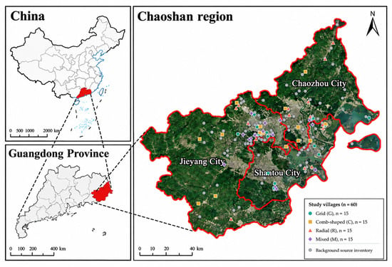
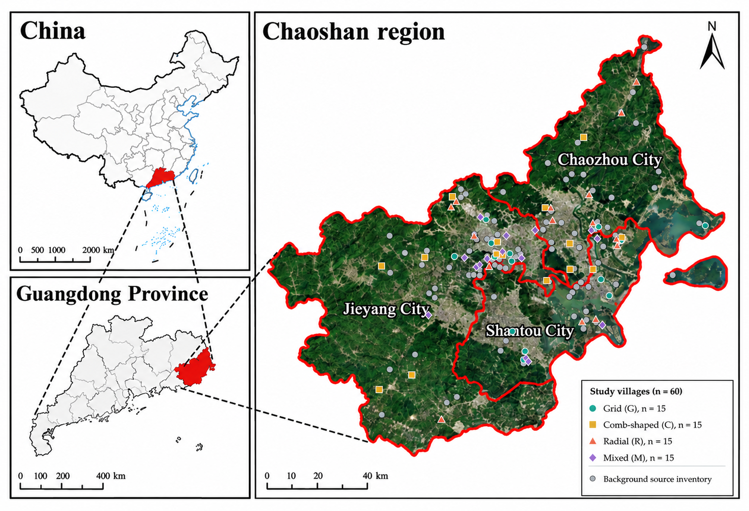
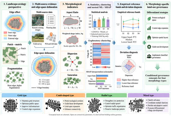
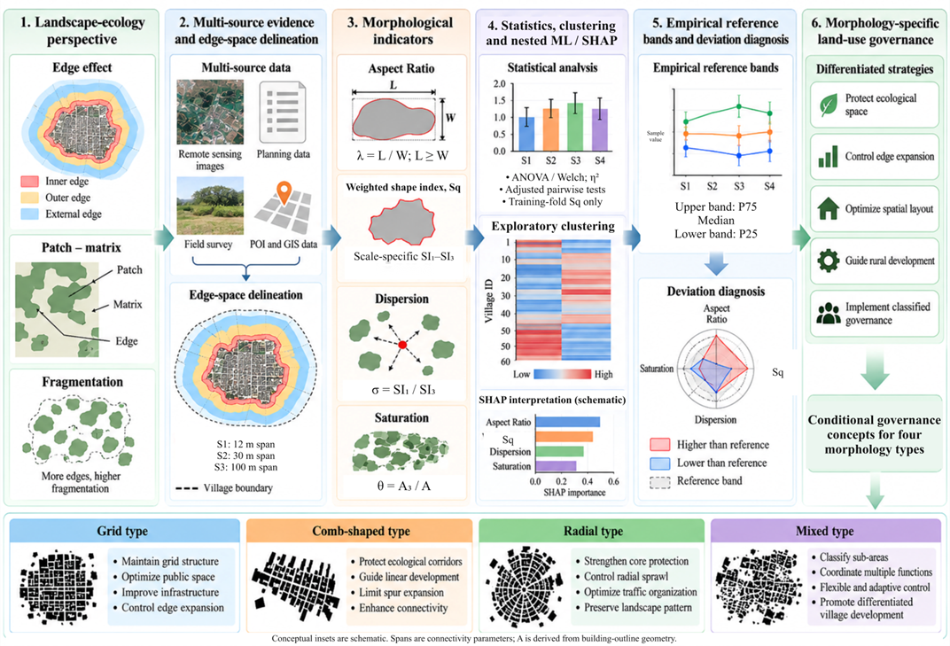
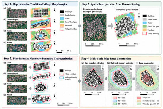
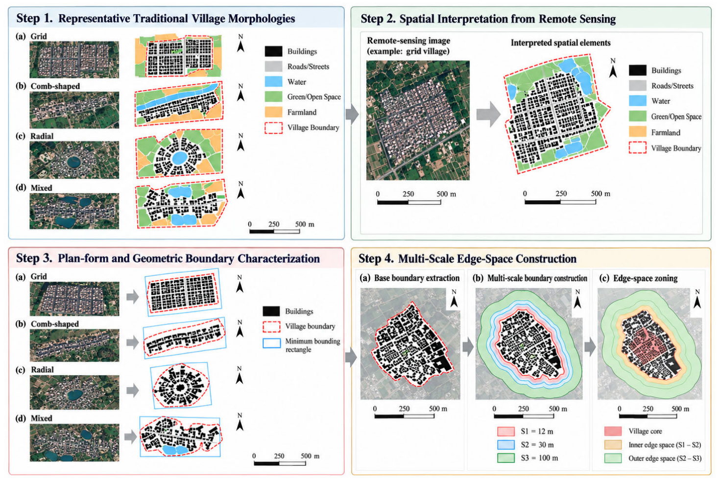
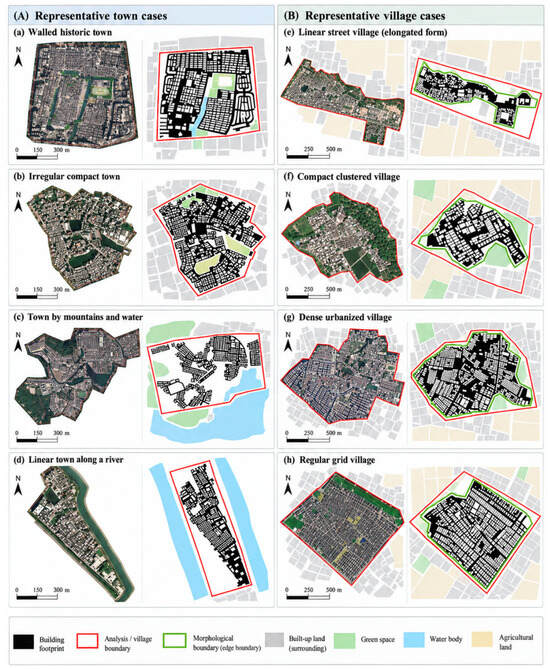
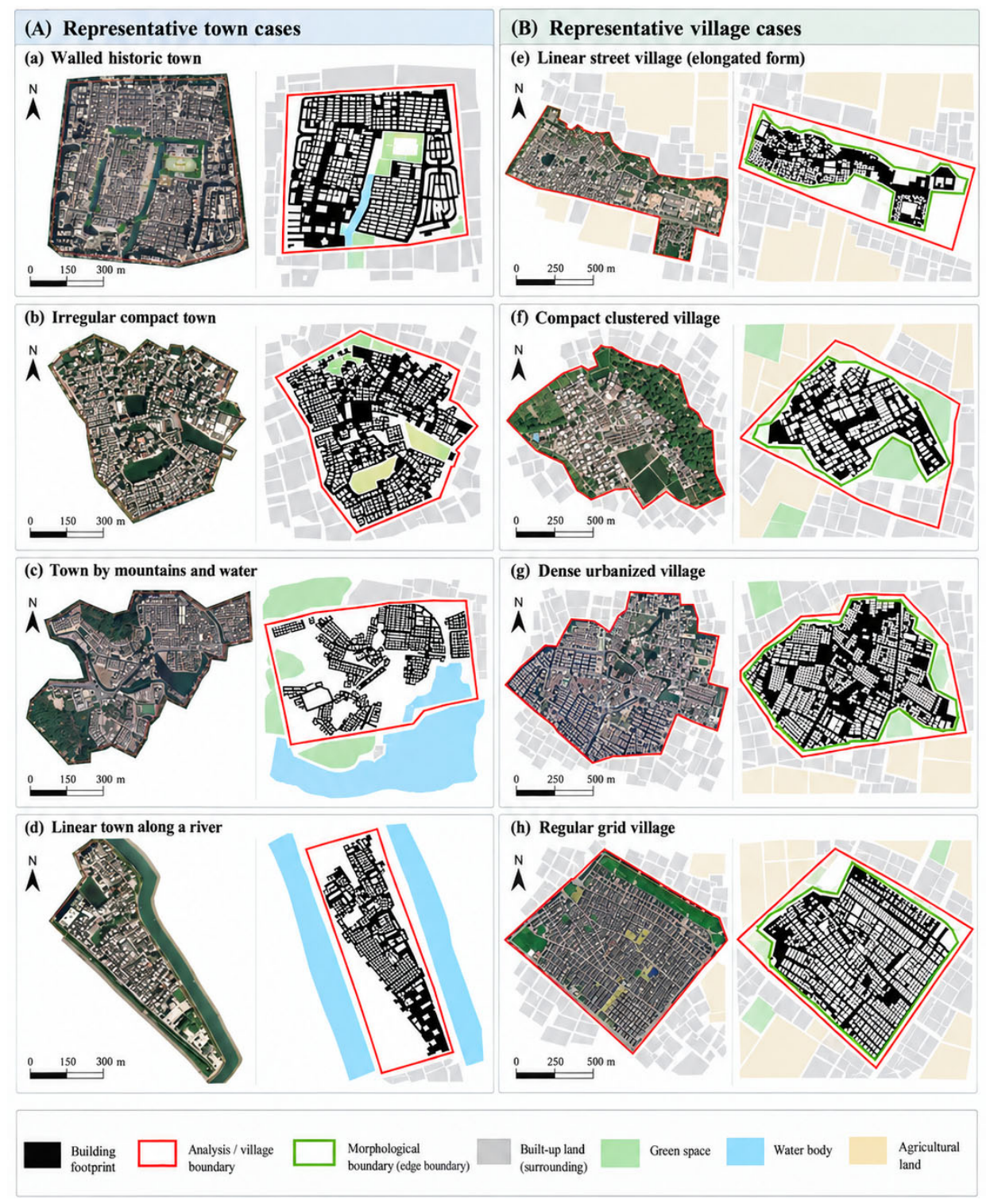
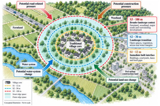
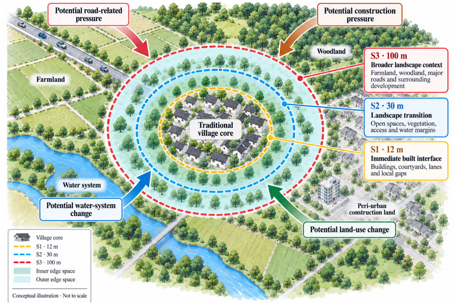
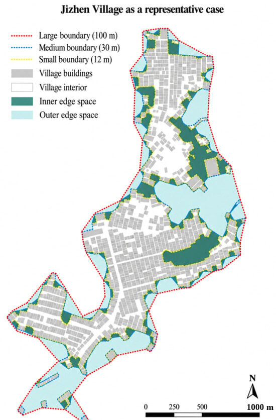
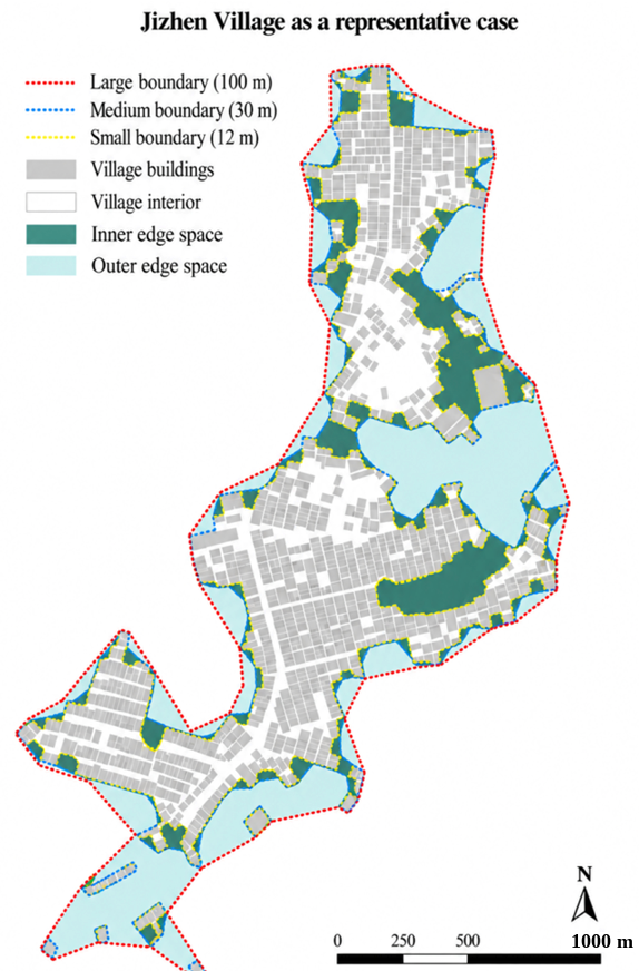
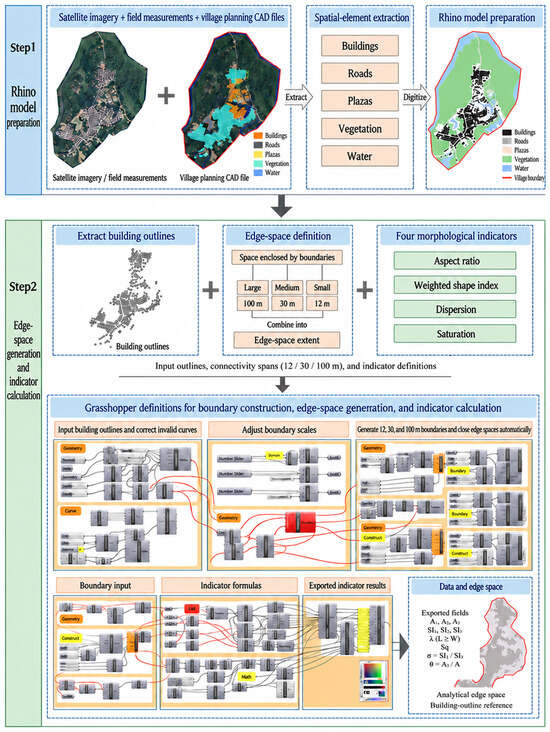
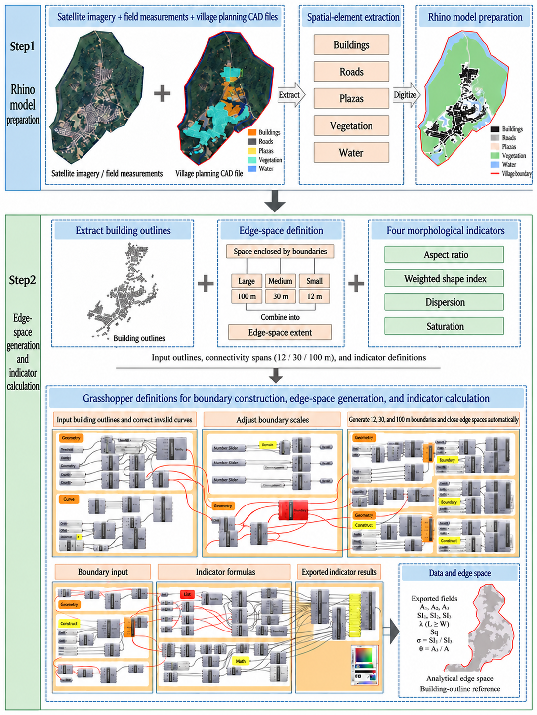
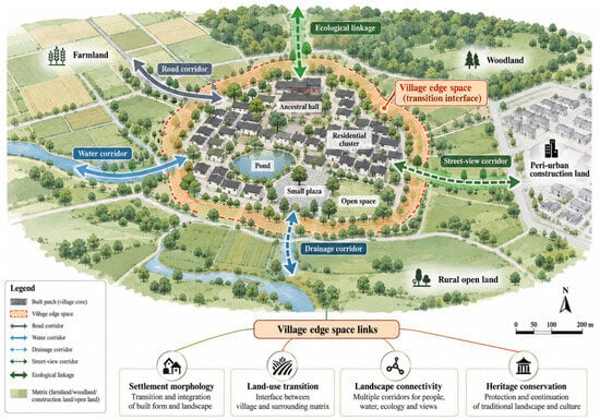
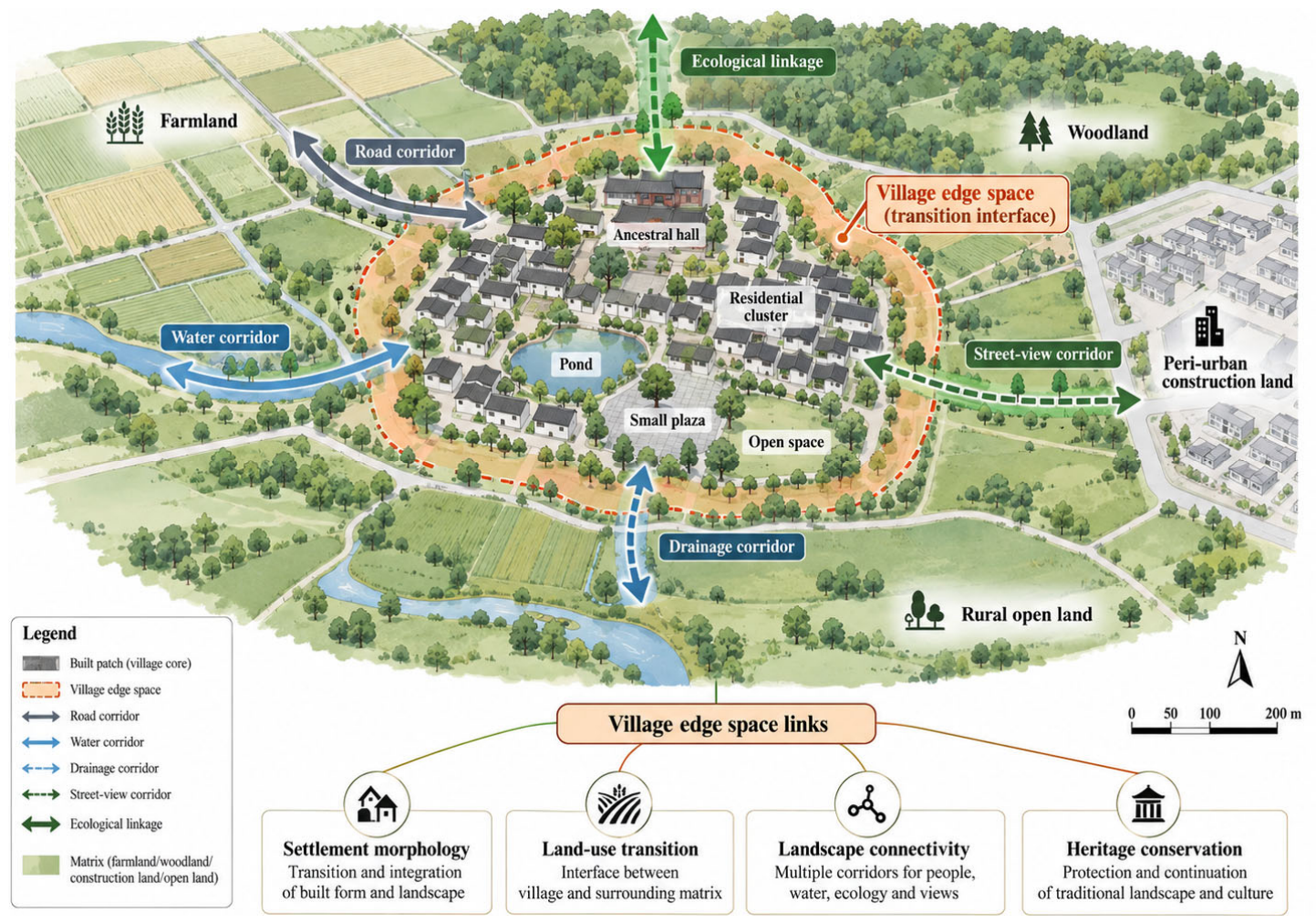
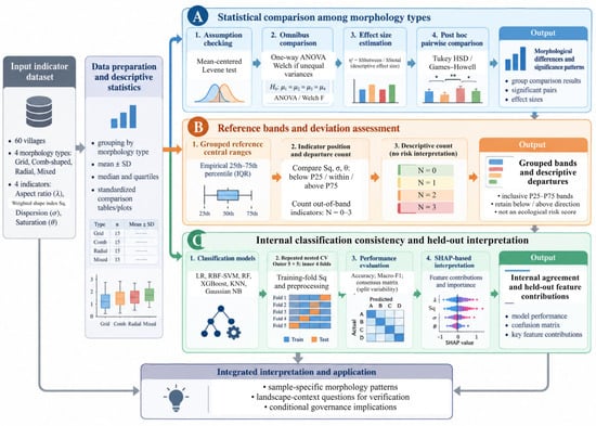
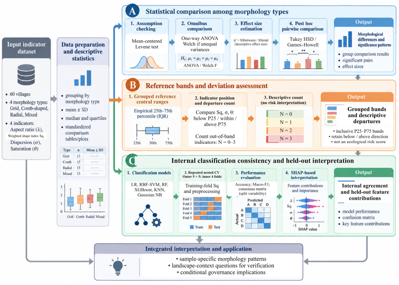
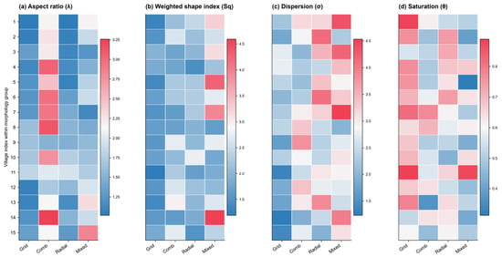
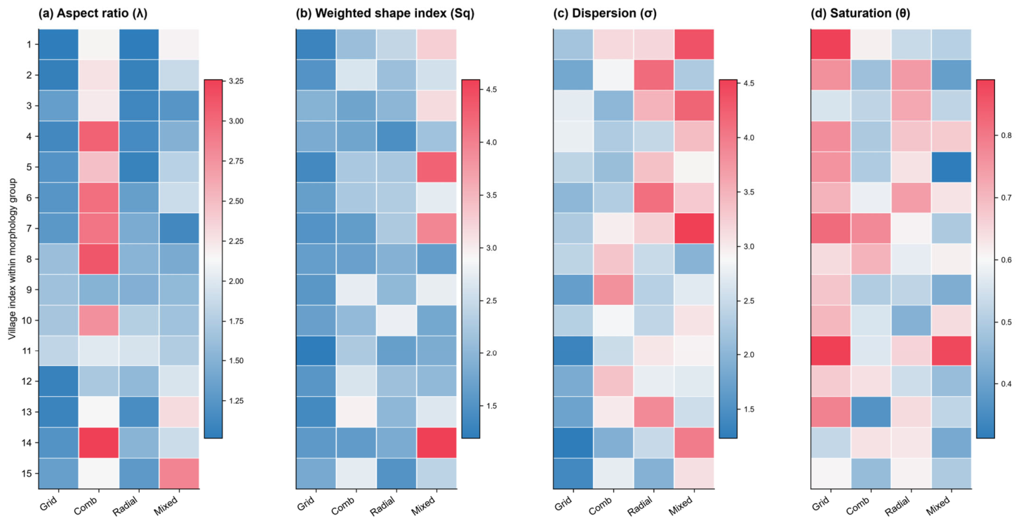
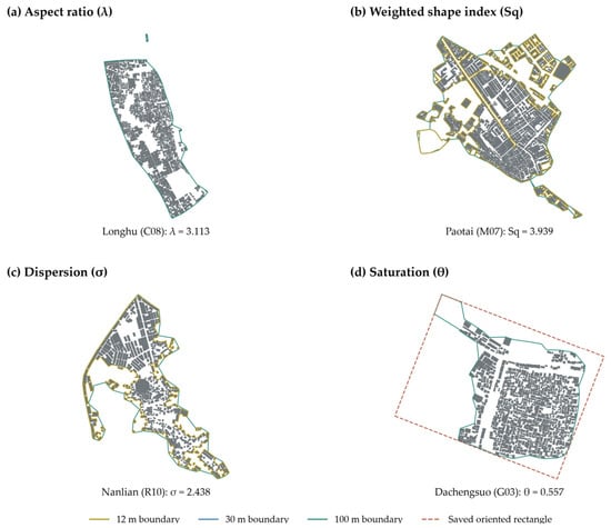
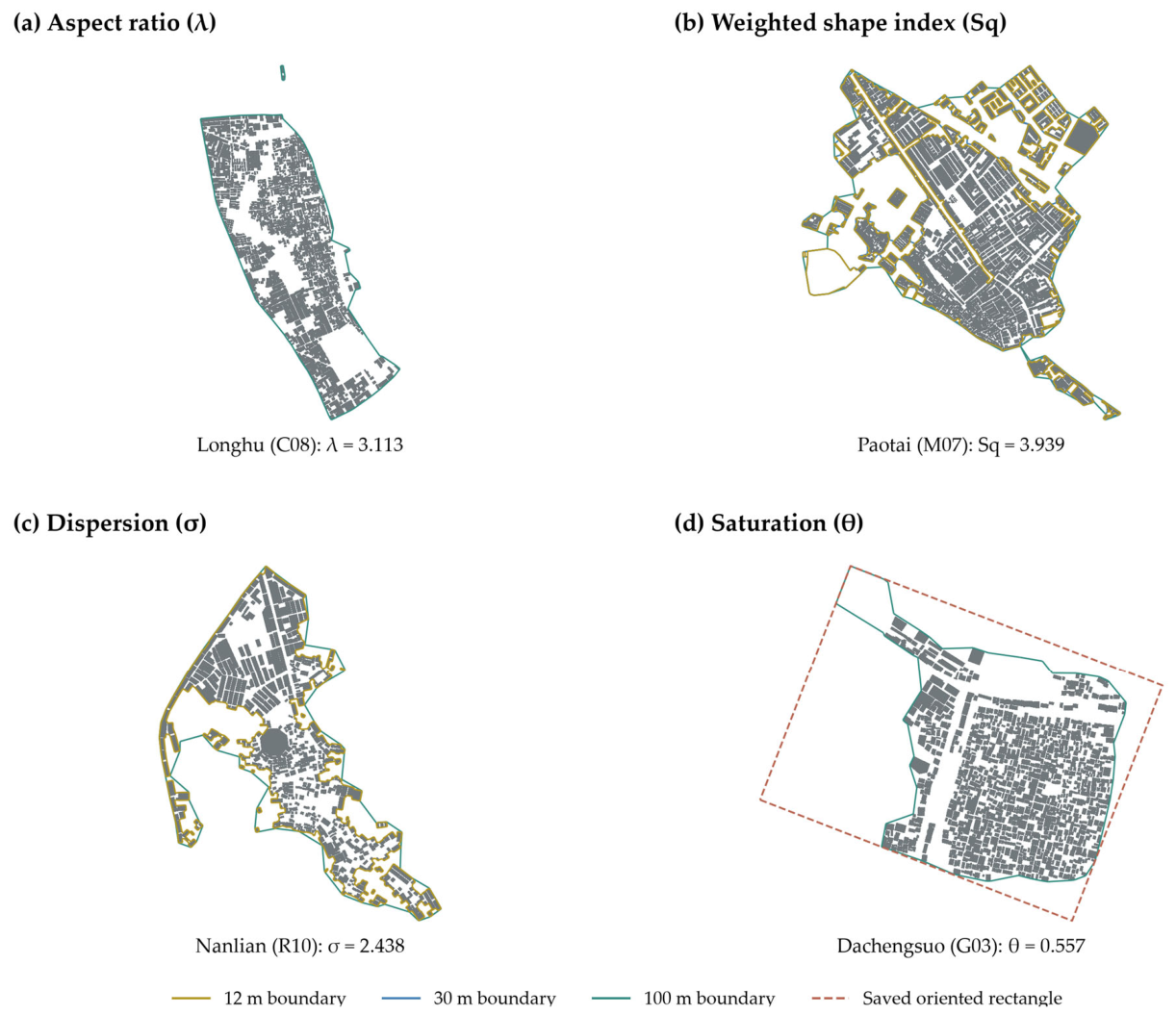
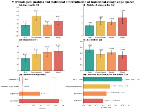
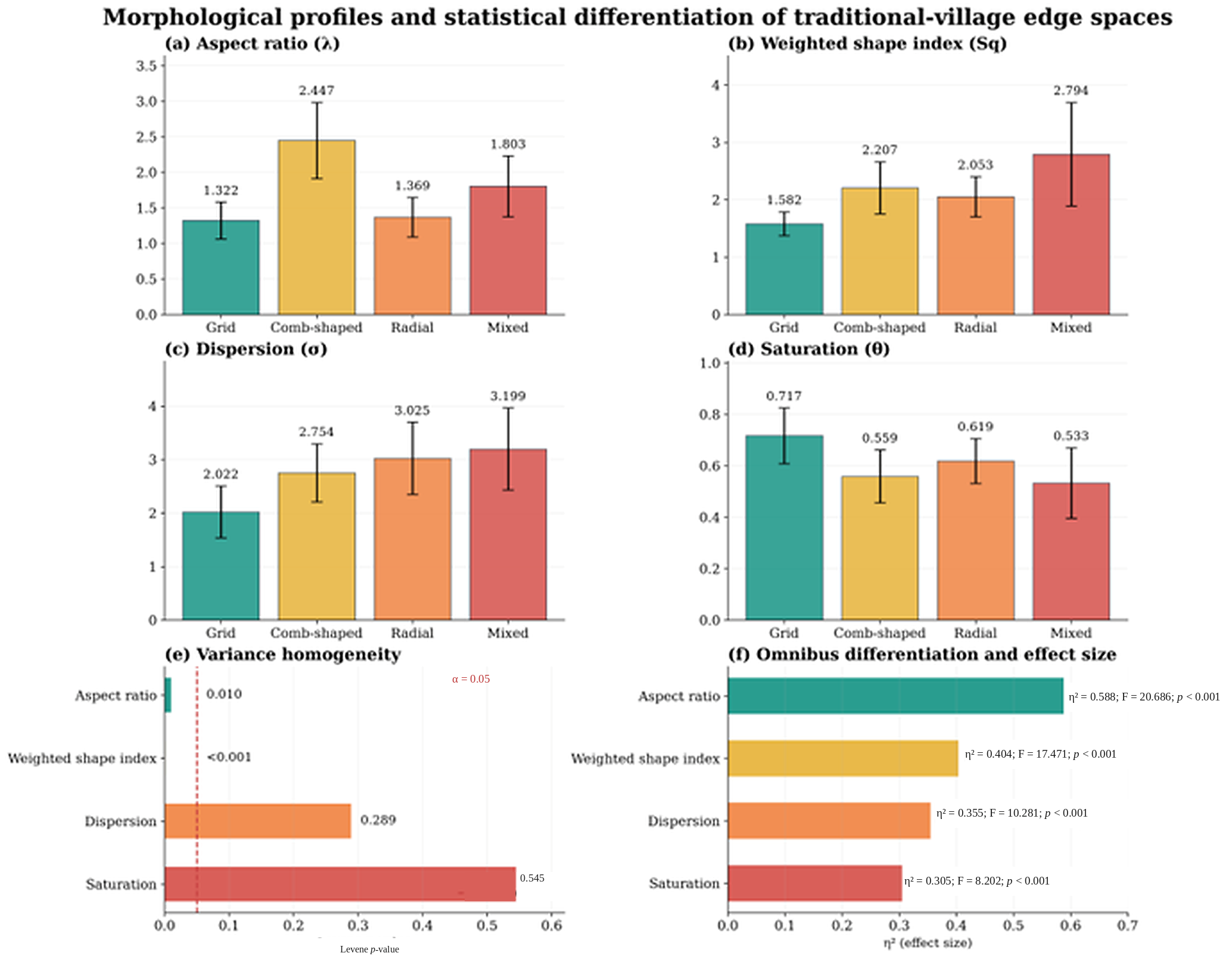
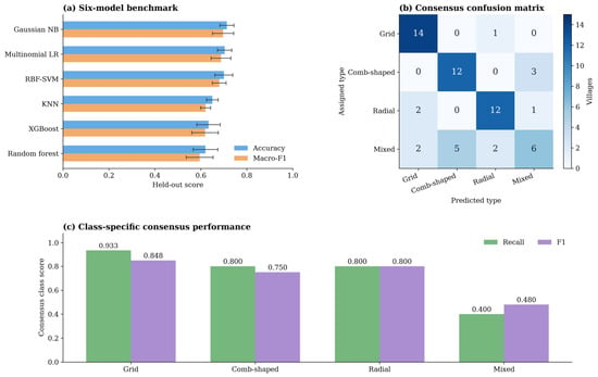
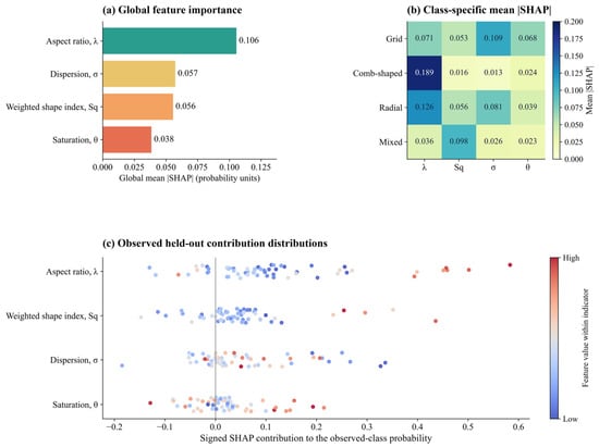
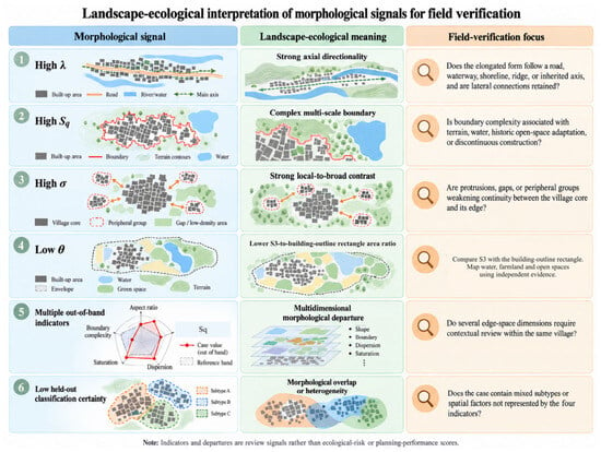
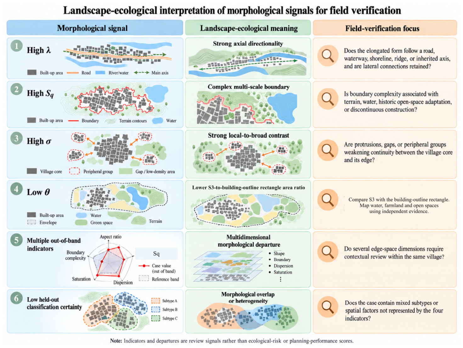
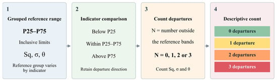
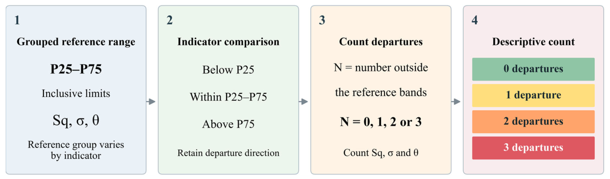
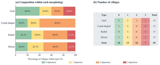
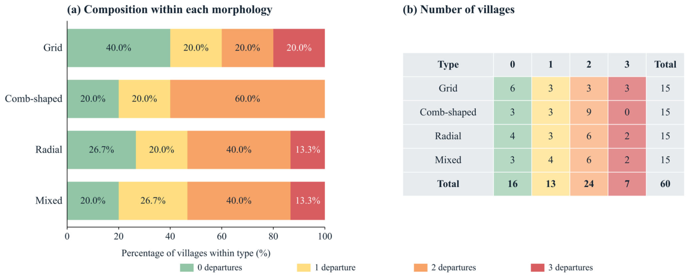
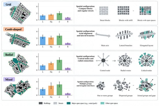
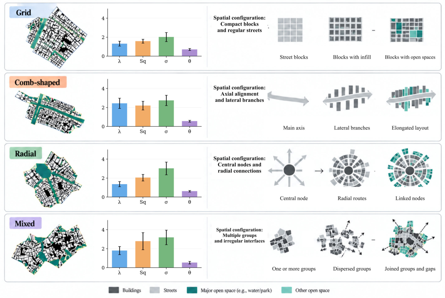
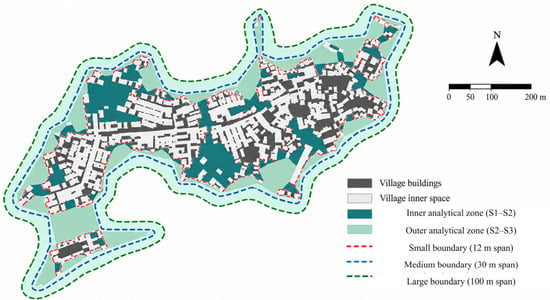
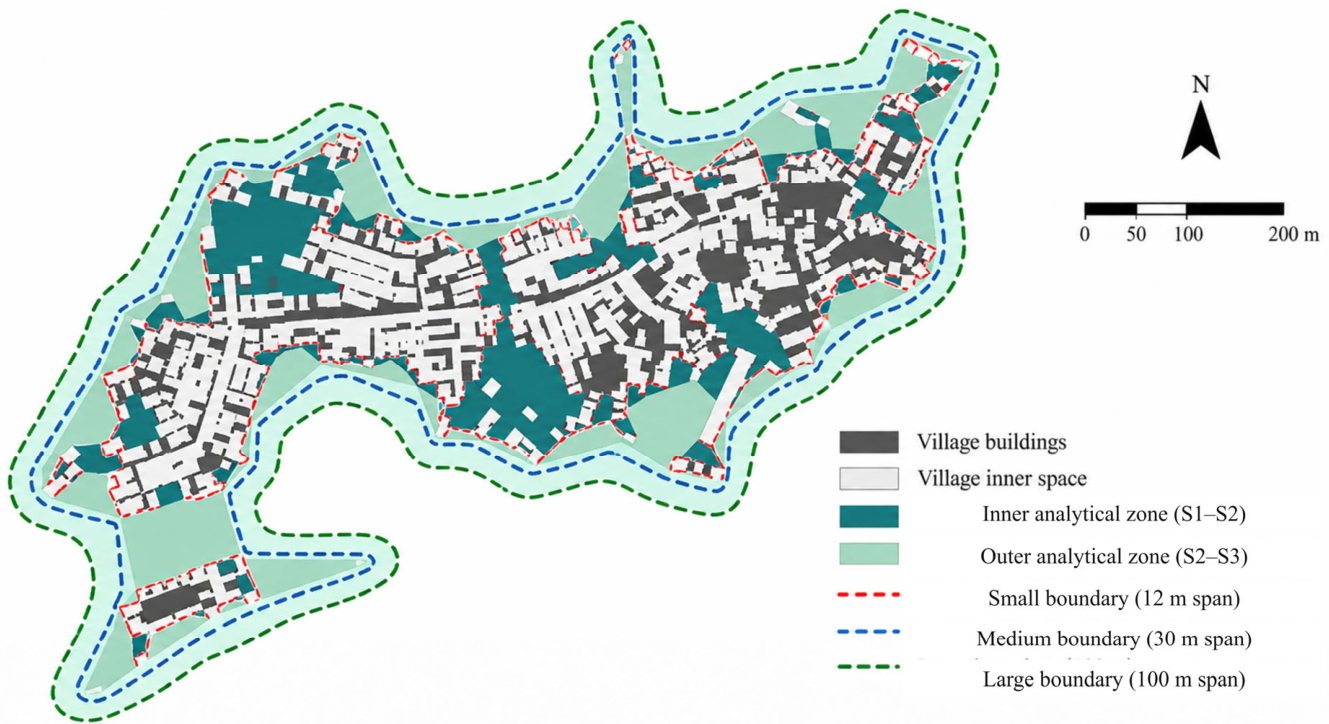
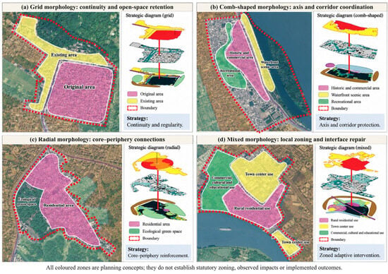
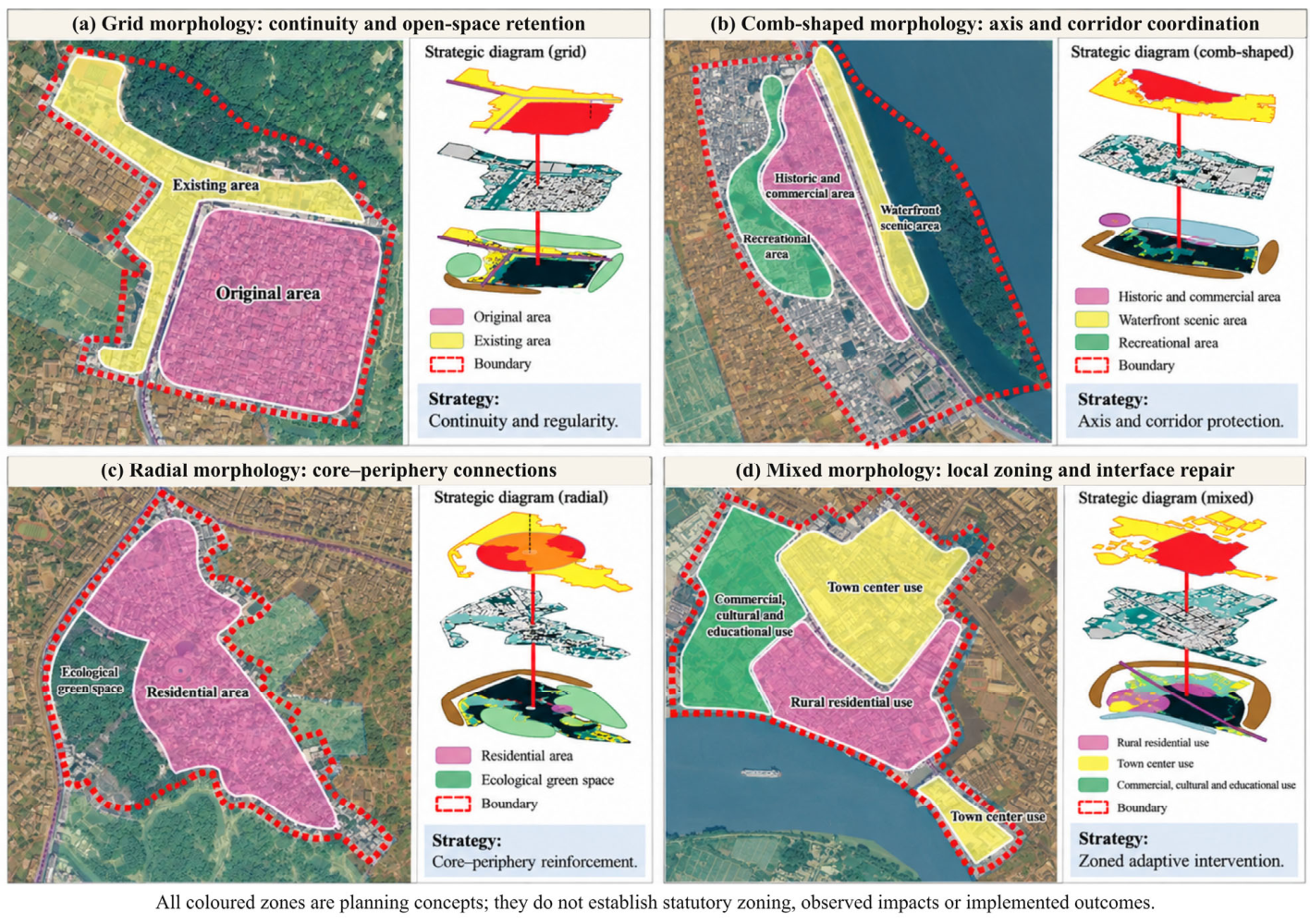
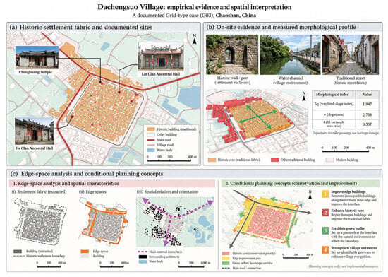
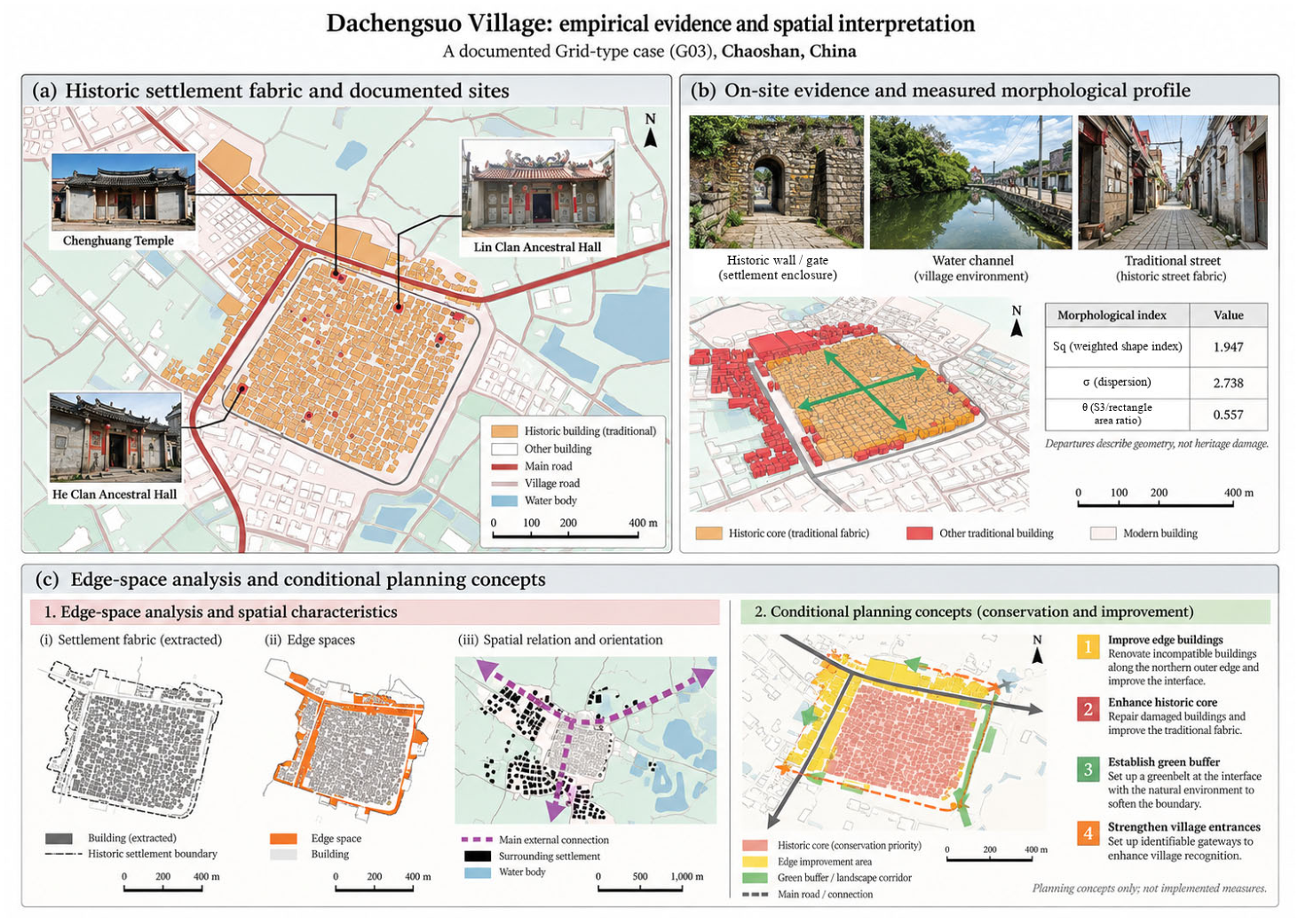
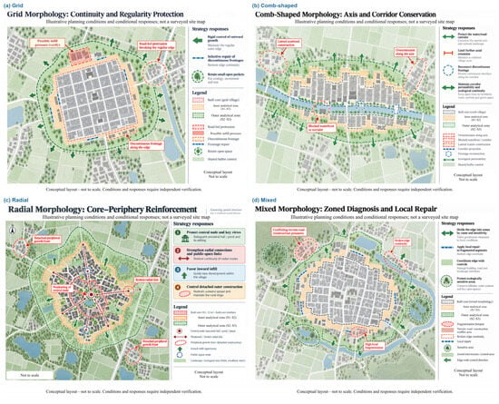
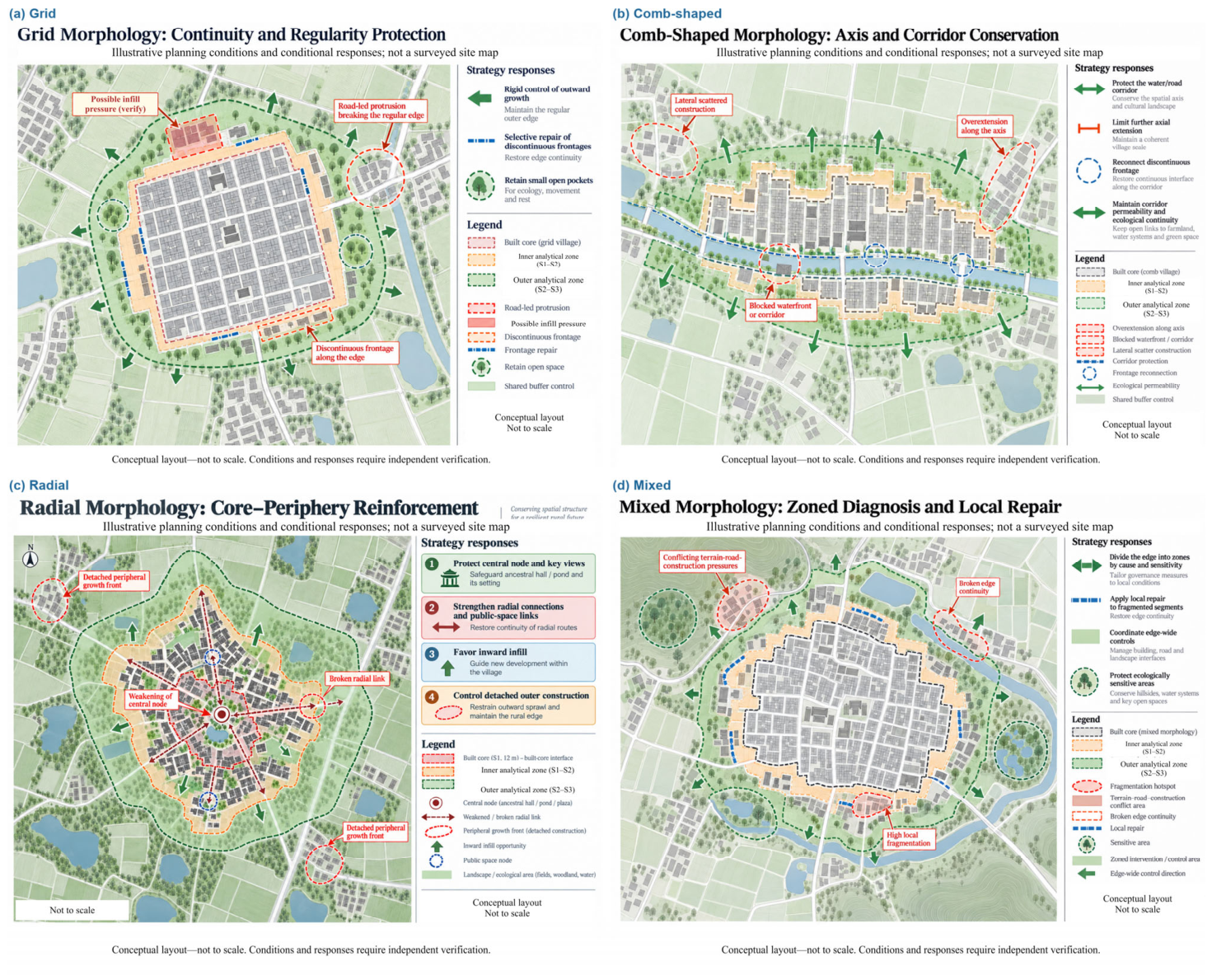

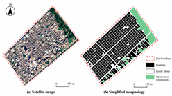
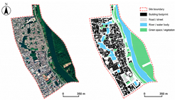
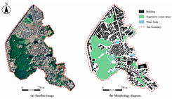
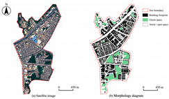
Disclaimer/Publisher’s Note: The statements, opinions and data contained in all publications are solely those of the individual author(s) and contributor(s) and not of MDPI and/or the editor(s). MDPI and/or the editor(s) disclaim responsibility for any injury to people or property resulting from any ideas, methods, instructions or products referred to in the content. |
© 2026 by the authors. Licensee MDPI, Basel, Switzerland. This article is an open access article distributed under the terms and conditions of the Creative Commons Attribution (CC BY) license.