


Abstract
Soil organic carbon (SOC) is a major terrestrial carbon pool, and its maintenance is important for climate change mitigation. Straw retention is widely used in croplands, but the association between crop residue cover (CRC) and soil organic carbon density (SOCD) may be nonlinear and may vary under peri-urban thermal conditions. We integrated multi-source spatial datasets for Mollisol croplands in Northeast China to compare recent mean SOCD in the upper 20 cm between stable rural and rural-to-urban transition zones and to examine the associations among CRC, urban heat island (UHI) intensity, and SOCD. XGBoost combined with SHapley Additive exPlanations (SHAP) was used to quantify predictor importance and characterize the nonlinear contribution of CRC to predicted SOCD. Structural equation modeling and partial least squares path modeling were further used to assess statistical associations and interaction terms among CRC, daytime and nighttime UHIs, and SOCD. Mean SOCD was slightly higher in the transition zone than in the stable zone, whereas mean CRC did not differ significantly between the two zones. The contribution of CRC to predicted SOCD showed nonlinear dependence patterns in both zones, with a similar turning region at approximately 48–50% CRC. The lower-CRC patterns differed between zones, whereas CRC was strongly positively correlated with its SHAP value across the higher-CRC interval in both zones. Daytime and nighttime UHIs were associated with contrasting CRC-SHAP patterns, and the estimated interaction effects differed between the stable and transition zones. These results reveal nonlinear and spatially heterogeneous associations between CRC and SOCD under peri-urban thermal conditions and provide a basis for further temporal and process-based investigation.
1. Introduction
Soil organic carbon (SOC) constitutes the largest terrestrial carbon reservoir, and its dynamics exert a profound influence on the global carbon cycle and climate change mitigation [1,2]. Concurrently, SOC stabilization is highly sensitive to local microclimatic conditions, which regulate the rates of microbial decomposition and organic matter transformation across diverse landscapes. Although residue retention can increase SOC stocks, its relationship with residue cover may be nonlinear and may vary with local environmental conditions [3,4]. Incubation experiments and meta-analyses suggest a possible saturation point for SOC gains derived from crop residue return [5]. Low coverage rates may even speed up the breakdown of native SOC through a priming effect [6]. Nevertheless, quantitative evidence for these thresholds in large-scale field studies remains scarce [4]. Local microclimatic perturbations, including temperature anomalies and altered moisture regimes, increasingly mediate SOC trajectories in human-dominated landscapes [7]. Among these perturbations, the urban heat island (UHI) effect represents the most pronounced manifestation of rural–urban microclimatic divergence, and has emerged as a critical yet underexplored modulator of soil carbon dynamics in peri-agricultural systems.
The UHI is conventionally viewed as a negative factor in agricultural systems, primarily because it accelerates the mineralization of soil organic carbon [8]. Ecological theories, however, indicate that temperature impacts on biological processes typically follow a “bell-shaped curve”: enzyme activities and microbial metabolism possess an optimal temperature range [9,10,11]; dropping below this range limits activity, whereas exceeding it disrupts enzyme structures and metabolic balance. Whether the UHI, as a continuous warming force, produces a similar pattern of moderate stimulation at low intensity and strong suppression at high intensity is unclear [12,13]. It is also unclear whether daytime and nighttime UHIs have opposite effects on soil carbon dynamics due to differences in radiation and evaporation [14,15]. Direct evidence and mechanistic explanations are still absent [9].
Examining the autumn UHI alongside post-harvest crop residue cover (CRC) provides a seasonal context for investigating their associations with SOCD. However, whether these associations differ between stable rural and rural-to-urban transition zones remains unclear. This question is difficult to address because high-resolution datasets simultaneously covering CRC, SOC, and UHI intensity across urban–rural gradients remain limited, while traditional linear models may not adequately capture nonlinear interactions [16].
We used the Mollisol region of Northeast China as a representative study area. As a globally significant SOC hotspot undergoing rapid urban expansion, the region provides an opportunity to examine how the associations between CRC and SOCD vary across urban–rural gradients under different thermal conditions. An XGBoost model combined with SHapley Additive exPlanations (SHAP) was used to identify important predictors of SOCD, quantify their contributions to model predictions, and characterize nonlinear response patterns. Structural equation modeling (SEM) and partial least squares structural equation modeling (PLS-SEM) were further used to examine the statistical associations among CRC, UHI intensity, and SOCD. The objectives were to (1) compare SOCD and CRC between stable rural and transition zones; (2) characterize nonlinear CRC–SHAP dependence patterns in the SOCD models; and (3) examine how these patterns and the CRC–SOCD association varied with daytime and nighttime UHI intensity.
2. Materials and Methods
2.1. Study Area
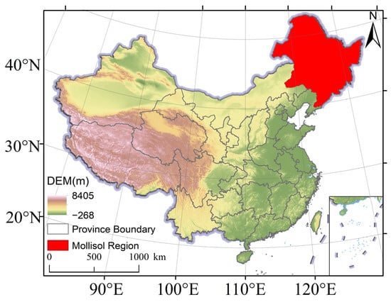
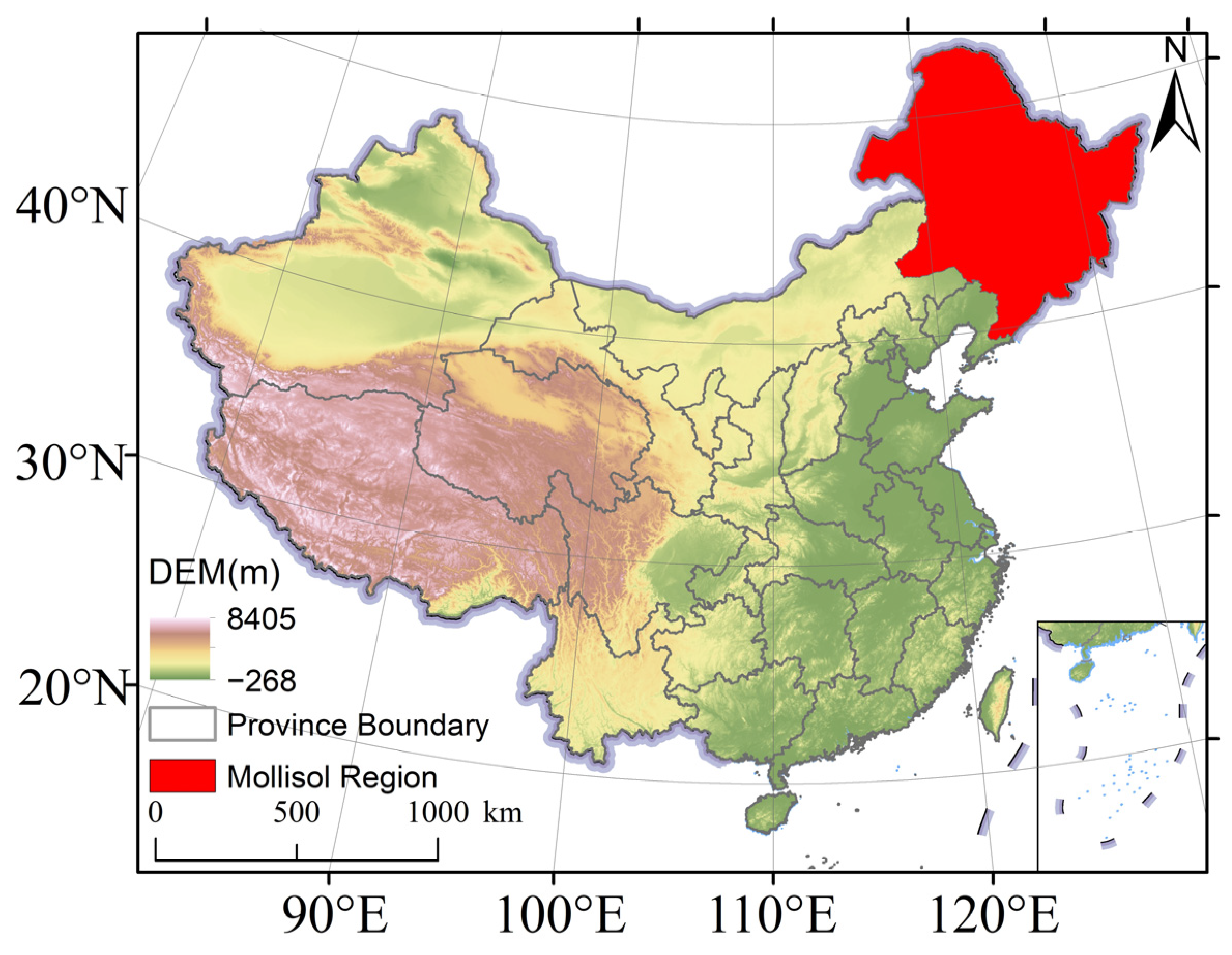
The study area encompasses the Mollisol region of Northeast China (38–53° N, 120–135° E), a globally significant SOC hotspot underlain by deep, fertile black soils (Figure 1). As one of China’s most intensively cultivated agricultural frontiers, the region simultaneously faces rapid urban expansion, which has produced extensive peri-urban transition zones where active farmland coexists with encroaching built-up land. This juxtaposition of high SOC endowment and ongoing agricultural urbanization renders the region an ideal exemplar for examining how the association between crop residue cover and SOCD varies under peri-urban thermal conditions across urban–rural gradients.
Figure 1.
Geographical location of the study area.
2.2. Data Sources and Preprocessing
2.2.1. Soil Organic Carbon Density
We used the 1 km China soil organic carbon density (SOCD) dataset [17] to characterize SOCD in the upper 20 cm of soil. In this dataset, SOCD was estimated from SOC content, bulk density, soil depth, and the coarse-fragment fraction. The dataset provides one SOCD estimate for each successive five-year period from 1985 to 2020. We averaged the estimates for 2010–2015 and 2015–2020 to characterize recent spatial patterns of 0–20 cm SOCD alongside the multi-year CRC and environmental indicators. The zonal comparison aimed to characterize spatial differences in SOCD per unit area across the urban–rural gradient. These fixed-depth differences may reflect variation in both SOC concentration and bulk density; their separate contributions were not quantified.
2.2.2. Crop Residue Cover
CRC data were obtained from the 30 m annual maize residue cover dataset for Northeast China, which covers the period from 2013 to 2021 [18]. The dataset was generated from fused Landsat and MODIS imagery using the HISTARFM method and machine learning-based estimation, and it provides CRC estimates for both the post-harvest and pre-sowing periods. We used the post-harvest product to characterize maize residue cover immediately after harvest. CRC values were converted to percentages according to the scale factor specified for the original dataset and aggregated to a spatial resolution of 1 km. To align the CRC data with the temporal coverage of the other variables, we calculated the mean post-harvest CRC for 2013–2020 and used it as the CRC indicator in subsequent analyses.
2.2.3. Urban–Rural Zonation and Nighttime Lights
Transition zones were delineated using the prolonged artificial nighttime light dataset of China (PANDA, 1984–2020), generated via a nighttime light convolutional long short-term memory network (NTLSTM) at a 1 km resolution [19]. Data from 2000 and 2020 were selected, with original DN values (scaled by 100) restored to 0–63. Referring to the established literature, a threshold of DN = 50 (i.e., 0.5) was set to identify bright urban areas. Pixels were classified into three categories: those with DN < 0.5 in 2000 and DN ≥ 0.5 in 2020 were defined as the “transition zone” (experiencing rural-to-urban transition); the remaining zones were defined as stable zones. Following spatial consistency verification with global urban boundaries across multiple threshold schemes (40–60) [20], the optimal threshold was selected. Only stable zones and transition zones were retained for analysis.
2.2.4. Urban Heat Island Intensity
UHI intensity was extracted from the 1 km resolution UHI dataset for China (2001–2023), derived from MOD11A1 land surface temperature products using urban–rural temperature differences. Autumn (September–November) UHI intensity was selected to characterize thermal conditions following maize harvest and residue retention in Northeast China. Compared with the annual mean UHI, this seasonal measure more closely matches the post-harvest CRC indicator and avoids averaging these conditions with those outside the selected period. The autumn daytime and nighttime UHI values for 2010, 2015, and 2020 were averaged to obtain UH_day_mean and UH_night_mean, respectively, expressed in °C.
2.2.5. Soil, Climate, and Topographic Data
Soil attributes, including available nitrogen (AN), clay, sand, pH, and cation exchange capacity (CEC) at 5–15 cm, were sourced from public Chinese soil datasets [21]. Climatic variables, encompassing AT and precipitation, were derived from the 1991–2020 climatological mean raster dataset [22]. Additionally, topographic relief amplitude (RA) was used to characterize terrain complexity at a 1 km resolution. All variables were uniformly resampled to 1 km and clipped to the Mollisol region.
2.3. Spatial Data Processing and Pattern Analysis
To unify the multi-source spatial framework, a 1 km × 1 km regular fishnet was constructed across the Mollisol region. With SOCD rasters as the spatial baseline, all raster data were extracted to the fishnet via pixel-center sampling to generate a structured attribute table. Automatic projection transformation and bilinear resampling ensured spatial alignment. Ultimately, each grid contained a comprehensive variable set: SOCD, CRC_mean, zonation identifier (UrbanTransition: 1 = transition zone, 0 = stable zone), soil attributes, climate, topography, and UHI intensity. The full dataset comprised approximately 1.6 million valid grids (1.59 million stable rural, 0.0027 million transition zone grids).
We employed a space-for-time substitution framework to interpret spatial gradients in UHI intensity and CRC, drawing on its application in land-use carbon research [23]. Within this framework, spatial gradients in UHI intensity and CRC are assumed to serve as proxies for potential temporal trajectories of SOCD change. This interpretation assumes that cropland locations with contrasting UHI intensities and CRC levels represent different conditions along a potential temporal continuum after accounting for the environmental covariates included in the models.
CRC and SOCD distributions were compared between the stable and transition zones. Mann–Whitney U tests were used to assess differences at the α = 0.05 significance level.
2.4. XGBoost-SHAP for Key Driver and Threshold Identification
To identify critical drivers of SOCD and capture their potential nonlinear effects, XGBoost regression models were constructed [24,25]. XGBoost is a scalable Gradient Boosting Decision Tree algorithm that sequentially adds new trees to correct the residuals of prior predictions, effectively capturing complex nonlinear relationships and high-order interactions among predictors. The algorithm minimizes a regularized loss function composed of a differentiable convex loss term measuring the discrepancy between observed and predicted values and a regularization term that penalizes model complexity to prevent overfitting. Its objective function is formally expressed as
where l denotes the loss function (squared error for regression), and are the observed and predicted values for the i-th sample, respectively, and represents the k-th decision tree. Optimization proceeds via second-order Taylor expansion of the loss function, enabling efficient computation of the regularized gradient and accelerating model convergence. A learning rate (shrinkage) further controls the step size of each tree update. Crucially, the ensemble tree-based structure of XGBoost is intrinsically robust to multicollinearity, allowing the retention of all selected environmental features without inflating model variance or compromising predictive stability [26].
In the present study, SOCD_2010_2020_mean was designated as the dependent variable, and 11 independent variables spanning CRC, soil properties (AN, Clay, Sand, pH, CEC), climate (AT, Precipitation), topography (RA), and UHI intensity (UH_night_mean, UH_day_mean) served as predictors. Recognizing the distinct ecological processes operating across the urban–rural gradient, separate models were independently developed for the stable zone and the transition zone. The dataset was randomly partitioned into training (70%) and test (30%) subsets. Hyperparameter optimization was conducted via Bayesian optimization (Tree-structured Parzen Estimator) to identify the optimal combination of key parameters, including the number of estimators, maximum tree depth, learning rate, subsample ratio, and column sampling fraction, using root mean square error (RMSE) on a validation fold as the minimization target. Final model performance on the held-out test set was evaluated through the coefficient of determination (R2) and RMSE.
Despite their superior predictive accuracy, machine learning models are often criticized for their limited interpretability [27]. To address this, SHapley Additive exPlanations (SHAP) [28] was applied to decompose the contribution of each predictor to individual SOCD predictions. SHAP assigns each feature an importance value for each sample, derived from cooperative game theory, where the marginal contribution of a feature is averaged over all possible feature orderings. The mean absolute SHAP value across all test samples was employed to quantify the overall importance of each factor, providing a consistent and additive measure of feature contribution to model predictions. SHAP summary plots were generated to visualize both the direction and magnitude of each feature’s influence, while SHAP dependence plots were utilized to reveal the nonlinear functional form of key predictors—particularly CRC_mean—on SOCD. To further examine the hypothesized moderating role of UHI in the CRC–SOCD association, SHAP dependence scatter plots of CRC were colored by UHI intensity (UH_night_mean or UH_day_mean), and stratified dependence curves were constructed for low and high UHI quartiles. This analysis was used to characterize nonlinear and context-dependent relationships in the SOCD predictions. All machine learning and SHAP analyses were implemented in Python (version 3.9.25) using the xgboost (version 2.1.4) and shap (version 0.49.1) packages.
2.5. SEM and PLS-SEM Analysis
SEM was used to examine the associations among CRC, UHI intensity, and SOCD while accounting for the selected environmental covariates. Interaction terms were included to assess whether the CRC-SOCD association varied with daytime and nighttime UHI intensity. The structural specification of the models is fundamentally anchored in the biogeochemical dynamics of agroecosystems undergoing urbanization. Diurnal UHI, nocturnal UHI, and CRC were established as the primary explanatory variables, while specific edaphic, climatic, and topographic control variables were integrated to account for baseline ecosystem heterogeneity. By incorporating interaction terms (CRC × UH_night, CRC × UH_day), the model estimates the main associations and interaction terms linking CRC and UHI intensity with SOCD [29,30].
A covariance-based SEM (CB-SEM) was constructed exclusively for the stable zone to evaluate the specified path model. Given the smaller sample size in the transition zone (N = 432), a variance-based PLS-SEM was executed for exploratory path analysis. The PLS-SEM specifically focused on the core paths associated with SOCD, namely the direct effects of mean diurnal UHI (UH_day_mean) and mean CRC (CRC_mean), coupled with their specific interaction (CRC × UH_day).
The fundamental objective of CB-SEM is to minimize the discrepancy between the observed sample covariance matrix and the covariance matrix implied by the specified model. Model parameters were derived via maximum likelihood estimation using the Python package semopy. To facilitate the direct comparison of relative effect magnitudes across variables possessing disparate units, all estimated path coefficients were strictly standardized. Furthermore, the R2 was computed to quantify the proportion of spatial variance in SOCD elucidated by the associations. Model fit was rigorously evaluated, relying upon the Comparative Fit Index (CFI), Tucker–Lewis Index (TLI), Root Mean Square Error of Approximation (RMSEA), and Chi-square statistic.
Ultimately, these structural models were used to quantify the associations of CRC and UHI intensity with SOCD and to complement the nonlinear patterns identified by XGBoost-SHAP.
3. Results
3.1. Spatial Patterns of CRC and SOCD Across Urban–Rural Gradients
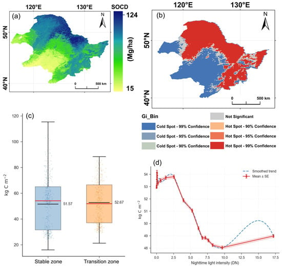
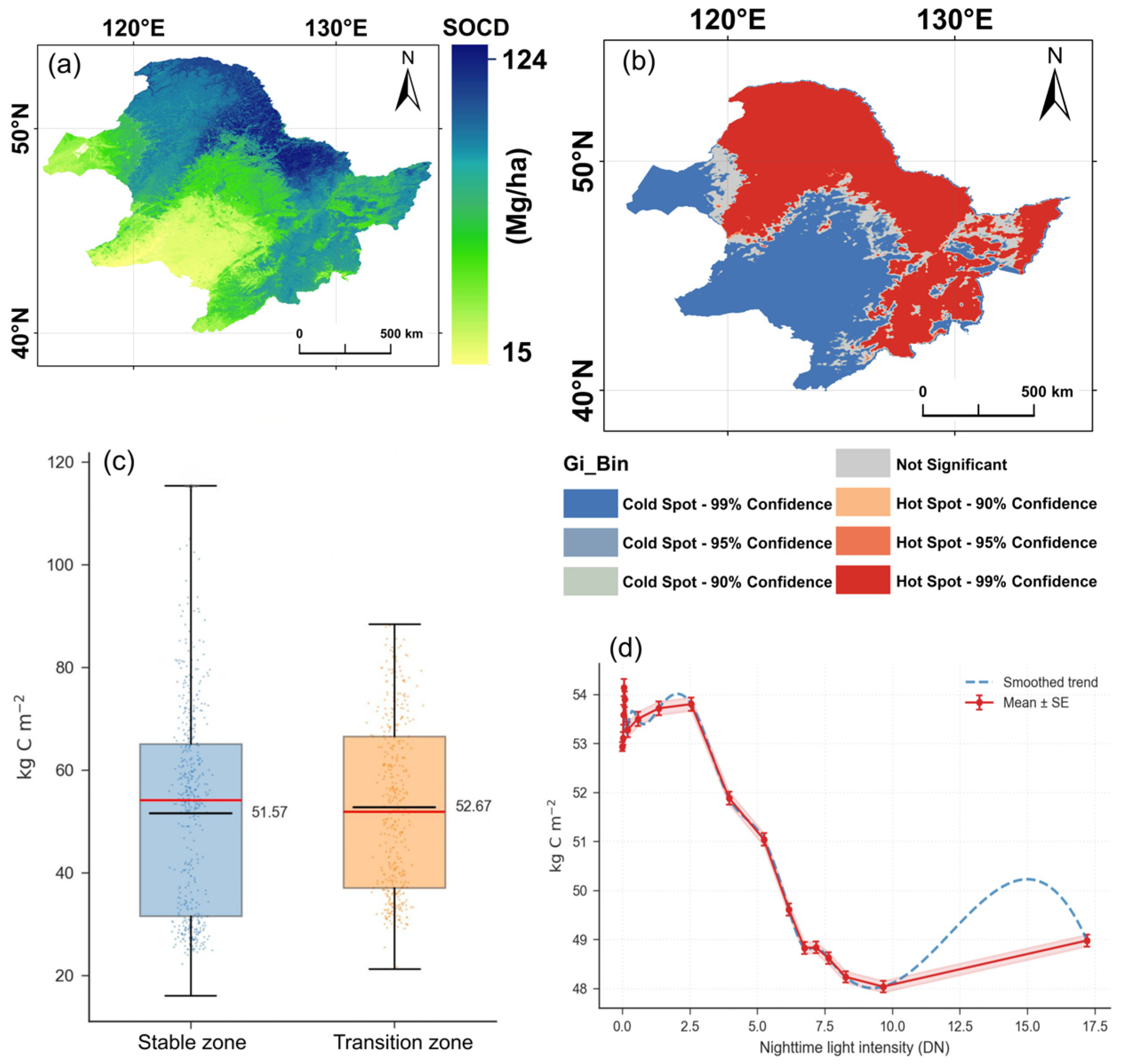
Based on the nighttime-light zonation, we compared SOCD between the stable zone (n = 362,775) and the rural-to-urban transition zone (n = 432). Mean SOCD was 51.57 Mg C ha−1 (SD = 19.16) in the stable zone and 52.67 Mg C ha−1 (SD = 16.59) in the transition zone, corresponding to a mean difference of 1.10 Mg C ha−1 (Table 1). The lower standard deviation in the transition zone indicates lower variability in SOCD. The Mann–Whitney U test showed that the SOCD distributions differed significantly between the two zones (U = 72,687,921, p = 0.009).
Table 1.
Descriptive statistics and difference testing of SOCD across urban–rural zonation.
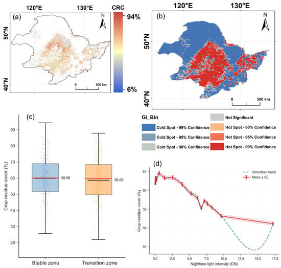
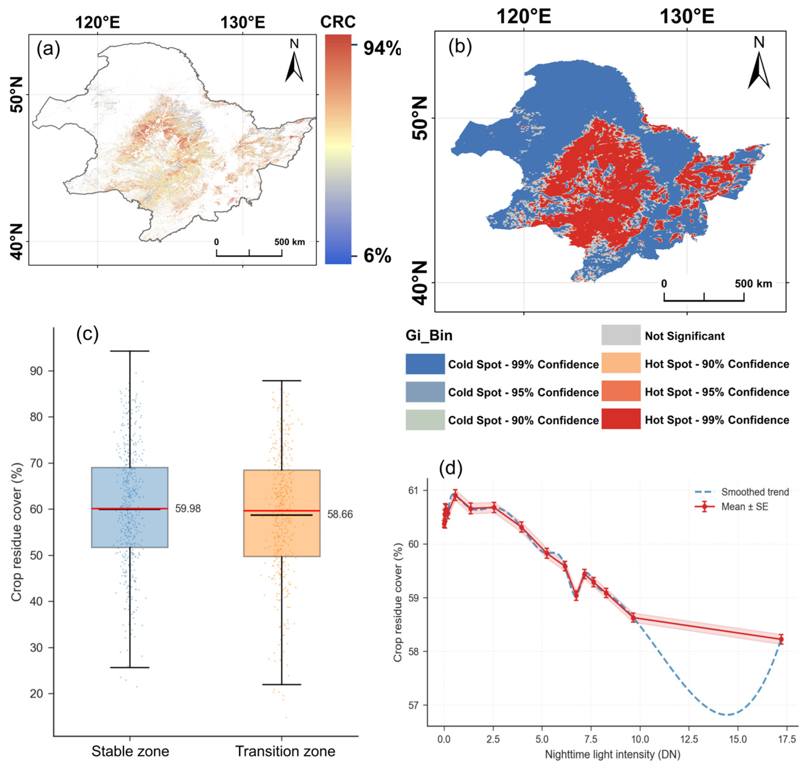
Though SOCD distributions differed significantly between the two zones (Figure 2), CRC showed no significant zonal difference (Figure 3). Mean CRC was 59.98% (SD = 13.18%) in the stable zone and 58.66% (SD = 14.01%) in the transition zone (Table 2). The Mann–Whitney U test indicated that the CRC distributions did not differ significantly between the two zones (U = 81,999,605, p = 0.095). Given the similar CRC levels but different SOCD distributions, subsequent analyses examined whether the modeled relationship between CRC and SOCD varied between the stable rural and transition zones.
Figure 2.
Spatial pattern characteristics of SOCD across the urban–rural gradient. (a) Spatial distribution map of SOCD; (b) Getis-Ord hotspot–coldspot clustering map for SOCD; (c) box-and-whisker plot comparing SOCD values between stable zone and transition zone; (d) variation trend in SOCD along the nighttime-light intensity gradient (DN value). Error bars represent mean ± standard error (SE); blue dashed line denotes smoothed trend.
Figure 3.
Spatial patterns of CRC across the urban–rural gradient. (a) Spatial distribution of crop residue cover (CRC, %); (b) Getis-Ord hotspot–coldspot clustering map for CRC; (c) box-and-whisker plot comparing CRC values between stable zone and transition zone; (d) variation trend in CRC along the nighttime-light intensity gradient (DN value). Error bars represent mean ± standard error (SE); blue dashed line denotes smoothed trend.
Table 2.
Statistics and difference testing of CRC across urban–rural zonation.
3.2. Contributions of CRC to SOCD and Nonlinear Effects
3.2.1. Relative Contributions
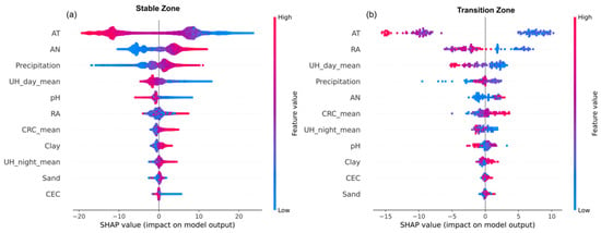
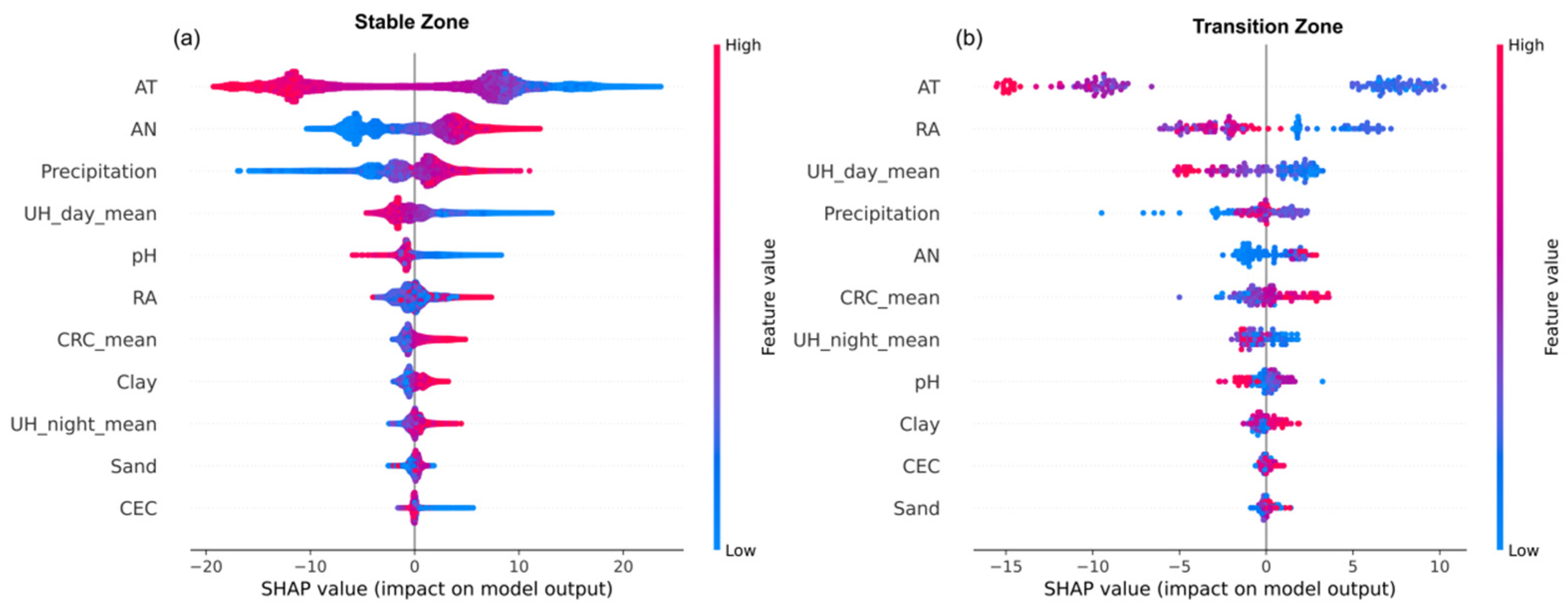
The XGBoost models achieved strong predictive fidelity in both zones (Figure 4), with an R2 of 0.914 and RMSE of 5.62 kg C ha−2 in the stable zone and an R2 of 0.879 with RMSE of 5.30 kg C ha−2 in the transition zone. Mean absolute SHAP values were extracted to rank feature importance (Table 3). AT dominated in both regions (|SHAP| > 9), indicating the importance of the regional thermal regime for SOCD prediction. Beyond this overarching climatic control, distinct zonal signatures emerged. In the stable zone, AN ranked second (|SHAP| = 4.168), reflecting the tight coupling between soil nutrient status and higher predicted SOCD in conventional farmland. The transition zone displayed a fundamentally different hierarchy. RA rose to second (|SHAP| = 3.479), suggesting that topographic context may be particularly relevant to SOCD variation in the transition zone. Concurrently, daytime UHI intensity (UH_day_mean) climbed to third (|SHAP| = 2.220), substantially higher than its ranking in the stable zone, indicating a greater predictive role for daytime UHI in the transition zone. Notably, the mean |SHAP| of CRC was higher in the transition zone (1.229) than in the stable zone (0.910), indicating a larger mean absolute contribution of CRC to the transition-zone SOCD predictions.
Figure 4.
SHAP summary plots illustrating feature effects on SOCD prediction for two zones. (a) SHAP summary plot for the stable zone; (b) SHAP summary plot for the transition zone. The x-axis represents SHAP values denoting feature contributions to SOCD prediction. The color gradient encodes feature values (red = high feature value; blue = low feature value). Variables are vertically ordered according to the magnitude of the mean absolute SHAP values (feature importance).
Table 3.
Mean absolute SHAP values, indicating predictor importance for soil organic carbon density prediction in the stable rural and transition zones.
3.2.2. Nonlinear CRC-SHAP Dependence Patterns
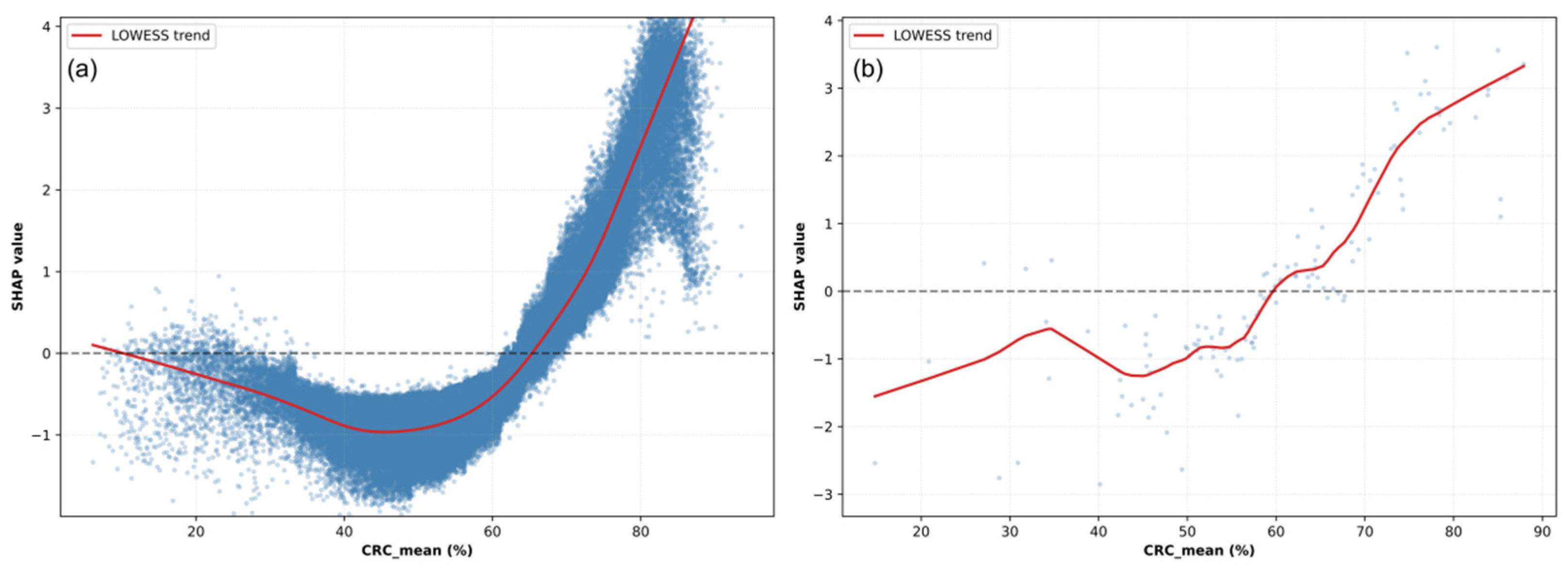
In the stable zone, CRC ranged from 6.1% to 93.6%, and individual CRC SHAP values ranged from −2.12 to 4.86. CRC was positively correlated with its SHAP value overall (r = 0.785), indicating that higher CRC generally contributed to higher SOCD predictions relative to the model baseline. However, the dependence pattern was nonlinear. In the lower-CRC interval, the CRC-SHAP correlation was negative (r = −0.483), and the fitted dependence curve reached a minimum SHAP value of −1.36 at approximately 48.6% CRC. In the higher-CRC interval, CRC was strongly positively correlated with its SHAP value (r = 0.971), and the fitted curve reached a maximum SHAP value of 3.59 at approximately 81.6% CRC. The mean CRC SHAP value across the stable zone was −0.009 (Figure 5).
Figure 5.
SHAP dependence plot for CRC. (a) Stable zone; (b) transition zone. The x-axis shows mean crop residue cover (CRC_mean, %), and the y-axis shows the contribution of CRC_mean to predicted SOCD relative to the respective model baseline. Blue scatter points correspond to individual observations; the solid red line indicates the LOWESS smoothed trend curve; the horizontal dashed line at SHAP = 0 represents zero predictive contribution.
In the transition zone, CRC ranged from 14.8% to 87.9%, and individual CRC SHAP values ranged from −5.00 to 3.61. The overall correlation between CRC and its SHAP value was positive (r = 0.876). The lower-CRC interval showed a weak positive correlation (r = 0.310), whereas a strong positive correlation was observed in the higher-CRC interval (r = 0.927). The fitted dependence curve reached a minimum SHAP value of −2.42 at approximately 48.4% CRC and a maximum SHAP value of 3.05 at approximately 77.2% CRC. The mean CRC SHAP value across the transition zone was 0.143.
3.2.3. Regional Comparison
Both zones showed nonlinear CRC-SHAP dependence patterns (Table 4), with the fitted curves reaching their minimum values at similar CRC levels of approximately 48.6% in the stable zone and 48.4% in the transition zone. In the lower-CRC interval, CRC was negatively correlated with its SHAP value in the stable zone (r = −0.483) but weakly positively correlated with its SHAP value in the transition zone (r = 0.310). In the higher-CRC interval, strong positive CRC-SHAP correlations were observed in both zones (r = 0.971 and 0.927, respectively). The overall CRC-SHAP correlation was higher in the transition zone (r = 0.876) than in the stable zone (r = 0.785). Individual CRC SHAP values ranged from −5.00 to 3.61 in the transition zone and from −2.12 to 4.86 in the stable zone. These SHAP values represent contributions to the respective model predictions relative to each model’s baseline.
Table 4.
Characteristics of the nonlinear CRC–SHAP dependence patterns in the stable rural and transition zones.
3.3. CRC-SHAP Patterns Across UHI Intensity Quartiles
Stratifying the dataset by UHI intensity quartiles enabled an examination of CRC SHAP values across thermal conditions, thereby examining how the modeled CRC-SOCD relationship varies across distinct thermal regimes.
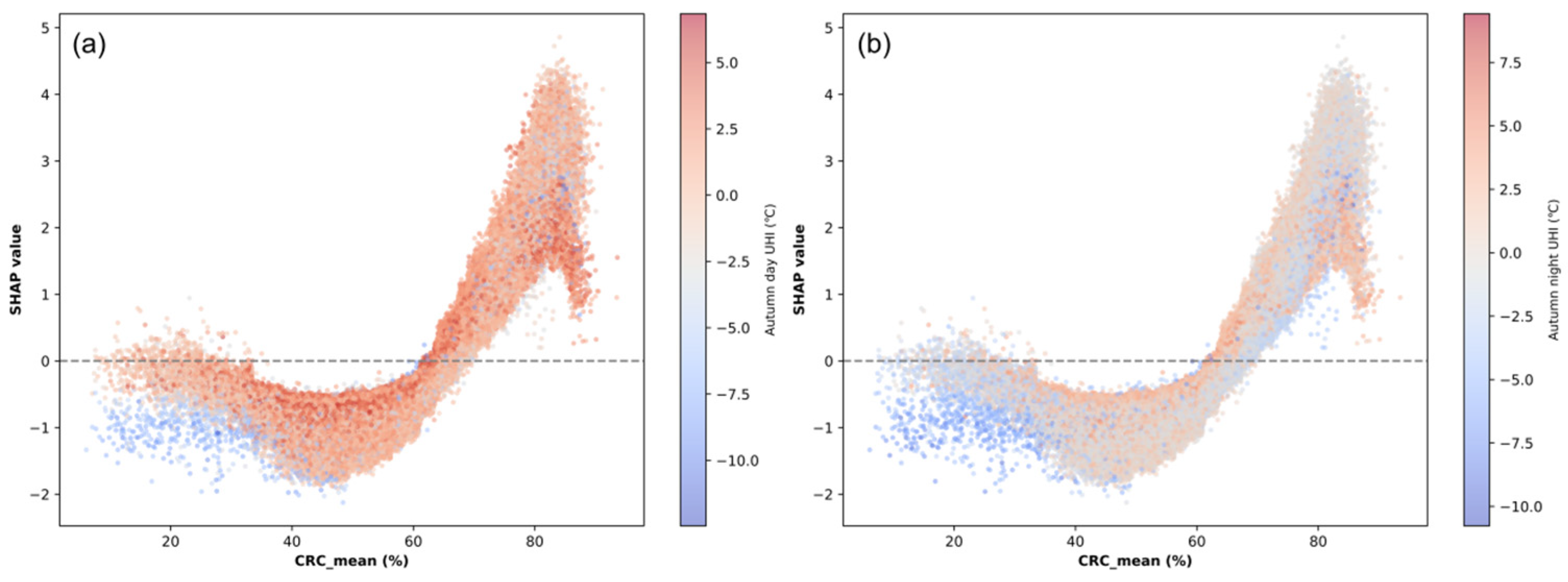
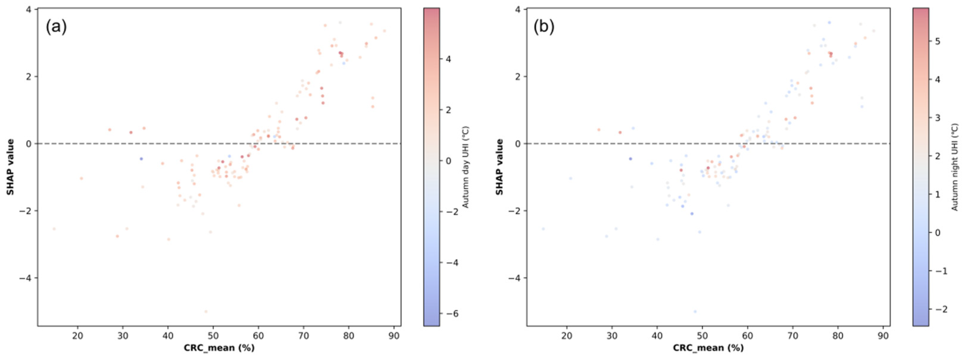
Across the nocturnal UHI quartiles in the stable zone, the CRC-SHAP correlation strengthened progressively from 0.750 (Q1) to 0.833 (Q4) (Table 5; Figure 6). This pattern indicates a stronger CRC–SHAP correlation at higher nighttime UHI intensity. However, the mean SHAP shifted from a positive 0.125 in the lowest UHI quartile to a plateau of approximately −0.05 in Q2–Q4. Elevated nighttime UHI was associated with a stronger CRC-SHAP correlation but a lower mean CRC SHAP value. Diurnal UHI exhibited a contrasting trajectory. The CRC-SHAP correlation rose initially, peaking at 0.840 in Q3, before retreating to 0.813 in Q4. Meanwhile, the mean CRC SHAP value decreased overall from 0.133 (Q1) to −0.210 (Q4). The strongest daytime CRC–SHAP correlation occurred in Q3, whereas the mean CRC SHAP contribution was lowest in Q4.
Table 5.
CRC-SHAP statistics across daytime and nighttime UHI quartiles in the stable zone.
Figure 6.
SHAP dependence plots of CRC_mean colored by autumn urban heat island intensity for the stable zone. (a) CRC-SHAP dependence colored by autumn daytime UHI intensity (°C); (b) CRC-SHAP dependence colored by autumn nighttime UHI intensity (°C). X-axis: Mean crop residue cover (CRC_mean, %); Y-axis: SHAP values representing marginal contribution of CRC_mean to SOCD prediction. Color gradient encodes UHI intensity (red for high UHI, blue for low UHI). The horizontal dashed line at SHAP = 0 denotes zero contribution to the SOCD prediction relative to the model baseline.
Within the transition zone, CRC-SHAP patterns varied across UHI quartiles and differed between daytime and nighttime conditions (Figure 7; Table 6). Under nighttime UHI, the CRC-SHAP correlation increased from 0.694 in Q1 to a maximum of 0.909 in Q3 and then decreased to 0.782 in Q4. The mean CRC SHAP value increased from −0.241 in Q1 to a maximum of 0.459 in Q3 and remained positive at 0.442 in Q4. Under daytime UHI, the CRC-SHAP correlation increased from 0.782 in Q1 to a maximum of 0.949 in Q2, and subsequently decreased to 0.709 in Q4. In contrast, the mean CRC SHAP value varied from −0.391 in Q1 to its highest value of 0.515 in Q4. Thus, the UHI quartile associated with the strongest CRC-SHAP correlation differed between daytime and nighttime conditions, and the daytime correlation maximum did not coincide with the highest mean CRC SHAP value.
Figure 7.
SHAP dependence plots of CRC_mean colored by autumn urban heat island intensity for the transition zone. (a) CRC-SHAP dependence colored by autumn daytime UHI intensity (°C); (b) CRC-SHAP dependence colored by autumn nighttime UHI intensity (°C). X-axis: Mean crop residue cover (CRC_mean, %); Y-axis: SHAP values representing marginal contribution of CRC_mean to SOCD prediction. Color gradient encodes UHI intensity (red for high UHI, blue for low UHI). The horizontal dashed line at SHAP = 0 denotes zero contribution to the SOCD prediction relative to the model baseline.
Table 6.
CRC-SHAP statistics across daytime and nighttime UHI quartiles in the transition zone.
3.4. Path Analysis of CRC, UHI Intensity, and SOCD
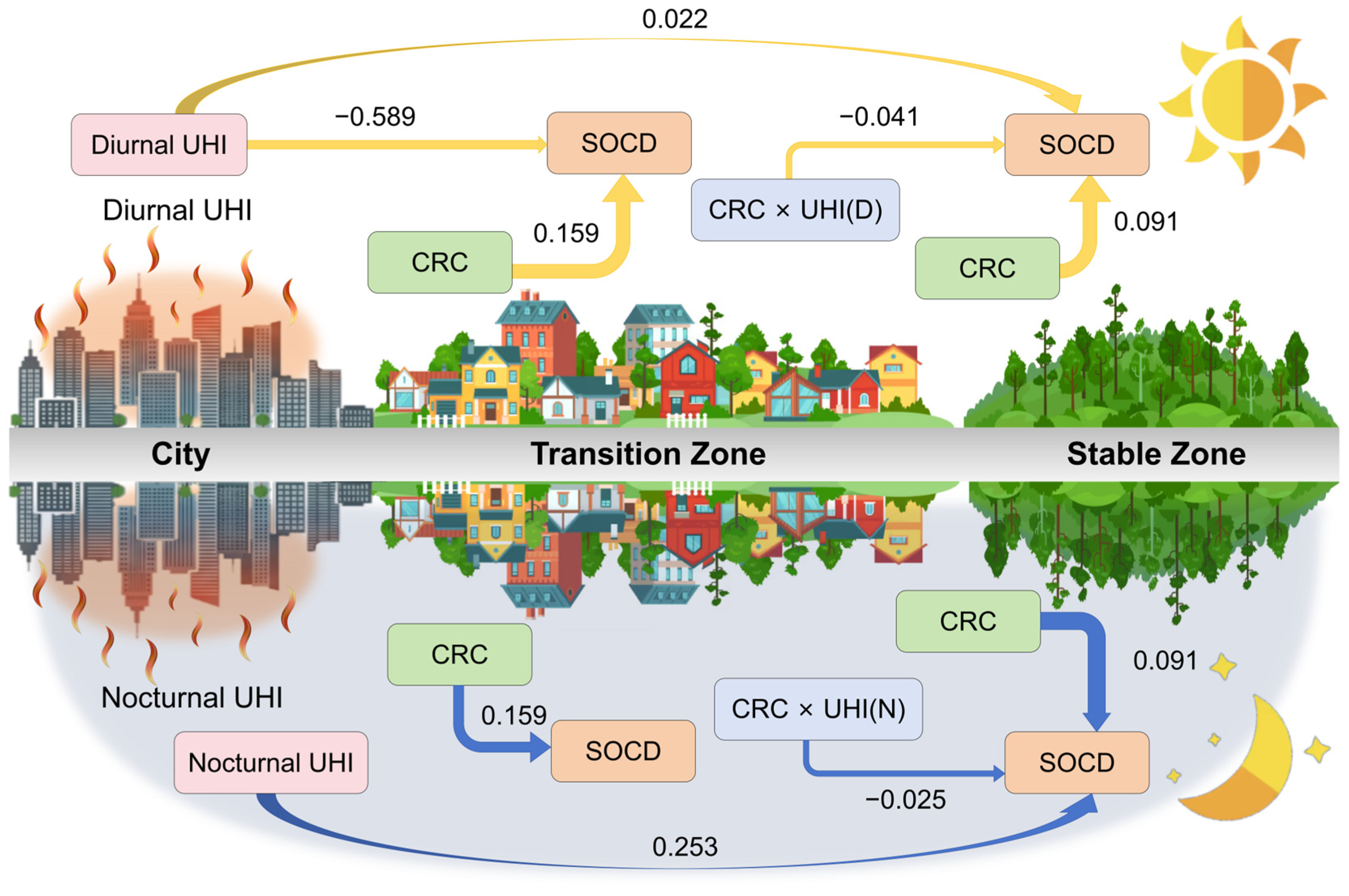
The XGBoost-SHAP analysis showed that CRC-SHAP patterns varied across UHI intensity levels, although these patterns remained predictive in nature. To further examine the statistical associations among CRC, UHI intensity, and SOCD, a covariance-based SEM was fitted for the stable zone, whereas PLS-SEM was used for exploratory path analysis in the transition zone (Figure 8).
Figure 8.
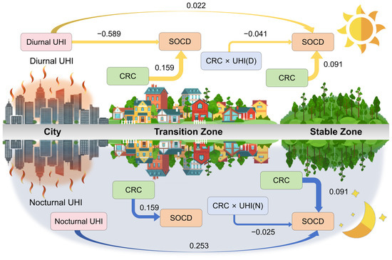
Estimated paths among CRC, UHI intensity, and SOCD in the stable rural and transition zones. The upper panel presents paths involving daytime UHI, and the lower panel presents paths involving nighttime UHI. Path estimates for the stable zone were obtained using covariance-based SEM, whereas those for the transition zone were obtained using PLS-SEM. Standardized path coefficients are shown beside the arrows. Yellow and blue arrows indicate paths involving daytime and nighttime UHI, respectively. Boxes represent the variables included in the models.
Following the XGBoost-SHAP analysis, a covariance-based SEM was fitted for the stable zone (n = 108,822), with climatic, edaphic, and topographic variables included as covariates. The model explained 81.2% of the variance in SOCD (R2 = 0.812), with CFI = 1.000, TLI = 1.000, and RMSEA < 0.001. The standardized path coefficients from CRC, nighttime UHI, and daytime UHI to SOCD were positive (β = 0.091, 0.253, and 0.022, respectively; all p < 0.001; Table 7). The coefficient for the CRC × daytime UHI interaction was negative (β = −0.041, p < 0.001), as was the coefficient for the CRC × nighttime UHI interaction (β = −0.025, p < 0.001). Within the fitted model, these negative interaction coefficients indicate that the positive association between CRC and SOCD became weaker as UHI intensity increased. The daytime interaction coefficient was larger in absolute magnitude than the nighttime interaction coefficient.
Table 7.
Key path coefficients of the SEM in the stable zone.
Given the smaller sample size in the transition zone (n = 432), PLS-SEM was used for exploratory path analysis. The model explained 41.6% of the variance in SOCD (R2 = 0.416), and all reported path coefficients were statistically significant. The standardized path coefficient from daytime UHI to SOCD was negative (β = −0.589), whereas the corresponding coefficient was small and positive in the stable zone (β = 0.022). The CRC × daytime UHI interaction coefficient was also negative in the transition zone (β = −0.159), consistent in direction with the negative interaction coefficient estimated for the stable zone (β = −0.041). Although the absolute value of this interaction coefficient was larger in the transition zone, the difference should be interpreted descriptively because the two estimates were obtained using different modeling frameworks and substantially different sample sizes.
4. Discussion
4.1. Nonlinear Effects of CRC on SOCD
The results reveal a pronounced nonlinear association between CRC and its contribution to predicted SOCD in both the stable rural and transition zones. The fitted CRC-SHAP dependence curves showed similar turning regions at approximately 48–50% CRC, beyond which the contribution of CRC to predicted SOCD increased markedly. This pattern suggests that the relationship between residue cover and SOCD may depend on the level of surface cover rather than following a simple linear trend. Although the turning region should not be interpreted as a universally applicable management threshold, its consistent position in the two zones points to a potentially meaningful shift in the modeled CRC-SOCD relationship.
The observed pattern is broadly consistent with previous studies showing that SOC responses to residue retention depend on the amount of residue retained and the surrounding management conditions [31,32,33]. Under relatively low residue cover, limited organic carbon inputs may be insufficient to support a detectable positive contribution to SOCD, while residue-induced priming and the associated mineralization of native SOC may also contribute to the negative CRC SHAP values observed in the stable zone [31]. At higher residue-cover levels, greater residue-derived carbon inputs and improved soil microenvironmental conditions may favor SOC retention, potentially explaining the increasingly positive CRC contributions to predicted SOCD [32,33]. These processes provide plausible biogeochemical explanations for the nonlinear pattern, although their relative importance requires further field-based evaluation.
The difference between the two zones in the lower-CRC interval further suggests that the CRC-SOCD relationship is modified by the surrounding environmental context. The stable zone showed a negative CRC-SHAP correlation at lower CRC levels, whereas the transition zone showed a weak positive correlation. This contrast may reflect differences in thermal conditions, historical land management, organic matter inputs, or soil physical properties across the urban–rural gradient. Peri-urban conditions may therefore partly modify the response associated with low residue cover, although the specific contribution of each process remains uncertain. Overall, the similar turning regions in the two zones indicate a shared nonlinear response pattern, while the contrasting lower-CRC relationships highlight its context dependence.
4.2. Contrasting Daytime and Nighttime UHI Associations with the CRC–SOCD Relationship
The CRC-SHAP patterns varied with UHI intensity and differed between daytime and nighttime conditions. In the stable zone, the highest daytime UHI level was associated with a lower mean CRC SHAP value. In the transition zone, the nighttime CRC-SHAP correlation and mean SHAP value were both highest in Q3, whereas the daytime correlation was highest in Q2 and the mean SHAP value was highest in Q4. These different peak positions suggest that the UHI influence on the modeled CRC-SOCD relationship is nonlinear and cannot be represented by a single uniform thermal response.
These findings highlight the importance of distinguishing daytime and nighttime thermal conditions when examining the CRC-SOCD relationship. The differences between zones also suggest that associations identified in stable rural croplands may not fully describe those in peri-urban transition croplands [9,10,12,13].
4.3. Characteristics of the Transition Zone
The transition zone showed several characteristics that differed from those of the stable zone, including slightly higher mean SOCD, comparable mean CRC, a different predictor-importance ranking, and distinct CRC-SHAP dependence patterns. The comparable CRC levels may partly reflect the widespread use of mechanized maize harvesting and continued straw-retention practices across the study area. Continued agricultural support may also help sustain these practices in transition croplands despite urbanization pressures. Meanwhile, the observed SOCD difference may be associated with legacy soil fertility, management history, organic matter inputs, soil physical properties, and local thermal conditions. Peri-urban croplands are exposed to the combined influences of land-use transition, urban warming, and changes in agricultural management, which may alter the relative importance of environmental variables associated with SOCD [7,34,35]. The slightly higher mean SOCD observed here differs from the lower SOC levels reported for more intensively urbanized croplands in some previous studies [13,34]. One possible reason is that the transition zone in this study retained actively cultivated pixels rather than fully converted urban land, highlighting the importance of distinguishing transitional cropland from built-up urban soils.
The path models further showed negative CRC × daytime UHI coefficients in both zones, with values of −0.041 in the stable zone and −0.159 in the transition zone. Together with the differences in predictor importance and CRC-SHAP patterns, these results suggest that the association between CRC and SOCD may be more responsive to the daytime thermal environment in the transition zone. Temperature-related changes in soil moisture, residue decomposition, microbial activity, and organic matter stabilization may contribute to this difference, although their relative roles require further evaluation. These findings support treating peri-urban transition croplands as a distinct environmental and management context rather than simply as degraded rural farmland, with potential implications for spatially differentiated soil carbon assessment and residue management.
4.4. Limitations and Uncertainties
Several limitations should be acknowledged. Although the nighttime-light-based zonation was evaluated through multi-threshold sensitivity analysis, the early stages of rural-to-urban transition may still be under-represented, introducing uncertainty into the spatial classification. In addition, remote-sensing-derived land-cover and crop residue datasets may omit scattered or small-patch features, potentially affecting the spatial characterization of CRC and related environmental variables [36,37]. Although bulk density was incorporated into the source SOCD estimates, possible systematic differences in bulk density between the stable rural and transition zones were not evaluated independently. Such differences may influence fixed-depth comparisons of SOCD between the two zones. Future studies combining SOC concentration and bulk-density measurements from matched soil profiles would help distinguish their contributions to the observed spatial contrast.
The space-for-time framework assumes that spatial contrasts can inform potential temporal responses. However, differences in soil properties, management history, and environmental conditions may prevent spatial gradients from fully representing temporal dynamics. Repeated observations would help assess whether the identified spatial relationships also occur over time.
5. Conclusions
This study identified distinct spatial patterns of CRC and SOCD across stable rural and rural-to-urban transition zones in Northeast China. Mean SOCD was slightly higher in the transition zone, whereas mean CRC did not differ significantly between the two zones. The XGBoost-SHAP analysis revealed nonlinear CRC-SHAP dependence patterns in both zones, with similar turning regions at approximately 48–50% CRC. Below this region, the CRC-SHAP association differed between zones, whereas strong positive associations were observed across the higher-CRC range in both zones. The consistent position of the turning region suggests a potentially meaningful cover-dependent shift in the contribution of CRC to predicted SOCD and provides a candidate range for further field validation.
Daytime and nighttime UHIs were associated with contrasting CRC-SHAP patterns, and these associations varied between the stable rural and transition zones. The CRC × daytime UHI interaction coefficient was negative in both zonal path models. In the stable rural zone, the nighttime interaction coefficient was also negative. These findings indicate that the modeled relationship between CRC and SOCD varies with the local thermal context and that peri-urban transition croplands should be considered separately from stable rural croplands. Accounting for urban–rural differences in thermal conditions may improve the spatial evaluation of residue management, while temporally resolved observations and process-based measurements are needed to evaluate the associated soil carbon mechanisms. In high daytime-UHI transition croplands, combining residue retention with reduced tillage could be prioritized for field evaluation as a practical soil-conservation option.
Author Contributions
Conceptualization, J.Z. and S.L. (Shidong Liu); methodology, Q.N.; software, Q.N.; validation, Q.N. and S.L. (Shiyu Li); formal analysis, Q.N.; investigation, Q.N.; resources, J.Z.; data curation, Q.N.; writing—original draft preparation, Q.N., S.L. (Shiyu Li), J.Z. and S.L. (Shidong Liu); writing—review and editing, Q.N., J.Z. and S.L. (Shidong Liu); visualization, Q.N.; supervision, J.Z.; project administration, J.Z.; funding acquisition, Q.N., J.Z. and S.L. (Shidong Liu). All authors have read and agreed to the published version of the manuscript.
Funding
This research was funded by the National Natural Science Foundation of China, grant numbers 42401082 and 42601454; College Students’ Innovation and Entrepreneurship Training Program, grant number 202611415094; Future Star Program of Chinese Academy of Sciences, grant number 2026000103; and Open Funds of the Key Laboratory of Mountain Hazards and Engineering Resilience, Chinese Academy of Sciences, grant number KLMHER-K17. The APC was funded by the College Students’ Innovation and Entrepreneurship Training Program.
Data Availability Statement
The data presented in this study are available on request from the corresponding author.
Conflicts of Interest
The authors declare no conflicts of interest.
Abbreviations
The following abbreviations are used in this manuscript:
| SOC | Soil organic carbon |
| UHI | Urban heat island |
| CRC | Crop residue cover |
| SOCD | Soil organic carbon density |
| XGBoost | Extreme Gradient Boosting |
| SHAP | SHapley Additive exPlanations |
| PLS-SEM | Partial Least Squares Structural Equation Modeling |
References
- Beillouin, D.; Corbeels, M.; Demenois, J.; Berre, D.; Boyer, A.; Fallot, A.; Feder, F.; Cardinael, R. A global meta-analysis of soil organic carbon in the Anthropocene. Nat. Commun. 2023, 14, 3700. [Google Scholar] [CrossRef] [Scilit] [PubMed]
- Lal, R. Digging deeper: A holistic perspective of factors affecting soil organic carbon sequestration in agroecosystems. Glob. Change Biol. 2018, 24, 3285–3301. [Google Scholar] [CrossRef] [Scilit] [PubMed]
- Lessmann, M.; Ros, G.H.; Young, M.D.; de Vries, W. Global variation in soil carbon sequestration potential through improved cropland management. Glob. Change Biol. 2022, 28, 1162–1177. [Google Scholar] [CrossRef] [Scilit] [PubMed]
- Georgiou, K.; Jackson, R.B.; Vindušková, O.; Abramoff, R.Z.; Ahlström, A.; Feng, W.; Harden, J.W.; Pellegrini, A.F.A.; Polley, H.W.; Soong, J.L.; et al. Global stocks and capacity of mineral-associated soil organic carbon. Nat. Commun. 2022, 13, 3797. [Google Scholar] [CrossRef] [Scilit] [PubMed]
- Begill, N.; Don, A.; Poeplau, C. No detectable upper limit of mineral-associated organic carbon in temperate agricultural soils. Glob. Change Biol. 2023, 29, 4662–4669. [Google Scholar] [CrossRef] [Scilit] [PubMed]
- Zhang, F.; Wang, Q.; Zhang, Y.; Yao, S.; Wang, Q.; Ndzana, G.; Hamer, U.; Kuzyakov, Y.; Zhang, B. Soil organic carbon increase via microbial assimilation or soil protection against the priming effect is mediated by the availability of soil N relative to input C. Geoderma 2024, 444, 116861. [Google Scholar] [CrossRef] [Scilit]
- Guo, H.; Du, E.; Terrer, C.; Jackson, R.B. Global distribution of surface soil organic carbon in urban greenspaces. Nat. Commun. 2024, 15, 806. [Google Scholar] [CrossRef] [Scilit] [PubMed]
- Jia, W.; Zhao, S.; Zhang, X.; Liu, S.; Henebry, G.M.; Liu, L. Urbanization imprint on land surface phenology: The urban–rural gradient analysis for Chinese cities. Glob. Change Biol. 2021, 27, 2895–2904. [Google Scholar] [CrossRef] [Scilit] [PubMed]
- Alster, C.J.; van de Laar, A.; Goodrich, J.P.; Arcus, V.L.; Deslippe, J.R.; Marshall, A.J.; Schipper, L.A. Quantifying thermal adaptation of soil microbial respiration. Nat. Commun. 2023, 14, 5459. [Google Scholar] [CrossRef] [Scilit] [PubMed]
- Schipper, L.A.; Hobbs, J.K.; Rutledge, S.; Arcus, V.L. Thermodynamic theory explains the temperature optima of soil microbial processes and high Q10 values at low temperatures. Glob. Change Biol. 2014, 20, 3578–3586. [Google Scholar] [CrossRef] [Scilit] [PubMed]
- Liu, Y.; He, N.; Wen, X.; Xu, L.; Sun, X.; Yu, G.; Liang, L.; Schipper, L.A. The optimum temperature of soil microbial respiration: Patterns and controls. Soil Biol. Biochem. 2018, 121, 35–42. [Google Scholar] [CrossRef] [Scilit]
- Carey, J.C.; Tang, J.; Templer, P.H.; Kroeger, K.D.; Crowther, T.W.; Burton, A.J.; Dukes, J.S.; Emmett, B.; Frey, S.D.; Heskel, M.A.; et al. Temperature response of soil respiration largely unaltered with experimental warming. Proc. Natl. Acad. Sci. USA 2016, 113, 13797–13802. [Google Scholar] [CrossRef] [Scilit] [PubMed]
- Zuccarini, P.; Asensio, D.; Ogaya, R.; Sardans, J.; Peñuelas, J. Effects of seasonal and decadal warming on soil enzymatic activity in a P-deficient Mediterranean shrubland. Glob. Change Biol. 2020, 26, 3698–3714. [Google Scholar] [CrossRef] [Scilit] [PubMed]
- Peng, S.; Piao, S.; Ciais, P.; Myneni, R.B.; Chen, A.; Chevallier, F.; Dolman, A.J.; Janssens, I.A.; Peñuelas, J.; Zhang, G.; et al. Asymmetric effects of daytime and night-time warming on Northern Hemisphere vegetation. Nature 2013, 501, 88–92. [Google Scholar] [CrossRef] [Scilit] [PubMed]
- Sun, Y.; Lu, S.; Chen, Y. Variations and controlling factors of soil CO2 release at daytime and nighttime scales in the loess hilly regions of China. Geoderma 2025, 454, 117167. [Google Scholar] [CrossRef] [Scilit]
- Liu, L.; Zhou, W.; Guan, K.; Peng, B.; Xu, S.; Tang, J.; Zhu, Q.; Till, J.; Jia, X.; Jiang, C.; et al. Knowledge-guided machine learning can improve carbon cycle quantification in agroecosystems. Nat. Commun. 2024, 15, 357. [Google Scholar] [CrossRef] [Scilit] [PubMed]
- Dong, Y.; Wang, X.; Su, W. A 1 km soil organic carbon density dataset with depth of 20 and 100 cm from 1985 to 2020 in China. Earth Syst. Sci. Data 2026, 18, 759–777. [Google Scholar] [CrossRef] [Scilit]
- Dong, Y.; Xuan, F.; Huang, X.; Li, Z.; Su, W.; Huang, J.; Li, X.; Tao, W.; Liu, H.; Chen, J. A 30-m annual corn residue coverage dataset from 2013 to 2021 in Northeast China. Sci. Data 2024, 11, 216. [Google Scholar] [CrossRef] [Scilit] [PubMed]
- Zhang, L.; Ren, Z.; Chen, B.; Gong, P.; Xu, B.; Fu, H. A Prolonged Artificial Nighttime-light Dataset of China (1984-2020). Sci. Data 2024, 11, 414. [Google Scholar] [CrossRef] [Scilit] [PubMed]
- Li, X.; Gong, P.; Zhou, Y.; Wang, J.; Bai, Y.; Chen, B.; Hu, T.; Xiao, Y.; Xu, B.; Yang, J.; et al. Mapping global urban boundaries from the global artificial impervious area (GAIA) data. Environ. Res. Lett. 2020, 15, 094044. [Google Scholar] [CrossRef] [Scilit]
- Shi, G.; Sun, W.; Shangguan, W.; Wei, Z.; Yuan, H.; Li, L.; Sun, X.; Zhang, Y.; Liang, H.; Li, D.; et al. A China dataset of soil properties for land surface modelling (version 2, CSDLv2). Earth Syst. Sci. Data 2025, 17, 517–543. [Google Scholar] [CrossRef] [Scilit]
- Hu, X.; Shi, S.; Zhou, B.; Ni, J. A 1 km monthly dataset of historical and future climate changes over China. Sci. Data 2025, 12, 436. [Google Scholar] [CrossRef] [Scilit] [PubMed]
- Xu, Y.; Yu, L.; Ciais, P.; Li, W.; Santoro, M.; Yang, H.; Gong, P. Recent expansion of oil palm plantations into carbon-rich forests. Nat. Sustain. 2022, 5, 574–577. [Google Scholar] [CrossRef] [Scilit]
- Zhang, C.; Chen, Y.; Wei, Y.; Yu, P.; Hong, Y.; Hu, Y.; Wang, J.; Shi, Z. Unraveling the threshold and interaction effects of environmental variables on soil organic carbon mapping in plateau watershed. Geoderma 2024, 450, 117032. [Google Scholar] [CrossRef] [Scilit]
- Ren, Y.; Qiu, J.; Zeng, Z.; Liu, X.; Sitch, S.; Pilegaard, K.; Yang, T.; Wang, S.; Yuan, W.; Jain, A.K. Earlier spring greening in Northern Hemisphere terrestrial biomes enhanced net ecosystem productivity in summer. Commun. Earth Environ. 2024, 5, 122. [Google Scholar] [CrossRef] [Scilit]
- Chen, T.; Guestrin, C. XGBoost: A Scalable Tree Boosting System. In Proceedings of the 22nd ACM SIGKDD International Conference on Knowledge Discovery and Data Mining, San Francisco, CA, USA, 13–17 August 2016; pp. 785–794. [Google Scholar]
- Butler, K.T.; Davies, D.W.; Cartwright, H.; Isayev, O.; Walsh, A. Machine learning for molecular and materials science. Nature 2018, 559, 547–555. [Google Scholar] [CrossRef] [Scilit] [PubMed]
- Lundberg, S.M.; Lee, S.-I. A Unified Approach to Interpreting Model Predictions. In Proceedings of the Advances in Neural Information Processing Systems 30, Long Beach, CA, USA, 4–9 December 2017; pp. 4765–4774. [Google Scholar]
- Guo, M.; Yang, L.; Zhang, L.; Shen, F.; Meadows, M.E.; Zhou, C. Hydrology, vegetation, and soil properties as key drivers of soil organic carbon in coastal wetlands: A high-resolution study. Environ. Sci. Ecotechnology 2025, 23, 100482. [Google Scholar] [CrossRef] [Scilit] [PubMed]
- Liu, Z.; Zhang, W.; Ma, R.; Li, S.; Song, K.; Zheng, J.; Wang, Y.; Bian, R.; Zhang, X.; Pan, G. Biochar-plant interactions enhance nonbiochar carbon sequestration in a rice paddy soil. Commun. Earth Environ. 2023, 4, 494. [Google Scholar] [CrossRef] [Scilit]
- Fang, Y.; Nazaries, L.; Singh, B.K.; Singh, B.P. Microbial mechanisms of carbon priming effects revealed during the interaction of crop residue and nutrient inputs in contrasting soils. Glob. Change Biol. 2018, 24, 2775–2790. [Google Scholar] [CrossRef] [Scilit] [PubMed]
- Li, S.; Cui, Y.; Xia, Z.; Zhang, X.; Zhu, M.; Gao, Y.; An, S.; Yu, W.; Ma, Q. The mechanism of the dose effect of straw on soil respiration: Evidence from enzymatic stoichiometry and functional genes. Soil Biol. Biochem. 2022, 168, 108636. [Google Scholar] [CrossRef] [Scilit]
- Liu, S.; Wang, L.; Zhang, J.; Ding, S. Opposite effect on soil organic carbon between grain and non-grain crops: Evidence from Main Grain Land, China. Agric. Ecosyst. Environ. 2025, 379, 109364. [Google Scholar] [CrossRef] [Scilit]
- Zhang, Z.; Gao, X.; Zhang, S.; Gao, H.; Huang, J.; Sun, S.; Song, X.; Fry, E.; Tian, H.; Xia, X. Urban development enhances soil organic carbon storage through increasing urban vegetation. J. Environ. Manag. 2022, 312, 114922. [Google Scholar] [CrossRef] [Scilit] [PubMed]
- Ding, Z.; Wu, Z.; Zhou, X.; Wang, Z.; Li, H. Rapid urbanization through cropland encroachment in the Jiangsu-Zhejiang-Shanghai region of China leads to substantial soil organic carbon loss. Environ. Res. Lett. 2025, 20, 014016. [Google Scholar] [CrossRef] [Scilit]
- Liu, S.; Zhang, J.; Wang, L.; Ciais, P.; Zhang, J.; Penuelas, J.; Nath, B.; Jacquet, I.; Wu, X.; Ding, S.; et al. Mapping previously undetected trees reveals overlooked changes in pan-tropical tree cover. Nat. Commun. 2025, 16, 5561. [Google Scholar] [CrossRef] [Scilit] [PubMed]
- Wang, L.; Liu, S.; Song, W.; Ding, S.; Zhang, J. Global high-resolution forest disturbance type dataset. Earth Syst. Sci. Data 2026, 18, 1601–1617. [Google Scholar] [CrossRef] [Scilit]

Disclaimer/Publisher’s Note: The statements, opinions and data contained in all publications are solely those of the individual author(s) and contributor(s) and not of MDPI and/or the editor(s). MDPI and/or the editor(s) disclaim responsibility for any injury to people or property resulting from any ideas, methods, instructions or products referred to in the content. |
© 2026 by the authors. Licensee MDPI, Basel, Switzerland. This article is an open access article distributed under the terms and conditions of the Creative Commons Attribution (CC BY) license.