Bridging Tree-Level Quantification and Continuous Forest Structural Characterization: A Framework Integrating Tree Counts and Crown Structure from UAV Imagery Using Forest Structural Zones

Abstract

Object detection and instance-segmentation methods have been widely used to locate trees and delineate individual crowns from aerial imagery, providing valuable tree-level information for estimating tree abundance, density, and spatial distribution. These variables form important inputs for quantitative assessments of forests and urban greenery, including analyses of thermal environments, pollutant dispersion and removal, and carbon storage and sequestration. Yet, existing approaches remain centered on individual trees or crowns and lack a spatially continuous representation of forest structural conditions, leaving a gap between discrete tree-level objects and continuous forest structural patterns. To address this gap, this study develops a geospatial multilayer supervised-classification framework that jointly estimates visible tree-top abundance and maps continuous forest structural zones (FSZs), thereby integrating tree-count information with spatially explicit structural characterization. The FSZ workflow was evaluated against YOLO11n and FastViT-T8-FPN Faster R-CNN in Domain A and independently evaluated in Domain B (an urban-fringe planted landscape). It achieved an OA of 0.825 and absolute TCRE of 14.29% in Domain A and an OA of 0.856 and absolute TCRE of 19.15% in Domain B, demonstrating good applicability across both scenarios. By linking tree-top abundance with landscape-scale structural patterns, the FSZ framework provides a complementary spatial data product for forest and urban-greenery quantification and offers a foundation for subsequent assessments of microclimate regulation, air-pollution management, carbon accounting, and green-infrastructure performance.

1. Introduction

Accurate tree counts are important for ecological monitoring, biomass accounting, and comprehensive forest inventory [1,2,3]. Tree counts, density, and spatial distribution provide quantitative information on regeneration, stocking conditions, population structure, and vegetation dynamics in both natural forests and urban green spaces. These variables also serve as important inputs for environmental assessments, including analyses of thermal environments, pollutant dispersion and removal, carbon storage and sequestration, and green-infrastructure performance. Advances in high-resolution remote sensing have expanded the spatial coverage and efficiency of tree-level surveys, allowing vegetation populations to be characterized across large areas and different forest types [1,4,5,6,7]. UAV-based aerial imagery provides flexible, very-high-resolution observations of canopy surfaces and supports detailed characterization of tree distribution and crown organization. In dense and heterogeneous forests, aerial imagery mainly records the upper canopy layer and exposed parts of individual crowns. Illuminated crown peaks, shaded crown surfaces, overlapping branches, canopy gaps, and background features jointly form complex spatial patterns. A single crown may contain several visible peaks or shaded regions, and neighboring crowns may form continuous canopy textures under high canopy closure [8,9,10,11,12]. Tree abundance, canopy cover, and crown structure, therefore, provide related information on forest conditions at different spatial levels. Individual-tree estimates describe population abundance and spatial configuration, and canopy-cover and crown-structural metrics describe the spatial occupation, continuity, and organization of vegetation across the landscape [13,14,15]. Together, these variables provide a quantitative basis for describing forest and urban greenery structure and for supporting subsequent ecological and environmental assessments [16,17].

A range of remote-sensing approaches have been developed to extract tree-level and canopy-structural information from complex forest environments. Methods for individual-tree identification and counting mainly include Light Detection and Ranging (LiDAR) point-cloud analysis, optical-image recognition, and multisensor approaches combining structural and spectral observations [18,19,20]. LiDAR provides direct three-dimensional measurements of forest structure and can be used to characterize canopy height, vertical organization, and crown geometry. In tree-counting applications, LiDAR point clouds are commonly converted into canopy-height models (CHMs) or analyzed directly in three-dimensional space. Local-maxima algorithms applied to CHMs can detect candidate tree tops, crown-delineation methods can separate neighboring crown regions, and three-dimensional segmentation can identify individual trees from point-cloud distributions [21]. These methods provide spatially explicit information on tree position, crown extent, canopy height, and vertical structural variation and have been widely used in tree-scale forest inventories. High-resolution UAV imagery can also be used for photogrammetric reconstruction to generate CHMs representing canopy-surface elevation relative to the local ground. CHM information can be combined with multispectral and thermal observations to describe additional characteristics of canopy components and surrounding forest conditions. The resulting multisource data contain geometric, spectral, and structural information for characterizing visible tree-top features together with the spatial organization of the broader canopy environment.

Optical-image recognition has become a major approach for extracting tree-level information from high-resolution aerial imagery. Deep-supervised-learning models can learn spatial and spectral features from annotated orthomosaics and use them to identify tree tops, delineate crown boundaries, and characterize crown-related features across heterogeneous forest backgrounds [22,23,24]. Single-stage object-detection architectures, including the YOLO family, treat tree identification as a direct prediction task, with object locations and class probabilities estimated within a unified inference pipeline [25]. Their computational efficiency and dense prediction capability allow visible tree tops to be rapidly located across large UAV image mosaics. Two-stage detection frameworks such as Faster R-CNN generate candidate regions before performing object classification and bounding-box refinement to locate individual tree instances. Vision Transformer architectures use self-attention mechanisms to model relationships among spatially separated image patches and capture long-range spatial information associated with crown size, illumination, and surrounding canopy conditions [26,27]. Hierarchical feature extraction combined with feature pyramid networks provides multiscale representations for recognizing trees with different crown dimensions in structurally complex scenes. Instance-segmentation and crown-delineation methods further recover individual crown boundaries, geometry, and area from optical, multispectral, LiDAR, or fused observations. These methods have expanded tree- and crown-level characterization by providing information on tree abundance, density, crown characteristics, and spatial distribution from detected or segmented individual tree instances. However, existing approaches remain centered on individual trees or crowns and lack a spatially continuous representation of forest structural conditions. This leaves a gap between discrete tree-level objects and continuous forest structural patterns. Tree counts or crown delineations alone cannot fully characterize structural conditions such as dense canopy, sparse stands, canopy gaps, and forest edges, which are important for quantitative assessments of microclimate regulation, pollutant removal, carbon storage, and urban green infrastructure [28].

To address this gap, this study develops a geospatial multilayer supervised-classification framework that estimates visible tree-top abundance and maps continuous forest structural zones (FSZs), combining tree-count information with spatially explicit structural characterization. The proposed framework provides a complementary spatial data product that links visible tree-top abundance with wall-to-wall information on surrounding forest structural conditions and is designed to work alongside individual-tree detection methods. The study has three sub-objectives: (1) to develop a workflow that integrates co-registered UAV-derived optical, thermal-infrared, and elevation layers to generate a wall-to-wall six-zone FSZ semantic map and extract visible tree tops; (2) to evaluate the counting performance of the proposed FSZ workflow against YOLO and ViT in a dense, heterogeneous forest, and to further independently evaluate it in an urban-fringe planted landscape; and (3) to clarify the ecological significance of combining tree-top abundance with spatially continuous forest structural information for forest monitoring and potential urban green-infrastructure assessment [29,30,31,32]. The proposed FSZ framework links tree-count estimates with landscape-scale structural patterns and provides a spatially explicit basis for quantitative assessments of forest and urban greenery, including applications related to microclimate regulation, air-pollution management, carbon accounting, and green-infrastructure performance.

2. Materials and Methods

2.1. Study Area

2.1.1. Primary Experiment Area

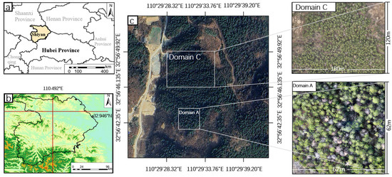
The primary study area was located in a densely forested mountainous region of Shiyan, Hubei Province, central China. The mapped orthomosaic extended from 110°29′28.32″ E to 110°29′41.25″ E and from 32°56′7.01″ N to 32°56′49.92″ N. The area contained continuous canopy cover, overlapping crowns, canopy gaps, shadowed crown surfaces, understory vegetation, dead stems, and locally exposed ground. These features produced marked spatial variation in crown appearance, spectral response, relative thermal intensity, and canopy-surface elevation. Domain C, covering approximately 180 m × 120 m, and Domain A, covering approximately 62 m × 62 m, were identified within the primary study area. Domain A included tree tops, shallow canopy, dark upper canopy, understory areas, and exposed surfaces. The location of the primary study area and the spatial extents of Domain A and Domain C are shown in Figure 1.

Figure 1. Study area and analysis domains in Shiyan, Hubei Province, China. (a) Location of Shiyan within Hubei Province; (b) local topographic context; (c) UAV orthomosaic extent showing Domain A and the representative Domain C; upper right, enlarged Domain C (approximately 180 m × 120 m), used only for the 640 × 640-pixel YOLO11n and FastViT-T8-FPN Faster R-CNN training and model-selection experiments; lower right, enlarged 62 m × 62 m Domain A, within which the separate 416 × 416-pixel standardized evaluation files were defined.

The representative Domain A was selected from a continuous closed-canopy forest with vertically layered and overlapping crowns. Sunlit, shallow-canopy surfaces occupied a large proportion of the visible canopy in Domain A. The high abundance of shallow-canopy reference samples therefore reflected the structural composition of the selected continuous-canopy forest rather than an attempt to balance the six FSZ classes.

2.1.2. Independent Validation Area

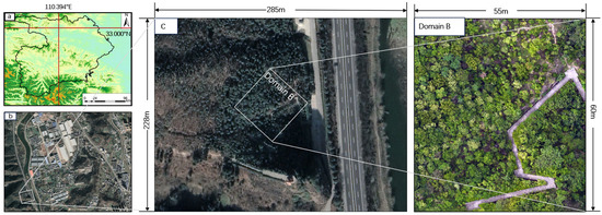
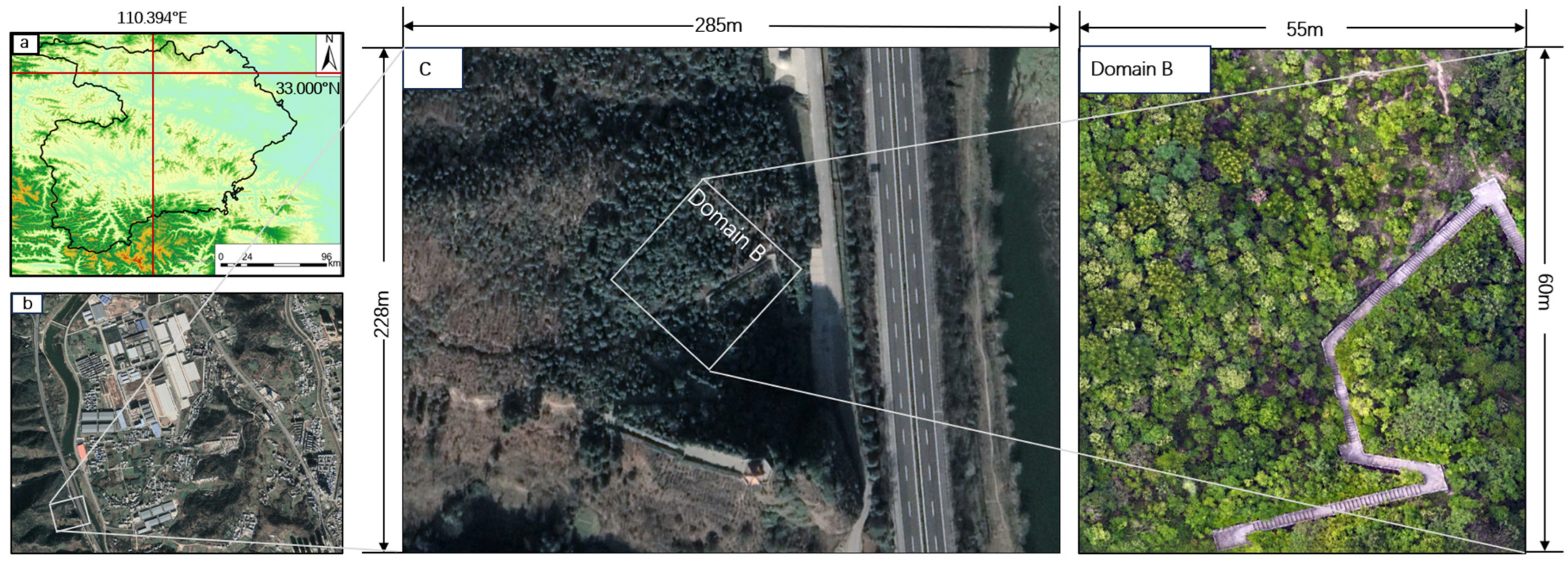
The independent validation area was located in an urban-fringe landscaped scenic area in Shiyan, Hubei Province, central China. The site was spatially separate from the primary mountainous forest area. It extended from 110°23′32.66″ E to 110°23′46.42″ E and from 32°59′54.43″ N to 33°00′04.64″ N, with an approximate extent of 285 m × 228 m.

The area represents a managed urban-green setting dominated by planted trees. It contains a mixture of dense tree cover, canopy gaps, shadowed areas, open ground, and vegetation edges associated with the surrounding scenic landscape. In contrast to the naturally regenerated and densely forested primary study area, the independent area is characterized by more structured vegetation arrangement and stronger influence from adjacent urban infrastructure. The inclusion of this site broadens the study context from a mountainous forest environment to an urban-fringe planted landscape. The location of the independent validation area and the spatial extents of Domain B are shown in Figure 2c.

Figure 2. Independent validation area in Shiyan, Hubei Province, China: (a) location of Shiyan within Hubei Province; (b) local satellite context and outline of the study area; (c) high-resolution imagery of urban-fringe landscaped area, with Domain B delineated; right, enlarged Domain B, a planted-tree area used for independent FSZ validation.

2.2. Research Framework

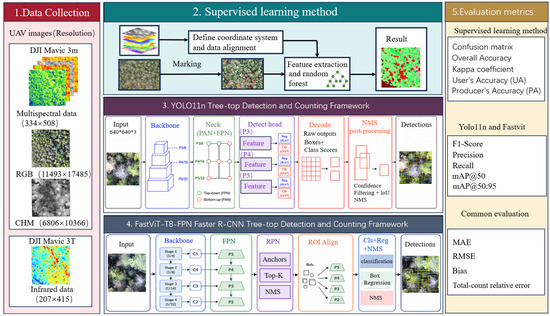
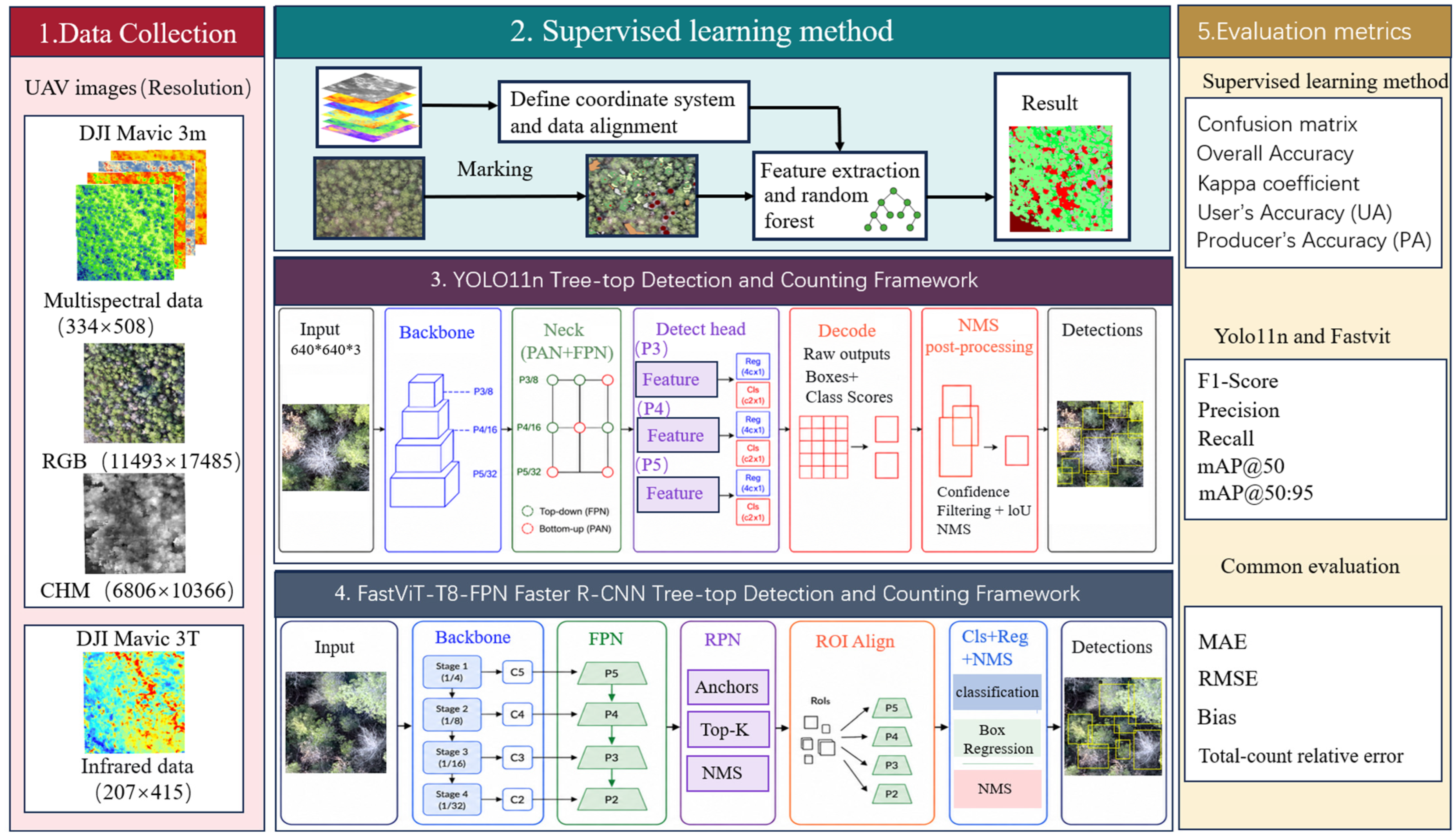
The research framework combined UAV data preparation, six-zone FSZ map generation, tree-top counting, and accuracy evaluation. The FSZ-map workflow used co-registered multispectral, thermal-infrared and CHM layers; YOLO11n and FastViT-T8-FPN Faster R-CNN served as RGB object-detection baselines [33]. Figure 3 presents the research framework.

Figure 3. Research framework for UAV data collection, geospatial multilayer supervised classification, YOLO11n detection, FastViT-T8-FPN Faster R-CNN detection, and the corresponding accuracy evaluation.

2.3. Data Sources and Preprocessing

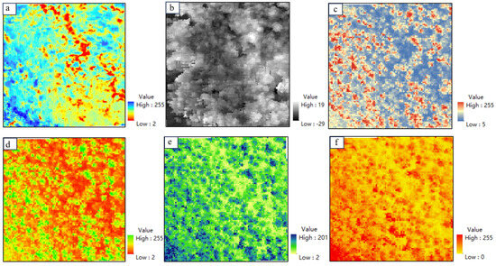
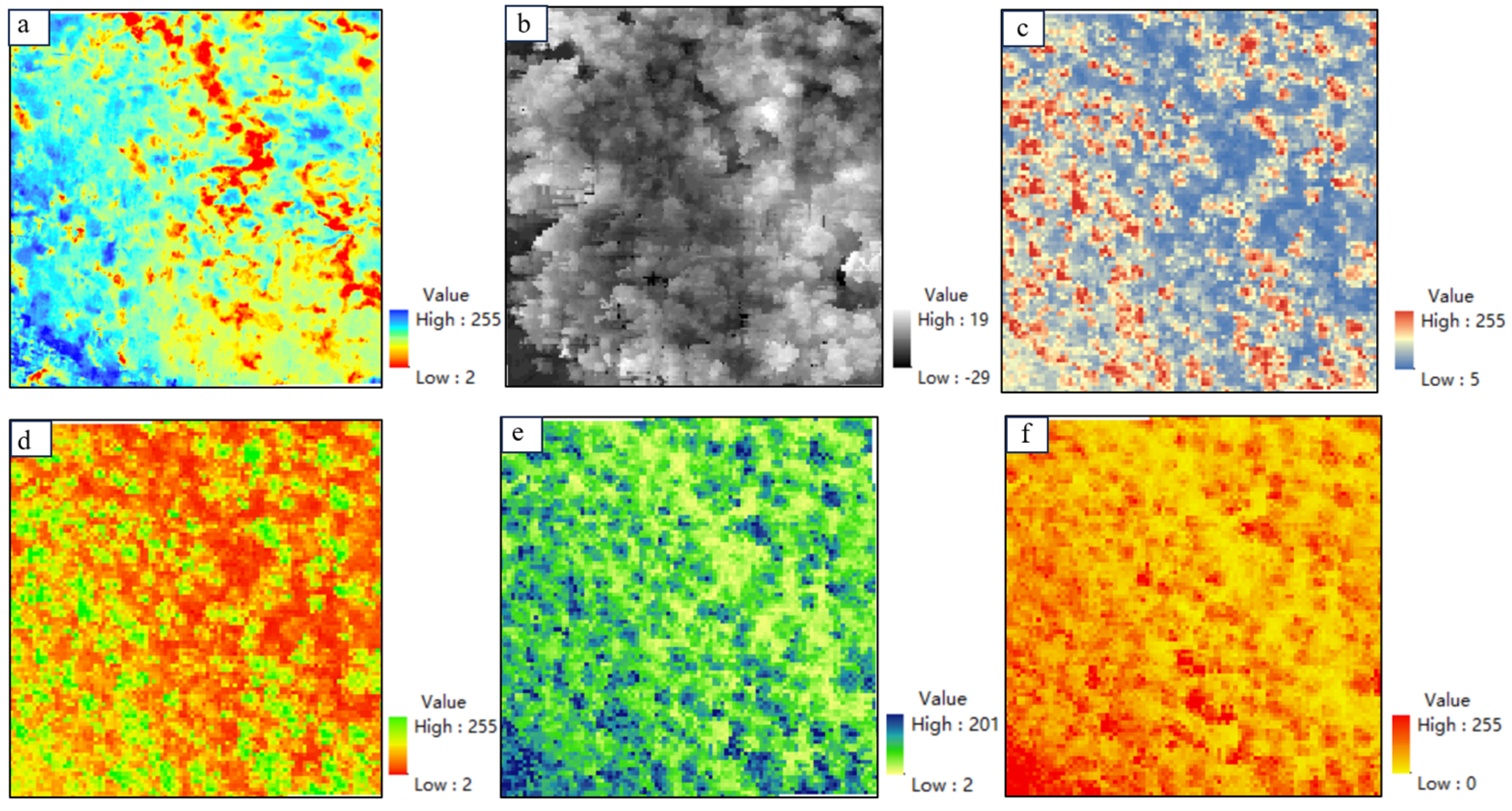
A DJI Mavic 3M UAV acquired RGB and four-band multispectral imagery (green, red, red-edge, and near-infrared; Figure 4c–f). A DJI Mavic 3T UAV acquired thermal-infrared imagery (Figure 4a). The surveys were conducted on 5 February 2026 at approximately 16:00 local time and 40 m above ground level under clear, cloud-free conditions, using the DJI default settings of 80% forward overlap and 70% side overlap. The RGB and processed thermal-infrared orthomosaics had approximate spatial resolutions of 2.4 and 8.37 cm, respectively. DJI Terra V5.2.8 performed image alignment, aerial triangulation, dense reconstruction, and orthomosaic generation separately for the multispectral and thermal-infrared datasets. The thermal layer was represented as a scene-specific stretch of relative radiation intensity, not calibrated surface temperature, and its within-scene contrast supported FSZ discrimination. February acquisition may have influenced crown appearance and class separability. The thermal-infrared layer was represented by a scene-specific color stretch of relative radiation intensity. Its pixel values did not represent absolute or calibrated surface temperatures. Nevertheless, within-scene contrast in relative radiation intensity retained spatial information useful for distinguishing forest structural zones. Image overlap across the study area was sufficient for photogrammetric reconstruction and orthomosaic generation [34].

Figure 4. Representative input layers used for geospatial multilayer supervised classification at a standardized study-area location. (a) Thermal-infrared visualization based on a scene-specific stretch of relative radiation intensity without temperature values; (b) canopy height model (CHM); (c) near-infrared (NIR); (d) red-edge (RE); (e) green (G); and (f) red (R).

The multispectral and thermal-infrared image sets were processed separately through aerial triangulation and orthorectification. A canopy-height CHM was generated during photogrammetric processing to characterize the vertical structure of the forest canopy (Figure 4b). In the present analysis, the DSM and DEM were generated from the same UAV imagery through photogrammetric processing in DJI Terra. The DSM represented the reconstructed canopy surface, whereas the DEM represented the estimated ground surface. The CHM was calculated as DSM − DEM to characterize canopy height relative to the local ground surface [34,35,36]. No external elevation data were used. Figure 4 illustrates the six classification input layers at a standardized study-area location. All outputs were clipped to an analysis extent, co-registered in the GCS_WGS_1984 geographic coordinate system and resampled to a raster geometry. The standardized grid had a cell size of 0.000006° (132 columns × 136 rows in the representative grid shown in Figure 4). The 132 × 136-cell grid represents a representative preprocessing extent rather than the 62 m × 62 m Domain A used for standardized evaluation. The standardized evaluation tiles were defined separately in image-space coordinates. The resulting feature stack comprised green, red, red-edge, near-infrared, relative thermal-infrared and CHM layers for geospatial multilayer supervised classification [35,36]. The RGB orthomosaic was retained separately as the standardized source for the two object-detection workflows. Two raster representations were used at different stages of the workflow. The 0.000006° grid described above was the georeferenced classification grid used for multisource feature alignment, Random Forest classification, and calculation of forest structural-zone coverage. For subsequent tree-top component extraction and count evaluation, the corresponding FSZ output was represented in the pixel geometry of the Domain A image. Therefore, pixel-based spatial parameters used during tree-top post-processing refer to image-space pixels and are independent of the 0.000006° geographic classification grid [37].

The representative Domain A was partitioned a priori into 51 training tiles, four model-selection tiles, and nine 416 × 416-pixel final evaluation tiles. No spatial overlap occurred among the three partitions. The final evaluation tiles were excluded from detector training, checkpoint and threshold selection, and FSZ spatial-parameter selection. All model and post-processing settings were fixed using the training and model-selection partitions before final evaluation. Reference tree-top annotations for the final evaluation tiles were fixed before inference and used only for the final count comparison.

2.4. Tree-Counting Methods

The three workflows estimated tree-top abundance from the same UAV survey. The FSZ-map workflow treated tree counting as a geospatial multilayer supervised-classification and component-extraction task. By contrast, YOLO11n and FastViT-T8-FPN Faster R-CNN treated each tree top as an image object. In every workflow, the predicted count equaled the number of retained tree-top components or detections after spatial post-processing. Counting quality, therefore, depended on identifying individual tree tops while avoiding split or merged crown predictions.

UAV-based tree-top extraction includes pixel-based classification, semantic segmentation, instance segmentation, object detection, and LiDAR-based crown segmentation. Pixel-based classification and semantic-segmentation models generate wall-to-wall class maps. Instance-segmentation models separate individual crown instances. Object detectors predict discrete tree-top locations or bounding boxes. LiDAR-based methods use point-cloud structure or canopy-height models to identify tree tops and crown boundaries [38,39]. This study used Random Forest pixel-based FSZ classification to generate a continuous forest structural map from co-registered multispectral, relative thermal-infrared, and CHM layers. The training data consisted of polygon labels for six FSZ classes. The FSZ map provided the input for subsequent tree-top component extraction. This workflow matched the available training labels and the wall-to-wall structural characterization objective [40,41].

2.4.1. A Proposed FSZ-Based Framework for Tree-Top Counting While Preserving Structural Context

(1)

Overall FSZ-Based Tree-Top Counting Framework

This study proposed an FSZ-based framework that first generated a wall-to-wall forest structural zone map, and then extracted tree-top candidates through spatial post-processing. The framework preserved the structural context of tree tops rather than treating them as isolated two-dimensional land-cover objects. Ultra-high-resolution multisource UAV data represented the forest as a complex 2.5D surface, and the classification logic integrated object type, illumination, canopy structure, and local height variation.

The base FSZ map contained six structural classes: tree tops (class 1), dead tree trunks (class 2), shallow canopy (class 3), dark upper canopy (class 4), understory area (class 5), and exposed surface (class 6). Tree-top labels referred only to localized visible crown-apex regions representing a distinct local maximum or visually identifiable crown center, whereas shallow-canopy labels represented surrounding illuminated upper-crown surfaces without a distinct apex. Ambiguous apex-to-canopy transitions were delineated conservatively according to the local crown-center criterion.

The same framework was extended to an urban-fringe landscape containing houses, roads, and other artificial surfaces. The local six-class scheme comprised tree tops, shallow canopy, dark canopy, understory shadow, exposed ground, and artificial surface. The Random Forest classification settings were kept identical to those used in the primary forest experiment. Only the spatial post-processing parameters used to convert the FSZ map into final tree-top counts were calibrated separately for the urban-fringe site.

(2)

Initial Calibration of the Six-Class FSZ Map

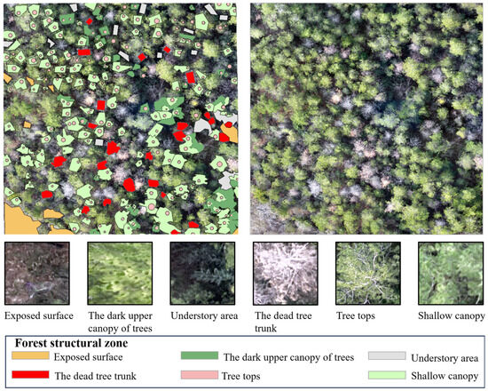
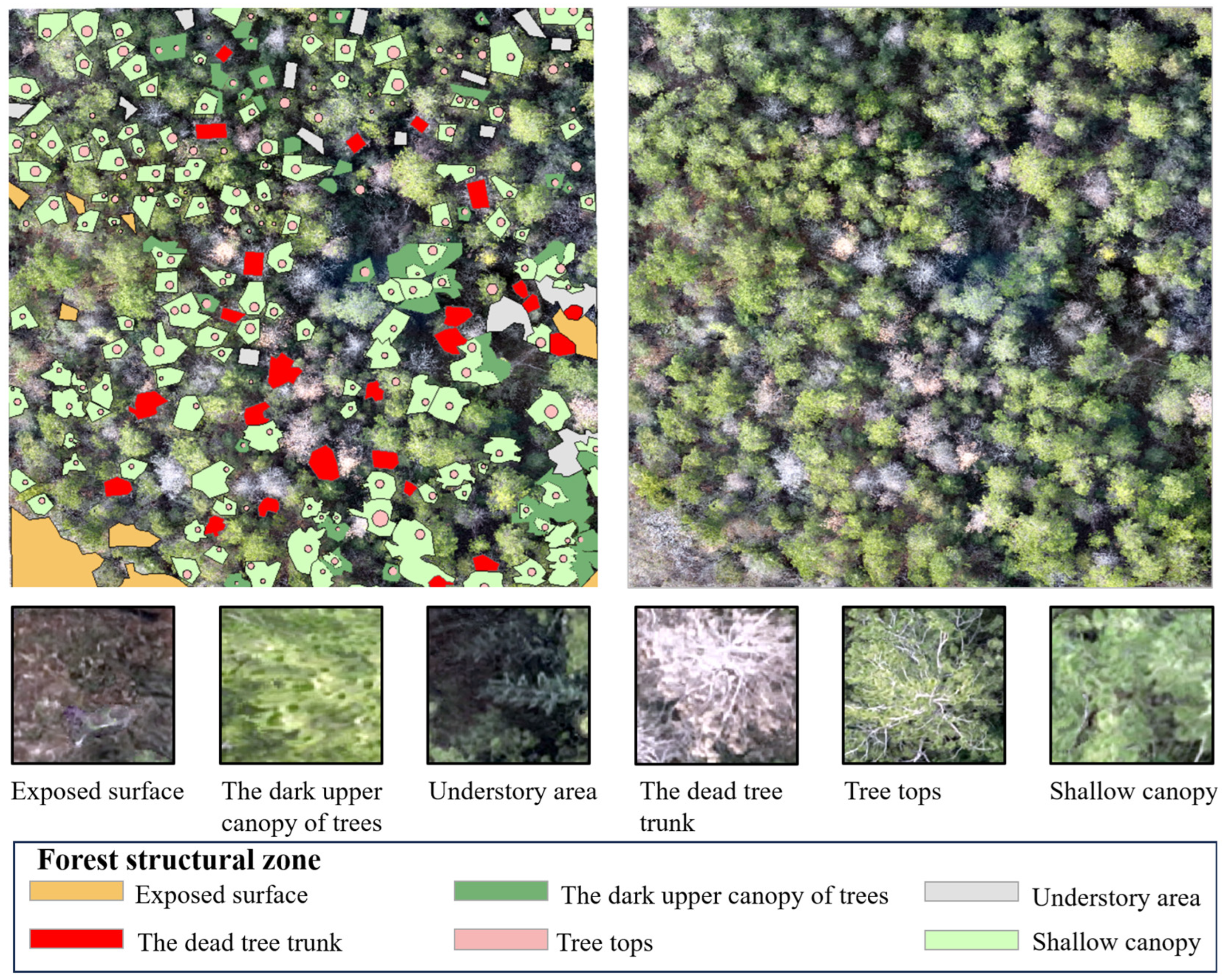
Representative domains were delineated by expert visual interpretation in ArcMap 10.8 and assigned to the six base FSZ classes. The training KMZ contained 418 labeled polygons: 195 tree-top, 25 dead-tree-trunk, 133 shallow-canopy, 42 dark-upper-canopy, 15 understory, and 8 exposed-surface polygons. These counts represent labeled regions rather than raster pixels; pixels within the polygons served as class-specific training samples. The labeled domains and visual examples of the six reference structural zones are shown in Figure 5.

Figure 5. Representative Domain A and six reference forest structural zones used for geospatial multilayer supervised classification. Left, polygon-based training labels overlaid on the RGB orthomosaic; right, the corresponding unlabeled RGB image; bottom, visual examples of each zone.

The classification workflow was organized in ArcMap 10.8, and the base FSZ classifier was implemented using the Local Climate Zone Classification tool chain in SAGA GIS 5.0.0, which calls Random Forest Classification (ViGrA). The aligned green, red, red-edge, near-infrared, relative thermal-infrared, and CHM layers were used as input features. The Source field served as the class-label field, Use Label as Identifier was set to true, and minimum redundancy feature selection was disabled. The Random Forest used 32 trees, all available training samples per tree with replacement, a minimum node split size of 1, the square-root option for feature number per node, no stratification, and no optional probability or feature-importance outputs. The classifier assigned one FSZ label to each orthomosaic cell.

A_i = N_i × A_cell

(1)

where N_i is the number of raster cells classified as zone i, and A_cell is the ground area of one cell.

(3)

Secondary FSZ-Based Tree-Top Extraction and Counting

After the six-zone base FSZ map was produced, class 1 was used as the primary source of living tree-top candidates. Conservative spatial filtering suppressed isolated noise cells and improved local continuity, after which connected candidate cells were grouped into components. Candidate extraction was conducted in the pixel geometry of the corresponding Domain A image. Class 2 components were processed separately through a secondary branch dedicated to dead-tree-top extraction. After component filtering, peak-based splitting, and spatial non-maximum suppression relative to the retained Class 1 candidates, qualified Class 2 components were subsequently relabeled as Class 7 dead-tree-top candidates. Class 7 was excluded from the six-class confusion-matrix and zone-accuracy assessments and was considered only in the final end-to-end tree-top counting output.

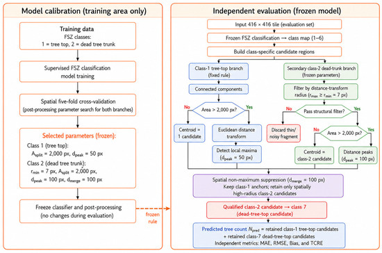
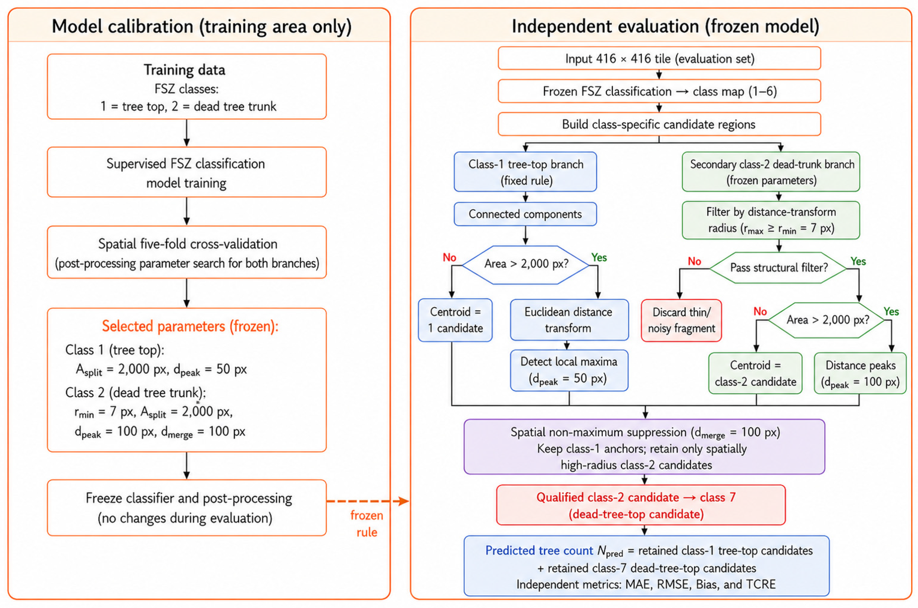
The 51 annotated training tiles, together with their KMZ-derived semantic polygons and base FSZ maps, were used only to tune spatial post-processing parameters. No tile-level regression model was used; counts were obtained directly from retained components after candidate extraction, connected-component analysis, and peak-based splitting of oversized components. Both candidate branches’ post-processing parameters were tuned via spatial five-fold cross-validation to minimize absolute TCRE. Class 1 selected Asplit = 2000 pixels and dpeak = 50 pixels; Class 2 selected rmin = 7 pixels, Asplit = 2000 pixels, dpeak = 100 pixels, and dmerge = 100 pixels (Figure 6). All were fixed before the final evaluation. The finalized workflow was applied once to nine spatially independent 416 × 416-pixel evaluation tiles containing 77 reference tree tops, following the training-only parameter-tuning and independent-evaluation structure summarized in Figure 6. For the urban-fringe implementation, tree-top extraction parameters were calibrated only on the urban-fringe training partition using four-fold spatial cross-validation; the final configuration used a 0.18 tree-top score threshold, a 1.5 FSZ-cell matching tolerance, and a 4.0 FSZ-cell inter-peak spacing, approximately 2.19 m.

Figure 6. Training-only spatial-parameter tuning and independent evaluation of the FSZ map tree-counting workflow.

2.4.2. YOLO11n Tree-Top Counting

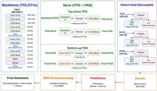
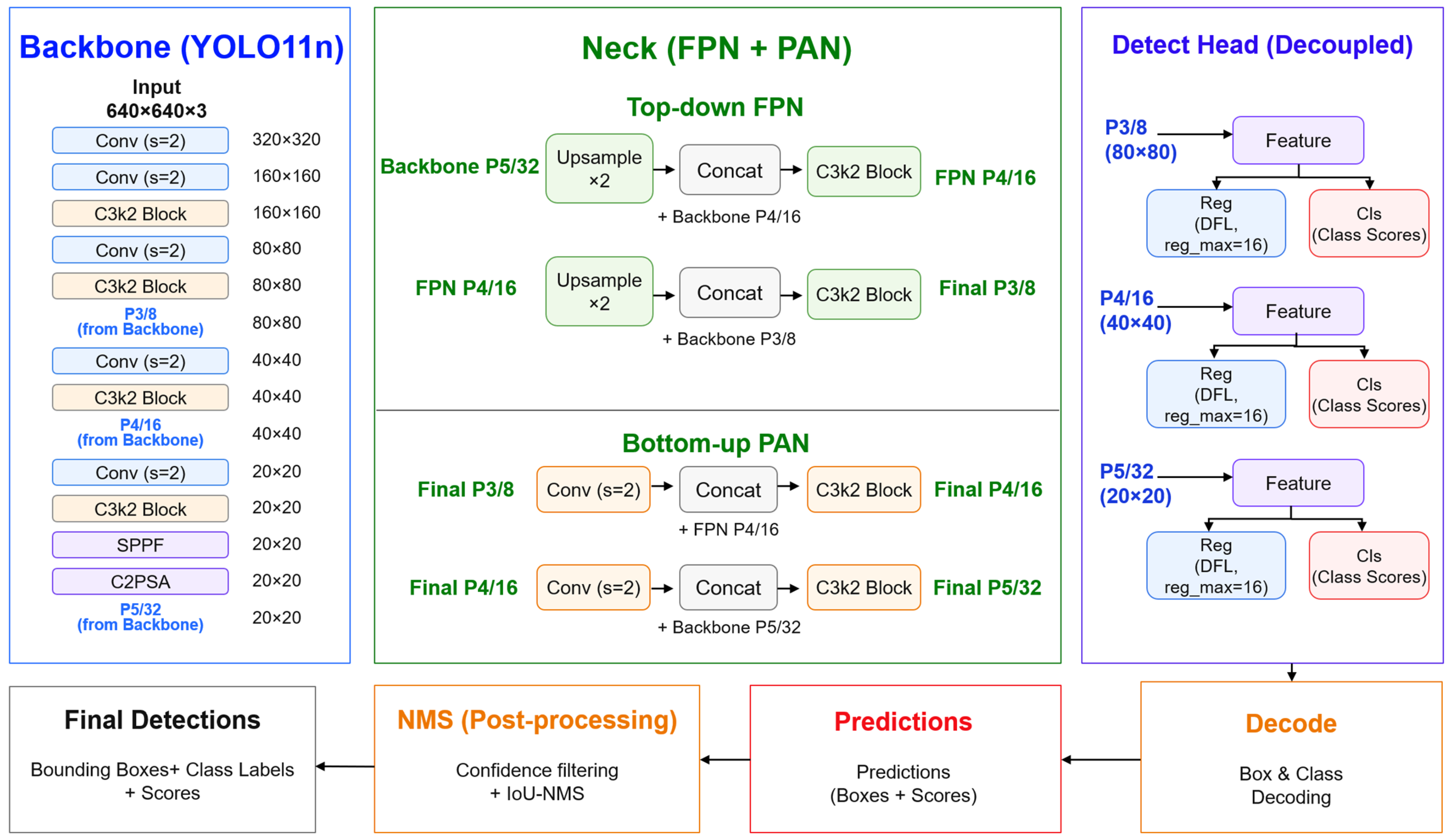
YOLO11n was implemented for tree-top recognition using Python 3.12.7, PyTorch 2.14.0.dev20260802+cu130, and Ultralytics 8.4.115. The conceptual end-to-end detection workflow of the model is illustrated in Figure 7. The nano-scale model was initialized with the pretrained YOLO11n weights for single-class tree detection. This model comprised 101 layers, 2,582,347 parameters, and 6.4 GFLOPs. Domain C (Figure 1) supplied the RGB orthomosaic, subdivided into fixed 640 × 640-pixel tiles and annotated with bounding boxes for discernible tree tops. This initial experiment comprised 314 training images and 74 spatially independent validation images. The Domain C experiment was separate from the standardized evaluation, which used independent 416 × 416-pixel files in Domain A (Section 3.3). During inference, YOLO11n generated a bounding box and confidence score for each candidate tree top per tile [42,43].

Figure 7. Conceptual end-to-end detection workflow used to contextualize YOLO11n tree-top detection, illustrating image tiling, feature extraction, multiscale fusion and bounding-box prediction.

For the standardized evaluation run, 416 × 416-pixel image tiles were partitioned into 51 training tiles, four model-selection tiles, and nine final independent evaluation tiles. Training ran for a maximum of 100 epochs with early stopping (patience = 30), stopping at epoch 66. AdamW was used with a batch size of 8 and an initial learning rate of 0.001. A cosine learning-rate schedule (cos_lr = True) was applied with three warm-up epochs and a final learning-rate fraction of 0.01. The optimal model checkpoint from epoch 36 was retained because it achieved the highest validation mAP@50:95 on the four model-selection tiles. Training used a fixed random seed of 42 and deterministic execution on an NVIDIA GeForce RTX 5070 Laptop GPU (8151 MiB) under CUDA 13.0. Data augmentation included HSV adjustments (hue = 0.015, saturation = 0.7, value = 0.4), translation (0.1), scaling (0.5), horizontal flipping (p = 0.5), mosaic augmentation (p = 1.0), RandAugment (default settings), and random erasing (p = 0.4). Rotation, shear, perspective transformation, vertical flipping, MixUp, CutMix, and Copy-Paste were not applied. The final nine-tile evaluation was run once with a confidence threshold of 0.50 and a non-maximum-suppression IoU threshold of 0.70. Detected boxes were transformed from tile coordinates to orthomosaic coordinates, and detections from overlapping or adjacent tiles were reconciled before counts were calculated. The final independent evaluation set was not used for training, checkpoint selection, or threshold selection [44,45].

2.4.3. FastViT-T8-FPN Faster R-CNN Tree-Top Counting

FastViT-T8-FPN Faster R-CNN was implemented as a two-stage RGB object detector.

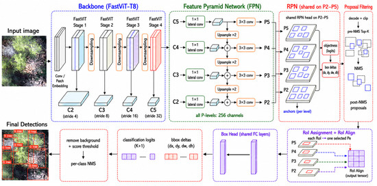
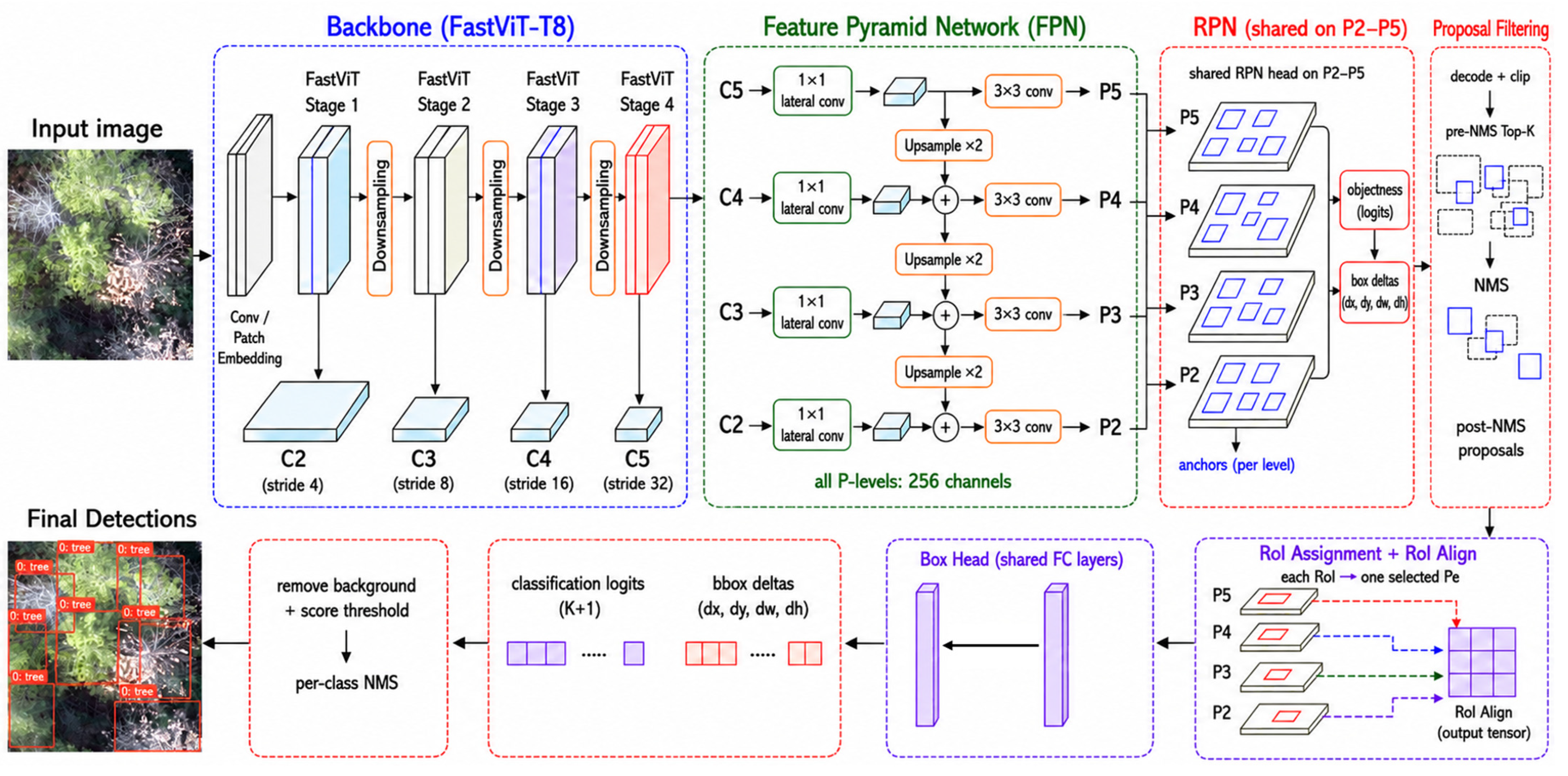
The conceptual end-to-end detection workflow of the model is illustrated in Figure 8. The FastViT-T8 backbone was trained from random initialization without pretrained weights. FastViT-T8-FPN Faster R-CNN was trained and evaluated in the same computing environment as YOLO11n, using Python 3.12.7, PyTorch 2.14.0.dev20260802+cu130, and CUDA 13.0 on an NVIDIA GeForce RTX 5070 Laptop GPU. Input images were resized to 416 × 416 pixels. Training used AdamW with a batch size of 8, an initial learning rate of 0.001, a cosine learning-rate schedule, three warm-up epochs, and early stopping with a patience of 30 epochs. The same data-augmentation strategy, random seed of 42, and deterministic execution described in Section 2.4.2 were used. The checkpoint with the highest validation mAP@50:95 on the four model-selection tiles was retained. During inference, the confidence threshold was 0.50 and the non-maximum-suppression IoU threshold was 0.70. A FastViT-T8 backbone extracted hierarchical image features, which were integrated through a feature pyramid network. The resulting features were passed to the region-proposal and bounding-box refinement stages of Faster R-CNN. The model used the same Domain C 640 × 640-pixel RGB tile-based annotation framework as YOLO11n for its initial training and model-selection experiment, with tree tops defined as the target object class [42,46]. The later standardized evaluation used the separate 416 × 416-pixel Domain A files described in Section 3.3.

Figure 8. FastViT-T8-FPN Faster R-CNN workflow for tree-top detection. The architecture combines hierarchical feature extraction by the FastViT-T8 backbone, multiscale feature fusion by the FPN, and two-stage proposal refinement by Faster R-CNN to detect individual tree tops in dense, heterogeneous forest canopies.

The detector generated bounding boxes and confidence scores for candidate tree tops. These detections were projected to the orthomosaic coordinate system and reconciled across tiles using the same counting principle as YOLO11n. The final count was, therefore, the number of unique retained tree-top detections. Despite their different internal architectures, YOLO11n and FastViT-T8-FPN Faster R-CNN both required consistent confidence filtering, tile-overlap handling and duplicate removal before detection outputs could be interpreted as tree counts [47,48].

2.5. Accuracy Evaluation

Evaluation was conducted at two complementary levels. First, each workflow was assessed with metrics appropriate to its native output. The detector-specific metrics reported for YOLO11n and FastViT-T8-FPN Faster R-CNN describe their separate 640 × 640-pixel Domain C initial model-development experiments; the FSZ map was assessed from independent reference samples. Second, all three workflows were compared through tree-top counts within nine matched 416 × 416-pixel files defined in the shared Domain A. These files were spatially independent of the initial Domain C experiments. For the YOLO11n standardized evaluation run, separate 51-tile training and four-tile model-selection partitions were also held apart from the final nine-tile evaluation partition. This design prevents FSZ-map and bounding-box detection scores from being conflated, while directly testing the practical objective of accurate tree-top enumeration. To enable a comparable operational assessment of tree-count estimates across the three workflows, we used a common count-level endpoint. Because the FSZ workflow and RGB object detectors differed in input data, intermediate outputs, and extraction mechanisms, this endpoint compared operational outputs rather than analytically equivalent models.

2.5.1. Evaluation of the FSZ Map

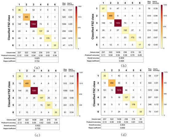
The six-zone base FSZ map was evaluated with a confusion matrix derived from independent reference samples (Figure 9). An expert-based reference-sampling design was used. A botanist selected 2707 independent reference samples through visual interpretation of the co-registered UAV imagery and CHM. These samples were selected independently of the 418 labeled training polygons and were used only for accuracy assessment. Sample allocation was not constrained to be equal among the six FSZ classes. The classwise reference sample totals are reported in the confusion matrices in Figure 9. The higher representation of shallow-canopy samples reflects the structural composition of the selected continuous-canopy Domain A rather than an imposed balanced sampling design. For zone i, n_ii is the number of correctly classified samples, r_i is the predicted total and c_i is the reference total. N is the total sample size, K = 6, and p_e is the expected agreement calculated from the row and column totals. Overall accuracy (OA), kappa (κ), zone-specific user’s accuracy (UA), producer’s accuracy (PA), F1 score and macro F1 were calculated using Equations (2)–(5). UA reflects commission error and PA reflects omission error.

$$OA={\displaystyle \frac{1}{N}}{\displaystyle {\sum }_{i=1}^K}{n}_{ii}$$

(2)

$$\kappa ={\displaystyle \frac{p_o-p_e}{1-p_e}}, p_o=OA, p_e={\displaystyle \frac{1}{N^2}}{\displaystyle {\sum }_{i=1}^K}{r}_i{c}_i$$

(3)

$${UA}_i={\displaystyle \frac{n_{ii}}{r_i}}, {PA}_i={\displaystyle \frac{n_{ii}}{c_i}}$$

(4)

$${F1}_i={\displaystyle \frac{2\left({UA}_i\times {PA}_i\right)}{{UA}_i+{PA}_i}}, Macro F1={\displaystyle \frac{1}{K}}{\displaystyle {\sum }_{i=1}^K}{F1}_i$$

(5)

Figure 9. Confusion matrices for the pixel-level FSZ input-ablation analysis in the primary experiment area. Rows denote classified FSZ classes, and columns denote reference FSZ classes. (a) Multispectral + relative thermal infrared + CHM; (b) multispectral + CHM, without relative thermal infrared; (c) multispectral + relative thermal infrared, without CHM; and (d) relative thermal infrared + CHM, without multispectral bands.

Macro F1 was calculated as the unweighted mean of the six classwise F1 scores. Because tree counting was the principal application, map accuracy alone was insufficient. The tree-top zone was, therefore, also evaluated after connected-component extraction. For each evaluation file, the number of retained components was compared with the reference tree-top count. This analysis tested whether pixel-level accuracy translated into reliable tree counts and identified over-segmentation, under-segmentation and missed tree-top components.

Balanced accuracy was calculated as the macro-average of producer’s accuracy across the six FSZ classes. This metric assigns equal weight to each class and complements overall accuracy under the uneven class distribution of the continuous-canopy Domain A. All pixel-level FSZ map-accuracy metrics reported in this section refer exclusively to Classes 1–6; Class 7 was evaluated only as part of the final post-processed tree-top extraction output.

2.5.2. Input Ablation Analysis of the FSZ Classification

Input ablation was conducted in Domain A to quantify the contributions of multispectral, relative thermal-infrared, and canopy-height information to six-zone FSZ classification. Independent of the standardized tree-top count evaluation, this analysis focused on pixel-level FSZ mapping, with the four evaluated feature stacks summarized in Table 1. The full configuration contained green, red, red-edge, near-infrared, relative thermal-infrared, and canopy height model (CHM) layers; three component-removal configurations were constructed by sequentially removing the relative thermal-infrared layer, the CHM, or all multispectral bands, resulting in multispectral + CHM, multispectral + relative thermal infrared, and relative thermal infrared + CHM stacks, respectively [49,50]. All configurations shared identical settings (418 labeled training polygons, six FSZ classes, raster extent, spatial resolution, and Random Forest parameters) to produce six-zone base maps. Using the same independent reference samples and confusion-matrix procedures, overall accuracy, Cohen’s kappa coefficient, class-specific user’s accuracy, producer’s accuracy, F1 score, and macro-F1 score were calculated, with tree-top F1 employed to evaluate discrimination between tree tops and canopy classes. To focus on the effects of input composition, the analysis excluded connected-component extraction, spatial filtering, peak-based splitting, and tree-count calculation, thereby describing pixel-level FSZ classification performance.

Table 1. Input-ablation feature stacks for six-zone FSZ classification in Domain A.

Configuration	Multispectral Bands	Relative Thermal-Infrared	CHM	Removed Component
Full feature stack	Included	Included	Included	None
Without relative thermal infrared	Included	Excluded	Included	Relative thermal infrared
Without CHM	Included	Included	Excluded	CHM
Without multispectral bands	Excluded	Included	Included	All multispectral bands

2.5.3. Evaluation of YOLO11n and FastViT-T8-FPN Faster R-CNN

The detector-specific results for the initial 640 × 640-pixel Domain C experiments were calculated using the reference boxes and a one-to-one matching rule. At an intersection-over-union (IoU) threshold of 0.50, a predicted box that matched one reference tree-top box was counted as a true positive (TP). Unmatched predicted boxes were counted as false positives (FPs), whereas unmatched reference boxes were counted as false negatives (FNs). Precision, recall, and F1 score were calculated using Equations (6) and (7), while average precision (AP) and mAP were calculated using Equations (8) and (9). The independent 416 × 416-pixel evaluation is reported separately as a count-level comparison in Section 3.3.

$$Precision={\displaystyle \frac{TP}{TP+FP}}, Recall={\displaystyle \frac{TP}{TP+FN}}$$

(6)

$$F1={\displaystyle \frac{2\left(Precision\times Recall\right)}{Precision+Recall}}$$

(7)

$${AP}_t={\displaystyle {\int }_0^1}P\left(R\right)dR$$

(8)

$$mAP@50={AP}_{0.50}, mAP@50:95={\displaystyle \frac{1}{10}}{\displaystyle {\sum }_{s=0}^9}{AP}_{0.50+0.05s}$$

(9)

Average precision (AP) was the area under the interpolated precision–recall curve at IoU threshold t. For the single tree-top zone, mAP@50 corresponded to AP at IoU = 0.50. mAP@50:95 was the mean AP across ten thresholds from 0.50 to 0.95 in increments of 0.05. For the separate standardized count evaluation, the post-processed number of retained detections in each final independent 416 × 416-pixel tile was compared with the reference count. This analysis was necessary because a detector can achieve an acceptable box-matching score yet still bias the total count through duplicate detections, missed tree tops at tile boundaries or confidence-threshold effects.

2.5.4. Standardized Evaluation of Accuracy Across FSZ, YOLO, and ViT

For each evaluation file i, count error was defined as e_i = Npred_i − Nref_i. Absolute error quantified the magnitude of error, whereas signed error indicated systematic overcounting or undercounting. Across M evaluation files, MAE, RMSE, mean bias error (bias) and total-count relative error (TCRE) were calculated using Equations (10)–(14).

$$e_i={Npred}_i-{Nref}_i, {AE}_i=\left|e_i\right|$$

(10)

$$MAE={\displaystyle \frac{1}{M}}{\displaystyle {\sum }_{i=1}^M}\left|e_i\right|$$

(11)

$$RMSE=\sqrt{{\displaystyle \frac{1}{M}}{\displaystyle {\sum }_{i=1}^M}{e_i}^2}$$

(12)

$$Bias={\displaystyle \frac{1}{M}}{\displaystyle {\sum }_{i=1}^M}{e}_i$$

(13)

$$TCRE={\displaystyle \frac{{\displaystyle {\sum }_{i=1}^M}{Npred}_i-{\displaystyle {\sum }_{i=1}^M}{Nref}_i}{{\displaystyle {\sum }_{i=1}^M}{Nref}_i}}\times 100\mathrm{\%}$$

(14)

Lower MAE and RMSE indicated more accurate and stable tree-top counts. Bias and TCRE values closer to zero indicated less systematic overcounting or undercounting. The standardized count-level analysis complemented the native classification and detection metrics. It provided a shared, management-relevant assessment of whether each workflow produced a usable estimate of tree abundance. Native metrics were retained to identify whether counting errors arose from class confusion, missed detections, duplicate detections or inaccurate localization.

Paired nonparametric bootstrap resampling was used to quantify uncertainty in the standardized count comparison. The nine evaluation tiles were resampled with replacement 10,000 times while preserving the paired reference and predicted counts for each workflow. Percentile-based 95% confidence intervals were calculated for MAE, RMSE, bias, TCRE, and pairwise differences in MAE, RMSE, and absolute TCRE. A pairwise difference was not interpreted as evidence of a performance difference when its 95% confidence interval included zero.

2.5.5. Independent Validation of FSZ Classification and Tree-Top Extraction

A new six-class FSZ classifier was trained using the urban-fringe training partition, while retaining the same six input layers and Random Forest hyperparameters as in Domain A. Only the final tree-top extraction parameters were calibrated on the urban-fringe training partition before evaluation of the held-out subset.

Evaluation proceeded at two levels: first, a six-zone confusion matrix was assessed on independent reference samples to measure raw pixel-level classification, yielding overall accuracy, Cohen’s kappa, user’s/producer’s accuracy, F1, and macro-F1. Second, final tree tops were matched to annotated reference tree tops using a 1.5 FSZ-unit (approx. 0.83 m) one-to-one spatial tolerance, recording true/false positives and negatives. User’s accuracy, producer’s accuracy, and F1 (UA = TP/(TP + FP), PA = TP/(TP + FN), F1 = 2TP/(2TP + FP + FN)) were computed along with the total-count relative error.

3. Results

3.1. Accuracy and Input Ablation of the Six-Zone FSZ Map

Figure 9 compares four input configurations using the same 2707 independent reference samples. The full multispectral, relative thermal-infrared, and CHM stack achieved an overall accuracy of 0.825, a kappa coefficient of 0.724, a macro-F1 score of 0.709, and a balanced accuracy of 0.730 (Figure 9a). Class-specific results are reported in Table 2.

Table 2. Zone-specific accuracy of the six-zone FSZ map produced by the full multispectral + relative thermal infrared + CHM configuration in the primary experiment area. Balanced accuracy was 0.730, calculated as the macro-average of producer’s accuracy across the six classes.

FSZ Class	Structural Zone	User’s Accuracy	Producer’s Accuracy	F1 Score
1	Tree tops	0.41	0.15	0.22
2	Dead tree trunk	0.95	0.95	0.95
3	Shallow canopy	0.85	0.94	0.89
4	Dark upper canopy	0.66	0.58	0.62
5	Understory area	0.73	0.82	0.77
6	Exposed surface	0.70	0.94	0.80

The full feature stack accurately classified dead tree trunks and shallow canopy. Tree tops had the lowest producer’s accuracy, with a user’s accuracy of 0.41, a producer’s accuracy of 0.15, and an F1 score of 0.217. Among 257 reference tree-top samples, 142 were classified as shallow canopy. Removing relative thermal infrared reduced overall accuracy to 0.809, macro-F1 to 0.625, and tree-top F1 to 0.161 (Figure 9b). The exposed-surface F1 score decreased from 0.805 to 0.442. The no-CHM configuration produced similar scores to the full stack, with an overall accuracy of 0.822, a kappa coefficient of 0.720, a macro-F1 score of 0.690, and a tree-top F1 score of 0.201 (Figure 9c). Removing multispectral bands produced the lowest overall accuracy (0.804) and kappa coefficient (0.692), with a macro-F1 score of 0.654 and a tree-top F1 score of 0.154 (Figure 9d). Tree-top pixels were consistently confused with shallow canopy across all configurations.

3.2. Detection Performance of YOLO11n and FastViT-T8-FPN Faster R-CNN

In the initial 640 × 640-pixel Domain C detector assessment, YOLO11n achieved a precision of 0.652, recall of 0.779 and F1 score of 0.710 at IoU = 0.50. Its mAP@50 and mAP@50:95 were 0.753 and 0.272, respectively (Table 3). FastViT-T8-FPN Faster R-CNN achieved a precision of 0.823, recall of 0.662 and F1 score of 0.734, with mAP@50 of 0.749 and mAP@50:95 of 0.240. Thus, FastViT-T8-FPN Faster R-CNN yielded higher precision and F1 score, whereas YOLO11n yielded higher recall and mAP@50:95. These native detector metrics are distinct from the final 416 × 416-pixel independent count evaluation reported below.

Table 3. Detection accuracy of the two RGB object detectors in the initial 640 × 640-pixel Domain C model-development assessments.

Method	Precision	Recall	F1 Score	mAP@50	mAP@50:95
YOLO11n	0.652	0.779	0.710	0.753	0.272
FastViT-T8-FPN Faster R-CNN	0.823	0.662	0.734	0.749	0.240

3.3. Standardized Evaluation of Tree Counts

The independent standardized count comparison comprised nine spatially independent 416 × 416-pixel Domain A files containing 77 reference tree tops (Table 4). These files were separate from the 640 × 640-pixel Domain C initial detector experiments. For YOLO11n, the 416-pixel run was trained on 51 separate tiles, its epoch-36 checkpoint was selected from four model-selection tiles using mAP@50:95, and the nine standardized evaluation tiles were used only once for final evaluation. Using spatial post-processing parameters selected from the training tiles, the FSZ-map workflow predicted 66 tree tops (MAE, 1.889; RMSE, 2.517; bias, −1.222; total-count relative error, −14.29%). YOLO11n predicted 60 tree tops (MAE, 1.889; RMSE, 2.472; bias, −1.889; total-count relative error, −22.08%). FastViT-T8-FPN Faster R-CNN predicted 62 tree tops (MAE, 1.667; RMSE, 2.236; bias, −1.667; total-count relative error, −19.48%). The observed point estimates differed across the count metrics. MAE and RMSE describe tile-level count error, whereas absolute TCRE describes the difference between summed predicted and reference counts. Paired bootstrap confidence intervals for all pairwise differences in MAE, RMSE, and absolute TCRE included zero (Table 5). Differences were calculated as the metric of the first-listed workflow minus that of the second-listed workflow. All 95% confidence intervals include zero. The nine-tile evaluation, therefore, does not support a definitive ranking among the workflows. These results describe within-site performance under the acquisition conditions of the present survey.

Table 4. Independent standardized tree-counting evaluation across all workflows.

Workflow	Predicted Tree Tops	Reference Tree Tops	MAE (95% CI)	RMSE (95% CI)	Bias (95% CI)	TCRE, % (95% CI)
FSZ workflow	66	77	1.889 (0.778–3.000)	2.517 (1.491–3.333)	−1.222 (−2.667–0.111)	−14.29 (−29.27–1.54)
YOLO11n	60	77	1.889 (0.889–3.000)	2.472 (1.247–3.464)	−1.889 (−3.000–−0.889)	−22.08 (−32.88–−11.27)
FastViT-T8-FPN Faster R-CNN	62	77	1.667 (0.778–2.667)	2.236 (1.247–2.944)	−1.667 (−2.667–−0.778)	−19.48 (−29.63–−8.96)

Table 5. Pairwise bootstrap differences in count-error metrics.

Pairwise Comparison	Difference in MAE (95% CI)	Difference in RMSE (95% CI)	Difference in Absolute TCRE, Percentage Points (95% CI)
FSZ − YOLO11n	0.000 (−1.444–1.444)	0.045 (−1.201–1.472)	−7.792 (−25.676–12.500)
FSZ − FastViT-T8-FPN Faster R-CNN	0.222 (−0.333–0.667)	0.281 (−0.241–0.719)	−5.195 (−14.286–2.899)
YOLO11n − FastViT-T8-FPN Faster R-CNN	0.222 (−1.111–1.556)	0.236 (−0.933–1.294)	2.597 (−13.043–18.667)

Spatial five-fold cross-validation of the 51 training tiles selected A_split = 2000 image-space pixels and a minimum inter-peak distance of 50 image-space pixels, using the smallest absolute TCRE as the parameter-selection criterion. The secondary Class 2 branch was included in the training-only spatial cross-validation for post-processing parameter selection. Qualified Class 2 candidates were relabeled as Class 7 dead-tree tops, and the final FSZ count included retained Class 1 and Class 7 candidates. All selected parameters were frozen before application to the nine final evaluation tiles.

3.4. Independent Validation in the Urban-Fringe Planted Landscape

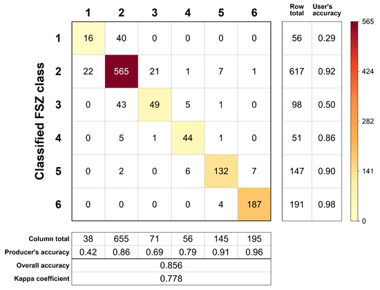
The raw six-zone FSZ classification in the independent validation subset achieved an overall accuracy of 0.856 and a Cohen’s kappa coefficient of 0.778 before spatial post-processing (Figure 10). The macro-F1 score was 0.751. For the tree-top class, the user’s accuracy was 0.286, the producer’s accuracy was 0.421, and the F1 score was 0.340. Sixteen reference tree-top samples were correctly classified. Forty reference shallow-canopy samples (class 2 in the urban FSZ scheme) were classified as tree tops, representing the principal source of tree-top commission error in the raw FSZ map.

Figure 10. Confusion matrix for six-zone FSZ classification before spatial post-processing in the rectangular independent-validation subset of the urban-fringe planted landscape. Rows denote classified FSZ classes and columns denote reference FSZ classes.

After final FSZ spatial processing with a 4.0-unit inter-peak spacing, 38 tree tops were predicted in the independent validation subset, compared with 47 manually annotated reference tree tops. One-to-one matching yielded 24 TP, 14 FP, and 23 FN. The resulting UA, PA, and F1 scores were 63.16%, 51.06%, and 56.47%, respectively (Table 6). The predicted total was nine tree tops lower than the reference total, corresponding to a total-count relative error of −19.15%. The pixel-level classification metrics and tree-top matching metrics are reported separately because they represent different evaluation units.

Table 6. One-to-one matching results for tree-top extraction after final FSZ spatial post-processing with a 4.0-unit inter-peak spacing in the independent validation subset.

Reference Tree Tops	Predicted Tree Tops	TP	FP	FN	UA	PA	F1
47	38	24	14	23	63.16%	51.06%	56.47%

4. Discussion

4.1. Accuracy and Cross-Domain Counting Performance of the Workflows

4.1.1. Interpretation of Class Confusion and Feature Contributions in Domain A

(1)

Mechanistic interpretation and actionable guidance

In the dense, heterogeneous forest of Domain A, tree tops and shallow canopy form a continuous upper-canopy surface. Their similarities in spectral, relative thermal, and height characteristics caused by adjacent crowns, illumination gradients, and CHM rasterization lead to inherent pixel-level ambiguity. The ablation results presented in Section 3.1 reveal a clear mechanistic hierarchy: multispectral information serves as the foundational driver for overall six-class separation, whereas relative thermal infrared contributes critically to suppressing the specific tree-top/shallow-canopy confusion through subtle radiometric contrast. In contrast, the CHM provided negligible discrimination under the current spatial resolution. These findings offer actionable guidance: for applications prioritizing precise tree-top localization, ensuring the quality and precise co-registration of thermal-infrared data is paramount; conversely, for macro-level zoning management, multispectral imagery remains the essential and cost-effective baseline [51,52].

(2)

Workflow characteristics and diagnostic capabilities

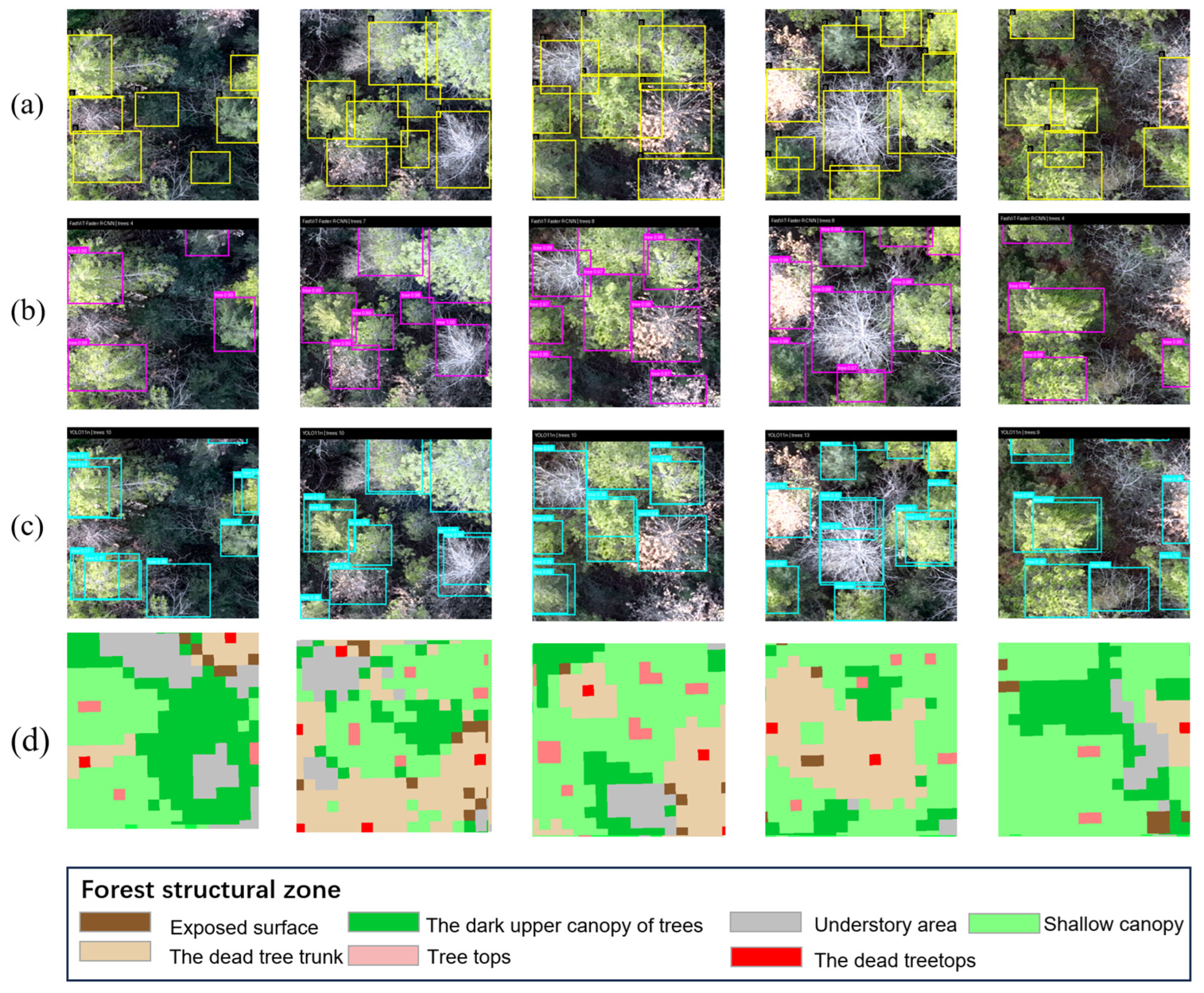
The practical distinction among workflows lies in their output nature: RGB detectors localize objects as isolated instances, whereas the FSZ workflow provides a continuous, wall-to-wall structural representation (Figure 11). In Domain A, this study highlights the unique diagnostic capability of the FSZ workflow by embedding discrete tree enumeration within a continuous structural context, thereby maximizing the utility of multidimensional UAV observations. Table 7 provides a contextual comparison with representative image-based studies; owing to differences in study settings and evaluation protocols, it is not intended as a strict cross-study ranking. While broader applicability requires further validation, the integrative framework offers a solid methodological foundation for multisource remote sensing in forest structure monitoring.

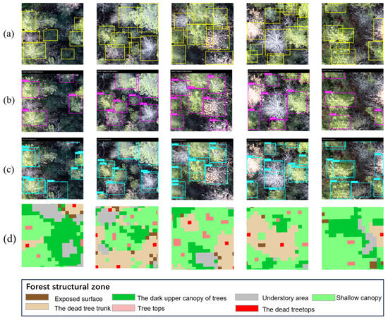
Figure 11. Qualitative comparison of five representative 416 × 416-pixel images from the independent standardized evaluation: (a) annotations, (b) FastViT-T8-FPN Faster R-CNN, (c) YOLO11n and (d) the refined FSZ map. Base classes are 1–6; secondary classification adds class 7 (dead treetops), which is excluded from the six-zone confusion-matrix evaluation.

Table 7. Comparison of the FSZ workflow with representative image-based tree-counting and crown-structure studies.

Metric	FSZ Domain A	FSZ Domain B	YOLO11n	FastViT-T8-FPN Faster R-CNN	Han et al. (2022) [53]	Osco et al. (2020) [54]	Pacheco-Prado et al. (2025) [55]	Popp & Kalwij (2023) [56]
Study category	Present study FSZ workflow	Present study FSZ workflow	Present study RGB detector	Present study RGB detector	Tree counting (UAV RGB image)	Tree counting (UAV multispectral image)	RGB crown-point-cloud classification	Tree-layer semantic segmentation
Tree-count MAE	1.889	/	1.889	1.667	2.135	2.050	/	/
Tree-count RMSE	2.517	/	2.472	2.236	3.274	3.13	/	/
Tree crown structure OA	82.5%	85.6%	/	/	/	/	70.0%	88.0%
Tree crown structure macro-F1	70.9%	75.1%	/	/	/	/	65.0%	/

4.1.2. Pixel-Level Deficits vs. Aggregate Counts in the Independent Domain B Validation

In the structurally complex Domain A, the pixel-level tree-top F1 was low (21.7%), whereas the six-zone macro-F1 was 70.9%. Subsequent connected-component extraction and peak-based splitting partly compensated for this pixel-level deficit, yielding a TCRE of −14.29%. In contrast, Domain B demonstrated substantially improved structural identification, with an OA of 85.6%, Kappa of 0.778, macro-F1 of 75.1%, and tree-top F1 rising to 34.0%, indicating that the structured planted canopies and higher spectral contrast effectively reduced confusion between tree tops and shallow canopy.

This contrast reflects the two complementary evaluation levels of the FSZ workflow. Macro-F1 summarizes discrimination across all six structural zones, whereas tree-top F1 isolates the most challenging apex-to-canopy transition. In the FSZ workflow, tree-top extraction is not based on a one-to-one conversion of individual classified pixels; spatially coherent residual tree-top signals are grouped into connected components, and merged candidate regions are resolved through peak-based splitting. This spatial aggregation converts the continuous FSZ map into discrete tree-top candidates and can recover tree tops despite local apex-to-canopy misclassification while retaining the surrounding structural context.

At the object level, however, Domain B achieved an F1 of 56.47% and a TCRE of −19.15%, reflecting a larger absolute underestimation than Domain A (−14.29%). This discrepancy is not attributed to a failure of the FSZ framework, but rather, to the more fragmented plot boundaries, artificial surfaces (such as roads and buildings), and dispersed crown spacing in urban-fringe environments, which pose more demanding spatial post-processing challenges requiring finer local parameter calibration. Overall, the superior structural classification in Domain B supports the potential of the FSZ workflow as a promising framework for urban-fringe monitoring. Alongside further optimization of local spatial parameters, refinement of tree-top annotation criteria, particularly at ambiguous apex-to-canopy transitions, offers a practical route to improving tree-top classification accuracy in future applications.

4.2. Applicability and Transferability Across Forest and Urban-Fringe Scenarios

The present results demonstrate consistent performance across two parallel scenarios: the dense, heterogeneous forest (Domain A) and the urban-fringe planted landscape (Domain B), which contains both dense and sparse trees. Both scenarios yielded promising results, indicating the workflow’s adaptability to various canopy structures. The workflow depends on consistent co-registration and on the spectral and structural characteristics of the multispectral, relative thermal-infrared, and CHM layers, and both RGB detectors and the FSZ workflow are sensitive to environmental variations. Domain A used its own training and holdout partitions. In Domain B, the Random Forest classification settings were retained, whereas only the tree-top extraction parameters were calibrated on a separate training partition before assessment on the final holdout subset. Since urban green spaces are often spatially fragmented, locally calibrated models are recommended. Unlike RGB detectors that treat trees as isolated instances, the FSZ workflow produces tree-count information alongside a continuous structural representation, offering a distinctive but complementary data product.

Given the site-based, exploratory nature of this study, the present results provide an initial foundation for broader deployment. Transferability to other forest types, acquisition dates, or UAV systems would require explicit adaptation and testing. Before application at a new site, input data and model settings should be verified [57]; likewise, annotation criteria, thresholds, and duplicate-removal rules for object detectors require specific examination [58]. Future applications should, therefore, prioritize targeted calibration of the FSZ classifier and spatial post-processing parameters to match the specific conditions of the new site.

4.3. Ecological Significance and Future Applications

4.3.1. Ecological and Management Implications of the FSZ Classes

The FSZ framework divides canopy surfaces into classes with distinct ecological and management interpretations. Tree tops and shallow canopy represent sunlit upper-canopy surfaces, supporting assessments of forest vitality and productivity when combined with field measurements [59]. The ‘dark upper canopy’ class captures three-dimensional rugosity and internal shading; a high proportion of shaded canopy indicates complex vertical structure, a recognized driver of microclimate buffering that regulates internal temperature and moisture levels [60]. Mapping these shaded regions offers spatially explicit data for assessing thermal regulation services in natural forests and urban green infrastructure.

The FSZ framework achieves two complementary objectives: it provides wall-to-wall continuous characterization of canopy-surface organization (e.g., illumination-driven zonation, height-derived layering, and canopy gaps), and it extracts discrete tree-top locations for abundance estimation. While individual-crown geometric metrics—such as diameter, area, or shape—are not directly validated in the present study, the framework’s design, which links pixel-level FSZ classification with connected-component extraction and peak-based splitting, inherently preserves the spatial footprint of each detected tree top. This structural foundation offers promising potential for future recovery of simplified crown-level attributes, particularly when combined with finer FSZ classification schemes, higher-resolution inputs, or optimized post-processing parameters. Such extensions, however, require dedicated field-validation data and are, therefore, identified as a key direction for subsequent investigation.

Dead tree trunks indicate standing deadwood relevant to habitat availability, pest monitoring, and fuel-load assessment, while understory and exposed surfaces identify canopy openings affecting understory light, regeneration, and erosion risk. These classes are spatial proxies rather than direct measurements of ecosystem functions, requiring field observations, calibrated environmental measurements, and independent validation for proper ecological interpretation [61,62].

4.3.2. Prospects for Urban Green-Infrastructure Monitoring

The primary experiment was conducted in a dense non-urban forest (Domain A), with an additional site-specific holdout evaluation in an urban-fringe planted landscape (Domain B). The workflow offers a repeatable and spatially explicit inventory of tree tops, making it relevant to urban green-infrastructure monitoring. Urban heat mitigation depends on tree presence, canopy structure, impervious surfaces, and local climate [63,64]. Geolocated tree-top counts provide basic metrics for monitoring density, survival, and canopy gaps, allowing repeated UAV surveys to map cooling assets, track canopy loss, and guide future planting. Broader urban application requires further adaptation and validation beyond the current site-specific holdout. Urban FSZ classes may need to distinguish tree crowns from roofs, roads, paved surfaces, building shadows, and mixed built–vegetated backgrounds [65]. Combining tree-top locations with crown size, calibrated temperature, impervious-cover data, and vulnerability indicators supports assessments of heat exposure, planting priorities, and equitable distribution of green-infrastructure benefits. Future applications should, therefore, integrate these complementary metrics across broader domains, such as carbon stock estimation, biodiversity assessment, forest health monitoring, sustainable urban planning, etc.

5. Conclusions

This study developed a multilayer FSZ workflow that integrates visible tree-top quantification with wall-to-wall characterization of forest structural conditions from co-registered UAV imagery. By combining multispectral, relative thermal-infrared, and canopy-height information, the workflow generates a six-zone FSZ map and derives tree-top estimates through spatial postprocessing. The FSZ workflow provides a complementary spatial data product that links tree-count information to the surrounding canopy structure. Its principal contribution is, therefore, the joint representation of discrete tree-top abundance and continuous forest structural patterns within a single framework.

The FSZ workflow was evaluated across two distinct scenarios. In the dense, heterogeneous forest of Domain A, it showed aggregate tree-count agreement, effectively supporting structural classification and tree-top extraction in a closed-canopy landscape. In the independent urban-fringe Domain B, the workflow also showed promising adaptability, effectively supporting structural classification and tree-top extraction in the more complex planted landscape.

Component extraction and peak splitting can reduce the influence of local pixel-level errors on aggregate counts but do not establish accurate identification of every individual tree. Given the site-based, exploratory nature of this study, the present results provide an initial foundation for broader deployment. Future applications should, therefore, prioritize targeted calibration of the FSZ classifier and spatial post-processing parameters to match local conditions, while this integrative framework offers a practical basis for extending multisource UAV monitoring across varying forest types and urban environments.

References

- Li, S.; Brandt, M.; Fensholt, R.; Kariryaa, A.; Igel, C.; Gieseke, F.; Nord-Larsen, T.; Oehmcke, S.; Carlsen, A.H.; Junttila, S.; et al. Deep Learning Enables Image-Based Tree Counting, Crown Segmentation, and Height Prediction at National Scale. PNAS Nexus 2023, 2, pgad076. [Google Scholar] [CrossRef] [Scilit] [PubMed]
- Zhao, H.; Morgenroth, J.; Pearse, G.; Schindler, J. A Systematic Review of Individual Tree Crown Detection and Delineation with Convolutional Neural Networks (CNN). Curr. For. Rep. 2023, 9, 149–170. [Google Scholar] [CrossRef] [Scilit]
- Liang, X.; Wang, Y.; Pan, J.; Heiskanen, J.; Wang, N.; Wu, S.; Vuorinne, I.; Tian, J.; Troles, J.; Cloutier, M.; et al. Empowering Tree-Scale Monitoring over Large Areas: Individual Tree Delineation from High-Resolution Imagery. ISPRS J. Photogramm. Remote Sens. 2026, 232, 974–999. [Google Scholar] [CrossRef] [Scilit]
- Chen, J.; Liang, X.; Liu, Z.; Gong, W.; Chen, Y.; Hyyppä, J.; Kukko, A.; Wang, Y. Tree Species Recognition from Close-Range Sensing: A Review. Remote Sens. Environ. 2024, 313, 114337. [Google Scholar] [CrossRef] [Scilit]
- Ventura, J.; Pawlak, C.; Honsberger, M.; Gonsalves, C.; Rice, J.; Love, N.L.R.; Han, S.; Nguyen, V.; Sugano, K.; Doremus, J.; et al. Individual Tree Detection in Large-Scale Urban Environments Using High-Resolution Multispectral Imagery. Int. J. Appl. Earth Obs. Geoinf. 2024, 130, 103848. [Google Scholar] [CrossRef] [Scilit]
- Fan, W.; Knoke, T.; Troles, J.; Tian, J. Automatic Tree-Level Based Forest Inventories Retrieval via Ultra-High Resolution UAV Images and Deep Learning. ISPRS J. Photogramm. Remote Sens. 2026, 234, 261–274. [Google Scholar] [CrossRef] [Scilit]
- Brandt, M.; Tucker, C.J.; Kariryaa, A.; Rasmussen, K.; Abel, C.; Small, J.; Chave, J.; Rasmussen, L.V.; Hiernaux, P.; Diouf, A.A.; et al. An Unexpectedly Large Count of Trees in the West African Sahara and Sahel. Nature 2020, 587, 78–82. [Google Scholar] [CrossRef] [Scilit] [PubMed]
- Tong, F.; Zhang, Y. Individual Tree Crown Delineation in High Resolution Aerial RGB Imagery Using StarDist-Based Model. Remote Sens. Environ. 2025, 319, 114618. [Google Scholar] [CrossRef] [Scilit]
- Zhang, C.; Song, C.; Zaforemska, A.; Zhang, J.; Gaulton, R.; Dai, W.; Xiao, W. Individual Tree Segmentation from UAS Lidar Data Based on Hierarchical Filtering and Clustering. Int. J. Digit. Earth 2024, 17, 2356124. [Google Scholar] [CrossRef] [Scilit]
- Deng, S.; Xu, Q.; Yue, Y.; Jing, S.; Wang, Y. Individual Tree Detection and Segmentation from Unmanned Aerial Vehicle-LiDAR Data Based on a Trunk Point Distribution Indicator. Comput. Electron. Agric. 2024, 218, 108717. [Google Scholar] [CrossRef] [Scilit]
- Dersch, S.; Schöttl, A.; Krzystek, P.; Heurich, M. Semi-Supervised Multi-Class Tree Crown Delineation Using Aerial Multispectral Imagery and Lidar Data. ISPRS J. Photogramm. Remote Sens. 2024, 216, 154–167. [Google Scholar] [CrossRef] [Scilit]
- Wielgosz, M.; Puliti, S.; Xiang, B.; Schindler, K.; Astrup, R. SegmentAnyTree: A Sensor and Platform Agnostic Deep Learning Model for Tree Segmentation Using Laser Scanning Data. Remote Sens. Environ. 2024, 313, 114367. [Google Scholar] [CrossRef] [Scilit]
- Park, G.; Song, B.; Park, K. Mapping Individual Tree Crowns to Extract Morphological Attributes in Urban Areas Using Unmanned Aerial Vehicle-Based LiDAR and RGB Data. Ecol. Inform. 2025, 88, 103165. [Google Scholar] [CrossRef] [Scilit]
- Dong, W.; Yuan, H.; Lin, W.; Liu, Z.; Xiang, J.; Wei, Z.; Li, L.; Li, Q.; Dai, Y. A Global Urban Tree Leaf Area Index Dataset for Urban Climate Modeling. Sci. Data 2025, 12, 426. [Google Scholar] [CrossRef] [Scilit] [PubMed]
- Vatandaslar, C.; Lee, T.; Bettinger, P.; Ucar, Z.; Stober, J.; Peduzzi, A. Mapping Percent Canopy Cover Using Individual Tree- and Area-Based Procedures That Are Based on Airborne LiDAR Data: Case Study from an Oak-Hickory-Pine Forest in the USA. Ecol. Indic. 2024, 167, 112710. [Google Scholar] [CrossRef] [Scilit]
- Velasquez-Camacho, L.; Cardil, A.; Mohan, M.; Etxegarai, M.; Anzaldi, G.; de-Miguel, S. Remotely Sensed Tree Characterization in Urban Areas: A Review. Remote Sens. 2021, 13, 4889. [Google Scholar] [CrossRef] [Scilit]
- Lin, J.; Ma, Q.; Ju, Y.; Zhang, H.; Wang, Q.; Huang, B. Relationships between Urbanization, Tree Morphology, and Carbon Density: An Integration of Remote Sensing, Allometric Models, and Field Survey. Urban For. Urban Green. 2022, 76, 127725. [Google Scholar] [CrossRef] [Scilit]
- Li, B.; Pang, Y.; Kükenbrink, D.; Wang, L.; Kong, D.; Marty, M. ITS-Net: A Platform and Sensor Agnostic 3D Deep Learning Model for Individual Tree Segmentation Using Aerial LiDAR Data. ISPRS J. Photogramm. Remote Sens. 2026, 231, 719–744. [Google Scholar] [CrossRef] [Scilit]
- Wang, Q.; Zhao, Y.; Che, Y.; Shen, H.; Qiu, Y.; Wang, Y. A Semi-Supervised Framework for UAV-Based Individual Tree Crown Segmentation in Structurally Heterogeneous Planted Forests. Int. J. Appl. Earth Obs. Geoinf. 2026, 146, 105078. [Google Scholar] [CrossRef] [Scilit]
- Guo, Q.; Li, K.; Qiao, X.; Jiang, J.; Zhao, Y. An Adaptive Method for Individual Tree Segmentation Synthesizing Canopy Cover and Competitive Mechanism Using UAV Data. Ecol. Inform. 2025, 91, 103360. [Google Scholar] [CrossRef] [Scilit]
- Jarahizadeh, S.; Salehi, B. Tree-Net: A Novel Deep Learning Tree Detection Architecture Using UAV LiDAR Data. Remote Sens. Environ. 2026, 332, 115088. [Google Scholar] [CrossRef] [Scilit]
- Zeng, J.; Shen, X.; Zhou, K.; Cao, L. FO-Net: An Advanced Deep Learning Network for Individual Tree Identification Using UAV High-Resolution Images. ISPRS J. Photogramm. Remote Sens. 2025, 220, 323–338. [Google Scholar] [CrossRef] [Scilit]
- Shi, J.; Li, H.; Jing, L.; Xiao, Z.; Zhou, H.; Zhang, Z.; Xu, S. ITC-YOLO: An Improved YOLOv8 Model for Individual Tree Crown Segmentation in Complex Forest Environments. Ecol. Indic. 2025, 180, 114355. [Google Scholar] [CrossRef] [Scilit]
- Jarahizadeh, S.; Salehi, B. Advancing Tree Detection in Forest Environments: A Deep Learning Object Detector Approach with UAV LiDAR Data. Urban For. Urban Green. 2025, 105, 128695. [Google Scholar] [CrossRef] [Scilit]
- Huo, Z.; Fang, L.; Chu, Y.; Dang, S.; Yang, J.; Li, L.; Li, X.; Ren, S.; Chen, J.; Peng, Y.; et al. Precise Urban Tree Species Identification and Biomass Estimation Using UAV–Handheld LiDAR Synergy and YOLOv11 Deep Learning. Int. J. Appl. Earth Obs. Geoinf. 2026, 146, 105049. [Google Scholar] [CrossRef] [Scilit]
- Zhou, H.; Zhang, X.; Zhang, C.; Ma, Q. Vision Transformer with Contrastive Learning for Hyperspectral Image Classification. IEEE Geosci. Remote Sens. Lett. 2023, 20, 5503905. [Google Scholar] [CrossRef] [Scilit]
- Han, K.; Wang, Y.; Chen, H.; Chen, X.; Guo, J.; Liu, Z.; Tang, Y.; Xiao, A.; Xu, C.; Xu, Y.; et al. A Survey on Vision Transformer. IEEE Trans. Pattern Anal. Mach. Intell. 2023, 45, 87–110. [Google Scholar] [CrossRef] [Scilit] [PubMed]
- Fu, H.; Zhao, H.; Jiang, J.; Zhang, Y.; Liu, G.; Xiao, W.; Du, S.; Guo, W.; Liu, X. Automatic Detection Tree Crown and Height Using Mask R-CNN Based on Unmanned Aerial Vehicles Images for Biomass Mapping. For. Ecol. Manag. 2024, 555, 121712. [Google Scholar] [CrossRef] [Scilit]
- Ibsen, P.C.; Crawford, B.R.; Corro, L.M.; Bagstad, K.J.; McNellis, B.E.; Jenerette, G.D.; Diffendorfer, J.E. Urban Tree Cover Provides Consistent Mitigation of Extreme Heat in Arid but Not Humid Cities. Sustain. Cities Soc. 2024, 113, 105677. [Google Scholar] [CrossRef] [Scilit]
- Li, H.; Zhao, Y.; Wang, C.; Ürge-Vorsatz, D.; Carmeliet, J.; Bardhan, R. Cooling Efficacy of Trees across Cities Is Determined by Background Climate, Urban Morphology, and Tree Trait. Commun. Earth Env. 2024, 5, 754. [Google Scholar] [CrossRef] [Scilit]
- Zaerpour, M.; Papalexiou, S.M.; Pietroniro, A. Increasing Tree Canopy Lowers Urban Air Temperature by up to 1.5 °C in Heat-Prone Areas. npj Urban Sustain. 2025, 5, 92. [Google Scholar] [CrossRef] [Scilit]
- McDonald, R.I.; Biswas, T.; Chakraborty, T.C.; Kroeger, T.; Cook-Patton, S.C.; Fargione, J.E. Current Inequality and Future Potential of US Urban Tree Cover for Reducing Heat-Related Health Impacts. npj Urban Sustain. 2024, 4, 18. [Google Scholar] [CrossRef] [Scilit]
- Osco, L.P.; Marcato Junior, J.; Marques Ramos, A.P.; De Castro Jorge, L.A.; Fatholahi, S.N.; De Andrade Silva, J.; Matsubara, E.T.; Pistori, H.; Gonçalves, W.N.; Li, J. A Review on Deep Learning in UAV Remote Sensing. Int. J. Appl. Earth Obs. Geoinf. 2021, 102, 102456. [Google Scholar] [CrossRef] [Scilit]
- Reilly, S.; Clark, M.L.; Loechler, L.; Spillane, J.; Kozanitas, M.; Krause, P.; Ackerly, D.; Bentley, L.P.; Menor, I.O. Unoccupied Aerial System (UAS) Structure-from-Motion Canopy Fuel Parameters: Multisite Area-Based Modelling across Forests in California, USA. Remote Sens. Environ. 2024, 312, 114310. [Google Scholar] [CrossRef] [Scilit]
- Tolan, J.; Yang, H.-I.; Nosarzewski, B.; Couairon, G.; Vo, H.V.; Brandt, J.; Spore, J.; Majumdar, S.; Haziza, D.; Vamaraju, J.; et al. Very High Resolution Canopy Height Maps from RGB Imagery Using Self-Supervised Vision Transformer and Convolutional Decoder Trained on Aerial Lidar. Remote Sens. Environ. 2024, 300, 113888. [Google Scholar] [CrossRef] [Scilit]
- Guimarães, N.; Sousa, J.J.; Couto, P.; Bento, A.; Pádua, L. Combining UAV-Based Multispectral and Thermal Infrared Data with Regression Modeling and SHAP Analysis for Predicting Stomatal Conductance in Almond Orchards. Remote Sens. 2024, 16, 2467. [Google Scholar] [CrossRef] [Scilit]
- Xie, Y.; Wang, Y.; Sun, Z.; Liang, R.; Ding, Z.; Wang, B.; Huang, S.; Sun, Y. Instance Segmentation and Stand-Scale Forest Mapping Based on UAV Images Derived RGB and CHM. Comput. Electron. Agric. 2024, 220, 108878. [Google Scholar] [CrossRef] [Scilit]
- Gui, S.; Song, S.; Qin, R.; Tang, Y. Remote Sensing Object Detection in the Deep Learning Era—A Review. Remote Sens. 2024, 16, 327. [Google Scholar] [CrossRef] [Scilit]
- Chehreh, B.; Moutinho, A.; Viegas, C. Latest Trends on Tree Classification and Segmentation Using UAV Data—A Review of Agroforestry Applications. Remote Sens. 2023, 15, 2263. [Google Scholar] [CrossRef] [Scilit]
- Kelly, J.; Kljun, N.; Olsson, P.-O.; Mihai, L.; Liljeblad, B.; Weslien, P.; Klemedtsson, L.; Eklundh, L. Challenges and Best Practices for Deriving Temperature Data from an Uncalibrated UAV Thermal Infrared Camera. Remote Sens. 2019, 11, 567. [Google Scholar] [CrossRef] [Scilit]
- Sagan, V.; Maimaitijiang, M.; Sidike, P.; Eblimit, K.; Peterson, K.; Hartling, S.; Esposito, F.; Khanal, K.; Newcomb, M.; Pauli, D.; et al. UAV-Based High Resolution Thermal Imaging for Vegetation Monitoring, and Plant Phenotyping Using ICI 8640 P, FLIR Vue pro R 640, and thermoMap Cameras. Remote Sens. 2019, 11, 330. [Google Scholar] [CrossRef] [Scilit]
- Ahmed, M.; El-Sheimy, N.; Leung, H.; Moussa, A. Enhancing Object Detection in Remote Sensing: A Hybrid YOLOv7 and Transformer Approach with Automatic Model Selection. Remote Sens. 2023, 16, 51. [Google Scholar] [CrossRef] [Scilit]
- Fan, K.; Li, Q.; Li, Q.; Zhong, G.; Chu, Y.; Le, Z.; Xu, Y.; Li, J. YOLO-Remote: An Object Detection Algorithm for Remote Sensing Targets. IEEE Access 2024, 12, 155654–155665. [Google Scholar] [CrossRef] [Scilit]
- Bera, S.; Shrivastava, V.K. Analysis of Various Optimizers on Deep Convolutional Neural Network Model in the Application of Hyperspectral Remote Sensing Image Classification. Int. J. Remote Sens. 2020, 41, 2664–2683. [Google Scholar] [CrossRef] [Scilit]
- Song, H.; Xie, J.; Wang, Y.; Fu, L.; Zhou, Y.; Zhou, X. Optimized Data Distribution Learning for Enhancing Vision Transformer-based Object Detection in Remote Sensing Images. Photogramm. Rec. 2025, 40, e70004. [Google Scholar] [CrossRef] [Scilit]
- Zhang, J.; Zhang, Y.; Shi, Z.; Zhang, Y.; Gao, R. Unmanned Aerial Vehicle Object Detection Based on Information-Preserving and Fine-Grained Feature Aggregation. Remote Sens. 2024, 16, 2590. [Google Scholar] [CrossRef] [Scilit]
- Anasosalu Vasu, P.K.; Gabriel, J.; Zhu, J.; Tuzel, O.; Ranjan, A. FastViT: A Fast Hybrid Vision Transformer Using Structural Reparameterization. In Proceedings of the 2023 IEEE/CVF International Conference on Computer Vision (ICCV); IEEE: Paris, France, 2023; pp. 5762–5772. [Google Scholar]
- Ren, S.; He, K.; Girshick, R.; Sun, J. Faster R-CNN: Towards Real-Time Object Detection with Region Proposal Networks. IEEE Trans. Pattern Anal. Mach. Intell. 2017, 39, 1137–1149. [Google Scholar] [CrossRef] [Scilit] [PubMed]
- Li, K.; Wang, D.; Wang, X.; Liu, G.; Wu, Z.; Wang, Q. Mixing Self-Attention and Convolution: A Unified Framework for Multisource Remote Sensing Data Classification. IEEE Trans. Geosci. Remote Sens. 2023, 61, 5523216. [Google Scholar] [CrossRef] [Scilit]
- Yang, B.; Wang, X.; Xing, Y.; Cheng, C.; Jiang, W.; Feng, Q. Modality Fusion Vision Transformer for Hyperspectral and LiDAR Data Collaborative Classification. IEEE J. Sel. Top. Appl. Earth Obs. Remote Sens. 2024, 17, 17052–17065. [Google Scholar] [CrossRef] [Scilit]
- Hartling, S.; Sagan, V.; Maimaitijiang, M. Urban Tree Species Classification Using UAV-Based Multi-Sensor Data Fusion and Machine Learning. GISci. Remote Sens. 2021, 58, 1250–1275. [Google Scholar] [CrossRef] [Scilit]
- Mohammadpour, P.; Viegas, C. Applications of Multi-source and Multi-sensor Data Fusion of Remote Sensing for Forest Species Mapping. In Advances in Remote Sensing for Forest Monitoring; Pandey, P.C., Arellano, P., Eds.; Wiley: Hoboken, NJ, USA, 2022; pp. 255–287. ISBN 978-1-119-78812-6. [Google Scholar]
- Han, P.; Ma, C.; Chen, J.; Chen, L.; Bu, S.; Xu, S.; Zhao, Y.; Zhang, C.; Hagino, T. Fast Tree Detection and Counting on UAVs for Sequential Aerial Images with Generating Orthophoto Mosaicing. Remote Sens. 2022, 14, 4113. [Google Scholar] [CrossRef] [Scilit]
- Osco, L.P.; Arruda, M.D.S.D.; Marcato Junior, J.; Da Silva, N.B.; Ramos, A.P.M.; Moryia, É.A.S.; Imai, N.N.; Pereira, D.R.; Creste, J.E.; Matsubara, E.T.; et al. A Convolutional Neural Network Approach for Counting and Geolocating Citrus-Trees in UAV Multispectral Imagery. ISPRS J. Photogramm. Remote Sens. 2020, 160, 97–106. [Google Scholar] [CrossRef] [Scilit]
- Pacheco-Prado, D.; Bravo-López, E.; Martínez, E.; Ruiz, L.Á. Urban Tree Species Identification Based on Crown RGB Point Clouds Using Random Forest and PointNet. Remote Sens. 2025, 17, 1863. [Google Scholar] [CrossRef] [Scilit]
- Popp, M.R.; Kalwij, J.M. Consumer-Grade UAV Imagery Facilitates Semantic Segmentation of Species-Rich Savanna Tree Layers. Sci. Rep. 2023, 13, 13892. [Google Scholar] [CrossRef] [Scilit] [PubMed]
- Chadwick, A.J.; Coops, N.C.; Bater, C.W.; Martens, L.A.; White, B. Transferability of a Mask R–CNN Model for the Delineation and Classification of Two Species of Regenerating Tree Crowns to Untrained Sites. Sci. Remote Sens. 2024, 9, 100109. [Google Scholar] [CrossRef] [Scilit]
- Zhou, X.; Hu, J.; Yan, S.; Li, C. Cognitive Experiments on Labelling Uncertainty for LCZ Mapping across Heterogeneous Megacities in China: Introducing Multi-Source Geospatial Data and LCZ Subclasses. Urban Clim. 2025, 63, 102599. [Google Scholar] [CrossRef] [Scilit]
- Li, F.; Hao, D.; Zhu, Q.; Yuan, K.; Braghiere, R.K.; He, L.; Luo, X.; Wei, S.; Riley, W.J.; Zeng, Y.; et al. Vegetation Clumping Modulates Global Photosynthesis through Adjusting Canopy Light Environment. Glob. Change Biol. 2023, 29, 731–746. [Google Scholar] [CrossRef] [Scilit] [PubMed]
- Ehbrecht, M.; Seidel, D.; Annighöfer, P.; Kreft, H.; Köhler, M.; Zemp, D.C.; Puettmann, K.; Nilus, R.; Babweteera, F.; Willim, K.; et al. Global Patterns and Climatic Controls of Forest Structural Complexity. Nat. Commun. 2021, 12, 519. [Google Scholar] [CrossRef] [Scilit] [PubMed]
- Muscolo, A.; Bagnato, S.; Sidari, M.; Mercurio, R. A Review of the Roles of Forest Canopy Gaps. J. For. Res. 2014, 25, 725–736. [Google Scholar] [CrossRef] [Scilit]
- Hoffmann, J.; Muro, J.; Dubovyk, O. Predicting Species and Structural Diversity of Temperate Forests with Satellite Remote Sensing and Deep Learning. Remote Sens. 2022, 14, 1631. [Google Scholar] [CrossRef] [Scilit]
- Ma, W.; Yu, Z.; Yang, W.; Zhang, Y.; Hu, Y.; Hu, J.; Zhang, H.; Yang, G. Optimizing Vegetation and Building Configurations for Streetscape Heat Mitigation: A Multi-Scale Analysis under Extreme Heat. Build. Environ. 2025, 283, 113331. [Google Scholar] [CrossRef] [Scilit]
- Li, C.; Xu, K.; Yan, S.; Ji, Q.; Zhang, D.; Zhou, X. Assessment of the Estimation Methods of Tmrt in Semi-Outdoor Spaces in Humid Sub-Tropical Climates: An Empirical Study in Wuhan, China. Build. Environ. 2024, 262, 111758. [Google Scholar] [CrossRef] [Scilit]
- Yan, J.; Zhou, W.; Han, L.; Qian, Y. Mapping Vegetation Functional Types in Urban Areas with WorldView-2 Imagery: Integrating Object-Based Classification with Phenology. Urban For. Urban Green. 2018, 31, 230–240. [Google Scholar] [CrossRef] [Scilit]
Disclaimer/Publisher’s Note: The statements, opinions and data contained in all publications are solely those of the individual author(s) and contributor(s) and not of MDPI and/or the editor(s). MDPI and/or the editor(s) disclaim responsibility for any injury to people or property resulting from any ideas, methods, instructions or products referred to in the content. |
© 2026 by the authors. Licensee MDPI, Basel, Switzerland. This article is an open access article distributed under the terms and conditions of the Creative Commons Attribution (CC BY) license.