Spatiotemporal Evolution of Land Use Patterns and Carbon Emission Effects in Hilly Regions

Abstract

Land use and land cover change represent major anthropogenic carbon emission sources, yet most existing studies on landscape patterns and carbon emissions predominantly focus on plain urban agglomerations, with limited empirical evidence from terrain-restricted hilly regions. Taking Xuancheng, a typical hilly city in the Yangtze River Delta, as the study area, this paper utilized seven time-series of Landsat remote-sensing datasets spanning 1990–2020. Integrating the land use dynamic degree, transfer matrix, landscape pattern indexes, calibrated carbon coefficients, Spearman correlation analysis and grey relational analysis, this study explored the associations between land use patterns and carbon emissions. Results show that built-up areas expanded 4.08-fold in the past three decades and emerged as the dominant carbon source, while forests maintained persistent carbon sequestration. The largest patch index of built-up area exhibited the strongest correlation with carbon emissions; cultivated land and forest displayed temporally synchronous fluctuations with emissions rather than exerting independent causal effects. Terrain constraints drive axial urban sprawl along transport corridors, elevating correlations of edge-related indexes and generating carbon response patterns distinct from those observed in plain cities. The two-step correlation analysis framework proved suitable for small-sample long-term datasets. These findings suggest that curbing contiguous built-up area expansion, optimizing urban morphology, and strengthening ecological connectivity should be prioritized in low-carbon spatial planning for hilly cities.

1. Introduction

Global climate change has emerged as one of the most critical challenges for sustainable development in the 21st century. Land use and land cover change (LUCC) constitutes the second largest source of carbon emissions globally, accounting for approximately one-third of total anthropogenic emissions. Urban areas, which occupy less than 3% of the global land area, contribute over 70% of worldwide carbon emissions. In 2020, China formally committed to achieving its carbon peak by 2030 and carbon neutrality by 2060. Territorial spatial planning provides a critical pathway toward these goals by optimizing land use structure and spatial layout. Nevertheless, most current low-carbon planning practices remain oriented towards energy restructuring and industrial upgrading, and insufficient attention has been paid to the carbon mitigation potential of land use morphological features. This research gap is particularly prominent in hilly cities, where topographic constraints promote land use patterns that differ substantially from those of plain regions.

Research on land use carbon emissions has established a relatively mature theoretical consensus: built-up areas function as the primary carbon source, whereas forest and grassland serve as major carbon sinks [1,2,3]; conversions across different land use categories directly reshape regional carbon budgets [4,5,6]. Empirical evidence from provincial and prefecture scales consistently demonstrates that emissions originating from built-up areas far outweigh emissions associated with alternative land use types [4,7,8,9]. Existing research largely emphasizes land use composition while overlooking spatial configuration effects: given identical total built-up area, compact versus scattered spatial layouts yield markedly different carbon emission magnitudes.

Advances in landscape ecology have shifted research focus from aggregate carbon output toward land use spatial forms [10]. When applied to carbon-related investigation, this analytical framework illustrates how urban morphology modulates carbon levels via transportation systems, energy consumption, and urban heat-island effects [11,12]. Cross-city comparisons confirm that compact, regular built layouts correspond to improved carbon emission performance, whereas fragmented configurations yield higher emission outputs; this principle also holds for cropland, green spaces, and mixed land types [13,14,15]. Municipal- and county-scale empirical studies further validate the idea that spatial configuration independently shapes local carbon outcomes [16,17,18,19]. Such coupling relationships are nonlinear and exhibit substantial spatial heterogeneity across river basins and urban agglomerations [20,21,22,23]. Prior work has identified total built-up area as a core determinant governing spatial differences in carbon emissions [24,25]. County-scale investigations additionally confirm that metrics including the largest patch index and landscape shape index can modulate local carbon emissions [26,27,28]. Grid-based analyses further document spatial mismatches between land use carbon outputs and landscape ecological risks [29]. Studies covering 20 urban agglomerations identify built-up areas and forests as the predominant carbon sources and sinks, respectively, while spatial configuration exerts carbon modulating effects distinct from simple land area composition [30,31,32]. Multiple scenario-simulation exercises verify that low-carbon development pathways can mitigate landscape fragmentation and reduce loss in ecosystem service provision [23,33,34,35].

Nearly all empirical evidence supporting the above-mentioned mechanisms originates from plain cities and large urban agglomerations [36,37]. It remains unclear whether these established rules apply to hilly urban settings constrained by mountain valley topography. Mountain barriers prevent complete radial sprawl and confine construction activities to linear strips aligned with transportation corridors. Extensive forest cover sustains stable regional carbon sinks, while scattered intermountain basins fragment built-up areas into disconnected patches. Whereas plain cities expand outward through continuous concentric rings across flat terrain, hilly cities can only develop axially along valley corridors. No prior studies have examined whether such morphological disparities alter correlation strengths between landscape pattern indexes and carbon emissions. Current mountainous zone-focused studies mostly compute carbon stock inventories or evaluate regional carbon balance [38,39,40], lacking long-term analyses exploring how landscape evolution modulates carbon emission performance in hilly urban areas.

Xuancheng City, situated in southeastern Anhui Province, China, is a typical hilly city within the Yangtze River Delta (YRD); its urban expansion trajectory fully embodies the terrain-driven developmental characteristics outlined above. Taking Xuancheng City as the research area, this study tested whether conclusions derived from plain cities remain generalizable and formulates three core research questions: How do land use quantities and landscape pattern indexes evolve under valley terrain constraints from 1990 to 2020? Compared with the concentric sprawl mode typical of plain cities, does axial expansion within hilly settings modify correlation magnitudes or correlation directions linking landscape indexes and carbon emissions? What targeted low-carbon territorial planning recommendations can be derived for analogous hilly cities based on this case study?

To address the above research questions, this study employed seven phases of Landsat remote sensing datasets spanning 1990–2020. Combining GIS spatial analysis, landscape pattern index computation, carbon emission coefficient accounting, and correlation analysis, this study systematically analyzed the spatiotemporal evolution characteristics of land use patterns and corresponding carbon emission effects in Xuancheng City.

2. Materials and Methods

2.1. Study Area

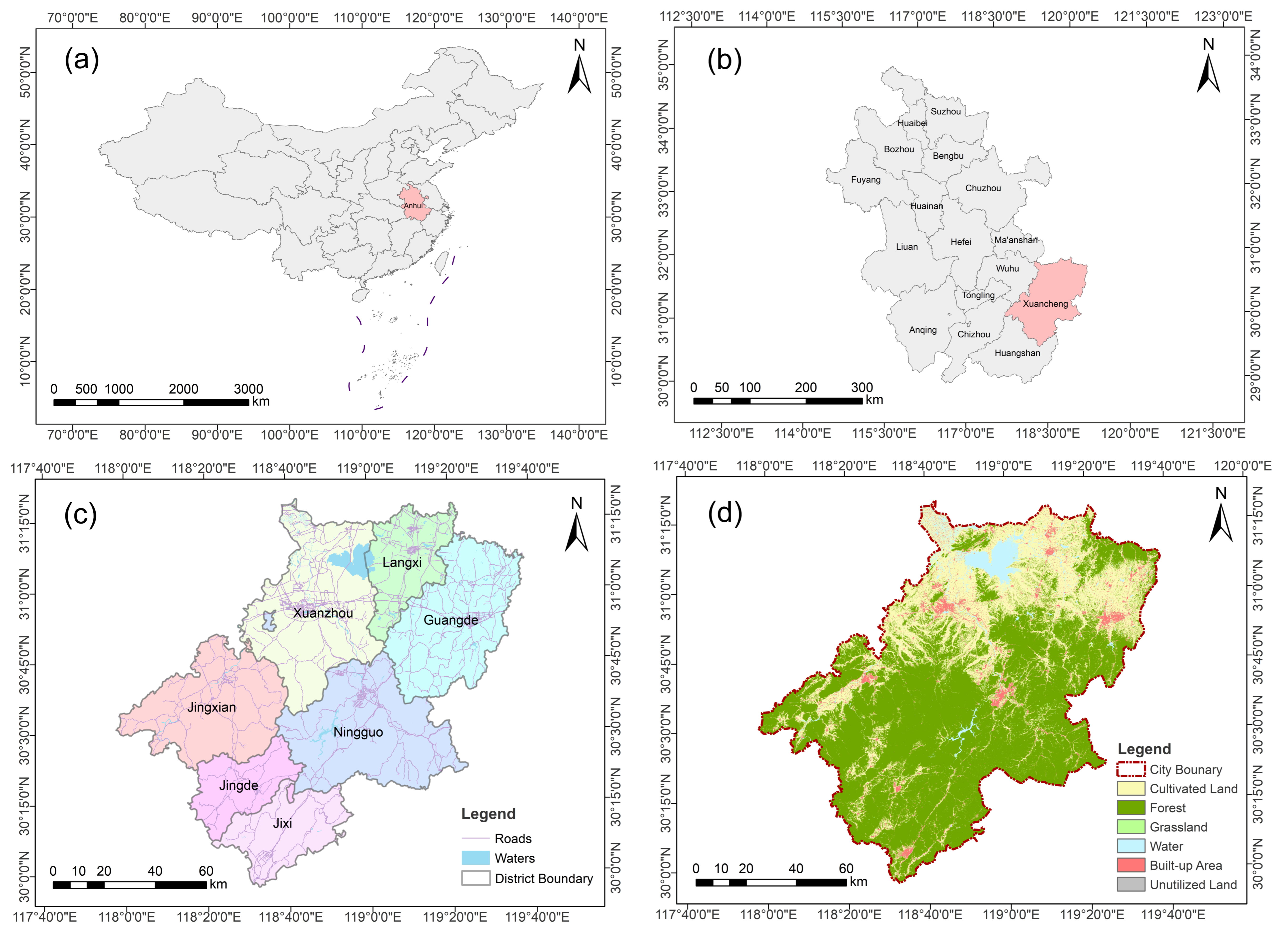
Xuancheng City (29°57′–31°19′ N, 117°58′–119°40′ E) functions as a gateway city linking southern Anhui Province with the YRD. It covers 12,312.58 km² and administers seven county-level administrative units, including Xuanzhou District, Langxi County, Guangde City, Ningguo City, Jing County, Jixi County, and Jingde County. The municipal government is seated within Xuanzhou District (Figure 1). As a key recipient zone for industrial transfer originating from the YRD, Xuancheng City underwent rapid industrialization and urbanization across the past three decades. By the end of 2020, its permanent resident population reached 2.5 million; urbanization equaled 57.00%; regional GDP totaled 160.75 billion CNY, and the industrial structure ratio of primary, secondary, and tertiary industries stood at 10.1:47.2:42.7.

Figure 1. Geographical location and land cover of Xuancheng City. (a) Location of Anhui Province in China; (b) location of Xuancheng City in Anhui Province; (c) administrative division of Xuancheng City; (d) land cover of Xuancheng City.

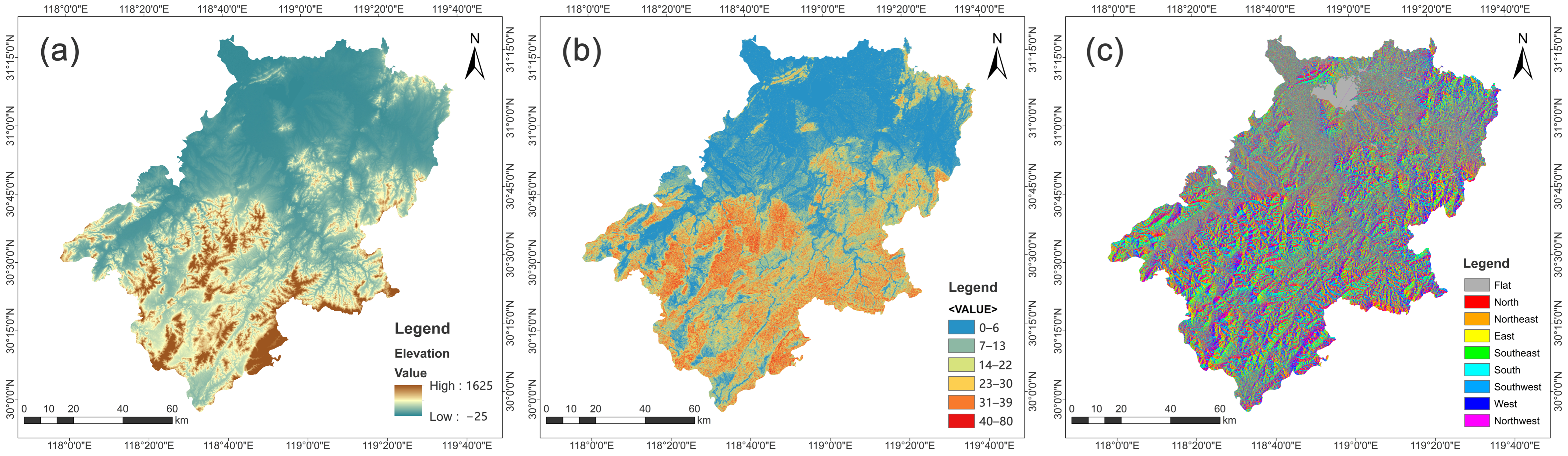
Its terrain descends stepwise from the southeast toward the northwest, featuring mid-elevation mountains across southern zones, rolling hills in central portions, and alluvial plains to the north. It forms a characteristic hilly-region landscape pattern described as “six parts mountain, one part water, two parts farmland, and one part roads and settlements”, with hilly and mountainous terrain occupying more than 70% of its total territory (Figure 2). Forest coverage reaches 59.46%, rendering it a critical ecological barrier and carbon sink base for the YRD. This combination of high-quality ecological endowment, rapid urban development pressures, and pronounced topographic constraints makes Xuancheng City an ideal case for investigating the linkages between land use evolution and carbon emissions within hilly city contexts.

Figure 2. Topographic analysis of Xuancheng City: (a) elevation; (b) slope; (c) aspect.

2.2. Data Sources

Datasets adopted for this study primarily comprise multi-temporal land use data, digital elevation model (DEM) data, administrative boundary datasets, major road network data, and socio-economic statistical records. Detailed specifications, sources, and analytical purposes for each dataset are summarized within Table 1. All spatial layers are re-projected to the WGS 1984 UTM Zone 50N coordinate system. Raster datasets possessing disparate native resolutions were resampled to a uniform 30 m pixel resolution and clipped against Xuancheng’s administrative boundary, guaranteeing consistent spatial extent, pixel dimension and projection across all spatial analysis workflows.

Table 1. Data sources and uses.

Data	Reference Year	Resolution	Sources	Data Uses
Land use data	1990, 1995, 2000, 2005, 2010, 2015, 2020	30 m × 30 m	GLC_FCS30D, Aerospace Information Research Institute, Chinese Academy of Sciences (https://data.casearth.cn)	Detect land use spatiotemporal shifts; compute landscape pattern indexes; quantify land use carbon emissions
Digital elevation model (DEM)	2000	30 m × 30 m	SRTM V3, Geospatial Data Cloud (http://www.gscloud.cn)	Derive elevation, slope and aspect to interpret topographic constraints on land use evolution
Administrative boundary data	2020	-	National Geomatics Center of China (https://www.ngcc.cn)	Generate study area mask for raster clipping and spatial boundary calibration
Trunk road network data	2020	-	National Geomatics Center of China (https://www.ngcc.cn)	Create multi-scale buffer zones (300 m, 500 m, 1 km, 2 km) to quantify built-up area sprawl along transportation corridors
Socio-economic statistical data	1990–2020	-	Xuancheng Statistical Yearbooks (1991–2021), Xuancheng Municipal Bureau of Statistics (https://tjj.xuancheng.gov.cn)	Calibrate localized carbon emission coefficients; supplement socioeconomic driving factor analysis

2.3. Methods

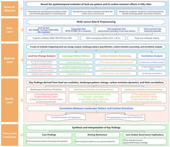
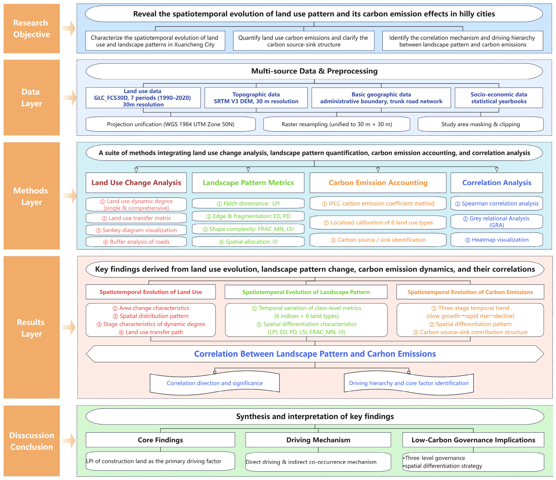
Figure 3 presents the complete sequential analytical workflow implemented within this study, encompassing land use change detection, traffic corridor spatial statistics, landscape morphological quantification, carbon budget accounting, and factor coupling analysis. Rationales justifying method selection and detailed implementation procedures for each analytical technique are elaborated within subsequent subsections.

Figure 3. Research framework of this study.

2.3.1. Land Use Dynamic Degree

To quantify the magnitude and rate of land use transformation, two metrics were adopted: single and comprehensive land use dynamic degrees. The single dynamic degree quantifies the magnitude and rate of area change for an individual land use category across a given time interval [41]. The calculation formula is as follows:

$$K={\displaystyle \frac{U_b-U_a}{U_a}}\times {\displaystyle \frac{1}{T}}\times 100\%$$

(1)

where K is single land use dynamic degree; U_a and U_b represent the area of a given land use type at the initial and final stage of the study period (km²), respectively; and T denotes the time interval (years). The interval between adjacent remote sensing images in this study is 5 years, thus T = 5. A positive K value indicates expansion, while a negative indicates contraction. A larger absolute K corresponds to a more intensive land use conversion activity.

The comprehensive dynamic degree quantifies aggregate transformation intensity across all land use categories [42], reflecting the total anthropogenic disturbance imposed upon the regional land use system. The calculation formula is as follows:

$$LC={\displaystyle \frac{{\sum }_{i=1}^n|∆{LU}_i|}{2\times {\sum }_{i=1}^n{LU}_i}}\times {\displaystyle \frac{1}{T}}\times 100\%$$

(2)

where LC is the comprehensive dynamic degree (%·a⁻¹), ΔLU_i represents area change of the i-th land use type (km²), and ∣ΔLU_i∣ is its absolute value, LU_i is the area of the i-th land use type at the initial stage (km²), and n is the total number of land use classes. In this study, land use is classified into six categories: cultivated land, forest, grassland, water, built-up area, and unutilized land, so n = 6, while T is the time interval (5 years). Higher LC values signify more active overall land use transitions.

2.3.2. Land Use Transfer Matrix

To identify conversion pathways between distinct land use categories, land use transfer matrices were constructed for six intervals: 1990–1995, 1995–2000, 2000–2005, 2005–2010, 2010–2015, and 2015–2020. This matrix quantifies the magnitude and directional patterns of cross-category land use conversions [43,44]. It should be noted that the transfer matrix only documents areal conversion relationships; spatial distribution attributes are further assessed via overlay analysis in ArcMap 10.5.

To intuitively visualize dominant conversion pathways and long-term evolutionary trajectories, Sankey diagrams were deployed to illustrate 1990–2020 land use transfer patterns derived from multi-period matrix outputs. Nodes denote distinct land use categories, and flow ribbons represent transferred land area [45].

2.3.3. Buffer Analysis of Transport Corridors

To validate the spatially directional urban expansion-aligned transport corridors, buffer-zone analysis was performed using trunk road network vector data. Multi-ring buffer zones (300 m, 500 m, 1 km, and 2 km) were generated surrounding all major roads features. The fraction of total built-up area falling inside each buffer zone was computed for each of the seven observational epochs [46]. The calculation of the formula is as follows:

$$P_d={\displaystyle \frac{A_{\_\mathrm{b}\mathrm{u}\mathrm{i}\mathrm{l}\mathrm{t}\_\mathrm{u}\mathrm{p}\_\mathrm{w}\mathrm{i}\mathrm{t}\mathrm{h}\mathrm{i}\mathrm{n}\_\mathrm{b}\mathrm{u}\mathrm{f}\mathrm{f}\mathrm{e}\mathrm{r}}}{A_{\_\mathrm{b}\mathrm{u}\mathrm{i}\mathrm{l}\mathrm{t}\_\mathrm{t}\mathrm{o}\mathrm{t}\mathrm{a}\mathrm{l}}}}\times 100\%$$

(3)

where d represents the buffer distance; A_{_built_up_within_buffer} is the built-up area inside the buffer of distance d; and A_{_built_up_total} is the total built-up area across Xuancheng City. Following standard urban expansion conventions [36], the 1 km buffer was selected as the primary analytical scale, with 300 m, 500 m, and 2 km buffers as supplementary reference scales.

2.3.4. Landscape Pattern Index

To characterize the spatial morphological attributes for each land use class, six class-level landscape pattern metrics were selected, covering patch dominance, fragmentation intensity, shape complexity, edge properties, and spatial interspersion [40]. All metrics were computed within Fragstats 4.2 software using the 8-neighborhood analysis rule applied to reclassified 30 m-resolution land use raster datasets [47]. Metric definitions and ecological interpretations are provided in Table 2.

Table 2. Definitions of landscape indexes selected.

Index	Abbreviation	Description and Selection Justification
Largest patch index	LPI	Percentage of total landscape area comprising the largest patch. Reflects the dominance of a single large contiguous patch
Edge density	ED	Total edge length per unit area, indicating landscape dissection
Mean fractal dimension index	FRAC_MN	Quantifies patch shape complexity, values near 1 indicate simple regular shapes, values near 2 indicate highly complex shapes
Landscape shape index	LSI	Measures overall landscape shape irregularity
Patch density	PD	Number of patches per unit area, directly indicating landscape fragmentation
Interspersion and juxtaposition index	IJI	Reflects the degree of intermixing among different land use types

2.3.5. Carbon Emission Coefficient Method

For estimating land use category-specific carbon emissions, this study implemented the IPCC-recommended carbon emission coefficient approach [48]. The accounting formula is as follows:

$$E={\displaystyle \sum _{i=1}^6}{S}_i\times T_i$$

(4)

where E is the total carbon emission (tC), S_i s refers to the area of the i-th land use type (m²), and T_i represents the per-unit-area carbon emission coefficient for the i-th land use class (g·m-²·a⁻¹). Positive values denote carbon sources, negative values represent carbon sinks.

To ensure the coefficients adequately reflect local Xuancheng conditions, localized corrections were implemented informed by regional industrial composition, vegetation traits, cropping regimes, and hydrological characteristics. For built-up areas, baseline coefficient was obtained from Tang et al., and subsequently adjusted using the following:

$$T_{\_built\_up \_local}=T_{\_built\_up\_base}\times \left(1+\alpha \times \Delta I_{\_secondary}\right)$$

(5)

where ΔI_{_secondary} is deviation in secondary industry GDP share relative to 1990 baseline year for Xuancheng and α is a regional adjustment coefficient (α = 0.028) calibrated against provincial-level energy-consumption statistics sourced from the Anhui Statistical Yearbook. Calibration rationales for each land use category, together with original baseline coefficients and corresponding citations, are summarized in Table 3 for transparency.

Table 3. Carbon emission coefficients of different land use types.

Land Use Type	Base Coefficient (g/(m2·a))	Local Coefficient (g/(m2·a))	Calibration Justification
Cultivated land	48.2 [4]	49.7	Rice–rapeseed rotation system; fertilizer application intensity from statistical yearbooks
Forest	−62.0 [49]	−58.1	Biomass weighting of regional major species (Chinese fir, masson pine, evergreen broad-leaved forest)
Grassland	−2.51 [1]	−2.1	Reference mean from similar studies in hilly regions
Water	−25.3 [50]	−25.3	Consistent with carbon cycle characteristics of Shuiyang River system and Nanyi Lake
Built-up area	3500 [1]	3607	Adjusted by secondary industry proportion (α = 0.028) using Formula (5)
Unutilized land	−0.5 [51]	−0.5	General standard value for regional-scale land use

2.3.6. Spearman Correlation Analysis

Spearman correlation analysis was applied to quantify statistical associations linking landscape pattern indexes and carbon emissions. This non-parametric technique assess monotonic correlation strength by computing rank concordance across paired variables. It does not impose normality or linearity assumptions, rendering it well suited for the seven-epoch small-sample time-series datasets in this study [6,52]. The calculation formula is as follows:

$$r_s=1-{\displaystyle \frac{6{\sum }_{i=1}^n{d}_i^2}{n(n^2-1)}}$$

(6)

where r_s is the Spearman correlation coefficient with a value range of [−1, 1]; d_i represents the rank difference of two variables in the i-th sample group; and n is the sample count. Positive r_s corresponds to positive correlation, negative values indicates negative correlation. The closer the absolute value is to 1, the stronger the monotonic correlation between variables. Exact p-values are reported alongside all correlation coefficients.

2.3.7. Grey Relational Analysis

Grey relational analysis (GRA) was implemented to rank relative influence magnitudes for landscape pattern indexes acting upon carbon emissions. While Spearman correlation identifies direction and statistical significance, it cannot quantify relative factor influence magnitudes; GRA addresses this limitation by evaluating similarity among temporal variation trajectories for landscape indexes and carbon emission time series. GRA imposes minimal constraints regarding sample-size distribution properties and is therefore compatible with these datasets [53,54]. The calculation steps are as follows:

•

Sequence construction: Time-series data of total regional carbon emissions from 1990 to 2020 are taken as the reference sequence X₀(k); the time-series data of various landscape pattern indexes are taken as the comparison sequences X_i(k), where k = 1, 2, …, 7 corresponds to the seven study periods (1990–2020).

•

Dimensionless processing: An initial value normalization method is deployed to eliminate the dimensional and magnitude differences of all sequences:

$$X_i^{\prime }(k)={\displaystyle \frac{X_i\left(k\right)}{X_i\left(1\right)}}$$

(7)

where $X_i^{\prime }\left(k\right)$ is the normalized value of index i at time-point k and X_i(1) is the initial value (1990) of comparison sequence i.

•

Difference sequence and extremum calculation: Calculate the absolute difference between comparison sequences and the reference sequence to construct the difference sequence, and determine the global maximum difference ∆_max and global minimum difference ∆_min:

$${{\Delta }_i=|X}_0^{\prime }\left(k\right)-X_i^{\prime }\left(k\right)|$$

(8)

•

Correlation coefficient calculation: The distinguishing coefficient ρ is introduced to weaken the interference of extreme values and the universal industry standard value ρ = 0.5 is adopted. The relational coefficient ξ_i(k) formula is as follows:

$${\xi }_i(k)={\displaystyle \frac{{∆}_{min}+\rho \times {∆}_{max}}{{∆}_i\left(k\right)+\rho \times {∆}_{max}}}$$

(9)

•

Grey correlation degree calculation: The average value of correlation coefficients at all time nodes is calculated to obtain the grey correlation degree r_i between each landscape index and carbon emissions:

$$r_i={\displaystyle \frac{1}{n}}{\sum }_{k=1}^n{\xi }_i\left(k\right)$$

(10)

Grey correlation degree range over (0, 1]. Values closer to 1 indicate higher temporal trend coherence and stronger correlative driving relationships between landscape indexes and carbon emissions. Based on rank-ordered relational-degree outputs, this study clarifies influence hierarchies and predominant landscape factors shaping carbon emission dynamics within hilly cities.

3. Results

3.1. Temporal and Spatial Evolution of Land Use

3.1.1. Characteristics of Area Change

Forest and cultivated land dominated Xuancheng’s land use structure across 1990–2020, collectively accounting for over 90% of total land area (Table 4). Built-up area exhibited the most dramatic growth, expanding from below 100 km² to over 500 km², representing approximately four-fold areal growth, with its proportional share rising from below 1% to over 4%. Cultivated land declined by more than 400 km², it was predominantly converted toward built-up land, with partial conversion back to forest via ecological restoration programs. Forest cover remained relatively stable above 62%, subject only to minor fluctuations. Grassland area expanded from 28.76 km² to 109.86 km², and water bodies increased from 379.43 km² to 454.17 km², reflecting ecological restoration and water conservancy construction activities. Unutilized land remained negligible areal magnitudes throughout the study period.

Table 4. Area and proportion of each land use type in Xuancheng City, 1990–2020.

Year Land Use Type	Cultivated Land		Forest		Grassland		Water		Built-Up Area		Unutilized Land
	Area (km2)	Proportion (%)	Area (km2)	Proportion (%)	Area (km2)	Proportion (%)	Area (km2)	Proportion (%)	Area (km2)	Proportion (%)	Area (km2)	Proportion (%)
1990	3980.90	32.33	7823.88	63.54	28.76	0.23	379.43	3.08	99.61	0.81	0.00	0.00
1995	3948.85	32.07	7855.92	63.80	17.46	0.14	374.36	3.04	115.97	0.94	0.00	0.00
2000	3585.67	29.12	8080.98	65.63	27.54	0.22	396.57	3.22	221.80	1.80	0.02	0.00
2005	3538.78	28.74	8021.14	65.15	58.75	0.48	396.46	3.22	297.39	2.42	0.05	0.00
2010	3537.96	28.73	7923.53	64.35	43.30	0.35	415.24	3.37	392.53	3.19	0.01	0.00
2015	3466.48	28.15	7789.25	63.26	75.07	0.61	451.80	3.67	529.77	4.30	0.20	0.00
2020	3570.77	29.00	7670.12	62.29	109.86	0.89	454.17	3.69	506.40	4.11	1.25	0.01

3.1.2. Characteristics of Spatial Distribution

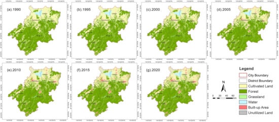
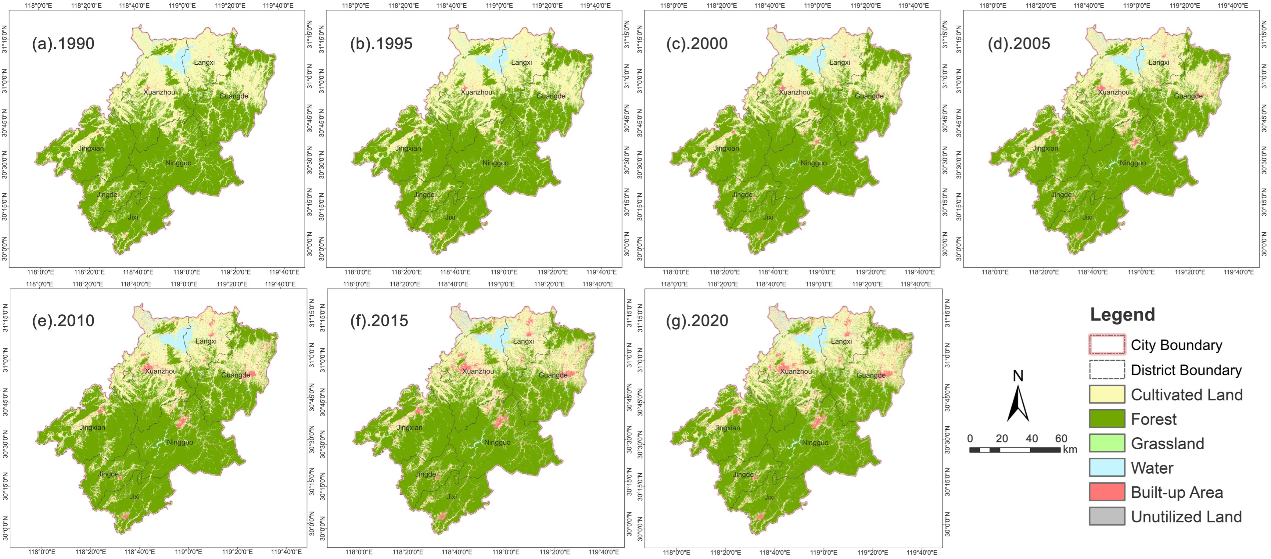
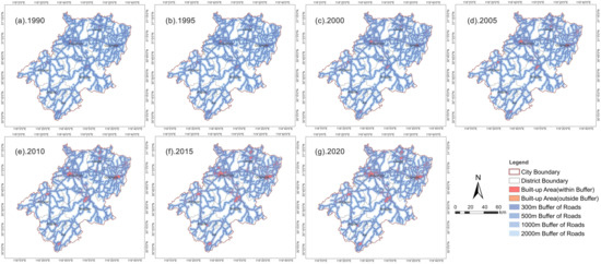
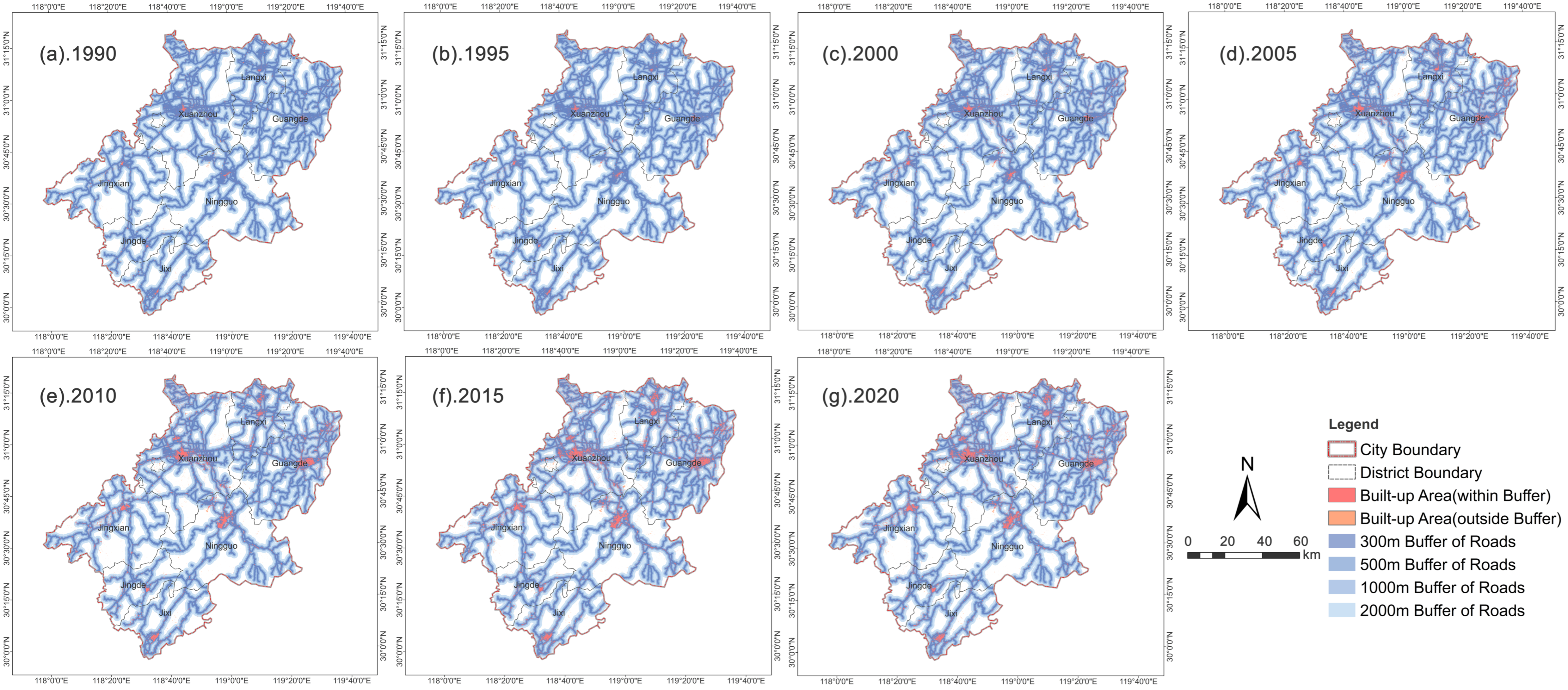
Xuancheng’s land use configuration exhibited a pronounced north–south spatial divide: cultivated land prevailed across northern alluvial plains, while extensive contiguous forest occupied southern mountainous terrain. Built-up areas were concentrated alongside transportation corridors (Figure 4). This corridor-anchored spatial pattern intensified over time, as built-up expansion radiated outward from central city and county seat locations following roads and waterways. Buffer-zone mapping (Figure 5) reveals built-up areas heavily concentrated within the 2 km road proximity zone, achieving the highest densities within the innermost 300 m buffer band. Multi-distance buffer quantitative outputs (Table 5) corroborate the pattern. The proportion of built-up areas situated within 1 km of major roads remained consistently high, climbing from 86.1% in 1990 to 89.0% in 2020, indicating persistent spatial proximity between new construction and transport infrastructure. The 300 m buffer share rose from 64.1% to 69.5%, demonstrating that newly added built-up land became progressively situated closer to major road networks. Across the study period, over 95% of built-up areas fell within 2 km of major transportation arteries. This persistent corridor-oriented distribution confirms that urban expansion in Xuancheng was strongly channeled along transport corridors, a defining feature of valley-constrained hilly city urban morphology. Southern forest zones remained spatially stable, whereas northern and central region landscapes experienced intensive urban-driven transformation.

Figure 4. Spatial distribution of land use in Xuancheng City, 1990–2020.

Figure 5. Buffer zones of main roads and built-up area distribution in Xuancheng City, 1990–2020.

Table 5. Built-up area within different buffer distances of main roads in Xuancheng City, 1990–2020.

Year	Built-Up Area (km2)	Falling Within 300 m		Falling Within 500 m		Falling Within 1 km		Falling Within 2 km
		Area (km2)	Proportion (%)	Area (km2)	Proportion (%)	Area (km2)	Proportion (%)	Area (km2)	Proportion (%)
1990	99.61	63.81	64.07	74.10	74.40	85.71	86.05	94.72	95.09
1995	115.97	75.09	64.74	86.84	74.88	99.97	86.20	110.25	95.06
2000	221.80	143.61	64.75	164.40	74.12	190.59	85.93	212.01	95.59
2005	297.39	199.82	67.19	226.99	76.33	259.97	87.42	285.18	95.89
2010	392.53	273.17	69.59	308.30	78.54	347.98	88.65	377.55	96.18
2015	529.77	363.77	68.67	412.51	77.86	469.28	88.58	509.45	96.16
2020	506.40	351.77	69.46	397.59	78.51	450.52	88.96	487.74	96.31

3.1.3. Land Use Dynamic Degree

Single dynamic degree outputs (Table 6) show an inverted-V trajectory for built-up area change: this peaked at an annual rate of 18.25% for 1995–2000, declined to 6.99% during 2010–2015, and turned negative for the first time over 2015–2020 under territorial spatial regulation policy interventions. Cultivated land dynamic degree values were predominantly negative; the sharpest contraction occurred for 1995–2000, and values reverted to positive for 2015–2020 due to arable land occupation compensation balance policies. Forest exhibited weakly positive growth exclusively over 1995–2000, driven by the Grain-for-Green ecological restoration initiative. Grassland yielded high dynamic degree values because of its small baseline area, although absolute areal modifications stayed limited. The comprehensive dynamic degree time series display a dual-peak profile: maxima appeared for 1995–2000 and for 2010–2015, corresponding respectively to the early-stage industrialization and the industrial transfer receipt phase originating from the YRD. Dynamic degree magnitudes decreased after 2015, signifying stabilized land use conversion and regulatory policy effects.

Table 6. The single and comprehensive dynamic degree of land use in Xuancheng City, 1990–2020.

Period	Cultivated Land (%·a−1)	Forest (%·a−1)	Grassland (%·a−1)	Water (%·a−1)	Built-Up Area (%·a−1)	Unutilized Land (%·a−1)	Comprehensive Dynamic Degree (%·a−1)
1990–1995	−0.16	0.08	−7.85	−0.27	3.29	0.00	0.08
1995–2000	−1.84	0.57	11.54	1.19	18.25	400.00	0.59
2000–2005	−0.26	−0.15	22.67	−0.01	6.82	35.24	0.17
2005–2010	0.00	−0.24	−5.26	0.95	6.40	−15.17	0.19
2010–2015	−0.40	−0.34	14.67	1.76	6.99	340.00	0.33
2015–2020	0.60	−0.31	9.27	0.10	−0.88	105.16	0.23

3.1.4. Land Use Transfer Matrix

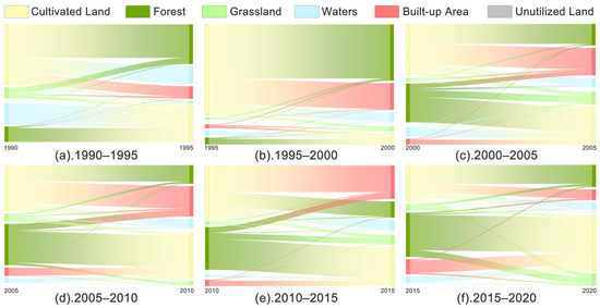
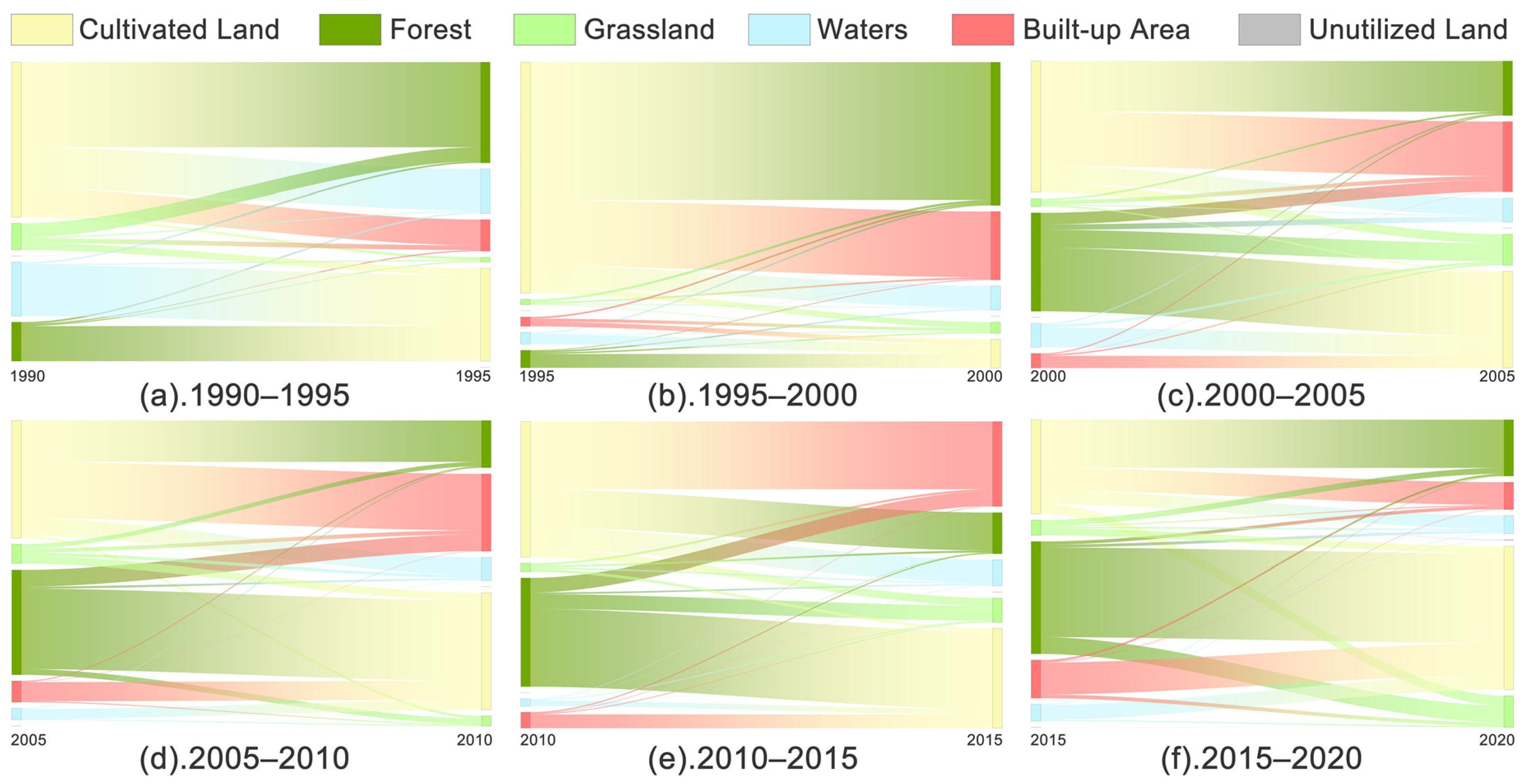
Sankey diagram visualizations (Figure 6) derived from land use transfer records (Table A1, Table A2, Table A3, Table A4, Table A5 and Table A6) demonstrate that 30-year land use conversions were dominated by cultivated land conversions toward forest and built-up area, with distinct stage-specific traits. During 1990–2000, the Grain-for-Green policy drove the cultivation of land to forest as the primary transformation pathway, accompanied by gradual built-up area expansion. For 2000–2015, rapid urbanization rendered built-up areas the dominant land use-inflow category; bidirectional conversion activity intensified between cultivated land and forest, amplifying trade-offs between agricultural production space and ecological space. Over 2015–2020, the cultivated transfers of land to built-up areas contracted substantially, while reciprocal conversions between cultivated land and forest became more prominent, producing net cultivated land area gains and effective containment of uncontrolled built-up area expansion.

Figure 6. Sankey diagram of land use transfer in Xuancheng City, 1990–2020 (for clarity, this omits intra-category transfer flows, as these lines would be visually indistinguishable due to the extremely small area of unutilized land.).

Four core characteristics emerge from the transfer matrix analysis. First, inflow sources exhibit strong concentration: over 90% of newly created built-up areas originated from cultivated land and forest conversion. Second, bidirectional conversion activity intensified over time, shifting from early-period one-way encroachment toward later-stage two-way circulation. Third, policy-driven orientations are prominent: conversion pathways for each time interval closely aligned with national-level policy priorities. Fourth, spatial patterns evolved from scattered patch distribution toward bead-style agglomeration aligned with transportation corridors.

3.2. Temporal and Spatial Evolution of Landscape Pattern

3.2.1. Changes of Landscape Pattern Indexes for Each Land Use Type

Cultivated land experienced diminishing patch dominance, intensifying fragmentation, growing morphological complexity, and rising spatial interspersion over the 30-year period (Table 7). LPI decreased from 26.77 to 21.47 (a nearly 20% reduction), indicating shrinkage of large contiguous core patches. PD increased by 46.5%. ED and LSI rose by 36.5% and 44.0%, respectively. IJI climbed from 49.13 to 64.11, reflecting heightened mosaic intermixing across cultivated land, forest, and built-up area patches.

Table 7. Landscape pattern indexes of cultivated land in Xuancheng City, 1990–2020.

Year Index	LPI	ED	FRAC_MN	PD	LSI	IJI
1990	26.77	45.46	1.04	3.21	222.84	49.13
1995	26.54	45.11	1.04	3.04	222.01	48.99
2000	22.16	47.44	1.04	3.15	244.93	54.73
2005	14.75	50.58	1.04	3.44	262.77	57.74
2010	21.90	54.11	1.04	3.76	281.16	56.82
2015	14.54	59.34	1.04	4.44	311.33	61.69
2020	21.47	62.06	1.04	4.70	320.84	64.11

Forests maintained broadly stable landscape configurations while undergoing slow-progressive degradation (Table 8). LPI consistently exceeded 50, documenting well-preserved large core ecological patches situated within southern mountain zones. PD increased by 61.05%, as forest patches fragmented across northern plain and hilly region locations. ED and LSI increased by 23.35% and 24.19%, respectively. IJI grew by 106.06%, representing expanding interspersion between forest and alternative land use classes.

Table 8. Landscape pattern index of forest in Xuancheng City, 1990–2020.

Year Index	LPI	ED	FRAC_MN	PD	LSI	IJI
1990	51.94	35.98	1.04	2.67	127.30	15.19
1995	51.94	35.04	1.04	2.53	123.78	13.13
2000	53.34	35.22	1.04	2.86	122.70	19.09
2005	53.23	37.80	1.04	3.43	132.03	24.87
2010	52.79	40.01	1.04	3.75	140.44	23.87
2015	51.79	42.37	1.04	3.96	149.90	29.42
2020	50.99	44.38	1.04	4.30	158.10	31.39

Built-up areas underwent the most substantial landscape configuration transformations (Table 9). LPI increased more than nine-fold, reflecting the rapid enlargement of contiguous urban core patches. PD rose by 60.7%, following an evolutionary trajectory characterized by scattered outward-patch expansion in early periods and progressive spatial consolidation in later years. ED and LSI increased by 199.26% and 33.06%, respectively. FRAC_MN and IJI both increased concurrently, corresponding to expanding urban–rural ecotone zones.

Table 9. Landscape pattern index of built-up areas in Xuancheng City, 1990–2020.

Year Index	LPI	ED	FRAC_MN	PD	LSI	IJI
1990	0.03	5.40	1.03	2.09	166.50	29.63
1995	0.04	5.87	1.03	2.15	167.89	26.96
2000	0.08	9.53	1.04	2.74	197.27	36.93
2005	0.14	11.24	1.04	2.85	201.07	38.83
2010	0.21	12.78	1.04	3.04	198.90	36.29
2015	0.30	16.31	1.04	3.41	218.63	40.28
2020	0.30	16.16	1.04	3.36	221.54	42.55

Grassland, water, and unutilized land categories occupied low proportional land shares and represent auxiliary landscape classes; their metric fluctuations were heavily modulated by local human development pressures and natural succession dynamics (Appendix A Table A7, Table A8 and Table A9).

3.2.2. Spatial Differentiation of Landscape Pattern

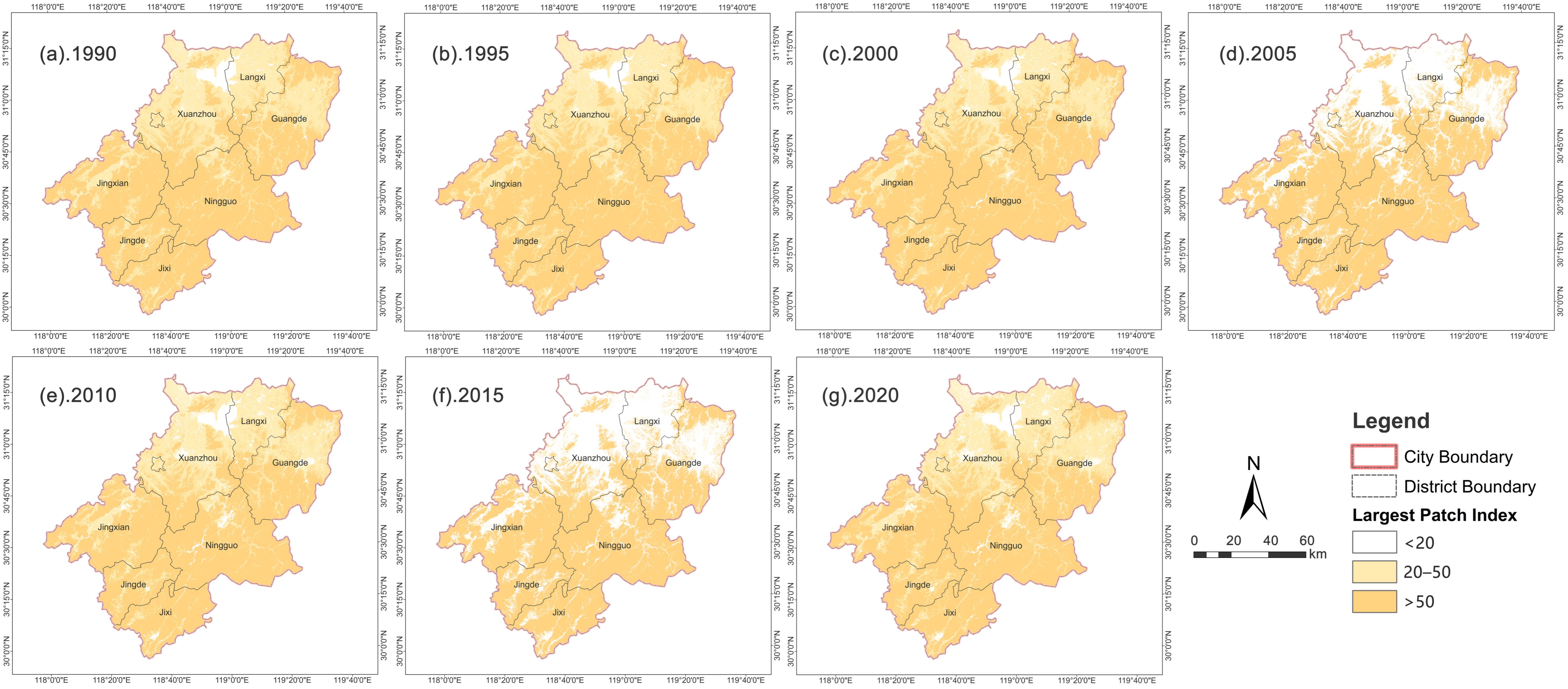
LPI displayed a distinct south-high to north-low spatial gradient. Southern deep-mountain counties (Jixi, Jingde, Jingxian) featured large contiguous forest patches, with LPI values persistently above 50. Subject to cultivated land segmentation and urban expansion pressures, northern plain and hilly county LPI values generally fell below 20 (Figure 7). Low-value zones surrounding northern towns fluctuated synchronously with urban expansion and land consolidation cycles, while southern high-value domains remained spatially stable.

Figure 7. Spatial distribution of the largest patch index (LPI) in Xuancheng City, 1990–2020.

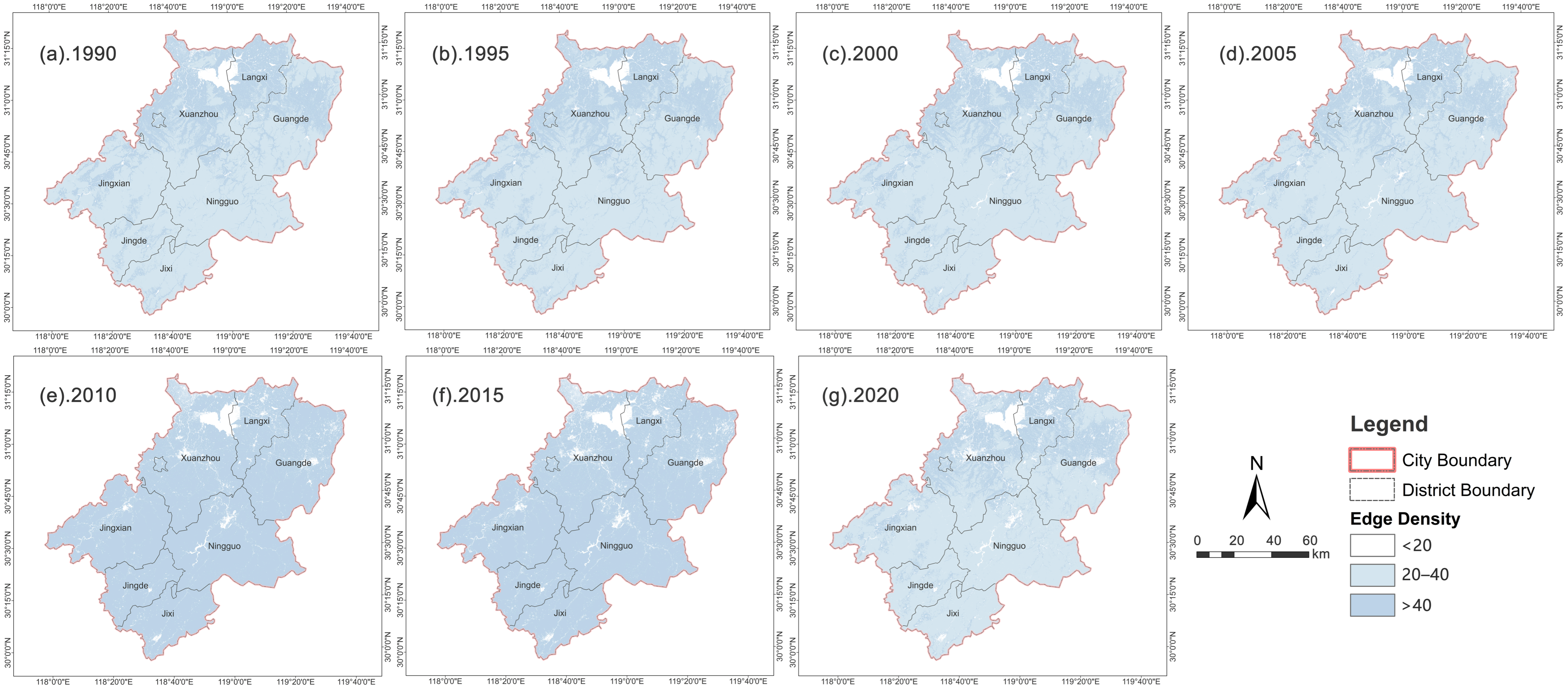
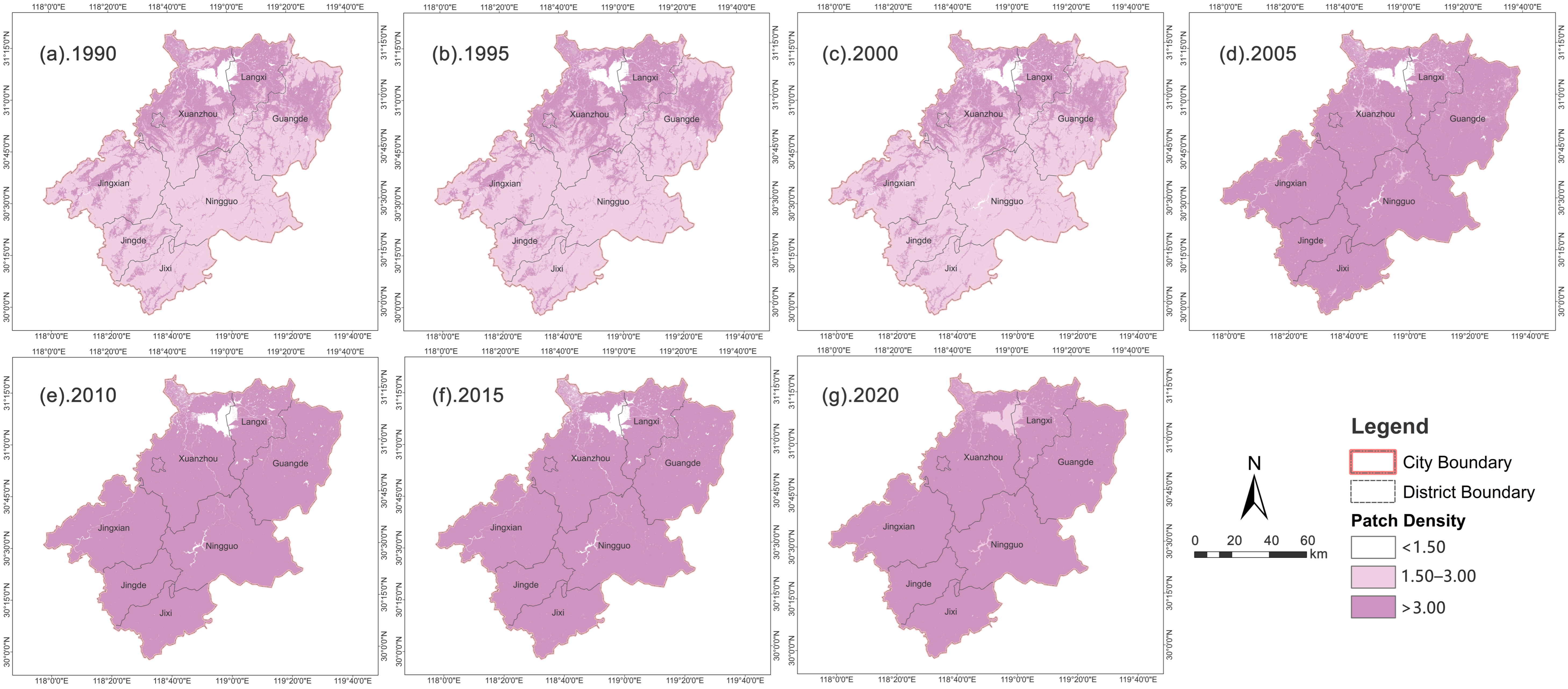
ED maintained stable spatial patterns: high-value clusters concentrated across suburban zones, while southwestern deep-mountain areas sustained low-value conditions (Figure 8). PD exhibited gradual southward propagation: high-value domains predominated across northern plains in 1990 and progressively spread toward central-eastern suburban belts and southwestern mountain hinterlands, compressing north–south magnitude disparities. After 2015, outward-oriented expansion decelerated substantially under territorial spatial management policy frameworks (Figure 9).

Figure 8. Spatial distribution of edge density (ED) in Xuancheng City, 1990–2020.

Figure 9. Spatial distribution of patch density (PD) in Xuancheng City, 1990–2020.

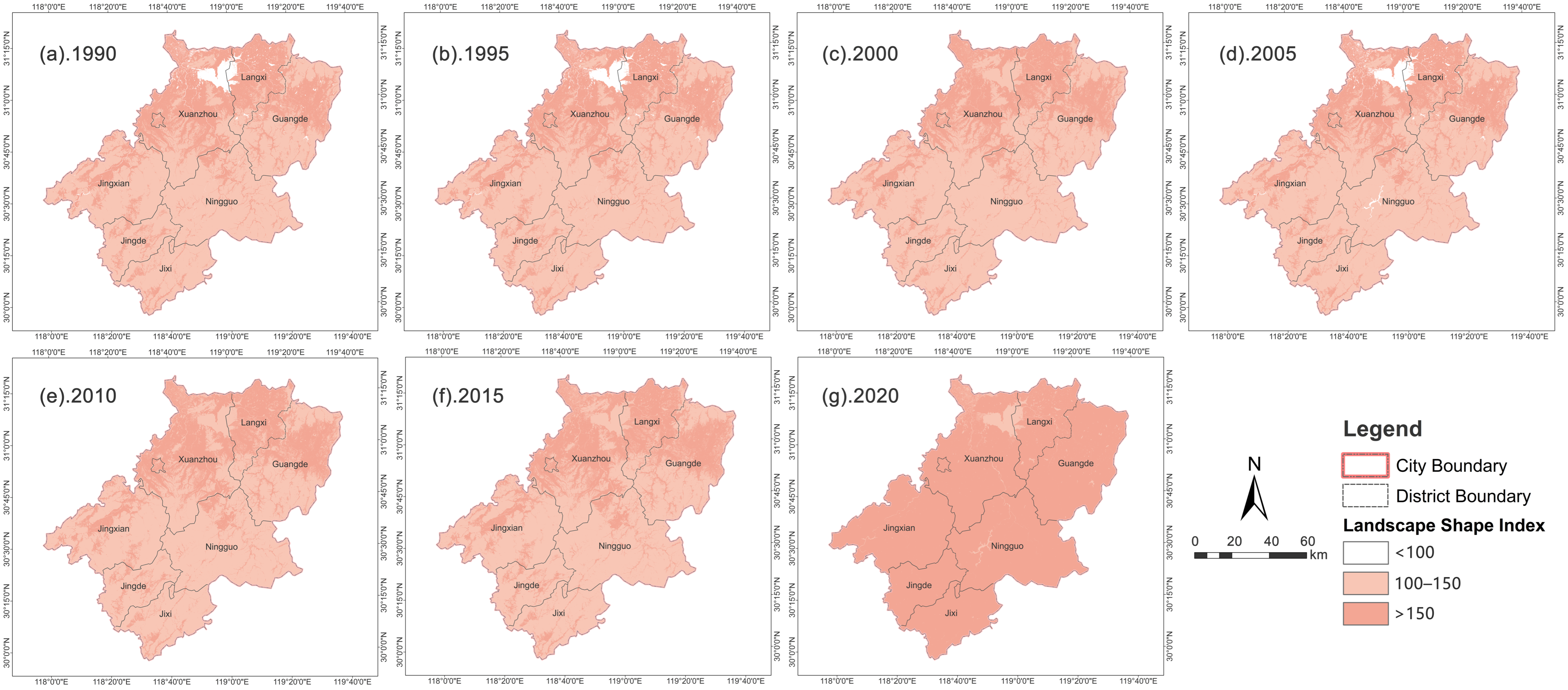
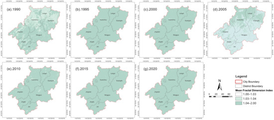
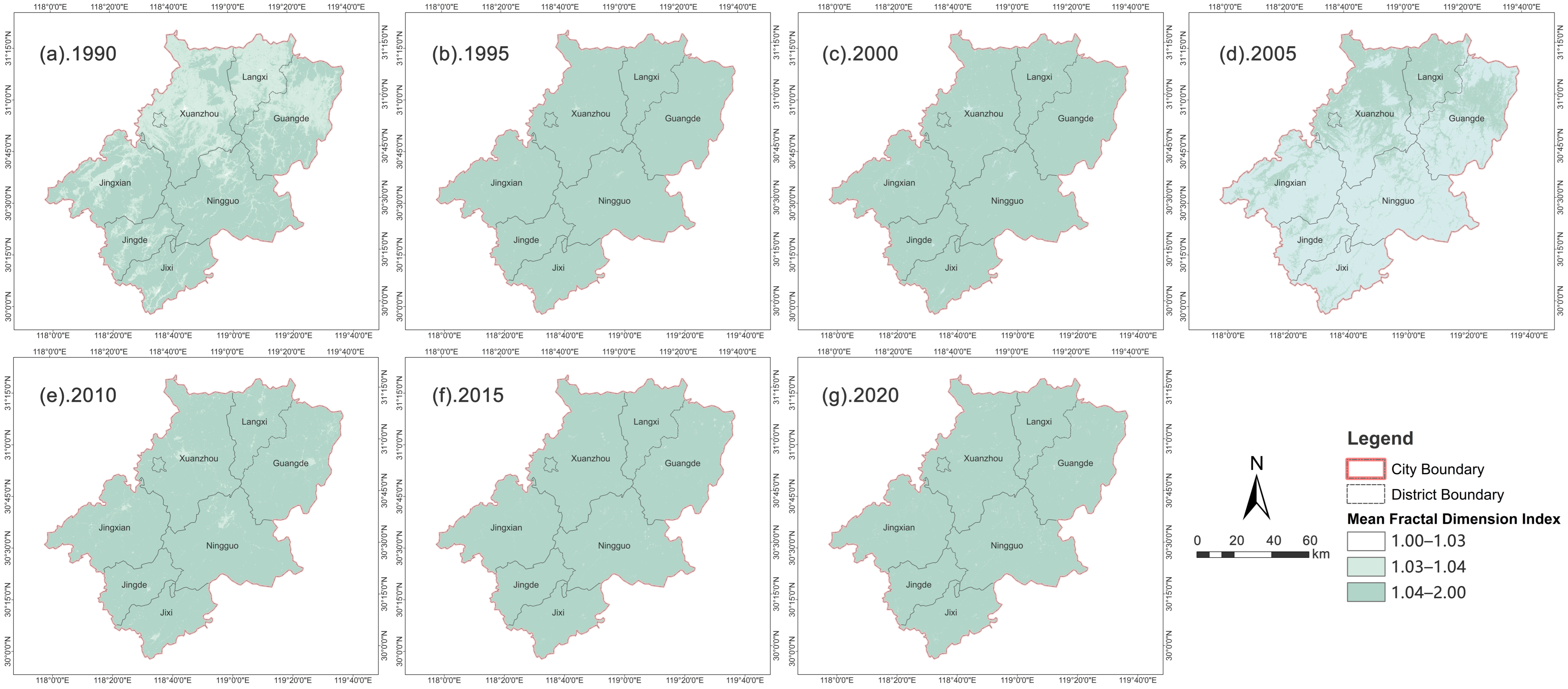
LSI exhibited north-high and south-low spatial patterning. High-value zones clustered within the northern main urban district and central-eastern transportation corridors, whereas southern native forest terrain maintained relatively regular patch geometries (Figure 10). Over time, high-value domains progressively extended into hilly zones and alongside transport routes. Constrained by natural topographic conditions, FRAC_MN consistently yielded higher values for southern mountain terrain relative to northern plains, though this north–south discrepancy gradually diminished (Figure 11).

Figure 10. Spatial distribution of the landscape shape index (LSI) in Xuancheng City, 1990–2020.

Figure 11. Spatial distribution of the mean fractal dimension index (FRAC_MN) in Xuancheng City, 1990–2020.

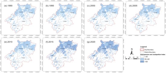
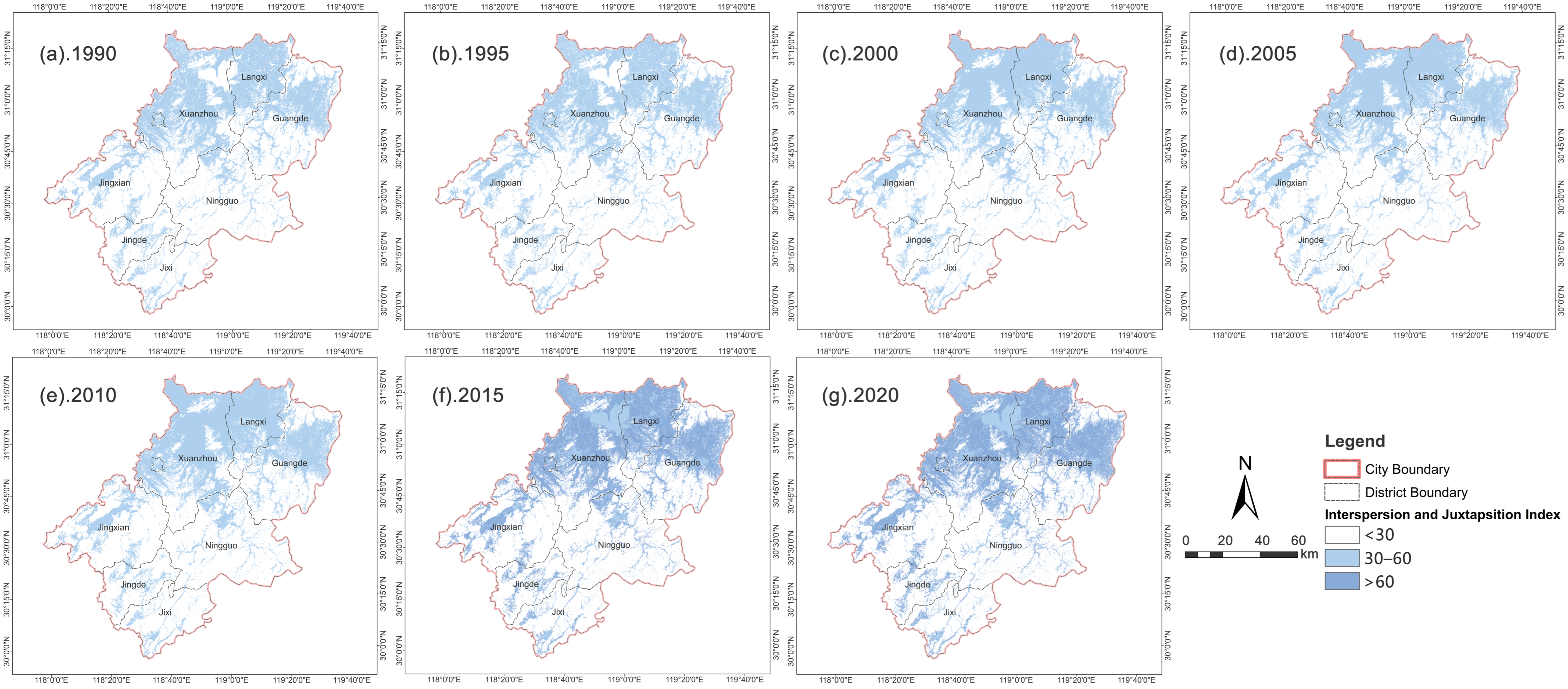
IJI demonstrated north-high and south-low spatial behavior (Figure 12). Urban–rural ecotone zones possessed the highest land use intermixing; northern agricultural plains exhibited moderate index magnitudes; southern contiguous forest terrain maintained high landscape homogeneity. High-value mixed land use zones evolved from sporadic suburban county hotspots toward progressive northward diffusion aligned with transportation corridors. By 2020, continuous medium-to-high interspersion domains had formed across northern plains; landscape mosaicism had become the dominant regional structural signature.

Figure 12. Spatial distribution of the interspersion and juxtaposition index (IJI) in Xuancheng City, 1990–2020.

3.3. Temporal and Spatial Evolution of Land Use Carbon Emissions

3.3.1. Characteristics of Temporal Evolution

Land use carbon emissions increased 15.65-fold from 1990 through 2020, following a three-stage temporal trajectory: slow growth (1990–2000), rapid escalation (2000–2015), and high-level decline (2015–2020) (Table 10). Built-up areas contributed over 98% of total emission increments. Forests functioned as the primary carbon sink; other land use categories exerted only marginal sink/source effects.

Table 10. Changes in land use carbon emissions in Xuancheng City, 1990–2020 (unit: t).

Year CE	Cultivated Land	Forest	Grassland	Water	Built-Up Area	Unutilized Land	Total
1990	197,850.85	−454,567.68	−60.39	−9599.51	359,276.14	0.00	92,899.42
1995	196,258.02	−456,428.98	−36.67	−9471.41	418,321.81	0.00	148,642.77
2000	178,207.75	−469,504.81	−57.83	−10,033.34	800,037.48	−0.01	498,649.24
2005	175,877.46	−466,028.18	−123.39	−10,030.49	1,072,700.13	−0.02	772,395.52
2010	175,836.78	−460,357.01	−90.93	−10,505.59	1,415,866.14	−0.01	1,120,749.38
2015	172,284.15	−452,555.67	−157.64	−11,430.53	1,910,894.56	−0.10	1,619,034.77
2020	177,467.45	−445,633.98	−230.70	−11,490.46	1,826,600.13	−0.63	1,546,711.80

3.3.2. Characteristics of Spatial Differentiation

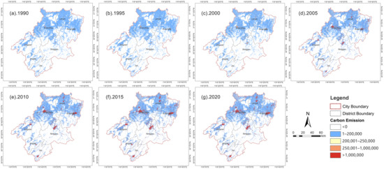
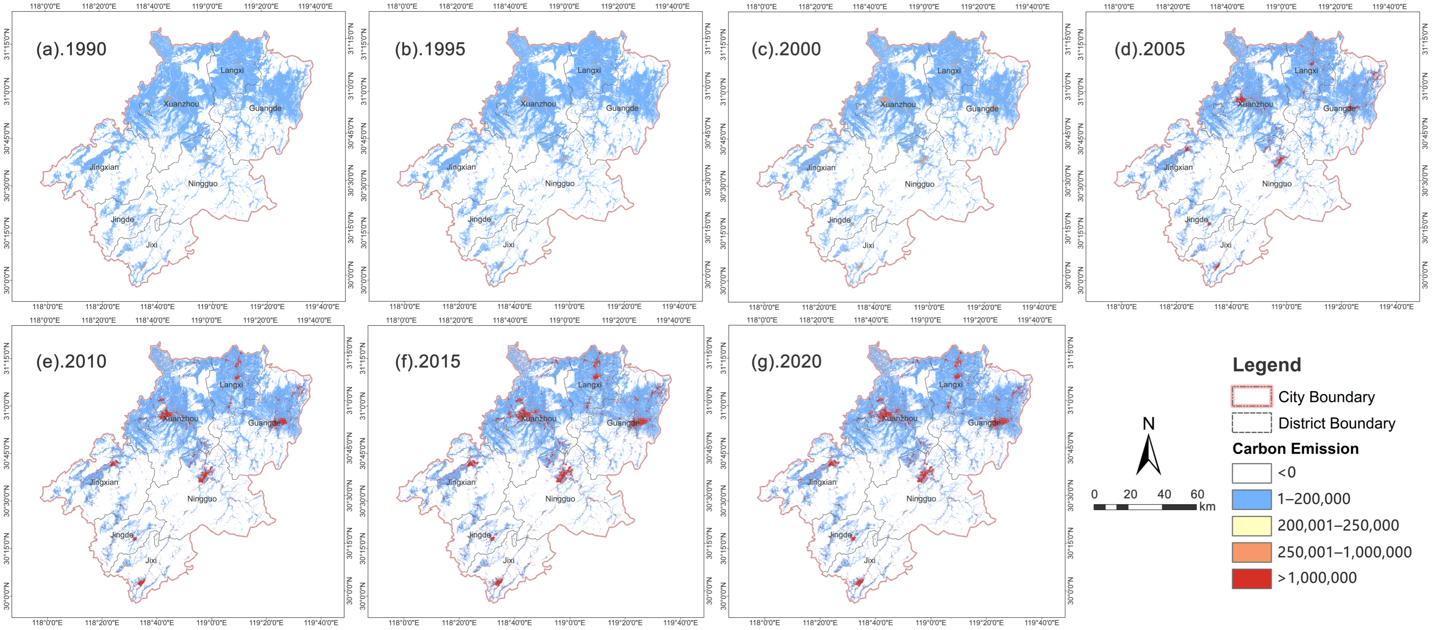
Carbon emission spatial distributions closely mirrored land use spatial configurations, presenting a north-high–south-low pattern, featuring one primary plus two secondary emission hotspots and gradient magnitude decay extending outward from transportation corridors (Figure 13). Southern contiguous forest terrain formed stable carbon sink zones. Northern plains constituted medium-to-low emission transition belts. The urban zones of Xuanzhou, Ningguo, and Guangde represented high-emission cores forming bead-shaped spatial extensions aligned with transportation corridors. High-emission zones experienced four-stage spatial evolution: sporadic emergence, axial expansion, peak-period proliferation, and moderate contraction, synchronized with urban development trajectories. After 2015, both emission intensity and spatial coverage diminished, documenting measurable regulatory policy impacts.

Figure 13. Spatial distribution of land use carbon emissions in Xuancheng City, 1990–2020.

3.4. Correlation Analysis Between Landscape Pattern and Carbon Emissions

Excluding unutilized land (negligible areal coverage and invalid metric outputs), five land use classes together with six core landscape pattern metrics were incorporated within the combined Spearman correlation plus grey relational analysis analytical workflow.

3.4.1. Correlation Direction and Significance

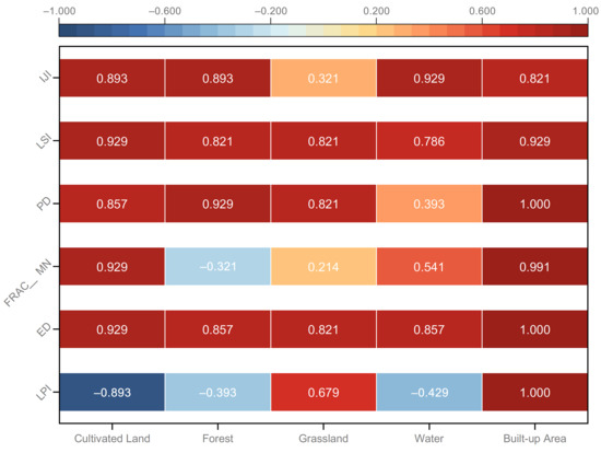
Spearman correlation outputs (Figure 14, Appendix A Table A10) reveal substantial land use-class heterogeneity. All built-up area metrics returned statistically significant positive correlations against carbon emissions; LPI, ED, and PD achieved highly significant correlation magnitudes. This demonstrates that contiguous expansion of core built-up area patches constitutes the primary factor associated with rising carbon emission outputs. Cultivated land metric responses displayed bidirectional divergence: LPI yielded negative correlation coefficients, whereas fragmentation- and morphology-related metrics produced positive correlations, reflecting synergistic effects associated with built-up area encroachment onto cultivated land resources. Most morphological and configurational metrics for forest, grassland, and water categories returned significant positive correlations; scale-related metrics failed to achieve significance. This outcome illustrates that ecological space fragmentation proceeds synchronously with built-up area encroachment, while ecological land areal scale exerts only marginal impacts on aggregate regional emission totals.

Figure 14. Heatmap of Spearman correlation coefficients between landscape pattern indexes and carbon emissions for each land use type.

3.4.2. Correlation Intensity and Driving Hierarchy

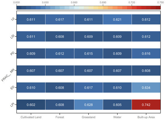
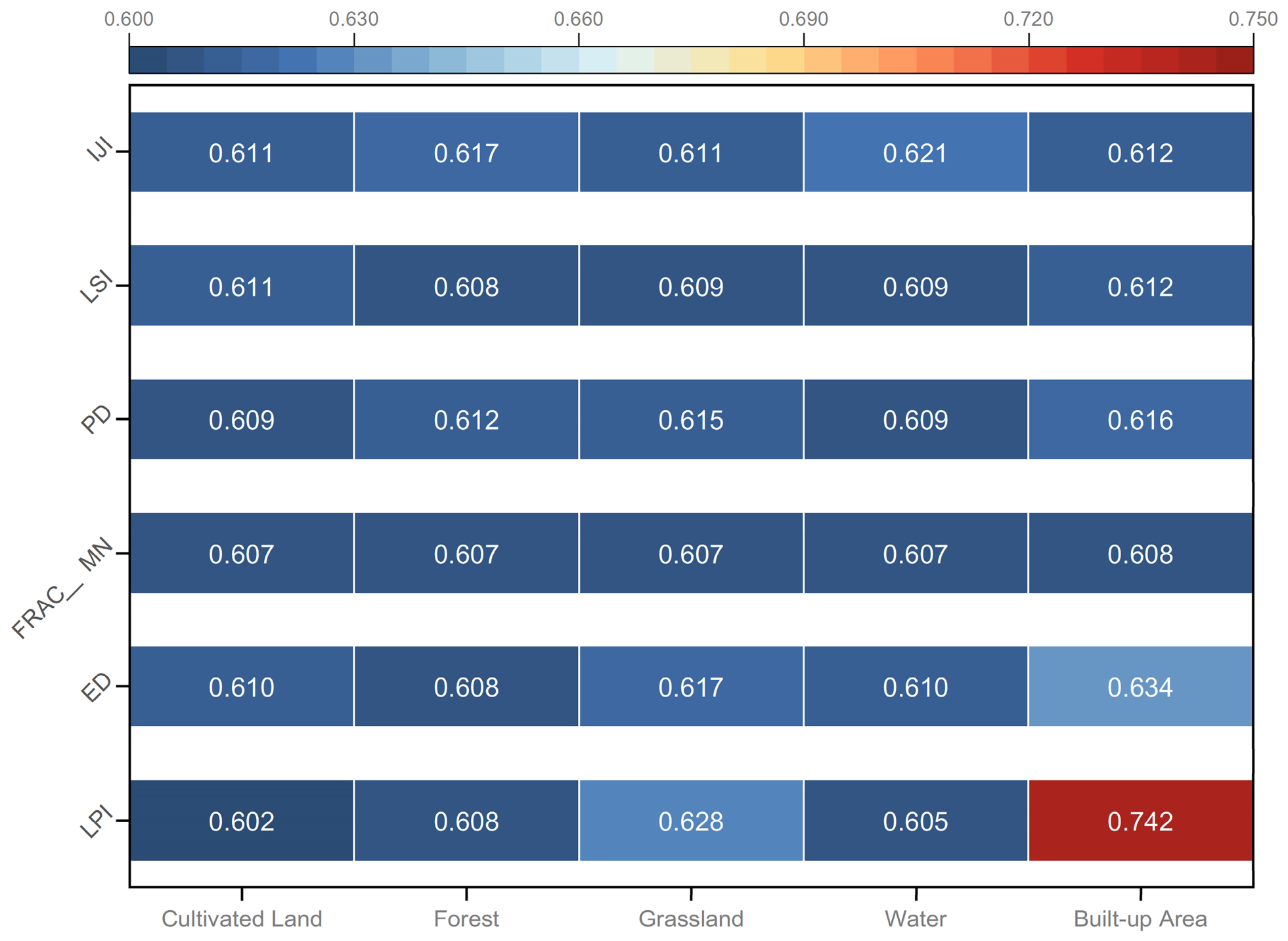
Grey relational analysis outputs (Figure 15) yielded relational degree values spanning 0.602–0.742, indicating moderate-to-strong synergistic temporal covariation. Built-up area LPI returned the highest grey relational magnitude (0.742), representing the sole factor attaining the strong-correlation tier. This points toward a driving system configuration defined by single core dominance supplemented by multi-factor auxiliary effects.

Figure 15. Heatmap of grey relational degrees between landscape pattern indices and total regional carbon emissions for each land use type.

As the dominant regional carbon source, built-up area pattern modifications exhibit direct associations with carbon emission dynamics. Patch-scale magnitude and patch contiguity exert far stronger correlative influence compared with edge morphology, fragmentation, or spatial configuration attributes. For the remaining four land use classes, observed correlations more likely represent synergistic accompanying covariation during land use conversion events rather than independent causal mechanisms.

Scale-associated metrics exhibited pronounced land use-class-specific divergence. Built-up area scale and contiguity indicators showed strong positive covariation with carbon emissions, whereas ecological and agricultural land categories returned opposite direction and weaker magnitude responses. Morphology- and fragmentation-related metrics produced relatively consistent effect magnitudes across land use classes. Spatial configuration metrics demonstrated relative temporal stability and constitute secondary optimization targets for low-carbon landscape governance. Based on rank-ordered correlation intensities, only built-up area LPI falls within the core-dominant driver tier.

4. Discussion

4.1. Comparison with Previous Studies

The finding that the LPI of built-up areas possesses the strongest correlation with carbon emissions aligns with studies in plain urban agglomerations [1,11,13]. This cross-context consistency supports the view that positive covariation between contiguous built-up area expansion and carbon emission outputs reflects a fundamental mechanism: compact urban cores concentrate energy consumption and industrial activity intensities [36,49]. Nevertheless, effect magnitudes differ substantially between plain city versus hilly city contexts. Within plain terrain cities, ED exerts weaker correlative influence relative to LPI because concentric outward expansion maintains relatively regular urban patch perimeters [10,12]. In Xuancheng, valley topography confines urban growth to axial strips aligned with transportation corridors, markedly amplifying ED-related correlation magnitudes. This terrain-modulated modulating mechanism has been insufficiently documented in prior research based on flat-terrain case-study samples [3,50]. Accordingly, this study supplies empirical evidence demonstrating that topographic conditions fundamentally reshape the relative importance of landscape metrics for carbon regulation outcomes.

The results additionally refine understanding regarding the transferability of the compact city theory. In plain cities, compact spatial configurations lower per-capita emissions by enhancing public transit operational efficiency [10,36]. Within hilly region Xuancheng, compact spatial agglomeration emerges as a passive outcome imposed by topographic constraints rather than deliberate planning interventions, coinciding with energy intensive industries clustered along limited transportation corridors [23,37]. Consequently, compactness does not automatically translate into emission reduction benefits, implying that the compact city theory cannot be directly extrapolated to hilly region contexts without accounting for local industrial structure and socioeconomic development stage [38,39]. Regarding ecological land variables: although improved connectivity and patch integrity substantially strengthen carbon sequestration performance within ecologically fragile settings [25,47], the marginal contributions of ecological land connectivity to aggregate carbon emission totals remain negligible within Xuancheng. Built-up area-driven emissions dominate regional carbon budgets, accounting for over 98% of total emission increments. Analogous patterns have been documented for the Beijing–Tianjin–Hebei region [3,32] and the Yangtze Economic Belt [24].

4.2. Applicability and Limitations of the Combined Analytical Method

This two-step analytical framework integrating Spearman correlation plus grey relational analysis proves suitable for small-sample time-series datasets. With merely seven time-point observations, robust regression model fitting is infeasible. Spearman correlation delivers statistical significance screening; GRA ranks relative factor influence magnitudes without imposing data-distribution assumptions. Note that this combined descriptive framework cannot establish causal relationships.

Small sample sizes inherently constrain statistical power. Temporal observations also suffer from temporal autocorrelation, effectively reducing the number of statistically independent data points. Given the volume of landscape metric and land use class combinations evaluated (approximately 30 total), the possibility of chance-driven significant outcomes cannot be fully excluded. Exact p-values for all Spearman correlation outputs are supplied within Appendix A Table A10 to support contextualized significance evaluation by readers.

A further key limitation arises from the carbon accounting workflow: emissions are computed as land use area multiplied by fixed coefficient values. Accordingly, strong correlations between built-up area landscape metrics and aggregate carbon emissions may partially stem from their shared dependence on built-up area expansion. Per-unit-area emission intensity increased only modestly (roughly 8.5%) over the full 30-year interval, whereas aggregate carbon emissions expanded 15.65-fold. Area expansion, rather than landscape-morphological attributes, constituted the primary driver of emission growth. Observed associations should therefore be interpreted as temporal covariation instead of definitive proof that landscape morphology independently drives carbon emission magnitudes.

Additionally, 30 m resolution land use datasets cannot fully capture fine-scale edge feature detail; the analysis is restricted exclusively to temporal domain evaluation without examining spatial interaction effects; carbon emission coefficients carry intrinsic parameter uncertainty. Future research could deploy higher resolution remote sensing imagery, spatially explicit process-based models, and energy-statistic-driven direct-emission measurements to mitigate these limitations.

5. Conclusions

This study investigated linkages between landscape pattern evolution and carbon-emission dynamics within Xuancheng, a representative hilly region city, using multi-temporal land use datasets spanning 1990–2020. The LPI of built-up areas exhibited the strongest temporal covariation with carbon emission outputs, followed sequentially by ED and PD with progressively weaker correlative magnitudes. Cultivated land and forest metrics display only synchronous accompanying covariation, lacking independent causal explanatory capacity. Valley terrain constraints confine urban expansion to axial strips aligned with transportation corridors, elevating correlation magnitudes for edge-related landscape metrics. This outcome generates divergent carbon outcomes associated with compact spatial agglomeration between hilly and plain terrain cities and delineates contextual boundary conditions for the compact city theory. For small-sample long-term time-series datasets, the combined Spearman-GRA workflow delivers a viable descriptive framework for identifying factor influence hierarchies, while outputs remain exploratory in nature.

Based on these empirical outcomes, targeted low-carbon spatial governance recommendations are proposed: restrain uncontrolled contiguous built-up area sprawl; establish landscape metric threshold benchmarks aligned with urban development boundaries; regularize built-up area boundary morphologies; strengthen green corridors and green wedges to sustain stable regional carbon sink performance; and implement spatially differentiated governance schemes. Northern urban-focused zones should prioritize improvements in land use utilization intensity; central transition zones ought to constrain scattered patch-oriented development; southern ecological conservation zones must preserve large contiguous natural forest patch systems.

References

- Tang, Z.; Wang, Y.; Fu, M.; Xue, J. The role of land use landscape patterns in the carbon emission reduction: Empirical evidence from China. Ecol. Indic. 2023, 156, 111176. [Google Scholar] [CrossRef] [Scilit]
- Zhang, J.; Roosli, R. Deciphering land use carbon emissions through landscape pattern changes: A case study of the Urban Agglomeration in the Middle Reaches of the Yangtze River. Environ. Dev. Sustain. 2025, 16, 1–28. [Google Scholar] [CrossRef] [Scilit]
- Li, A.; Yin, X.; Wei, H. Spatiotemporal Evolution and Driving Factors of the Relationship Between Land Use Carbon Emissions and Ecosystem Service Value in Beijing-Tianjin-Hebei. Land 2025, 14, 1698. [Google Scholar] [CrossRef] [Scilit]
- Zhao, C.; Liu, Y.; Yan, Z. Effects of land-use change on carbon emission and its driving factors in Shaanxi Province from 2000 to 2020. Environ. Sci. Pollut. Res. 2023, 30, 68313–68326. [Google Scholar] [CrossRef] [Scilit] [PubMed]
- Lin, Q.; Zhang, L.; Qiu, B.; Zhao, Y.; Wei, C. Spatiotemporal Analysis of Land Use Patterns on Carbon Emissions in China. Land 2021, 10, 141. [Google Scholar] [CrossRef] [Scilit]
- Meng, J.; Wang, C.; Zou, Y.; Han, Z.; Zou, G. Multi-scale spatiotemporal interactions between land use transformation and carbon emissions in China from 1980 to 2020. Resour. Conserv. Recycl. 2026, 226, 108653. [Google Scholar] [CrossRef] [Scilit]
- Wang, X.; Zhao, X.; Zhang, S.; Shi, S.; Zhang, X. Decoupling Effect and Driving Factors of Land-Use Carbon Emissions in the Yellow River Basin Using Remote Sensing Data. Remote Sens. 2023, 15, 4446. [Google Scholar] [CrossRef] [Scilit]
- Zhao, T.; Zhou, X.; Jian, Z.; Zhu, J.; Liu, M.; Yin, S. Spatial-Temporal Evolution and Influencing Factors of Land-Use Carbon Emissions: A Case Study of Jiangxi Province. Appl. Sci. 2025, 15, 10986. [Google Scholar] [CrossRef] [Scilit]
- Chen, M.; Yan, Z.; Zhang, J.; Xue, Z. Analysis of Spatio-Temporal Dynamics and Determinants of Land Use Carbon Emissions in Jiangsu Province, China. Land 2025, 14, 905. [Google Scholar] [CrossRef] [Scilit]
- Ou, Y.; Bao, Z.; Ng, S.; Song, W.; Chen, K. Land-use carbon emissions and built environment characteristics: A city-level quantitative analysis in emerging economies. Land Use Policy 2024, 137, 107019. [Google Scholar] [CrossRef] [Scilit]
- Zeng, X.; Fan, D.; Zheng, Y.; Li, S. Exploring the Differentiated Impact of Urban Spatial Form on Carbon Emissions: Evidence from Chinese Cities. Land 2024, 13, 874. [Google Scholar] [CrossRef] [Scilit]
- Han, X.; Fu, M.; Huang, X. Spatiotemporal Heterogeneity of Land-Use Landscape Pattern Effects on CO2 Emissions at the City-Level Scale in China. Land 2025, 14, 1715. [Google Scholar] [CrossRef] [Scilit]
- Liu, C.; Chen, G.; Li, H.; Li, J.; Muga, G. Impact of Urban Morphology on Carbon Emission Differentiation at County Scale in China. Land 2025, 14, 1163. [Google Scholar] [CrossRef] [Scilit]
- Liu, Q.; Qiao, J.; Han, D.; Li, M.; Shi, L. Spatiotemporal Evolution of Cultivated Land Use Eco-Efficiency and Its Dynamic Relationship with Landscape Pattern Change from the Perspective of Carbon Effect: A Case Study of Henan, China. Agriculture 2023, 13, 1350. [Google Scholar] [CrossRef] [Scilit]
- Cao, W.; Zhou, W.; Wu, T.; Wang, X.; Xu, J. Spatial-temporal characteristics of cultivated land use eco-efficiency under carbon constraints and its relationship with landscape pattern dynamics. Ecol. Indic. 2022, 141, 109140. [Google Scholar] [CrossRef] [Scilit]
- Sun, Y.; Zhi, J.; Han, C.; Xue, C.; Zhao, W.; Liu, W.; Bao, S. The Impact of Future Land Use Change on Carbon Emission and Its Optimization Strategy. Forests 2024, 15, 1292. [Google Scholar] [CrossRef] [Scilit]
- Hu, J.; Song, M.; Zhang, L. Spatial and temporal evolution of land use carbon emission and carbon balance zoning: Evidence from Xinjiang China. Sci. Rep. 2025, 15, 35705. [Google Scholar] [CrossRef] [Scilit] [PubMed]
- Li, S.; Sun, Z.; Wen, R.; Yang, H.; Li, J.; Chen, T.; Zheng, Y.; Zhu, N. Spatiotemporal patterns and the influence mechanism of urban landscape pattern on carbon emission performance: Evidence from Chinese cities. Sustain. Cities Soc. 2025, 118, 106042. [Google Scholar] [CrossRef] [Scilit]
- Wu, Z.; Zhou, L.; Wang, Y. Prediction of the Spatial Pattern of Carbon Emissions Based on Simulation of Land Use Change under Different Scenarios. Land 2022, 11, 1788. [Google Scholar] [CrossRef] [Scilit]
- Fan, H.; Jin, X.; Zhu, J.; Zhang, Z.; Hu, C.; Hu, H.; Du, X.; Zhou, Y. Differentiated landscape pattern transformation strategies drive territorial space carbon neutrality: A path exploration based on mixed land use units. Sustain. Cities Soc. 2025, 133, 106865. [Google Scholar] [CrossRef] [Scilit]
- Hu, J.; Du, Y.; Ma, Y.; Liu, D.; Yu, J.; Miao, Z. Exploring the Spatiotemporal Impact of Landscape Patterns on Carbon Emissions Based on the Geographically and Temporally Weighted Regression Model: A Case Study of the Yellow River Basin in China. Sustainability 2025, 17, 9140. [Google Scholar] [CrossRef] [Scilit]
- Pan, B.; Wang, Q.; Diao, Z.; Li, J.; Liu, W.; Gao, Q.; Shu, Y.; Du, J. Landscape Patterns and Carbon Emissions in the Yangtze River Basin: Insights from Ensemble Models and Nighttime Light Data. Atmosphere 2025, 16, 1173. [Google Scholar] [CrossRef] [Scilit]
- Yang, Y.; Yang, M.; Zhao, B.; Lu, Z.; Sun, X.; Zhang, Z. Spatially explicit carbon emissions from land use change: Dynamics and scenario simulation in the Beijing-Tianjin-Hebei urban agglomeration. Land Use Policy 2025, 150, 107473. [Google Scholar] [CrossRef] [Scilit]
- Jiang, X.; Chu, X.; Yang, X.; Jiang, P.; Zhu, J.; Cai, Z.; Yu, S. Spatiotemporal Dynamics of Land Use Carbon Balance and Its Response to Urbanization: A Case of the Yangtze River Economic Belt. Land 2025, 14, 41. [Google Scholar] [CrossRef] [Scilit]
- Zhao, Y.; Ning, S.; Yan, A.; Jiang, P.; Ren, H.; Li, N.; Huo, T.; Sheng, J. Analysis of Carbon Emissions and Ecosystem Service Value Caused by Land Use Change, and Its Coupling Characteristics in the Wensu Oasis, Northwest China. Agronomy 2025, 15, 2307. [Google Scholar] [CrossRef] [Scilit]
- Cui, J.; Wei, Z.; Li, X.; Yuan, C.; Liu, L.; Zhang, D. An integrated land use-carbon modeling framework for net carbon emissions and spatial optimization in Northeast China. J. Clean Prod. 2025, 525, 146545. [Google Scholar] [CrossRef] [Scilit]
- Li, Y.; Peng, Y.; Cheng, W.; Peng, H. Spatial-temporal evolution and multi-scenario prediction of carbon emissions from land use in the adjacent areas of nature reserves. Ecol. Indic. 2025, 170, 113047. [Google Scholar] [CrossRef] [Scilit]
- Zhang, Y.; Li, J.; Liu, S.; Zhou, J. Spatiotemporal Effects and Optimization Strategies of Land-Use Carbon Emissions at the County Scale: A Case Study of Shaanxi Province, China. Sustainability 2024, 16, 4104. [Google Scholar] [CrossRef] [Scilit]
- Nie, X.; Wang, C.; Li, K.; Huang, W. Grid-Based Analysis of the Spatial Relationships and Driving Factors of Land-Use Carbon Emissions and Landscape Ecological Risk: A Case Study of the Hexi Corridor, China. Land 2026, 15, 669. [Google Scholar] [CrossRef] [Scilit]
- Pu, X.; Cheng, Q.; Chen, H. Spatial-temporal dynamics of land use carbon emissions and drivers in 20 urban agglomerations in China from 1990 to 2019. Environ. Sci. Pollut. Res. 2023, 30, 107854–107877. [Google Scholar] [CrossRef] [Scilit] [PubMed]
- Zhao, L.; Yang, C.; Zhao, Y.; Wang, Q.; Zhang, Q. Spatial Correlations of Land Use Carbon Emissions in Shandong Peninsula Urban Agglomeration: A Perspective from City Level Using Remote Sensing Data. Remote Sens. 2023, 15, 1488. [Google Scholar] [CrossRef] [Scilit]
- Lv, W.; Xie, Y.; Zeng, P. Assessing and Predicting Spatiotemporal Alterations in Land-Use Carbon Emission and Its Implications to Carbon-Neutrality Target: A Case Study of Beijing-Tianjin-Hebei Region. Land 2024, 13, 2066. [Google Scholar] [CrossRef] [Scilit]
- Yuan, D.; Zhang, L.; Fan, Y.; Yang, R. Investigating spatio-temporal variations and contributing factors of land use-related carbon emissions in the Beijing-Tianjin-Hebei Region, China. Sci. Rep. 2024, 14, 18976. [Google Scholar] [CrossRef] [Scilit] [PubMed]
- Li, K.; Wang, H.; Zhang, X.; Su, H.; Xu, J.; Hua, X. Assessing the divergent effects of green infrastructure landscape patterns on carbon emission and sequestration in 31 cities across China. Build. Environ. 2025, 280, 113110. [Google Scholar] [CrossRef] [Scilit]
- Bian, R.; Zhao, A.; Zou, L.; Liu, X.; Xu, R.; Li, Z. Simulation and Prediction of Land Use Change and Carbon Emission under Multiple Development Scenarios at the City Level: A Case Study of Xi’an, China. Land 2024, 13, 1079. [Google Scholar] [CrossRef] [Scilit]
- Wu, H.; Fang, S.; Zhang, C.; Hu, S.; Nan, D.; Yang, Y. Exploring the impact of urban form on urban land use efficiency under low-carbon emission constraints: A case study in China’s Yellow River Basin. J. Environ. Manag. 2022, 311, 114866. [Google Scholar] [CrossRef] [Scilit] [PubMed]
- Jiang, P.; Wen, C.; Ma, Z.; Dai, F. Spatiotemporal dynamics and planning responses to address carbon balance and land-use mixtures in megacities: A case study of Wuhan, China. Environ. Impact Assess. Rev. 2026, 116, 108139. [Google Scholar] [CrossRef] [Scilit]
- Huo, J.; Shi, Z.; Zhu, W.; Yan, Y.; Xue, H. Carbon neutral spatial zoning and optimization based on land use carbon emission in the qinba mountain region, China. Sci. Rep. 2025, 15, 1032. [Google Scholar] [CrossRef] [Scilit] [PubMed]
- Zhang, Y.; Tang, J.; Hu, X.; Chen, C.; Luo, Z.; Li, Q.; Li, Q. Understanding the Spatiotemporal Patterns and Drivers of Carbon Stock in Central-Southern China’s Hilly Regions Through Land Use Change and Scenario Simulation. Sustainability 2025, 17, 5578. [Google Scholar] [CrossRef] [Scilit]
- Wang, Q.; Yang, C.; Wang, M.; Zhao, L.; Zhao, Y.; Zhang, Q.; Zhang, C. Decoupling analysis to assess the impact of land use patterns on carbon emissions: A case study in the Yellow River Delta efficient eco-economic zone, China. J. Clean Prod. 2023, 412, 137415. [Google Scholar] [CrossRef] [Scilit]
- Alshehri, F.; Abuamarah, B.; Abd El-Hamid, H. Impact of land use dynamics on land surface temperature using optical remote sensing data integrated with statistical analysis in Riyadh, Saudi Arabia. Adv. Space Res. 2023, 72, 1739–1750. [Google Scholar] [CrossRef] [Scilit]
- Talebi Khiavi, H.; Mostafazadeh, R.; Asaadi, M.A.; Asbaghian Namini, S.K. Temporal land use change and its economic values under competing driving forces in a diverse land use configuration. Arab. J. Geosci. 2022, 15, 1597. [Google Scholar] [CrossRef] [Scilit]
- Zheng, Y.W.; Wang, Z.F.; Li, S.J.; Zheng, Z.Y.; Wang, F.; Zhao, X.H.; He, J.N.; Ji, D.S.; Wang, W.K. Analysis of Spatiotemporal Dynamic Evolution Characteristics and Driving Forces of Land Use/Cover Change in the Weihe River Basin in the Past 30 Years. Huanjing Kexue 2025, 46, 7106–7118. [Google Scholar] [CrossRef] [Scilit] [PubMed]
- Chen, W.; Ye, X.; Li, J.; Fan, X.; Liu, Q.; Dong, W. Analyzing requisition-compensation balance of farmland policy in China through telecoupling: A case study in the middle reaches of Yangtze River Urban Agglomerations. Land Use Policy 2019, 83, 134–146. [Google Scholar] [CrossRef] [Scilit]
- Bi, Y.; Zuo, D.; Song, Y.; Xu, Z.; Wang, J.; Peng, D.; Pang, B.; Sun, W.; Abbaspour, K.C.; Yang, H. The response of non-point source pollution to land use changes based on the SWAT and PLUS models in an agricultural river basin of Yangtze River, China. J. Hydrol. 2025, 663, 134331. [Google Scholar] [CrossRef] [Scilit]
- Zhou, D.; Xiao, J.; Liu, S.; Huang, L.; Zhang, L.; Fan, J.; Zhao, S. Global impacts of transportation infrastructure on forest degradation and loss. Nat. Commun. 2026, 17, 2339. [Google Scholar] [CrossRef] [Scilit] [PubMed]
- Yu, H.; Hu, X.; Yao, L. Vegetation restoration reduces landscape ecological risk in the Loess Plateau. Geogr. Sustain. 2025, 6, 100320. [Google Scholar] [CrossRef] [Scilit]
- Chen, J.; Li, J.; Li, G.; Zhang, J. How to recognize and characterize land use-based carbon emissions within city networks in the Beijing-Tianjin-Hebei region of China. Urban CLim. 2024, 53, 101789. [Google Scholar] [CrossRef] [Scilit]
- Fang, C.; Wang, S.; Li, G. Changing urban forms and carbon dioxide emissions in China: A case study of 30 provincial capital cities. Appl. Energy 2015, 158, 519–531. [Google Scholar] [CrossRef] [Scilit]
- Zhang, Z.-H.; Xia, N.; Tang, Y.-Q.; Sun, S.-F.; Xu, Z.-J.; Ma, Y.-G. Analysis of the Spatio-temporal Evolution Characteristics and Influencing Factors of Carbon Emissions from Land Use in China at Different Spatial Scales. Huanjing Kexue 2026, 47, 3529–3544. [Google Scholar] [CrossRef] [Scilit] [PubMed]
- Zhang, W.; Xu, H. Effects of land urbanization and land finance on carbon emissions: A panel data analysis for Chinese provinces. Land Use Policy 2017, 63, 493–500. [Google Scholar] [CrossRef] [Scilit]
- Li, W.; Kang, J.; Wang, Y. Exploring the interactions and driving factors among typical ecological risks based on ecosystem services: A case study in the Sichuan-Yunnan ecological barrier area. Ecol. Indic. 2025, 170, 113000. [Google Scholar] [CrossRef] [Scilit]
- Wei, Y.; Li, H.; Zhou, Y.; Commey, N.A.; Jin, J.; Zhou, P. Study on the evolution of regional future drought-flood abrupt alternation events. J. Hydrol. Reg. Stud. 2025, 59, 102459. [Google Scholar] [CrossRef] [Scilit]
- Wei, X.; Wang, Z.; Ding, S.; Liu, S. Stage-Dependent Evolution of Floodplain Landscapes in the Lower Yellow River Under Dam Regulation. Land 2026, 15, 121. [Google Scholar] [CrossRef] [Scilit]
Disclaimer/Publisher’s Note: The statements, opinions and data contained in all publications are solely those of the individual author(s) and contributor(s) and not of MDPI and/or the editor(s). MDPI and/or the editor(s) disclaim responsibility for any injury to people or property resulting from any ideas, methods, instructions or products referred to in the content. |
© 2026 by the authors. Licensee MDPI, Basel, Switzerland. This article is an open access article distributed under the terms and conditions of the Creative Commons Attribution (CC BY) license.