Spatiotemporal Evolution and Multi-Scenario Simulation of Ecosystem Services in the Core Water Source Area of the South-to-North Water Diversion Project’s Middle Route

Abstract

Inter-basin water transfer source areas must sustain local habitat quality while ensuring downstream water security, yet the spatial differentiation mechanisms, driving mechanisms, and scenario-dependent responses of their ecosystem services have not been statistically tested. This study aimed to assess historical changes and future trajectories of ecosystem services in the core water source area of the Middle Route of the South-to-North Water Diversion Project, and established a historical assessment–spatial statistics–driver attribution–scenario projection analytical framework. Five ecosystem services—water yield, soil conservation, nitrogen export, carbon storage, and habitat quality—were quantified using InVEST from 2005 to 2020 and projected to 2050 under SSP126, SSP245, and SSP585 via the PLUS–InVEST coupled model. Spatial patterns were analyzed using Getis–Ord Gi* hot–cold spot analysis, hexagon-based spatial statistics (4.5 km bins), Mantel tests, and the optimal-parameter-based geographical detector. Results show that slope was the dominant spatial driver, exhibiting highly significant Mantel correlations with all five services (p < 0.001), and two-factor interactions consistently exceeded individual factor effects (e.g., population density × temperature: q = 0.527 for habitat quality; slope × temperature: q = 0.516 for soil conservation). Hexagon-based statistics revealed that carbon storage declined substantially from 2005 to 2020 (−3.23%, from 98.75 t/ha to 95.56 t/ha), while water yield and soil conservation showed no pronounced temporal trends. Scenario projections revealed divergent trajectories: relative to the 2020 baseline (267.84 mm), water yield increased by 20.1% under SSP126 (321.86 mm) but declined by 56.3% under SSP585 (117.13 mm); nitrogen export increased under all scenarios; and habitat quality declined continuously to 0.557, 0.546, and 0.539 under SSP126, SSP245, and SSP585, respectively. Within this scenario framework, SSP126 and SSP245 may better support the maintenance of water source ecosystem functions, whereas SSP585 may be associated with greater potential ecological pressures, reflected in lower water yield, higher nitrogen export, and lower habitat quality.

1. Introduction

Inter-basin water transfer source areas are key ecological security regions because their ecosystem conditions directly affect both local environmental stability and downstream water supply. Ecosystem services, such as water regulation, soil retention, nutrient purification, carbon storage, and habitat maintenance, provide the ecological foundation for sustaining water quantity, water quality, and watershed resilience [1,2,3]. However, land-use transformation, climate change, urban expansion, and agricultural intensification have increasingly altered ecosystem structure and function, leading to biodiversity loss, reduced carbon storage, intensified pollution risk, and weakened ecological stability [4,5,6,7,8]. Global observations indicate that over 60% of ecosystems are degrading or being unsustainably exploited, with regulating services experiencing the most significant declines [9]. For water transfer source areas, ecosystem degradation is not only a local environmental issue; it may also weaken water conservation capacity, increase non-point source pollution, reduce habitat quality, and threaten the long-term reliability of clean water delivery. Recent evidence from the Hanjiang River Basin indicates that inter-basin water transfer projects can reshape hydrological–ecological systems across their entire lifecycle, with ecosystem services exhibiting phase-dependent responses [10]. Therefore, clarifying how ecosystem services respond to land-use change and future development pathways is essential for water source protection and sustainable land management.

Research on ecosystem services has evolved from static value accounting to spatially explicit assessment and future scenario simulation. Early studies commonly used equivalent-factor approaches, such as the Xie Gaodi value-equivalent method, to estimate ecosystem service value and support regional ecological compensation [2,11]. With the development of remote sensing, GIS, and ecological models, later studies increasingly quantified specific ecosystem services and revealed their spatiotemporal heterogeneity, trade-offs, and driving mechanisms [12,13,14,15]. More recently, ecosystem service assessment has been linked with land-use simulation, and models such as FLUS, CA-Markov, CLUE-S, and PLUS have been used to evaluate future service changes under alternative development scenarios [16,17,18,19,20]. In addition, Shared Socioeconomic Pathways (SSPs) provide a scenario framework for assessing ecosystem service risks under different climate and socioeconomic development pathways [21,22]. These studies have improved understanding of land use–ecosystem service relationships, but most applications remain focused on ordinary watersheds, urban agglomerations, or general ecological function zones. In the Danjiangkou Reservoir area, existing studies have assessed land use and ecosystem service evolution and their management implications [23], examined ecosystem service supply–demand relationships from a spatial management perspective [24], evaluated conservation priorities through scenario simulation, and documented phase-dependent ecosystem service responses to inter-basin water transfer operations [10]. Collectively, while these studies have advanced understanding of local ecosystem services, they share several limitations: reliance on static or single-model frameworks, absence of integrated spatial statistical diagnostics (e.g., Mantel tests, geographical detectors), lack of SSP-based scenario coupling, and insufficient analysis of ecosystem service trade-offs and synergies. The spatial differentiation mechanisms, driving factor interactions, and scenario-dependent risks of ecosystem services in inter-basin water transfer source areas thus remain insufficiently tested.

The core water source area of the Middle Route of the South-to-North Water Diversion Project represents a typical region facing this challenge. Inter-basin water transfer projects can reshape hydrological, ecological, and socioeconomic systems, making source-area ecosystem stability particularly important [25]. The study area is located in a climate transition zone with strong topographic gradients and high ecological sensitivity. Its forested mountains and hilly areas provide important functions for soil conservation, carbon sequestration, water purification, and habitat maintenance, forming an ecological barrier for “continuous clean water delivery northward” [26]. However, the region also contains cropland- and construction land-dominated plains that are strongly affected by agricultural production, urban expansion, and nitrogen export pressure. This mountain–plain contrast may create spatial mismatches among ecosystem services: forested mountainous areas may maintain strong regulating and supporting services, whereas lowland agricultural and built-up areas may face higher pollution and habitat degradation risks. Such mismatches increase the difficulty of identifying priority areas for ecological protection, land-use regulation, and ecological compensation.

The general objective of this study is to determine how land-use change and future development pathways affect ecosystem service stability and potential ecological pressures in the core water source area. Three research questions are addressed: (1) What were the spatiotemporal patterns of land use and ecosystem services from 2005 to 2020? (2) Which natural and socioeconomic factors dominated the spatial differentiation of ecosystem services, and how did their interactions shape these patterns? (3) How will ecosystem services and potential ecological pressures change by 2050 under different SSP scenarios? We hypothesize that ecosystem services show clear mountain–plain differentiation; that terrain-related natural factors dominate the spatial patterns of regulating and supporting services, while factor interactions further strengthen this differentiation; and that high-emission development pathways are projected to weaken water-related services, increase nitrogen export, and reduce habitat quality, posing higher potential pressures than sustainable pathways. To answer these questions, this study integrates multi-period ecosystem service assessment, spatial clustering analysis, driver attribution, and SSP-based land use–ecosystem service scenario simulation. By coupling the PLUS and InVEST models under SSP-based climate pathways, combining hexagon-based spatial statistics with Mantel tests and geographical detection, and quantifying trade-offs and synergies among ecosystem services, this framework addresses gaps left by previous single-model and static assessments.

This study may advance ecosystem service assessment in three respects. First, coupling PLUS with InVEST under SSP-based climate pathways enables closed-loop simulation from land-use projection to ecosystem service quantification, allowing coherent scenario comparison that single-model approaches cannot achieve. Second, integrating hexagon-based spatial statistics, Mantel tests, and optimal-parameter-based geographical detection could provide a multi-level diagnostic framework that moves beyond conventional correlation or regression to capture spatial heterogeneity, distance-dependent relationships, and factor interactions simultaneously. Third, applying this framework to an inter-basin water transfer source area could address a context where service changes carry dual consequences for local ecological security and downstream water supply reliability—a setting underexamined relative to ordinary watersheds or urban agglomerations. The study identifies where ecosystem services have changed, why they differ spatially, and which future pathways may threaten water source security.

2. Materials and Methods

2.1. Study Area

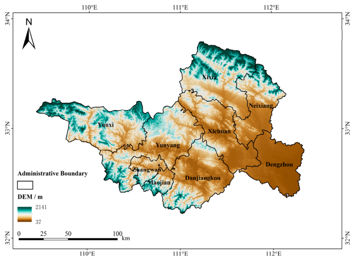
The Middle Route of South-to-North Water Diversion Project is a foundational component of China’s national water network, which alleviates water scarcity in the Huang-Huai-Hai Plain and optimizes regional water resource allocation. Since operation began, the project has transferred over 75 billion cubic meters of water northward, benefiting 27 major cities and approximately 118 million people. The water source area is in the Qinba Mountains of central China (109–112° E, 32–33° N), in the subtropical-to-warm-temperate transition zone. Following the “Notice of the National Development and Reform Commission and the South-to-North Water Diversion Office on Issuing the Counterpart Cooperation Work Plan for the Danjiangkou Reservoir Area and Upstream Regions” (Development and Reform Regional 2013 No. 544), the core water source area includes nine counties (cities, districts): Xichuan County, Xixia County, Dengzhou City, and Neixiang County in Nanyang City, Henan Province; and Zhangwan District, Maojian District, Danjiangkou City (including Wudangshan Special District), Yun County (now Yunyang District), and Yunxi County in Shiyan City, Hubei Province. Total area covers 22,581 km² (Figure 1).

The region has pronounced topographic variation. Terrain descends from northwest to southeast. Mountains and hills dominate. The northern sector (Xixia County) includes the Funiu Mountains, a national nature reserve with high forest coverage. The central and western sectors (Zhangwan District, Maojian District, Danjiangkou City, Yunyang District, Yunxi County) are mostly low mountains and hills vegetated by natural grasslands and planted forests. The eastern sector (Xichuan County, Neixiang County, Dengzhou City) has relatively flat terrain with lower forest coverage, limited environmental capacity, and fragile ecosystems.

2.2. Data Sources

All datasets were obtained from publicly accessible national and international databases and classified as historical or future, and as natural–geographic or socioeconomic data (Table S1). Historical inputs included LULC, DEM, slope, soil, climate, rainfall erosivity, soil erodibility, population density, GDP, roads, and rivers, whereas future inputs included projected LULC, climate, population density, and GDP. Historical LULC, DEM, and slope had a spatial resolution of 30 m, while soil and climate data were 1 km; future LULC, population, and GDP data were also 1 km. LULC was reclassified into cropland, forest, grassland, water areas, construction land, and unused land. Before being entered into the InVEST and PLUS models, all raster datasets were clipped to the study area, projected to WGS_1984_UTM_Zone_49N, spatially aligned, and resampled to a common resolution of 30 m in ArcGIS v10.4. Differences in data sources, original resolutions, and future projections were considered potential sources of uncertainty.

2.3. Method

Methods were organized around three research questions: spatiotemporal patterns (RQ1) was addressed via InVEST, Getis–Ord Gi*, and hexagon-based statistics; driving mechanisms (RQ2) via Mantel tests and geographical detector; and scenario projections (RQ3) via PLUS–InVEST coupled simulation.

2.3.1. Scenario Configuration

Five CMIP6 global climate models—ACCESS-ESM1-5, CanESM5, FIO-ESM-2-0, IPSL-CM6A-LR, and MRI-ESM2-0—were evaluated using Taylor diagrams, and the best-performing model was selected for subsequent analysis. Downscaled projections from the National Tibetan Plateau Data Center were used under three representative scenarios: SSP126, SSP245, and SSP585, representing low-, medium-, and high-emission development pathways, respectively [27]. The resulting climate projections, land-use demand, and socioeconomic variables were incorporated into the PLUS and InVEST models to simulate future land-use patterns and ecosystem service changes.

2.3.2. PLUS Model

The Patch-generating Land-Use Simulation (PLUS v6.5) model consists of the Land Expansion Analysis Strategy (LEAS) and Cellular Automata based on Multiple Random Seeds (CARS) modules [28]. LEAS uses a random forest algorithm to identify land expansion rules, whereas CARS allocates land-use demand by integrating development probability, neighborhood effects, conversion constraints, and stochastic patch generation. Twelve driving factors were used: DEM, slope, annual precipitation, mean annual temperature, annual evapotranspiration, population density, GDP, and distances to national roads, provincial roads, highways, railways, and water systems.

To reduce subjectivity, neighborhood weights were derived from the expansion areas of individual land-use classes during 2010–2015 using min–max normalization:

$$w_k^{\prime }={\displaystyle \frac{\Delta A_k-\Delta A_{\min }}{\Delta A_{\max }-\Delta A_{\min }}}$$

(1)

where $w_k^{\prime }$ is the normalized neighborhood weight and $\Delta A_k$ is the expansion area of class $k$. To prevent a zero weight from completely restricting expansion, the weights were adjusted through parameter testing and set to 0.01, 0.56, 0.64, 1.00, 0.54, and 0.56 for cropland, forest, grassland, water areas, construction land, and unused land, respectively. The conversion cost matrix and restriction layers were defined according to historical transitions and ecological protection requirements (Table S2). In CARS, the neighborhood window, new-patch threshold, patch expansion coefficient, and random seed ratio were set to $3\times 3$, 0.8, 0.1, and 0.01, respectively.

For validation, land-use changes during 2010–2015 were used to calibrate LEAS with a sampling rate of 20%. Land-use demand for 2020 was estimated from the 2010 and 2015 maps using a Markov chain, and the observed 2015 map was used as the initial state to simulate the 2020 pattern. The observed 2020 map was used only for independent temporal validation. After excluding No Data cells, a pixel-based confusion matrix was constructed between the simulated and observed maps. Overall accuracy and Kappa were calculated as:

$$P_o={\displaystyle \frac{{\displaystyle \sum _{i=1}^r{n}_{ii}}}{N}}$$

(2)

$$P_e={\displaystyle \frac{{\displaystyle \sum _{i=1}^r{n}_{i+}}{n}_{+i}}{N^2}}$$

(3)

$$\mathrm{Kappa}={\displaystyle \frac{P_o-P_e}{1-P_e}}$$

(4)

where $P_o$ is the overall accuracy; $P_e$ is the agreement expected by chance; $n_{ii}$ is the number of pixels correctly classified as land-use class $i$; $n_{i+}$ and $n_{+i}$ are the corresponding row and column totals in the confusion matrix; $N$ is the total number of valid validation pixels; and $r$ is the number of land-use classes. The overall accuracy and Kappa coefficient were 0.95 and 0.91, respectively, indicating satisfactory model performance. For the 2050 simulations, land-use demands under SSP126, SSP245, and SSP585 were extracted from the corresponding future land-use datasets in ArcGIS and input into PLUS using the observed 2020 land-use map as the baseline. The simulated maps were subsequently used as LULC inputs for InVEST.

2.3.3. InVEST Model

The Integrated Valuation of Ecosystem Services and Tradeoffs (InVEST v3.16.0a1) model is a spatially explicit platform for quantifying ecosystem services, including water yield, soil conservation, water purification, carbon storage, and habitat quality. It helps decision-makers assess land-use scenario impacts on ecosystem services in natural resource management and planning [29]. The water yield module operates on water balance principles [30], integrating climate, topography, hydrology, land-use patterns, and soil properties to calculate watershed water yield. The soil conservation module uses the Revised Universal Soil Loss Equation (RUSLE), quantifying soil conservation as the difference between potential soil erosion (RKLS) and actual soil erosion (USLE) under vegetation cover [31]. The water purification module introduces nitrogen or phosphorus export to characterize purification capacity [32]. This study used nitrogen export to represent water purification pressure. Higher export means greater nutrient pressure and weaker purification function. The carbon storage module assesses total carbon storage based on four carbon pools, which are aboveground biomass, belowground biomass, soil, and dead organic matter [33]. The habitat quality module associates land use/cover types with threat sources to produce an index (0–1), where higher values indicate greater habitat quality [34]. Detailed parameter settings for the five ecosystem service modules are provided in the Supplementary Material (Tables S3–S8) [35,36].

2.3.4. Hot–Cold Spot Analysis

To examine the spatial clustering characteristics of ecosystem services, hot–cold spot analysis was conducted for the 2020 ecosystem service results. The analysis was performed for five ecosystem services, including water yield, soil conservation, nitrogen export, carbon storage, and habitat quality. The Getis–Ord Gi* statistic was used to identify whether high or low values of each ecosystem service were significantly clustered in space. For each spatial unit, the method compares local ecosystem service values and their neighboring values with the overall distribution of the study area and generates a z-score and p-value to evaluate the significance of local clustering.

The results were classified into seven categories according to significance level and clustering direction: extremely significant hot spots (EH-spot), significant hot spots (SH-spot), hot spots (H-spot), non-significant areas (N-spot), cold spots (C-spot), significant cold spots (SC-spot), and extremely significant cold spots (EC-spot). Hot spots indicate areas where high values are spatially clustered, whereas cold spots indicate areas where low values are spatially clustered. Water yield, soil conservation, carbon storage, and habitat quality were treated as positive ecosystem service indicators, for which hot spots represent stronger ecosystem service supply. Nitrogen export was treated as a negative indicator, for which hot spots represent higher nitrogen export pressure and weaker water purification performance. This distinction ensured consistent ecological interpretation across different ecosystem service indicators.

To compare clustering patterns among ecosystem services, the hotspot results were further summarized into three groups—cold spots, non-significant areas, and hot spots—and compared using a chi-square test. Cramér’s $V$ was used as an effect-size measure to evaluate the strength of the association, and the ecological relevance of spatial clustering was further interpreted using the spatial proportions of hot and cold spots rather than relying solely on the chi-square $p$-value.

2.3.5. Hexagon-Based Spatial Statistical Analysis

To support spatial and temporal comparisons of ecosystem services, the study area was divided into regular hexagonal units with a nominal spatial scale of approximately 4.5 km and an average area of 11.5 km². This scale was selected considering the limited extent of the study area and the need to retain local mountain–plain and land-use heterogeneity while avoiding excessive redundancy associated with pixel-level statistics. Compared with administrative units, regular hexagons provide spatial units of comparable size and reduce the influence of irregular boundaries and directional effects. To assess sensitivity to spatial aggregation, the historical and future hexagon-based statistical analyses were repeated using alternative nominal spatial scales of approximately 3 km and 6 km. The direction and magnitude of temporal and scenario-dependent changes, together with the Friedman statistics and Kendall’s W values, were compared with those obtained using the 4.5 km grid. Detailed results for the 3 km and 6 km grids are provided for the historical and future scenario analyses (Tables S9 and S10).

Ecosystem service rasters for each year and scenario were overlaid with the hexagonal grid, and zonal statistics were used to derive unit-level values. Mean values were calculated for water yield and habitat quality, whereas soil conservation, nitrogen export, and carbon storage were normalized by the effective area of each hexagon when the original outputs represented total amounts. The mean, standard deviation, coefficient of variation, absolute change, relative change, and trend slope were then calculated to characterize temporal and scenario-dependent variations.

Temporal differences among the four historical years were evaluated using the Friedman test. Because the large number of spatial units could produce statistically significant results even when the magnitude of change was small, Kendall’s $W$ was additionally calculated as an effect-size measure:

$$W={\displaystyle \frac{{\chi }^2}{N(k-1)}}$$

(5)

where ${\chi }^2$ is the Friedman test statistic, $N$ is the number of valid hexagonal units, and $k$ is the number of assessment years. The ecological relevance of temporal changes was interpreted jointly using Kendall’s $W$, absolute and relative changes, trend slopes, and coefficients of variation rather than relying solely on $p$-values.

2.3.6. Mantel Test

The Mantel test, a non-parametric method that quantifies associations between two distance matrices via permutation testing, was used to examine spatial correlations between ecosystem services and driving factors [37]. Twelve factors were selected as potential drivers: elevation (DEM), slope, annual precipitation (Pre), annual temperature (Tem), annual evapotranspiration (Pva), population density (POP), GDP, and distances to national roads (DNR), provincial roads (DPR), highways (DH), railways (DR), and water systems (DS). Euclidean distance matrices were constructed for each variable. Significance was determined through 999 random permutations, with the Mantel r statistic measuring the strength of spatial correlation between each ecosystem service and each driving factor.

2.3.7. Optimal Parameter-Based Geographical Detector

The geographical detector was used to quantify the spatial explanatory power of potential drivers and their interactions. A 10 km fishnet was adopted as the analytical unit to retain intra-regional spatial variation while reducing short-range redundancy in the original high-resolution raster data. Ecosystem services and the 12 driving factors were aggregated to each valid grid cell using zonal statistics.

Because the geographical detector requires categorical explanatory variables, all continuous driving factors were discretized using the optimal parameter-based geographical detector. Four discretization methods—equal interval, natural breaks, quantile, and geometric interval—were tested with class numbers ranging from 3 to 10. For each factor, the method–class-number combination yielding the highest $q$ value was selected, thereby reducing the subjectivity associated with manually defining classification methods and breakpoints [38]. The optimal method and class number selected for each factor were extracted from the model output.

Factor detection and interaction detection were subsequently conducted to quantify the independent and combined effects of the 12 drivers on ecosystem services:

$$q=1-{\displaystyle \frac{{\displaystyle \sum _{i=1}^L{N}_i}{\sigma }_i^2}{N{\sigma }^2}}$$

(6)

where $L$ is the number of factor strata, $N$ and $N_i$ are total units in the water source area and units in stratum $i$, and ${\sigma }^2$ and ${\sigma }_i^2$ are variances of ecosystem services for the entire area and stratum $i$. The $q$ value ranges from 0 to 1, with higher values indicating greater explanatory power for the spatial differentiation of ecosystem services.

Interaction detection was used to determine whether the joint explanatory power of two factors was weaker than, equal to, or greater than their individual effects. Ecological importance was interpreted primarily from the magnitude of the $q$ values and the increase in explanatory power produced by factor interactions, rather than from statistical significance alone.

2.3.8. Trade-Off and Synergy Analysis

Pairwise Pearson correlation analysis was conducted at the grid-cell scale to quantify the relationships among water yield (WY), soil conservation (SC), nitrogen export (NE), carbon storage (CS), and habitat quality (HQ). All ecosystem-service rasters were aligned to the same 30 m grid, and cells containing missing values were excluded. Positive correlation coefficients were interpreted as synergies, whereas negative coefficients indicated trade-offs; the absolute coefficient value represented the strength of the relationship. Statistical significance was assessed using a two-tailed test at p < 0.05, and the results were visualized as a correlation matrix.

3. Results

3.1. Historical Land Use and Ecosystem Service Dynamics

3.1.1. Land-Use Change Characteristics

Analysis of 2005–2020 land-use data revealed decreasing cropland, forest, and grassland alongside increasing water areas, construction land, and unused land (Figure S1). Urbanization significantly influenced land use, with changes directly affecting regional ecosystem service functions. Land-use composition was dominated by forest and cropland, followed by grassland, water areas, and construction land. Forest had the widest coverage, primarily in mountainous and hilly terrain in northern, western, and southern sectors (Xixia County, Xichuan County, Yunxi County, Yunyang District, Danjiangkou City, Maojian District, Zhangwan District). Cropland concentrated in eastern plains (Dengzhou City, Neixiang County). Grassland surrounded forest areas. Water areas were primarily the Danjiangkou Reservoir and river networks. Construction land clustered around built-up cores of the nine counties (cities, districts).

During 2005–2020, land-use patterns changed substantially: cropland, forest, and grassland decreased by 215.26, 74.41, and 21.25 km²; construction land, water areas, and unused land increased by 175.39, 165.18, and 1.82 km². Cropland had the largest absolute decrease (215.26 km²). Construction land expansion was pronounced, increasing from 626.65 km² (2005) to 802.04 km² (2020), a 27.98% increase.

3.1.2. Spatiotemporal Evolution of Ecosystem Services

Five key ecosystem services showed modest overall changes from 2005 to 2020, with stable water yield and soil conservation, slightly increasing nitrogen export, and declining carbon storage and habitat quality (

Table 1. Quantification of ecosystem services, 2005–2020.

Year	Water Yield (mm)	Soil Conservation (×108 t)	Nitrogen Export (t)	Carbon Storage (×108 t)	Habitat Quality
2005	266.92	5.860	6774.300	2.224	0.580
2010	267.03	5.860	6814.946	2.209	0.580
2015	268.74	5.866	6823.978	2.196	0.579
2020	267.84	5.864	6823.978	2.146	0.578

). Water yield increased from 266.92 mm in 2005 to 267.84 mm in 2020, corresponding to a 0.34% increase. Soil conservation changed only slightly, increasing by 0.004 × 10⁸ t over the 15-year period. Nitrogen export increased from 6774.30 t to 6823.98 t, indicating a slight intensification of nitrogen export pressure. In contrast, carbon storage decreased from 2.224 × 10⁸ t to 2.146 × 10⁸ t, while habitat quality declined slightly from 0.580 to 0.578.

The hexagon-based statistics further confirmed that these ecosystem services were generally stable but exhibited distinct temporal tendencies (

Table 2. Hexagon-based spatial statistics of ecosystem services from 2005 to 2020.

Ecosystem Services	Year	Mean	Median	Standard Deviation	Min	Max
Water Yield	2005	270.83	255.43	90.28	0	664.96
	2010	270.64	256.35	89.39	0	661.51
	2015	272.26	257.58	89.91	0	662.12
	2020	271.64	256.32	90.30	0	662.31
Soil Conservation	2005	255.51	294.83	129.41	2.54	532.57
	2010	255.52	295.12	129.40	2.54	537.19
	2015	255.76	295.00	129.35	2.54	530.52
	2020	255.72	294.57	129.27	2.75	531.61
Nitrogen Export	2005	2.99	1.86	2.51	0	10.84
	2010	3.01	1.88	2.53	0	10.80
	2015	3.01	1.88	2.51	0	10.80
	2020	3.01	1.88	2.52	0	10.80
Carbon Storage	2005	98.75	98.36	27.81	0	144.80
	2010	98.19	97.32	27.92	0	144.80
	2015	97.67	97.17	28.44	0	144.80
	2020	95.56	96.33	27.08	0	144.80
Habitat Quality	2005	0.58	0.66	0.29	0	1.00
	2010	0.58	0.65	0.29	0.02	1.00
	2015	0.58	0.65	0.29	0.02	1.00
	2020	0.58	0.66	0.28	0.02	1.00

). Water yield changed only slightly, with the mean value increasing from 270.83 mm in 2005 to 271.64 mm in 2020. Soil conservation showed the smallest temporal variation, with the mean value increasing marginally from 255.51 t/ha to 255.72 t/ha. Nitrogen export increased from 2.99 kg/ha to 3.01 kg/ha, suggesting a modest increase in nitrogen export pressure. Carbon storage showed the most pronounced decline, with the mean value decreasing from 98.75 t/ha to 95.56 t/ha. Habitat quality remained generally stable but declined slightly in mean value from 0.58 to 0.58, while its standard deviation decreased from 0.29 to 0.28, indicating a slight reduction in spatial dispersion among hexagonal units.

Interannual statistical analysis provided additional support for these temporal patterns (

Table 3. Interannual statistical comparison of historical ecosystem services from 2005 to 2020.

Ecosystem Services	Change from 2005 to 2020	Change Rate (%)	Trend Slope (per Year)	Friedman χ2	p-Value	Kendall’s $\mathit{W}$
Water Yield	0.805	0.3	0.0808	201.159	<0.001	0.032
Soil Conservation	0.207	0.08	0.0173	329.652	<0.001	0.0525
Nitrogen Export	0.02	0.66	0.0011	704.29	<0.001	0.1116
Carbon Storage	−3.187	−3.23	−0.2017	247.075	<0.001	0.039
Habitat Quality	−0.002	−0.27	−0.0001	982.681	<0.001	0.1549

). The Friedman test showed significant interannual differences for all five ecosystem services (p < 0.001), although the magnitude of change varied among services. Water yield, soil conservation, and nitrogen export increased slightly, with change rates of 0.30%, 0.08%, and 0.66%. Carbon storage showed the clearest decline, decreasing by 3.187 t/ha (−3.23%), with a negative trend slope of −0.2017 t ha⁻¹ yr⁻¹. Habitat quality declined slightly by 0.27%. These results indicate that most ecosystem services changed only modestly, despite their statistically significant interannual differences, whereas the decline in carbon storage was relatively more evident.

The spatial maps further supported these statistical patterns (Figure S2). Water yield was higher in the eastern and southeastern regions, likely due to favorable precipitation and hydrological conditions. Soil conservation, carbon storage, and habitat quality showed higher values in forested mountainous areas, where vegetation cover and terrain conditions jointly enhance erosion control, carbon accumulation, and habitat suitability. In contrast, nitrogen export was higher in eastern plains dominated by cropland and construction land, reflecting stronger nutrient inputs and human disturbance. These spatial patterns remained generally consistent from 2005 to 2020, while carbon storage decline and increasing nitrogen export indicated growing ecological pressure associated with land-use change.

3.2. Spatial Differentiation and Driving Mechanisms

3.2.1. Spatial Correlation Analysis

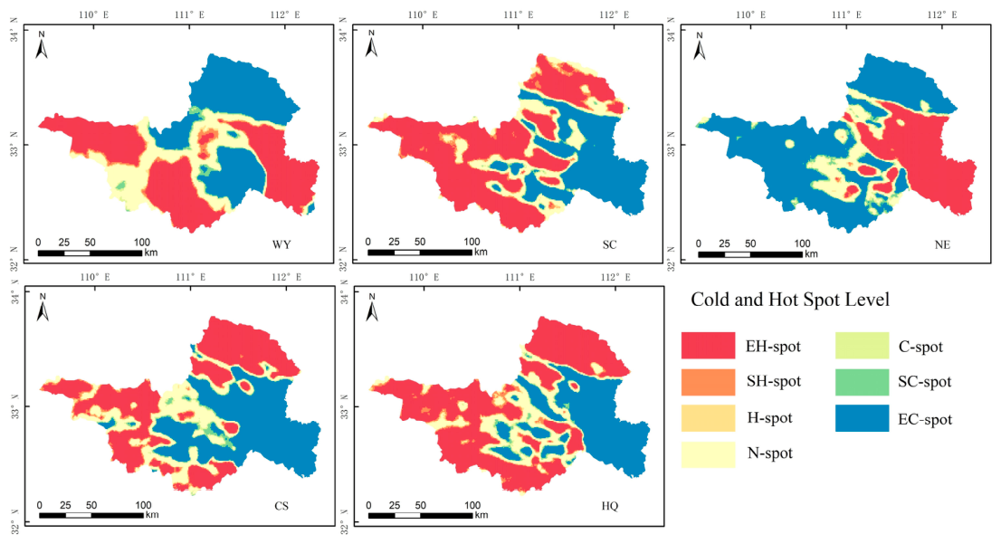
Using the 2020 ecosystem service distributions as analytical targets, hot–cold spot analysis was conducted to identify spatial clustering patterns (Figure 2). To support the map-based interpretation, hot–cold spot levels were summarized using hexagonal bins (

Table 4. Hexagon-based spatial statistics of hot–cold spot levels for ecosystem services.

Ecosystem Services	Mean	Median	Standard Deviation	Min	Max
Water Yield	0.20	0	2.58	−3.00	3.00
Soil Conservation	0.59	1.60	2.54	−3.00	3.00
Nitrogen Export	−0.86	−2.75	2.56	−3.00	3.00
Carbon Storage	0.06	0	2.57	−3.00	3.00
Habitat Quality	0.65	1.83	2.54	−3.00	3.00

and

Table 5. Chi-square test for hotspot hexagonal binning results.

Ecosystem Services	Cold Spots (−3 to −1), n (%)	Not Significant (0), n (%)	Hot Spots (1 to 3), n (%)	Total
Water Yield	755 (36.19%)	439 (21.05%)	892 (42.76%)	2086
Soil Conservation	642 (30.78%)	383 (18.36%)	1061 (50.86%)	2086
Nitrogen Export	1213 (58.15%)	286 (13.71%)	587 (28.14%)	2086
Carbon Storage	821 (39.36%)	409 (19.61%)	856 (41.04%)	2086
Habitat Quality	633 (30.35%)	355 (17.02%)	1098 (52.64%)	2086

Note: Cold spots combine classes −3 to −1, whereas hot spots combine classes 1 to 3. The chi-square test was conducted on the 5 × 3 contingency table: χ² = 497, df = 8, p < 0.001, Cramer’s V = 0.154.

). Water yield, soil conservation, carbon storage, and habitat quality were treated as positive indicators, for which hot spots indicate stronger ecosystem service supply. Nitrogen export was treated as a negative indicator, for which hot spots indicate higher nitrogen export pressure.

The hexagon-based results showed clear differences among ecosystem services. Soil conservation and habitat quality had positive mean hot–cold spot scores of 0.59 and 0.65, respectively, and their hot-spot proportions reached 50.86% and 52.64%, indicating stronger clustering of ecological service supply. Water yield and carbon storage showed weaker clustering tendencies, with mean scores close to zero and relatively balanced proportions of hot and cold spots. In contrast, nitrogen export showed a negative mean score of −0.86, with cold spots accounting for 58.15% of all bins, suggesting that low nitrogen export pressure dominated large parts of the study area.

The chi-square test showed that the distribution of cold spots, non-significant areas, and hot spots differed significantly among the five ecosystem services (χ² = 497, df = 8, p < 0.001), although the association strength was relatively weak (Cramer’s V = 0.154). Spatially, hot spots of soil conservation, carbon storage, and habitat quality were mainly concentrated in the northern and western mountainous areas, especially Xixia County and surrounding forested regions. In contrast, weaker ecological service supply and higher nitrogen export pressure were mainly observed in the eastern plains, including Dengzhou City and Neixiang County. Overall, the results indicate a clear mountain–plain differentiation in ecosystem service clustering.

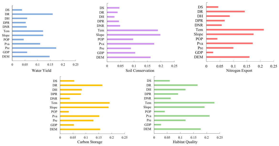
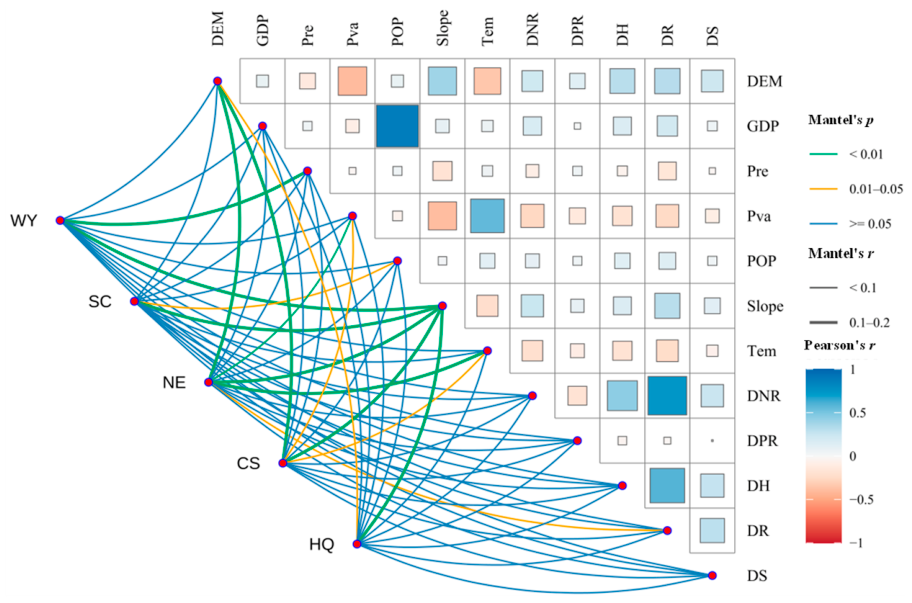
To further clarify spatial correlations between ecosystem services and driving factors, we conducted Mantel tests on five ecosystem services and 12 driving factors (Figure 3). Results showed that natural geographic factors—slope, DEM, annual temperature, annual precipitation, annual evapotranspiration—had significant or highly significant correlations with ecosystem services. Slope showed highly significant correlations with all five ecosystem services (p < 0.001), making it the most important driver of ecosystem service spatial distribution. DEM showed highly significant correlations with water yield, soil conservation, carbon storage, and habitat quality, but insignificant correlation with nitrogen export. Annual temperature showed highly significant correlations with water yield and nitrogen export. Annual precipitation showed highly significant correlations with water yield, soil conservation, and nitrogen export. Annual evapotranspiration showed highly significant correlations with water yield and nitrogen export. In contrast, socioeconomic factors—GDP, population density, distances to various transportation facilities—had relatively weak correlations with most ecosystem services, with only isolated factors showing significant correlations with individual services. For instance, GDP showed significant correlation with nitrogen export (p < 0.05), and distance to water systems showed significant correlation with habitat quality (p < 0.05). Overall, natural geographic factors dominated ecosystem service spatial patterns; socioeconomic factor influences remained relatively limited.

3.2.2. Factor Detection and Interaction Analysis

To further quantify the explanatory power of different driving factors for the spatial differentiation of ecosystem services, the optimal-parameter-based geographical detector was used for factor detection and interaction detection. Unlike the Mantel test, which focuses on spatial pattern correlations, the geographical detector uses the q value to measure the extent to which each factor explains the spatial heterogeneity of ecosystem services.

The factor detection results showed that climatic and topographic factors had relatively strong explanatory power for the spatial differentiation of ecosystem services (Figure 4). Annual mean temperature (Tem) showed strong explanatory power for nitrogen export (q = 0.213), carbon storage (q = 0.229), and habitat quality (q = 0.192). Slope was an important factor affecting soil conservation (q = 0.198) and carbon storage (q = 0.188). Precipitation (Pre) was the dominant explanatory factor for the spatial differentiation of water yield (q = 0.173). Compared with natural geographic factors, individual socioeconomic factors generally showed weaker explanatory power. However, some transportation accessibility variables, such as distance to railways (DR), still exhibited certain explanatory effects on water yield, nitrogen export, carbon storage, and habitat quality.

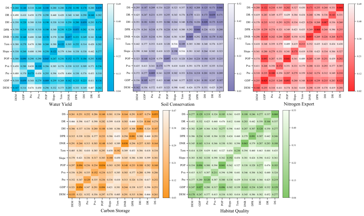
The interaction detection results showed that the explanatory power of any two-factor interaction was higher than that of individual factors, indicating that the spatial differentiation of ecosystem services was not controlled by a single factor, but was jointly shaped by natural geographic conditions, climatic conditions, and human activities (Figure 5). Among them, the interaction between population density (POP) and annual mean temperature (Tem) showed the highest explanatory power for nitrogen export (q = 0.489) and habitat quality (q = 0.527). This interaction may reflect the concentration of population, agricultural production, and construction land in the warmer eastern plains. Under these conditions, intensified human activities increase nutrient inputs and habitat disturbance, thereby simultaneously increasing nitrogen export pressure and reducing habitat quality. The interaction between elevation (DEM) and distance to railways (DR) showed strong explanatory power for water yield (q = 0.487) and carbon storage (q = 0.466). Elevation regulates precipitation, temperature, vegetation distribution, and hydrological processes, whereas distance to railways reflects differences in accessibility and human disturbance. Their combined effect therefore differentiates high-elevation, forest-dominated areas from more accessible agricultural and built-up areas, strengthening the spatial contrasts in water yield and carbon storage. The interaction between slope and annual mean temperature (Tem) had a strong explanatory effect on the spatial differentiation of soil conservation (q = 0.516). Steeper slopes increase erosion potential, while temperature affects vegetation growth and evapotranspiration. Their interaction indicates that the soil-conservation capacity of steep terrain depends partly on whether climatic conditions support sufficient vegetation cover. These results indicate that socioeconomic factors with relatively weak independent effects can exert substantially stronger influences when coupled with climatic or topographic conditions. Such interactions help explain the observed mountain–plain differentiation, with forested mountainous areas generally supporting soil conservation, carbon storage, and habitat quality, while the more intensively used eastern plains experience greater nitrogen export pressure. The synergies and trade-offs among ecosystem services themselves were further evaluated through the inter-service correlation analysis.

3.2.3. Spatial Trade-Off and Synergy Analysis

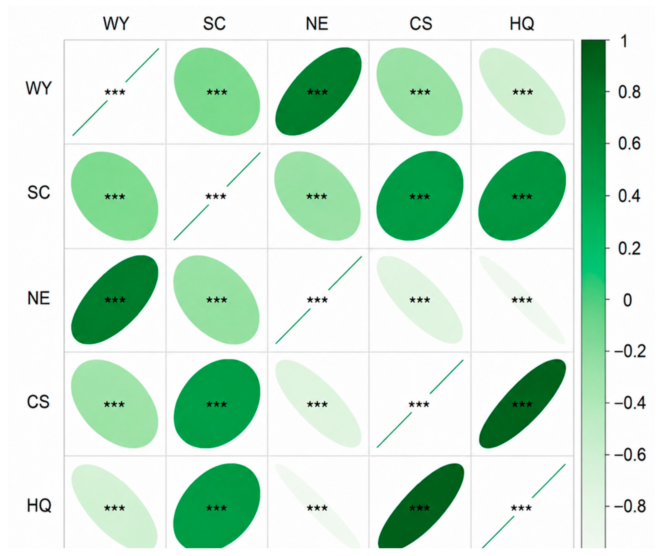
Pixel-wise Pearson correlation analysis revealed clear trade-offs and synergies among the five ecosystem services (Figure 6). Carbon storage (CS) and habitat quality (HQ) exhibited the strongest positive relationship, while soil conservation (SC) was also positively associated with both services. These correlations were consistent with the hot–cold spot patterns: the hot spots of SC, CS, and HQ largely overlapped in the northern, western, and southern forested mountains, whereas their cold spots were mainly distributed in the eastern plains. This spatial matching indicates a regulating–supporting service bundle jointly sustained by forest cover and vegetation conservation.

Nitrogen export (NE) was negatively correlated with SC, CS, and HQ. Spatially, NE hot spots were concentrated in the eastern agricultural and built-up plains, where these positive ecosystem services generally showed lower values. Conversely, NE cold spots largely coincided with the mountainous hot spots of SC, CS, and HQ. Because NE is a negative pressure indicator, these negative correlations should not be interpreted simply as ecological conflicts. Instead, they indicate that areas with stronger soil conservation, carbon storage, and habitat quality generally experience lower nutrient-export pressure, reflecting an ecological co-benefit between ecosystem protection and water-quality regulation.

Water yield (WY) showed a positive association with NE but negative relationships with SC, CS, and HQ. The coincidence of high WY and high NE in some eastern and central areas suggests that greater runoff production may enhance nutrient transport. Meanwhile, forested areas with high CS and HQ may produce relatively lower WY because of stronger canopy interception and evapotranspiration. These relationships reveal a potential spatial mismatch between water provision and regulating or supporting services.

The combined evidence from the correlation and hot–cold spot analyses revealed a distinct mountain–plain differentiation in ecosystem service bundles. Forested mountainous areas were characterized by matched high SC, CS, and HQ and low NE, whereas the eastern plains exhibited higher nutrient-export pressure and weaker regulating and supporting services. These spatial patterns identify mountainous forests as priority areas for maintaining multiple ecosystem services and eastern plains as key areas for nutrient control, habitat restoration, and coordinated land management.

3.3. Future Scenarios: Land-Use and Ecosystem Service Projections

3.3.1. Land-Use Change Under Climate Scenarios

The Taylor diagrams show that MRI-ESM2-0 provided the best overall representation of the observed meteorological conditions among the five GCMs and was therefore selected for subsequent scenario simulations (Figure S3). Based on the 2020 land-use data combined with future land-use datasets, land-use demands for 2050 were obtained under different SSP scenarios (

Table 6. Land-use types under different scenarios in 2050.

Land-Use Type	SSP126 (km2)	SSP245 (km2)	SSP585 (km2)
Cropland	6357.4	7265.5	7226.9
Forest	12,220.8	12,417.3	12,252.1
Grassland	2359	1685	1547
Water areas	844.2	740.7	611.9
Construction land	807.1	480.2	950.9
Unused land	1.9	1.5	1.4

). Under the modeled SSP assumptions, the simulated 2050 land-use structures showed different transition patterns relative to the 2020 baseline. Cropland remained a dominant land-use type and expanded under all scenarios, with increases of 2.19%, 16.78%, and 16.17% under SSP126, SSP245, and SSP585, respectively, indicating continued pressure on agricultural land demand. Forest area remained relatively stable, with only minor changes across scenarios, suggesting limited large-scale forest conversion. Grassland exhibited contrasting responses, remaining nearly stable under SSP126 but declining under SSP245 and SSP585, reflecting increasing conversion pressure under higher-intensity development pathways. Water areas decreased under all scenarios, with the greatest reduction under SSP585, indicating potential pressure on aquatic ecosystems under high-emission conditions. Construction land remained nearly stable under SSP126, decreased under SSP245, and increased under SSP585, indicating that future built-up land patterns were influenced by scenario-specific allocation assumptions rather than a uniform expansion trend. Unused land remained a minor land-use category with limited changes across scenarios.

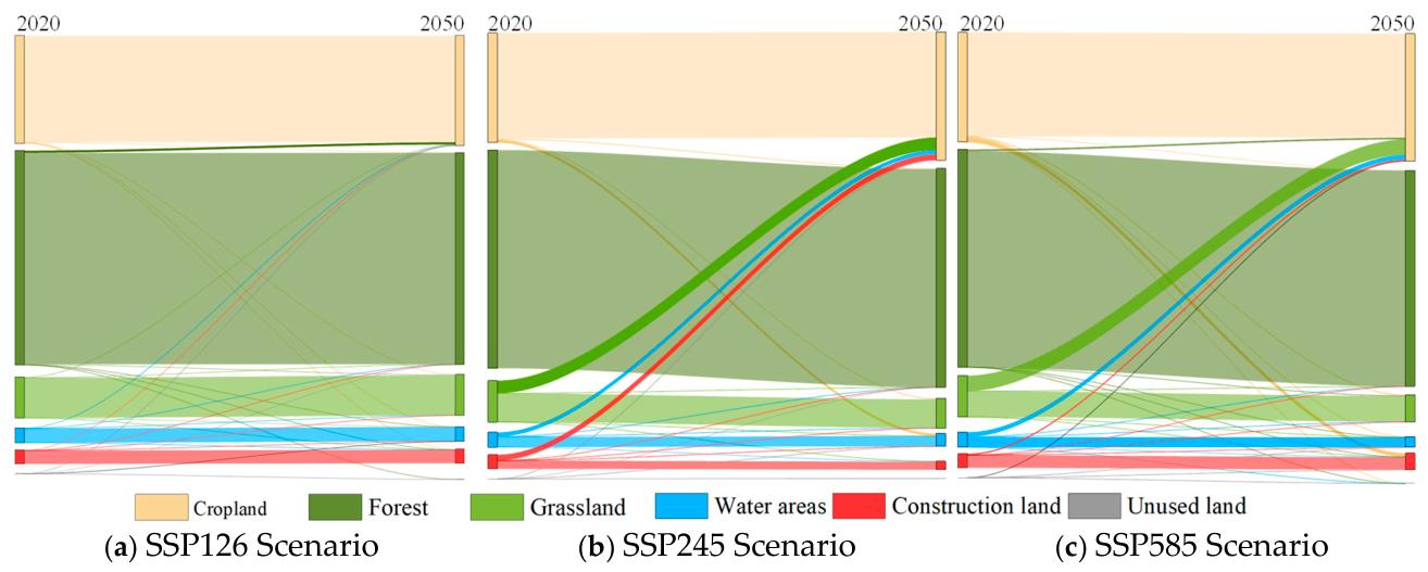
PLUS model simulations projected spatial distributions of land use in 2050 under SSP126, SSP245, and SSP585 scenarios (Figure S4). Compared with 2020, land-use type composition in 2050 did not undergo fundamental transformation under any scenario, remaining dominated by forest and cropland, though cropland expansion and grassland/water area reduction trends were pronounced. The magnitude and direction of land-use transitions varied among scenarios (

Table 7. Net changes in land-use types under different climate scenarios from 2020 to 2050.

Land-Use Type	SSP126 (km2)	SSP245 (km2)	SSP585 (km2)
Cropland	135.9	1044.1	1005.5
Forest	−137.8	58.8	−106.4
Grassland	5.1	−668.9	−806.9
Water areas	−8.4	−111.8	−240.7
Construction land	5	−321.9	148.9
Unused land	0.1	−0.3	−0.4

). SSP126 showed relatively limited land-use changes, characterized by modest cropland expansion and only minor changes in the other land-use types. In contrast, SSP245 and SSP585 exhibited stronger cropland expansion accompanied by grassland reduction, indicating increased pressure on natural ecosystems under higher-intensity development pathways. SSP585 showed the strongest grassland retreat and water-area reduction, reflecting stronger land-use transformation under high-emission conditions (Figure 7). Construction land showed different responses among scenarios, suggesting that future land-use patterns were influenced by scenario-specific allocation assumptions and spatial constraints rather than a uniform expansion trend.

3.3.2. Ecosystem Service Projections Under Climate Scenarios

Under the modeled SSP assumptions, the simulations indicated distinct ecosystem-service trajectories relative to the 2020 baseline (

Table 8. Quantitative projections of ecosystem services under future scenarios.

Scenario	Water Yield (mm)	Soil Conservation (×108 t)	Nitrogen Export (t)	Carbon Storage (×108 t)	Habitat Quality
2020	267.84	5.864	6823.978	2.146	0.578
2050-SSP126	321.86	5.855	6855.592	2.153	0.557
2050-SSP245	306.71	5.834	7571.409	2.182	0.546
2050-SSP585	117.13	5.827	7666.250	2.153	0.539

). Water yield increased under SSP126 and SSP245, rising from 267.84 mm to 321.86 mm and 306.71 mm, respectively, but decreased sharply to 117.13 mm under SSP585. Soil conservation changed only slightly across scenarios, while nitrogen export increased continuously, especially under SSP245 and SSP585. Carbon storage showed a slight increase, with the highest value under SSP245. In contrast, habitat quality declined under all future scenarios, decreasing from 0.578 in 2020 to 0.557, 0.546, and 0.539 under SSP126, SSP245, and SSP585, respectively. Under the modeled assumptions, SSP585 was associated with greater potential ecological pressures, reflected in lower water yield, higher nitrogen export, and lower habitat quality.

Compared with 2020, ecosystem services in 2050 showed clear scenario-dependent differences (Figure S5 and

Table 9. Hexagon-based spatial statistics of ecosystem services under future climate scenarios in 2050.

Ecosystem Services	Scenarios	Mean	Median	Standard Deviation	Min	Max
Water Yield	2020	271.64	256.32	90.30	0	662.31
	2050-SSP126	323.11	322.18	55.30	62.95	575.12
	2050-SSP245	307.60	300.43	63.43	59.99	605.05
	2050-SSP585	118.02	112.56	43.56	8.01	355.46
Soil Conservation	2020	255.72	294.57	129.27	2.75	531.61
	2050-SSP126	255.30	293.82	129.12	2.78	530.11
	2050-SSP245	254.39	294.08	129.64	2.17	530.11
	2050-SSP585	254.10	293.24	129.04	2.17	530.11
Nitrogen Export	2020	3.01	1.88	2.52	0	10.80
	2050-SSP126	3.03	1.93	2.50	0	10.80
	2050-SSP245	3.33	2.14	2.76	0	11.78
	2050-SSP585	3.37	2.30	2.68	0	11.78
Carbon Storage	2020	95.56	96.33	27.08	0	144.80
	2050-SSP126	95.63	105.00	23.47	0	119.46
	2050-SSP245	96.83	105.51	22.57	0	119.46
	2050-SSP585	95.58	105.21	23.75	0	119.46
Habitat Quality	2020	0.58	0.66	0.28	0.02	1.00
	2050-SSP126	0.56	0.67	0.25	0.02	1.00
	2050-SSP245	0.55	0.66	0.25	0.02	1.00
	2050-SSP585	0.54	0.65	0.25	0.02	1.00

). Water yield increased under SSP126 and SSP245, with the mean value rising from 271.64 mm in 2020 to 323.11 mm and 307.60 mm, respectively, but decreased sharply to 118.02 mm under SSP585. Soil conservation remained relatively stable across scenarios, although its mean value declined slightly from 255.72 t/ha in 2020 to 255.30, 254.39, and 254.10 t/ha under SSP126, SSP245, and SSP585, respectively. Nitrogen export increased under all scenarios, especially under SSP245 and SSP585, indicating intensified nitrogen export pressure in future development pathways.

Spatially, Figure S5 shows that high soil conservation, carbon storage, and habitat quality values remained mainly concentrated in mountainous and forested areas, while higher nitrogen export was still distributed in the eastern plain areas dominated by cropland and construction land. Overall, SSP126 and SSP245 were more favorable for maintaining ecosystem services, whereas the SSP585 simulation indicated substantially lower water yield, higher nitrogen export pressure, and greater potential ecological pressure.

4. Discussion

4.1. Mechanisms Driving Ecosystem Service Differentiation

The spatial differentiation of ecosystem services was jointly controlled by topography, climate, vegetation, and human activity, but the relative role of each factor differed by service. Slope was the only factor with highly significant Mantel correlations with all five services (p < 0.001), which indicates that it operated not as a single mechanism but as a compound gradient that simultaneously encoded erosion dynamics, vertical vegetation zonation, and human accessibility. Steep, forested mountain slopes combined high erosion potential, dense vegetation cover, and limited accessibility, jointly sustaining soil conservation, carbon storage, and habitat quality [39,40,41]; the same gradient limited the build-up of nutrient pressure, which explains why nitrogen export showed no significant Mantel correlation with elevation. Previous studies have similarly shown that ecosystem-service patterns and trade-offs are jointly shaped by climate–land cover interactions and multiple environmental drivers [42,43]. Climate factors acted service-specifically rather than uniformly. Annual temperature explained much of the spatial variation in nitrogen export (q = 0.213), carbon storage (q = 0.229), and habitat quality (q = 0.192) by regulating vegetation growth and nutrient cycling, whereas precipitation was the dominant single factor for water yield (q = 0.173), consistent with water-balance control of runoff generation [44,45].

The most informative result came from interaction detection, which showed that every two-factor interaction exceeded its individual factors. The population density–temperature interaction reached the highest explanatory power for both nitrogen export (q = 0.489) and habitat quality (q = 0.527). This is best interpreted as a climate-amplification mechanism: human disturbance (population concentration, agricultural intensity, and built-up expansion) is not translated into ecological pressure linearly but is amplified where warmer conditions accelerate nutrient cycling and extend the growing season, concentrating pressure in the warmer eastern plains [41]. Similarly, the slope–temperature interaction (q = 0.516) for soil conservation indicates that the protective capacity of steep terrain depends on whether climate supports sufficient vegetation cover, a mechanism that decouples apparent terrain sensitivity from actual erosion risk. Socioeconomic factors with weak independent effects (e.g., population density and accessibility) therefore exerted substantial influence only when coupled with climatic or topographic conditions, consistent with the view that human pressures in such source areas are expressed through their coupling with environmental gradients rather than in isolation.

4.2. Trade-Offs and Synergies Among Ecosystem Services

The correlation analysis revealed two spatially separated service bundles that define the region’s core management problem. Forested mountains formed a regulating–supporting bundle in which soil conservation, carbon storage, and habitat quality were strongly and positively associated: their hot spots largely overlapped in the northern, western, and southern mountains, and their cold spots coincided in the eastern plains (χ² = 497, p < 0.001). Nitrogen export was negatively correlated with these three services, but this should be read as an ecological co-benefit rather than a service conflict: areas with strong soil conservation, carbon storage, and habitat quality simultaneously experience lower nutrient-export pressure, so protecting the forest bundle and protecting water quality are the same action [36,43].

Water yield broke this pattern. It was positively associated with nitrogen export and negatively associated with soil conservation, carbon storage, and habitat quality: high-runoff areas in the east and center coincided with high nutrient export, while high-carbon forest areas produced relatively lower runoff owing to canopy interception and evapotranspiration. This reveals a genuine water-provision versus regulation-supply trade-off embedded in the mountain–plain structure, and it is precisely this trade-off that gives the study area its dual consequence. A management strategy that maximizes water yield for downstream delivery, for example by converting forest to low-vegetation land, would simultaneously raise nitrogen export and reduce local carbon storage and habitat quality, trading downstream water quantity against upstream water quality and ecological integrity. Because the water source area must sustain both local ecosystem functions and downstream supply security [10,26], the trade-off cannot be resolved by maximizing any single service; it must be managed as a bundle-level allocation problem, with forests as the joint guarantee of water quality and local services and plains as the target of nutrient control.

4.3. Ecosystem Service Responses Under Alternative SSP Scenarios

Under the modeled assumptions, the three SSPs produced divergent trajectories that illustrate both the sensitivity and the limits of scenario-based projection. Water yield increased by 20.1% under SSP126 (321.86 mm) and 14.5% under SSP245 (306.71 mm) relative to the 2020 baseline (267.84 mm) but fell by 56.3% under SSP585 (117.13 mm). The magnitude of the SSP585 decline deserves scrutiny: it arises from the combined effect of stronger warming (raising evapotranspiration demand) and intensified land-use pressure, consistent with studies showing that climate and land-use changes jointly govern water yield and that their relative contributions vary across watersheds [44,45]. Because this projection rests on a single selected GCM (MRI-ESM2-0) and on the allocation rules embedded in the future land-use dataset, the extreme SSP585 result should be treated as an upper-bound pressure signal rather than a quantitative forecast; a multi-model ensemble would narrow the confidence interval around this estimate.

Two results were counterintuitive and require explicit interpretation. First, carbon storage increased slightly in all future scenarios despite having declined by 3.23% historically (98.75 to 95.56 t/ha). This reversal reflects a model assumption, that forest area remains stable under the projected land-use demands, rather than an observed ecological recovery. The historical decline shows that even limited forest and grassland losses (74.41 km² and 21.25 km² of reduction during 2005–2020) were sufficient to reduce carbon pools, because biomass and soil carbon recover slowly after disturbance. The scenario-based stability therefore likely underestimates future carbon-loss risk whenever land conversion exceeds the modeled allocation, and carbon storage should not be treated as secure under any pathway. Second, nitrogen export increased under all scenarios, driven mainly by continued cropland expansion (16.78% and 16.17% increases in cropland under SSP245 and SSP585), and even where construction land decreased (SSP245), cropland-driven nutrient pressure persisted. This confirms that nutrient export is governed more by agricultural extent and hydrological connectivity than by built-up area, and it implies that land-use-based nutrient control must target the agricultural land base itself rather than urbanization [42].

Habitat quality declined monotonically from 0.578 in 2020 to 0.557, 0.546, and 0.539 under SSP126, SSP245, and SSP585, respectively. Because forest area remained stable in all scenarios, this decline was driven by habitat degradation and fragmentation processes embedded in the land-use projections rather than by deforestation per se, a reminder that habitat quality can deteriorate even where gross forest cover is maintained and that monitoring must track landscape configuration, not just area [42,43]. Overall, SSP126 and SSP245 better preserved water source functions, whereas SSP585 was associated with lower water yield, higher nitrogen export, and lower habitat quality, consistent with evidence that high-emission pathways generally intensify pressure on water regulation, nutrient regulation, and habitat quality across climate-sensitive watersheds, although the magnitude varies with regional climate, vegetation, and land-use intensity [42,45].

4.4. Management Implications for Water Source Areas

The mountain–plain bundle structure translates directly into a differentiated management strategy. The northern, western, and southern forested mountains (e.g., the Funiu Mountains in Xixia County) function as the region’s multifunctional ecological barrier, simultaneously supplying soil conservation, carbon storage, habitat quality, and water-quality regulation; they should remain priority conservation zones under a strict forest-protection regime, with conversion restrictions and vegetation restoration on degraded patches [23,26,40]. The eastern agricultural plains (e.g., Dengzhou and Neixiang) are the nitrogen-control zone, where management should target the agricultural land base through precision fertilization, riparian buffer strips, and nutrient-reduction or fallow programs rather than construction land, since nutrient export proved insensitive to built-up area [36,43].

Because the water source area faces the dual consequence of sustaining local functions and guaranteeing downstream supply, the linkage between the two should also be institutionalized. The scenario results suggest that conservation and supply objectives align under sustainable pathways but diverge under SSP585, so adaptive planning is required: under high-emission trajectories, the risk of a simultaneous decline in water yield and rise in nutrient pressure would propagate downstream, and ecological compensation and counterpart-cooperation mechanisms between the source area and beneficiary regions should be tied to verifiable service outcomes rather than to inputs. We propose nitrogen export and carbon storage as the two core monitoring indicators, since they capture the region’s principal pressures and respond to both land-use and climate signals. Finally, service trade-offs should be managed explicitly at the bundle level: where water provision and regulating services conflict, decision-makers should evaluate the joint consequences for downstream quantity and quality instead of optimizing water yield alone [10,24,26].

4.5. Limitations and Future Research Directions

Several uncertainties qualify these findings. First, InVEST parameters were largely drawn from published studies in the region and comparable areas because site-specific measurements were unavailable; without field calibration, formal parameter sensitivity analysis and uncertainty quantification were not possible. Future work should couple field observations with Monte Carlo approaches to bound parameter-induced uncertainty. Second, future projections inherit the assumptions of the land-use dataset, the SSP narratives, and the climate simulations. The scenario-dependent construction-land trajectories (stable under SSP126, declining under SSP245, increasing under SSP585) reflect the allocation rules embedded in the dataset rather than region-specific policy effects, and region-specific socioeconomic scenarios with policy-based counterfactual simulations would improve realism. Third, although five CMIP6 GCMs were evaluated, only MRI-ESM2-0 was retained for projection; multi-model ensembles would better characterize climate uncertainty, particularly for the extreme water-yield response under SSP585. Fourth, the trade-off and synergy analysis is correlation-based and does not establish causality; spatial panel or process-based approaches would be needed to distinguish causal service relationships from shared drivers. Extending this framework with these improvements, and applying it to other inter-basin water transfer source areas, would test the generalizability of the mountain–plain bundle structure and the pathway-dependent pressures identified here.

5. Conclusions

This study coupled historical ecosystem service assessment with spatial statistics, driver attribution, and SSP-based scenario simulation to answer three questions about the core water source area of the Middle Route of the South-to-North Water Diversion Project.

First, on spatiotemporal patterns, ecosystem services were broadly stable in aggregate between 2005 and 2020, but this stability masked divergent trends: water yield changed marginally (+0.34%), soil conservation remained essentially unchanged, nitrogen export rose from 6774.30 t to 6823.98 t, and carbon storage declined by 3.23% (98.75 to 95.56 t/ha) while habitat quality slipped from 0.580 to 0.578. The region thus entered this period with emerging nutrient pressure and carbon loss even as headline functions appeared stable.

Second, on driving mechanisms, spatial differentiation was dominated by natural factors, with slope the only factor significantly correlated with all five services (p < 0.001) as a compound topographic gradient and climate factors acting service-specifically. The decisive finding was that interactions systematically exceeded individual factors: the population density–temperature interaction was strongest for nitrogen export (q = 0.489) and habitat quality (q = 0.527), and the slope–temperature interaction was strongest for soil conservation (q = 0.516). Human pressures therefore operated through coupling with climatic and topographic conditions rather than independently.

Third, on future trajectories, water yield by 2050 increased under SSP126 (+20.1%, 321.86 mm) and SSP245 (+14.5%, 306.71 mm) but fell sharply under SSP585 (−56.3%, 117.13 mm); nitrogen export increased under all scenarios, carbon storage rose slightly as a modeling artifact of assumed stable forest area, and habitat quality declined monotonically to 0.557, 0.546, and 0.539 under SSP126, SSP245, and SSP585. SSP126 and SSP245 better supported the maintenance of water source functions, whereas SSP585 implied greater potential pressures reflected in lower water yield, higher nitrogen export, and lower habitat quality.

References

1. Millennium Ecosystem Assessment. Ecosystems and Human Well-Being: Synthesis; Island Press: Washington, DC, USA, 2005. [Google Scholar]
2. Costanza, R.; De Groot, R.; Sutton, P.; van der Ploeg, S.; Anderson, S.J.; Kubiszewski, I.; Farber, S.; Turner, R.K. Changes in the global value of ecosystem services. Glob. Environ. Change 2014, 26, 152–158. [Google Scholar] [CrossRef] [Scilit]
3. Díaz, S.; Settele, J.; Brondízio, E.S.; Ngo, H.T.; Agard, J.; Arneth, A.; Balvanera, P.; Brauman, K.A.; Butchart, S.H.M.; Chan, K.M.A.; et al. Pervasive human-driven decline of life on Earth points to the need for transformative change. Science 2019, 366, eaax3100. [Google Scholar] [CrossRef] [Scilit] [PubMed]
4. Foley, J.A.; DeFries, R.; Asner, G.P.; Barford, C.; Bonan, G.; Carpenter, S.R.; Chapin, F.S.; Coe, M.T.; Daily, G.C.; Gibbs, H.K.; et al. Global consequences of land use. Science 2005, 309, 570–574. [Google Scholar] [CrossRef] [Scilit] [PubMed]
5. Ouyang, Z.; Zheng, H.; Xiao, Y.; Polasky, S.; Liu, J.; Xu, W.; Wang, Q.; Zhang, L.; Xiao, Y.; Rao, E.; et al. Improvements in ecosystem services from investments in natural capital. Science 2016, 352, 1455–1459. [Google Scholar] [CrossRef] [Scilit] [PubMed]
6. Song, X.P.; Hansen, M.C.; Stehman, S.V.; Potapov, P.V.; Tyukavina, A.; Vermote, E.F.; Townshend, J.R. Global land change from 1982 to 2016. Nature 2018, 560, 639–643. [Google Scholar] [CrossRef] [Scilit] [PubMed]
7. Seto, K.C.; Güneralp, B.; Hutyra, L.R. Global forecasts of urban expansion to 2030 and direct impacts on biodiversity and carbon pools. Proc. Natl. Acad. Sci. USA 2012, 109, 16083–16088. [Google Scholar] [CrossRef] [Scilit] [PubMed]
8. Kong, W.; Shen, W.; Yu, C.; Niu, L.; Zhou, H.; Zhang, Z.; Guo, S. The neglected cost: Ecosystem services loss due to urban expansion in China from a triple-coupling perspective. Environ. Impact Assess. Rev. 2025, 112, 107827. [Google Scholar] [CrossRef] [Scilit]
9. IPBES. Summary for Policymakers of the Global Assessment Report on Biodiversity and Ecosystem Services; IPBES Secretariat: Bonn, Germany, 2019. [Google Scholar]
10. Zhuang, N.; Wang, M.; Shi, C.; Fu, S.; Yang, Q.; Ding, C.; Ouyang, Y.; Liu, H. Assessing the impacts of inter-basin water transfer projects on ecosystem services in water source areas: Evidence from the Hanjiang River Basin. PLoS ONE 2025, 20, e0323068. [Google Scholar] [CrossRef] [Scilit] [PubMed]
11. Xie, G.D.; Zhang, C.X.; Zhang, L.M.; Chen, W.H.; Li, S.M. Improvement of the evaluation method for ecosystem service value based on per unit area value equivalent factor. J. Nat. Resour. 2015, 30, 1243–1254. [Google Scholar] [CrossRef]
12. Nelson, E.; Mendoza, G.; Regetz, J.; Polasky, S.; Tallis, H.; Cameron, D.R.; Chan, K.M.A.; Daily, G.C.; Goldstein, J.; Kareiva, P.M.; et al. Modeling multiple ecosystem services, biodiversity conservation, commodity production, and tradeoffs at landscape scales. Front. Ecol. Environ. 2009, 7, 4–11. [Google Scholar] [CrossRef] [Scilit]
13. Liu, W.; Zhan, J.; Zhao, F.; Wang, C.; Zhang, F.; Teng, Y.; Chu, X.; Kumi, M.A. Spatio-temporal variations of ecosystem services and their drivers in the Pearl River Delta, China. J. Clean. Prod. 2022, 337, 130466. [Google Scholar] [CrossRef] [Scilit]
14. Shao, Y.; Liu, Y.; Li, Y.; Yuan, X. Regional ecosystem services relationships and their potential driving factors in the Yellow River Basin, China. J. Geogr. Sci. 2023, 33, 863–884. [Google Scholar] [CrossRef] [Scilit]
15. Li, Y.; Luo, H. Trade-off/synergistic changes in ecosystem services and geographical detection of its driving factors in typical karst areas in southern China. Ecol. Indic. 2023, 154, 110811. [Google Scholar] [CrossRef] [Scilit]
16. Liu, X.; Liang, X.; Li, X.; Xu, X.; Ou, J.; Chen, Y.; Li, S.; Wang, S.; Pei, F. A future land use simulation model (FLUS) for simulating multiple land use scenarios by coupling human and natural effects. Landsc. Urban Plan. 2017, 168, 94–116. [Google Scholar] [CrossRef] [Scilit]
17. Fu, F.; Deng, S.; Wu, D.; Liu, W.; Bai, Z. Research on the spatiotemporal evolution of land use landscape pattern in a county area based on CA-Markov model. Sustain. Cities Soc. 2022, 80, 103760. [Google Scholar] [CrossRef] [Scilit]
18. Verburg, P.H.; Soepboer, W.; Veldkamp, A.; Limpiada, R.; Espaldon, V.; Mastura, S.S.A. Modeling the spatial dynamics of regional land use: The CLUE-S model. Environ. Manag. 2002, 30, 391–405. [Google Scholar] [CrossRef] [Scilit] [PubMed]
19. Liang, X.; Guan, Q.; Clarke, K.C.; Liu, S.; Wang, B.; Yao, Y. Understanding the drivers of sustainable land expansion using a patch-generating land use simulation (PLUS) model: A case study in Wuhan, China. Comput. Environ. Urban Syst. 2021, 85, 101569. [Google Scholar] [CrossRef] [Scilit]
20. Li, Z.; Jiang, W.; Peng, K.; Wang, X.; Deng, Y.; Yin, X.; Ling, Z. Comparative analysis of land use change prediction models for land and fine wetland types: Taking the wetland cities Changshu and Haikou as examples. Landsc. Urban Plan. 2024, 243, 104975. [Google Scholar] [CrossRef] [Scilit]
21. Riahi, K.; van Vuuren, D.P.; Kriegler, E.; Edmonds, J.; O’Neill, B.C.; Fujimori, S.; Bauer, N.; Calvin, K.; Dellink, R.; Fricko, O.; et al. The Shared Socioeconomic Pathways and their energy, land use, and greenhouse gas emissions implications: An overview. Glob. Environ. Change 2017, 42, 153–168. [Google Scholar] [CrossRef] [Scilit]
22. Meinshausen, M.; Nicholls, Z.R.J.; Lewis, J.; Gidden, M.J.; Vogel, E.; Freund, M.; Beyerle, U.; Gessner, C.; Nauels, A.; Bauer, N.; et al. The Shared Socio-Economic Pathway greenhouse gas concentrations and their extensions to 2500. Geosci. Model Dev. 2020, 13, 3571–3605. [Google Scholar] [CrossRef] [Scilit]
23. Liu, L.; Zheng, L.; Wang, Y.; Liu, C.; Zhang, B.; Bi, Y. Land Use and Ecosystem Services Evolution in Danjiangkou Reservoir Area, China: Implications for Sustainable Management of National Projects. Land 2023, 12, 788. [Google Scholar] [CrossRef] [Scilit]
24. Zhang, J.; Guo, W.; Wang, Y.; Tang, Z.; Qi, L. Identifying the regional spatial management of ecosystem services from a supply and demand perspective: A case study of Danjiangkou reservoir area, China. Ecol. Indic. 2024, 158, 111421. [Google Scholar] [CrossRef] [Scilit]
25. Zhuang, W. Eco-environmental impact of inter-basin water transfer projects: A review. Environ. Sci. Pollut. Res. 2016, 23, 12867–12879. [Google Scholar] [CrossRef] [Scilit] [PubMed]
26. Zhao, P.; Wang, L.; Huang, Y.; Zhao, Y.; Yang, Q.; Huang, J.; Du, Y.; Ling, F. Comprehensive evaluation and scenario simulation for determining the optimal conservation priority of ecological services in Danjiangkou Reservoir Area, China. Ecol. Indic. 2024, 169, 112906. [Google Scholar] [CrossRef] [Scilit]
27. O’Neill, B.C.; Tebaldi, C.; van Vuuren, D.P.; Eyring, V.; Friedlingstein, P.; Hurtt, G.; Knutti, R.; Kriegler, E.; Lamarque, J.-F.; Lowe, J.; et al. The Scenario Model Intercomparison Project (ScenarioMIP) for CMIP6. Geosci. Model Dev. 2016, 9, 3461–3482. [Google Scholar] [CrossRef] [Scilit]
28. Mutale, B.; Qiang, F. Modeling future land use and land cover under different scenarios using patch-generating land use simulation model. A case study of Ndola district. Front. Environ. Sci. 2024, 12, 1362666. [Google Scholar] [CrossRef] [Scilit]
29. Zarandian, A.; Mohammadyari, F.; Mirsanjari, M.M.; Visockiene, J.S. Scenario modeling to predict changes in land use/cover using Land Change Modeler and InVEST model: A case study of Karaj Metropolis, Iran. Environ. Monit. Assess. 2023, 195, 273. [Google Scholar] [CrossRef] [Scilit] [PubMed]
30. Zhang, J.; Lai, X.; Long, A.; Zhang, P.; Deng, X.; Deng, M.; Ren, C.; Xiao, Y. Water-ecological health assessment considering water supply-demand balance and water supply security: A case study in Xinjiang. Remote Sens. 2024, 16, 3834. [Google Scholar] [CrossRef] [Scilit]
31. Renard, K.G.; Foster, G.R.; Weesies, G.A.; McCool, D.K.; Yoder, D.C. Predicting Soil Erosion by Water: A Guide to Conservation Planning with the Revised Universal Soil Loss Equation (RUSLE); Agriculture Handbook No. 703; U.S. Department of Agriculture: Washington, DC, USA, 1997; 404p.
32. Duolaiti, X.; Kasimu, A.; Reheman, R.; Aizizi, Y.; Wei, B. Assessment of water yield and water purification services in the arid zone of Northwest China: The case of the Ebinur Lake Basin. Land 2023, 12, 533. [Google Scholar] [CrossRef] [Scilit]
33. Sharma, R.; Pradhan, L.; Kumari, M.; Bhattacharya, P.; Mishra, V.N.; Kumar, D. Spatio-temporal assessment of urban carbon storage and its dynamics using InVEST model. Land 2024, 13, 1387. [Google Scholar] [CrossRef] [Scilit]
34. Rahimi, L.; Malekmohammadi, B.; Yavari, A.R. Assessing and modeling the impacts of wetland land cover changes on water provision and habitat quality ecosystem services. Nat. Resour. Res. 2020, 29, 3701–3718. [Google Scholar] [CrossRef] [Scilit]
35. Duan, Y.M.; Fu, J.B.; Zhou, Y. Evolution characteristics of the “production-living-ecological” space and ecological effects in the water source area of the Middle Route of the South-to-North Water Diversion Project. China Popul. Resour. Environ. 2024, 34, 138–150. [Google Scholar]
36. Zhang, J.; Guo, W.; Cheng, C.; Tang, Z.; Qi, L. Trade-offs and driving factors of multiple ecosystem services and bundles under spatiotemporal changes in the Danjiangkou Basin, China. Ecol. Indic. 2022, 144, 109550. [Google Scholar] [CrossRef] [Scilit]
37. Wei, B.; Kasimu, A.; Fang, C.; Reheman, R.; Zhang, X.; Han, F.; Zhao, Y.; Aizizi, Y. Establishing and optimizing the ecological security pattern of the urban agglomeration in arid regions of China. J. Clean. Prod. 2023, 427, 139301. [Google Scholar] [CrossRef] [Scilit]
38. Song, Y.; Wang, J.; Ge, Y.; Xu, C. An optimal parameters-based geographical detector model enhances geographic characteristics of explanatory variables for spatial heterogeneity analysis: Cases with different types of spatial data. GISci. Remote Sens. 2020, 57, 593–610. [Google Scholar] [CrossRef] [Scilit]
39. Guo, S.; Huang, J.; Zhang, X.; Zhu, G.; Wen, Y. LUCC-based analysis of ecosystem service value drivers in the South–North Water Transfer Central Line recharge area. Environ. Earth Sci. 2023, 82, 289. [Google Scholar] [CrossRef] [Scilit]
40. Qi, W.; Li, H.; Zhang, Q.; Zhang, K. Forest restoration efforts drive changes in land-use/land-cover and water-related ecosystem services in China’s Han River Basin. Ecol. Eng. 2019, 126, 64–73. [Google Scholar] [CrossRef] [Scilit]
41. Han, R.; Feng, C.-C.; Xu, N.; Guo, L. Spatial heterogeneous relationship between ecosystem services and human disturbances: A case study in Chuandong, China. Sci. Total Environ. 2020, 721, 137818. [Google Scholar] [CrossRef] [Scilit] [PubMed]
42. Yu, Y.; Gao, S.; Wang, J.; Cheng, Q.; Deng, H.; Shen, Y. Unraveling climate–land cover interactions: How SSP–RCP scenarios drive ecosystem service trade-offs in contrasting Yangtze and Yellow River Basins, China. Landsc. Ecol. 2026, 41, 34. [Google Scholar] [CrossRef] [Scilit]
43. Wang, G.; Yue, D.; Niu, T.; Yu, Q. Regulated Ecosystem Services Trade-Offs: Synergy Research and Driver Identification in the Vegetation Restoration Area of the Middle Stream of the Yellow River. Remote Sens. 2022, 14, 718. [Google Scholar] [CrossRef] [Scilit]
44. Zhu, K.; Cheng, Y.; Zhou, Q.; Kápolnai, Z. The contributions of climate and land use/cover changes to water yield services considering geographic scale. Heliyon 2023, 9, e20115. [Google Scholar] [CrossRef] [Scilit] [PubMed]
45. Guo, Q.; Yu, C.; Xu, Z.; Yang, Y.; Wang, X. Impacts of climate and land-use changes on water yields: Similarities and differences among typical watersheds distributed throughout China. J. Hydrol. Reg. Stud. 2023, 45, 101294. [Google Scholar] [CrossRef] [Scilit]
Figure 1. Geographic location of the study area.
Land 15 01473 g001
Figure 2. Spatial distribution of ecosystem service hot and cold spots.
Land 15 01473 g002
Figure 3. Mantel test results for ecosystem services and driving factors. Note: WY, water yield; SC, soil conservation; NE, nitrogen export; CS, carbon storage; HQ, habitat quality; DEM, elevation derived from the digital elevation model; GDP, gross domestic product; Pre, annual precipitation; Pva, annual evapotranspiration; POP, population density; Slope, terrain slope; Tem, annual mean temperature; DNR, distance to national roads; DPR, distance to provincial roads; DH, distance to highways; DR, distance to railways; and DS, distance to water systems.
Land 15 01473 g003
Figure 4. Factor detection results for driving factors. Note: DEM, elevation derived from the digital elevation model; GDP, gross domestic product; Pre, annual precipitation; Pva, annual evapotranspiration; POP, population density; Slope, terrain slope; Tem, annual mean temperature; DNR, distance to national roads; DPR, distance to provincial roads; DH, distance to highways; DR, distance to railways; and DS, distance to water systems.
Land 15 01473 g004
Figure 5. Factor interaction detection results. Note: DEM, elevation derived from the digital elevation model; GDP, gross domestic product; Pre, annual precipitation; Pva, annual evapotranspiration; POP, population density; Slope, terrain slope; Tem, annual mean temperature; DNR, distance to national roads; DPR, distance to provincial roads; DH, distance to highways; DR, distance to railways; and DS, distance to water systems.
Land 15 01473 g005
Figure 6. Correlation analysis among ecosystem services. Note: Ellipse orientation indicates the direction of correlation, while ellipse narrowness and color intensity represent correlation strength. Narrower ellipses indicate stronger correlations. *** indicates p < 0.001. WY, water yield; SC, soil conservation; NE, nitrogen export; CS, carbon storage; HQ, habitat quality.
Land 15 01473 g006
Figure 7. Sankey diagrams of land-use transitions from 2020 to 2050 under future climate scenarios.
Land 15 01473 g007