


Abstract
Cropland non-grain use has become an important challenge for food security and cropland governance in rapidly urbanising agricultural regions, yet its trajectory heterogeneity and the divergence between current spatial patterns and long-term-change mechanisms remain insufficiently understood. Taking the Changsha–Zhuzhou–Xiangtan (CZT) urban agglomeration in China as a case, this study quantified the cropland non-grain rate (NGR) on a 1 km grid for 2000, 2010, and 2020, classified grid-level transition trajectories, and developed three temporally structured eXtreme Gradient Boosting (XGBoost) models with spatial block cross-validation, Shapley additive explanations (SHAP) interpretation, and geographically explicit SHAP (GeoSHAP) local attribution. The results show that low-NGR and stable grids formed the dominant regional background, while recent NGR increases were mainly concentrated along the urban development corridor and metropolitan fringe. Current NGR status and long-term NGR change showed divergent explanatory structures. The current spatial pattern was mainly associated with terrain constraints and contemporary urban pressure, whereas long-term change was more strongly conditioned by baseline urbanisation and subsequent urban–environmental changes. Nonlinear dependence analysis further identified model-derived response zones related to slope, impervious surface conditions, hydrothermal change, and hydrological proximity. GeoSHAP mapping revealed that locally dominant mechanisms varied substantially across the study area, indicating that cropland non-grain use was shaped by spatially heterogeneous combinations of terrain, urbanisation, hydrothermal background, and hydrological context. These findings support a shift from aggregate status monitoring toward trajectory-specific and mechanism-differentiated cropland management in urban agglomerations.
1. Introduction
Cropland non-grain use, commonly discussed in China as non-grain production on cultivated land, has become a growing concern for national food security and cropland governance under rapid urbanisation, rural labour restructuring, and shifting comparative agricultural returns [1,2,3]. Unlike the direct conversion of cropland to non-agricultural uses, non-grain use reflects a shift in land-use orientation and productive function within existing cultivated land, manifested through crop-structure substitution, the expansion of economic crops, aquaculture, nursery stock, or cash-crop plantation at the expense of major-grain production [4,5]. Because this process is often gradual, cumulative, and partly concealed within reported cropland area statistics, it can weaken regional grain-production capacity without triggering formal land-conversion controls, making it an increasingly important but analytically elusive challenge for cultivated land governance [6]. In urban agglomerations, where construction expansion, factor agglomeration, and land marketisation reshape land-rent gradients and intensify spatial differentiation, the cropland non-grain rate (NGR) is likely to be spatially heterogeneous and locally differentiated, demanding spatially explicit analysis rather than aggregate regional characterisation [7,8].
Most existing studies on cropland non-grain use have characterised its spatial extent and associated drivers using cross-sectional data at a single time point or through aggregate administrative-unit comparisons [2,9]. While this body of work has established important baselines—documenting that peri-urban proximity, terrain constraints, off-farm income opportunities, and land marketisation are consistently associated with elevated NGR levels [4,10]—cross-sectional approaches are fundamentally unable to distinguish trajectories of change from states of persistence. Two grids with identical current NGR values may have arrived there through sustained intensification, recent reversal, or long-term stability, each carrying different implications for management. Moreover, broad spatial averages tend to smooth out the heterogeneous trajectory structure of cropland systems, masking localised intensification corridors, areas of partial recovery, and zones of bidirectional fluctuation [11,12]. The limited attention to trajectory-level characterisation therefore leaves a critical gap in understanding the process heterogeneity underlying observed NGR spatial patterns and governing their future evolution.
A second and closely related gap concerns the mechanisms that shape non-grain use and its change. Even when temporal change is examined, most studies apply the same predictors to both current NGR levels and change magnitudes without explicitly asking whether the two analytical targets are governed by the same explanatory structure [9,10]. Current NGR patterns and long-term changes in NGR (ΔNGR) may respond to different combinations of contemporary conditions, historical contexts, and change processes, and conflating these two targets risks misidentifying intervention priorities or producing mechanism inferences that are sensitive to the temporal scope of the analysis [13,14]. Separating the drivers of spatial patterns from those of long-term NGR changes, and evaluating pre-existing conditions alongside concurrent changes, is therefore important for both interpretation and governance.
Identifying spatially heterogeneous, nonlinear mechanisms across these two analytical targets also presents methodological challenges. NGR processes are shaped by terrain constraints, urban pressure, climate background, and accessibility gradients that interact in complex, locally variable ways rather than through uniform linear relationships [12,15]. Nonlinear response transitions—where small changes in terrain gradient, urbanisation intensity, or hydrothermal conditions produce disproportionate shifts in NGR—are analytically important because they help distinguish stable zones from transition-sensitive areas and can inform spatially differentiated management [16,17]. Where high dimensionality, spatial autocorrelation, and nonlinearity coexist, conventional regression frameworks that assume global parameter stability or additive variable effects are often insufficient for identifying response transitions and spatially differentiated mechanism structures [18,19].
Tree-based machine learning approaches, particularly eXtreme Gradient Boosting (XGBoost), offer a flexible alternative that can capture high-dimensional nonlinear relationships and variable interactions without imposing a predefined functional form [20]. To translate model outputs into spatially interpretable and governance-relevant evidence, Shapley additive explanations (SHAP)-based local attribution provides unit-level decomposition of variable contributions; linking SHAP values to grid locations then enables spatially explicit characterisation of dominant local drivers, nonlinear response zones, and coupled interaction structures across the landscape [21,22]. A further concern is spatial data leakage: because cropland-use processes are spatially dependent, conventional random cross-validation tends to produce optimistic estimates of model performance when training and test samples are geographically proximate [23,24]. Spatially blocked cross-validation can reduce this risk by evaluating model performance under greater spatial separation between training and test samples, providing a more conservative basis for model evaluation and subsequent interpretation [25].
This study focuses on the Changsha–Zhuzhou–Xiangtan (CZT) urban agglomeration in central China, a region that combines an important grain-production base in Hunan Province—one of China’s major rice-producing regions—with rapid urban corridor expansion and a diverse terrain backdrop of plains, hilly land, and low mountains. Rather than characterising non-grain use through a single cross-sectional model, we adopt a three-model framework that jointly analyses: (1) the 2020 NGR spatial pattern (Model A); (2) long-term ΔNGR over 2000–2020 using both baseline urbanisation and change predictors (Model B); and (3) ΔNGR using only change and static predictors (Model C). Trajectory classification across 2000–2010, 2010–2020, and 2000–2020 further characterises the process heterogeneity underlying cross-sectional patterns. This design allows the explanatory structures of current NGR status and long-term NGR changes to be explicitly compared, and makes it possible to evaluate whether historical urbanisation context provides additional explanatory information beyond concurrent change variables. SHAP-based global driver analysis, nonlinear dependence plots, interaction networks, and dominant local driver maps are then used to characterise mechanism heterogeneity across the three models. Specifically, this study addresses three questions:
(1) What spatiotemporal patterns and trajectory types did NGR exhibit in the CZT urban agglomeration from 2000 to 2020?
(2) How did the drivers of the 2020 NGR pattern differ from those of long-term ΔNGR, and what explanatory role did baseline urbanisation play?
(3) What nonlinear responses, interaction structures, and locally dominant mechanisms characterised NGR drivers, and how can they inform spatially differentiated cropland management?
By addressing these questions, this study shows that cropland non-grain use in the CZT urban agglomeration was dominated by a stable low-NGR regional background, while meaningful increases were concentrated mainly along urban fringe and development corridor areas. The modelling results further demonstrate that current NGR status and long-term NGR change were associated with different explanatory structures: the former was mainly related to terrain constraints and contemporary urban pressure, whereas the latter was more strongly conditioned by baseline urbanisation and subsequent urban–environmental changes. In addition, SHAP and geographically explicit SHAP (GeoSHAP) analyses revealed nonlinear response zones, coupled interaction structures, and spatially heterogeneous local dominant drivers, supporting a shift from aggregate status monitoring toward trajectory-specific and mechanism-differentiated cropland management.
2. Materials and Methods
2.1. Analytical Framework
The analytical framework was designed to distinguish the current spatial pattern of cropland non-grain use from its long-term-change process and to identify locally dominant explanatory mechanisms (Figure 1). The workflow consisted of four steps. First, multi-source crop and land cover, terrain, soil, hydrological, urbanisation, accessibility, and climate/hydrothermal datasets were harmonised to a common 1 km grid in EPSG:32649. Second, the major-grain layer (MGL) and the China Land Cover Dataset (CLCD) cropland mask were overlaid to calculate the cropland non-grain rate (NGR) for 2000, 2010, and 2020. Valid grids were then screened using a cropland-share threshold of 0.05, and grid-level trajectories were classified for 2000–2010, 2010–2020, and 2000–2020. Third, three temporally structured XGBoost models were developed after variance inflation factor (VIF) screening and evaluated using spatial block cross-validation. Model A explained the 2020 NGR pattern, Model B explained long-term ΔNGR using both baseline urbanisation and change variables, and Model C explained the same ΔNGR target after excluding baseline urbanisation variables. Finally, SHAP and GeoSHAP were used to interpret the model outputs, including global driver importance, nonlinear dependence, interaction networks, and dominant local drivers, thereby supporting trajectory- and mechanism-informed cropland management.
Figure 1.
Analytical workflow of this study.
2.2. Study Area
The CZT urban agglomeration is located in the central–eastern part of Hunan Province, China (111°53′–114°15′ E, 26°03′–28°41′ N). It comprises the three prefecture-level cities of Changsha, Zhuzhou, and Xiangtan and covers a total land area of approximately 28,000 km2 (Figure 2). The region has a subtropical humid monsoon climate, abundant precipitation, and a pronounced coincidence of heat and moisture. Its topography is dominated by an interwoven pattern of low mountains, hills, and river-valley plains. These favourable natural conditions have long supported the region as one of China’s major double-cropping rice production areas, providing a strong basis for grain production. The main stem of the Xiang River runs from south to north across the region, shaping contiguous agricultural hinterlands in the river valleys while also serving as a major axis for population movement and industrial concentration.
Figure 2.
Study area.
As an important growth pole in the middle reaches of the Yangtze River, the CZT urban agglomeration is also facing intense land-use competition under continued urbanisation and spatial restructuring. High-quality cropland concentrated in river-valley plains overlaps substantially with corridors of active urban expansion, making the tension between cropland protection and construction development particularly pronounced. Beyond the direct encroachment associated with expanding built-up land, operational constraints imposed by hilly terrain and the urban–rural land-rent gradient under land marketisation further intensify the spatial differentiation of cropland use. The region therefore combines a strong agricultural base, substantial urbanisation pressure, and a complex topographic background, making it a representative case for examining the spatial evolution, nonlinear response zones, and locally dominant mechanisms of cropland non-grain use and NGR change.
2.3. Data Collection and Harmonisation
This study incorporated a multidimensional set of geospatial datasets to characterise crop distribution, cropland extent, terrain, soil conditions, hydrothermal background, urbanisation pressure, population agglomeration, and accessibility. Major remote-sensing imagery and raster products were retrieved, preprocessed, and clipped primarily on the Google Earth Engine (GEE) cloud platform [26], whereas vector framework data were obtained from open geospatial sources. The crop, land cover, terrain, soil, climate, nighttime-light, impervious surface, population, and vector datasets used in this study were obtained from published or publicly maintained sources [27,28,29,30,31,32,33,34,35]. Detailed information on the data sources, periods, native resolutions, and applications is summarised in Table 1.
Table 1.
Summary of multi-source geospatial datasets used in this study.
To integrate datasets with different native spatial resolutions, all raster and vector datasets were projected or transformed to WGS 1984/UTM Zone 49N (EPSG:32649) [36] and summarised within a regular 1 km grid. Area-proportion variables, including cropland share, major-grain share, NGR, and impervious surface proportion, were calculated as class-area proportions within each grid. Continuous raster variables, including elevation, slope, soil organic carbon, climate variables, nighttime-light intensity, and population density, were aggregated using grid-level mean values. Long-term-change variables were calculated by subtracting baseline values from terminal-year values, while hydrothermal trend variables were derived from TerraClimate time-series trends during 2000–2020. Road density was calculated as the total length of major roads within each grid divided by grid area, and distance variables were measured as Euclidean distances from grid centroids to the nearest town centre, highway, river, or water body. Elevation and slope were derived from the SRTM DEM after projection, clipping, and NoData masking, and were aggregated using the same 1 km grid framework.
2.4. Measurement of NGR and NGR Change Trajectories
NGR was calculated for 2000, 2010, and 2020 by overlaying the major-grain layer (MGL) with the CLCD cropland mask within each 1 km grid [27,28]. These three observation years were selected because both MGL and CLCD provide comparable decadal data for these years, allowing a consistent grid-level NGR calculation across the study period. In addition, the three time points broadly represent the initial, intermediate, and recent stages of cropland-use transition in the CZT urban agglomeration during rapid urbanisation and subsequent strengthening of cropland protection. The two sub-periods, 2000–2010 and 2010–2020, were used to distinguish earlier and later transition processes, whereas the full 2000–2020 period was used to identify long-term trajectory types.
For each grid cell, the total cropland area and the area occupied by major-grain crops were calculated using the CLCD cropland mask and the MGL dataset, respectively. NGR was defined as the proportion of cropland not occupied by major-grain crops:
where is the area of major-grain crops in grid and year , and is the total cropland area in the same grid and year. was stored as a proportion ranging from 0 to 1 in model fitting and was converted to percentages for descriptive statistics and figure interpretation. A value close to 0 indicates that cropland in the grid was mainly used for major-grain production, whereas a value close to 1 indicates a high proportion of non-grain use within the retained cropland.
To avoid unstable NGR estimates caused by very small cropland areas, a cropland-share threshold was applied before trajectory classification and model fitting. Grids with cropland share greater than 0.05 were retained as valid cropland grids, corresponding to more than 5% of the 1 km grid area. For Model A, which explained the 2020 NGR pattern, the threshold was applied to cropland share in 2020. For trajectory classification and the models, grids were retained only when cropland share exceeded 0.05 in both 2000 and 2020 and NGR values were valid for 2000, 2010, and 2020. Grids with zero or insufficient cropland area, undefined NGR values, NoData values, abnormal values, or missing predictor values were treated as invalid and excluded from the corresponding analysis. Percentages reported for NGR classes and trajectory types were calculated using valid grids as the denominator.
NGR changes were calculated for 2000–2010, 2010–2020, and 2000–2020 as follows:
where denotes the change in NGR for grid from the initial year to the terminal year . Because NGR was represented as a proportion, a threshold of 0.05, equivalent to 5 percentage points, was used to distinguish substantive changes from small fluctuations. For each two-period comparison, grids were classified as NGR-increasing when , NGR-decreasing when , and stable when .
For the full 2000–2020 trajectory, the two sub-periods were further considered to distinguish monotonic and non-monotonic pathways. If both sub-period changes were insignificant, the grid was classified as stable. If both sub-periods showed significant changes in the same direction, the grid was classified as NGR-increasing or NGR-decreasing. If the two sub-periods showed significant changes in opposite directions, the grid was classified as reversal. When only one sub-period showed significant change, the final 2000–2020 direction was determined by the net . This classification design allowed persistent, increasing, decreasing, and bidirectional transition pathways to be distinguished within the same grid framework.
Because the MGL and CLCD datasets were produced independently, grid-level NGR estimates may be affected by crop-classification uncertainty, cropland-boundary uncertainty, mixed pixels, spatial misregistration, and temporal inconsistency between products. Therefore, NGR values in this study should be interpreted as grid-scale approximations of major-grain versus non-grain cropland composition, rather than parcel-level crop-use records. This uncertainty was reduced as far as possible through projection harmonisation, grid-level area aggregation, valid-grid screening, and consistent masking rules across the three observation years.
2.5. Temporally Structured Driver System
Previous studies have shown that cropland non-grain use is influenced by urbanisation pressure, terrain constraints, policy background, agricultural returns, and environmental conditions [1,2,3,4,5,6]. In rapidly urbanising regions, urban expansion may reshape cropland-use decisions through land-rent gradients, accessibility, and development expectations [7,8], while terrain and marginal land conditions can constrain the suitability and stability of grain production [15,16,17]. Based on these considerations, this study constructed a temporally structured driver system covering terrain/soil background, hydrological proximity, urbanisation pressure, climate/hydrothermal conditions, accessibility, and long-term-change variables.
Static background variables included slope (Slp), DEM-derived elevation (Dem), soil organic carbon (SOC), distance to rivers (Dist_Riv), and distance to water bodies (Dist_WB). These variables were treated as relatively stable environmental and locational constraints and were included in all three models.
Model A explained the cross-sectional NGR pattern in 2020 and therefore included 2020 urban-pressure variables, namely impervious surface proportion in 2020 (Imp2020), nighttime-light intensity in 2020 (NTL2020), and population density in 2020 (PopD2020); 2020 climate/hydrothermal variables, including precipitation in 2020 (Pre2020), mean temperature in 2020 (Tmean2020), solar radiation in 2020 (SRad2020), and Palmer Drought Severity Index in 2020 (PDSI2020); and 2020 accessibility variables, including major-road density (RoadDen_Maj), distance to town centres (Dist_Town), and distance to highways (Dist_Hwy). Model B explained long-term ΔNGR during 2000–2020 by combining baseline and change variables. Baseline urbanisation variables included impervious surface proportion in 2000 (Imp2000), nighttime-light intensity in 2000 (NTL2000), and population density in 2000 (PopD2000); urban-change variables included change in impervious surface proportion (dImp), change in nighttime-light intensity (dNTL), and change in population density (dPopD); and climate/hydrothermal change variables included the long-term trend of solar radiation during 2000–2020 (SRad_TS) and the long-term trend of the Palmer Drought Severity Index during 2000–2020 (PDSI_TS). Model C was designed as a stricter change-based comparison model for ΔNGR by excluding baseline urbanisation variables and retaining only static background, hydrological proximity, urban-change, and climate/hydrothermal change variables. The comparison between Models B and C was used to evaluate whether baseline urbanisation provided additional explanatory information beyond changes observed during 2000–2020.
This temporal restructuring allowed the explanatory structures of current NGR status and long-term NGR change to be compared, while reducing the risk of using end-period conditions to explain changes that occurred over the full study period. The final model-specific driver systems are shown in Table 2.
Table 2.
Temporally structured driver systems and final retained variables after VIF-based multicollinearity screening.
2.6. Multicollinearity Diagnosis and Final Predictor Selection
Before model fitting, multicollinearity was diagnosed separately for the candidate predictor set of each model using the VIF [37]. Because Models A–C were designed for different temporal targets and therefore used different predictor structures, VIF screening was performed within each model-specific candidate set rather than on a pooled predictor set. For the -th explanatory variable, VIF was calculated as
where is the coefficient of determination obtained by regressing the -th explanatory variable against all remaining explanatory variables in the same model-specific candidate set. A larger indicates stronger multicollinearity. Variables with were removed stepwise until all retained predictors satisfied the VIF criterion.
Detailed VIF screening results are provided in Tables S1–S3. After VIF screening, Model A retained 14 predictors. PDSI2020 was removed because of high multicollinearity with other 2020 climate/hydrothermal variables. Model B retained all 13 candidate predictors, and Model C retained all 10 candidate predictors. The final model-specific driver systems are shown in Table 2.
2.7. XGBoost Modelling and Spatial Block Cross-Validation
XGBoost was used to model the relationships between NGR or and the selected drivers [20]. Model A used ΔNGR2020 as the response variable, whereas Models B and C used ΔNGR2000–2020. For a dataset containing grid samples and predictors, XGBoost predicts the response by additively combining regression trees:
where is the predicted response for grid , is the vector of explanatory variables for the same grid, is the -th regression tree, and denotes the space of regression trees. The objective function combines the prediction error with regularisation terms that penalise model complexity:
where is the observed response, is the loss function, and is the regularisation term for tree . This formulation allows the model to capture nonlinear relationships and variable interactions while controlling tree complexity.
To reduce spatial leakage, model performance was evaluated using spatial block cross-validation rather than random cross-validation [23,24]. Regular 10 km spatial blocks were generated in the projected coordinate system, and samples belonging to the same block were assigned to the same fold. A five-fold grouped cross-validation procedure was then used to obtain out-of-fold (OOF) predictions. Model performance was evaluated using coefficient of determination (R2), root mean square error (RMSE), and mean absolute error (MAE) calculated from OOF predictions. Hyperparameters were optimised using Optuna with a Tree-structured Parzen Estimator search strategy and block-aware inner cross-validation [38]. A final model was then trained on the full modelling sample using the selected hyperparameters for SHAP-based interpretation.
2.8. SHAP Interpretation, Interaction Network, and Geographically Explicit SHAP (GeoSHAP) Mapping
To interpret the trained XGBoost models, SHAP values were calculated for each predictor and each grid [21,22]. SHAP decomposes model predictions into feature-specific additive contributions, allowing the direction and relative magnitude of each predictor’s contribution to be examined at the grid level. In this study, SHAP was used to identify global driver importance, nonlinear dependence patterns, approximate transition zones, pairwise interaction structures, and locally dominant drivers. Because SHAP values are derived from fitted machine learning models, they were interpreted as model-based explanatory signals rather than causal effects. For feature in grid , the SHAP value can be expressed as
where is the full feature set, is a possible subset of features excluding feature , is the Shapley weight, and is the expected model output for grid when only the features in subset are used. A positive SHAP value indicates that the feature contributes to a higher predicted response relative to the model baseline, whereas a negative SHAP value indicates that the feature contributes to a lower predicted response. In both cases, the sign and magnitude of the SHAP value are conditional on the fitted model, the other predictors, and the analysed sample. Therefore, SHAP values should be interpreted as model-based contributions rather than causal effects: a positive value does not imply that a driver universally increases NGR or ΔNGR, and a negative value does not imply that a driver universally reduces NGR or ΔNGR. For Model A, the response was NGR2020; for Models B and C, the response was ΔNGR2000–2020.
Global feature importance was calculated using the mean absolute SHAP value:
SHAP dependence plots were used to examine nonlinear response patterns of dominant predictors. The smoothed dependence curves were used to identify approximate transition zones where SHAP contributions changed direction or intensity. These transition zones were treated as empirical, model-derived response ranges within the observed data rather than fixed regulatory thresholds or universal causal breakpoints. Pairwise interaction effects were summarised using SHAP interaction values:
where denotes the interaction contribution between predictors and for grid . The resulting interaction network used node size and colour to represent individual predictor importance and edge width and colour to represent pairwise interaction intensity. The network was therefore used to compare whether the explanatory structure of each model was dominated by isolated predictors or by coupled driver relationships.
Finally, SHAP values were spatially linked back to each 1 km grid to construct a GeoSHAP interpretation layer. For each grid, the locally dominant driver was defined as the predictor with the largest absolute SHAP contribution:
where denotes the locally dominant driver in grid . The dominant-driver map identifies the predictor with the largest model-derived contribution to each grid-level prediction. Because this definition is based on relative SHAP magnitude, it indicates local model dominance rather than exclusive physical control over NGR or .
3. Results
3.1. Spatiotemporal Patterns of Cropland Non-Grain Use and NGR Trajectories
From 2000 to 2020, NGR in the CZT urban agglomeration showed an overall spatial pattern characterised by widely distributed low values and locally clustered medium- to high-value patches (Figure 3), while the trajectory classification further indicated that stable trajectories dominated the region and NGR-increasing trajectories were spatially concentrated in urban-fringe and corridor areas (Figure 4). Across the three cross-sectional years, low-NGR grids remained dominant. Grids with NGR < 10% accounted for 49.80% in 2000, increased to 54.42% in 2010, and then slightly decreased to 51.96% in 2020 (Figure 5a). This indicates that cropland with relatively strong major-grain function remained the primary spatial background of the region. Medium–low NGR grids also occupied a considerable proportion, with NGR values of 10–20% accounting for 26.98%, 27.03%, and 26.46% in 2000, 2010, and 2020, respectively. Together, grids with NGR < 20% consistently represented more than three quarters of the valid grids, suggesting that non-grain use was spatially widespread but generally maintained at a low-to-moderate level.
Figure 3.
Spatial distribution of NGR in the CZT urban agglomeration.
Figure 4.
Spatial patterns of NGR change trajectories in the CZT urban agglomeration.
Figure 5.
Statistical composition of NGR classes and NGR change trajectories: (a) NGR class composition in 2000, 2010, and 2020; (b) trajectory composition during 2000–2010, 2010–2020, and 2000–2020. Note: Percentages are calculated using valid grids as the denominator; not-a-number (NaN) or invalid grids are excluded from percentage calculations.
Medium- and high-value NGR grids showed stronger spatial fragmentation and were mainly embedded around the urban fringe and along the CZT development corridor (Figure 3). Grids with NGR > 30% accounted for 12.40% in 2000, declined to 9.54% in 2010, and then increased to 11.25% in 2020 (Figure 5a). This temporal fluctuation suggests that high-level non-grain use did not expand uniformly across the whole region, but evolved through localised patch contraction and re-expansion. Spatially, these higher-value grids were more evident around the Changsha metropolitan fringe and extended southward along the core urban corridor. Compared with the broad agricultural hinterlands dominated by low NGR, the corridor and near-urban fringe areas showed more heterogeneous and unstable cropland-use patterns.
The trajectory classification further revealed the process characteristics behind these cross-sectional patterns (Figure 4). During 2000–2010, stable grids dominated, accounting for 77.08% of valid grids, while NGR-decreasing grids accounted for 17.02% and NGR-increasing grids accounted for 5.90% (Figure 5b). This indicates that the first decade was mainly characterised by stability and partial decline in NGR, with non-grain increase concentrated in limited patches around the urban fringe. During 2010–2020, the proportion of stable grids remained high at 77.97%, but the share of NGR-increasing grids rose to 10.46%, while NGR-decreasing grids declined to 11.57%. This shift suggests that the second decade experienced a stronger tendency toward localised non-grain increase, especially around the central Changsha area and along the CZT corridor.
Over the full 2000–2020 period, stable grids still formed the dominant trajectory type, accounting for 70.63% of valid grids (Figure 5b). However, long-term transition patterns became more differentiated: NGR-decreasing grids accounted for 16.31%, NGR-increasing grids accounted for 7.40%, and reversal grids accounted for 5.66%. Spatially, NGR-increasing trajectories were concentrated mainly in the outward-expanding urban core belt and along the major development corridor, indicating that newly intensified non-grain use was closely associated with urban expansion zones. NGR-decreasing trajectories were more widely scattered in peripheral agricultural areas, implying partial recovery or weakening of non-grain use in some cropland grids. Reversal trajectories were distributed in fragmented patches, reflecting bidirectional fluctuations rather than a simple monotonic transition process.
Overall, Figure 3, Figure 4 and Figure 5 show that cropland non-grain use in the CZT urban agglomeration was not characterised by region-wide continuous intensification. Instead, the region was dominated by low-NGR and stable grids, while meaningful changes were concentrated in specific urban fringe and corridor areas. The increase in NGR during 2010–2020 and the spatial concentration of long-term NGR-increasing trajectories indicate that the recent increase in NGR was more closely linked to localised development pressure than to a uniform transformation of the entire cropland system.
3.2. Predictive Performance of the Three XGBoost Models
The predictive performance of the three XGBoost models differed across modelling targets (Table 3; Figure S1). Model A, which explained the 2020 cross-sectional NGR pattern, achieved the highest predictive performance, with an in-sample R2 of 0.466 and a spatial block OOF R2 of 0.433. Its OOF RMSE and MAE were 0.057 and 0.040, equivalent to 5.7 and 4.0 percentage points, respectively. The relatively small difference between in-sample and OOF performance indicates that Model A captured the spatial variation in NGR2020 with moderate predictive stability under spatial block cross-validation.
Table 3.
Predictive performance of the three XGBoost models under spatial block cross-validation.
The two long-term ΔNGR models showed lower R2 values than the cross-sectional model, reflecting the greater difficulty of explaining grid-level NGR changes over two decades. Model B, which incorporated both baseline urbanisation and change variables, achieved an in-sample R2 of 0.303 and an OOF R2 of 0.259, with OOF RMSE and MAE values of 0.042 and 0.028, respectively. Model C, which excluded baseline urbanisation variables, showed a lower in-sample R2 of 0.246 and an OOF R2 of 0.208, with OOF RMSE and MAE values of 0.044 and 0.029, respectively. Although the explanatory power of the two ΔNGR models was lower, their prediction errors remained small in absolute terms because most grid-level NGR changes were limited in magnitude.
Model B consistently outperformed Model C across R2, RMSE, and MAE, indicating that baseline urbanisation variables provided additional explanatory information for long-term NGR change. Accordingly, Model A was used to interpret the current spatial pattern of NGR, Model B served as the main model for explaining long-term ΔNGR mechanisms, and Model C was retained as a stricter change-based comparison model for evaluating the contribution of baseline urbanisation context.
3.3. Global Drivers of NGR Patterns and Changes
The global SHAP results indicate that the dominant drivers differed substantially among the three models (Figure 6). In Model A, which explained the spatial pattern of NGR in 2020 (Figure 6a), slope was the most important predictor, accounting for 29.34% of the total mean absolute SHAP contribution. It was followed by Imp2020 (23.66%), Tmean2020 (9.69%), Pre2020 (9.50%), and SOC (4.08%). At the category level, terrain/soil factors contributed the largest share (37.02%), followed by 2020 urban pressure (30.99%) and 2020 climate/hydrothermal conditions (22.28%). This suggests that the 2020 NGR pattern was mainly associated with terrain constraints, contemporary urban development pressure, and climatic background conditions.
Figure 6.
Global SHAP interpretation of the three XGBoost models: (a) Model A for NGR in 2020; (b) Model B for ΔNGR during 2000–2020 using baseline and change variables; (c) Model C for ΔNGR during 2000–2020 using change and static variables. Note: Bar plots show the relative contribution of individual predictors based on mean absolute SHAP values; donut charts summarise category-level contribution shares; beeswarm plots show the distribution and direction of SHAP effects.
In Model B, which explained ΔNGR during 2000–2020 using both baseline and change variables (Figure 6b), the most important predictor was Imp2000, contributing 33.39% of the total SHAP importance. The next most important variables were SRad_TS (18.74%), dImp (11.87%), slope (9.41%), and Dist_Riv (8.02%). At the category level, baseline urbanisation had the largest contribution (38.32%), followed by climate/hydrothermal change (22.70%) and urban change (18.25%). Compared with Model A, this result shows a clear shift from present-state conditions to historical background and long-term process variables, indicating that NGR changes were not only related to recent urban expansion but also conditioned by the initial urbanisation context.
In Model C, which excluded baseline urbanisation variables and used only static and change variables to explain ΔNGR (Figure 6c), dImp became the most important predictor, contributing 22.47%. It was followed by slope (21.86%), SRad_TS (18.99%), Dist_Riv (13.85%), and dNTL (7.21%). At the category level, urban change contributed the largest share (31.79%), followed by terrain/soil factors (28.74%) and climate/hydrothermal change (24.63%). The persistence of dImp and dNTL among the leading predictors in Model C suggests that urban expansion and nighttime-light intensification remained important explanatory signals even after removing baseline urbanisation variables.
Overall, the three SHAP panels show a clear difference between the drivers of current NGR patterns and those of long-term NGR changes. The 2020 NGR pattern was mainly associated with terrain/soil background and contemporary urban pressure, whereas long-term ΔNGR was more strongly linked to baseline urbanisation, urban expansion, and climate/hydrothermal changes. This distinction supports the separation of cross-sectional pattern analysis and transition-process modelling in the subsequent interpretation.
3.4. Nonlinear Dependence of Dominant NGR Drivers
The dependence plots further reveal the nonlinear effects of the dominant predictors identified by the global SHAP analysis (Figure 7). For each model, the four most important variables were selected because they accounted for most of the total individual SHAP contribution. Specifically, the top four predictors contributed 72.19% in Model A, 73.41% in Model B, and 77.17% in Model C. Therefore, the following interpretation focuses on these dominant variables to clarify their model-derived response transitions and nonlinear effects.
Figure 7.
Dependence patterns of the dominant predictors in the three XGBoost models: (a–d) top four predictors in Model A for NGR in 2020, including Slp, Imp2020, Tmean2020, and Pre2020; (e–h) top four predictors in Model B for ΔNGR during 2000–2020, including Imp2000, SRad_TS, dImp, and Slp; (i–l) top four predictors in Model C for ΔNGR during 2000–2020, including dImp, Slp, SRad_TS, and Dist_Riv. Note: Red curves represent locally weighted scatterplot smoothing (LOWESS)-smoothed SHAP responses. Dashed vertical lines indicate approximate model-derived transition points where SHAP effects change direction or intensity, and dashed horizontal lines mark SHAP = 0.
For Model A, which explained the spatial pattern of NGR in 2020, the four dominant variables were slope, Imp2020, Tmean2020, and Pre2020 (Figure 7a–d). Slope showed a clear positive transition around 5.88° (Figure 7a). Below this approximate transition point, its SHAP values were mostly negative, whereas above it the contribution became positive and increased rapidly, indicating that higher terrain constraints were associated with higher NGR2020. Imp2020 showed a sharply nonlinear response (Figure 7b). Its SHAP value was positive at very low impervious surface proportions but shifted rapidly to negative after approximately 0.01. Because NGR was calculated only within retained cropland grids, this negative segment should be interpreted as a conditional model response within the cropland mask. It indicates that, among valid cropland grids, higher Imp2020 values after this point were associated with lower predicted NGR2020 relative to the model baseline, rather than showing that impervious surfaces generally reduce non-grain use. Tmean2020 showed an approximate transition near 18.12 °C (Figure 7c); values below this point generally contributed positively, while higher values produced negative SHAP contributions. By contrast, Pre2020 exhibited a positive transition around 1469.30 mm (Figure 7d), after which its contribution to NGR2020 became positive and gradually increased.
For Model B, which represented the baseline-change explanation of ΔNGR during 2000–2020, the top four predictors were Imp2000, SRad_TS, dImp, and slope (Figure 7e–h). Imp2000 showed a positive transition at approximately 0.01 (Figure 7e). When baseline impervious surface was very low, its contribution was negative, but it became positive as Imp2000 increased, implying that initial urbanisation background was a key condition associated with subsequent NGR change. SRad_TS also showed a distinct transition near 4.38 (Figure 7f), with negative SHAP values below this point and positive contributions above it. The effect of dImp was more complex (Figure 7g). Although the curve shifted rapidly after very small positive changes in impervious surface, most SHAP values remained negative at the global level, suggesting that the association between impervious surface expansion and ΔNGR varied across different transition pathways rather than acting uniformly across all grids. Slope displayed a non-monotonic pattern (Figure 7h), with positive contributions at low values, negative effects over the middle range, and a gradual recovery toward zero or positive values after approximately 9.91°.
For Model C, which excluded baseline urbanisation variables, the four dominant predictors were dImp, slope, SRad_TS, and Dist_Riv (Figure 7i–l). The dependence of dImp became clearer after removing baseline variables: its SHAP values turned from negative to positive around 0.11 and increased markedly at higher values (Figure 7i), indicating that strong impervious surface expansion was closely associated with increasing ΔNGR. Slope showed an approximate turning point around 4.68° (Figure 7j). Below this point, slope had positive SHAP contributions, whereas higher slope values were mostly associated with negative contributions. SRad_TS again showed a positive transition around 4.33 (Figure 7k), consistent with Model B. Dist_Riv displayed a segmented response (Figure 7l), with positive contributions close to rivers, negative contributions over the intermediate distance range, and a gradual increase toward neutral or positive effects at larger distances.
Overall, Figure 7 shows that the dominant drivers of NGR patterns and changes were characterised by nonlinear and model-dependent responses rather than simple linear effects. The cross-sectional NGR pattern was mainly associated with response transitions in slope, impervious surface, temperature, and precipitation, whereas long-term NGR changes were more sensitive to baseline impervious surface, impervious surface change, solar-radiation change, and hydrological proximity. These transition points should be interpreted as empirical response zones derived from the fitted XGBoost–SHAP models, rather than as deterministic regulatory thresholds. They provide a basis for interpreting pathway-specific mechanisms and interaction effects, but their transferability requires further validation across different regions and temporal settings.
3.5. Interaction Network of NGR Drivers
The interaction networks showed clear differences in coupled driver structures among the three XGBoost models (Figure 8). In Model A, the strongest interaction occurred between Slp and Imp2020, which were also the two leading predictors in the global SHAP ranking (Figure 8a). This indicates that the 2020 NGR pattern was associated not only with terrain constraints or contemporary impervious surface conditions separately, but also with their joint variation. The relatively strong links among Imp2020, Tmean2020, Pre2020, and Slp further suggest that current NGR was shaped by a combined terrain–urban–hydrothermal structure.
Figure 8.
Interaction networks of NGR drivers in the three XGBoost models: (a) Model A for NGR in 2020; (b) Model B for ΔNGR during 2000–2020 using baseline and change variables; (c) Model C for ΔNGR during 2000–2020 using change and static variables. Note: Node size and colour represent individual predictor importance based on mean absolute SHAP values, while edge width and colour represent pairwise SHAP interaction intensity.
In Model B, the interaction network shifted toward the baseline urbanisation context (Figure 8b). The strongest link was Imp2000–SRad_TS, and Imp2000 was also connected with dImp, Slp, and Dist_Riv. This Imp2000-centred pattern indicates that the effect of initial urbanisation background on long-term ΔNGR was conditioned by hydrothermal change, subsequent impervious surface expansion, terrain, and hydrological proximity. Compared with Model A, the Model B network therefore highlights the role of historical urbanisation context in structuring long-term NGR change.
In Model C, after baseline urbanisation variables were excluded, the network became more concentrated around SRad_TS, Slp, dImp, and Dist_Riv (Figure 8c). The strongest interaction was SRad_TS–Slp, while dImp also showed relatively strong links with SRad_TS and Slp. This pattern suggests that, once the historical urbanisation signal was removed, long-term ΔNGR was explained more by the coupling between ongoing urban expansion, terrain constraints, hydrothermal-background change, and hydrological proximity.
Overall, the interaction networks indicate that the explanatory structure changed with the modelling target. Model A mainly reflected current terrain–urban coupling, Model B emphasised baseline-conditioned long-term change, and Model C shifted toward the coupling of urban-change and environmental-background variables. These patterns should be interpreted as SHAP-based conditional association structures within the fitted XGBoost models rather than as direct causal interactions.
3.6. Spatial Heterogeneity of Dominant Local Drivers
To further identify where different factors exerted the strongest local influence, the dominant driver in each grid was defined as the variable with the largest absolute SHAP value (Figure 9). The resulting dominant-driver maps revealed clear differences among the three model specifications, indicating that the local explanatory structure of cropland non-grain use varied with the modelling target.
Figure 9.
Spatial distribution and statistical composition of dominant local drivers in the three XGBoost models: (a–c) dominant-driver maps for Model A, Model B, and Model C; (d–f) corresponding grid-count distributions of dominant drivers. Note: The dominant driver in each grid is defined as the predictor with the largest absolute SHAP value. Model A explains NGR in 2020, Model B explains ΔNGR during 2000–2020 using baseline and change variables, and Model C explains ΔNGR during 2000–2020 using change and static variables.
For Model A, which explained the 2020 NGR pattern, local dominance was highly concentrated in two variables (Figure 9a,d). Slope was the dominant factor in 10,733 grids, accounting for 54.0% of valid grids, followed by Imp2020 in 6776 grids, accounting for 34.1%. Together, these two variables dominated nearly 90% of valid grids. This pattern indicates that the current NGR pattern was mainly structured by the combination of terrain constraints and contemporary impervious surface conditions. Spatially, slope-dominated grids were widely distributed across the study area, whereas Imp2020-dominated grids were more concentrated around urbanised and peri-urban zones, consistent with the terrain–urban coupling identified in the interaction network.
For Model B, which explained long-term ΔNGR using both baseline and change variables, the dominant-driver pattern shifted strongly toward the initial urbanisation background (Figure 9b,e). Imp2000 dominated 11,488 grids, accounting for 62.6% of valid grids, far exceeding other predictors. SRad_TS ranked second, dominating 4694 grids, accounting for 25.6%, while dImp, Dist_Riv, and slope showed more limited but spatially visible dominance. This pattern suggests that long-term ΔNGR was strongly conditioned by the spatial legacy of baseline urbanisation, while hydrothermal change, subsequent impervious surface expansion, hydrological proximity, and terrain conditions played secondary but locally differentiated roles.
For Model C, after baseline urbanisation variables were removed, the local dominance structure changed substantially (Figure 9c,f). SRad_TS became the most frequent dominant factor, covering 8881 grids, accounting for 48.4% of valid grids, followed by slope, Dist_Riv, and dImp. This shift indicates that when baseline urbanisation was excluded, the explanation of ΔNGR relied more heavily on broad hydrothermal-background change, terrain constraints, hydrological proximity, and urban expansion intensity. Given the coarser resolution of the TerraClimate product, this pattern more likely reflects a regional hydrothermal-background signal than grid-level climatic control over NGR change.
Overall, Figure 9 confirms that dominant local mechanisms differed between the current-status and long-term-change models. The 2020 NGR pattern was mainly characterised by slope and contemporary impervious surface dominance, whereas long-term ΔNGR was more closely associated with baseline impervious surface conditions in Model B and shifted toward hydrothermal, terrain, hydrological, and urban-change signals in Model C. These spatial contrasts support the interpretation that cropland non-grain use is not governed by a single uniform driver, but by locally varying combinations of terrain, urbanisation, hydrothermal background, and hydrological context.
4. Discussion
4.1. Stable Regional Background and Localised NGR Trajectories of Cropland Non-Grain Use
The spatiotemporal analysis reveals that cropland non-grain use in the CZT urban agglomeration was not characterised by region-wide continuous intensification. Grids with NGR < 20% consistently represented more than three-quarters of valid grids across all three cross-sections, and stable-trajectory grids accounted for 70.63% of valid grids over the full 2000–2020 period. These results add nuance to studies that emphasise non-grain expansion in China’s urbanising agricultural regions, where the growth of non-grain cultivation has been associated with broad crop-structure adjustments, shifting rural labour markets, and peri-urban development pressures [1,2,3]. Rather than confirming a pattern of pervasive regional intensification, the CZT data indicate that stability remained the dominant regional condition while meaningful intensification was spatially concentrated in peri-urban and development corridor zones. Consistent with findings from other provincial contexts where non-grain land use has been found to cluster near urban fringe areas rather than diffusing uniformly across farmland [4,5], this spatial concentration underscores the importance of distinguishing aggregate regional trends from the heterogeneous process structure that underlies them.
The trajectory analysis also reveals a structurally important temporal signal: NGR-increasing grids nearly doubled in share between the first decade (5.90%, 2000–2010) and the second decade (10.46%, 2010–2020), and were spatially concentrated along the CZT development corridor and metropolitan fringe. This acceleration pattern is broadly consistent with evidence that rapid urban expansion increasingly overlaps with adjacent agricultural land in urbanising regions globally [7,8], and that China’s urbanisation dynamics can restructure grain production in peri-urban agricultural zones under land-balance policy constraints [39]. The spatial co-occurrence of NGR-increasing trajectories with urban corridor zones suggests a closer association with corridor-related development pressure than with diffuse regional agricultural adjustment, though the observational nature of the analysis precludes causal attribution.
The NGR-decreasing (16.31%) and reversal (5.66%) trajectories should be interpreted in relation to the specific spatial development context of the CZT urban agglomeration. The Changsha–Zhuzhou–Xiangtan Metropolitan Area Development Plan emphasises a spatial structure organised around the Xiangjiang development axis, major transport corridors, three-city linkage, clustered urban development, and joint protection of the ecological green core. Under this corridor-based metropolitan structure, cropland in fringe and intercity areas is not exposed to a single directional pressure. Instead, it is repeatedly affected by urban development expectations, infrastructure-led accessibility change, agricultural profitability, cropland-use regulation, and ecological or farmland-protection constraints. Therefore, NGR-decreasing trajectories do not necessarily indicate a simple or complete “return to grain”; they may reflect the withdrawal of temporary non-grain uses, adjustment of market-oriented crop choices, farmland consolidation, or partial recovery of major-grain cultivation where regulatory and production incentives became stronger. Reversal trajectories may likewise occur where land-use expectations fluctuate between urban expansion, agricultural adjustment, and protection-oriented management. In this sense, decreasing and reversal pathways are not residual categories, but important evidence that cropland use in CZT evolved through corridor-sensitive, policy-constrained, and partly reversible adjustment processes.
By classifying grid-level trajectories over a 20-year period rather than relying only on net ΔNGR values, this study extends the analytical focus from static status mapping to dynamic pathway characterisation. This distinction is important for cropland governance because stable low-NGR agricultural hinterlands, corridor-related NGR-increasing areas, NGR-decreasing areas, and reversal areas imply different management priorities. In particular, decreasing and reversal trajectories should be verified together with local land-management records and field evidence before being translated into policy categories, because they may represent different combinations of production recovery, temporary land-use adjustment, urban fringe expectation change, and data-product uncertainty.
4.2. Historical Conditioning and Mechanistic Divergence Between NGR Status and Long-Term NGR Changes
A central finding of this study is that the explanatory structures of the 2020 cross-sectional NGR pattern and long-term ΔNGR differed substantially. Model A was mainly associated with terrain/soil background and contemporary urban development pressure, with slope and Imp2020 as the dominant individual predictors. In contrast, Model B was more strongly conditioned by baseline urbanisation, especially Imp2000, which provided considerably more explanatory information than concurrent impervious surface expansion. This divergence indicates that explaining where NGR is currently high requires a different analytical lens to explaining where and by how much NGR has changed over time. Therefore, cross-sectional driver analyses cannot straightforwardly substitute for longitudinal NGR change modelling. Recent studies applying interpretable machine learning to cropland non-grain or non-agricultural dynamics in China also suggest that driver interpretation can vary with the definition of the response variable and the temporal framing of land-use change [3,6].
The dominance of Imp2000 in Model B carries important mechanistic implications. The baseline impervious surface in 2000 likely reflects a composite historical urbanisation signal, potentially encompassing market proximity, land-rent gradients, non-farm employment structure, and built-environment legacy. Although these channels cannot be individually disentangled within the present modelling framework, their combined signal indicates that long-term NGR changes were strongly conditioned by pre-existing urbanisation context rather than simply driven by recent urban expansion events. This pattern is consistent with a land-use legacy interpretation [13,40,41], in which early urbanisation shapes the structural conditions—including opportunity costs, market integration, infrastructure access, and development expectations—that subsequently influence cropland-use decisions. In the Chinese peri-urban context, regions with stronger urban–agricultural interface pressures have been shown to face systematically higher conversion risks through land-rent and opportunity-cost mechanisms that accumulate over time rather than responding instantaneously to urban expansion events [14]. The finding that Imp2000 outweighed dImp in explaining long-term ΔNGR therefore suggests that long-run conditioning effects may have provided more explanatory information for CZT cropland trajectories than the immediate intensity of urban expansion alone.
The comparison between Models B and C further supports this interpretation. The stronger predictive performance and different importance structure of Model B indicate that baseline urbanisation variables contributed additional information for explaining long-term ΔNGR. At the same time, Model C shows that urban expansion intensity, terrain, hydrothermal change, and hydrological proximity still retained explanatory signals after baseline urbanisation variables were removed. Long-term NGR changes should therefore be understood as a joint outcome of historical conditioning and ongoing urban–environmental change processes, rather than as a response to either baseline context or concurrent changes alone.
The repeated importance of SRad_TS in Models B and C suggests that long-term NGR change was associated not only with urbanisation and terrain, but also with broader hydrothermal-background differences. This association should be read at the regional scale because SRad_TS was derived from the 4 km TerraClimate product, whereas NGR was analysed on 1 km grids. Thus, SRad_TS is better used to distinguish areas with different long-term environmental settings than to identify parcel- or grid-level climatic controls. Its main value is diagnostic: it indicates where hydrothermal conditions may interact with urbanisation and terrain processes and where higher-resolution data or field verification would be needed before management translation.
4.3. Nonlinear Response Zones, Coupled Interactions, and Local Mechanism Heterogeneity
The SHAP dependence and interaction analyses reveal that NGR responses to dominant predictors were characterised by nonlinear transitions, conditional coupling, and spatial variation in local mechanism dominance—collectively indicating that non-grain use and NGR change in CZT are context-dependent processes rather than a uniformly driven regional trend.
The dependence plots (Figure 7) identified empirical response zones—ranges in which a predictor’s SHAP contribution changed markedly in direction or intensity. Slope repeatedly appeared as a dominant predictor and showed response transitions in the low-hill terrain range across multiple model specifications, with approximate transitions near 5.88° in Model A and 4.68° in Model C; however, Model B exhibited a more complex non-monotonic response. This difference should be interpreted in relation to the model target rather than as conflicting evidence. In Model A, slope mainly describes the present suitability of retained cropland for grain production. In the low-hill terrain of CZT, increasing slope can raise mechanisation costs, aggravate plot fragmentation, constrain drainage or irrigation, and increase labour input, which helps explain the positive slope contribution to the 2020 NGR pattern after the low-slope transition zone. In the two ΔNGR models, slope is interpreted together with historical urbanisation and subsequent change processes. When baseline urbanisation variables were included in Model B, part of the terrain-related spatial background may have been captured by early built-up conditions in towns, villages, and accessible valley areas. After these baseline variables were removed in Model C, slope again represented more of the underlying geographical constraint and became more closely linked with dImp and SRad_TS. These model-specific responses indicate different terrain-related mechanisms under different temporal explanations rather than a single universal slope threshold, which is consistent with evidence that terrain constraints in hilly agricultural regions affect grain cultivation through mechanisation feasibility, plot fragmentation, and operating costs [15,16,17].
Impervious surface variables showed different meanings across the three model specifications. In Model A, Imp2020 described contemporary built-up presence within grids where cropland remained in the CLCD cropland mask. Its negative SHAP segment after approximately 0.01 should therefore be interpreted as a conditional pattern within retained cropland rather than as evidence that impervious surfaces generally reduce non-grain use. A plausible explanation is a retained cropland composition effect. Very low impervious fractions may indicate village-edge or early peri-urban cropland where market access and land-use flexibility make non-grain alternatives more likely. By contrast, higher impervious fractions may indicate grids where some cropland has already been converted to construction, leaving remaining cropland that is more continuous, more regulated, or more grain-oriented. By contrast, Imp2000 and dImp in the ΔNGR models represent historical urbanisation context and subsequent urban expansion, respectively. A small baseline built-up share may capture early urban–agricultural interface conditions whose influence accumulated over time, whereas only stronger impervious surface expansion was consistently associated with increasing ΔNGR after baseline urbanisation variables were removed. These patterns indicate model-specific response zones shaped by retained cropland composition, historical urbanisation legacy, and subsequent urban expansion, rather than universal impervious surface thresholds [21,22,25].
The interaction results further show that these nonlinear responses were embedded in different coupled-driver contexts. In the current-status model, the strong Slp–Imp2020 link suggests that contemporary urban pressure was expressed through terrain-dependent conditions. In the long-term-change models, the Imp2000-centred network in Model B indicates that historical urbanisation formed a background through which later environmental and urbanisation changes were expressed, whereas Model C shifted toward the coupling of dImp, Slp, SRad_TS, and hydrological proximity after baseline urbanisation variables were removed. This contrast reinforces the need to distinguish current NGR status from long-term NGR change: the former reflects present terrain–urban constraints, whereas the latter depends more strongly on accumulated urbanisation legacy and subsequent change processes [12,42].
The dominant-driver maps (Figure 9) demonstrate that different modelling questions generate different spatial interpretations of cropland non-grain use and NGR change: the current-status model highlights terrain and contemporary urban pressure, whereas the NGR change models reveal historical urbanisation legacy and hydrothermal-background signals. In Model A, slope and Imp2020 jointly dominated approximately 90% of valid grids. In Model B, Imp2000 dominated 62.6%, reflecting a pervasive historical conditioning imprint across the study area. In Model C, SRad_TS became the most spatially extensive dominant factor (48.4%), with slope second (27.5%). However, because SRad_TS was derived from a coarser-resolution climate product, its spatial dominance should be interpreted as a broad hydrothermal-background signal rather than as evidence of a precise local mechanism. A governance approach based on a single indicator or static threshold may therefore overlook important spatial differences in dominant mechanisms across the landscape, underscoring the analytical value of mechanism-specific spatial diagnostics for differentiating management priorities.
4.4. Trajectory- and Mechanism-Informed Cropland Management
The findings suggest that cropland non-grain governance in urban agglomerations should move beyond aggregate status monitoring, but the policy implications should be read as evidence-based diagnostic guidance rather than direct zoning rules. In the CZT case, this argument is supported by three empirical results: low-NGR and stable grids formed the dominant regional background (Figure 3, Figure 4 and Figure 5), NGR-increasing trajectories were concentrated in urban fringe and corridor areas (Figure 4 and Figure 5), and GeoSHAP maps showed that locally dominant drivers differed among current-status and long-term-change models (Figure 9). Therefore, management priorities should not be assigned uniformly across the entire urban agglomeration. A more appropriate approach is to combine trajectory information with locally dominant explanatory mechanisms and use them as diagnostic evidence for identifying where different types of management attention are needed.
First, stable low-NGR agricultural hinterlands should be distinguished from high-risk transition zones. These areas retained relatively stable major-grain functions over the study period and should not be treated as equivalent to rapidly changing urban fringe cropland. For these grids, the main priority is to maintain grain-production incentives, agricultural infrastructure, irrigation and drainage conditions, and the continuity of cultivated land management. Excessively intensive non-grain control in these relatively stable areas may misallocate governance attention away from zones where transition pressure is more active.
Second, urban fringe and corridor zone intensification areas require closer dynamic monitoring. These areas are indicated by NGR-increasing trajectories, Imp2020 dominance in the current-status model, or Imp2000 dominance in the long-term-change model. In the CZT urban agglomeration, such zones are often associated with development corridors, construction-land spillover, changing land-use expectations, and more active land-transfer processes. Management in these areas should therefore focus on early identification of cropland-use shifts, compatibility between land transfer and grain-production incentives, and the prevention of indirect non-grain pressure generated by nearby urban expansion [10,43].
Third, terrain-constrained zones require suitability-based management rather than uniform grain-restoration requirements. The nonlinear slope responses indicate that terrain affects grain-production stability through mechanisation feasibility, plot fragmentation, drainage or irrigation constraints, and labour input. In gentle-slope areas where mechanised cultivation and plot consolidation remain feasible, farmland improvement and operational-scale management may help maintain major-grain production. In steeper or fragmented hilly areas, appropriate-use management and ecological function maintenance may be more realistic than one-size-fits-all grain-restoration targets, especially where forcing production back onto marginal terrain could reduce both productivity and environmental sustainability [15,16,17,44].
Fourth, hydrothermal and hydrological diagnostic zones should be used to guide verification rather than to define rigid regulatory boundaries. The dominance of SRad_TS and Dist_Riv in Model C suggests that broad hydrothermal background and hydrological proximity may be associated with long-term NGR change after baseline urbanisation variables are removed. However, SRad_TS was derived from a coarser-resolution climate product, and Dist_Riv reflects locational context rather than a direct management unit. These variables are therefore more useful for identifying areas where field investigation, higher-resolution environmental data, or local management records are needed, rather than for directly delineating fine-scale policy zones.
Overall, trajectory classification and GeoSHAP local attribution can help separate stable agricultural hinterlands, urban fringe intensification zones, terrain-constrained zones, and hydrothermal or hydrological diagnostic zones. These categories should therefore be understood as management contexts rather than fixed policy units. Their value lies in guiding differentiated attention, verification priorities, and follow-up investigation, not in replacing local planning judgement, field-based assessment, or legally defined farmland-protection boundaries [45].
4.5. Limitations and Future Research
Several limitations should be noted when translating these findings into management practice. First, the NGR indicator measures the total proportion of cropland not occupied by major-grain crops, but it cannot distinguish among specific non-grain use types, such as horticultural crops, aquaculture, nursery stock, fallow land, or other cash-crop systems. In addition, NGR was derived by overlaying the MGL dataset with the CLCD cropland mask. Because these products were generated independently, grid-level NGR estimates may be affected by crop-classification uncertainty, cropland-boundary uncertainty, mixed pixels, spatial misregistration, and temporal inconsistency. The results should therefore be interpreted as grid-scale approximations rather than parcel-level crop-use records.
Second, the trajectory classification was based on three decadal cross-sections: 2000, 2010, and 2020. This design is useful for identifying long-term transition pathways, but it cannot capture short-term fluctuations caused by policy interventions, crop-price changes, crop rotation, seasonal land use, or temporary land adjustment. The ±5 percentage-point threshold used to define trajectory categories is also an operational criterion rather than a natural break. Future sensitivity analysis and higher-frequency crop maps would help test the robustness of NGR-increasing, NGR-decreasing, and reversal classifications.
Finally, the 1 km grid resolution, 10 km spatial block design, and XGBoost–SHAP framework affect the scale and interpretation of the results. The identified drivers should be understood as model-based associations rather than causal effects [20,21,23,24,25]. Therefore, trajectory and GeoSHAP outputs are best used as diagnostic evidence for identifying where different mechanisms may operate, not as direct policy boundaries. Future work could combine finer temporal panels, farm-household surveys, land-transfer records, local planning data, and cross-regional comparisons to verify causal pathways and test the transferability of the proposed framework.
5. Conclusions
Using the CZT urban agglomeration as a case study, this study integrated grid-level trajectory classification, temporally structured XGBoost modelling, spatial block cross-validation, SHAP interpretation, and GeoSHAP local attribution to distinguish current cropland non-grain use from long-term NGR change. This framework identified not only where non-grain use was concentrated, but also how transition pathways and locally dominant explanatory mechanisms differed across the urbanising agricultural landscape.
Cropland non-grain use in the CZT urban agglomeration was not characterised by region-wide continuous intensification. Stable and low-NGR grids formed the dominant regional background, whereas meaningful NGR increases were concentrated mainly along the urban development corridor and metropolitan fringe. The coexistence of stable, increasing, decreasing, and reversal trajectories indicates that NGR change was spatially heterogeneous and path-dependent rather than a uniform regional process.
Current NGR status and long-term NGR change were associated with different explanatory structures. The 2020 NGR pattern was mainly related to terrain constraints and contemporary urban pressure, whereas long-term ΔNGR was more strongly conditioned by baseline urbanisation, especially early impervious surface presence. This distinction suggests that cross-sectional NGR patterns cannot be directly used to infer long-term-change mechanisms, and that historical urbanisation context should be considered when interpreting cropland-use transitions in urban agglomerations.
The dominant drivers showed nonlinear, conditionally coupled, and locally heterogeneous effects. Slope, impervious surface conditions, hydrothermal background, and hydrological proximity contributed differently across model specifications and locations. Interaction network analysis further showed that the current NGR pattern was mainly characterised by terrain–urban coupling, whereas long-term NGR change involved stronger links between historical urbanisation, subsequent urban expansion, terrain, and hydrothermal background. The identified response zones should be interpreted as model-derived empirical signals rather than universal regulatory thresholds. GeoSHAP mapping further showed that different parts of the study area were dominated by different explanatory mechanisms, supporting a shift from aggregate status monitoring toward trajectory- and mechanism-informed cropland management.
Several limitations remain. The NGR indicator cannot distinguish among specific non-grain use types, decadal observations cannot capture short-term fluctuations, and grid-scale estimates should not be interpreted as parcel-level crop-use records. In addition, the XGBoost–SHAP framework identifies model-based associations rather than causal effects. Future research could incorporate higher-frequency crop maps, farm-household surveys, land-transfer records, local planning data, and cross-regional comparisons to verify causal pathways and test the transferability of the proposed framework.
Supplementary Materials
The following supporting information can be downloaded at: https://www.mdpi.com/article/10.3390/land15060985/s1, Table S1: Summary of model-specific VIF screening; Table S2: Final retained variables and VIF values after model-specific screening; Table S3: Variables removed during VIF screening; Figure S1: Observed versus predicted values for the three XGBoost models.
Author Contributions
Conceptualization, D.Y., Q.W. and J.X.; methodology, Q.W., D.Y., Q.Z. and J.X.; validation, Q.Z., Z.H. and J.T.; formal analysis, Q.W. and D.Y.; investigation, D.Y., Q.W., Q.Z. and J.T.; data curation, Q.W. and Q.Z.; visualisation, D.Y., Q.W. and J.T.; writing—original draft preparation, D.Y. and Q.W.; writing—review and editing, D.Y., Q.W., Z.H. and J.X.; supervision, J.X.; project administration, J.X.; funding acquisition, D.Y. and J.X. All authors have read and agreed to the published version of the manuscript.
Funding
This research was funded by the National Natural Science Foundation of China, grant number 42301301, and the Agricultural Science and Technology Innovation Fund Project of Hunan Province, grant number 2024CX55.
Institutional Review Board Statement
Not applicable.
Data Availability Statement
The datasets used in this study were derived from publicly available sources cited in the manuscript. The major-grain layer (MGL) is available on Figshare (https://doi.org/10.6084/m9.figshare.26212643.v2); the China Land Cover Dataset (CLCD) is available on Zenodo (https://doi.org/10.5281/zenodo.5816591); SoilGrids data are available at https://soilgrids.org/ (accessed on 3 May 2026); TerraClimate data are available at https://www.climatologylab.org/terraclimate.html (accessed on 3 May 2026); harmonised nighttime-light data are available on Figshare (https://doi.org/10.6084/m9.figshare.9828827); impervious surface data are available on Zenodo (https://doi.org/10.5281/zenodo.5220816); GPW v4 data are available from NASA SEDAC at https://doi.org/10.7927/H49C6VHW (accessed on 3 May 2026); and OpenStreetMap data are available at https://planet.openstreetmap.org/ (accessed on 3 May 2026). Processed data supporting the reported results are available from the corresponding author on reasonable request.
Conflicts of Interest
The authors declare no conflicts of interest. The funders had no role in the design of the study; in the collection, analyses, or interpretation of data; in the writing of the manuscript; or in the decision to publish the results.
Abbreviations
The following abbreviations are used in this manuscript:
| NGR | Non-grain rate |
| ΔNGR | Change in non-grain rate |
| CZT | Changsha–Zhuzhou–Xiangtan |
| GEE | Google Earth Engine |
| MGL | Major-grain layer |
| CLCD | China Land Cover Dataset |
| SRTM | Shuttle Radar Topography Mission |
| DEM | Digital elevation model |
| SOC | Soil organic carbon |
| PDSI | Palmer Drought Severity Index |
| HNTL | Harmonized nighttime light |
| GISD30 | Global 30 m impervious surface dynamic dataset |
| GPW v4 | Gridded Population of the World, version 4 |
| OSM | OpenStreetMap |
| VIF | Variance inflation factor |
| XGBoost | eXtreme Gradient Boosting |
| SHAP | Shapley additive explanations |
| GeoSHAP | Geographically explicit SHAP |
| OOF | Out-of-fold |
| R2 | Coefficient of determination |
| RMSE | Root mean square error |
| MAE | Mean absolute error |
| LOWESS | Locally weighted scatterplot smoothing |
| NaN | Not-a-number |
References
- Li, D.; Wu, X. Understanding the structural imbalance in non-grain land utilization: Insights from China’s arable land policy. Appl. Geogr. 2025, 181, 103673. [Google Scholar] [CrossRef] [Scilit]
- Su, Y.; Qian, K.; Lin, L.; Wang, K.; Guan, T.; Gan, M. Identifying the driving forces of non-grain production expansion in rural China and its implications for policies on cultivated land protection. Land Use Policy 2020, 92, 104435. [Google Scholar] [CrossRef] [Scilit]
- Lu, D.; Wang, Z.; Su, K.; Zhou, Y.; Li, X.; Lin, A. Understanding the impact of cultivated land-use changes on China’s grain production potential and policy implications: A perspective of non-agriculturalization, non-grainization, and marginalization. J. Clean. Prod. 2024, 436, 140647. [Google Scholar] [CrossRef] [Scilit]
- Zhang, D.; Yang, W.; Kang, D.; Zhang, H. Spatial-temporal characteristics and policy implication for non-grain production of cultivated land in Guanzhong Region. Land Use Policy 2023, 125, 106466. [Google Scholar] [CrossRef] [Scilit]
- Xie, Z.; Zhang, Q.; Jiang, C.; Yao, R. Cropland compensation in mountainous areas in China aggravates non-grain production: Evidence from Fujian Province. Land Use Policy 2024, 138, 107026. [Google Scholar] [CrossRef] [Scilit]
- Zhang, G.; Li, X.; Zhang, L.; Wei, X. Dynamics and causes of cropland non-agriculturalization in typical regions of China: An explanation based on interpretable machine learning. Ecol. Indic. 2024, 166, 112348. [Google Scholar] [CrossRef] [Scilit]
- Bren d’Amour, C.; Reitsma, F.; Baiocchi, G.; Barthel, S.; Güneralp, B.; Erb, K.-H.; Haberl, H.; Creutzig, F.; Seto, K.C. Future urban land expansion and implications for global croplands. Proc. Natl. Acad. Sci. USA 2017, 114, 8939–8944. [Google Scholar] [CrossRef] [Scilit] [PubMed]
- Liu, X.; Huang, Y.; Xu, X.; Li, X.; Li, X.; Ciais, P.; Lin, P.; Gong, K.; Ziegler, A.D.; Chen, A.; et al. High-spatiotemporal-resolution mapping of global urban change from 1985 to 2015. Nat. Sustain. 2020, 3, 564–570. [Google Scholar] [CrossRef] [Scilit]
- Zhang, T.; Zhang, F.; Li, J.; Xie, Z.; Chang, Y. Unraveling patterns, causes, and nature-based remediation strategy for non-grain production on farmland in hilly regions. Environ. Res. 2024, 252, 118982. [Google Scholar] [CrossRef] [Scilit]
- Fan, P.; Mishra, A.K.; Feng, S.; Su, M.; Hirsch, S. The impact of China’s new agricultural subsidy policy on grain crop acreage. Food Policy 2023, 118, 102472. [Google Scholar] [CrossRef] [Scilit]
- Lambin, E.F.; Geist, H.J.; Lepers, E. Dynamics of land-use and land-cover change in tropical regions. Annu. Rev. Environ. Resour. 2003, 28, 205–241. [Google Scholar] [CrossRef] [Scilit]
- Meyfroidt, P.; Chowdhury, R.R.; de Bremond, A.; Ellis, E.C.; Erb, K.-H.; Filatova, T.; Garrett, R.D.; Grove, J.M.; Heinimann, A.; Kuemmerle, T.; et al. Middle-range theories of land system change. Glob. Environ. Change 2018, 53, 52–67. [Google Scholar] [CrossRef] [Scilit]
- Foster, D.; Swanson, F.; Aber, J.; Burke, I.; Brokaw, N.; Tilman, D.; Knapp, A. The importance of land-use legacies to ecology and conservation. BioScience 2003, 53, 77–88. [Google Scholar] [CrossRef] [Scilit]
- Lichtenberg, E.; Ding, C. Assessing farmland protection policy in China. Land Use Policy 2008, 25, 59–68. [Google Scholar] [CrossRef] [Scilit]
- Kuang, W.; Liu, J.; Tian, H.; Shi, H.; Dong, J.; Song, C.; Li, X.; Du, G.; Hou, Y.; Lu, D.; et al. Cropland redistribution to marginal lands undermines environmental sustainability. Natl. Sci. Rev. 2022, 9, nwab091. [Google Scholar] [CrossRef] [Scilit]
- Li, C.; Chen, L.; Liu, D.; Wei, J.; He, J.; Duan, X. The hidden risk in China’s cropland conversion from the perspective of slope. Catena 2021, 206, 105536. [Google Scholar] [CrossRef] [Scilit]
- Hong, C.; Prishchepov, A.V.; Bavorova, M. Cropland abandonment in mountainous China: Patterns and determinants at multiple scales and policy implications. Land Use Policy 2024, 145, 107292. [Google Scholar] [CrossRef] [Scilit]
- Wang, J.-F.; Li, X.-H.; Christakos, G.; Liao, Y.-L.; Zhang, T.; Gu, X.; Zheng, X.-Y. Geographical detectors-based health risk assessment and its application in the neural tube defects study of the Heshun Region, China. Int. J. Geogr. Inf. Sci. 2010, 24, 107–127. [Google Scholar] [CrossRef] [Scilit]
- Brunsdon, C.; Fotheringham, A.S.; Charlton, M.E. Geographically weighted regression: A method for exploring spatial nonstationarity. Geogr. Anal. 1996, 28, 281–298. [Google Scholar] [CrossRef] [Scilit]
- Chen, T.; Guestrin, C. XGBoost: A scalable tree boosting system. In Proceedings of the 22nd ACM SIGKDD International Conference on Knowledge Discovery and Data Mining, San Francisco, CA, USA, 13–17 August 2016; Association for Computing Machinery: New York, NY, USA, 2016; pp. 785–794. [Google Scholar] [CrossRef] [Scilit]
- Lundberg, S.M.; Lee, S.-I. A unified approach to interpreting model predictions. In Advances in Neural Information Processing Systems 30, Long Beach, CA, USA, 4–9 December 2017; Curran Associates Inc.: Red Hook, NY, USA, 2017; pp. 4765–4774. [Google Scholar] [CrossRef] [Scilit]
- Li, Z. Extracting spatial effects from machine learning model using local interpretation method: An example of SHAP and XGBoost. Comput. Environ. Urban Syst. 2022, 96, 101845. [Google Scholar] [CrossRef] [Scilit]
- Roberts, D.R.; Bahn, V.; Ciuti, S.; Boyce, M.S.; Elith, J.; Guillera-Arroita, G.; Hauenstein, S.; Lahoz-Monfort, J.J.; Schröder, B.; Thuiller, W.; et al. Cross-validation strategies for data with temporal, spatial, hierarchical, or phylogenetic structure. Ecography 2017, 40, 913–929. [Google Scholar] [CrossRef] [Scilit]
- Ploton, P.; Mortier, F.; Réjou-Méchain, M.; Barbier, N.; Picard, N.; Rossi, V.; Dormann, C.; Cornu, G.; Viennois, G.; Bayol, N.; et al. Spatial validation reveals poor predictive performance of large-scale ecological mapping models. Nat. Commun. 2020, 11, 4540. [Google Scholar] [CrossRef] [Scilit] [PubMed]
- Koldasbayeva, D.; Tregubova, P.; Gasanov, M.; Zaytsev, A.; Petrovskaia, A.; Burnaev, E. Challenges in data-driven geospatial modeling for environmental research and practice. Nat. Commun. 2024, 15, 10700. [Google Scholar] [CrossRef] [Scilit]
- Gorelick, N.; Hancher, M.; Dixon, M.; Ilyushchenko, S.; Thau, D.; Moore, R. Google Earth Engine: Planetary-scale geospatial analysis for everyone. Remote Sens. Environ. 2017, 202, 18–27. [Google Scholar] [CrossRef] [Scilit]
- Liu, S.; Wang, L.; Zhang, J. The dataset of main grain land changes in China over 1985–2020. Sci. Data 2024, 11, 1430. [Google Scholar] [CrossRef] [Scilit]
- Yang, J.; Huang, X. The 30 m annual land cover dataset and its dynamics in China from 1990 to 2019. Earth Syst. Sci. Data 2021, 13, 3907–3925. [Google Scholar] [CrossRef] [Scilit]
- Farr, T.G.; Rosen, P.A.; Caro, E.; Crippen, R.; Duren, R.; Hensley, S.; Kobrick, M.; Paller, M.; Rodriguez, E.; Roth, L.; et al. The Shuttle Radar Topography Mission. Rev. Geophys. 2007, 45, RG2004. [Google Scholar] [CrossRef] [Scilit]
- Poggio, L.; de Sousa, L.M.; Batjes, N.H.; Heuvelink, G.B.M.; Kempen, B.; Ribeiro, E.; Rossiter, D. SoilGrids 2.0: Producing soil information for the globe with quantified spatial uncertainty. Soil 2021, 7, 217–240. [Google Scholar] [CrossRef] [Scilit]
- Abatzoglou, J.T.; Dobrowski, S.Z.; Parks, S.A.; Hegewisch, K.C. TerraClimate, a high-resolution global dataset of monthly climate and climatic water balance from 1958–2015. Sci. Data 2018, 5, 170191. [Google Scholar] [CrossRef] [Scilit]
- Zhao, M.; Cheng, C.; Zhou, Y.; Li, X.; Shen, S.; Song, C. A global dataset of annual urban extents (1992–2020) from harmonized nighttime lights. Earth Syst. Sci. Data 2022, 14, 517–534. [Google Scholar] [CrossRef] [Scilit]
- Zhang, X.; Liu, L.; Zhao, T.; Gao, Y.; Chen, X.; Mi, J. GISD30: Global 30 m impervious-surface dynamic dataset from 1985 to 2020 using time-series Landsat imagery on the Google Earth Engine platform. Earth Syst. Sci. Data 2022, 14, 1831–1856. [Google Scholar] [CrossRef] [Scilit]
- Center for International Earth Science Information Network (CIESIN); Columbia University. Gridded Population of the World, Version 4 (GPWv4): Population Density, Revision 11; NASA Socioeconomic Data and Applications Center (SEDAC): Palisades, NY, USA, 2018. [CrossRef]
- OpenStreetMap Contributors. Planet OSM. OpenStreetMap Foundation. 2020. Available online: https://planet.openstreetmap.org/ (accessed on 3 May 2026).
- EPSG:32649; WGS 84/UTM Zone 49N. EPSG Geodetic Parameter Dataset, International Association of Oil & Gas Producers (IOGP): London, UK. Available online: https://epsg.org/crs_32649/WGS-84-UTM-zone-49N.html (accessed on 3 May 2026).
- O’Brien, R.M. A caution regarding rules of thumb for variance inflation factors. Qual. Quant. 2007, 41, 673–690. [Google Scholar] [CrossRef] [Scilit]
- Akiba, T.; Sano, S.; Yanase, T.; Ohta, T.; Koyama, M. Optuna: A next-generation hyperparameter optimization framework. In Proceedings of the 25th ACM SIGKDD International Conference on Knowledge Discovery & Data Mining, Anchorage, AK, USA, 4–8 August 2019; Association for Computing Machinery (ACM): New York, NY, USA, 2019; pp. 2623–2631. [Google Scholar] [CrossRef] [Scilit]
- Chen, H.; Tan, Y.; Xiao, W.; Li, G.; Yuan, X. Urbanization in China drives farmland uphill under the constraint of the requisition–compensation balance. Sci. Total Environ. 2022, 831, 154895. [Google Scholar] [CrossRef] [Scilit]
- Turner, B.L.; Lambin, E.F.; Reenberg, A. The emergence of land change science for global environmental change and sustainability. Proc. Natl. Acad. Sci. USA 2007, 104, 20666–20671. [Google Scholar] [CrossRef] [Scilit]
- Verburg, P.H.; Crossman, N.; Ellis, E.C.; Heinimann, A.; Hostert, P.; Mertz, O.; Nagendra, H.; Sikor, T.; Erb, K.-H.; Golubiewski, N.; et al. Land system science and sustainable development of the earth system: A global land project perspective. Anthropocene 2015, 12, 29–41. [Google Scholar] [CrossRef] [Scilit]
- Foley, J.A.; DeFries, R.; Asner, G.P.; Barford, C.; Bonan, G.; Carpenter, S.R.; Chapin, F.S.; Coe, M.T.; Daily, G.C.; Gibbs, H.K.; et al. Global consequences of land use. Science 2005, 309, 570–574. [Google Scholar] [CrossRef] [Scilit]
- Qian, Y.; Yao, J. Land transfer and cropping structure: Evidence from China. Econ. Anal. Policy 2025, 85, 1492–1513. [Google Scholar] [CrossRef] [Scilit]
- Song, B.; Robinson, G.M.; Bardsley, D.K.; Xue, Y.; Wang, B. Multifunctional agriculture in a peri-urban fringe: Chinese farmers’ responses to shifts in policy and changing socio-economic conditions. Land Use Policy 2023, 133, 106869. [Google Scholar] [CrossRef] [Scilit]
- Xie, Z.; Lin, X.; Jiang, C.; Dang, Y.; Kong, X.; Lin, C. Establishment of an inter-provincial compensation system for farmland protection in China: A framework from zoning-integrative transferable development rights. Land Use Policy 2025, 150, 107456. [Google Scholar] [CrossRef] [Scilit]
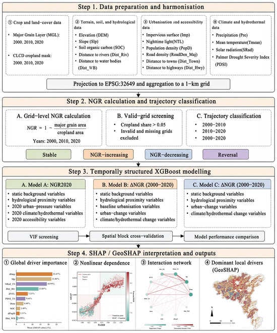
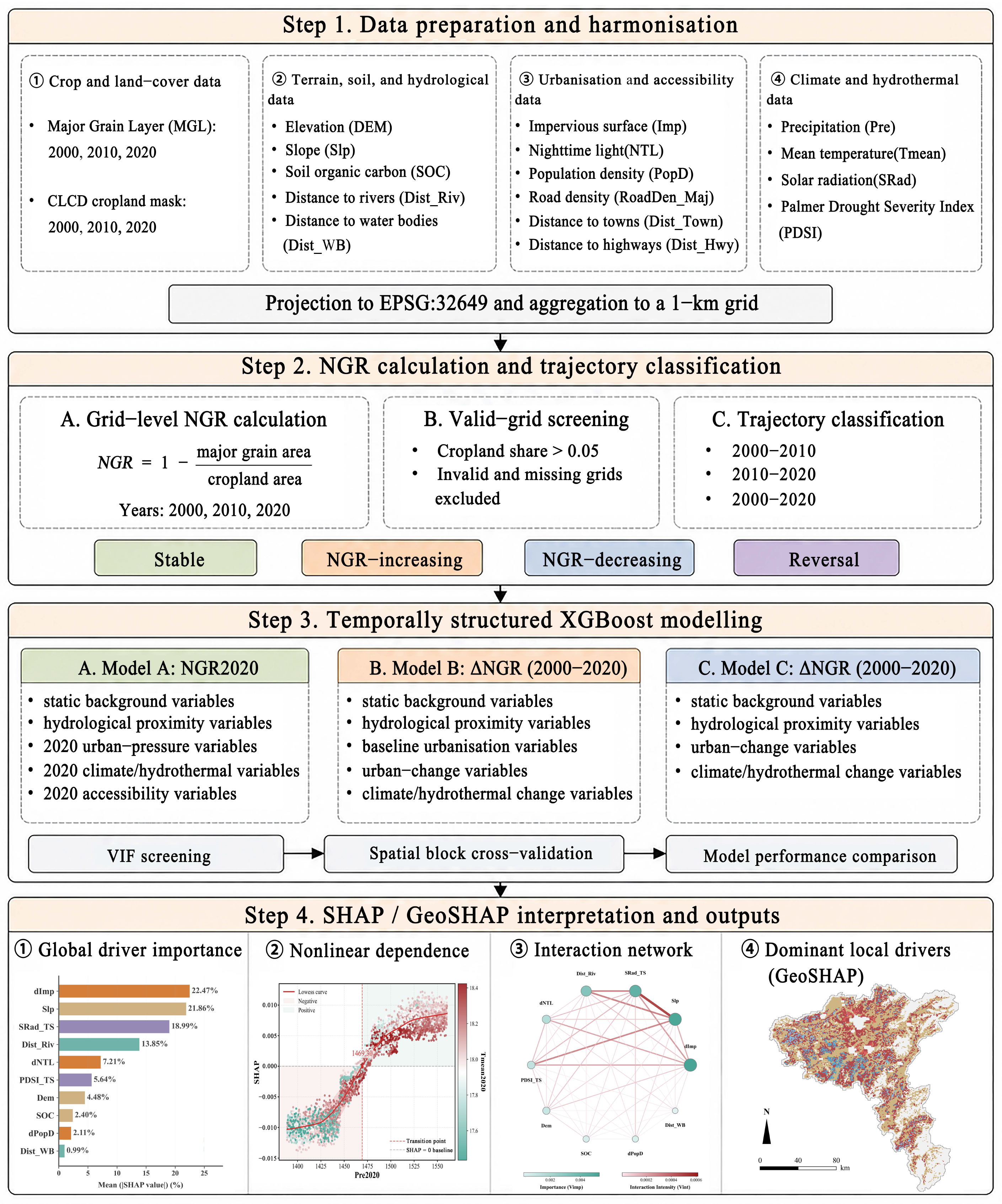
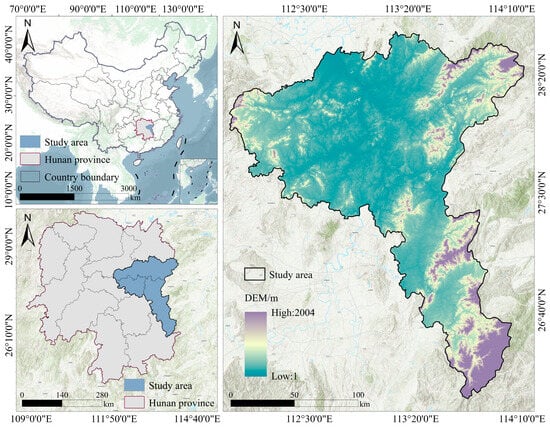
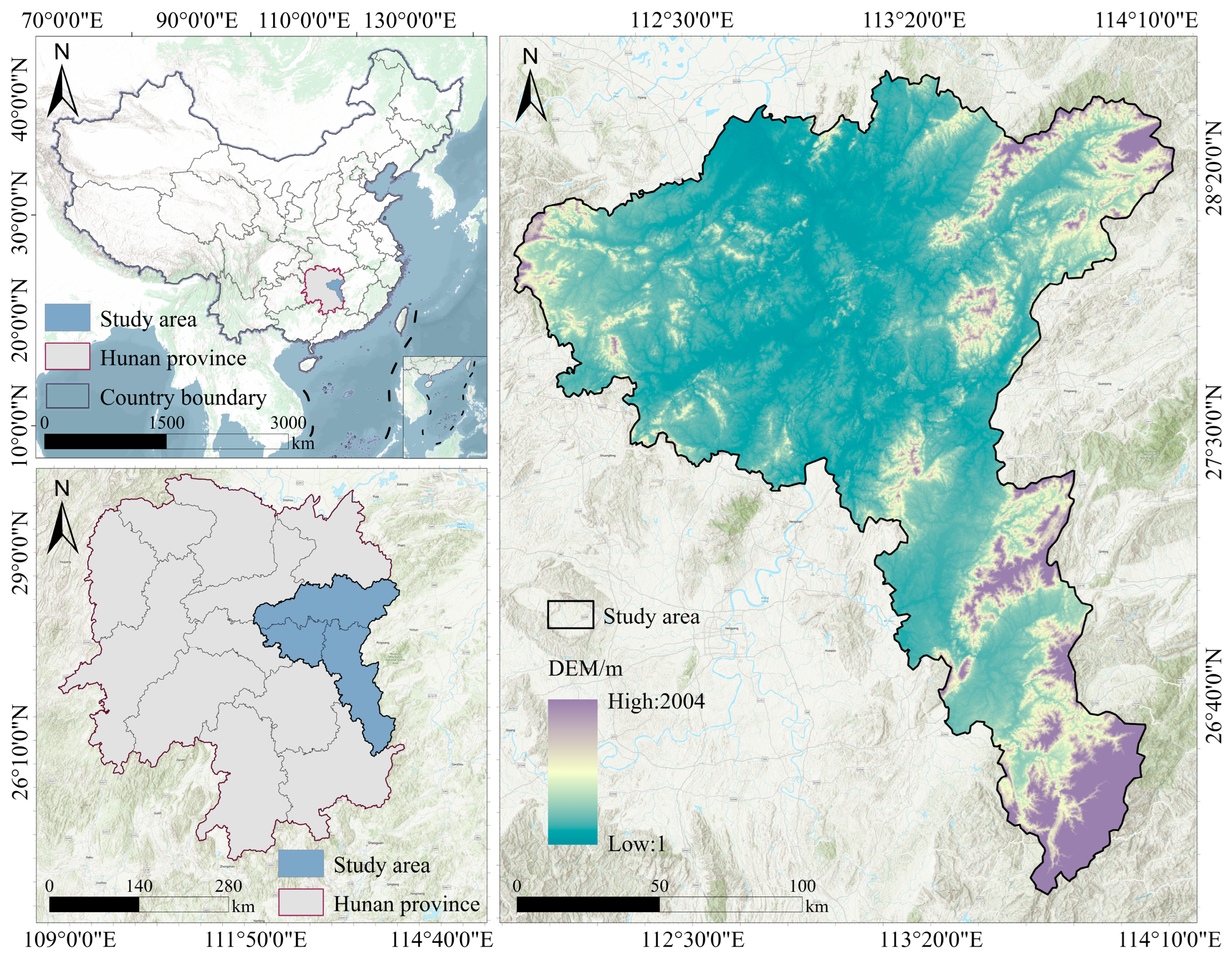
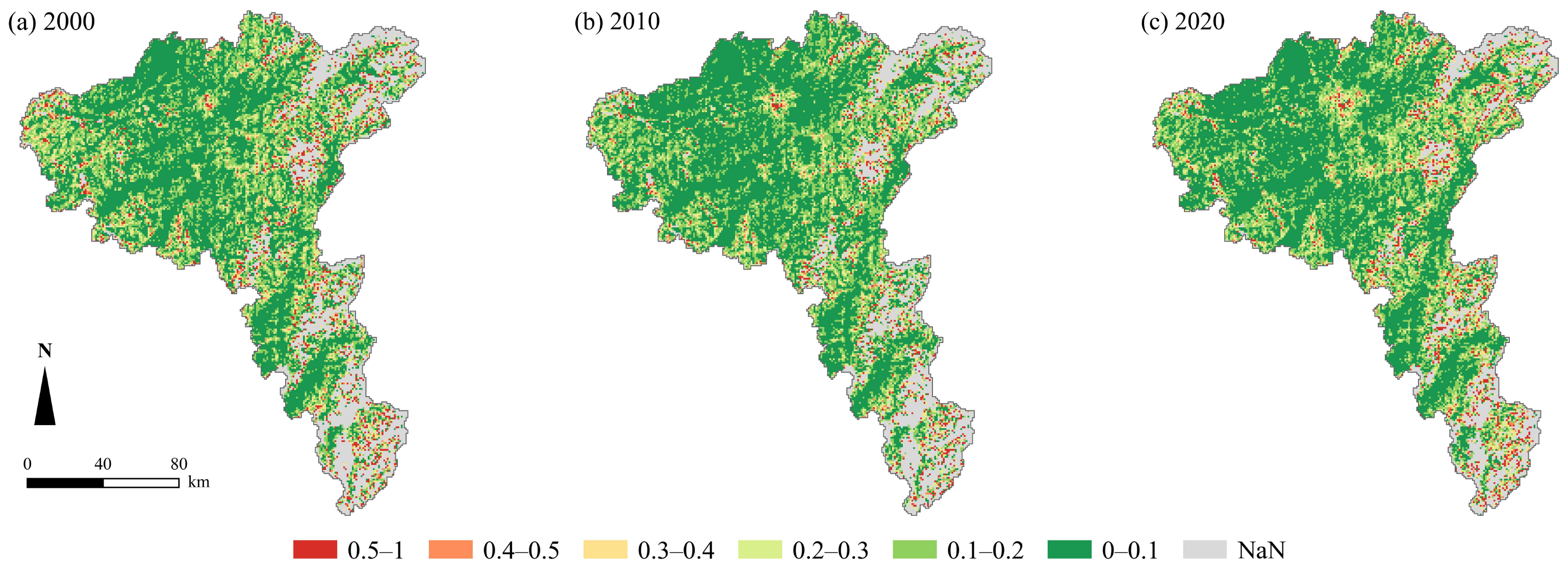
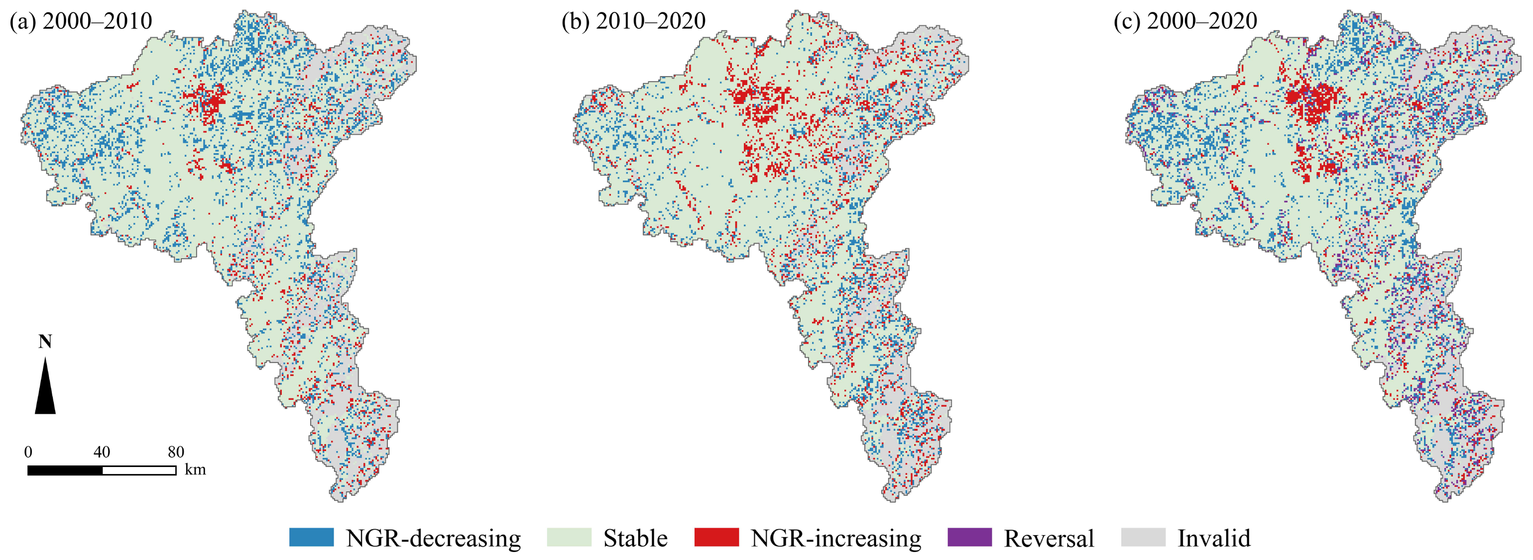
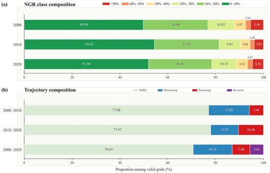
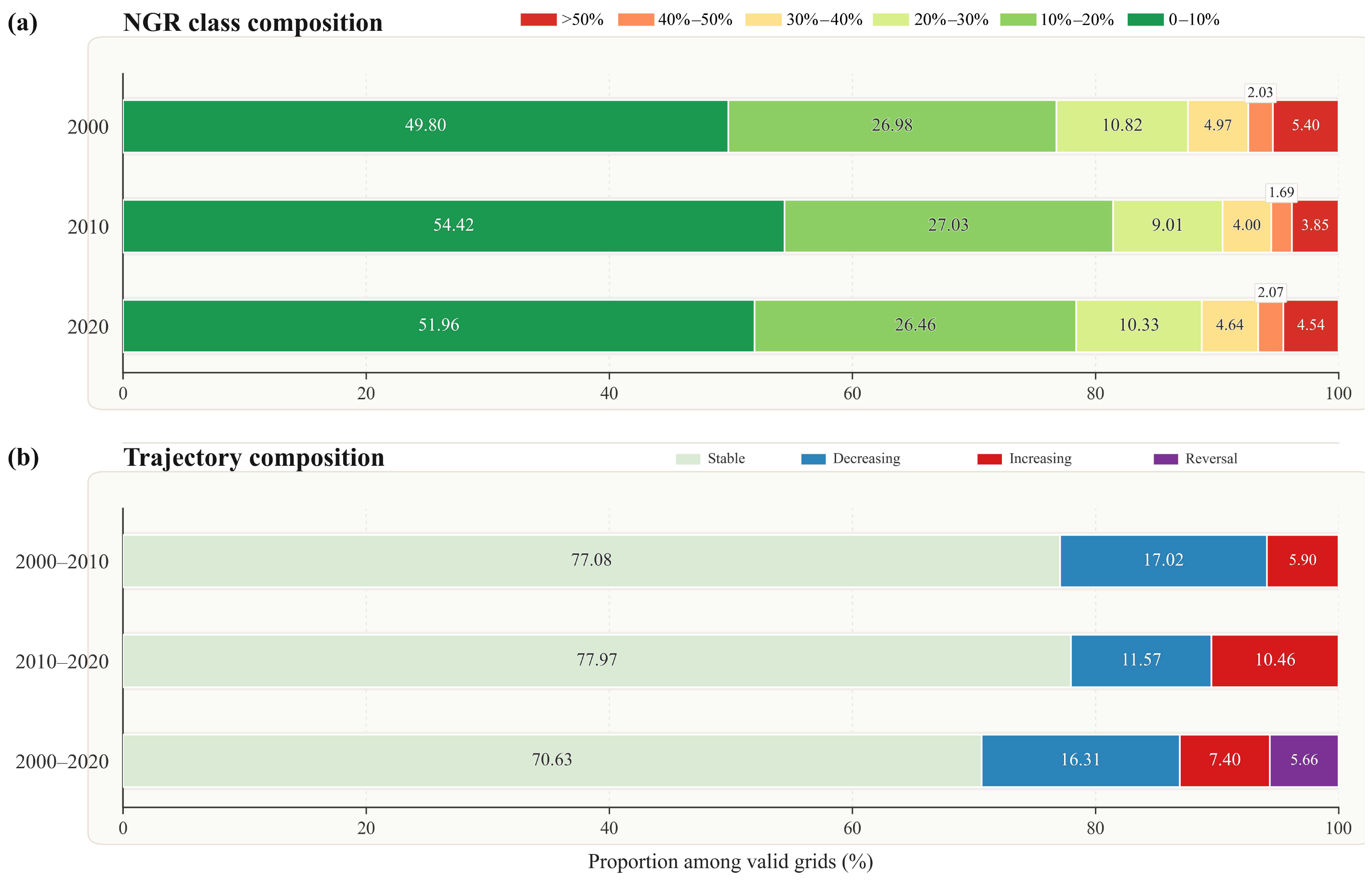
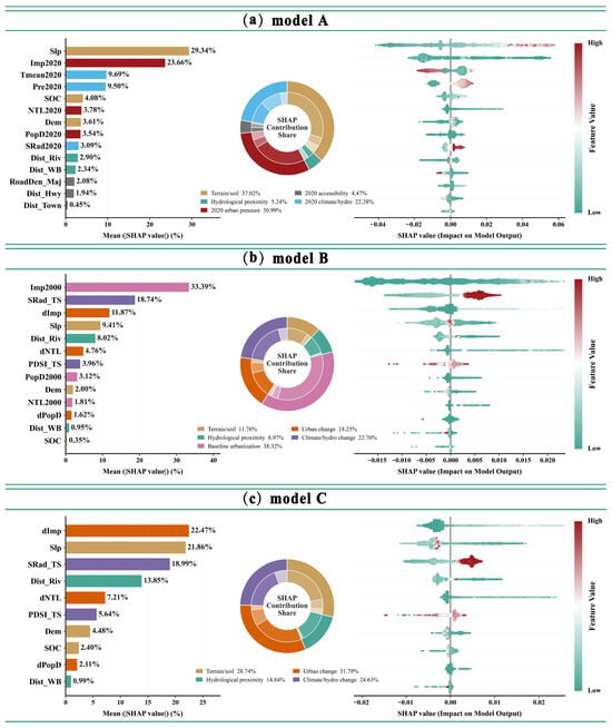
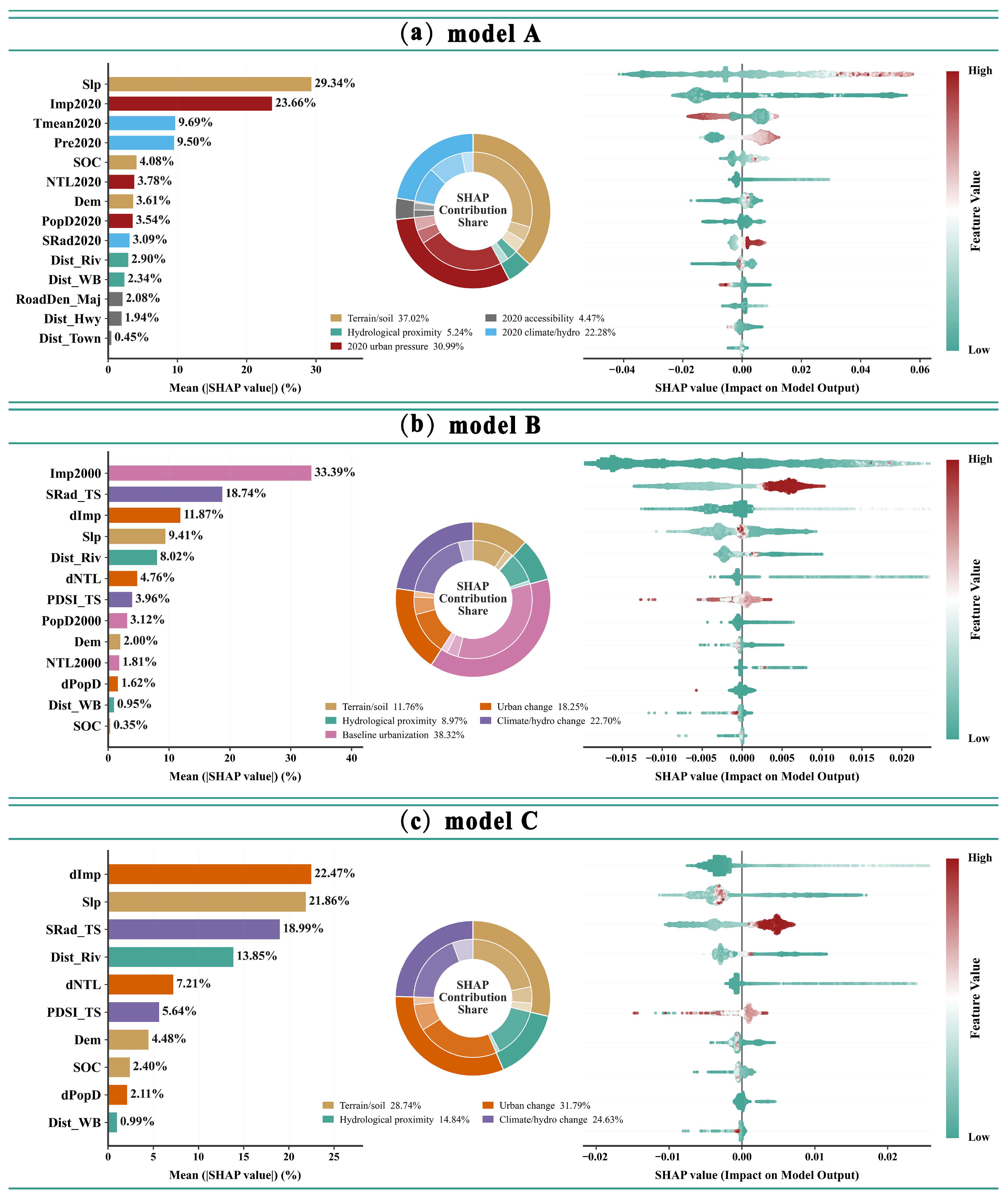
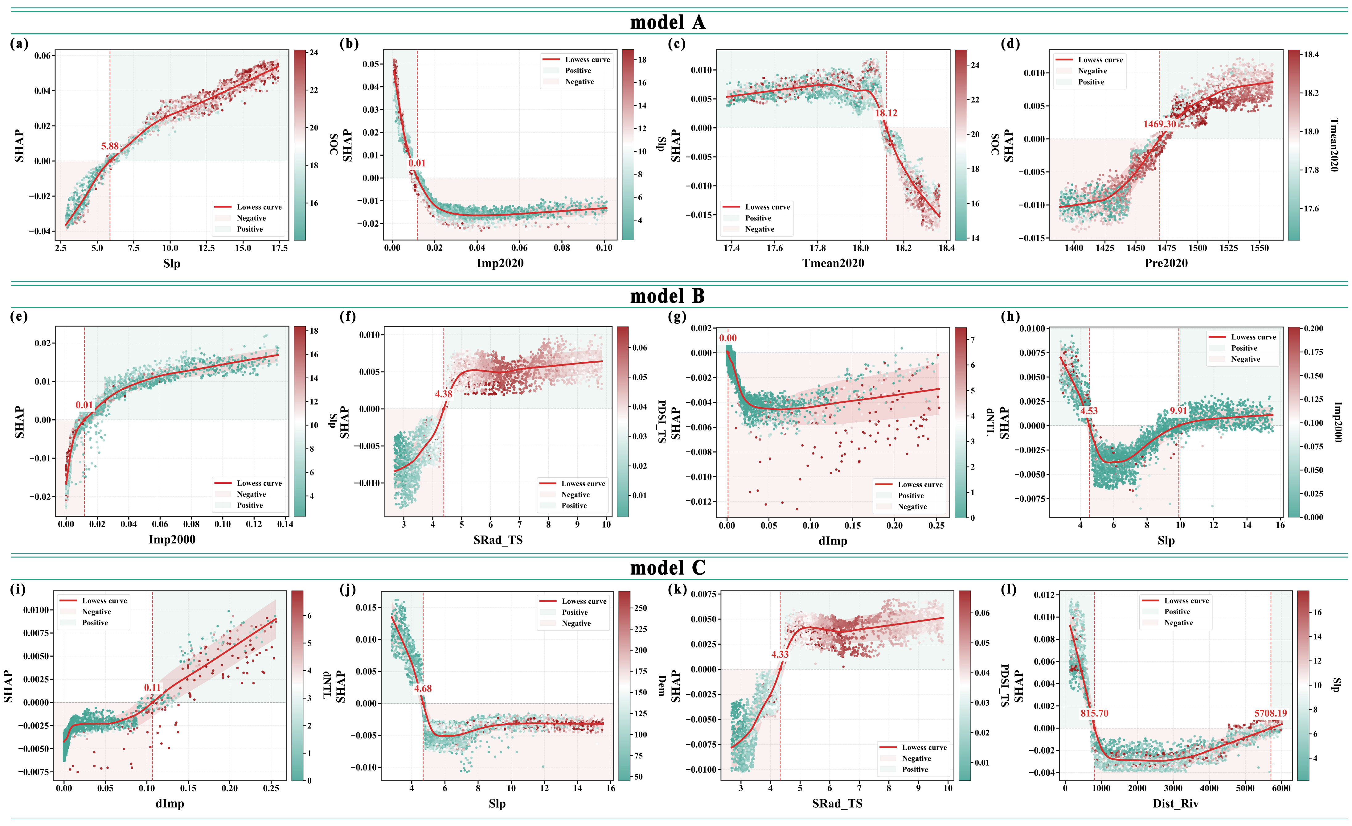
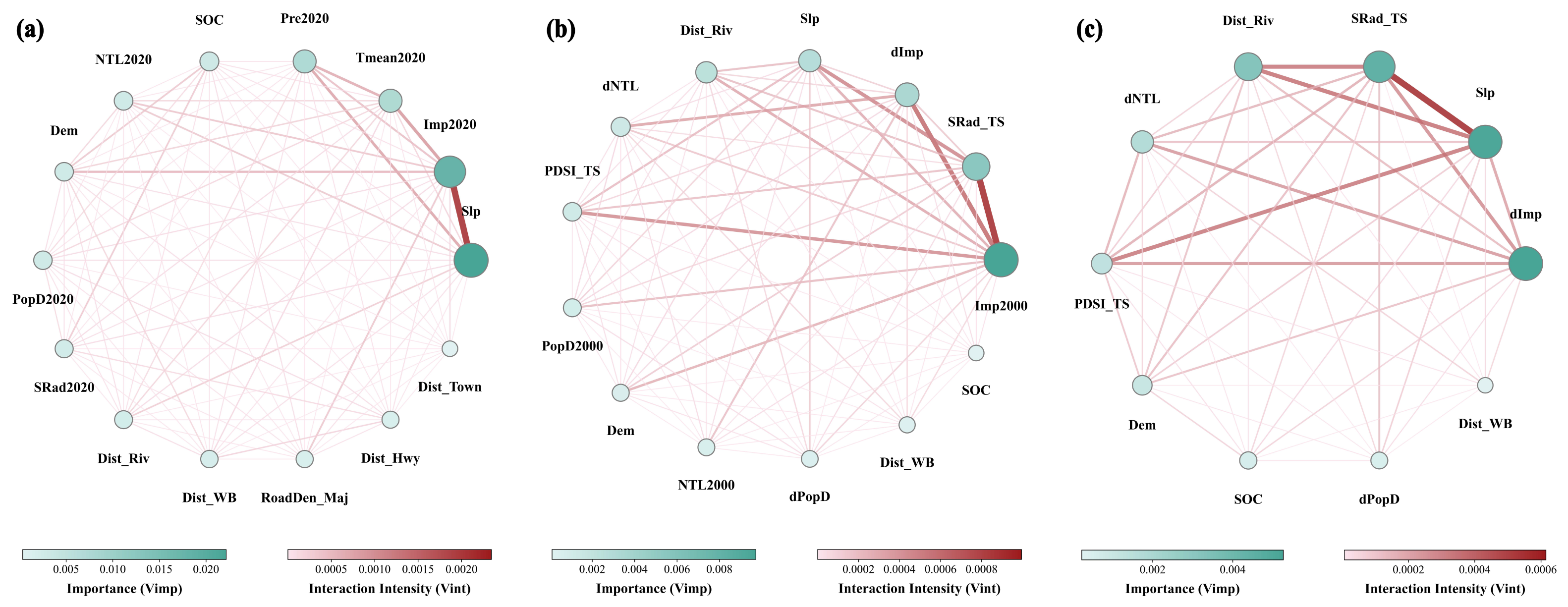
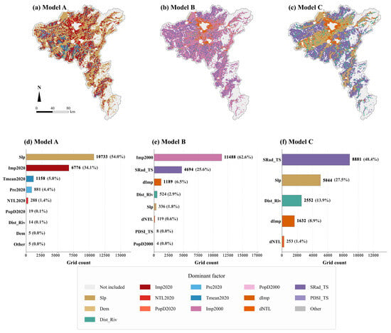
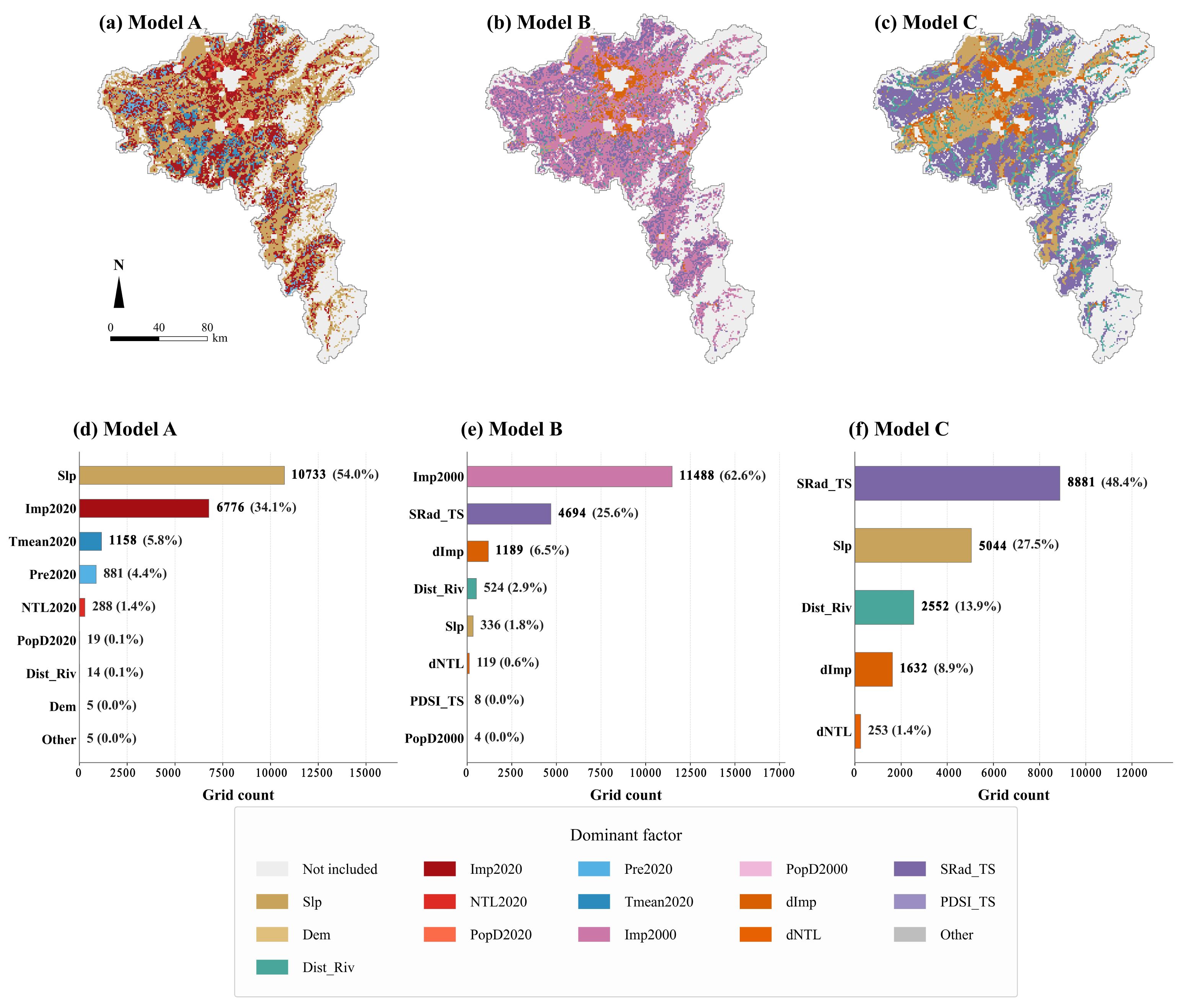

Disclaimer/Publisher’s Note: The statements, opinions and data contained in all publications are solely those of the individual author(s) and contributor(s) and not of MDPI and/or the editor(s). MDPI and/or the editor(s) disclaim responsibility for any injury to people or property resulting from any ideas, methods, instructions or products referred to in the content. |
© 2026 by the authors. Licensee MDPI, Basel, Switzerland. This article is an open access article distributed under the terms and conditions of the Creative Commons Attribution (CC BY) license.