


Abstract
Accurate estimation of residential building energy consumption and associated CO2 emissions is essential for refined urban carbon management. This study develops a hybrid framework that integrates physics-based simulation and machine learning to estimate residential building energy use and energy-related CO2 emissions in Shenzhen in 2020. Representative building archetypes were first simulated and then used to train machine-learning models for large-scale applications. Building-level energy estimates were further combined with a bottom-up inventory to generate high-spatiotemporal-resolution maps of residential CO2 emissions. The results show that: (1) the selected model achieved good accuracy and temporal robustness, with strong agreement between estimated and reference energy use at daily, monthly, and annual scales; (2) residential energy use was primarily driven by meteorological conditions, especially daily mean temperature and the duration of high-temperature conditions, and exhibited clear weekly and seasonal patterns, with higher values on weekends and in summer; (3) residential CO2 emissions in Shenzhen reflected the combined effects of scale and intensity, with Longgang and Bao’an contributing the largest total emissions, Self-built residential buildings contributing the largest aggregate emissions, and Old residential buildings showing the highest average emissions per building; (4) emissions were highly concentrated in a small number of high-emission buildings, which were more frequently distributed along road-adjacent block perimeters. Overall, the proposed framework improves the fine-scale characterization of residential building CO2 emissions and provides a useful basis for hotspot identification and targeted mitigation.
1. Introduction
In 2022, the total energy consumption from building operation and the construction sector in China reached 2.42 billion tons of standard coal equivalent (tce), accounting for 44.8% of the national total energy consumption. According to the report released by the China Association of Building Energy Efficiency, associated CO2 emissions amounted to 5.13 billion tons of CO2, representing 48.3% of the country’s energy-related CO2 [1,2]. China has pledged to achieve carbon peaking by 2030 and carbon neutrality by 2060. The building sector therefore holds considerable potential for carbon reduction, with an estimated 30% of emissions economically and efficiently reducible [3]. The reconstruction and fine-scale mapping of building operational energy consumption and emissions at high spatiotemporal resolution are crucial for formulating and implementing effective energy-saving and emission-reduction strategies [4,5], thereby providing essential support for achieving the twin goals [6].
Recent studies have shown that residential building energy use and carbon emissions exhibit strong intra-urban heterogeneity, making fine-resolution CO2 emission inventories and mapping increasingly important for targeted mitigation and spatially differentiated urban planning. Such datasets help to identify dominant emission sources, enable differentiated monitoring, and support targeted carbon-reduction strategies. This is particularly relevant in rapidly urbanizing cities, where mismatches among building stock, occupancy intensity, and cooling demand may lead to substantial variation in operational emissions within the same city [7,8].
Although recent studies have begun to address this issue using high-resolution mapping and city-scale modeling approaches, important gaps remain. For example, high-resolution mapping of urban residential carbon emissions has been implemented in Suzhou [9], while urban building energy models have been developed for Shanghai using multi-source open data [10]. In parallel, multimodal machine learning has demonstrated considerable potential for city-scale residential energy prediction [8]. However, fine-resolution daily estimates of residential energy-related carbon emissions at the building level remain scarce, particularly for rapidly urbanizing cities in southern China. Despite this growing demand, fine-resolution and long-term urban building energy and CO2 emissions datasets remain largely unavailable. In particular, historical building operational energy data and fine-resolution operational CO2 emissions datasets are still severely lacking at the city scale [11].
The bottom-up inventory approach is the carbon emission accounting method recommended by the IPCC guidelines. It estimates emissions based on statistics at the level of specific emission sources or activities, calculating carbon emissions using emission factors and activity data, and then aggregating them step by step to obtain the total emission results [12]. The spatialization of bottom-up carbon emission inventories derived from activity data is generally conducted through spatial downscaling based on spatial proxy data. Such proxy datasets generally represent spatial patterns of human activities and energy consumption intensity, including population distribution, mobile phone signaling data, and taxi trajectory records. In recent years, satellite-derived nighttime light data have also been widely validated as effective proxies for spatially allocating emissions. Representative bottom-up emission inventory systems include the Emissions Database for Global Atmospheric Research (EDGAR) [13] and the Open-Data Inventory for Anthropogenic Carbon Dioxide (ODIAC) [14].
However, due to the relatively long update cycles of statistical yearbook data, bottom-up approaches often struggle to satisfy the requirements for high-spatiotemporal-resolution estimation and analysis of building energy consumption and CO2 emissions [11]. In addition, considerable uncertainties arise in urban-scale applications [15,16], largely because these approaches depend heavily on proxy data for spatial allocation [4]. Consequently, the accuracy and representativeness of proxy datasets fundamentally constrain the reliability of bottom-up methods at finer spatial scales. To overcome these limitations, recent studies have increasingly combined physics-based simulation, urban building energy modeling, and machine-learning-based prediction to estimate building energy use and operational carbon emissions at finer scales [10,17,18]. These developments indicate a clear methodological shift from proxy-based allocation towards hybrid frameworks that more directly reflect building energy mechanisms.
Overall, existing research on urban building carbon emissions has mainly progressed along three strands. Studies of spatial carbon-emission patterns are useful for revealing intra-urban heterogeneity, but they often rely on proxy-based allocation and provide limited representation of underlying building-energy mechanisms. UBEM- or simulation-based studies offer a stronger physical basis for estimating building energy demand, yet they usually focus on energy estimation itself rather than fine-scale urban carbon-emission mapping. Machine-learning studies, in turn, have improved predictive performance for building energy or operational carbon estimation, but they often place greater emphasis on model accuracy than on spatially explicit carbon allocation and urban interpretation [9,10,17,18]. To address these gaps, this study develops a hybrid framework for Shenzhen that combines archetype-based physics simulation with machine-learning estimation to generate daily building-level residential energy use and then applies these estimates as spatiotemporal proxies for carbon-emission downscaling. By integrating these previously separate lines of research within a unified workflow, the study aims to improve the spatial representativeness, physical relevance, and interpretability of urban residential carbon-emission assessment in a dense subtropical megacity.
2. Materials and Methods
2.1. Study Area and Data Source
The study area is located in Shenzhen, Guangdong Province, China, which is characterized by a subtropical monsoon climate with mild winters, hot summers, and abundant precipitation (Figure 1). Shenzhen has a highly developed economy, and the strong concentration of population and economic activities has contributed to the growth of residential CO2 emissions. Meanwhile, as one of China’s first national low-carbon pilot cities, Shenzhen holds significant demonstrative value in carbon emission monitoring and the implementation of carbon-reduction policies.
Figure 1.
Study area. District boundaries were based on the standard Shenzhen administrative map (non-neighboring-district version) from the Shenzhen Geospatial Information Public Service Platform.
The Typical Meteorological Year (TMYx) data covering the period 2009 to 2015, together with the actual meteorological year (AMY) data for 2020, used in this study were obtained from Oikolab “oikolab.com (accessed on 2 July 2024). Building vector data for Shenzhen were obtained from the Global Building Atlas [19]. Building function classifications and other attribute information were extracted from Open Street Map point-of-interest data, while building height information was derived from the Chinese Building Height dataset at 10 m spatial resolution [20].
As of the end of 2020, Shenzhen had a permanent resident population of 17.6338 million, with a male-to-female ratio of 1.22:1, and 80% of the population was aged 15–59. Based on the GBA dataset, Shenzhen contained 573,399 buildings in 2020, of which 424,077 were associated with residential use. The total building footprint area was 213.60 km2, with an average building area of 372.30 m2. District-level statistics on population, number of buildings, and building footprint area are presented in Table 1.
Table 1.
Comparative statistics of building emissions within buffer zones.
In terms of total building count, Longgang District ranks highest with 116,388 residential buildings and records the largest total floor area of 2356.05 km2. This is followed by Bao’an District, which has 109,077 residential buildings with a total floor area of 1756.03 km2.
As shown in Figure 2, among different building types, MRB and SR buildings dominate in both quantity and total floor area. Across the entire city, there are 341,937 SR buildings with a total floor area of 3122.34 km2, and 36,311 MRB buildings with a total floor area of 3733.82 km2. Although SR buildings are far more numerous, they are typically low-rise with smaller footprints. In contrast, MRB buildings generally have greater heights and larger floor areas, resulting in a higher total floor area despite having nearly an order of magnitude fewer buildings than SR types.
Figure 2.
Total floor area by district and building type.
2.2. Methods
The study first performs physics-based simulations to estimate the energy consumption of typical residential buildings in Shenzhen. Based on these simulations, machine-learning models are trained using meteorological variables, building geometric parameters, and temporal features to estimate the daily energy consumption of residential buildings across the entire city. The resulting energy consumption estimates are then used as spatial proxy data for bottom-up spatial allocation, enabling estimation of CO2 emissions from residential buildings throughout Shenzhen.
2.2.1. Physics-Based Modeling and Simulation
The selection of typical buildings, the specification of envelope constructions, and the definition of occupant-related disturbances are key determinants of the accuracy of building energy consumption simulations performed using EnergyPlus V24-1-0. To ensure that the model inputs accurately reflect local building characteristics, a comprehensive on-site survey was conducted in Shenzhen at the end of 2023, covering major residential areas across multiple districts, including Luohu, Futian, Nanshan, Bao’an, Longgang, and others. Based on the findings of field surveys, we classified residential buildings into five representative types, considering factors such as architectural form, mixed-use functions and construction period, as illustrated in Figure 3.
Figure 3.
Prototype and modeling of typical residential building in Shenzhen.
UTR denotes a typical urban townhouse residential typology widely constructed between the 1980s and 2000s, characterized by modular and symmetrically arranged dwelling units, flexible layouts, and a predominantly north–south orientation. MUR denotes a mixed-use residential building type commonly found in southern Chinese cities, characterized by a commercial podium on the lower floors and residential units above. To reflect this mixed-use configuration, the commercial and residential parts of MUR were modeled separately in this study, with the commercial portion assumed to occupy one floor in buildings with 12 stories or fewer, and two floors in buildings with more than 12 stories. MRB and ORB both denote tower-form pure residential buildings. The main distinction between them lies in construction period and thermal performance: ORB generally represents older residential buildings with relatively poorer thermal performance, higher solar heat gains, and higher heat transfer coefficients, whereas MRB represents newer and more modern residential configurations. SR denotes a typical self-built residential type commonly found in urban villages across southern China. This type is characterized by very high building density, narrow spacing, and street-facing daylight access and is further associated with higher occupant density and poorer thermal performance than other residential types.
The building envelope and associated parameters were specified mainly based on the national standard General Code for Energy Efficiency and Renewable Energy Utilization in Buildings (GB 55015-2021), with further adjustments informed by the Shenzhen local standard and previous studies in relevant regions. Details of these settings are presented in Appendix A, Table A2. In total, 336 valid questionnaires were collected during the field survey, comprising 116 paper-based responses and 220 online submissions. These data provide valuable insights into residential conditions and occupant living habits in Shenzhen. Combining the GB 55015 standard with relevant local codes for building simulation, a generalized occupant schedule was developed and used as the basis for modeling occupant-related disturbances; details of the occupant schedule are presented in Appendix A, Figure A3.
The Open Studio was employed to develop three-dimensional models for the five typical building types. To enhance the generalizability of the simulation results, the internal spatial configurations were simplified, with each room represented as a single thermal zone (see Figure 3). Furthermore, a series of multi-story models were batch-generated for different building types, ranging from single-story structures to high-rise buildings of up to 33 floors, to support large-scale energy consumption simulations. A total of 126 building models were generated in this process.
The meteorological data utilized for EnergyPlus simulations was sourced from the TMYx meteorological dataset provided by Oikolab for the Shenzhen International Meteorological Station (ID 594930). All simulations were conducted with a daily time step, and the setpoint temperature of the air-condistioning equipment was fixed at 26 °C, consistent with the operational mode identified from the preliminary survey data.
2.2.2. Machine-Learning Models
Prior to model training, a systematic data quality control and preprocessing workflow was applied to the simulated building energy consumption outputs. Outliers in the daily energy-use intensity (DEUI) dataset, accounting for 0.10% of the observations, were identified and excluded using the Z-score criterion (∣Z∣ ≥ 3). Subsequently, missing values were imputed by assigning the median DEUI value of the corresponding building type for the same calendar day.
Based on an in-depth examination of the statistical characteristics and physical interpretations of the source parameters, additional derived features were constructed to enhance the model’s explanatory capacity. New engineering variables such as high duration, CDD, and day of year have been incorporated to capture both the climatic responsiveness and temporal periodicity of building energy consumption. The definitions and meanings of all feature parameters are summarized in Table A1.
A systematic feature selection procedure was implemented using feature importance measures and the correlation coefficient matrix. Figure A1 presents the visualization of feature importance and the correlation matrix. Feature selection was guided by two principles: (a) the selected features should encompass building, meteorological, and temporal feature clusters and sufficiently represent their key characteristics; (b) among highly correlated variables, features with higher importance and greater data availability were prioritized. Accordingly, the final set of features includes temp mean, high duration, RH mean, GHrad sum, is weekend, doy sin, doy cos, building type, building area and floor.
To capture the complex and nonlinear interactions among meteorological variables, building characteristics, and energy consumption, this study employed and systematically evaluated a series of machine-learning algorithms. The models used include linear models such as Ridge, Lasso, and Elastic Net; bagging-based tree models such as Decision Tree and Random Forest; and boosting-based ensemble models including Gradient Boosting Machine (GBM), LightGBM, CatBoost, and XGBoost.
Since daily building energy consumption data exhibit strong temporal dependencies, the time-block partitioning strategy was employed to ensure that model evaluation accurately reflects the true performance of time-series data. In this method, the entire dataset was divided along the temporal axis into fixed-length training and testing blocks. In each fold, the training set includes all observations preceding the current testing period, while the testing set consists of the subsequent time segment. A schematic illustration of this procedure is provided in Figure A2. All building samples are synchronously partitioned across identical time intervals, ensuring that both training and testing blocks contain data from the same temporal span for all buildings and avoiding information leakage from the future.
Based on the time-block partitioning strategy, the dataset was divided into multiple folds, and the average values of the evaluation metrics across folds were used to represent model performance under this partitioning scheme. To ensure the robustness and generalization capability of model evaluation, all models were tested under various combinations of training and testing window lengths. Specifically, the initial training window ranged from 28 to 182 days, with an increment of 7 days, while the testing window varied from 7 to 28 days, also in 7-day increments.
Within each training fold, hyperparameters were optimized using an adaptive inner expanding-window cross-validation scheme combined with Halving Random Search CV, where RMSE served as the primary selection criterion. This successive-halving search strategy enabled efficient exploration of model-specific hyperparameter spaces while progressively allocating computational resources to better-performing candidates. The final predictive performance of each model was assessed over all outer folds using R2, RMSE, and MAE and summarized by both mean and standard deviation to capture accuracy as well as temporal stability.
2.2.3. Model Interpretation and Feature Contribution Analysis
Explainable machine-learning models have attracted growing interest because they can quantify the contributory effects of individual features on model estimations, thereby improving transparency and interpretability. The theoretical foundation of the SHAP (SHapley Additive exPlanations) framework is rooted in the concept of Shapley values from cooperative game theory [21], which enables the equitable attribution of marginal contributions to each feature while adhering to the axioms of fairness and consistency.
The SHAP value for feature , denoted as , is defined as the weighted average of the marginal contribution of feature across all possible feature subsets that do not include :
where represents the full set of input features, denotes a subset of features excluding , and is the model output function.
Based on the SHAP framework, the output of a machine-learning model for a given sample can be expressed as an additive decomposition:
where is the expected model output over the background dataset, and quantifies the contribution of the -th feature to the deviation of the output from this baseline.
2.2.4. Model Estimation
Building energy consumption generally consists of two components: baseline load and occupant-related load. The baseline load refers to the energy consumed when the building is unoccupied, including standby equipment power, public lighting, server-room loads, and the basic operating load of HVAC systems. The occupant-related load varies with the number of occupants and their behavioral patterns. Without adjusting the simulation outputs for occupant density and occupancy rate, the full-occupancy assumption would inevitably lead to an overestimation of energy use [22,23]. Thus, modeling and correcting for occupancy and its associated factors is a critical step in aligning simulation results with real-world building performance.
We employ an Occupancy Intensity Coefficient to adjust the estimation results. This coefficient reflects the deviation of actual occupancy from the full-occupancy assumption and enables an appropriate correction of the occupant-related load component. The adjustment is calculated as follows:
where denotes the adjusted energy consumption, represents the simulated energy consumption estimated by the physical model, denotes the actual occupancy rate (i.e., the ratio of actual to design population), and represents the proportion of baseline energy consumption.
The coefficient is typically computed as the ratio of actual occupancy to design occupancy. The design occupancy is estimated using the building floor area divided by the per-capita floor area. According to the Sixth National Population Censuses, the per-capita floor area in Shenzhen is 27.8 m2. The actual occupancy is determined from the WorldPop dataset by extracting the population counts within the spatial extent of each building.
Following occupancy-aware energy baseline modeling, total building energy use can be interpreted as the sum of an occupancy-insensitive baseline component and an occupancy-responsive component, and the corresponding baseline fraction can be treated as a calibration or adjustment parameter when occupancy information is introduced [24]. In the present study, is therefore defined as a type-specific baseline-load fraction rather than a universal constant. Building on the approach of Liang et al. [24] and further informed by our questionnaire survey, the parameter was specified for different building types. Questionnaire results further suggest that SRs exhibit stronger energy-saving behavior and own fewer basic appliances, whereas MURs generally retain higher common-service and standby loads. Accordingly, β is set to 0.4 for MUR, 0.2 for SR, and 0.3 for other types. To reduce the influence of anomalous population values, the final adjustment coefficient is constrained to the range [0.2, 1.2].
2.2.5. Spatiotemporal Downscaling
The annual CO2 emissions are accounted for using the inventory-based methodology recommended by the IPCC, which relies on sectoral statistical data. CO2 emissions associated with energy consumption and industrial production processes are calculated according to inventory items disaggregated by sector and fuel type, together with their corresponding emission factors. The emissions are calculated using the following formula:
where represents the 47 industry sectors classified in the IPCC guidelines, stands for the 17 major types of fossil fuels as classified in the guidelines, represents CO2 emissions of industry from the combustion of energy source , and means the CO2 emissions generated by the corresponding industrial process . means the denotes the consumption of the corresponding energy source, and represents the CO2 emission factor associated with that energy source.
To ensure consistency between estimated results and statistical records, downscaling methods were employed to disaggregate annual CO2 emissions derived from statistical data into daily, building-level values. Using the adjusted building energy consumption values as weighting factors, daily building-level CO2 emissions were computed accordingly, as follows:
where denotes the CO2 emissions of building on day , represents the total annual CO2 emissions of the building sector, and denotes the adjusted building energy consumption value of building on day .
2.2.6. Validation
This study proposes two complementary validation approaches—one at the individual-building level and the other at the annual total emission level—to assess the plausibility and reliability of the model results.
At the individual building level, type-specific average energy intensity values were directly employed to derive building energy consumption estimates. This approach builds on the methodology developed by Liu et al. [25], who demonstrated, using data from Dongguan, that an average energy intensity-based method yielded R2 values ranging from 0.72 to 0.83 for urban residential buildings, urban village buildings, and commercial buildings. These results indicate the applicability of this method in the Pearl River Delta region, and it was therefore employed to validate the estimated energy consumption of individual buildings.
Specifically, for the five typical building types, physics-based simulations were re-performed using the actual meteorological conditions of the target year. Building energy consumption was then derived using the average DEUI value for each building type together with the corresponding building floor area. Subsequently, 50 buildings were randomly selected from each category, yielding a sample of 250 buildings with complete annual energy consumption records. Model calibration and performance assessment were then performed at daily, monthly, and annual temporal scales, respectively.
Second, a validation was conducted from an aggregate perspective. Using the estimation energy consumption and the 2020 Guangdong provincial grid emission factor (0.445 kg CO2/kWh), the annual total CO2 emissions of Shenzhen’s building sector for the year 2020 were estimated. This estimate was then compared against the building sector CO2 emissions derived from official statistical data, enabling an assessment of the model’s consistency and reliability at the citywide scale.
The equation is formulated as:
where denotes the annual total energy consumption of building , represents the grid emission factor, and denotes the annual total CO2 emissions of the building sector.
3. Results
3.1. Hybrid Model Results
3.1.1. Physics-Based Simulation Results
The green dashed line in Figure 4a represents the average DEUI variation across all building types. The energy-use intensity of buildings exhibits pronounced seasonal and periodic patterns. The periodic variation is primarily manifested in the weekly cycle of DEUI, with residential buildings exhibiting higher DEUI on weekends than on weekdays. Regarding seasonality, Shenzhen has a subtropical monsoon climate characterized by hot summers and mild winters, with an extended period of high temperatures. The warming period typically begins in April and lasts until November, and temperatures seldom drop below 10 °C throughout the year. From early May to mid-October, the monthly average temperature remains above 25 °C for nearly half a year, leading to a significant increase in cooling demand and, consequently, higher DEUI.
Figure 4.
(a) Typical building energy simulation results under TMY conditions. (b) Monthly variation in the share of cooling energy consumption in typical buildings.
The boxplots in Figure 4a illustrate the monthly distribution of DEUI across different building types. Both UTR and SR exhibit substantially higher DEUI levels compared with the other three categories. SR shows markedly larger median values, wider interquartile ranges, and more pronounced extremes. These differences become even more evident during the high-temperature period from May to October.
Figure 4b presents the average proportion of cooling energy consumption in the total daily energy use across different building types. During December, January, and February, cooling demand is minimal, and building energy use is primarily driven by equipment, lighting, and other non-cooling loads. As the average temperature rises, the share of cooling energy consumption increases steadily, reaching nearly 90% between June and September. This indicates that during the summer period, building energy use is dominated almost entirely by cooling demand.
3.1.2. ML Model Comparison
The R2 performance of all models under different combinations of initial training and testing windows is illustrated in Figure 5. Different combinations of the initial training window and testing window have a considerable impact on the performance of the models. As the length of the initial training window increases, the overall performance of the models generally improves, although slight fluctuations can still be observed. The optimal performance of most models is achieved when the initial training window exceeds approximately 140 days, with a testing window of 21 or 28 days.
Figure 5.
Comprehensive heatmap of model R2 comparison; (a–d) correspond to test window sizes of 7, 14, 21, and 28 days, respectively. Within each panel, the color gradient represents the R2 value, showing the performance of each model as the initial training window gradually increases. The blank areas marked with “--” indicate cases where the model performance is worse than that of the mean prediction baseline.
In terms of overall model performance, comparison of the average R2 values indicates that the models with ensemble learning, such as GBM (0.739), CatBoost (0.735), and XGBoost (0.723), substantially outperform the linear models Ridge, Elastic Net, and Lasso in this energy consumption estimation task. This suggests that the relationship between the feature variables and building energy-use efficiency is far more complex than can be captured by linear formulations. In contrast, the performance of basic tree-based models such as Decision Tree and Random Forest is relatively modest, falling short of the estimation accuracy achieved by the ensemble approaches.
The CatBoost model achieves the best overall performance among all models and window configurations when using a training window of 182 days and a testing window of 21 days, yielding R2 = 0.879, RMSE = 0.0092, and MAE = 0.00686. Considering both estimation accuracy and computational efficiency, CatBoost was ultimately selected as the final model for building-level daily energy consumption estimation.
3.2. Feature Analysis
The SHAP summary beeswarm plot shown in Figure 6 illustrates the global feature contribution patterns of the model, addressing the question of which features are most important. The SHAP dependence plots for individual features further reveal the functional relationships between these key variables and energy consumption, explaining how each feature influences the estimation. Overall, meteorological variables constitute the primary drivers of the model’s estimations, exerting substantially greater influence than temporal features and building physical attributes.
Figure 6.
SHAP dependence plots for individual features. (a) Summary beeswarm plot of SHAP. (b–i) Dependence plots for each individual factor.
Daily mean temperature is identified as the most influential factor affecting final building energy consumption, followed by the duration of high-temperature conditions. Both features exhibit positive monotonic relationships and clear threshold effects. Specifically, when temperature or high-temperature duration exceeds certain critical values, the SHAP values rapidly become positive and increase significantly with further rises in temperature.
The impact of weekday–weekend consumption patterns on building energy use is more pronounced than that of seasonal variations. Significant differences are observed between weekends and weekdays: weekends tend to increase building energy consumption, whereas weekdays generally suppress its growth.
Among building types, UTR and SR buildings are associated with increased energy consumption, whereas the remaining building types exhibit a slight suppressing effect on energy use. The SHAP curve for building area shifts from positive to negative contributions, suggesting that smaller buildings tend to have higher daily electricity consumption, while the marginal effect diminishes as floor area increases. This likely reflects larger residential units having greater per-capita floor area, more shared or non-conditioned spaces, and cooling loads that do not scale proportionally with total floor area.
In addition, global horizontal irradiance, relative humidity, and the number of floors all exhibit positive monotonic effects on building energy consumption.
3.3. Spatiotemporal Distribution
3.3.1. Total CO2 Emissions by District
Figure 7 illustrates the spatiotemporal distribution of CO2 emissions from the building sector in Shenzhen for the year 2020 following the downscaling correction. From the perspectives of district-level emission characteristics, building-type emission characteristics, and their combined patterns, residential building carbon emissions in Shenzhen in 2020 consistently demonstrated the coexistence of scale and intensity effects. Longgang District exhibits the highest annual building-related CO2 emissions, followed by Bao’an, Longhua, Nanshan, and Futian. Annual emissions in Longgang reached 1.119 million tons of CO2, accounting for 22.6% of the city’s total, while emissions in Bao’an also exceeded 0.954 million tons of CO2. In contrast, the lowest building CO2 emissions were observed in Yantian (0.067 million tons of CO2) and Dapeng (0.054 million tons of CO2). This spatial pattern of emissions is broadly consistent with the total floor area of each district and the distribution of population density across districts. In 2020, Bao’an recorded the largest permanent resident population (4.491 million), followed by Longgang (3.999 million) and Longhua (2.543 million).
Figure 7.
Spatiotemporal patterns of building CO2 emissions in Shenzhen, 2020. The pie chart illustrates the distribution of high-emission buildings with annual CO2 emissions exceeding 50 tons among different districts, while the table below summarizes the total annual building CO2 emissions in each district.
The divergence between total emission patterns and average emissions per building suggests that the higher total residential building carbon emissions in districts such as Longgang, Bao’an, and Longhua were primarily driven by the large number and greater scale of buildings, indicating a clear scale effect. By contrast, although districts such as Futian, Nanshan, and Luohu exhibited relatively lower total emissions, the concentration of high-rise, large-scale, and functionally more complex buildings led to markedly higher emissions at the individual-building level, revealing a typical intensity effect. This spatial pattern is consistent with the distribution of high-emission buildings—defined as those emitting more than 50 tons of CO2 annually—across these districts, as illustrated by the pie chart in Figure 7.
The frequency distribution of building carbon emissions in Shenzhen in 2020 (Figure 8) further demonstrates that residential building carbon emissions across the city exhibited a markedly asymmetric distribution, with a small number of high-emission buildings exerting a substantial influence on both the overall distribution pattern and the aggregate emission level. Specifically, the citywide sample comprised 424,077 residential buildings, with total annual carbon emissions of approximately 4.96 Mt CO2. The mean annual emission per building was 11.696 t CO2, whereas the median was only 2.289 t CO2, indicating that the majority of buildings were concentrated within a relatively low emission range. The quantile results further reveal a right-skewed, long-tailed distribution: the 75th percentile was only 7.480 t CO2, while the 90th percentile increased to 18.911 t CO2, and the 95th and 99th percentiles rose sharply to 35.766 t CO2 and 181.657 t CO2, respectively.
Figure 8.
Frequency distribution chart of annual carbon emissions from buildings.
The substantial gap between the mean and the median indicates significant stretching at the upper end of the distribution, with a small group of ultra-high-emission buildings forming a highly prominent tail. This pattern is further reflected in the concentration of emission contributions: the top 1% of emitting buildings accounted for approximately 38.70% of total annual carbon emissions, the top 5% contributed about 61.65%, and the top 10% accounted for around 72.75%. These findings suggest that annual carbon emissions from residential buildings in Shenzhen were highly concentrated in a limited number of high-emission buildings, which not only shaped the overall distributional pattern but also played a dominant role in determining the citywide total, thereby making them the key targets for future priority emission reduction and refined carbon management.
3.3.2. CO2 Emission Variations Across Building Types
The annual carbon emissions of different building types exhibited the coexistence of scale and intensity effects (Figure 9). In terms of aggregate emissions, SR buildings were the largest contributor to residential building carbon emissions in Shenzhen, with annual emissions of approximately 2.150 Mt CO2 in 2020, followed by MRB (1.338 Mt CO2), ORB (0.600 Mt CO2), MUR (0.556 Mt CO2), and UTR (0.317 Mt CO2). However, from the perspective of average emissions per individual building, ORB buildings recorded the highest annual carbon emissions, at approximately 69.541 t CO2, significantly exceeding those of other types, while MRB and UTR also remained at relatively high levels, at 36.852 t CO2 and 33.618 t CO2, respectively. In contrast, SR buildings averaged only 6.287 t CO2, the lowest among the major building types. These results suggest that although SR buildings had relatively low per-building emission levels, their very large stock made them the dominant contributor to total emissions, reflecting a typical scale effect; by contrast, ORB, MRB, and UTR were more characteristic of high-intensity emissions.
Figure 9.
Annual CO2 emissions by building type. (a) Total and mean annual CO2 emissions for each building type. (b–f) Distributions of annual CO2 emissions for UTR, MUR, MRB, ORB and SR.
To test differences in carbon emissions among building types, Kruskal–Wallis tests were conducted for annual carbon emission per building, annual carbon emission intensity per unit area, and peak-month carbon emission, followed by pairwise Mann–Whitney U tests with Holm correction (Figure 10). Significant differences were found among building types for all three indicators: annual emission (H = 29,199.134, p < 0.001), annual emission intensity (H = 61,636.258, p < 0.001), and peak-month emission (H = 29,466.307, p < 0.001). All 10 pairwise comparisons among the five building types were significant after Holm correction (p < 0.05).
Figure 10.
The difference in carbon emissions among building types. (a) Kruskal–Wallis test results for overall group differences among building types for three metrics: annual CO2 emission, annual CO2 emission intensity, and peak-month CO2 emission. (b) Distribution of annual building-level CO2 emissions by building type. (c) Distribution of annual building-level CO2 emission intensity by building type. (d) Distribution of peak-month building-level CO2 emissions by building type.
Based on median values, annual emissions per building and peak-month emissions showed the same ranking, ORB > UTR > MRB > SR > MUR, whereas annual emission intensity per unit area followed SR > MRB > UTR > MUR > ORB. These results indicate that building type significantly affects not only total emissions, but also emission intensity and peak-period emission levels.
3.3.3. Analysis of the Daily Trends in CO2 Emissions
Residential building CO2 emissions in Shenzhen exhibited clear temporal regularity at both short and long timescales. As shown in Figure 11a,b, residential building CO2 emissions exhibited a stable weekly periodicity, with daily emissions consistently higher on weekends than on weekdays across all building types. The paired Wilcoxon test confirmed that this weekday–weekend difference was statistically significant (p < 0.001), indicating that the same buildings tended to produce systematically higher emissions during weekends. The weekly cycle profiles further showed a common intra-week pattern across building types: emissions remained relatively stable from Monday to Friday and rose markedly on Saturday and Sunday, although the overall emission level and fluctuation amplitude varied by building type.
Figure 11.
City-scale weekly variation in CO2 emissions and weekend effects across building types. (a) Comparison of mean daily CO2 emissions between weekdays and weekends for different building types. (b) Weekly cycle profiles of different building types. (c) Time series of city-scale 7-day smoothed CO2 emissions and weekly change rate.
Given this pronounced 7-day cycle, a 7-day moving average was applied to smooth high-frequency fluctuations and better reveal the longer-term annual trend. As shown in Figure 11c, the smoothed series indicates that residential building CO2 emissions in Shenzhen in 2020 followed a pronounced unimodal intra-annual pattern. Emissions remained at a relatively low level at the beginning of the year, increased gradually during spring, entered a phase of rapid growth after May, and reached their annual peak in July, before declining thereafter and returning to a lower range by the end of the year. Overall, the annual pattern was characterized by higher emissions in summer and lower emissions in winter, indicating strong seasonal variation in residential building carbon emissions.
The week-on-week change rates further show that this annual pattern was not a simple linear increase, but rather a process combining stage-like growth and sustained decline. Before the peak period, week-on-week change rates were generally positive, indicating continued emission growth as the system moved into the summer high-emission season. After the peak, the change rates gradually became negative, suggesting that the system as a whole entered a phase of steady decline. The most rapid increase in emissions occurred mainly between mid-April and mid-May, while persistent negative growth gradually emerged from September onward; however, a short period of anomalous growth was observed between late November and early December 2020. Despite differences in magnitude, the temporal variation patterns across building types were broadly consistent: all building types followed a similar single-peak annual trajectory, with pronounced increases from May to October corresponding to Shenzhen’s extended high-temperature season, during which cooling demand strongly elevated residential building emissions. Slight decreases were observed in June and August, while the peak emission period generally occurred from July to early August.
3.4. Validation
By fitting the model-estimated energy consumption against the reference values derived from specific building type average EUI, a consistently high level of agreement is observed across multiple temporal resolutions: the results for the 250-building sample are shown in Figure 12. At the daily scale, the overall R2 value reached 0.970, with an RMSE of 0.011 tce. At the monthly scale, the R2 value increased to 0.983, with an RMSE of 0.262 tce. At the annual scale, the R2 value further improved to 0.987, with an RMSE of 2.305 tce. Collectively, these results indicate that the model exhibits strong robustness and reliability across different levels of temporal aggregation.
Figure 12.
Fitting results at different scales. (a–c) Fitting results at the daily, monthly, and annual scales, respectively.
At the building-type level, certain systematic deviations can be observed. For SR buildings, the model tends to slightly underestimate energy use compared with the reference values, whereas for MUR buildings, the estimations are generally higher than the corresponding benchmarks. Such discrepancies likely reflect underlying differences in internal loads, occupancy behaviors, or structural characteristics across building types, suggesting opportunities for further refinement of type-specific modeling components.
In the comparison of annual emission totals, the hybrid model estimates that CO2 emissions from the building sector in Shenzhen in 2020 amounted to 4.551 million tons, based on the grid emission factor. In contrast, the top-down statistical inventory reports 4.960 million tons. The absolute difference between the two estimates is approximately 0.484 million tons, corresponding to a relative error of 9.8%. It should be noted that the building energy consumption estimated by the hybrid framework only includes indirect energy use and does not account for direct energy consumption, such as natural gas. According to inventory estimates derived from statistical data, direct energy consumption in the building sector of Shenzhen in 2020 (e.g., natural gas) resulted in emissions of approximately 1.165 million tons of CO2, which were directly incorporated into the final estimation results.
Due to differences in the statistical scope and completeness of activity data, as well as the use of local emission factors, discrepancies in urban CO2 emission estimates among different inventories can range from 10% to 230% [26]. Moreover, this uncertainty generally increases as the spatial resolution becomes finer. Uncertainty analyses of high-resolution emission inventories in Europe have shown that the spatial disaggregation process alone may introduce approximately 40% uncertainty in CO2 emissions [27]. Against this background, the level of discrepancy observed in this study is regarded as acceptable for city-scale building emission assessments, indicating that the proposed hybrid modeling framework exhibits reasonable reliability and applicability in estimating overall CO2 emissions.
3.5. Uncertainty Analysis
Uncertainty in the proposed framework arises from three main stages: the physics-based simulation of typical buildings, the machine-learning estimation of daily building energy use, and the post-estimation adjustment and carbon-emission downscaling processes (Figure 13). To evaluate the robustness of the results, we examined the sensitivity of the model to key simulation assumptions, the variability of predictive performance across temporal validation settings, and the influence of occupancy-related adjustment parameters on the final emission estimates.
Figure 13.
Uncertainty characteristics of the proposed framework. (a) Sensitivity of cooling demand and total energy use to key simulation assumptions. (b) Variability of CatBoost performance across the retained temporal validation settings (training window: 84–182 days; testing window: 14, 21, and 28 days), shown by R2, RMSE, and MAE. (c) Summary of the uncertainty in the occupancy adjustment coefficient. Overall, the framework is most sensitive to cooling-control assumptions, while machine-learning performance remains relatively stable within the retained temporal range and occupancy-adjustment uncertainty is generally low at the city scale, with a limited high-uncertainty tail.
Uncertainty in the proposed framework arises from three main stages: the physics-based simulation, the machine-learning estimation, and the post-estimation occupancy adjustment and carbon-emission downscaling. In the simulation stage, uncertainty mainly stems from the specification of archetypes and key EnergyPlus inputs, including cooling setpoint temperature, baseline load, occupancy schedule intensity, and envelope thermal performance. One-factor sensitivity tests on five representative archetypes using the 2020 observed meteorological file for Shenzhen show a clear ranking of cooling setpoint temperature > baseline load > occupancy schedule intensity > envelope thermal performance. Among these factors, cooling setpoint temperature produced the strongest response: decreasing the setpoint by 1 °C increased total annual energy use by 11.329%, while increasing it by 1 °C reduced total annual energy use by 10.967%. A 10% perturbation in baseline load changed total annual energy use by about 4.9%, whereas the effects of occupancy-schedule intensity and envelope thermal performance were much smaller, at 0.671% and 0.214%, respectively. Across archetypes, the largest total-energy response reached 12.348% for SR. These results indicate that the simulation stage is primarily sensitive to cooling-control assumptions, while moderate changes in internal-load and envelope settings have comparatively limited influence under the current climatic and operational conditions.
The second source of uncertainty arises from the machine-learning stage, particularly from temporal partitioning and model generalization. Because residential energy use exhibits strong periodicity and seasonality, model performance varies across training-testing settings. For the selected CatBoost model, R2 ranged from −0.157 to 0.879, while RMSE and MAE ranged from 0.0103 to 0.0162 and 0.0083 to 0.0127, respectively. Performance under the 21-day and 28-day testing windows remained consistently positive and relatively stable, whereas residual instability was mainly associated with several short testing-window settings. This suggests that predictive uncertainty mainly reflects temporal non-stationarity and differences in the amount of historical information available for training. Potential overfitting was mitigated by using time-block cross-validation rather than random splitting, comparing multiple temporal window combinations, and selecting the final model based on both accuracy and stability. Within the retained temporal range, no severe overfitting was observed, although some temporal sensitivity remained.
The third source of uncertainty is associated with the occupancy adjustment and the final downscaling of CO2 emissions. Building-level energy use was corrected using an Occupancy Intensity Coefficient derived from actual occupancy, design occupancy, and the prescribed baseline-load ratio β. To evaluate the effect of these inputs, a boundary-perturbation analysis was conducted by applying a uniform ±10% fluctuation to building area, population, and β and enumerating the eight corresponding corner combinations. Based on all 424,077 residential buildings, the mean occupancy coefficient was 1.1207 and the mean relative uncertainty range was 0.0277. The median relative uncertainty was 0.0069, the 90th percentile was 0.0196, the 95th percentile increased to 0.2434, and the maximum reached 0.3301. These results indicate that the occupancy adjustment is generally stable at the city scale, but still shows a pronounced high-uncertainty tail for a limited number of buildings. In other words, occupancy-related assumptions mainly affect the magnitude of estimates for a subset of buildings, while the overall city-scale pattern remains comparatively stable.
Overall, the uncertainty analysis shows that the framework is most sensitive to cooling-control and internal-load assumptions in the simulation stage, while the occupancy-adjustment stage is generally stable at the city scale but contains a non-negligible high-uncertainty tail for a limited subset of buildings. Taken together, these results suggest that the main spatial conclusions are robust under a reasonable range of parameter perturbations, although uncertainty may still accumulate locally in buildings with more sensitive occupancy-adjustment responses. Future work should therefore incorporate monitored building energy data, more detailed occupancy observations, and locally calibrated behavioral parameters to further improve the reliability of building-level carbon-emission estimation.
4. Discussion
4.1. Spatial Distribution Characteristics of CO2 Emissions
To identify the characteristics of high-emission residential buildings in Shenzhen, annual building-level CO2 emissions were classified by citywide quantiles. Buildings within the 0–90th percentile were defined as ordinary-emission buildings, those within the 90th–95th percentile as high-emission buildings, those within the 95th–99th percentile as very-high-emission buildings, and those above the 99th percentile as extreme-emission buildings. To further examine whether high-emission buildings are spatially associated with transport location, road proximity was measured as the shortest planar distance from the building boundary to the nearest road. Building groups were then compared using the Kruskal–Wallis nonparametric test, and the monotonic association between emission class and road distance was quantified using Spearman’s rank correlation coefficient. In addition to the citywide analysis, the same procedure was applied by building type and by road class to identify heterogeneous spatial responses. Figure 14 summarizes the quantitative comparison and significance tests.
Figure 14.
Road proximity characteristics of residential buildings across different CO2 emission levels and road classes in Shenzhen. Road proximity was measured as the shortest planar distance from the building boundary to the nearest road. Buildings were classified into ordinary-emission, high-emission, very-high-emission, and extreme-emission groups according to annual building-level CO2 emission quantiles.
At the citywide level, road proximity increased monotonically with emission level. The mean nearest-road distance declined from 116.839 m for ordinary-emission buildings to 90.750 m for high-emission buildings, 79.997 m for very-high-emission buildings, and 62.600 m for extreme-emission buildings. The median distances showed the same pattern, decreasing from 92.570 m to 72.338 m, 60.995 m, and 38.508 m, respectively. The Kruskal–Wallis test confirmed that these differences were statistically significant (H = 5933.386, p < 0.001), and Spearman’s rank correlation indicated a significant negative association between emission class and nearest-road distance (ρ = −0.113, p < 0.001). Post hoc pairwise comparisons further showed that almost all group pairs differed significantly, and that median distance decreased continuously from ordinary-emission to extreme-emission buildings. This pattern indicates that the proximity of high-emission buildings to roads is not driven by a small number of outliers, but instead represents a stable citywide spatial characteristic.
The stratified analysis by road class suggests that the observed relationship is more strongly associated with the internal urban arterial network than with expressways alone. For urban trunk roads, the mean nearest-road distance decreased from 569.480 m for ordinary-emission buildings to 359.323 m, 310.363 m, and 280.661 m for the three higher-emission classes, respectively. A similarly decreasing pattern was observed for secondary trunk roads. In contrast, although significant differences were also observed for expressways, the magnitude of change was much weaker and the pattern was not fully monotonic. The rank-correlation results are consistent with this distinction: the strongest negative association was found for urban trunk roads (ρ = −0.135), followed by secondary trunk roads (ρ = −0.092), whereas the correlation for expressways was very weak (ρ = −0.011). These results indicate that high-emission residential buildings are more tightly coupled to areas served by high-accessibility internal urban roads than to the expressway system.
Overall, the results suggest that the spatial differentiation of residential building CO2 emissions is shaped not only by intrinsic building attributes, such as size, type, and energy-use level, but also by locational conditions related to transport accessibility and urban activity intensity. Areas with stronger road accessibility and more concentrated urban activities are more likely to contain high-emission buildings. This implies that building emissions and transport structure should not be treated as independent systems in urban mitigation planning, and that road-oriented, activity-intensive urban areas should be prioritized for refined carbon management and targeted mitigation measures.
4.2. Comparison with Existing Data and Modeling Approaches
Most existing studies spatialize urban or building-related carbon emissions using proxy data such as population, land-use and land-cover (LULC), nighttime light (NTL), or other indicators of human activity. These datasets are relatively accessible and suitable for large-area inventories, but they represent emission intensity only indirectly and are not explicitly linked to the physical process of building energy use. Recent studies have also shown that the performance of such proxies is strongly scale-dependent [28]. For example, NTL-based estimation tends to perform better at the city scale than at the district or neighborhood scale because of signal saturation, interference from non-building lighting sources, and increasing sensitivity to local spatial context [29].
Compared with these conventional proxies, the present framework uses building-level energy estimates as the basis for carbon-emission allocation. This proxy is more directly connected to operational carbon generation because it embeds building typology, geometry, meteorological forcing, and temporal variation in energy demand. It therefore preserves both the physical interpretability of energy use and the daily dynamics of emissions, while also distinguishing buildings with similar locations but different forms and operational characteristics. In this respect, it provides stronger discrimination of intra-urban heterogeneity than census-based, land-use-based, or NTL-based proxies [30].
Several recent studies have adopted hybrid or model-based approaches for building energy or carbon estimation, but their research objectives differ from that of the present study. Gao et al. (2024) mapped residential carbon emissions in Suzhou using a hybrid method, but the spatial allocation mainly relied on mobile signaling and population-at-home information and was implemented at the 1 km grid scale [9]. Zheng et al. (2024) combined EnergyPlus and machine learning to improve operational carbon prediction for residential buildings in Guangzhou, with emphasis on prediction performance under behavior-informed assumptions [17]. Huang et al. (2024) compared machine-learning approaches for residential operational carbon emissions across 34 Chinese cities and highlighted the importance of climatic factors at the inter-city scale [18]. Liu et al. (2025) further advanced fine-scale estimation of building operation carbon emissions in the Pearl River Delta urban agglomeration [25]. These studies provide important methodological advances, but most focus on model development, prediction accuracy, or regional-scale estimation rather than on using daily building-level energy estimates as a spatiotemporal proxy for carbon-emission downscaling within a single city.
Against this background, the main advantage of the present framework lies in its integration of physical interpretability and scalable citywide application. The archetype-based simulation preserves the causal connections between climate, building morphology, and energy demand, while the machine-learning component extends these relationships to the full residential building stock. The proposed framework improves the spatial granularity of emission estimation from the conventional kilometer-grid scale to the individual-building level, which allows more explicit emission attribution and finer identification of urban hotspots. In Shenzhen, this advantage is reflected not only in the identification of district-level and building-type differences, but also in the detection of high-emission buildings concentrated along road-adjacent block perimeters. These patterns are difficult to resolve using conventional proxy-only methods or grid-based hybrid approaches, and they demonstrate the added value of the proposed framework for refined urban carbon analysis.
4.3. Application and Implications
The building-level, high-spatiotemporal-resolution results generated by the proposed framework provide several practical and methodological benefits. First, compared with conventional kilometer-grid emission products, the present framework enables carbon-emission estimates to be quantified at the level of individual residential buildings. This finer granularity improves emission attribution and makes it possible to identify priority mitigation targets more explicitly, including high-emission districts, high-intensity building types, and individual hotspot buildings. Such information is more directly relevant to differentiated retrofit planning and refined carbon-management strategies.
Second, because the framework is based on building information, meteorological inputs, and simulation-supported estimation rather than solely on contemporaneous monitoring data, it also has potential for historical reconstruction. Archived building information and historical meteorological records can be incorporated to reconstruct past spatiotemporal patterns of residential building CO2 emissions, thereby helping to fill gaps in long-term emission records. This capability is particularly useful for establishing historical baselines, examining the long-term evolution of building emissions, and evaluating carbon-reduction policies over time.
Third, building-level CO2 estimates at fine spatiotemporal resolution provide an important basis for integration with other urban carbon-observation datasets. For example, when compared with citywide panoramic mobile monitoring data, building-level emission estimates can provide explicit source constraints for street-level CO2 observations, thereby improving the interpretability and quantitative reliability of mobile monitoring analyses [31,32]. Conversely, high-resolution concentration observations can be used to inversely constrain and further refine building-scale emission estimates. This two-way interaction highlights the broader value of the framework for future urban carbon monitoring and verification.
4.4. Extensibility and Transferability
Another important strength of the framework is its extendibility. In the physical modeling component, building prototypes can be flexibly adjusted to match the geometric and envelope characteristics of buildings in other cities, allowing the simulation module to better reflect local construction practices and material properties. Likewise, the TMY dataset used in this study can be readily replaced with meteorological observations or TMY files for the target region, ensuring that climatic inputs remain locally appropriate.
The machine-learning module requires regional adaptation because the relationships between predictors and energy-use patterns are inherently climate-dependent and may vary substantially across climatic zones [33]. For example, in Shenzhen’s hot-summer and warm-winter climate, space-heating demand is negligible, and heating-related features are therefore excluded from the local model. When the framework is transferred to regions with substantial heating loads or markedly different seasonal dynamics, feature re-selection and model retraining are necessary to maintain model validity and avoid systematic bias.
Therefore, transferability should not be understood as the direct portability of a trained model, but rather as the portability of the overall framework through climate-specific feature redesign, archetype updating, and local recalibration. This interpretation is consistent with recent city-scale studies showing that operational carbon-emission prediction depends strongly on locally calibrated building and behavioral parameters [17] and that model performance and feature importance can vary substantially across cities and building stocks [8,10].
4.5. Limitations and Improvements
The current study has several limitations, which are summarized as follows:
First, there are certain limitations in the selection of typical buildings and the specification of building envelope parameters. This concern is consistent with recent UBEM and hybrid-modeling studies, which have emphasized that archetype definition, envelope assumptions, and local occupancy patterns remain major sources of uncertainty in city-scale building energy estimation [10,17]. In general, typical buildings are selected based on regional representativeness and distinct architectural characteristics, yet there is no standardized or quantitative framework to guide this process, making the selection highly subjective. As a result, the chosen building types cannot fully represent all architectural forms within the study area but rather capture and generalize the most salient typological features. Similarly, although the building envelope parameters adopted in this study were referenced from relevant national technical standards, discrepancies still exist between the actual construction materials and the assumed specifications. Moreover, building envelope structures and materials vary across different construction periods, introducing additional uncertainty. Therefore, the selection of typical buildings and the specification of envelope parameters can only achieve approximate coverage of the overall building stock, which may lead to certain deviations in the simulated energy consumption results. Moreover, the moderate discrepancies observed for certain building types highlight the need for ongoing refinement of type-specific modeling components. Although the validation results at the citywide scale are generally satisfactory, differences in internal loads, occupancy behaviors, and functional characteristics across building types can lead to systematic deviations between estimated and reference values [34]. Incorporating more detailed behavioral or operational data—where available—may help to address these discrepancies and improve model specificity.
Second, due to the limited availability of complete building energy consumption data and the severe lack of historical records, no building-level daily energy data covering an entire year were available for direct model validation. Therefore, an alternative approach was adopted: building energy consumption was re-estimated based on the average EUI of typical buildings, which is considered relatively reliable at the monthly scale, and the resulting data were used as reference values for comparative validation. The comparative results exhibit good consistency, indicating that the estimates produced by the proposed framework are reasonably reliable and provide a more detailed differentiation of building energy consumption patterns. Recent studies have shown that integrating measured or survey-informed real-world data can substantially strengthen the credibility of operational carbon-emission models [34]. Future work should therefore prioritize the acquisition of monitored energy-consumption records and the inclusion of baseline-model comparisons for more rigorous validation.
Third, the results estimated by the hybrid modeling framework reflect indirect energy consumption and do not account for direct energy consumption. In the annual downscaling allocation of CO2 emissions, it was assumed that indirect and direct energy consumption occur in equal proportions across all buildings. Accordingly, the results of CO2 emissions generated by the model were directly used as weighting factors for spatiotemporal downscaling. This assumption may result in the overestimation of CO2 emissions for buildings that do not rely on direct energy sources [25]. Future work should therefore consider treating direct energy consumption separately, to further improve the accuracy and robustness of the model outputs.
Finally, enhancing the model’s transferability and applicability across different cities is essential [35]. The current model is primarily trained on buildings within a single climatic region, which limits its generalizability when applied to other climate zones. Recent studies have similarly suggested that city-scale residential energy models are sensitive to climate regime, feature engineering strategy, and local building-stock characteristics [8,10]. Future work may therefore extend the framework through multi-climate training datasets, climate-zone-specific archetype libraries, and more interpretable modeling pipelines, thereby improving robustness and transferability across cities.
5. Conclusions
This study developed a hybrid framework that integrates physics-based building energy simulation with machine learning to estimate daily building energy consumption and associated CO2 emissions for a citywide residential building stock. By using building energy consumption as a spatiotemporal proxy that is more directly linked to operational emissions, the framework moves beyond the conventional downscaling approach based on socio-economic proxy variables and enables finer-resolution and more physically meaningful emission mapping. The selected CatBoost model showed strong performance and good temporal robustness, and the estimated energy use remained highly consistent with reference values at the daily, monthly, and annual scales. The validation and uncertainty analyses further indicate that the framework is reliable for city-scale residential emission assessment, although uncertainty remains for a limited subset of buildings and is particularly sensitive to cooling-control assumptions.
The results show that meteorological conditions are the dominant drivers of daily residential building energy use in Shenzhen, with daily mean temperature and the duration of high-temperature conditions exerting the strongest influence. Residential energy use and CO2 emissions exhibit clear seasonal and weekly patterns, with substantially higher levels in summer and on weekends, reflecting the dominant role of cooling demand in the local climate. Spatially, residential building emissions in Shenzhen in 2020 displayed the joint effects of scale and intensity. Longgang, Bao’an, and Longhua accounted for the largest total emissions mainly because of their large building stock and population scale, whereas districts such as Futian and Nanshan showed stronger building-level emission intensity. At the building-type level, SR buildings contributed the largest share of total emissions because of their overwhelming quantity, while ORB buildings exhibited the highest average emissions per building. Emissions were also highly concentrated in a limited number of high-emission buildings, with the top 1% and top 10% contributing a disproportionately large share of the citywide total. In addition, high-emission buildings were found to cluster along road-adjacent block perimeters, revealing a fine-scale spatial pattern that is difficult to capture using conventional proxy-based approaches.
Overall, the proposed framework provides a robust and policy-relevant approach for refined urban residential carbon assessment. It not only improves the spatiotemporal representation of building emissions, but also helps to identify priority mitigation targets at multiple scales, including high-emission districts, high-intensity building types, and road-adjacent hotspot buildings. These results provide a stronger analytical basis for differentiated retrofit planning, targeted carbon-reduction strategies, and fine-grained urban carbon management. Beyond the present case, the framework also has broader value for historical reconstruction of building emissions and for integration with other observational datasets, such as mobile CO2 monitoring, thereby offering a useful methodological foundation for future data-driven urban carbon accounting and verification.
Author Contributions
Conceptualization, L.Y. and L.W.; methodology, L.Y., Y.Z., K.W. and L.W.; software, L.Y. and Y.Z.; validation, L.Y.; formal analysis, L.Y.; investigation, L.Y., Y.Z., K.W. and L.W.; resources, B.H., Z.N., X.Q. and L.W.; data curation, L.Y., Y.Z. and K.W.; writing—original draft preparation, L.Y.; writing—review and editing, Y.Z. and L.W.; visualization, L.Y.; supervision, B.H., Z.N. and L.W.; project administration, B.H., Z.N., X.Q. and L.W.; funding acquisition, Y.Z., X.Q., K.W. and B.H. All authors have read and agreed to the published version of the manuscript.
Funding
This research was funded by the National Key Research and Development Program of China, grant number 2022YFB3903700, the Quantitative Study on the Ecological and Environment Impacts of Forest and Grassland in the Development Areas of Guohua Investment New Energy Projects, grant number CEZB240012576, the National Natural Science Foundation of China, grant number 42401558, the National Natural Science Foundation of China, grant number 42301340, and the Fundamental Research Funds for the Central Universities, grant number 590125071.
Data Availability Statement
The data that support the findings of this study are partially available from the corresponding author upon reasonable request.
Acknowledgments
All authors thank the anonymous reviewers and the editors for constructive comments that helped improve the manuscript.
Conflicts of Interest
Author Xue Qiao was employed by the company Guohua Energy Investment Co., Ltd. The remaining authors declare that the research was conducted in the absence of any commercial or financial relationships that could be construed as a potential conflict of interest.
Abbreviations
The following abbreviations are used in this manuscript:
| CO2 | Carbon dioxide |
| EUI | Energy-use intensity |
| DEUI | Daily energy-use intensity |
| TMY | Typical meteorological year |
| AMY | Actual meteorological year |
Appendix A
Supplementary materials on feature selection and model training in machine learning are provided below.
Table A1.
Descriptions of selected feature parameters.
Figure A1.
(a) Feature correlation matrix heatmap. (b) Top 15 feature importances values (based on LightGBM native).
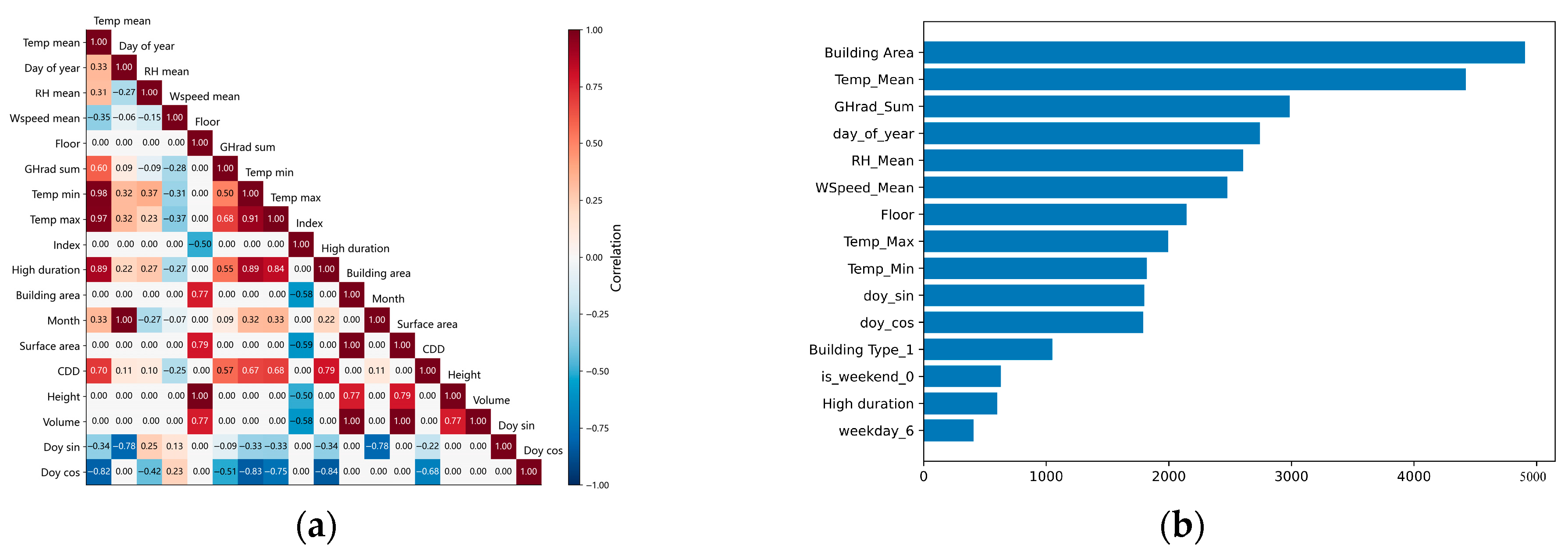
Figure A2.
Schematic diagram of time-block data splitting. The arrow indicates the chronological order of the samples along the horizontal axis, representing days 1 to 365 within a year.
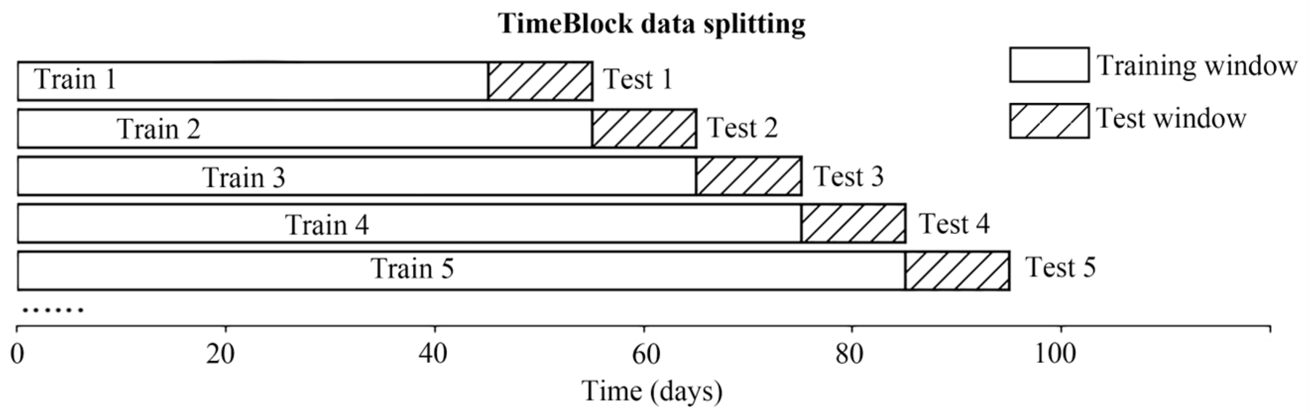
Figure A3.
Man-made disruption to the daily routine.
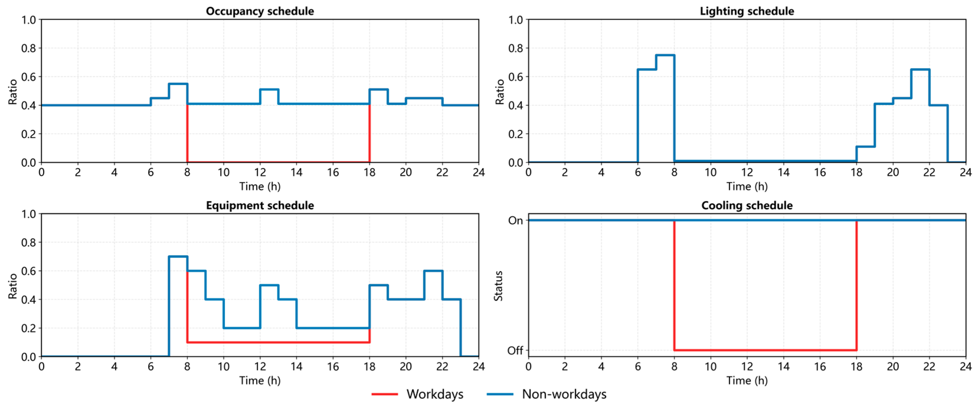
Table A2.
Detailed parameter settings for each building.
References
- China Association of Building Energy Efficiency, Building Energy and Carbon Emissions Data Committee. Research Report on Carbon Emissions in the Field of Urban and Rural Development in China (2024 Edition); China Association of Building Energy Efficiency: Chongqing, China, 2024. [Google Scholar]
- Tao, S.; Ru, M.Y.; Du, W.; Zhu, X.; Zhong, Q.R.; Li, B.G.; Shen, G.F.; Pan, X.L.; Meng, W.J.; Chen, Y.L.; et al. Quantifying the Rural Residential Energy Transition in China from 1992 to 2012 through a Representative National Survey. Nat. Energy 2018, 3, 567–573. [Google Scholar] [CrossRef] [Scilit]
- Huo, T.; Ma, Y.; Cai, W.; Liu, B.; Mu, L. Will the Urbanization Process Influence the Peak of Carbon Emissions in the Building Sector? A Dynamic Scenario Simulation. Energy Build. 2021, 232, 110590. [Google Scholar] [CrossRef] [Scilit]
- Fenner, A.E.; Kibert, C.J.; Woo, J.; Morque, S.; Razkenari, M.; Hakim, H.; Lu, X. The Carbon Footprint of Buildings: A Review of Methodologies and Applications. Renew. Sustain. Energy Rev. 2018, 94, 1142–1152. [Google Scholar] [CrossRef] [Scilit]
- Liu, Z.; Wang, F.; Tang, Z.; Tang, J. Predictions and Driving Factors of Production-Based CO2 Emissions in Beijing, China. Sustain. Cities Soc. 2020, 53, 101909. [Google Scholar] [CrossRef] [Scilit]
- Chen, B.; Chen, F.; Ciais, P.; Zhang, H.; Lü, H.; Wang, T.; Chevallier, F.; Liu, Z.; Yuan, W.; Peters, W. Challenges to Achieve Carbon Neutrality of China by 2060: Status and Perspectives. Sci. Bull. 2022, 67, 2030–2035. [Google Scholar] [CrossRef] [Scilit]
- Li, X.; Lin, C.; Lin, M.; Jim, C.Y. Drivers and Spatial Patterns of Carbon Emissions from Residential Buildings: An Empirical Analysis of Fuzhou City (China). Build. Environ. 2024, 257, 111534. [Google Scholar] [CrossRef] [Scilit]
- Sheng, Y.; Arbabi, H.; Ward, W.O.C.; Alvarez, M.A.; Mayfield, M. City-Scale Residential Energy Consumption Prediction with a Multimodal Approach. Sci. Rep. 2025, 15, 5313. [Google Scholar] [CrossRef] [Scilit]
- Gao, J.; Liu, H.; Tang, Y.; Luo, M. Hybrid Method of Mapping Urban Residential Carbon Emissions with High-Spatial Resolution: A Case Study of Suzhou, China. Environ. Plan. B Urban Anal. City Sci. 2024, 51, 75–88. [Google Scholar] [CrossRef] [Scilit]
- Song, C.; Deng, Z.; Zhao, W.; Yuan, Y.; Liu, M.; Xu, S.; Chen, Y. Developing Urban Building Energy Models for Shanghai City with Multi-Source Open Data. Sustain. Cities Soc. 2024, 106, 105425. [Google Scholar] [CrossRef] [Scilit]
- Ramos, P.V.B.; Villela, S.M.; Silva, W.N.; Dias, B.H. Residential Energy Consumption Forecasting Using Deep Learning Models. Appl. Energy 2023, 350, 121705. [Google Scholar] [CrossRef] [Scilit]
- Intergovernmental Panel on Climate Change. IPCC Climate Change 2023: Synthesis Report; Core Writing Team, Lee, H., Romero, J., Eds.; Contribution of Working Groups I, II and III to the Sixth Assessment Report of the Intergovernmental Panel on Climate Change; IPCC: Geneva, Switzerland, 2023; p. 184. [Google Scholar]
- Muntean, M.; Janssens-Maenhout, G.; Song, S.; Giang, A.; Selin, N.E.; Zhong, H.; Zhao, Y.; Olivier, J.G.J.; Guizzardi, D.; Crippa, M.; et al. Evaluating EDGARv4.Tox2 Speciated Mercury Emissions Ex-Post Scenarios and Their Impacts on Modelled Global and Regional Wet Deposition Patterns. Atmos. Environ. 2018, 184, 56–68. [Google Scholar] [CrossRef] [Scilit]
- Oda, T.; Maksyutov, S.; Andres, R.J. The Open-Source Data Inventory for Anthropogenic CO2, Version 2016 (ODIAC2016): A Global Monthly Fossil Fuel CO2 Gridded Emissions Data Product for Tracer Transport Simulations and Surface Flux Inversions. Earth Syst. Sci. Data 2018, 10, 87–107. [Google Scholar] [CrossRef] [Scilit]
- Chen, S.; Li, N.; Guan, J.; Xie, Y.; Sun, F.; Ni, J. A Statistical Method to Investigate National Energy Consumption in the Residential Building Sector of China. Energy Build. 2008, 40, 654–665. [Google Scholar] [CrossRef] [Scilit]
- Cui, X.; Lee, M.; Koo, C.; Hong, T. Energy Consumption Prediction and Household Feature Analysis for Different Residential Building Types Using Machine Learning and SHAP: Toward Energy-Efficient Buildings. Energy Build. 2024, 309, 113997. [Google Scholar] [CrossRef] [Scilit]
- Zheng, L.; Luo, K.; Zhao, L. An Operational Carbon Emission Prediction Model Based on Machine Learning Methods for Urban Residential Buildings in Guangzhou. Buildings 2024, 14, 3699. [Google Scholar] [CrossRef] [Scilit]
- Huang, R.; Zhang, X.; Liu, K. Assessment of Operational Carbon Emissions for Residential Buildings Comparing Different Machine Learning Approaches: A Study of 34 Cities in China. Build. Environ. 2024, 250, 111176. [Google Scholar] [CrossRef] [Scilit]
- Zhu, X.X.; Chen, S.; Zhang, F.; Shi, Y.; Wang, Y. Global Building Atlas: An Open Global and Complete Dataset of Building Polygons, Heights and LoD1 3D Models. Earth Syst. Sci. Data 2025, 17, 6647–6668. [Google Scholar] [CrossRef] [Scilit]
- Wu, W.-B.; Ma, J.; Banzhaf, E.; Meadows, M.E.; Yu, Z.-W.; Guo, F.-X.; Sengupta, D.; Cai, X.-X.; Zhao, B. A First Chinese Building Height Estimate at 10 m Resolution (CNBH-10 m) Using Multi-Source Earth Observations and Machine Learning. Remote Sens. Environ. 2023, 291, 113578. [Google Scholar] [CrossRef] [Scilit]
- Lundberg, S.M.; Lee, S.-I. A Unified Approach to Interpreting Model Predictions. In Proceedings of the Advances in Neural Information Processing Systems 30 (NIPS 2017); Guyon, I., Luxburg, U.V., Bengio, S., Wallach, H., Fergus, R., Vishwanathan, S., Garnett, R., Eds.; Neural Information Processing Systems (NIPS): Long Beach, CA, USA, 2017; Volume 30. [Google Scholar]
- Li, J.; Yu, Z.; Haghighat, F.; Zhang, G. Development and Improvement of Occupant Behavior Models towards Realistic Building Performance Simulation: A Review. Sustain. Cities Soc. 2019, 50, 101685. [Google Scholar] [CrossRef] [Scilit]
- Peng, Y.; Rysanek, A.; Nagy, Z.; Schlüter, A. Using Machine Learning Techniques for Occupancy-Prediction-Based Cooling Control in Office Buildings. Appl. Energy 2018, 211, 1343–1358. [Google Scholar] [CrossRef] [Scilit]
- Liang, X.; Hong, T.; Shen, G.Q. Improving the Accuracy of Energy Baseline Models for Commercial Buildings with Occupancy Data. Appl. Energy 2016, 179, 247–260. [Google Scholar] [CrossRef] [Scilit]
- Liu, G.; Zheng, Y.; Xu, X.; Liu, X.; Zhang, H.; Ou, J. Fine-Scale Estimation of Building Operation Carbon Emissions: A Case Study of the Pearl River Delta Urban Agglomeration. Build. Simul. 2025, 18, 957–977. [Google Scholar] [CrossRef] [Scilit]
- Tao, M.; Cai, Z.; Che, K.; Liu, Y.; Yang, D.; Wu, L.; Wang, P.; Yang, M. Cross-Inventory Uncertainty Analysis of Fossil Fuel CO2 Emissions for Prefecture-Level Cities in Shandong Province. Atmosphere 2022, 13, 1474. [Google Scholar] [CrossRef] [Scilit]
- Super, I.; Dellaert, S.N.C.; Visschedijk, A.J.H.; Denier Van Der Gon, H.A.C. Uncertainty Analysis of a European High-Resolution Emission Inventory of CO2 and CO to Support Inverse Modelling and Network Design. Atmos. Chem. Phys. 2020, 20, 1795–1816. [Google Scholar] [CrossRef] [Scilit]
- Wang, G.; Hu, Q.; He, L.; Guo, J.; Huang, J.; Zhong, L. The Estimation of Building Carbon Emission Using Nighttime Light Images: A Comparative Study at Various Spatial Scales. Sustain. Cities Soc. 2024, 101, 105066. [Google Scholar] [CrossRef] [Scilit]
- Zhao, B.; Deng, M.; Lo, S.; Liu, B. Estimating Built-up Area Carbon Emissions through Addressing Regional Development Disparities with Population and Nighttime Light Data. Appl. Energy 2024, 369, 123582. [Google Scholar] [CrossRef] [Scilit]
- Yin, Z.; Chen, F.; Dou, C.; Wu, M.; Niu, Z.; Wang, L.; Xu, S. Identification of Illumination Source Types Using Nighttime Light Images from SDGSAT-1. Int. J. Digit. Earth 2024, 17, 2297013. [Google Scholar] [CrossRef] [Scilit]
- Fong, W.; Sun, Y.; Chen, Y. Examining the Relationship between Energy Consumption and Unfavorable CO2 Emissions on Sustainable Development by Going through Various Violated Factors and Stochastic Disturbance–Based on a Three-Stage SBM-DEA Model. Energies 2022, 15, 569. [Google Scholar] [CrossRef] [Scilit]
- Zhang, Y.; Sun, T.; Wang, L.; Huang, B.; Xu, S.; Pan, X.; Xiong, X.; Song, W.; Li, G.; Niu, Z. Integrating Panoptic-AI and Multi-Source Observations for Daytime Dynamic CO2 Increment Prediction in Urban Traffic Networks. Sustain. Cities Soc. 2025, 131, 106730. [Google Scholar] [CrossRef] [Scilit]
- Xu, P.; Huang, J.; Shen, P.; Ma, X.; Gao, X.; Xu, Q.; Jiang, H.; Xiang, Y. Commercial Building Energy Use in Six Cities in Southern China. Energy Policy 2013, 53, 76–89. [Google Scholar] [CrossRef] [Scilit]
- Reinhart, C.F.; Cerezo Davila, C. Urban Building Energy Modeling—A Review of a Nascent Field. Build. Environ. 2016, 97, 196–202. [Google Scholar] [CrossRef] [Scilit]
- Khalil, M.; McGough, A.S.; Pourmirza, Z.; Pazhoohesh, M.; Walker, S. Machine Learning, Deep Learning and Statistical Analysis for Forecasting Building Energy Consumption—A Systematic Review. Eng. Appl. Artif. Intell. 2022, 115, 105287. [Google Scholar] [CrossRef] [Scilit]
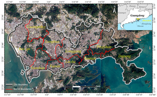
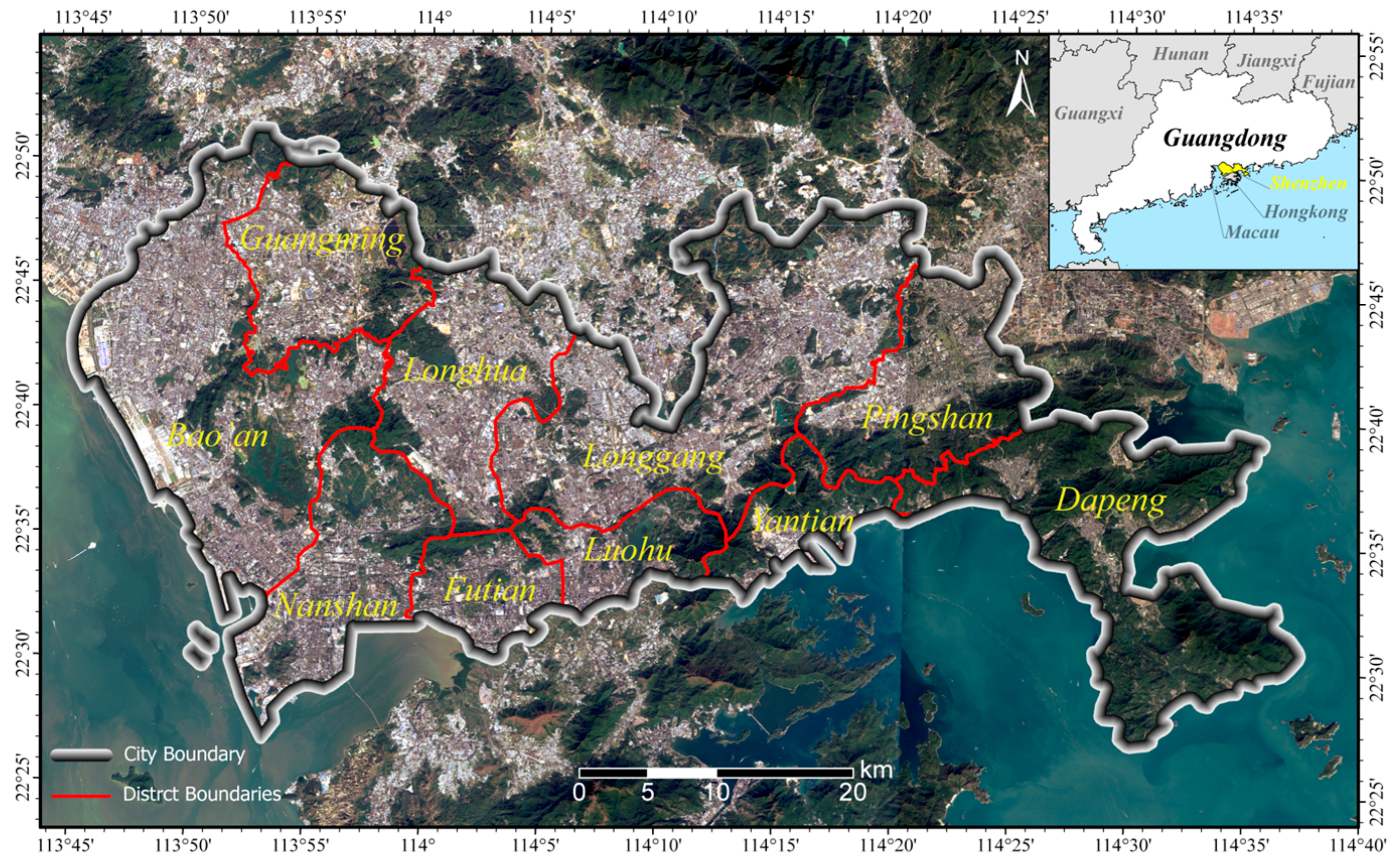
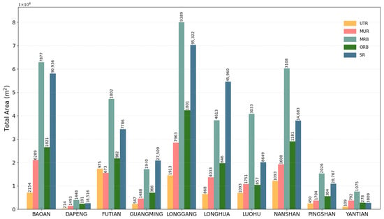
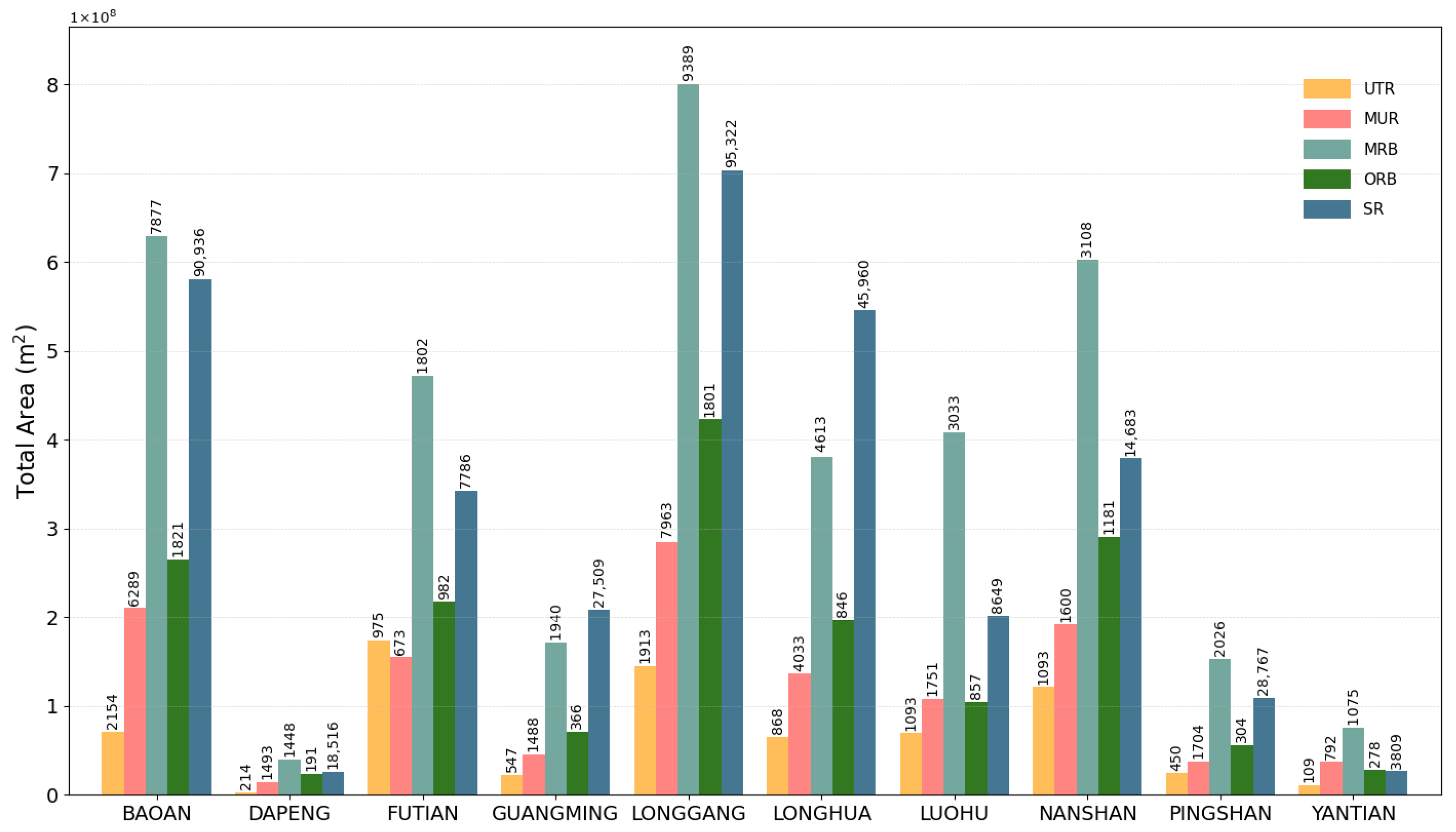
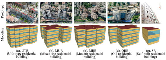
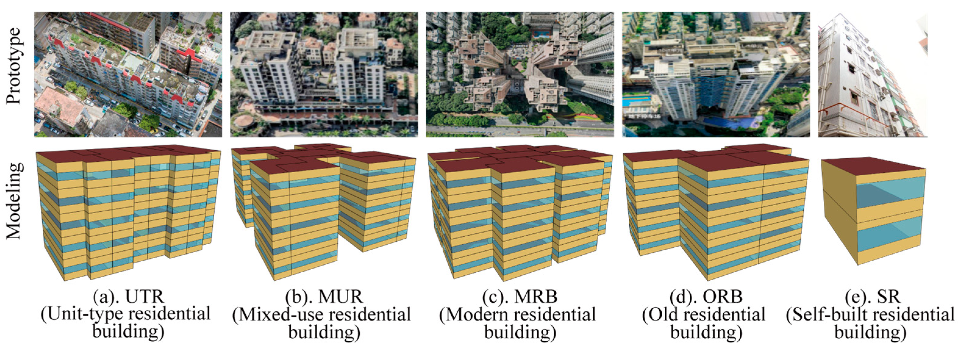
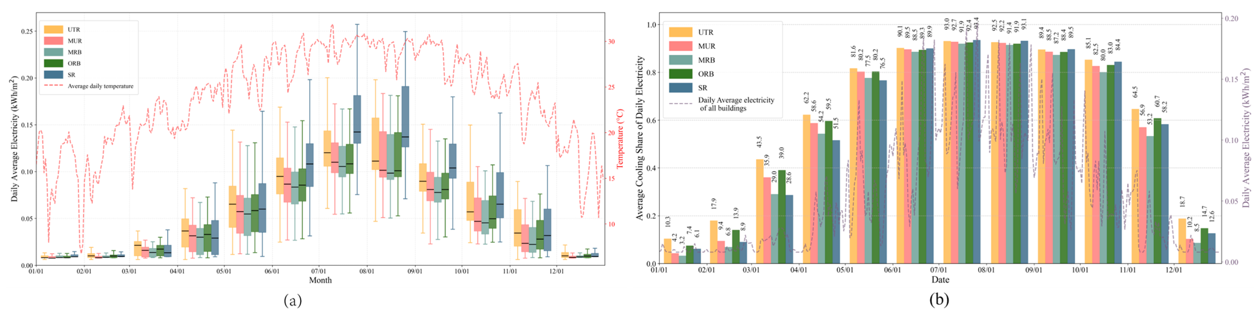
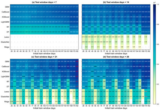
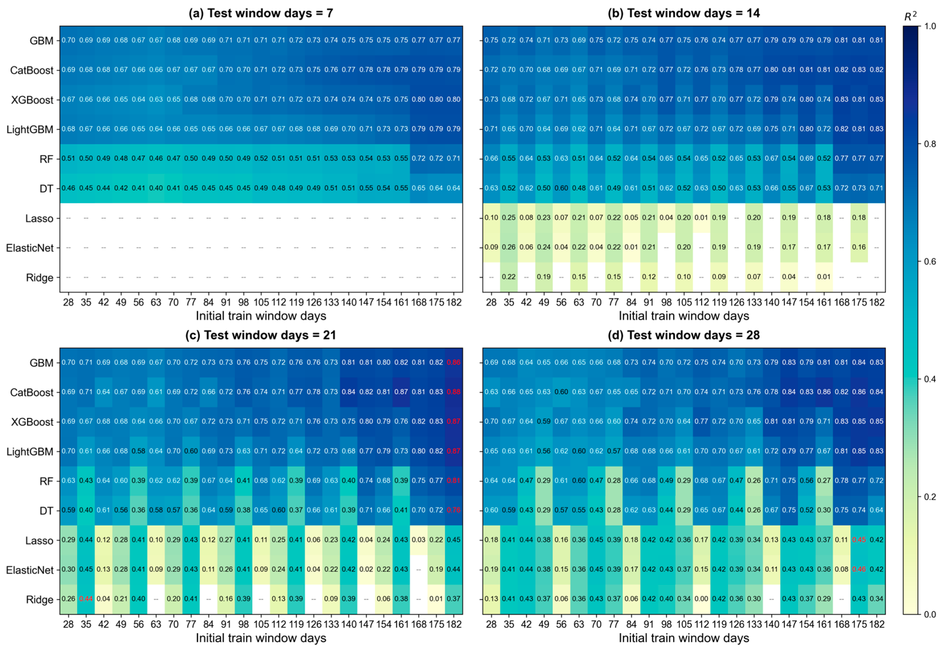
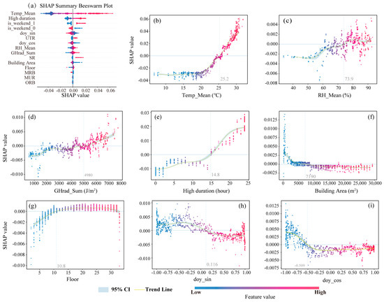
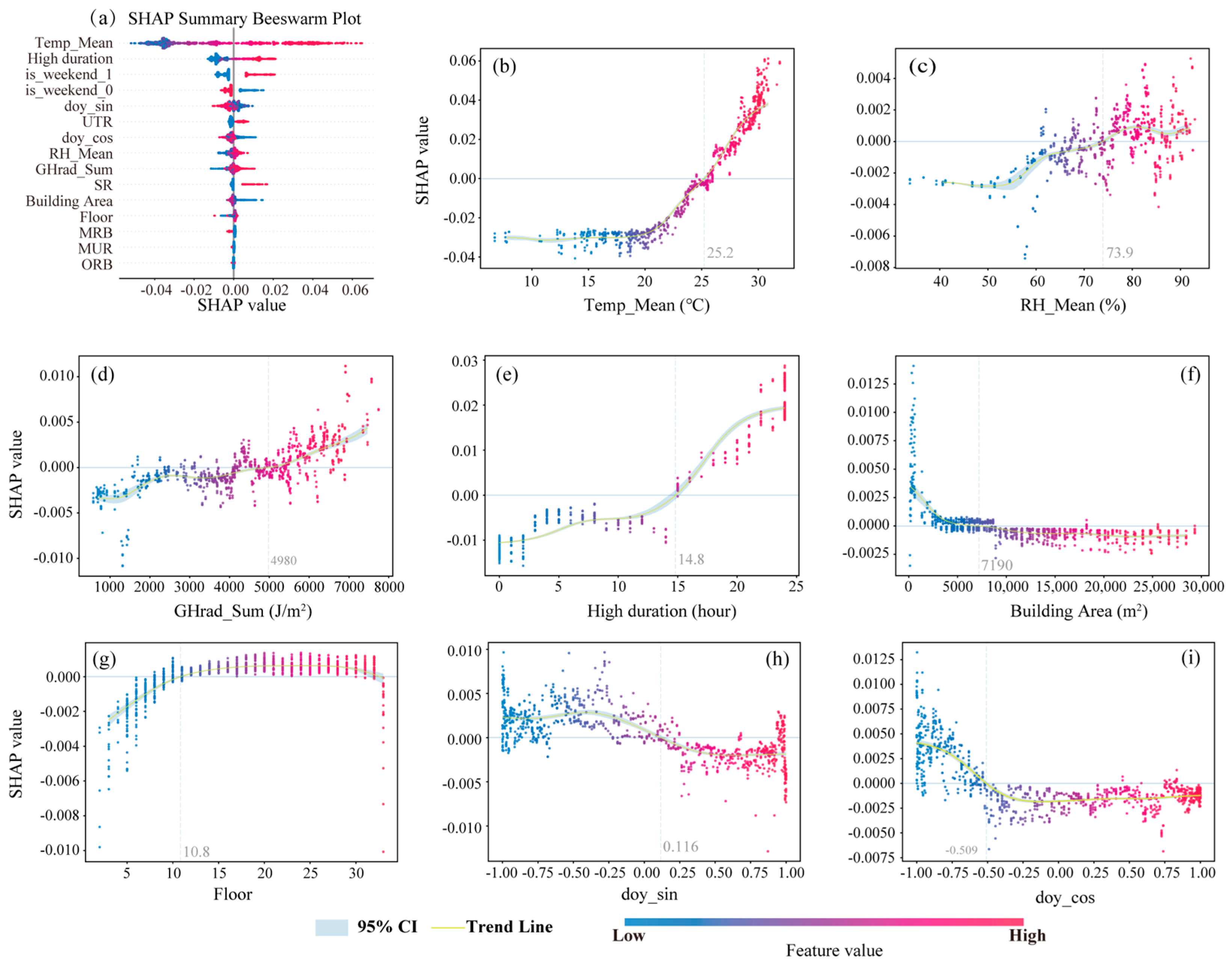
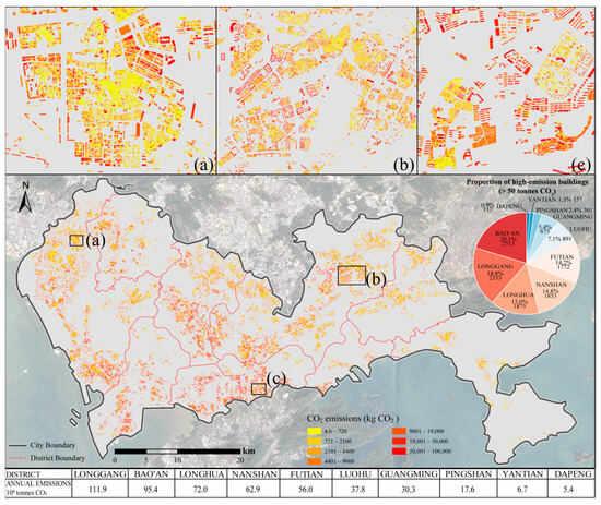
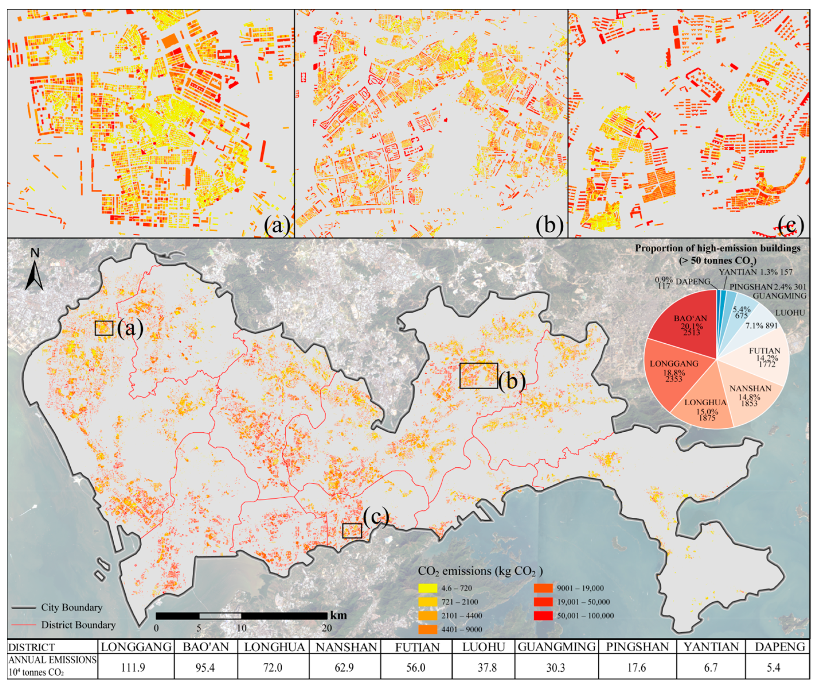
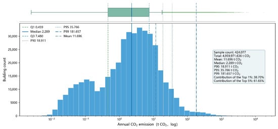
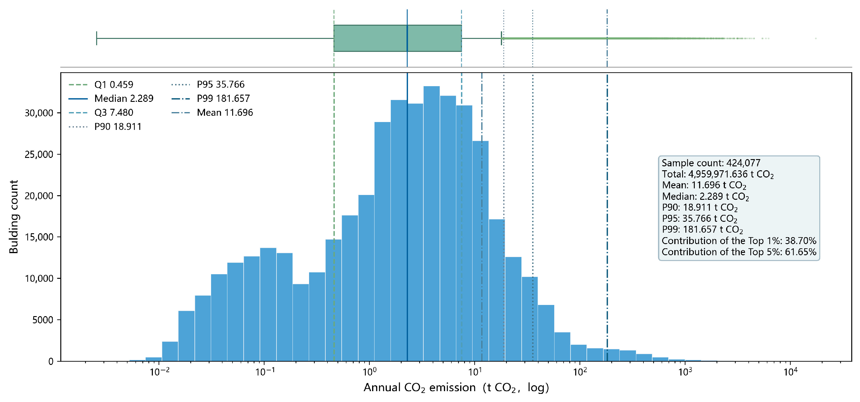
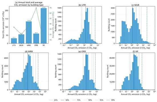
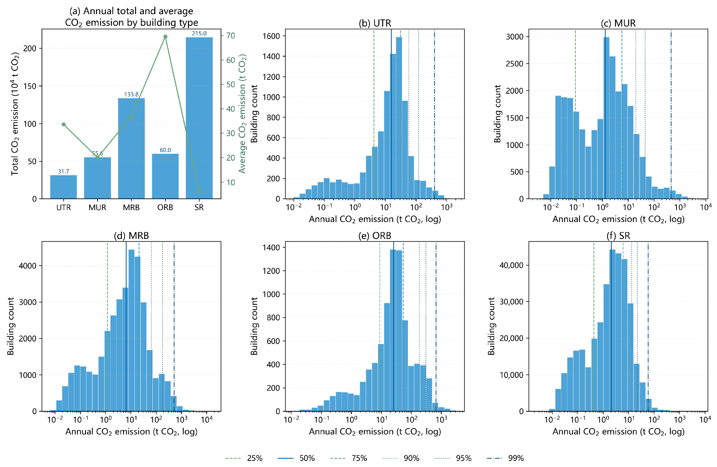
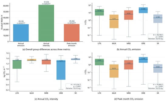
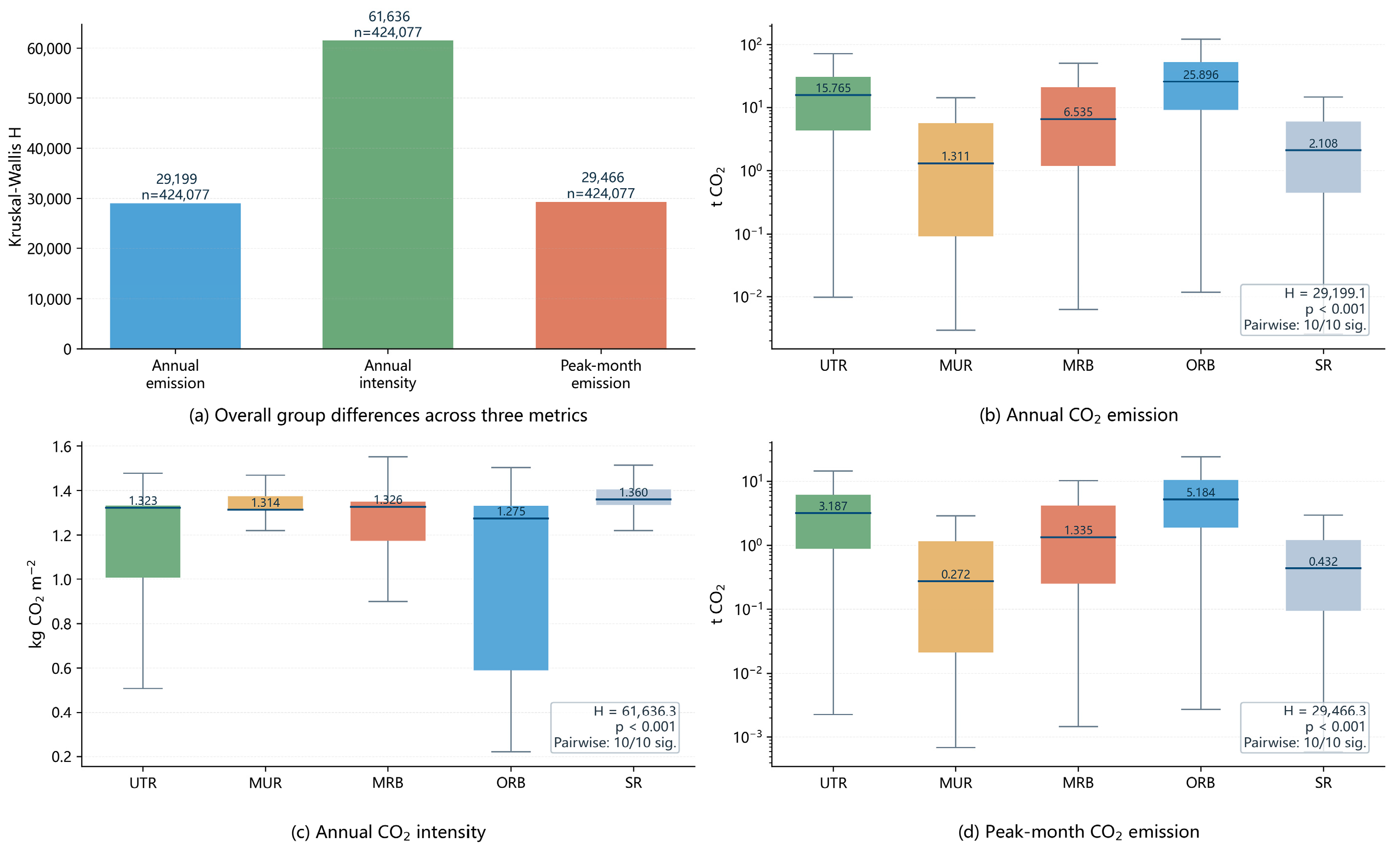
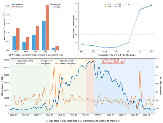
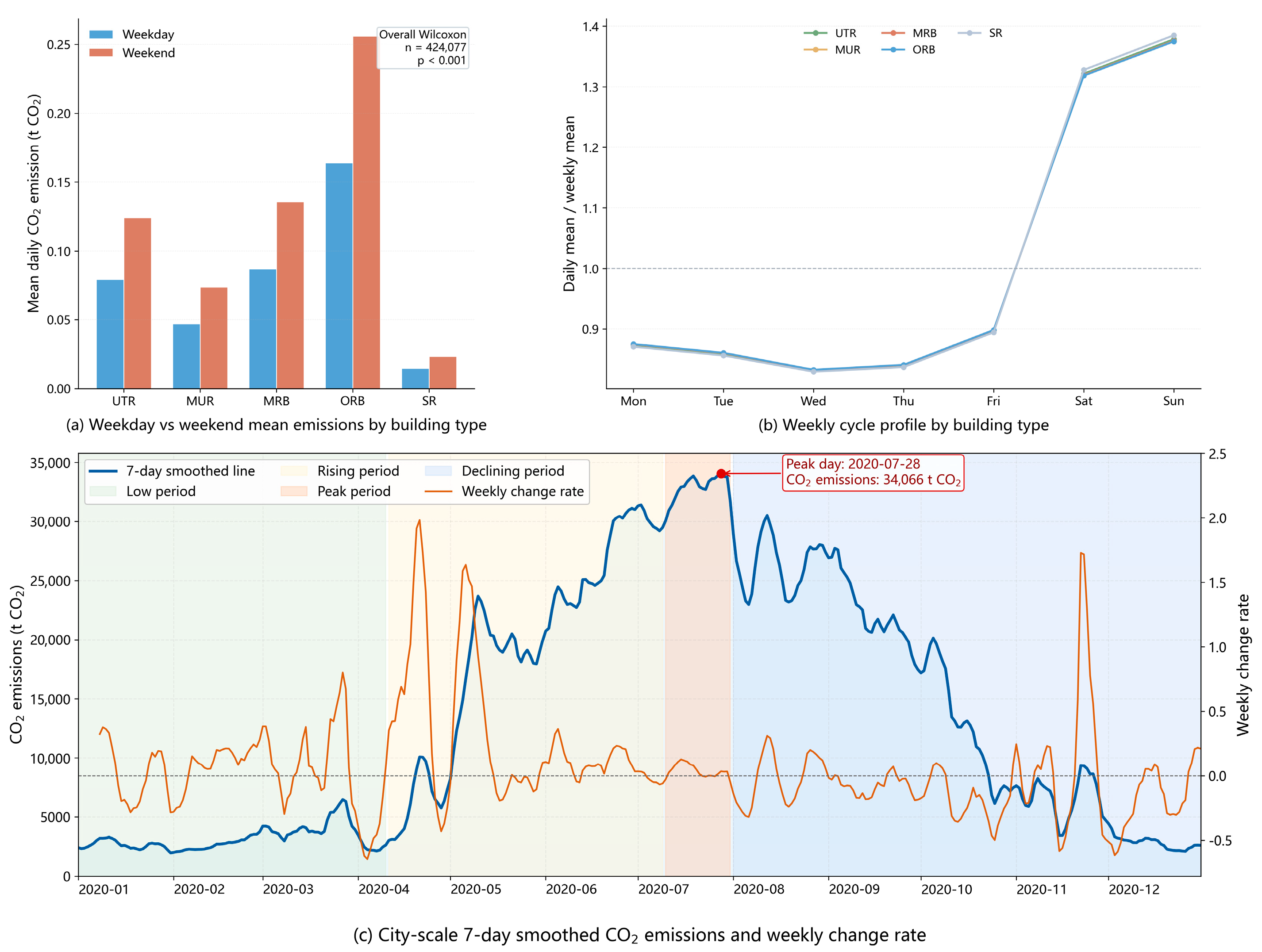
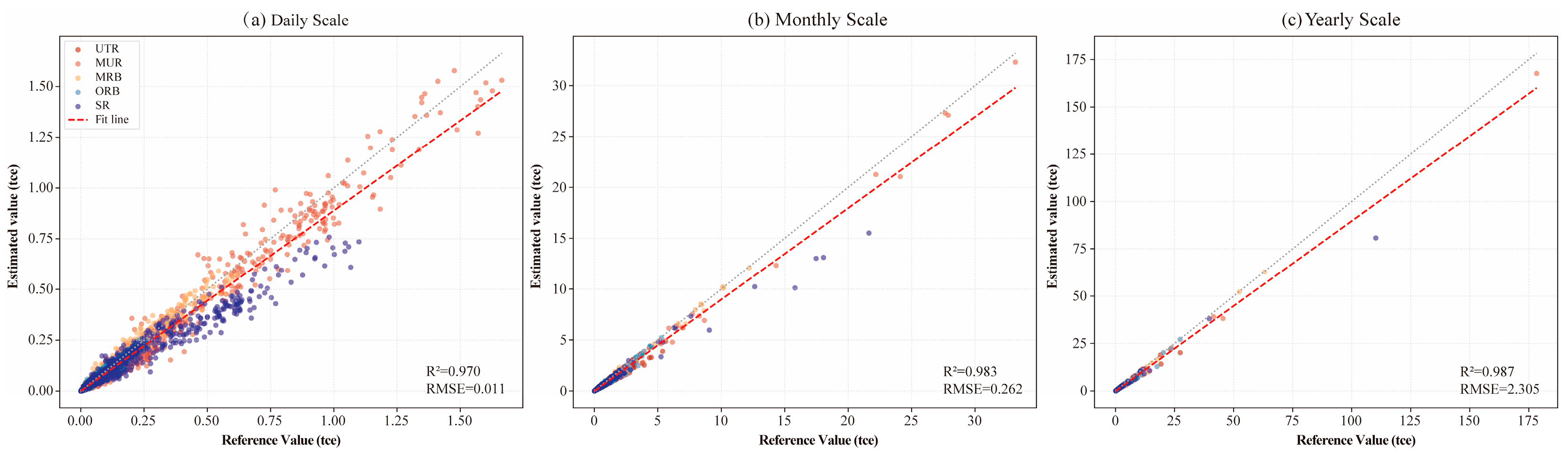
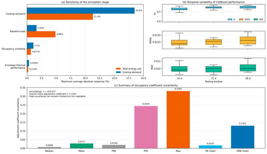
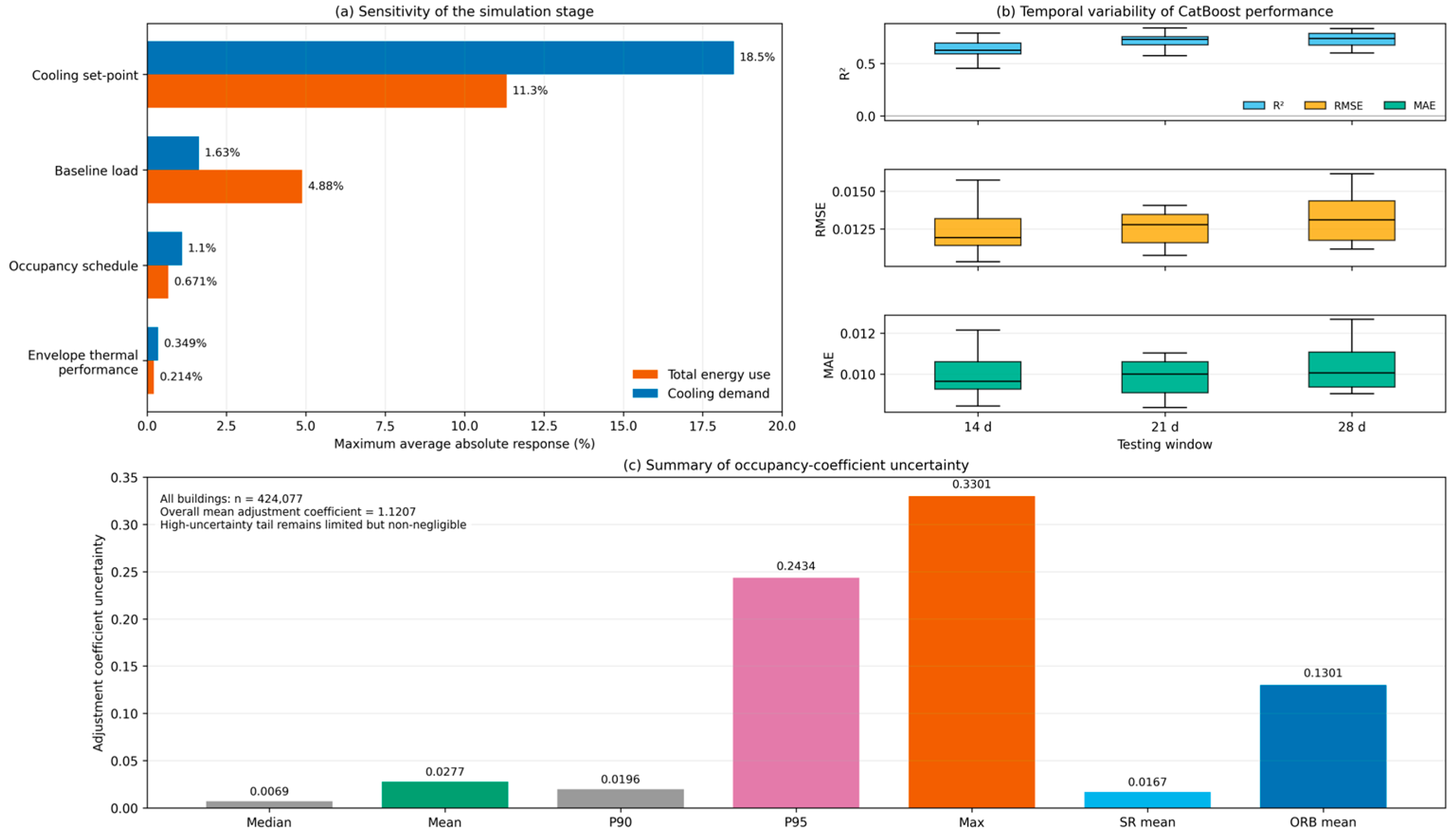
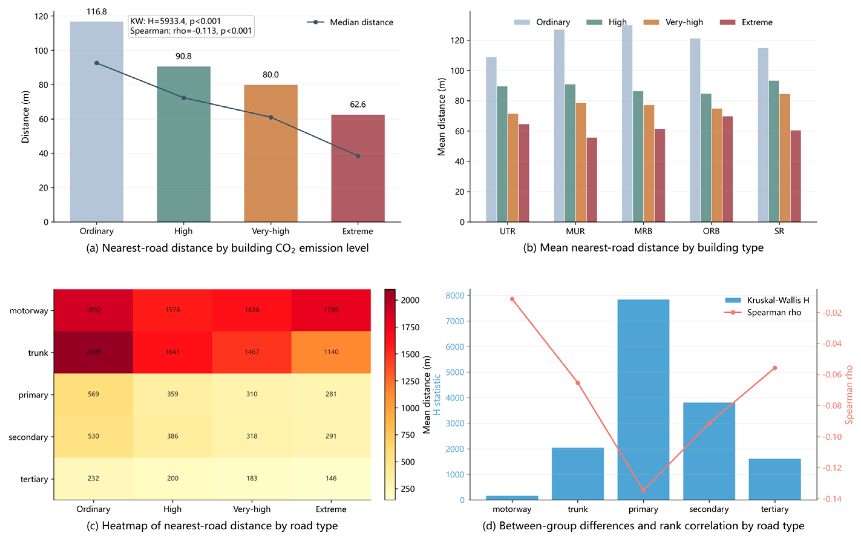

Disclaimer/Publisher’s Note: The statements, opinions and data contained in all publications are solely those of the individual author(s) and contributor(s) and not of MDPI and/or the editor(s). MDPI and/or the editor(s) disclaim responsibility for any injury to people or property resulting from any ideas, methods, instructions or products referred to in the content. |
© 2026 by the authors. Licensee MDPI, Basel, Switzerland. This article is an open access article distributed under the terms and conditions of the Creative Commons Attribution (CC BY) license.