Coupling Effects of Land Use Carbon Emissions and Ecological Security in Border Cities of Jilin Province, China

Abstract

Rapid urbanization has led to a significant increase in land use carbon emission (LCE), putting great pressure on ecological security. The coupling relationship between LCE and the ecological security index (ESI) is the key to sustainable development. Based on land use/cover change (LUCC) and Open-Data Inventory for Anthropogenic Carbon dioxide (ODIAC) data, the LCE of the Jilin Border Cities (JLBCs) from 2013 to 2023 was estimated. Twenty-seven indicators were selected from both natural and socioeconomic aspects to evaluate the ESI using the Driving forces–Pressure–State–Impact–Response–Management (DPSIRM) model. The spatial interaction between LCE and ESI was analyzed using the coupling degree model and spatial autocorrelation. The results show that from 2013 to 2023, the main LCE areas in the JLBCs were concentrated in central urban districts, while the total LCE remained negative but exhibited a clear upward trend. The ESIs in Tonghua City and Baishan City have continued to improve, but those in Yanbian Autonomous Prefecture have gradually deteriorated, with ecological security warnings intensifying progressively toward the east. The spatial variation in the LCE–ESI coupling degree is significant, predominantly exhibiting low coupling with differences across scales. Within the study area, coupling degree shows a strong positive correlation, revealing distinct spatial clustering patterns dominated by low clusters and cold spots. Future efforts should focus on promoting low-carbon development models, strengthening protection and restoration, while implementing targeted measures to enhance the overall ecology of JLBCs.

1. Introduction

In the wave of globalization, sustainable development faces the dual impact of urban expansion and environmental pressure [1,2,3]. While urbanization promotes economic growth and social progress, it also triggers drastic changes in land use patterns, posing a severe threat to ecological security [4]. As a critical component of the global carbon cycle, research on land use carbon emission (LCE) has gradually become a core area in addressing climate change [4]. Land use/cover change (LUCC) driven by human activities generates substantial LCE, accounting for one-third of total direct carbon emissions [5,6]. This disrupts the terrestrial carbon balance [7] and leads to a decline in the ecological security index (ESI) [8]. Therefore, exploring the interrelationship between urban development and ecological security is crucial for sustainable urban development.

Extensive research has been conducted to estimate LCE using diverse methodologies. Among these, the carbon emission factor method has emerged as the predominant approach [9,10]. Derived from IPCC guidelines, this method accounts not only for direct carbon emissions generated by different LUCCs but also incorporates indirect carbon emissions from human fossil fuel use [7,11] and offers a relatively convenient calculation process [9]. However, most studies rely on energy consumption statistical data to calculate direct carbon emissions, which restricts them to large-scale administrative units [4,5,10] and makes it difficult to adequately reflect micro-scale characteristics. Case studies focusing on border cities are particularly scarce. Recently, Yang and Li (2022) proposed a new LCE estimation method that combines LUCC with ODIAC data, enabling research at the meter scale [11]. ODIAC data, with higher resolution than statistical data, have been widely applied in various studies [12,13].

With population growth, China’s rapid socioeconomic development is impacting the ecological environment and disrupting the ecological balance [14,15]. Ecological security refers to the state in which natural and semi-natural ecosystems maintain and safeguard the sustainable development of human society without being damaged or threatened, reflecting the integrity and health of ecosystems at the holistic level [16]. In recent years, significant progress has been made in evaluation methods and indicator construction, with a shift from single ecosystem indicators to optimized multi-dimensional indicator systems [17]. Current evaluation methods are largely model-based, and the Pressure–State–Response (PSR) model is one of the most widely used approaches in ecological security research [18]. However, the PSR model has a notable limitation: it can only indirectly reflect the impact of human activities on the environment through temporal changes in environmental state indicators. Meanwhile, current ecological security evaluation systems remain limited in addressing the dynamics and complexity of specific evaluation subjects, and a systematic framework for applied research on border cities has yet to be established. Consequently, this study employs an enhanced PSR model—the Driving forces–Pressure–State–Impact–Response–Management (DPSIRM) model—to assess urban ecological security [19,20]. This model not only significantly advances traditional qualitative research approaches in the field of urban ecological security evaluation but also provides robust support for urban ecological environment management and sustainable development.

Studies have found that LCE and the ESI influence each other to some extent [6,21], exhibiting a profound coupling relationship. When LCE is generated, LUCC alters ecosystem structure, processes, and functions [4] and disrupts landscape patterns [22], negatively affecting ecological security by changing land use types and ecosystem functions [15]. Conversely, a favorable ecological security status can provide sufficient ecosystem products, enhance carbon sink functions, and alleviate the pressure of LCE [23]. Existing studies have mostly explored the relationship between the two from a unidirectional perspective, with few focusing on their coupling relationship, leaving the mutual influence mechanisms unelucidated. As an important part of the national ecological security barrier, the coupling relationship between LCE and the ESI in border cities is unique [24]. Border cities typically face multiple contradictions [25], as their distinct geopolitical, economic, and ecological characteristics necessitate specialized policies and technologies to address climate change and achieve sustainable development. However, systematic research on the coupling effects of LCE and the ESI in border cities remains limited [26].

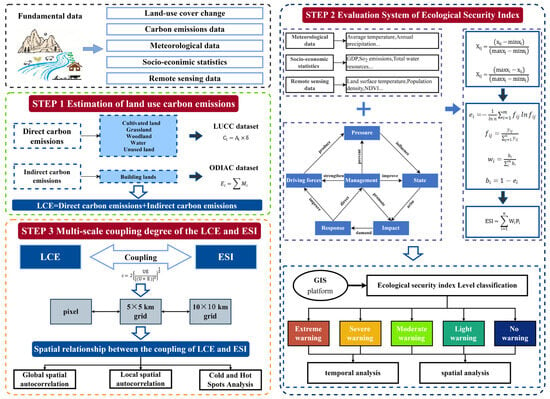
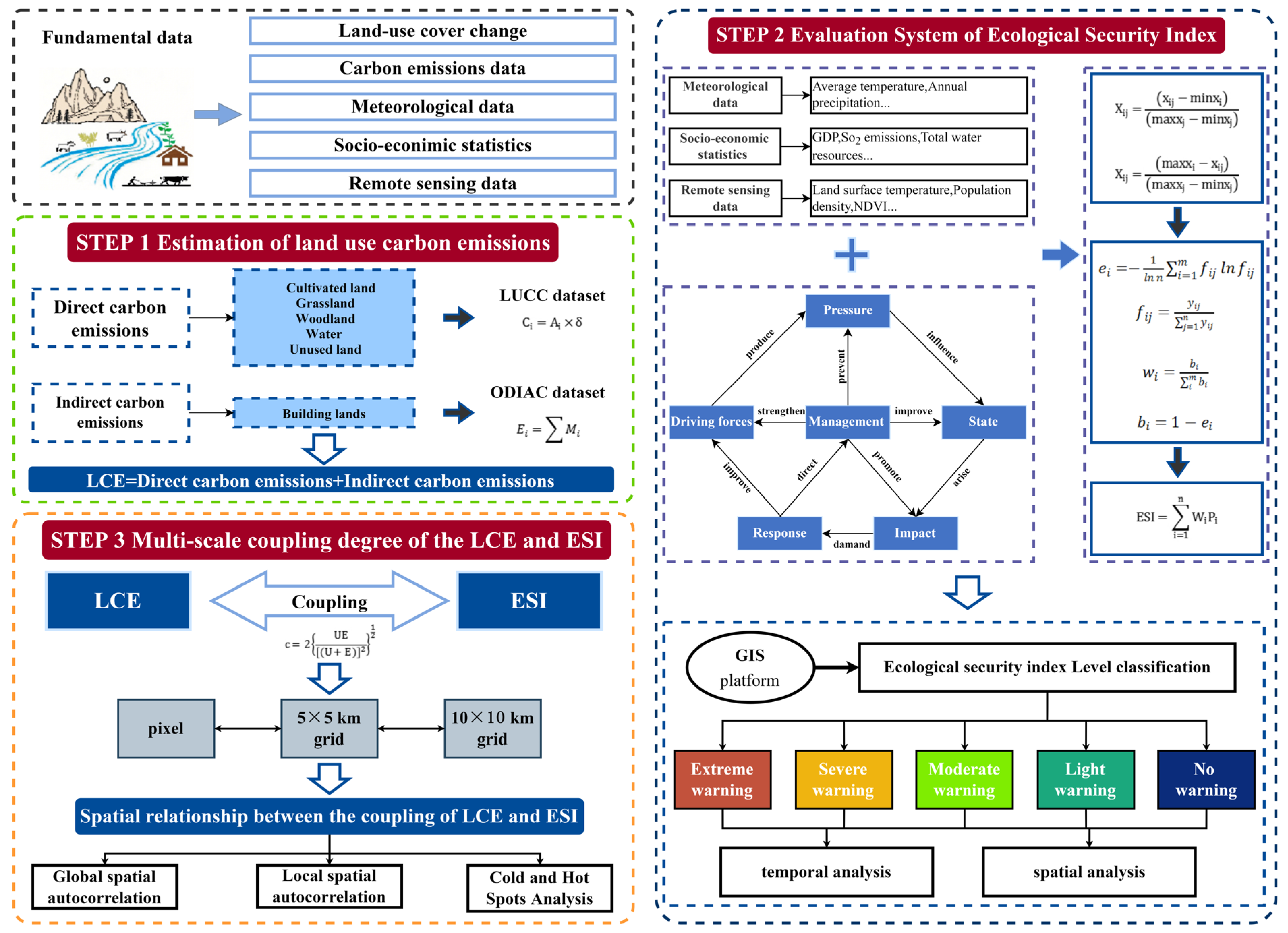
This study focuses on JLBCs. Using LUCC data and ODIAC data, it estimates LCE of JLBCs from 2013 to 2023. The 27 indicators selected from natural and socioeconomic dimensions are applied to conduct a comprehensive evaluation of the ESI for JLBCs from 2013 to 2023 using the DPSIRM model. The coupling degree model and spatial analysis methods are employed to analyze the spatial interactions between LCE and the ESI (as shown in Figure 1). This study focuses on border cities as a unique region, delving into the spatiotemporal evolution characteristics and coupling relationships between LCE and the ESI. It provides theoretical foundations and decision support for the sustainable development of border cities while addressing gaps in current research on these areas.

Figure 1. Research framework.

2. Study Area and Data Sources

2.1. Study Area

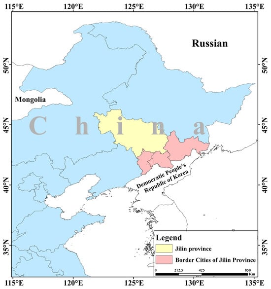
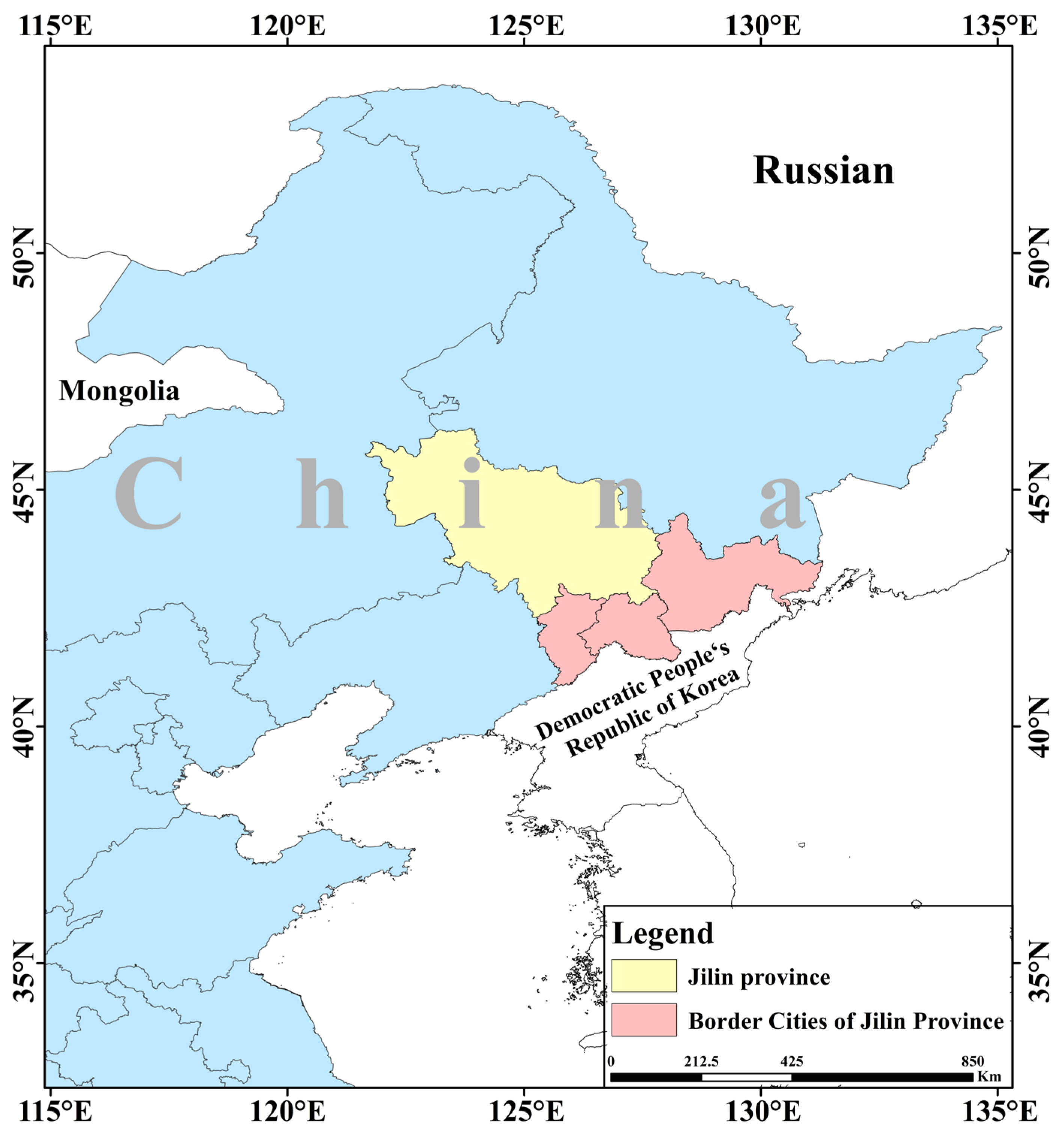
The Jilin Border Cities (JLBCs) region is situated between 125° E~132° E and 40° N~50° N, bordering the Democratic People’s Republic of Korea and the Russian Federation (as shown in Figure 2). This region comprises 3 prefecture-level cities (Tonghua City, Baishan City, and Yanbian Korean Autonomous Prefecture) and 20 counties and cities, covering a total area of approximately 76,700 km². It accounts for 40.07% of Jilin Province’s total area and 17.6% of its population. Numerous rivers and lakes crisscross the region, providing a solid ecological foundation while also serving dual functions as boundary rivers and transportation waterways. Located in the Changbai Mountain, this region boasts exceptionally rich forest, mineral, and flora and fauna resources. The JLBCs region has various border ports, including road, rail, and air transport, serving as a vital gateway for opening up to the outside world. However, the JLBCs still face numerous challenges. For instance, their industrial structures are overly reliant on resource-based and traditional industries, leading to issues such as poor sustainability and low-quality urbanization. Consequently, the economic growth rate in the northeastern border region lags significantly behind the national average for border cities. This places higher demands on its infrastructure conditions and social governance capabilities. Within this environment, exploring the coordinated development of LCE and the ESI is of paramount importance.

Figure 2. Location map of JLBCs.

2.2. Data Sources

2.2.1. Ecological Security Data

Based on the DPSIRM model, combined with the actual situation and relevant research of JLBCs, this study selects 27 indicators from 6 perspectives: driving factors, pressure, state, impact, response, and management of border city ecological security, to construct an evaluation index system for border city ecological security, as shown in Table 1. This study adopts a method combining statistical data and remote sensing data indicators to assess the ecological security of border cities at the regional scale. These indicators are divided into 3 categories: meteorological data (2 in total), mainly sourced from the National Tibetan Plateau Scientific Data Center, socioeconomic statistical indicators (18 in total) from sources such as the “Jilin Statistical Yearbook 2014–2025”, “Statistical Communique on the National Economic and Social Development of the People’s Republic of China”, “China City Statistical Yearbook”, and “China County Statistical Yearbook”, and remote sensing data indicators (6 in total) from the China Multitemporal Land Use and Cover Change Monitoring Dataset (CNLUCC) with a spatial resolution of 30 m, as well as MODIS product data. Land use data follow national standards, dividing land use/cover types into six major categories for indicator calculation and land use analysis. Other indicators are calculated by extracting source data.

Table 1. Ecological security evaluation indicator system.

Objective Layer	Guideline Layer	Indicator Layer	Attribute	Data Attributes
ESI of JLBCs	Driving force	Average temperature/°	−	Meteorological data
		Annual precipitation/mm	+	Meteorological data
		GDP/10,000 people	+	Statistical data
		Per capita GDP/RMB 1	+	Statistical data
		Natural population growth rate/%	−	Statistical data
	Pressure	Population density/people·(km2)−1	−	Remote sensing data
		Building land occupation	−	Extracting data
		NPP-VIIRS Night light data/(nW/cm2/sr)	−	Remote sensing data
		Number of industrial enterprises above scale	−	Statistical data
		SO2 emissions/ton	−	Statistical data
	State	NDVI	+	Remote sensing data
		Net primary productivity of vegetation/gC·(m2·a)−1	+	Remote sensing data
		Total water resources/cubic meter	+	Statistical data
		Number of foreign-invested enterprises	+	Statistical data
		International tourism arrivals/person	+	Statistical data
	Impact	Primary sector workers/10,000 people	+	Statistical data
		Value of goods exported/RMB 10,000	+	Statistical data
		Value of goods imported/RMB 10,000	+	Statistical data
		Potential evapotranspiration/kg·(m2)−1	−	Remote sensing data
		Land surface temperature/°	−	Remote sensing data
	Response	Percentage of tertiary sector/%	+	Statistical data
		Green space coverage of built-up areas/%	+	Statistical data
		Landscaped area/hm2	+	Statistical data
		International tourism revenues/USD 10,000	+	Statistical data
	Management	Fiscal expenditure on education/RMB 10,000	+	Statistical data
		Fiscal expenditure on science/RMB 10,000	+	Statistical data
		Centralized wastewater treatment plant rate/%	+	Statistical data

2.2.2. Carbon Emissions Data

The ODIAC dataset was used to calculate carbon emissions from construction land. ODIAC is a data product of global CO₂ emissions from fossil fuel combustion reflecting carbon emissions from human activities [27]. ODIAC data from the Centre for Global Environmental Studies (https://db.cger.nies.go.jp/) is a gridded dataset of global CO₂ emissions produced by the National Institute for Environmental Studies through the Greenhouse Gas Observing Satellite project [28]. ODIAC is the first organization to identify the global spatial extent of fossil fuel CO₂ emissions by combining nighttime light data with individual power plant emission and location profiles [29]. ODIAC uses an innovative emissions modeling approach to obtain a fine-grained image of global fossil fuel CO₂ emissions at a spatial resolution of 1 km [27,30] of the situation.

3. Methods

This study utilized LUCC data and ODIAC data from JLBCs to estimate LCE. Concurrently, it employed the DPSIRM model and multi-source data to assess the ecological security of JLBCs. The 27 indicators encompassed natural and socioeconomic dimensions, with weights determined using the entropy method to derive an ESI for spatiotemporal analysis. Based on these results, spatial interaction between LCE and the ESI was analyzed using coupling degree models and spatial autocorrelation methods.

3.1. Estimation of LCE

LCE consist of two components: direct carbon emissions and indirect carbon emissions [5]. The term “direct carbon emissions” refers to the direct emissions of carbon from various land use types (cultivated land, grassland, woodland, water, and unused land) during the utilization process. The term “indirect carbon emissions” describes the energy used for socioeconomic activities, production, and residential use of built-up land [7,11].

• Calculation of carbon emissions from cultivated land, grassland, woodland, water, and unused land

Land use change affects direct carbon emissions, including carbon emissions from cultivated land, grassland, woodland, water, and unused land, which are obtained in this paper by using the carbon emission coefficient method of calculation; that is, the area of different land categories is multiplied by their corresponding carbon emission coefficients to arrive at the sum of the carbon emissions of each category. The formula is as follows:

$${\mathrm{C}}_{\mathrm{i}}={\mathrm{A}}_{\mathrm{i}}\times \mathrm{\delta },$$

(1)

where ${\mathrm{C}}_{\mathrm{i}}$ is the carbon sequestration of land types i, ${\mathrm{A}}_{\mathrm{i}}$ is the area of land types i, and $\mathrm{\delta }$ is the carbon emission coefficient of land types i. According to existing studies, the carbon emission coefficients of cultivated land, grassland, woodland, water, and unused land are 0.422, −0.021, −0.644, −0.253, and 0.005 $\mathrm{t}·{(\mathrm{h}{\mathrm{m}}^2·\mathrm{a})}^{-1}$, respectively.

2.

Production data on carbon emissions from building land

Indirect carbon emissions: The Open-Data Inventory for Anthropogenic Carbon dioxide (ODIAC) is a high-spatial-resolution global emission data product of CO₂ emissions from fossil fuel combustion. The ODIAC dataset was used to calculate carbon emissions from building land [27]. ODIAC uses an innovative emissions modeling approach to obtain a fine-grained image of global fossil fuel CO₂ emission [27,30] profiles at a spatial resolution of 1 km. Since ODIAC data are calculated on a monthly basis, the formula for obtaining annual data is as follows:

$${\mathrm{E}}_{\mathrm{i}}=\sum {\mathrm{M}}_{\mathrm{i}},$$

(2)

where E_i represents total indirect carbon emissions and M_i represents monthly carbon emissions [11].

3.2. Construction of the Evaluation System of ESI

3.2.1. Standardization of Indicator Weights

Since the units of the indicators are inconsistent, it is necessary to standardize the data to eliminate the influence of different scales. In this paper, the polarization method is used for processing, distinguishing between positive and negative indicators, and adopting different calculation formulas [31], which are as follows:

$$\mathrm{P}\mathrm{o}\mathrm{s}\mathrm{i}\mathrm{t}\mathrm{i}\mathrm{v}\mathrm{e} \mathrm{i}\mathrm{n}\mathrm{d}\mathrm{i}\mathrm{c}\mathrm{a}\mathrm{t}\mathrm{o}\mathrm{r}:{\mathrm{X}}_{\mathrm{i}\mathrm{j}}={\displaystyle \frac{\left({\mathrm{x}}_{\mathrm{i}\mathrm{j}}-{\mathrm{m}\mathrm{i}\mathrm{n}\mathrm{x}}_{\mathrm{i}}\right)}{\left({\mathrm{m}\mathrm{a}\mathrm{x}\mathrm{x}}_{\mathrm{j}}-{\mathrm{m}\mathrm{i}\mathrm{n}\mathrm{x}}_{\mathrm{j}}\right)}},$$

(3)

$$\mathrm{N}\mathrm{e}\mathrm{g}\mathrm{a}\mathrm{t}\mathrm{i}\mathrm{v}\mathrm{e} \mathrm{i}\mathrm{n}\mathrm{d}\mathrm{i}\mathrm{c}\mathrm{a}\mathrm{t}\mathrm{o}\mathrm{r}:{\mathrm{X}}_{\mathrm{i}\mathrm{j}}={\displaystyle \frac{\left({\mathrm{m}\mathrm{a}\mathrm{x}\mathrm{x}}_{\mathrm{i}}-{\mathrm{x}}_{\mathrm{i}\mathrm{j}}\right)}{\left({\mathrm{m}\mathrm{a}\mathrm{x}\mathrm{x}}_{\mathrm{j}}-{\mathrm{m}\mathrm{i}\mathrm{n}\mathrm{x}}_{\mathrm{j}}\right)}}.$$

(4)

In the formula, maxx_j and minx_j represent the maximum and minimum values of each evaluation unit under indicator j, respectively.

3.2.2. Entropy Method

The entropy method is a commonly used objective assignment method, which is less affected by subjective factors, and the same samples will have different weights using this method [31]. The entropy method is the method in which the amount of information provided by each indicator to the decision maker is used to determine the weight of the indicator [32]. The more information provided by an indicator, the greater the role of the indicator in decision-making, the greater the corresponding weight, and the greater the role in the comprehensive evaluation. The calculation process of the entropy value method is as follows.

First, a judgment matrix was constructed for each of the program’s evaluation indicators:

$$R=\left(x_{ij}\right)m\times n, \mathit{which}(i = 1,2,\dots ,m;j=1,2,\dots ,n).$$

(5)

The entropy is then determined by definition to be:

$${\mathrm{e}}_{\mathrm{i}}=-{\displaystyle \frac{1}{\ln \mathrm{n}}}{\sum }_{\mathrm{i}=1}^{\mathrm{m}}{\mathrm{f}}_{\mathrm{i}\mathrm{j}}\ln {\mathrm{f}}_{\mathrm{i}\mathrm{j}},$$

(6)

$${\mathrm{f}}_{\mathrm{i}\mathrm{j}}={\displaystyle \frac{{\mathrm{y}}_{\mathrm{i}\mathrm{j}}}{{\sum }_{\mathrm{j}=1}^{\mathrm{n}}{\mathrm{y}}_{\mathrm{i}\mathrm{j}}}},$$

(7)

where ${\mathrm{y}}_{\mathrm{i}\mathrm{j}}$ is the standardized value of the evaluation indicator, ${\mathrm{e}}_{\mathrm{i}}$ is the entropy of evaluation indicators i, and ${\mathrm{f}}_{\mathrm{i}\mathrm{j}}$ is the weight of the standardized value of evaluation indicators i of evaluation objects j.

Finally, the entropy weight of the first evaluation indicator is:

$${\mathrm{w}}_{\mathrm{i}}={\displaystyle \frac{{\mathrm{b}}_{\mathrm{i}}}{{\sum }_{\mathrm{i}}^{\mathrm{m}}{\mathrm{b}}_{\mathrm{i}}}},$$

(8)

$${\mathrm{b}}_{\mathrm{i}}=1-{\mathrm{e}}_{\mathrm{i}},$$

(9)

where ${\mathrm{w}}_{\mathrm{i}}$ is the weight of evaluation indicators i, and ${\mathrm{b}}_{\mathrm{i}}$ is the coefficient of variation of evaluation indicators.

3.2.3. Construction of an Ecological Security Evaluation Model

In this paper, the DPSIRM model was used to conduct a comprehensive evaluation of the ecological security of JLBCs, which is the result of the joint action of six indicators, namely, driving force, pressure, state, impact, response, and management, but each of which has different roles and contributions to ecological security [19]. With the help of the comprehensive weighted evaluation method, the ESI of border cities was constructed by using the DPSIRM model using the linear weighting formula, as follows:

$$\mathrm{E}\mathrm{S}\mathrm{I}={\sum }_{\mathrm{i}=1}^{\mathrm{n}}{\mathrm{W}}_{\mathrm{i}}{\mathrm{P}}_{\mathrm{i}},$$

(10)

where ESI is the ecological safety index, W_i is the weight of each index, respectively, and P_i is the result of the score of each evaluation index, where the value of the ESI ranges from [0, 1].

3.3. Coupling Degree Model

Coupling theory is a powerful tool for studying interactions between two or more interacting systems [33] and can measure the degree of interaction between different systems, reflecting the degree of interdependence and interconstraints reported between systems [34]. Therefore, we used the CD model to quantify the degree of interaction between LCE and the ESI. The calculation formula is as follows:

$$\mathrm{C}=2{\left\{{\displaystyle \frac{\mathrm{U}·\mathrm{E}}{{\left[\left(\mathrm{U}+\mathrm{E}\right)\right]}^2}}\right\}}^{{\displaystyle \frac{1}{2}}},$$

(11)

where U and E are the comprehensive evaluation indices of LCE and the ESI, respectively, and C is the degree of coupling, where the larger the value of C, the higher the degree of coupling.

3.4. Analysis of Spatial Relationships

① Global spatial autocorrelation. The global Moran’s I index [35] was employed to examine the spatial correlation between the coupling degree of LCE and the ESI. Its specific calculation formula is as follows:

$$\mathrm{I}={\displaystyle \frac{\sum _{\mathrm{i}=1}^{\mathrm{n}}\sum _{\mathrm{j}=1}^{\mathrm{n}}{\mathrm{w}}_{{\mathrm{i}}_{\mathrm{j}}}\left({\mathrm{X}}_{\mathrm{i}}-\overline{\mathrm{x}}\right)\left({\mathrm{X}}_{\mathrm{j}}-\overline{\mathrm{x}}\right)}{{\mathrm{s}}^2\sum _{\mathrm{i}=1}^{\mathrm{n}}\sum _{\mathrm{j}=1}^{\mathrm{n}}{\mathrm{w}}_{\mathrm{i}\mathrm{j}}}},$$

(12)

$${\mathrm{S}}^2=\sum _{\mathrm{i}=1}^{\mathrm{n}}\left({\mathrm{x}}_{\mathrm{j}}-\overline{\mathrm{x}}\right),$$

(13)

where I is the global Moran’s index, and ${\mathrm{X}}_{\mathrm{i}}$ represents the coupling degree of LCE and the ESI, $\overline{\mathrm{x}}$ is the mean value, n is the number of units, and ${\mathrm{w}}_{\mathrm{i}\mathrm{j}}$ is the spatial weight matrix. The value range of the global Moran’s index is [−1,1], in which the positive value indicates that the coupling degree is positively correlated in the whole during the examination period, and vice versa is negatively correlated. The value of 0 indicates that its spatial distribution is in a random state with no obvious correlation.

② Local spatial autocorrelation. The local Moran’s I index was introduced to examine the local spatial autocorrelation of the coupling degree between LCE and the ESI [36], with the formula:

$${\mathrm{I}}_{\mathrm{i}}={\displaystyle \frac{\left({\mathrm{X}}_{\mathrm{i}}-\overline{\mathrm{x}}\right)}{{\mathrm{s}}^2}}{\sum }_{\mathrm{j}=1}^{\mathrm{n}}{\mathrm{W}}_{\mathrm{i}\mathrm{j}}\left({\mathrm{X}}_{\mathrm{j}}-\overline{\mathrm{x}}\right).$$

(14)

In Equation (13) ${\mathrm{X}}_{\mathrm{i}}$, ${\mathrm{X}}_{\mathrm{j}}$, $\overline{\mathrm{x}}$, n, ${\mathrm{s}}^2$, and ${\mathrm{W}}_{\mathrm{i}\mathrm{j}}$ are consistent with the settings in the global Moran’s index, and ${\mathrm{I}}_{\mathrm{i}}$ > 0 indicates that the coupling degree is positively correlated with the periphery, while ${\mathrm{I}}_{\mathrm{i}}$ < 0 indicates that it is negatively correlated. The spatial agglomeration types of the local Moran’s index are usually classified into four types: high–high type in the first quadrant (means that the coupling is high in both the unit and the neighboring units), low–high type in the second quadrant (means that the coupling is low in the unit and high in the neighboring units), low–low type in the third quadrant (means that the coupling is low in both the unit and the neighboring units), and high–low type in the fourth quadrant (means that the coupling is high in the unit and low in the neighboring units).

③ Cold and hot spot analysis. Cold and hot spot analysis distinguishes the degree of spatial distribution clustering of variables by cold and hot spots, so as to explore the characteristics of local spatial clustering distribution [37]. Through the cold and hot spot analysis to explore the clustering distribution pattern of the ecological safety evaluation index in the local range, the Z value greater than 0 indicates that the distribution index is high-value clustering, the Z value less than 0 indicates that the distribution index is low-value clustering, and the higher absolute value of the Z value indicates that the clustering is more tightly clustered. The hot spot indicates the region of high-value positive clustering, i.e., the location of high coupling degree clustering, and the cold spot indicates the region of low-value mutual aggregation, i.e., the location of low coupling degree clustering. The formula is as follows:

$${\mathrm{G}}_{\mathrm{i}}^{\mathrm{*}}={\displaystyle \frac{\sum _{\mathrm{j}=1}^{\mathrm{n}}{\mathrm{W}}_{\mathrm{i}\mathrm{j}}{\mathrm{x}}_{\mathrm{j}}-\overline{\mathrm{x}}\sum _{\mathrm{j}=1}^{\mathrm{n}}{\mathrm{W}}_{\mathrm{i}\mathrm{j}}}{\mathrm{S}\sqrt{\frac{\mathrm{n}\sum _{\mathrm{j}=1}^{\mathrm{n}}{{\mathrm{W}}_{\mathrm{i}\mathrm{j}}}^2-{\left(\sum _{\mathrm{j}=1}^{\mathrm{n}}{\mathrm{W}}_{\mathrm{i}\mathrm{j}}\right)}^2}{\mathrm{n}-1}}}},$$

(15)

where n is the number of samples, x_j is the value of coupling at spatial location j, $\overline{\mathrm{x}}$ is the mean value of coupling, ${\mathrm{W}}_{\mathrm{i}\mathrm{j}}$ is the spatial weight matrix, and S is the standard deviation of all attribute values.

4. Results

4.1. Spatial and Temporal Distribution of LCE

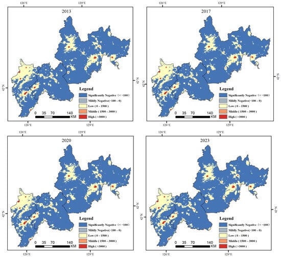
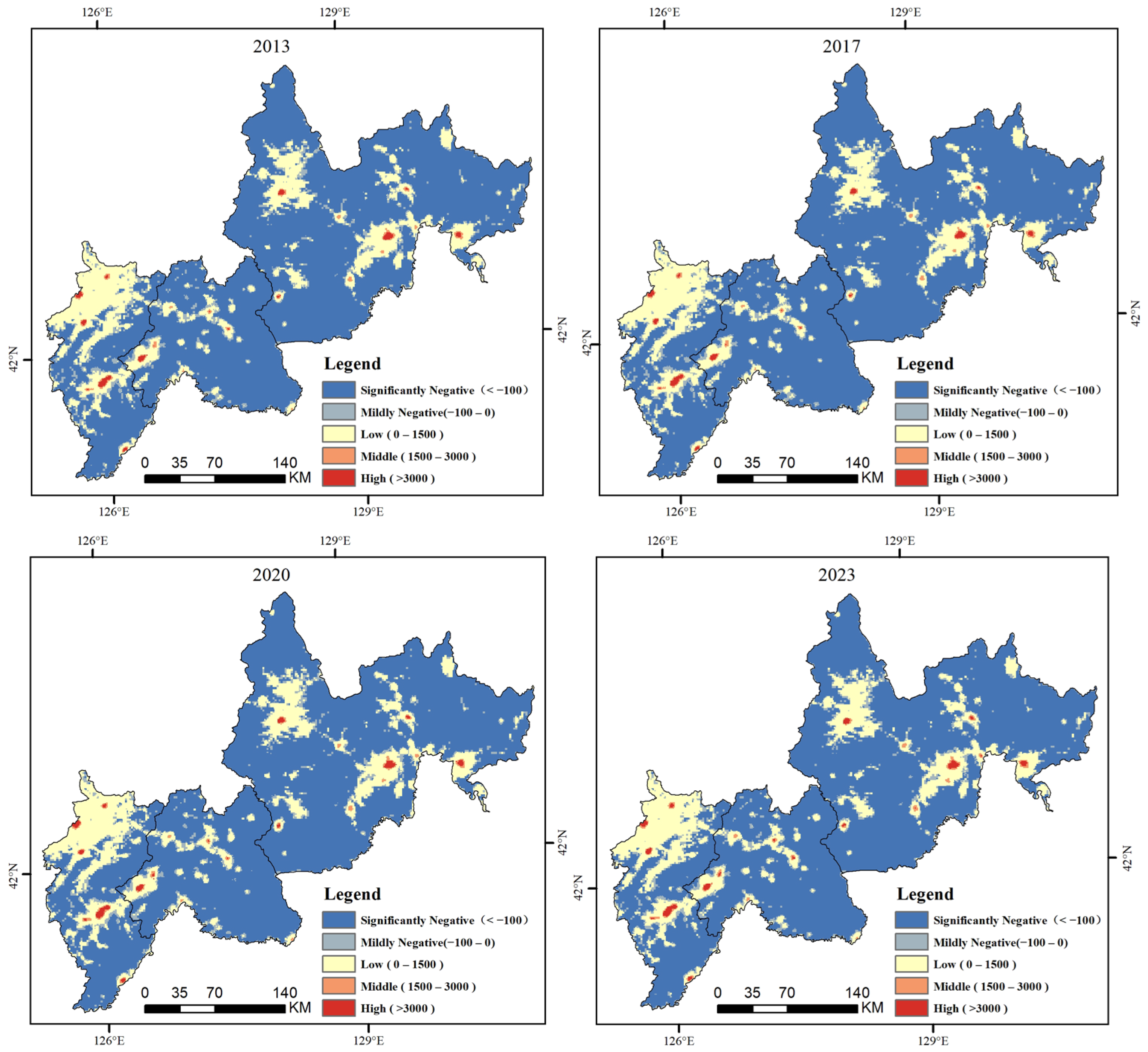
We quantified and classified the LCE of the JLBCs into five classifications (Figure 3). Benefiting from abundant forest resources, the LCE in the three prefecture-level regions of Tonghua, Baishan, and Yanbian in Jilin Province remained negative between 2013 and 2023. However, a distinct upward trend was observed, with total emissions increasing from −9.19 Mt in 2013 to −8.12 Mt in 2023. The most rapid increase occurred between 2020 and 2023, rising from −8.68 Mt to −8.12 Mt. This acceleration is closely associated with the rapid economic recovery and the intensified processes of regional economic development, industrialization, and urbanization during this period.

Figure 3. 2013–2023 LCE map for JLBCs.

In terms of proportional composition, the area classified as significantly negative decreased, while zones with medium-to-high emissions expanded. Although significantly negative areas continued to dominate, their proportion gradually declined. By 2023, their extent had reduced to 56,987.38 km², accounting for 74.82% of the total area. This indicates a gradual weakening of the region’s overall carbon sequestration capacity, despite it remaining dominant. The proportion of mildly negative areas remained relatively stable at approximately 7%, suggesting consistent carbon absorption capacity in these zones. The share of low-emission areas continued to rise, while the proportions of medium- and high-emission zones, though small, also exhibited an upward trend. This implies a gradual expansion of areas with increasing carbon emissions, likely linked to factors such as accelerated urbanization and the expansion of construction land. Notably, high-value emission zones are concentrated in central urban districts, certain city centers (e.g., Dunhua City and Hunchun City), and the predominantly cultivated northern region of Tonghua City.

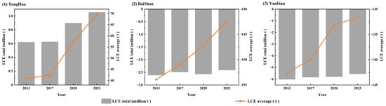
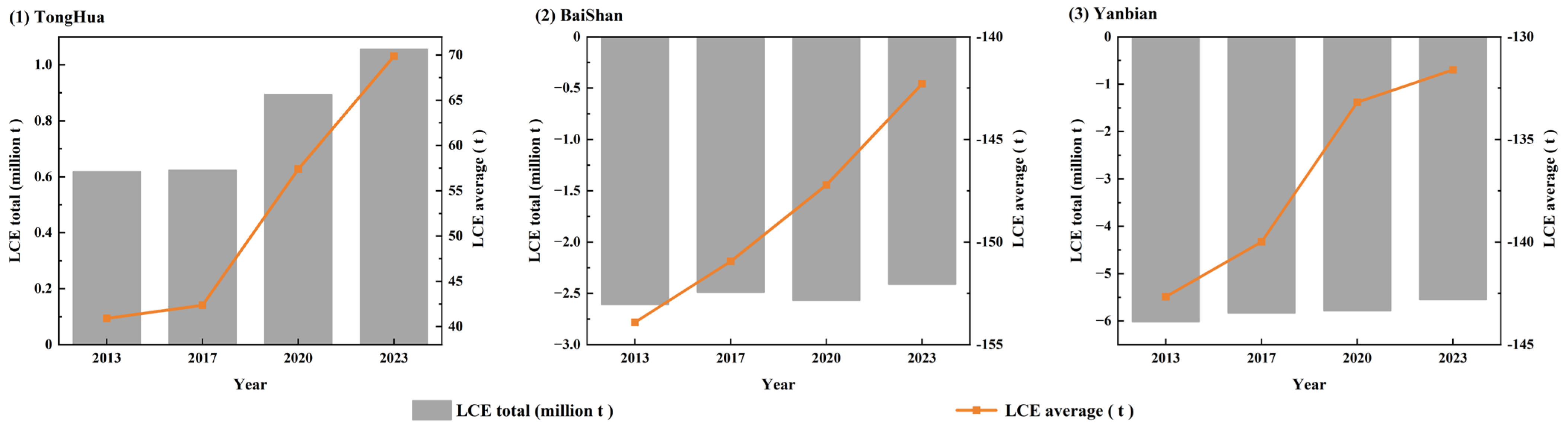
Furthermore, we analyzed the changes in total and average LCE for the JLBCs (Figure 4), revealing distinct carbon emission characteristics among the three prefecture-level regions. In terms of total emissions, Tonghua City exhibited significant growth, whereas Baishan City showed fluctuating increases, and Yanbian Prefecture also demonstrated an increasing trend. Regarding average emissions, all three cities displayed an upward trajectory. Although Baishan City’s total emissions remained negative, the magnitude of this negative value has gradually diminished. Fluctuations during this period may be attributed to adjustments in industrial projects. For Yanbian Prefecture, both total and average emissions continued to increase, but the growth rate slowed between 2020 and 2023. This deceleration may stem from diminishing marginal returns on earlier emission reduction measures or the industrial transition entering a plateau phase, where the scope for adjusting high-carbon industries has narrowed. Overall, Tonghua City experienced positive growth in carbon emissions, while the negative emission effect in Baishan City and Yanbian Prefecture is weakening. The disparities among the three cities are closely related to differences in economic structure, industrial policy, and carbon management efforts.

Figure 4. Total and mean change in LCE for JLBCs.

4.2. ESI Grading Results

The comprehensive ESI was obtained by evaluating and calculating the ten years from 2013 to 2023 in the JLBCs through the ecological safety model. In order to partition the comprehensive evaluation results, the natural breakpoint grading method was used to classify the safety index values into five levels: no warning, light warning, moderate warning, severe warning, and extreme warning, and the ranges and divisions of the specific indexes are shown in Table 2.

Table 2. Classification of the ESI.

Level	Eco-Safety Composite Index Range	Ecological Security Status
Level 1	<0.37	Extreme warning (EW)
Level 2	0.37–0.42	Severe warning (SW)
Level 3	0.42–0.48	Moderate warning (MW)
Level 4	0.48–0.56	Light warning (LW)
Level 5	>0.56	No warning (NW)

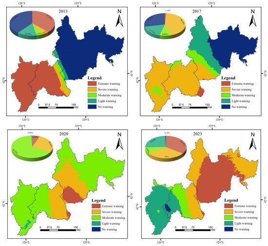
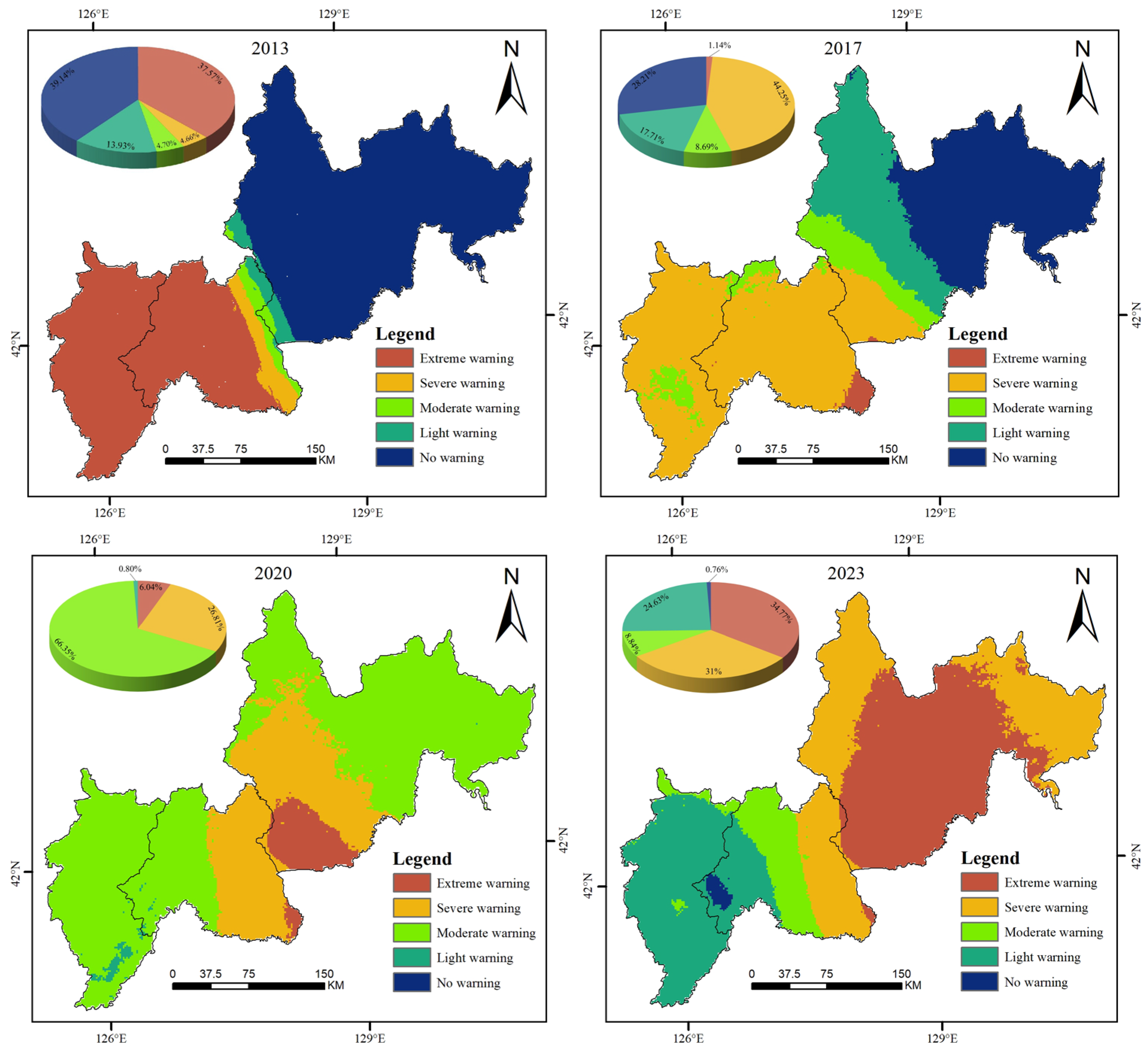
The ecological security of the JLBCs in 2013, 2017, 2020, and 2023 was evaluated using the ecological security evaluation model and classified and partitioned, and the results are shown in Figure 5.

Figure 5. ESI classification map of JLBCs.

Between 2013 and 2023, the ESI of JLBCs underwent significant changes. With the central region serving as a dividing line, ecological security improved in the western areas, while the eastern regions exhibited a deteriorating trend. Specifically, the ecological conditions in Tonghua and Baishan cities continued to improve; conversely, the ESI of Yanbian Prefecture declined continuously, indicating distinct ecosystem degradation.

Overall, the ESI of JLBCs is poor, and the sharp increase in the area of extreme warning zones highlights the problem of overall ecological deterioration. Regarding the statistics of graded areas, the area classified as EW initially declined before rising continuously, dropping from 28,199.29 km² in 2013 to 856.67 km² in 2017, and subsequently increasing to 2610.51 km² in 2023. The significant rise in its proportion during the later stage reflects an intensified threat to ecological security in certain phases. The area of SW fluctuated significantly, characterized by unstable improvement trends and persistent potential ecological risks. The area of MW increased substantially from 3524.00 km² in 2013 to 49,722.29 km² in 2020 but plummeted to 6636.48 km² in 2023. Such drastic fluctuations, potentially influenced by phased environmental pressures, human intervention, or cyclical economic volatility under epidemic prevention measures, indicate poor ecological stability. The area of LW, aside from a drop to 599.03 km² in 2020, showed an overall upward trend, with its proportion rising from 13.94% in 2013 to 24.63% in 2023. The significant fluctuation in 2020 suggests that the ecological status of these areas is highly susceptible to short-term factors or local measures, lacking continuity. The area of NW shrank from 29,374.99 km² in 2013 to 21,199.68 km² in 2017 and disappeared entirely in 2020. By 2023, a small portion recovered to approximately 571.30 km² (0.76%). This overall drastic shrinkage highlights a decline in the region’s ecological security level and the severe compression of high-quality ecological space.

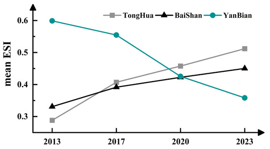
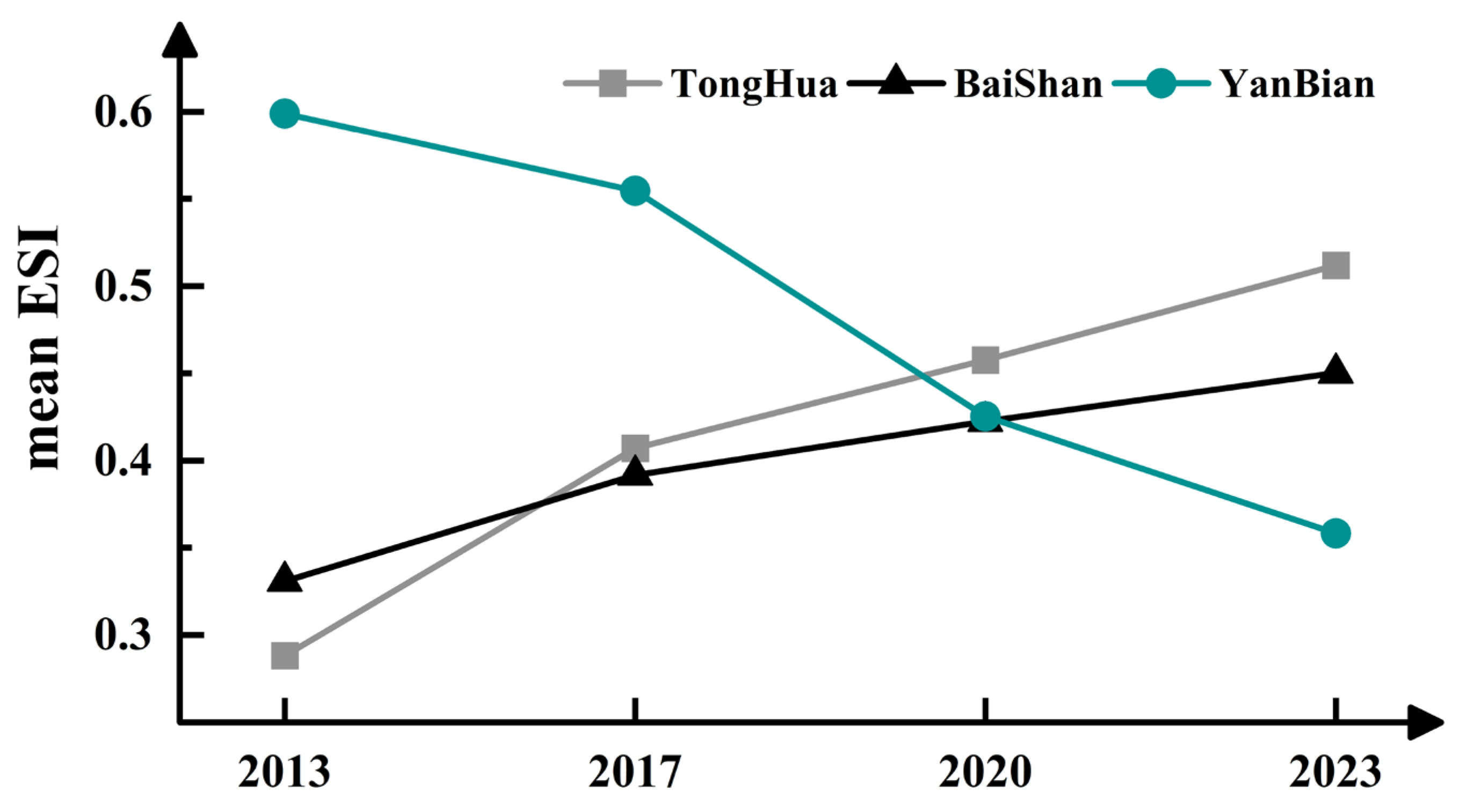
Meanwhile, we calculated the year-by-year mean values of the three cities (states), as shown in Figure 6. From 2013 to 2023, the average ESI of JLBCs shows an upward trend for Tonghua and Baishan, indicating continuous improvement in their ecological security conditions. On the other hand, Yanbian Autonomous Prefecture exhibits a significant downward trend, dropping from 0.598 in 2013 to 0.352 in 2023. This marked decline necessitates targeted measures to enhance ecological security levels and promote sustainable regional ecological development.

Figure 6. Change in mean value of JLBCs’ ESI per city (prefecture).

4.3. Multi-Scale Coupling Degree Analysis of the LCE and ESI

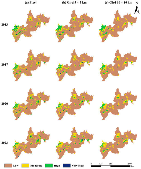
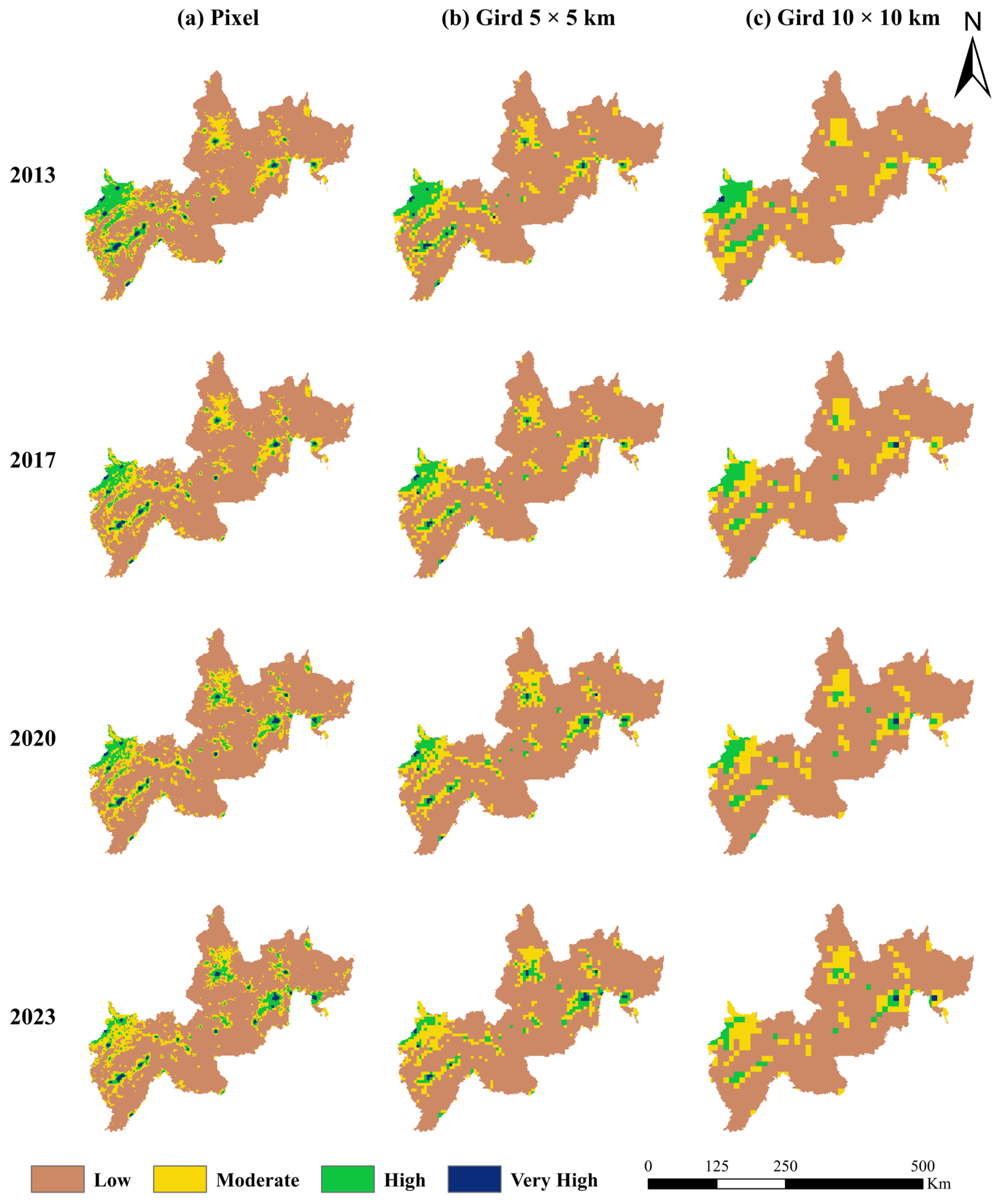
The results of the interaction strength between LCE and the ESI at different scales were obtained using the CD model and are shown in Figure 7.

Figure 7. Multi-scale coupling analysis of LCE and the ESI.

The spatial disparity in the coupling between LCE and the ESI is significant, predominantly characterized by low coupling. Within the same year, a larger scale corresponds to a higher proportion of low coupling values. The most pronounced characteristics of coupling variation are observed in northern Tonghua City, the urban districts of Tonghua and Baishan, Yanbian Prefecture, Dunhua City, and Hunchun City. From a temporal perspective, the coupling degree between LCE and ecological security exhibits distinct variation characteristics across different scales. At the pixel scale, the area of low coupling zones fluctuated minimally between 2013 and 2023, accounting for approximately 77% of the total area. Conversely, the area and proportion of moderate coupling zones continued to increase, rising from 14.93% to 15.91%. High coupling zones displayed a fluctuating downward trend, decreasing from 7.13% to 5.77%, while very high coupling zones showed negligible fluctuation, with their proportion declining slightly from 0.93% to 0.91%. At the 5 × 5 km grid scale, low coupling zones remained dominant (approximately 80%), exhibiting a trend of initial increase followed by a decrease in area. The proportion of moderate coupling zones increased significantly from 12.78% to 14.88%, whereas the proportion of high coupling zones declined from 6.60% to 5.18%, and the area of very high coupling zones fluctuated. At the 10 × 10 km grid scale, the proportion of low coupling zones remained stable at around 80%. The proportion of moderate coupling zones saw a significant rise from 13.14% to 15.25%, while both the area and proportion of high coupling zones decreased. In contrast, the very high coupling zone exhibited an upward trend, reaching a proportion of 0.27% in 2023.

Overall, the multi-scale coupling degree of the region continues to weaken in time, and spatially presents the distribution characteristics of “the larger the scale, the higher the coupling degree”, which reveals the regular differences in the temporal evolution and spatial distribution of the coupling relationship between land use carbon emission and ecological security in the region, and provides data for the management of a multi-scale economic and ecological environment.

4.4. Spatial Relationship Between the Coupling of LCE and ESI

4.4.1. Global Spatial Autocorrelation

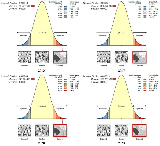
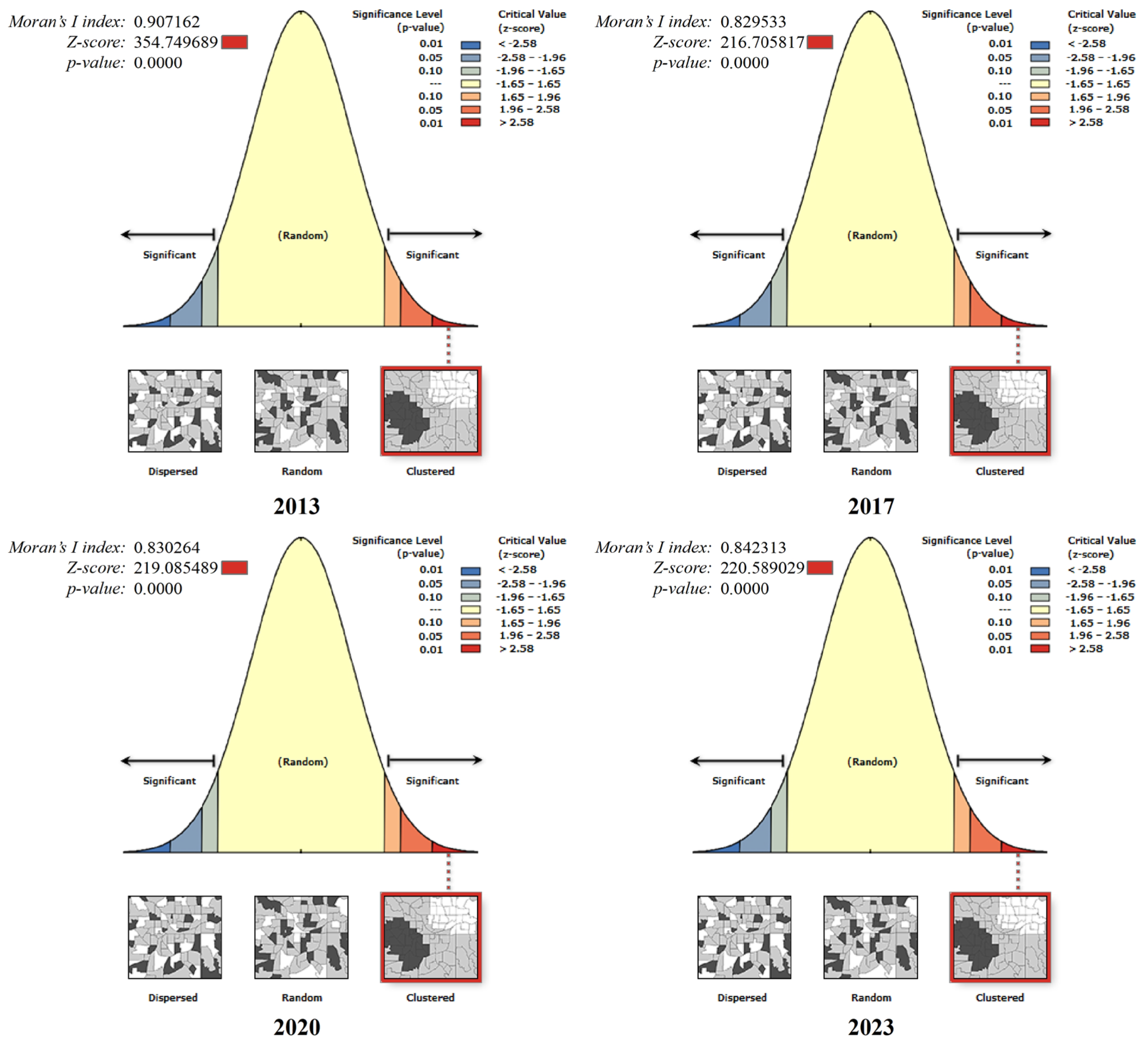
We used ArcGIS 10.8 to calculate the global spatial autocorrelation of the coupling degree, and the results are shown in Figure 8. The Moran’s I index for the years 2013–2023 is 0.90, 0.82, 0.83, and 0.84, respectively, with the p-value of less than 0.01, and the Z scores are 354.74, 216.70, 219.08, and 220.58, respectively, which are much larger than 2.58. This indicates that the coupling degree of LCE and the ESI in the JLBCs is not randomly distributed, but exhibits a significant positive correlation and distinct spatial agglomeration characteristics.

Figure 8. Global spatial autocorrelation analysis results of the coupling between LCE and the ESI.

4.4.2. Local Spatial Autocorrelation

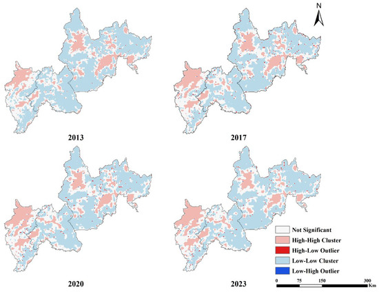
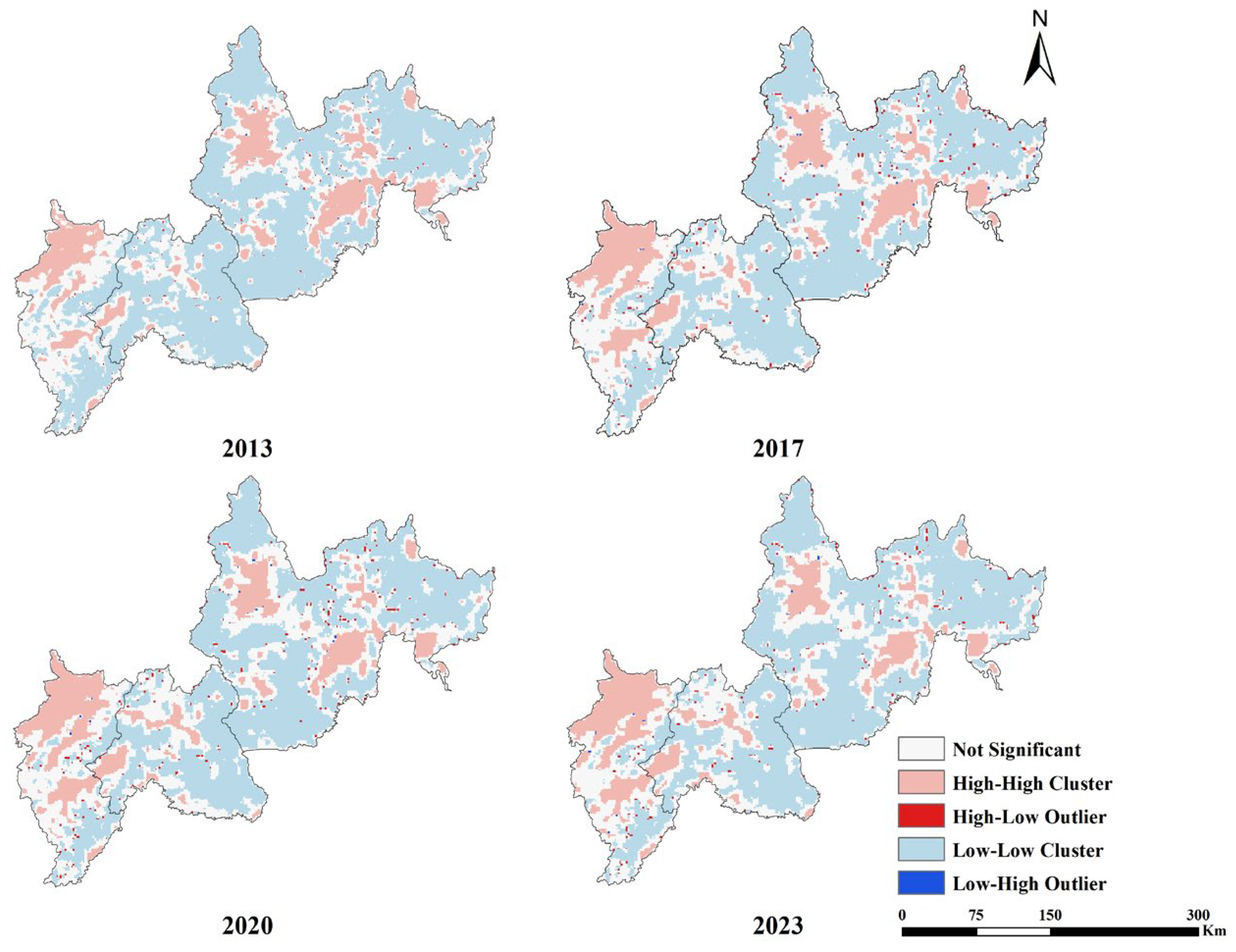
The agglomeration type distribution of the spatial distribution of LCE and the ESI coupling degree contains four types, such as high–high type agglomeration (HH), high–low type agglomeration (HL), low–high type agglomeration (LH), and low–low type agglomeration (LL). The spatial distribution of the local Moran’s index corresponding to the coupling degree of LCE and the ESI is shown in Figure 9. The coupling degree of LCE and the ESI in JLBCs is mainly dominated by the LL clusters, the HH clusters, and the non-significant area.

Figure 9. Local spatial autocorrelation analysis of the coupling between LCE and the ESI.

LL clusters constitute the most extensive category, with area proportions of 56.23%, 50.08%, 49.88%, and 50.82% across the 2013–2023 period, exhibiting a trend of initial decline followed by a slight recovery. These areas are mainly distributed in the vast forest regions of Baishan City and Yanbian Prefecture. HH clusters account for approximately 15% of the total area, primarily concentrated in northern Tonghua City and its central urban districts. In contrast, HL and LH clusters display limited distribution ranges and scattered patterns, often appearing as “associated” distributions along the periphery of LL clusters.

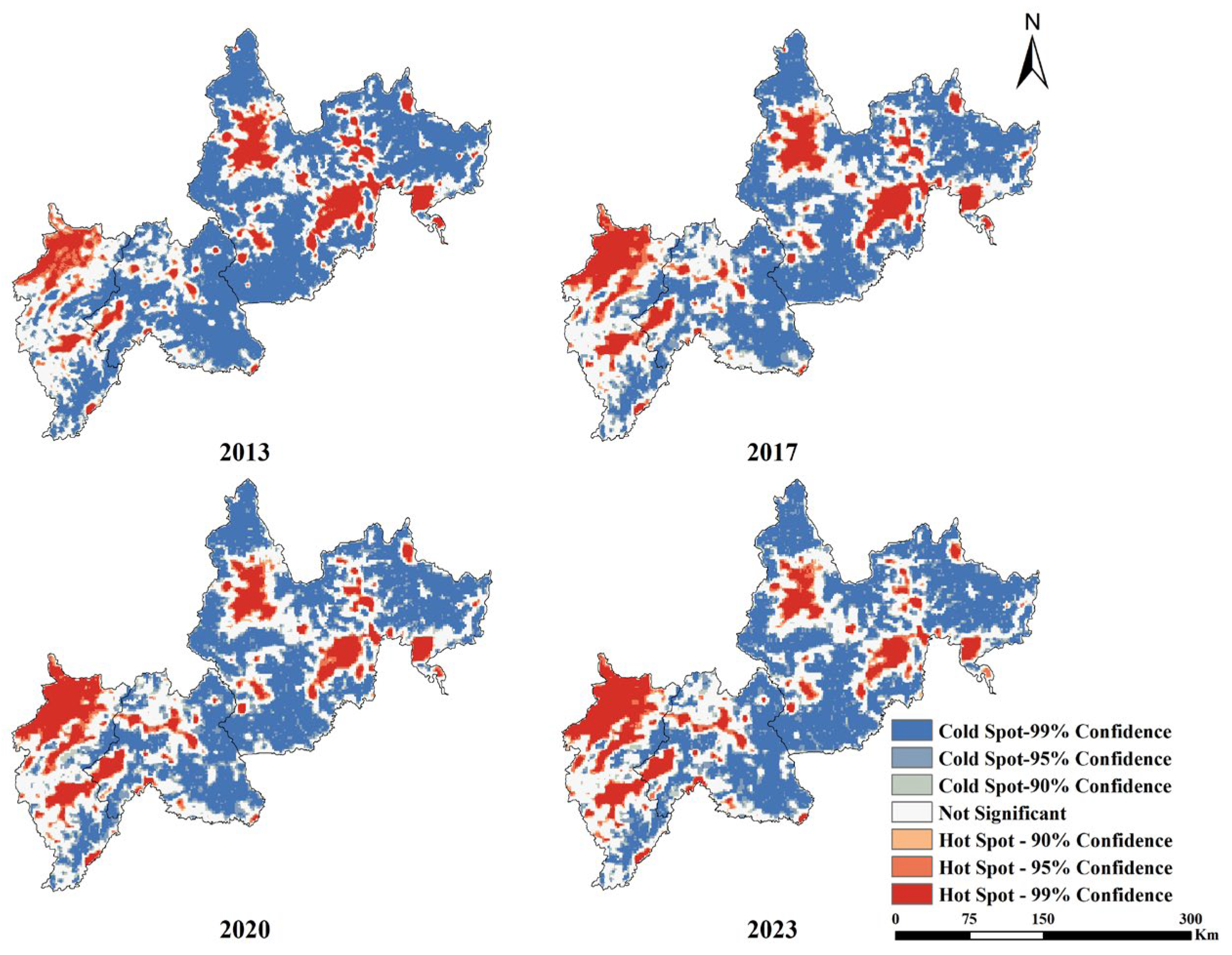
4.4.3. Cold and Hot Spot Analysis

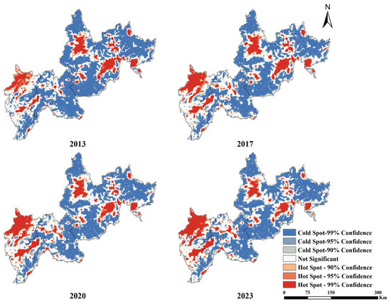
The hot spot analysis yielded high- and low-value clustering areas with different confidence intervals, as shown in Figure 10. The cold and hot spots in the study area are unevenly distributed and are mainly dominated by cold spots, accounting for more than 50% of the total area, and the hot spot areas are in the range of 16–19%. Cold spot areas are mainly distributed in vast forest areas. These forest areas have good vegetation and ecology, but the level of social development in the region is relatively weak and the coupling degree is poor, so cold spots are formed. Hot spot areas are primarily concentrated in northern Tonghua City and other major urban districts. These regions exhibit relatively stable socioecological conditions and relatively developed economies, characterized by high-carbon emissions and strong coupling, thereby forming hot spot clusters. Compared to coupling analysis, hot spot/cold spot analysis provides a more detailed revelation of the spatial distribution patterns of LCE–ESI coupling, enabling precise identification of target areas for regional economic–social–ecological sustainable development.

Figure 10. Cold/hot spot analysis of the coupling between LCE and the ESI.

5. Discussions

5.1. Analysis of the Causes of LCE from LUCCs

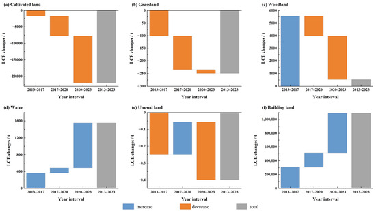
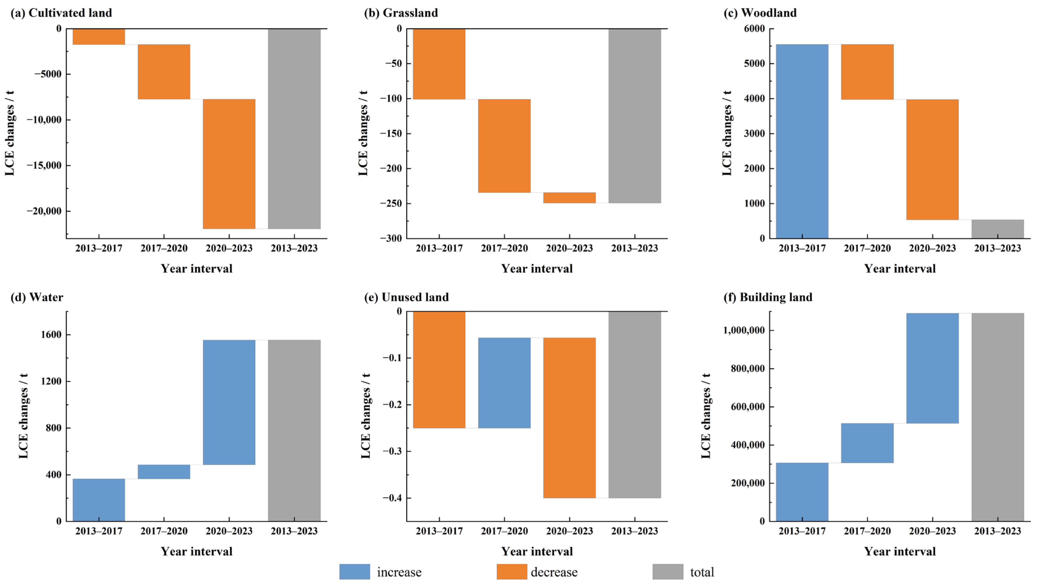
Based on the 2013–2023 LCE map of JLBCs in Figure 2, we explored the changes in LCE caused by land use changes and obtained data on the changes in carbon emissions of different land use types in four periods: 2013–2017, 2017–2020, 2020–2023, and 2013–2023, as shown in Figure 11.

Figure 11. Changes in LCE from different land use types.

Research indicates that construction land serves as the primary source of carbon emissions. The LCE driven by its changes exhibits a significant positive value and a continuous upward trend, with cumulative carbon emissions reaching 1.09 Mt between 2013 and 2023. This phenomenon is closely linked to the surge in energy consumption resulting from the expansion of buildings and infrastructure during urbanization and industrialization. Carbon emissions induced by changes in water bodies have also continued to rise, totaling 1553.33 t from 2013 to 2023, suggesting that these watersheds are being encroached upon and that the reduction in area is exacerbating carbon emissions.

Cultivated land demonstrated negative carbon emissions across all stages, with the absolute value gradually increasing. This indicates a continuous reduction in emissions attributable to cultivated land, likely due to a decrease in cultivated area or the optimization of farming practices. Grasslands generally exhibited a state of negative emissions, characterized by significant emission reductions in the early stages and a narrowing margin of reduction in later stages. Conversely, woodlands showed an increase in carbon emissions in the early period but maintained continuous negative emissions from 2017 to 2023, with total emissions of 537.24 t. The increased emissions during 2013–2017 may be associated with rapid urbanization encroaching on forest land and deforestation for construction timber, which significantly reduced forest area and weakened carbon sinks, whereas the subsequent reduction in emissions is likely related to forest conservation policies in Northeast China. Regarding unused land, the variation in carbon emissions is negligible, exerting a weak impact on the overall carbon balance.

5.2. Area Conversion for Different Ecological Security Levels

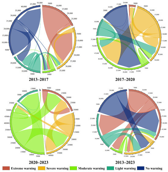
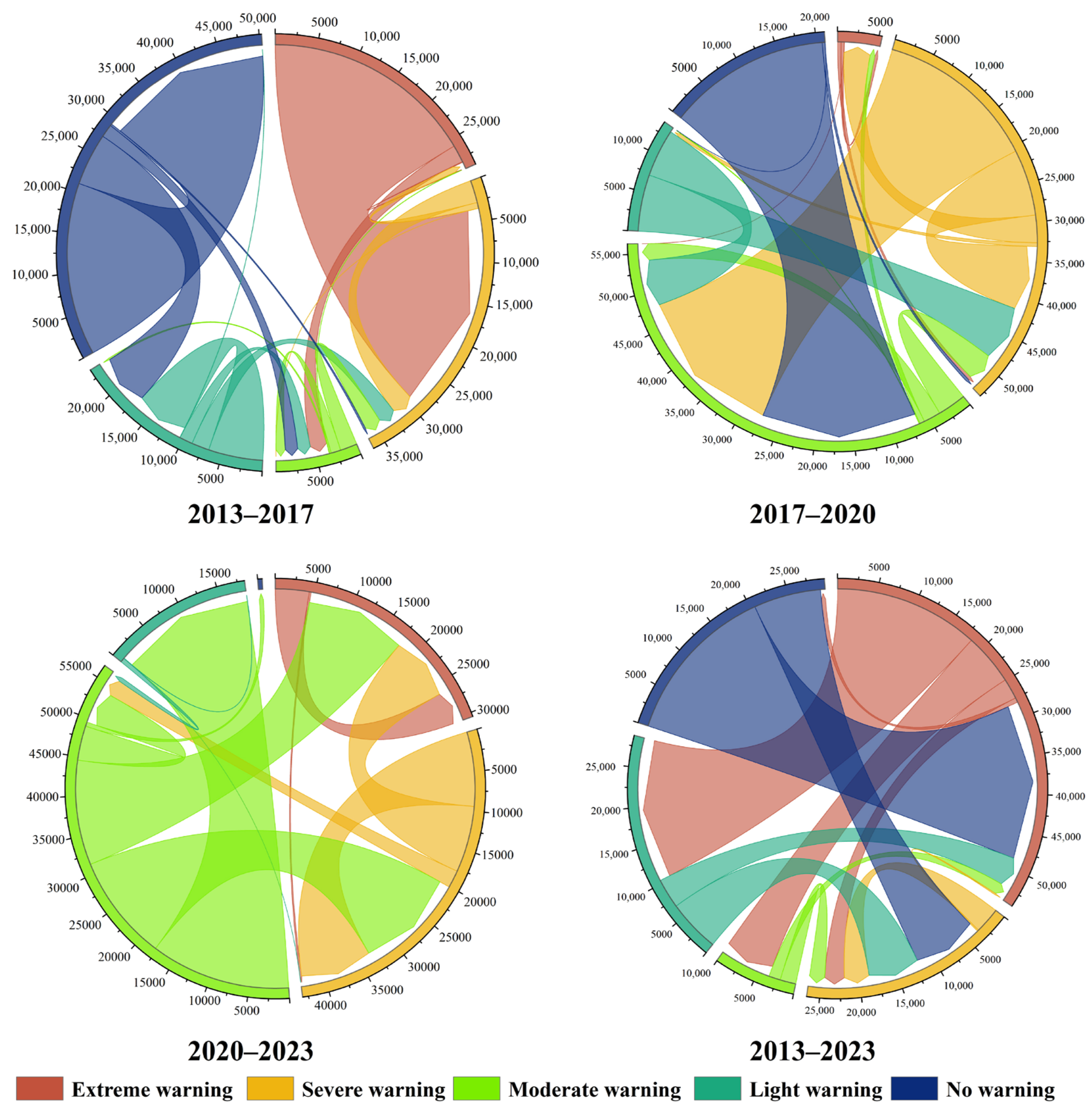
According to the ecological security early warning zoning map shown in Figure 5, the transformation matrices of different categories of ecological security zoning for the four periods of 2013–2017, 2017–2020, 2020–2023, and 2013–2023 were obtained by using the spatial analysis function of ArcGIS, the transfer area table was obtained (as shown in Table 3), and the transformation matrices were visualized to form the transfer chord diagram, as shown in Figure 12.

Table 3. ESI transfer matrix for different stages.

Type of Transfer—Out	Type of Transfer—In
		ESI Transfer Matrix (2013–2017)					ESI Transfer Matrix (2017–2020)
		EW	SW	MW	LW	NW	EW	SW	MW	LW	NW
	EW	83.2	25,847.05	2118.79	0	0	413.22	438.18	5.55	0	0
	SW	723.83	2737.24	2.77	0	0	3488.8	8439.12	20,699.82	499.19	0
	MW	36.05	2063.33	1192.51	196.9	0	626.76	3646.87	2190.9	97.07	0
	LW	0	2146.53	1608.51	6647.57	27.73	0	7207.78	6079.05	0	0
	NW	0	227.41	1575.23	6381.34	21,038.17	0	354.98	20,746.97	2.77	0
		ESI Transfer Matrix (2020–2023)					ESI Transfer Matrix (2013–2023)
		EW	SW	MW	LW	NW	EW	SW	MW	LW	NW
	EW	4295.82	232.96	0	0	0	0	2601.34	6536.64	18,339.76	571.30
	SW	8414.16	9429.18	2221.4	0	0	171.94	3291.89	0	0	0
	MW	13,306.24	13,486.5	4376.25	17,776.78	532.47	1475.39	2007.86	0	0	0
	LW	0	2.77	551.88	38.83	0	3760.58	6664.21	0	0	0
	NW	0	0	0	0	0	20,597.21	8530.63	0	0	0

Figure 12. ESI transfer chord diagrams for different phases.

From a long-term perspective (2013–2023), the SW to MW and LW was particularly significant, with areas of 6536.64 km² and 18,339.76 km², respectively, reflecting a gradual mitigation of risks in severe warning zones. However, the NW areas were completely transformed into EW and SW zones, covering 20,597.21 km² and 8530.63 km², respectively. This indicates that previously safe areas are being encroached upon by high risk levels, posing severe challenges to ecological security. Additionally, bidirectional transfers between LW and SW suggest fluctuations in ecological security levels in certain areas, which have not yet fully stabilized.

From a phased perspective, between 2013 and 2017, transitions were concentrated within higher warning levels. The transfer from EW to SW was particularly pronounced, covering 25,847.05 km², reflecting drastic fluctuations in ecological security status at local levels during this period. While SW zones retained 2737.24 km², minor transfers to MW indicated a trend toward conversion to lighter warning levels. From 2017 to 2020, transfers between ecological security levels were highly active. The most prominent transitions were from SW to MW (20,699.82 km²) and from NW to SW (20,746.97 km²). This demonstrates a distinct divergence in regional ecological security trends during this period: while some areas improved to lower warning levels, others deteriorated. During 2020–2023, significant transfers occurred from MW to both LW and higher warning levels, indicating a continuing polarization trend in ecological security conditions. Although a small portion of areas reverted to NW, marking a slight restoration of the ecological security structure, the overall situation remained complex.

Overall, the ecological security levels in the JLBCs exhibited distinct dominant transfer patterns across different stages, characterized mainly by positive risk mitigation in certain levels and the erosion of no-warning areas. These findings provide data support for regional ecological protection and governance, facilitating targeted measures and continuous monitoring of dynamics at all levels to promote the overall improvement and stabilization of ecological security.

5.3. Imbalanced Distribution and Sustainable Development of the Coupling Effect of LCE and ESI

This study analyzed and mapped the spatial distribution characteristics, spatial correlation intensity, and spatial relationship between LCE and the ESI in JLBCs from 2013 to 2023. Both LCE and the ESI showed uneven distribution.

Economically developed regions typically exhibit higher energy consumption, leading to significantly elevated LCE. This suggests that socioeconomic development is a primary driver of energy consumption and the subsequent rise in LCE, with construction land identified as the major emission source—a conclusion consistent with Chen et al. [38]. Over the past decade, despite being rich in forest resources and acting primarily as carbon sinks, the three border prefectures in Jilin Province experienced a continuous and accelerating rise in total LCE. This indicates that the region has not yet reached its carbon peak. Consequently, future strategies must prioritize the implementation of carbon reduction policies and the preservation of carbon sequestration capacity to maintain regional carbon balance and achieve the goals of “carbon peaking and carbon neutrality”.

Between 2013 and 2023, the ecological security status of JLBCs underwent significant shifts, characterized by a spatial divergence: gradual improvement in the west versus continuous deterioration in the east. The western trend aligns with findings by Zou et al. [39] regarding China–Myanmar border cities, while the eastern trend presents a contrast. Areas of EW and SW have increased, signaling severe encroachment on high-quality ecological space. Conversely, an increase in areas under light warning suggests the efficacy of localized conservation measures. Overall, constrained by socioecological factors, the ecological security of these cities remains precarious. This study emphasizes the holistic impact of these factors to optimize regional ecological security patterns and foster sustainable development.

Significant spatial disparities were observed in the coupling between LCE and the ESI, which was predominantly characterized by low-degree coupling. From 2013 to 2023, low-degree coupling areas remained stable (77–80%), while medium-degree coupling areas expanded to an average of 15.34%, and high-degree coupling areas exhibited a fluctuating decline. These spatial dynamics were most pronounced in northern Tonghua, the urban centers of Tonghua and Baishan, Yanbian Prefecture, Dunhua, and Hunchun. The imbalance in LCE–ESI coupling is intrinsically linked to the spatial distribution of socioeconomic and natural conditions. By examining the classic economy–environment relationship within the unique context of the northeast border, this study reveals a spatial mismatch between economic and ecological advantages. It proposes regional interaction as a mechanism to mitigate these disparities, offering actionable pathways for sustainable border development.

Furthermore, balancing border risks with the advantages of cross-border exchange is critical for the sustainable development of border cities, where ports serve as strategic gateways. The development of northeast border cities necessitates a comprehensive assessment of socioecological drivers, pressures, states, impacts, responses, and management. Key measures include promoting economic growth, deepening bilateral cooperation on non-traditional security issues to mitigate disaster risks, and advocating for shared sustainable development principles in economic and ecological governance. These efforts aim to cultivate a positive, integrated economic, social, and ecological environment in Northeast Asia.

6. Conclusions

This study systematically analyzed the spatiotemporal evolution characteristics of LCE and the ESI in the JLBCs from 2013 to 2023. By employing a coupling degree model, the research revealed the synergistic relationship between LCE and the ESI and conducted a comprehensive spatial analysis of their coupling degree. Furthermore, the study investigated the causes of LCE driven by land use changes, analyzed area variations across different ecological security levels, and evaluated the spatial heterogeneity and sustainability of the coupling effects. The main conclusions are as follows:

(1)

The spatiotemporal differentiation patterns and driving mechanisms of LCE were revealed. The study found that high-value LCE areas are persistently concentrated in administrative central urban districts, exhibiting a core-periphery structural characteristic. Although the overall LCE maintained a negative carbon sink status, it increased from –9.19 Mt to –8.12 Mt over the decade, indicating a weakening of regional carbon sink capacity. This change is primarily attributed to drastic adjustments in land use structure. The encroachment on forest land and water bodies significantly exacerbated carbon emissions, while the reduction of cultivated land and expansion of grassland somewhat inhibited the growth rate of emissions. These findings clarify that human activity intensity and land use patterns are key factors influencing carbon emissions in border cities.

(2)

The spatial evolution pattern and trend of the ESI were characterized. Between 2013 and 2023, the ecological security status of JLBCs showed significant spatial differentiation: ecological quality in western regions such as Tonghua and Baishan continued to improve, whereas the eastern Yanbian Prefecture faced challenges of ecological degradation. Overall, influenced by rapid urbanization and resource development activities, the regional ESI structure exhibited a downward trend, highlighting a spatial pattern of “stable in the west, deteriorating in the east”. This discovery provides a precise basis for formulating differentiated ecological governance strategies.

(3)

The spatial agglomeration characteristics of the LCE–ESI coupling system were identified. The study found that the coupling degree between LCE and the ESI was generally low, with low coupling types accounting for 77–80% of the total area. Moreover, coupling characteristics were found to be more pronounced at larger spatial scales. Spatial autocorrelation analysis indicated that the coupling degree presented significant positive correlation and spatial clustering, forming agglomeration patterns dominated by LL and HH types. Additionally, hot spots and cold spots within the study area were unevenly distributed, with cold spot zones dominating and accounting for over 50% of the area. This reflects the overlapping dilemma of ecologically fragile areas and low development levels, constituting a major shortcoming for regional sustainable development.

This study not only enriches the theoretical system regarding the synergy between ecological security and carbon emissions in border regions but also holds significant practical value. It is recommended that future policies focus on “zoned strategies and synergistic efficiency”, promoting green low-carbon development models in the western ecological improvement zones while implementing ecological restoration and land use control in the eastern ecological degradation zones. Simultaneously, a cross-border ecological security collaboration mechanism should be established to strengthen cooperation with neighboring countries in ecological protection and carbon sink management, thereby facilitating the synergistic realization of national “dual carbon” goals and border stability strategies.

References

- Xu, S.; Wang, R.; Gasser, T.; Ciais, P.; Peñuelas, J.; Balkanski, Y.; Boucher, O.; Janssens, I.A.; Sardans, J.; Clark, J.H.; et al. Delayed use of bioenergy crops might threaten climate and food security. Nature 2022, 609, 299–306. [Google Scholar] [CrossRef] [Scilit]
- Zhang, T.; van der Wiel, K.; Wei, T.; Screen, J.; Yue, X.; Zheng, B.; Selten, F.; Bintanja, R.; Anderson, W.; Blackport, R.; et al. Increased wheat price spikes and larger economic inequality with 2° global warming. One Earth 2022, 5, 907–916. [Google Scholar] [CrossRef] [Scilit]
- Ombadi, M.; Risser, M.D.; Rhoades, A.M.; Varadharajan, C. A warming-induced reduction in snow fraction amplifies rainfall extremes. Nature 2023, 619, 305–310. [Google Scholar] [CrossRef] [Scilit] [PubMed]
- Rong, T.; Zhang, P.; Zhu, H.; Jiang, L.; Li, Y.; Liu, Z. Spatial correlation evolution and prediction scenario of land use carbon emissions in China. Ecol. Inform. 2022, 71, 101802. [Google Scholar] [CrossRef] [Scilit]
- Zhang, C.-Y.; Zhao, L.; Zhang, H.; Chen, M.-N.; Fang, R.-Y.; Yao, Y.; Zhang, Q.-P.; Wang, Q. Spatial-temporal characteristics of carbon emissions from land use change in Yellow River Delta region, China. Ecol. Indic. 2022, 136, 108623. [Google Scholar] [CrossRef] [Scilit]
- Yang, Y.J.; Li, H.Y. Spatiotemporal dynamic decoupling states of eco-environmental quality and land-use carbon emissions: A case study of Qingdao City, China. Ecol. Inform. 2023, 75, 101992. [Google Scholar] [CrossRef] [Scilit]
- Wang, Q.; Yang, C.-H.; Wang, M.-L.; Zhao, L.; Zhao, Y.-C.; Zhang, Q.-P.; Zhang, C.-Y. Decoupling analysis to assess the impact of land use patterns on carbon emissions: A case study in the Yellow River Delta efficient eco-economic zone, China. J. Clean. Prod. 2023, 412, 137415. [Google Scholar] [CrossRef] [Scilit]
- Zhang, J.; Li, H.; Ren, G.; Zhang, Z.; Nie, S. Advancing sustainable mining Practices: A dynamic ecological security and risk warning framework for ion-absorbed rare earth mine. J. Clean. Prod. 2025, 511, 145630. [Google Scholar] [CrossRef] [Scilit]
- Liu, J.; Peng, K.; Zuo, C.; Li, Q. Spatiotemporal variation of land-use carbon emissions and its implications for low carbon and ecological civilization strategies: Evidence from Xiamen-Zhangzhou-Quanzhou metropolitan circle, China. Sustain. Cities Soc. 2022, 86, 104083. [Google Scholar] [CrossRef] [Scilit]
- Cai, A.; Guo, R.; Zhang, Y.; Wang, L.; Lin, R.; Wu, H.; Huang, R.; Zhang, J.; Wu, J. Assessing urban carbon health in China’s three largest urban agglomerations: Carbon emissions, energy-carbon emission efficiency and carbon sinks. Appl. Energy 2025, 383, 125326. [Google Scholar] [CrossRef] [Scilit]
- Yang, Y.; Li, H. Monitoring spatiotemporal characteristics of land-use carbon emissions and their driving mechanisms in the Yellow River Delta: A grid-scale analysis. Environ. Res. 2022, 214, 114151. [Google Scholar] [CrossRef] [Scilit]
- Gurney, K.R.; Liang, J.; O’KEeffe, D.; Patarasuk, R.; Hutchins, M.; Huang, J.; Rao, P.; Song, Y. Comparison of Global Downscaled Versus Bottom-Up Fossil Fuel CO2 Emissions at the Urban Scale in Four US Urban Areas. J. Geophys. Res.-Atmos. 2019, 124, 2823–2840. [Google Scholar] [CrossRef] [Scilit]
- Basu, S.; Lehman, S.J.; Miller, J.B.; Andrews, A.E.; Sweeney, C.; Gurney, K.R.; Xu, X.; Southon, J.; Tans, P.P. Estimating US fossil fuel CO2 emissions from measurements of 14C in atmospheric CO2. Proc. Natl. Acad. Sci. USA 2020, 117, 13300–13307. [Google Scholar] [CrossRef] [Scilit] [PubMed]
- Ma, J.; Li, J.; Wu, W.; Liu, J. Global forest fragmentation change from 2000 to 2020. Nat. Commun. 2023, 14, 3752. [Google Scholar] [CrossRef] [Scilit] [PubMed]
- Riva, F.; Fahrig, L. Landscape-scale habitat fragmentation is positively related to biodiversity, despite patch-scale ecosystem decay. Ecol. Lett. 2023, 26, 268–277. [Google Scholar] [CrossRef] [Scilit]
- Wang, J.F.; Xiao, H.; Hu, M.X. Spatial spillover effects of forest ecological security on ecological well-being performance in China. J. Clean. Prod. 2023, 418, 13. [Google Scholar] [CrossRef] [Scilit]
- Liu, F.; Zhang, Q.; Wang, J.; Liu, Y.; Wang, W.; Li, S. Ecological security assessment of Yunnan Province, China in the context of Production-Living-Ecological space division. Ecol. Evol. 2024, 14, e70131. [Google Scholar] [CrossRef] [Scilit]
- Zhang, M.; Bao, Y.; Xu, J.; Han, A.; Liu, X.; Zhang, J.; Tong, Z. Ecological security evaluation and ecological regulation approach of East-Liao River basin based on ecological function area. Ecol. Indic. 2021, 132, 108255. [Google Scholar] [CrossRef] [Scilit]
- Du, W.; Liao, X.; Tong, Z.; Rina, S.; Rong, G.; Zhang, J.; Liu, X.; Guo, E. Early warning and scenario simulation of ecological security based on DPSIRM model and Bayesian network: A case study of east Liaohe river in Jilin Province, China. J. Clean. Prod. 2023, 398, 136649. [Google Scholar] [CrossRef] [Scilit]
- Dong, Z.; Zhang, J.; Tong, Z.; Han, A.; Zhi, F. Ecological security assessment of Xilingol grassland in China using DPSIRM model. Ecol. Indic. 2022, 143, 109336. [Google Scholar] [CrossRef] [Scilit]
- An, M.; Xie, P.; He, W.; Wang, B.; Huang, J.; Khanal, R. Local and tele-coupling development between carbon emission and ecologic environment quality. J. Clean. Prod. 2023, 394, 136409. [Google Scholar] [CrossRef] [Scilit]
- Medeiros, A.; Fernandes, C.; Gonçalves, J.F.; Farinha-Marques, P. A diagnostic framework for assessing land-use change impacts on landscape pattern and character-A case-study from the Douro region, Portugal. Landsc. Urban Plan. 2022, 228, 104580. [Google Scholar] [CrossRef] [Scilit]
- Baldi, V.; Bellino, A.; Baldantoni, D. Small-scale land use effects on plant communities in Mediterranean urban ecosystems. Ecol. Indic. 2025, 170, 113051. [Google Scholar] [CrossRef] [Scilit]
- Freeman, C. The desert, the border, and the city: Staging a spectacle on the Chile-Peru border. Political Geogr. 2021, 87, 102380. [Google Scholar] [CrossRef] [Scilit]
- Ma, M.; Yu, Z.; Ma, L.; Guo, W. Institutional openness and city cross-border e-commerce: Evidence from China’s pilot free trade zones. Econ. Anal. Policy 2025, 85, 558–570. [Google Scholar] [CrossRef] [Scilit]
- Zhang, H.; Wang, Y.; Liu, H. Smart cities lighting the way: Optimizing energy structure and efficiency in the border areas. J. Clean. Prod. 2025, 486, 144481. [Google Scholar] [CrossRef] [Scilit]
- Oda, T.; Maksyutov, S. A very high-resolution (1 km×1 km) global fossil fuel CO2 emission inventory derived using a point source database and satellite observations of nighttime lights. Atmos. Chem. Phys. 2011, 11, 543–556. [Google Scholar] [CrossRef] [Scilit]
- Jin, C.; Xue, Y.; Yuan, T.; Zhao, L.; Jiang, X.; Sun, Y.; Wu, S.; Wang, X. Retrieval anthropogenic CO2 emissions from OCO-2 and comparison with gridded emission inventories. J. Clean. Prod. 2024, 448, 13. [Google Scholar] [CrossRef] [Scilit]
- Balamurugan, V.; Chen, J. Fossil Fuel CO2 Emission Signatures Over India Captured by OCO-2 Satellite Measurements. Earths Future 2024, 12, 22. [Google Scholar] [CrossRef] [Scilit] [PubMed]
- Oda, T.; Maksyutov, S.; Andres, R.J. The Open-source Data Inventory for Anthropogenic CO2, version 2016 (ODIAC2016): A global monthly fossil fuel CO2 gridded emissions data product for tracer transport simulations and surface flux inversions. Earth Syst. Sci. Data 2018, 10, 87–107. [Google Scholar] [CrossRef] [Scilit]
- Wei, X.; Zhang, L.; He, Y.; Gao, B.; Yao, S.; Ding, Y.; Guo, Y.; Ran, L. Spatiotemporal Characteristics and Prediction of Ecological Safety in the Yellow River Basin of China. IEEE J. Sel. Top. Appl. Earth Obs. Remote Sens. 2024, 17, 16119–16138. [Google Scholar] [CrossRef] [Scilit]
- Wang, N.; Zhang, Y.X. Research on evaluation of Wuhan air pollution emission level based on entropy weight method. Sci. Rep. 2024, 14, 9. [Google Scholar] [CrossRef] [Scilit] [PubMed]
- Han, D.; Yu, D.; Qiu, J. Assessing coupling interactions in a safe and just operating space for regional sustainability. Nat. Commun. 2023, 14, 1369. [Google Scholar] [CrossRef] [Scilit]
- Huang, Z.; Chen, Y.; Zheng, Z.; Wu, Z. Spatiotemporal coupling analysis between human footprint and ecosystem service value in the highly urbanized Pearl River Delta urban Agglomeration, China. Ecol. Indic. 2023, 148, 110033. [Google Scholar] [CrossRef] [Scilit]
- Moran, P.A.P. Notes on Continuous Stochastic Phenomena. Biometrika 1950, 37, 17–23. [Google Scholar] [CrossRef] [Scilit]
- Yang, X.; Li, H.; Zhang, J.; Niu, S.; Miao, M. Urban economic resilience within the Yangtze River Delta urban agglomeration: Exploring spatially correlated network and spatial heterogeneity. Sustain. Cities Soc. 2024, 103, 16. [Google Scholar] [CrossRef] [Scilit]
- Getis, A.; Ord, J.K. The Analysis of Spatial Association by Use of Distance Statistics. Geogr. Anal. 1992, 24, 189–206. [Google Scholar] [CrossRef] [Scilit]
- Chen, S.; Cai, X.; Lian, X.; Zhang, H. Influencing factors and spatiotemporal heterogeneity of land-use carbon emissions in China’s urban agglomerations. Sci. Rep. 2026, 16, 2083. [Google Scholar] [CrossRef] [Scilit] [PubMed]
- Zou, Y.; Wang, S.; Luo, X.; Jin, H.; Xiao, X.; Li, Y. A new multivariate index for ecological security assessment in the China-Myanmar border region. J. Environ. Manag. 2024, 364, 14. [Google Scholar] [CrossRef] [Scilit] [PubMed]
Disclaimer/Publisher’s Note: The statements, opinions and data contained in all publications are solely those of the individual author(s) and contributor(s) and not of MDPI and/or the editor(s). MDPI and/or the editor(s) disclaim responsibility for any injury to people or property resulting from any ideas, methods, instructions or products referred to in the content. |
© 2026 by the authors. Licensee MDPI, Basel, Switzerland. This article is an open access article distributed under the terms and conditions of the Creative Commons Attribution (CC BY) license.