


Abstract
With the increasing number of wildfire events, people living close to the wildland–urban interface (WUI) are more likely to be exposed to these events. To mitigate the hazards related to wildfires, it is of great importance to identify areas where human settlements are at a greater risk. Remote sensing-based techniques for mapping and quantifying the inhabitants possibly affected by these events are crucial to reduce the loss of life as well as reduce the negative impact that wildfires pose to the people living in WUIs, the surrounding areas, and the environment. Fine-scale mapping is a suitable auxiliary tool to indicate areas at greater risk. Hence, the dasymetric method was applied to generate a high-resolution map of the study area’s population, using products generated from Sentinel-2 imagery, a census, and Light Detection and Ranging (LiDAR) data. The findings of the proposed methodology show that around 59% of the population in the study area currently lives inside the WUI, while in 2025, most of the people affected by wildfires—77%—lived outside the WUI. This is expected, since wildfires vary in space and time, and they are seen as spatial–temporal processes. In addition, the results demonstrated that women are slightly more exposed to wildfires than other population groups. These results showed that the proposed methodology could not only help identify high-risk areas but also the number of people living in these areas due to the high-resolution dasymetric methodology. The proposed methodology described in this work shows that fine-scale mapping could enrich forest management in order to protect the populations susceptible to the negative impacts of wildfires, consequently protecting the environment.
1. Introduction
Wildfire is a natural process in many ecosystems and can threaten the environment and wildlife [1]. The increasing frequency and severity of extreme wildfire events also elevate risks to human life, particularly for people living near vegetation and other fuels such as shrublands [2]. These areas are known as the wildland–urban interface (WUI). Although definitions vary across countries, for example, a study from the United States of America (USA) defines the WUI as where buildings meet wildland vegetation and the risk of human and environmental conflicts can be concentrated [3], and in a study from Argentina, they used the same definition applied in the USA [4]. A study by Modugno et al. [5], for some European countries, defines the WUI as a landscape where human settlements and forest fuels are in contact. But for each definition, they converge on a similar concept: the WUI is the zone where human settlements meet or intermingle with wildland vegetation [6].
Houses built close to these areas face two main problems related to wildfire: (1) Human ignitions can increase the number of events [4]; (2) these events put lives and homes at risk within these areas [7]. Moreover, these fires are difficult to suppress and allowing them to burn is not feasible. Most work to delineate the WUI uses census data and land-use and land-cover (LULC) maps, such as census blocks and population information, including counts of individuals living in those areas, to identify people exposed to wildfire risks.
Several methods have been developed to delineate the WUI worldwide [2,3,8,9,10], and the same applies to Portugal. Pereira et al. [6] developed a methodology for WUI mapping and defined two interfaces: the direct interface, where urban areas are in immediate physical contact with flammable vegetation, and the indirect interface, where urban areas are less than a pre-specified distance from flammable vegetation. According to the same authors, this methodology is important, because Portugal has seen an increase in wildfires in recent years that affect buildings and inhabitants [11].
Therefore, identifying the WUI is essential for risk assessment, fire prevention, suppression, and land-use planning [6,8]. The proposed methodology for delineating the WUI relies on the national land-cover map (COS) created by the Portuguese Land Planning and Mapping Agency, with a minimum mapping unit of 1 ha. Population density is divided into densely populated areas (cities), intermediate density areas (towns and suburbs), and thinly populated rural areas, where more than 50% of the population lives in rural locations [6]. The latter is the main focus of this research.
It is worth noting that one of the main goals of the study in [6] was to delineate the WUI across mainland Portugal using available spatial LULC data. However, much finer-scale LULC maps can be produced from satellite imagery, such as Sentinel-2, which is freely available from the Copernicus hub [12]. Combining this data with a classification method, such as a machine-learning (ML) approach, supports the creation of fine-scale maps of wildland forests and other land-cover types [13,14]. Beyond satellite imagery, advances in other remote sensing technologies like Light Detection and Ranging (LiDAR) can further enhance the delineation of LULC, the WUI, and residential structures at high spatial resolution [15,16,17].
Furthermore, population density information can also be improved. Rather than relying on block-level census data, since choropleth maps are the most common way to display population data and assume uniform density within each block [3,18], their raster data offer regularly sized units and have a higher resolution when compared to vector data—the most common format used to delineate census blocks. The data can be redistributed to better represent population density and refine spatial detail, using approaches such as the dasymetric method, which transforms the population information from administrative units that can change over time into a population grid that will have the same size cell over time [19,20,21]. In this method, auxiliary datasets such as LULC maps and building polygons can be used to reallocate census counts more realistically [22,23], thereby better representing the actual spatial distribution of the population.
Over time, different methods were developed to desegregate census data into a higher resolution grid. They are divided into three categories: binary dasymetric, which divides the zones into populated and unpopulated areas; multi-class dasymetric, developed by Mennis [24], which incorporates areal weighting and empirical sampling techniques to assess the relationship between categorical and ancillary data and population distribution, assigning different weights to each class category to determine the population density; and finally, intelligent dasymetric mapping. They are complex models, such as ML, that create population spatial distribution data [21,25].
One limitation of the dasymetric mapping method is that populations sparsely inhabiting the area of interest could be overestimated in densely urban areas or underestimated for other land-use classes due to the dataset and spatial resolution, which would not preserve the pycnophylactic property [24]. This means that the sum of the population data for the original set of areal units (e.g., census blocks) is not preserved during the transformation to the new set of areal units.
When delineating the WUI, it is also important to consider Forest Management Units (FMUs), which divide large forest areas into manageable parcels where silvicultural treatments and protection measures can be tailored to local conditions [26,27]. Integrating WUI delineation with FMUs supports the development of sustainable forest management plans, helps mitigate wildfire risk, and protects people and infrastructure by enabling the monitoring of changes at the interface and fostering greater community engagement [10,28,29,30,31].
In this study, we developed a fine-scale mapping approach for northern Portugal using dasymetric methodology, together with LiDAR and satellite imagery, to spatially disaggregate census data to identify populations at risk. We integrate auxiliary information, including satellite imagery [12], the WUI, building data—from LiDAR information, FMUs, census block data, wildfire risk forecasting information, and LULC maps [32]—with the dasymetric areal interpolation method to identify the expected population exposed to wildfire risks within the study area.
We considered the total population and disaggregated it by sex and age to assess the vulnerability of these groups and identify which group may be at higher risk within the study area. Moreover, the methodology could be used as an auxiliary tool in the forest management decision-making process, as the population at risk can be identified, and measures can be taken to reduce their exposure. Although the aim of this work is not to develop strategies to prevent wildfires, the decisions taken to protect the inhabitants of the study area can be further incorporated as a wildfire risk mitigation plan and its actions.
2. Materials and Methods
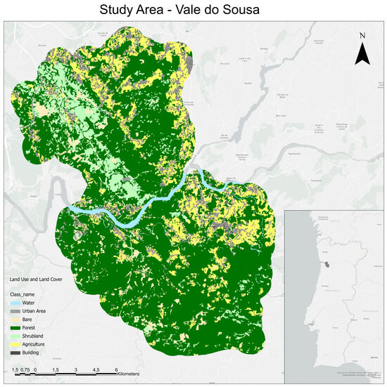
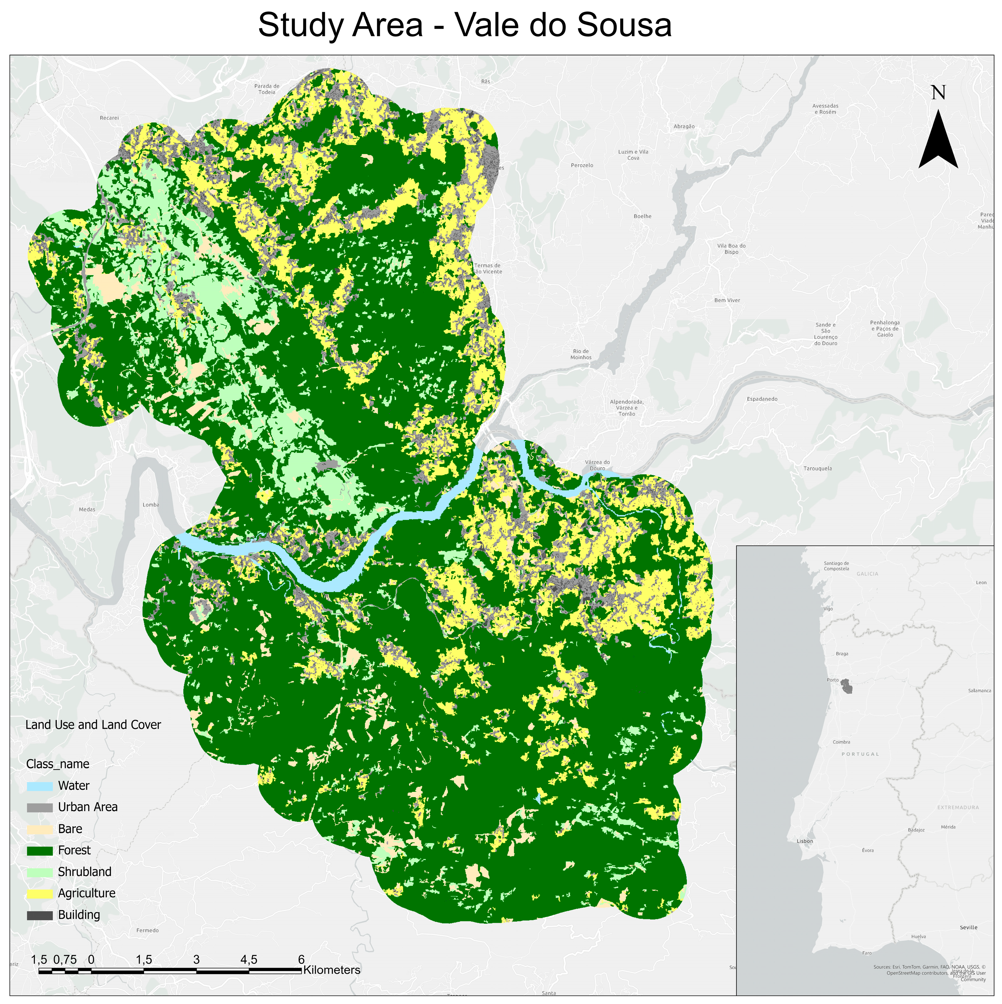
Vale do Sousa Forest (Figure 1) is located in the northern region of Portugal. As in other parts of the country, it has experienced an increase in wildfire events. Residents of this region are also affected by these events [33]. In 2025, more than 3015 hectares burned in the study area; this information was developed using Sentinel-2 imagery [12]. The area of interest (AOI) includes two Forest Intervention Zones (ZIFs). These zones are defined as delimited and contiguous areas, consisting mostly of forests, subject to a forest management plan in accordance with the PMDF and administered by a management entity [34]. In this case, administration is carried out by the Vale do Sousa Forest Association (AFVS) [33]. The landscape is fragmented into more than 340 landholdings grouped by the AFVS. The dominant forest species are eucalypt (Eucalyptus globulus Labill) and maritime pine (Pinus pinaster Aiton), occurring in both pure and mixed stands [34].
Figure 1.
Study area localization with the land-cover classes.
2.1. Remote Sensing Datasets and Demography Information
All remote sensing datasets, including LULC maps, FMUs, wildfire risk forecasts, and building footprints derived from LiDAR (Figure 1), were obtained from prior work evaluating wildfire risk in the study area [32,33]. FMUs were derived from the 2022 LULC and developed using a Support Vector Machine (SVM). Classes, road boundaries, and watersheds were used to delineate each FMU. Building footprints of Vale do Sousa were generated from LiDAR information of the study area surveyed in 2022 during the leaf-on season. Wildfire risk forecasting maps were generated by applying Convolutional Gated Recurrent Unit (ConvGRU) and Convolutional Long Short-Term Memory (ConvLSTM), forecasting wildfire risk for 2023, 2024, and 2025. In this work, the ConvGRU output for 2025 was selected due to the method’s high accuracy.
Data from the 2021 Portuguese census [35] were also gathered to identify where the population is most vulnerable to wildfire. We disaggregated the population by sex and age. Age was grouped into two categories: children from 0 to 14 years and older adults aged 65 years and over. These groups were selected because they are typically more vulnerable to wildfire incidents [7]. Penafiel and Castelo de Paiva districts are among the most affected by wildfire. For example, in 2017, one of the largest wildfires in the study area burned more than 9651 hectares in Penafiel and more than 11,500 hectares in Castelo de Paiva. Approximately 36,000 people were affected directly or indirectly by this event [36]. Therefore, precisely quantifying the population living within the WUI is important.
This study analyzes spatial data from 2021 to 2025. This time span was selected based on the available spatial data: the last census data from 2021, released in 2022; the creation of the LULC map in 2022; and the burned areas and wildfire risk map prediction from 2025. Using these datasets, we delineated the WUI boundary and created dasymetric population maps. To verify the results of the areal interpolation, we applied the validation procedure described below to assess population exposure to wildfire.
2.2. WUI Deliniation
To define the WUI, this investigation follows the approach used by Pereira et al. [6], developed explicitly for Portugal. The wildland forest area was delineated using 2022 LULC raster data. In this study, building polygon information was derived from LiDAR raster data with a 0.5 × 0.5 m spatial resolution. To match the LULC spatial resolution, the buildings were aggregated to 10 × 10 m and converted to vector data. Wildland information was taken from the categorized LULC map and vectorized to enable the chosen methodology for WUI delineation. The entire process was carried out in ArcGIS Pro (v3.6) using a Python Jupyter Notebook (v3.6).
First, urban polygons were densified so that no two consecutive vertices were more than 40 m apart. This ensured that building exteriors, recesses, and projections were represented in sufficient detail. To accomplish this, the Densify tool in the Editing toolbox was applied to the urban layer, with DISTANCE set to 40 m. Next, all vertices from the newly densified urban polygons were extracted and converted into a point layer called UrbanVertices, and all vertices from the forest or vegetation polygons were converted into another point layer called WildlandVertices.
With these two-point datasets in hand, they were iterated over each urban vertex U to find any wildland vertices W, whose Euclidean distance to U was greater than zero and less than 100 m. For each W, a second, separate urban vertex V was identified that meets three geometric conditions.
The following conditions must be met:
- The distance from U to V is equal to the distance from U to W;
- The distance from V to W is equal to the distance from U to W;
- The sum of the distances U-V and V-W is less than the distance U-W multiplied by a tolerance factor T (usually 1.05).
If at least one V matches all three requirements, you can say that U is “protected” from that specific W. If no protector V exists for any single W, then U is considered “exposed.”
If at least one V satisfies all three requirements, U is considered “protected” from that specific W. If no protective V exists for any W, U is considered “exposed.” After testing each urban vertex against all wildland neighbors within 100 m, label the vertex as protected (1) if it passes the test for every W or exposed (0) if it fails even once. The exposed vertices delineate the wildland urban interface more accurately than a uniform 100 m buffer around an entire building (4). To convert the exposed points into a continuous interface polygon, a 100 m buffer for those points was created or zero-distance buffers around them; the result was dissolved and clipped with the original urban footprint, yielding the WUI for the study area.
2.3. Dasymetric Mapping
Before producing the dasymetric maps for the total population and each subgroup, census data stored in a spreadsheet were disaggregated using the census block vector layer, which was then rasterized to 10 × 10 m cells. To examine population concentration across land-use categories, we used a relative density method. We intersected the LULC vector layer with the census blocks to compute, for each block, the area fraction occupied by each land-cover class. The resulting attribute table was exported and processed in RStudio (V2026.01.1) to compute population allocations (Equation (1)), raw density (Equation (2)), Aggregate Class Density (Equation (3)), and Global Average Density (Equation (4)), followed by relative density (Equation (5)). All equations are provided in Table 1. It is worth noting that the aim of this method is to calculate population density not to estimate the total population of the study area.
Table 1.
Equations applied to calculate the relative density of the study area.
Then, LULC was reclassified based on the computed for each land-cover class at the cell level, producing the raster layer. From the census vector data, the total population and the groups of interest were exported and rasterized. The dasymetric map for each population stratum was then computed using Equation (6), developed by Mennis, and its widely utilized to population disaggregation, which is considered to be the most effective approach [24,25].
where is the population strata, is the proportion of land-cover cells in the enumeration unit —in this case, the cell size area of the raster— is the expected population of the enumeration unit calculated using the relative densities, and is the total number of cells in the enumeration unit. By normalizing and scaling the class-specific dasymetric expectation by the fraction of area, it was possible to represent the distribution of the block’s true population across its 10 m × 10 m grid.
The resulting dasymetric maps were validated against block-level census data using Zonal Statistics, confirming that the dasymetric totals within each block corresponded to the respective census counts and that the methodology preserved the pycnophylactic property, a typical strategy for evaluating the accuracy of spatial disaggregation. Other methods of evaluation can be used when there is no population data available, which is not the case in this study [21]. It is worth noting that LiDAR data indicated that sparsely inhabited areas were important for preserving this property. In addition, we visually compared the choropleth and dasymetric maps for the study area.
2.4. Population Exposure
To calculate population exposure, all datasets from previous steps and studies were aligned to a common projection, resolution, extent, and grid. The ground truth (the 2025 burned areas) was rasterized to 10 × 10 m cells, with burned = 1 and unburned = 0, producing the burned-perimeter raster. Observed exposure was computed by masking each population raster with the burned-area raster and summing cell values, returning the headcount actually exposed to wildfire by class using the Zonal Statistics tool.
Next, expected exposure was derived by overlaying the burned footprint with the risk map to estimate, for each risk class, the fraction of area that burned, yielding an empirical burn probability. This fraction represents the probability for each class (Equation (7)):
where is the number of cells of class that were , and is the total number of cells of class . carries the model’s real historical performance into the exposure number.
With the empirical burn probability calculated, the expected exposure was then computed. Each population cell was multiplied by burn probability and summed across all cells (Equation (8)) by class:
where is the population of each cell, and is the burn probability.
With that, it was possible to calculate the total population and, for each demographic group, the fraction of their total in the WUI that falls into exposed categories. To calculate it, the total population, demographic group, exposure raster, which is the combination of WUI ( and ), wildfire risk raster (risk cutoff ≥ 3), and population (population > 0) were used. Then, the percentage of the total population, the population flagged as exposed, and the percentage of that group at risk were obtained. We quantified observed exposure using Equation (9):
where is the population of each cell, and is the burn indicator for each cell. Metrics are reported for the full study area and for WUI, stratified by total population, females, males, seniors, and children. Because is derived in-sample from the 2025 burn footprint, these results are descriptive; predictive model validation (ROC/AUC, threshold selection) is presented in a companion paper.
3. Results
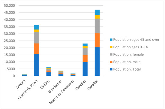
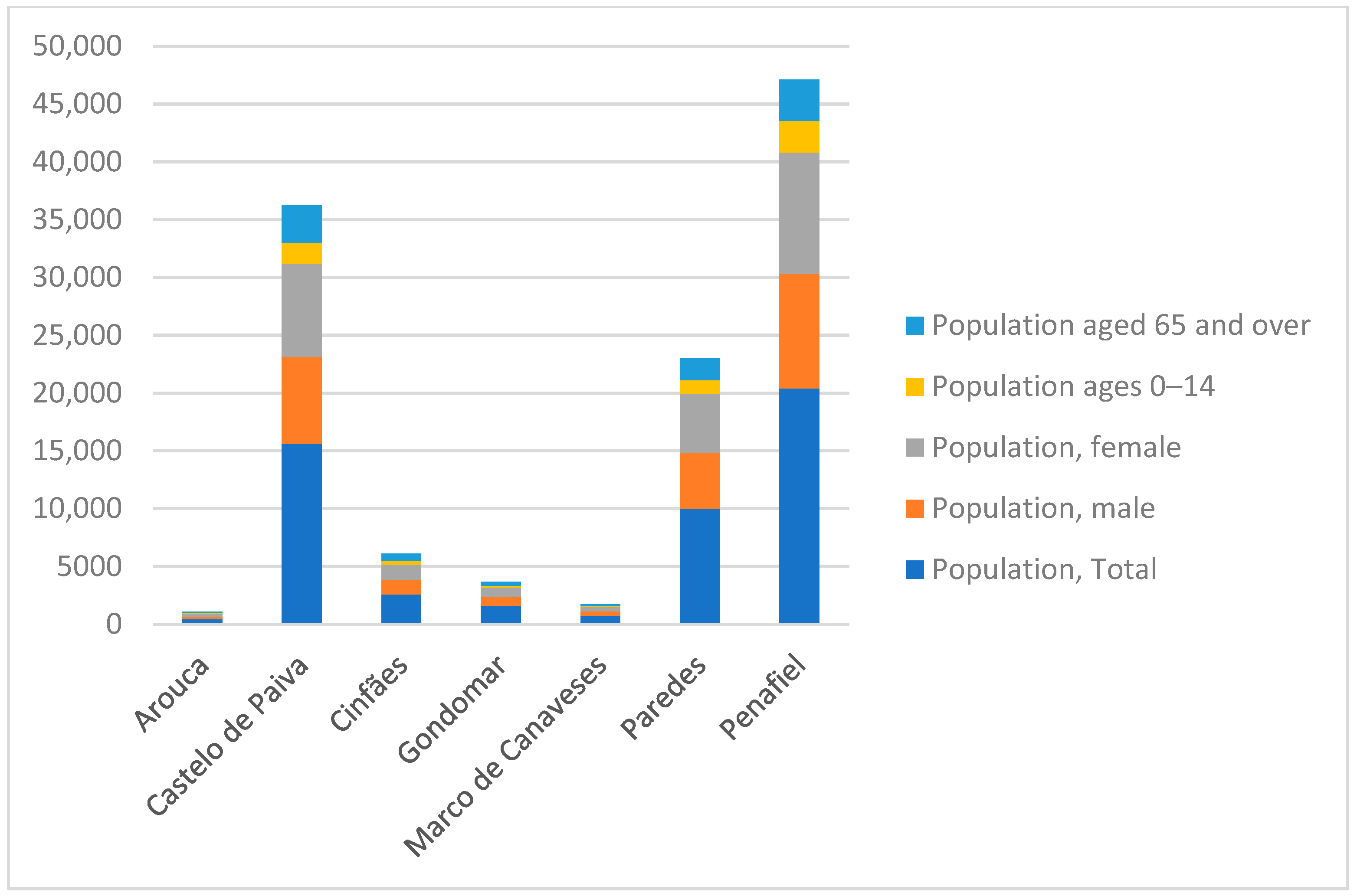
Using census data, we identified the number of individuals by district, civil parish, and census block. The study area includes seven districts, Arouca, Castelo de Paiva, Cinfães, Gondomar, Marco de Canaveses, Paredes, and Penafiel, and a total of 36 civil parishes. In total, 51,324 people live in the study area. Of these, 24,894 are male, representing 48.50 percent of the population, and 26,430 are female, representing 51.50 percent. Across both sexes, 6353 are children, representing 12.38 percent, and 9935 are aged 65 years and over, representing 19.36 percent (Figure 2).
Figure 2.
Population distribution by total number of the population, sex and age per district of the study area.
As shown, Penafiel is the most populous district, with 20,417 inhabitants. It also has the largest number of older adults, males, females, and children, followed by Castelo de Paiva. The least populous district is Arouca, with only 452 residents. These counts only represent the portions of each district within the study area, since the study area boundary does not coincide with district boundaries.
It is important to identify the characteristics of the populations of interest and their realistic spatial distribution to disaggregate and quantify the proportion of each group most likely to be exposed to wildfire risk.
3.1. Choropleth, Dasymetric, WUI, and Wildfire Forecast Maps
Only land-cover types that can actually have people living in them are considered in order to calculate the . In this case, water was excluded from this analysis. As expected, the of urbanized areas is the highest (Table 2); in this case, since building perimeters were combined with the LULC raster, we have two classes for inhabited areas such as buildings and urban areas. This was important, since both perimeters and buildings were considered in this analysis. Bare and shrubland classes have the lowest . It makes sense, since neither is part of an urban area; instead, they are part of the rural area.
Table 2.
Relative density results for the land-cover classes of the study area.
In this way, the raster was created, followed by the dasymetric maps. Normally, classes such as bare and shrubland would be assigned a value of 0; the LiDAR data for buildings was combined with LULC urban areas, and edifices were identified within these classes. To demonstrate the enhancement from building information derived from LiDAR data, the dasymetric method was also applied to the LULC map of the study area, excluding the “building” class. With this, the was also computed for the remaining classes (Table 3) using the same equations and methods mentioned above.
Table 3.
Relative density results for the land-cover classes without building information.
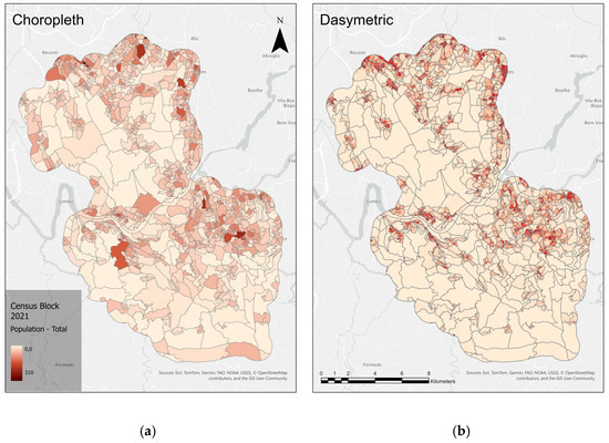
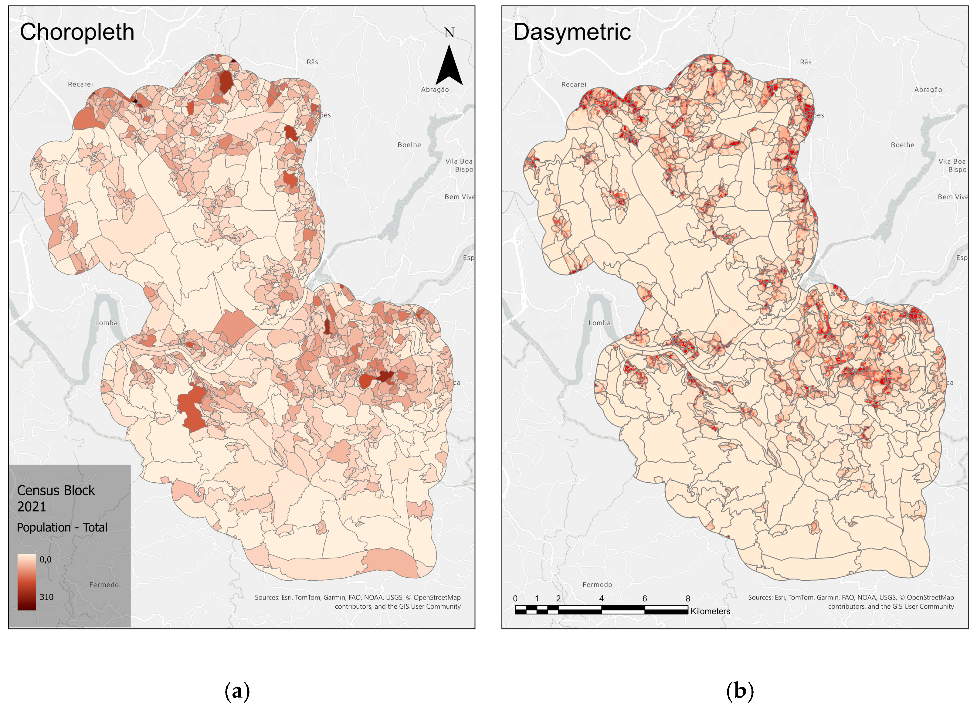
In addition to applying the dasymetric mapping methodology, dasymetric maps without LiDAR information and choropleth maps were created for comparison with the dasymetric maps to assess population density and distribution in the study area. Figure 3a shows the choropleth map of the total population by census block. As shown, the population is uniformly distributed across each block. In contrast, the dasymetric population map (Figure 3b) displays varying density classes within blocks, from lower to higher density areas, showing a more realistic distribution.
Figure 3.
Choropleth map of the total population (a) and dasymetric map of the total population (b).
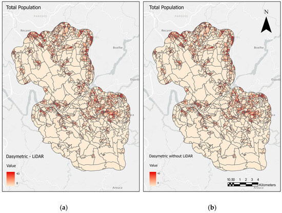
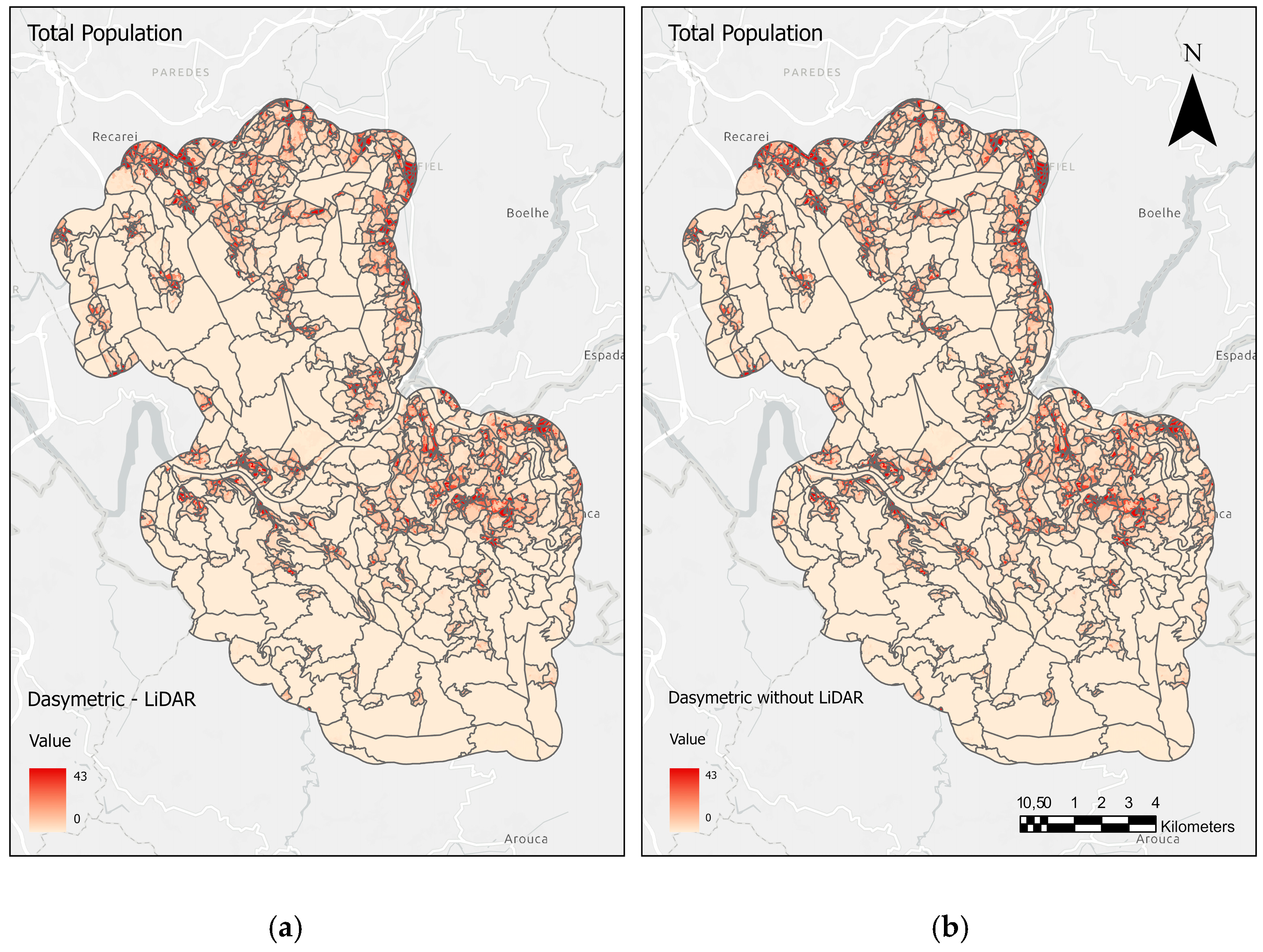
The same happened with the comparison between the dasymetric map of the study area with LiDAR information and without LiDAR information. The distribution of the total population is more dispersed throughout each census block with LiDAR information than with dasymetric maps without building information (Figure 4a,b). The dasymetric maps with and without building polygons are in Appendix A (Figure A1, Figure A2, Figure A3 and Figure A4).
Figure 4.
Dasymetric map of the total population with LiDAR building information (a) and dasymetric map of the total population without LiDAR building information (b).
When comparing the sum of the dasymetric results with the census block area using the Zonal Statistic tool, the method’s accuracy was demonstrated, as the population of both datasets was the same in all cases. This information is very important when decision-makers need to allocate resources to mitigate wildfire risk.
In Figure 4, the visual differences are almost imperceptible, but when comparing the rate and the percentage of the observed, expected, and headcount spatial information (Risk >= 3), there are significant differences among the values.
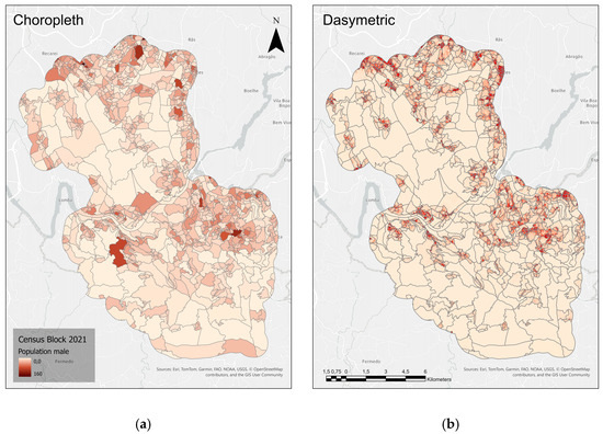
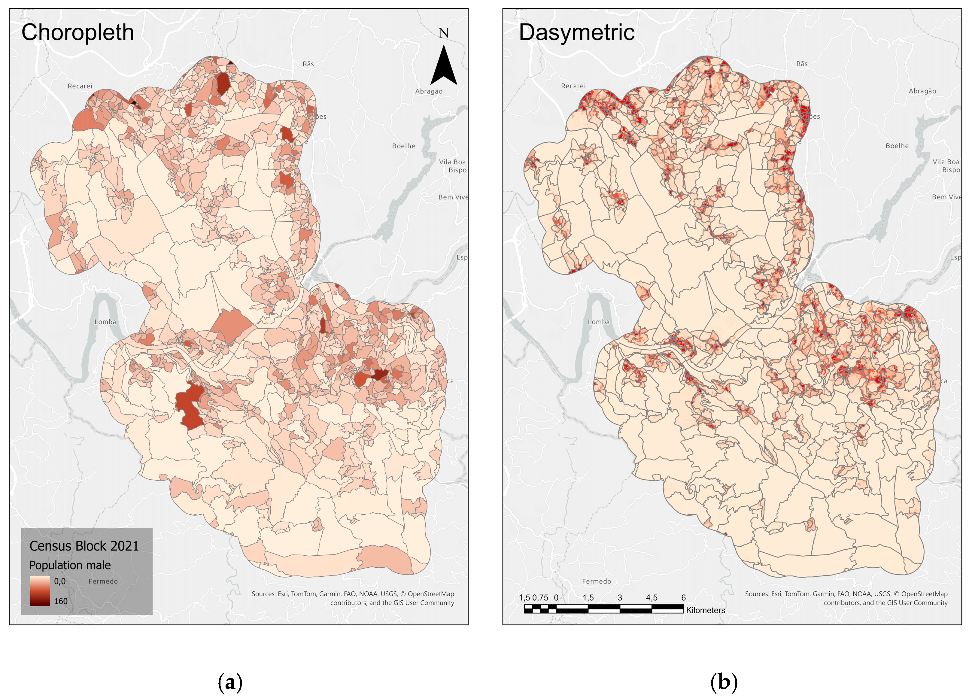
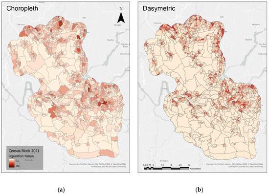
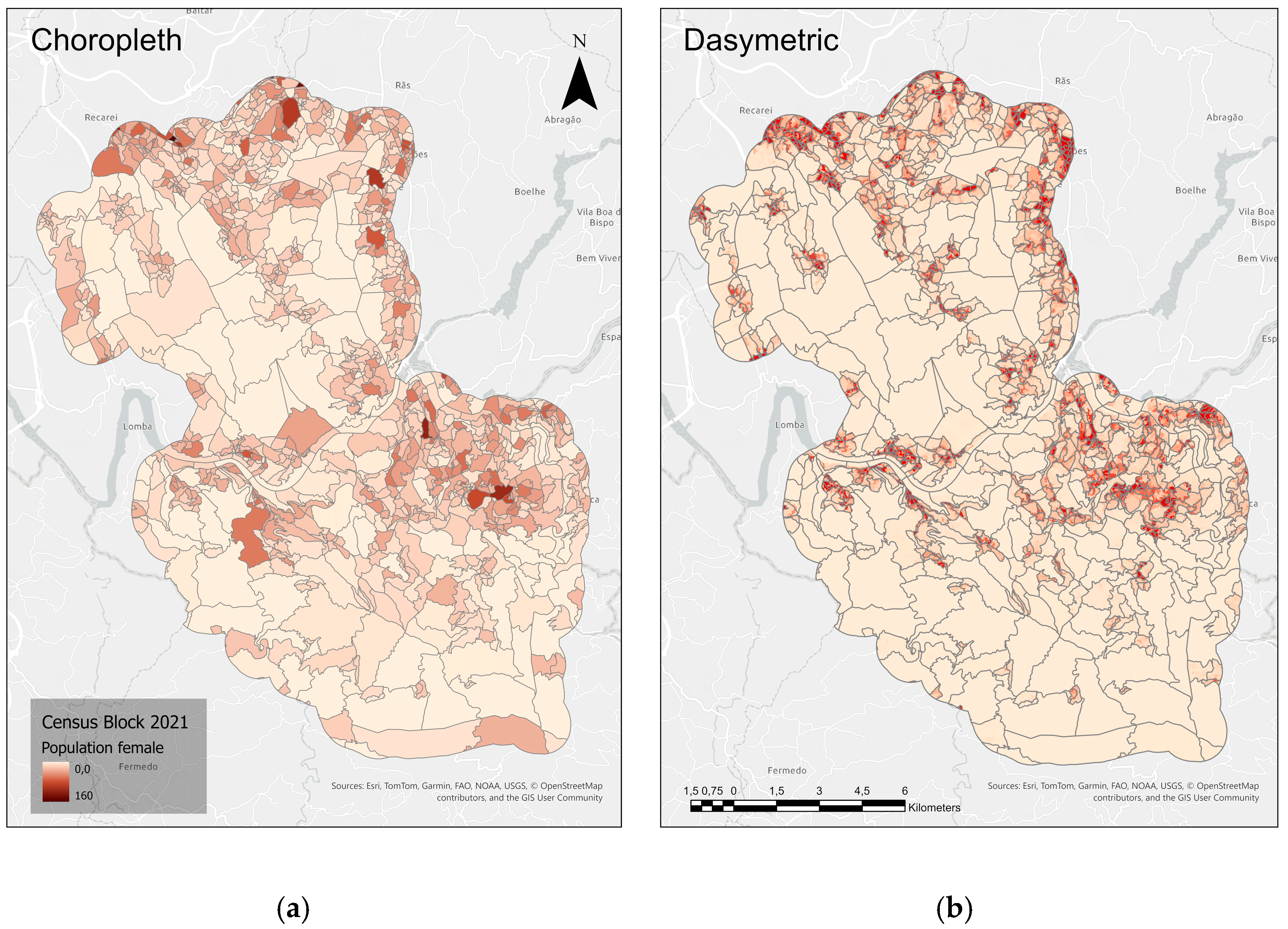
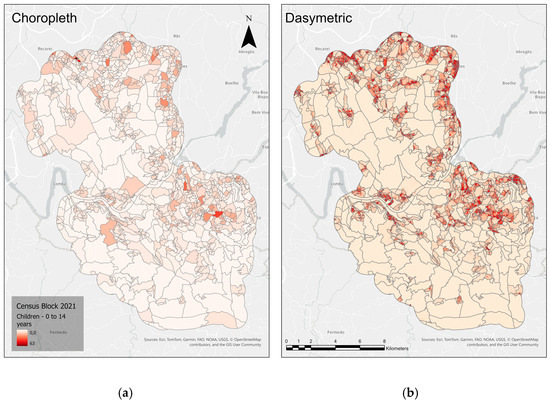
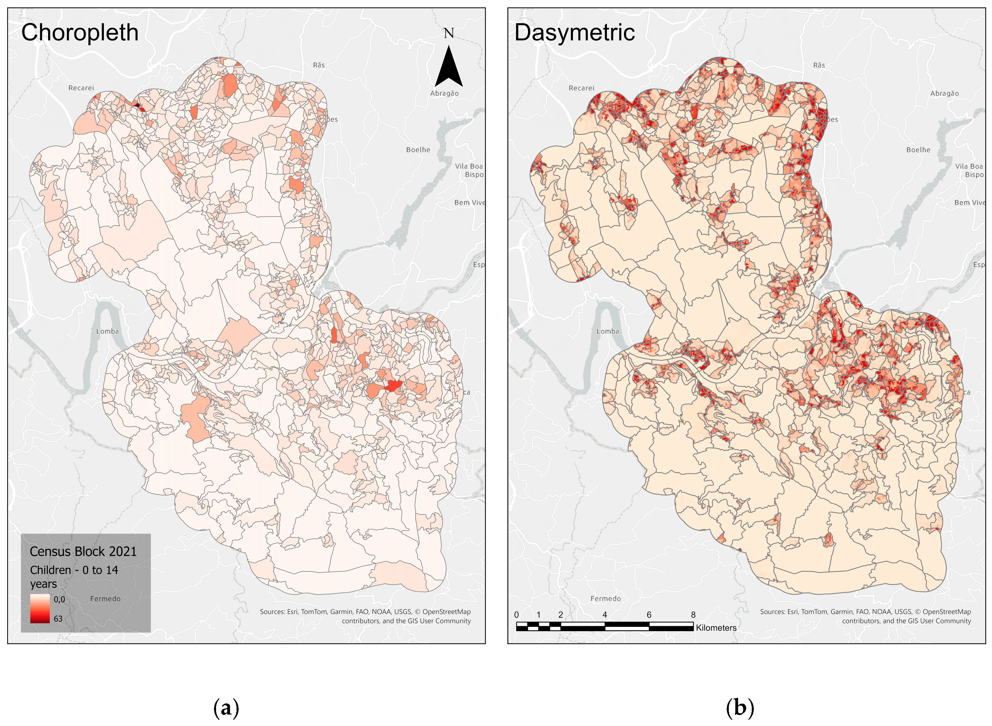
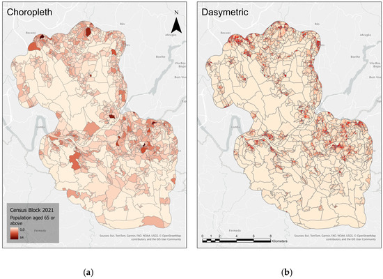
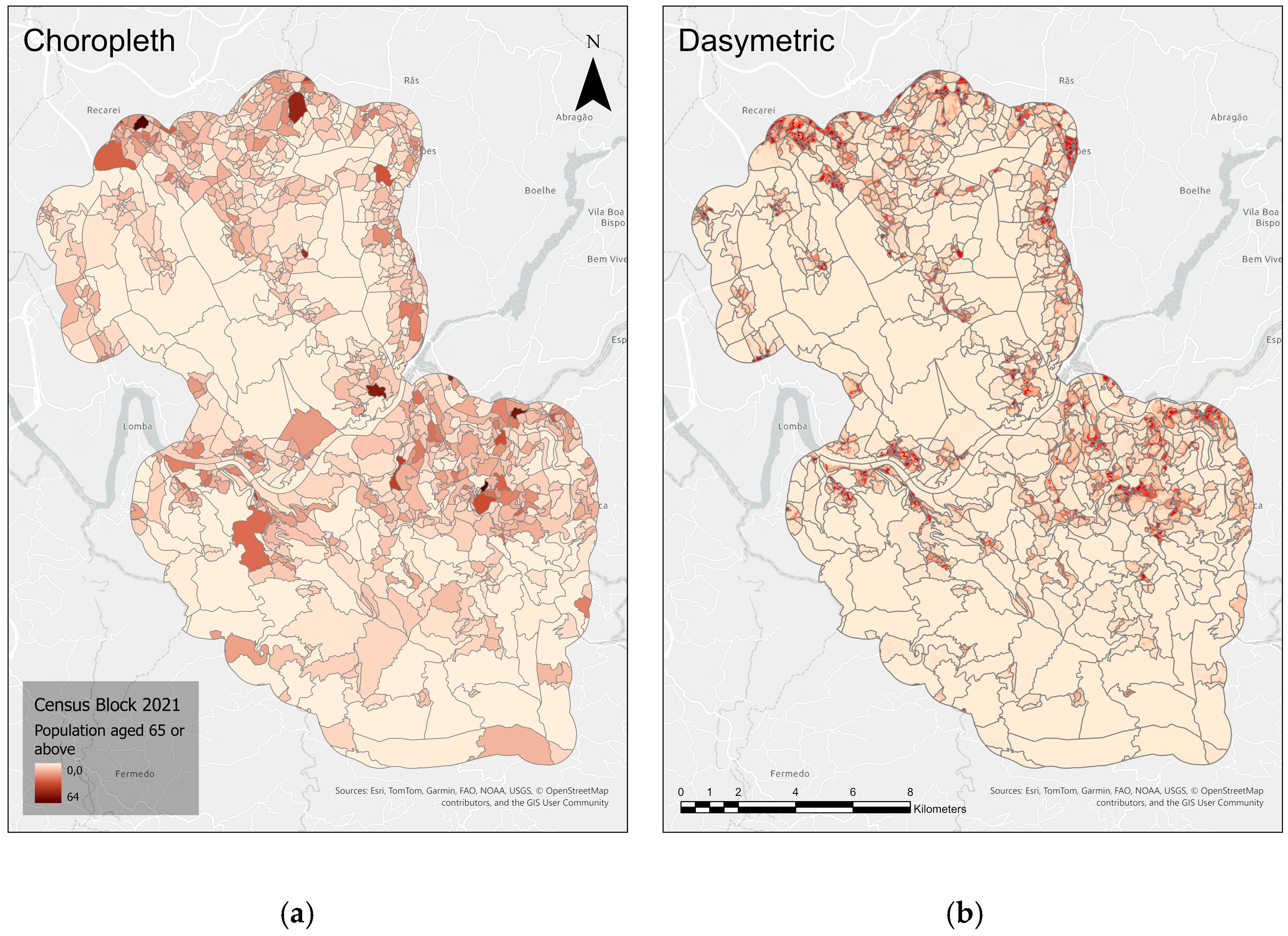
Following that, the choropleth maps of males (Figure 5a), females (Figure 6a), children (Figure 7a), and people aged 65 and above (Figure 8a) were elaborated. As can be seen, the dasymetric mapping methodology shows a better distribution of males (Figure 5b), females (Figure 6b), children (Figure 7b), and the elderly (Figure 8b).
Figure 5.
Choropleth map of male population (a), and dasymetric map of male population (b).
Figure 6.
Choropleth map of female population (a), and dasymetric map of female population (b).
Figure 7.
Choropleth map of child population, (a) and dasymetric map of child population (b).
Figure 8.
Choropleth map of population aged 65 or above population, (a) and dasymetric of map of population aged 65 or above population (b).
3.2. Expected Exposure, Observed Exposure, and Exposure to Risk
Expected exposure for each population subgroup was computed in ArcGIS Pro 3.4 using the Raster Calculator and Zonal Statistics. As noted above, only risk classes 3 or higher were considered, producing an expected exposure (headcount) map for each group.
The main advantage of the dasymetric method is that it reveals where populations are most likely at risk, making it easier to identify the most vulnerable residents, such as those living within the WUI. Moreover, it was possible to determine the number of residents within the WUI. Around 30,289 people live in this region, representing 59% of the study area’s population. It also highlights priority areas for allocating resources to reduce potential exposure and to implement other prevention measures. Notably, population information from choropleth maps is evenly distributed across census blocks; it would be impossible to visually identify densely populated areas or the number of inhabitants exposed.
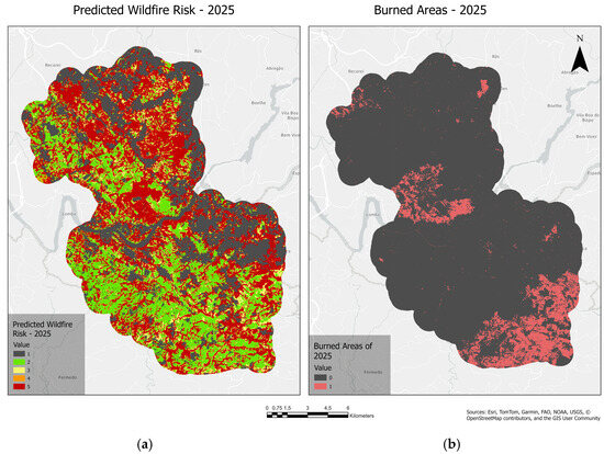
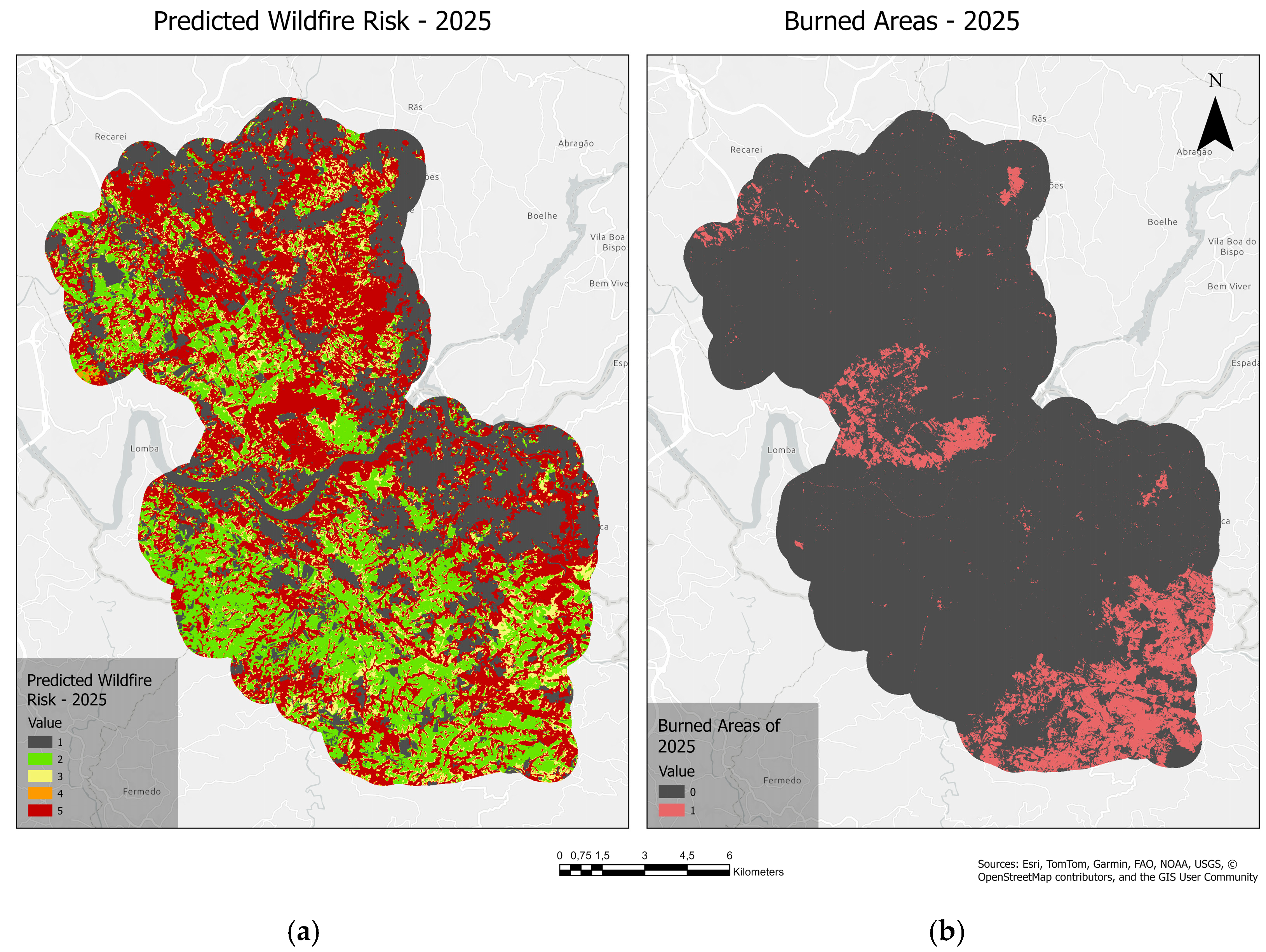
For observed exposure, the same workflow clearly identifies where the exposure was concentrated in 2025. We quantified the number of residents affected by the largest wildfires in the study area that year. Using the expected exposure maps, the predicted wildfire risk map (Figure 9), and the 2025 burned-area footprint, we calculated the expected exposure, predicted headcount at risk (risk class 3 or higher), and observed exposure for each population stratum (Table 4).
Figure 9.
Map of predicted wildfire risk for 2025 (a) and map of burned areas of 2025 derived from Sentinel-2 data (b).
Table 4.
Results of expected exposure: predicted headcount at risk and observed exposure of the AOI and WUI for total population and other groups of interest.
For the entire region, the expected number of people exposed to wildfires was approximately 1526. This estimate was derived from empirical burn probabilities. Expected exposure was computed by combining the 2025 burned footprint with each cell’s risk class to obtain a class-specific burn fraction, which was then applied to dasymetric population surfaces.
In contrast, the predicted headcount only used the 2025 wildfire risk map to quantify how many individuals in each population group could be at high risk of exposure. Because wildfires occurred in 2025, we also calculated the observed exposure by overlaying the burned area—derived from Sentinel-2 images and the vegetation index dNBR—with population maps, yielding the actual number of inhabitants exposed in 2025.
In addition, the percentages and rates of residents likely or actually exposed to wildfires were calculated for each variable and group listed in Table 5. The results are summarized in Table 5 below. On average, 3% of the total population was expected to be affected by wildfire across the entire study area, meaning that for every 100 inhabitants, about three would be affected. This is slightly higher than the rate inside the WUI, which is 2.7%. Although the percentage of people expected to be exposed is higher in the WUI (54%), this is because most people live in this region, and the metric is population weighted.
Table 5.
Rate and percentage of exposure for each population strata for the AOI and WUI.
A similar pattern appears for the predicted headcount at risk: the rate is higher for the entire area (25.3%) than inside the WUI (11.3%). Again, the percentage of exposure is higher inside the WUI (54.6%) than across the AOI (45.4%). On the other hand, when we look at the observed exposure, the rate is higher for the study area than for the WUI. The same holds for the percentage of the population exposed to wildfires: 76.7% of those exposed in 2025 lived outside the WUI. The main differences between the observed indicator and the expected and predicted indicators are that the observed indicator is empirical, whereas the others are model-derived. Most model-based metrics are probability-based, whereas the threshold headcount is a binary risk classification and is not probability weighted.
In 2025, the observed event shows that about 77% of affected residents lived outside of the WUI, whereas the model-based indicators suggest that, on average, about 54% of people potentially affected by future fires are within the WUI. This is not a contradiction, because a single wildfire is one realization of a stochastic process, and it is not possible to predict the exact cells that will burn. Wildfire occurrences are related to human activities, weather conditions, and land-cover type. These events are seen as the realization of a spatial–temporal process, which is a stochastic model for the occurrence of space and time events [37]. The observed metric describes what happened once, while the expected metrics describe where impacts are most likely to occur over time as a result of the simulation process.
The exposure rate and percentage for both dasymetric maps, with and without building polygons, were calculated.
When looking at the results in Table 5 and Table 6, a significant difference in rates and percentages between the population groups can be observed. Values computed from dasymetric maps without building polygons show increases in the rates and percentages of expected exposure for the total population, males, females, the elderly, and children. The most prominent difference between the two methods is shown in the predicted information of the child population. Although LULC, together with LiDAR building information, is used as a basis for creating the dasymetric map of the AOI, which demonstrates the possibility of children at risk (headcount) from wildfires in the WUI, the one without LiDAR data does not show any children at risk within the WUI.
Table 6.
Rate and percentage of exposure for each population strata for the AOI and WUI without LiDAR information.
It is worth mentioning that the rate increase and decrease are related to the different LULC classes. With LiDAR information, it was possible to map all residential buildings within the AOI and WUI due to its high resolution. While applying the dasymetric method, considering only LULC is not attainable. Due to the resolution of satellite imagery, urban areas become homogeneous, and features such as streets, squares, and other public spaces are not considered when calculating the RD of each class. As a consequence, there is an increase in the urban area’s RD value.
Therefore, the WUI remains a priority for preventive action, because it concentrates the expected exposure, but residents outside the WUI also warrant protective measures, since large events can still impact them, as they did in 2025. As noted, some groups can be slightly more impacted by these events than others. When we look at the observed indicator, children and females in the WUI were more affected in 2025 than males. Older adults were more affected outside the WUI than the other groups.
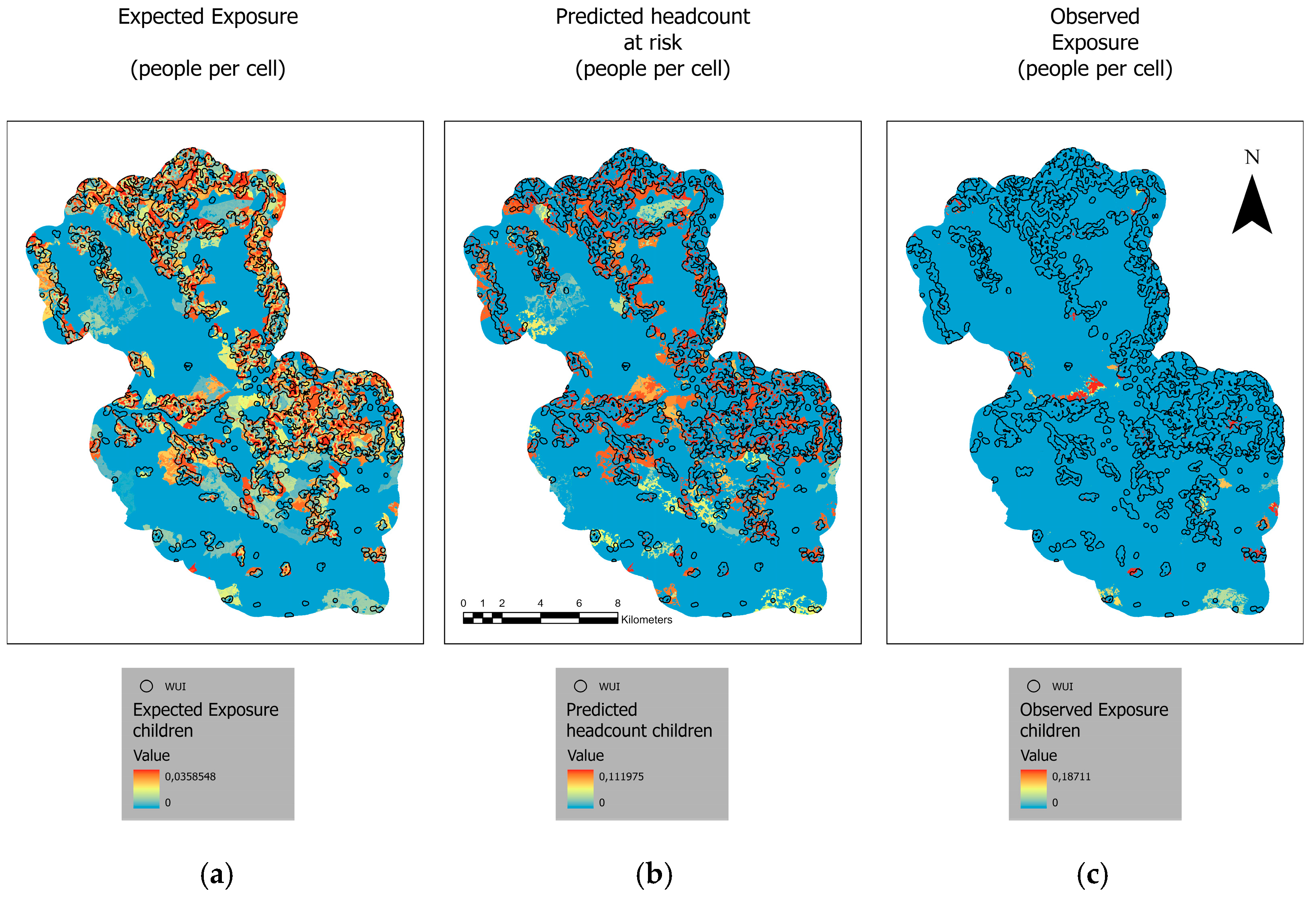
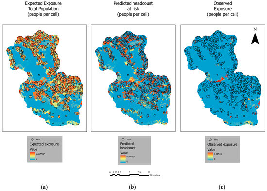
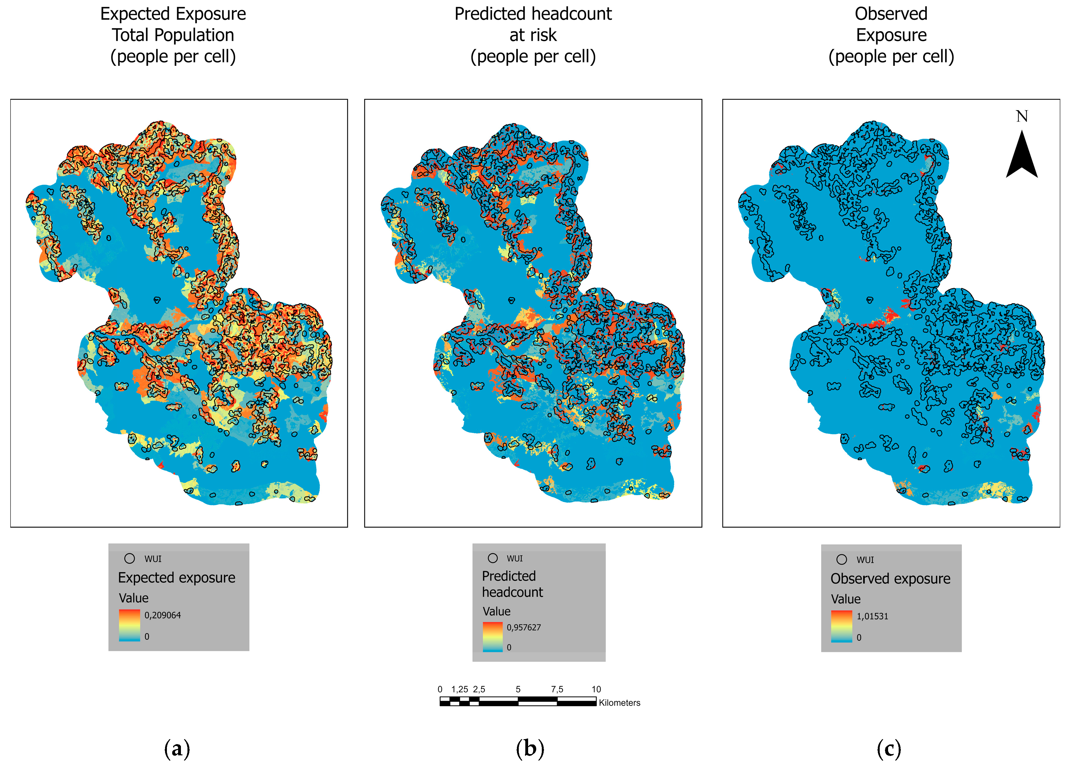
This can also be inferred from the maps prepared for each indicator and the statistical analysis of each population group. Figure 10 displays the maps for the total population, and maps for the other groups are in Appendix A (Figure A5, Figure A6, Figure A7 and Figure A8). It is clear that most people are possibly exposed at a higher risk within the WUI of the study area since most residents live there. Moreover, inhabitants outside the WUI are also affected by wildfire events, and these maps allow stakeholders to identify where measures should be implemented to reduce the expected population exposure to wildfire. This demonstrates that dasymetric maps have the potential to serve as an auxiliary tool for anticipating and mitigating the impacts on people who may be exposed to wildfires.
Figure 10.
Map of the expected exposure (a), predicted headcount at risk (b), and observed exposure (c) for the total population of the entire study area and WUI.
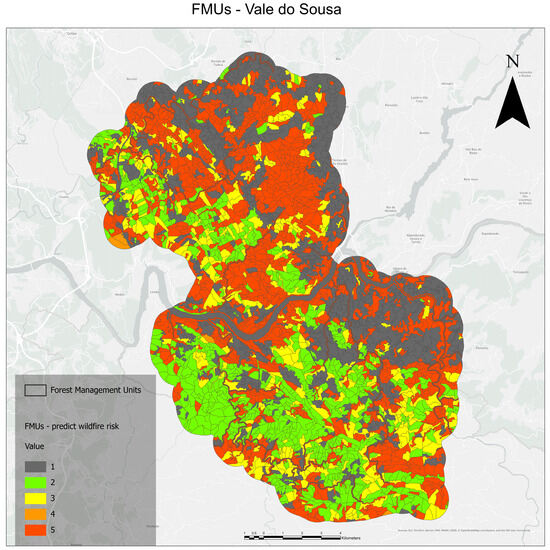
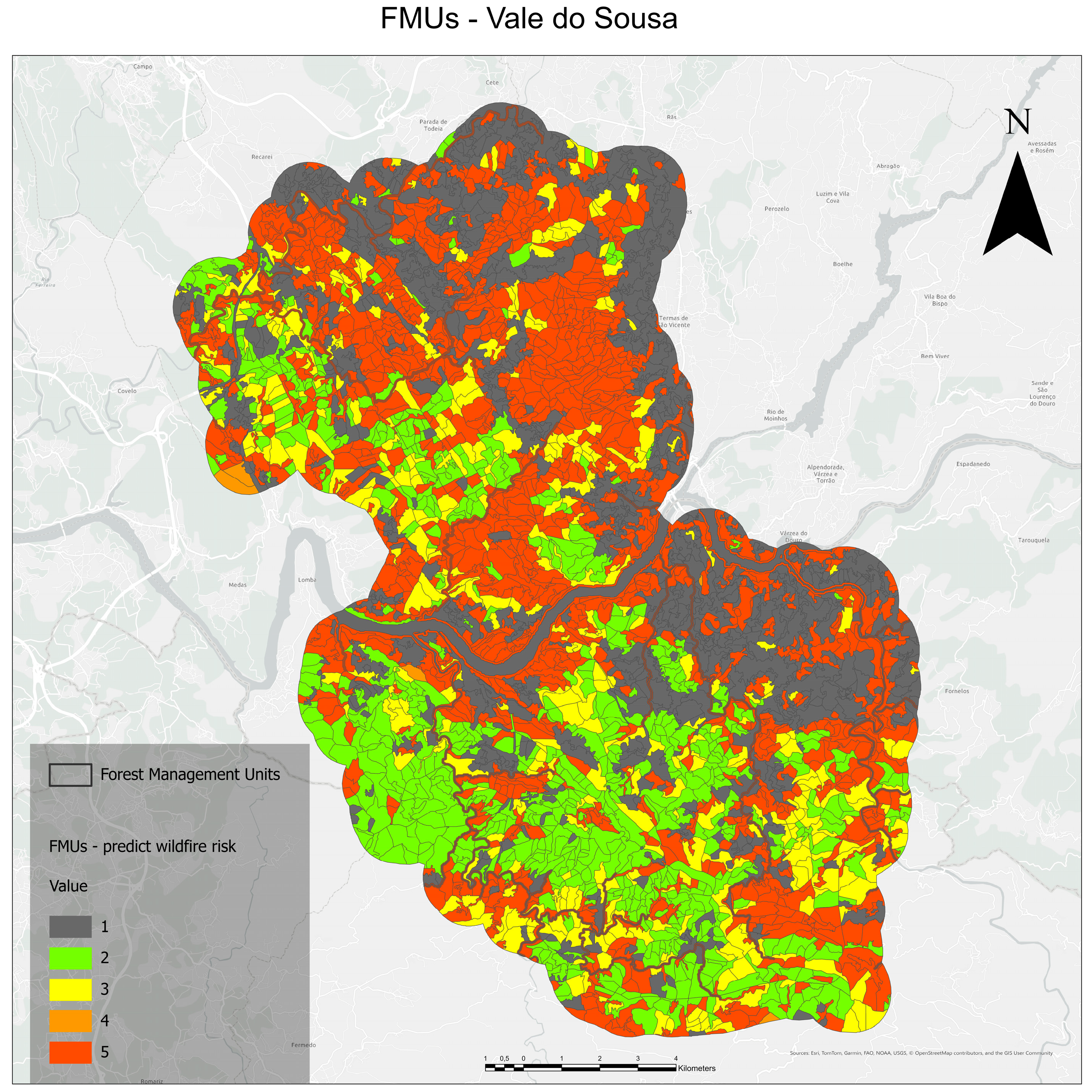
In this manner, the FMUs possibly exposed to wildfires were also mapped. Class 1 is classified as very-low risk and encompasses areas such as dense residential areas, agricultural lands, water bodies, bare lands, and sparse buildings. Class 2 is low to moderate; class 3 is moderate to high; class 4 is high to very high; and class 5 is very high to extremely high. The same classification was applied to develop the predicted wildfire risk map, where 27% of the area was classified as class 1, 21.7% as class 2, 13.4% as class 3, 1% as class 4, and around 36% of the FMUs as class 5 (Figure 11). This information is important to refine even more where the areas should be prioritized inside the WUI and the FMUs when overlapping this information with the population maps, making it possible to allocate resources in a more effective way in order to protect the residents and manage the forested land efficiently.
Figure 11.
Map of FMUs with risk classification: class 1: very low; class 2: low to moderate; class 3: moderate to high; class 4: high to very high; and class 5: very high to extremely high.
Furthermore, the proposed disaggregation method could be applied to other areas due to its high accuracy and other ancillary information that can be correlated with the population information. In Liu et al., [25] due to the lack of population distribution data and low spatial resolution of the remote sensing nighttime light (NTL), they used the light data from the SDGSAT-1 satellite and the population distribution information from WorldPop (100 m grid resolution), which was disaggregated to a high resolution of 10 m × 10 m.
In this manner, the possible limitation of this method is related to the lack of high-resolution data, inaccuracy in LULC classification, and the absence of information about the population of the area of interest. This could lead to an overestimation or an underestimation of the estimated population. Thus, LiDAR building footprints played an important role in improving the methodology, given their high spatial resolution. Because of LiDAR surveying costs, it is not always possible to have this type of information; consequently, the spatial data resolution would be conditioned on the availability of open spatial data with high spatial resolution.
4. Conclusions
Choropleth maps are widely used to examine population distribution across regions. However, because they allocate population counts uniformly across entire census blocks, they obscure fine-scale density patterns and can hinder decision-making by making it harder to pinpoint where the population is truly concentrated. By contrast, disaggregating census data into smaller cells makes it possible to visualize denser pockets within the same blocks, i.e., where population strata are actually concentrated. Although the application of this method is complex and sometimes it can be a challenge, when compared to the choropleth method, the distribution of the population is more realistic. In this study, we disaggregated census data using a dasymetric method into 10 m × 10 m cells, which clarifies intra-block variation and facilitates the identification of areas and population groups that are more exposed to wildfires within the study area, including within the WUI.
Risk was computed predictively by applying a ConvRNN to forecast future fires prior to this year’s wildfire events. Expected exposure was then estimated empirically using observed burned-area footprints within the study area. In 2025, approximately 77% of inhabitants exposed to wildfires lived outside the WUI, while the expected population exposure model suggested that 54% of the population affected by wildfires lived inside the WUI. However, wildfire events are the realization of one spatial–temporal process that could or could not happen in the same location, while the simulation shows where these events are most likely to occur. Importantly, the dasymetric surface reconciles with block-level population totals, and residential structure locations derived from LiDAR corroborate the spatial plausibility of exposure patterns. It is worth mentioning that the pycnophylactic property of the data must be preserved, and depending on the dataset available, due to the spatial resolution, which could not take into account the sparsely inhabited areas, this could impact this property. In this study, this did not occur, because the applied methodology preserved it, enhanced by the LiDAR data. Integrating these layers at the cell level enabled per-cell identification of potential population exposure across the area of interest and supported the assessment of where people are more likely to face a higher risk. Furthermore, quantitative validation and error diagnostics are reported in the ConvRNN study on wildfire forecasting.
These results show that combining 10 m dasymetric disaggregation with ConvRNN-based predictive risk mapping provides actionable, higher-resolution decision support for risk reduction, forest management, and spatial planning. Higher-resolution products reveal exposure hotspots and reduce spatial uncertainty relative to choropleth maps, enabling stakeholders to prioritize interventions and allocate scarce resources more efficiently, especially for vulnerable groups such as older adults and children in the WUI, while not neglecting residents outside it. Remaining uncertainties are related to ancillary data assumptions in dasymetric disaggregation and model generalization in forecasting, but the approach is immediately applicable to operational decision-making in Vale do Sousa and other areas of interest.
Author Contributions
Conceptualization, B.P.-B. and A.C.T.; Methodology, B.P.-B., J.G.B., S.M. and A.C.T.; Software, B.P.-B.; Formal analysis, B.P.-B.; Writing—original draft, B.P.-B.; Writing—review and editing, B.P.-B., J.G.B., S.M. and A.C.T. All authors have read and agreed to the published version of the manuscript.
Funding
Bárbara Pavani-Biju was financially supported by Portuguese national funds through the Foundation for Science and Technology I.P. (grant reference number: 2022. 13033.BD) and Decision Support for the Supply of Ecosystem Services under Global Change (DecisionES) (grant agreement number: 101007950—H2020-MSCA-RISE-2020). José G. Borges and Susete Marques were financially supported by Portuguese national funds through the Foundation for Science and Technology I.P. of the Forest Research Centre and DOI identifier UID/00239/2025 (DOI: 10.54499/UID/00239/2025). The authors acknowledge the financial support provided to the Institute of Earth Sciences (ICT) through the multi-annual funding contract with the Foundation for Science and Technology (FCT), under project UID/04683/2025 with the DOI https://doi.org/10.54499/UID/04683/2025.
Data Availability Statement
The datasets presented in this article are not readily available because the data are part of an ongoing study. Requests to access the datasets should be directed to up201700360@edu.fc.up.pt.
Acknowledgments
The first author would like to thank Ricardo Paludzyszyn and Thomas Callewaert who provided support during the development of this paper. During the preparation of this manuscript, the authors used DeepSeek (version DeepSeek-V3) for the purposes of improving language fluency and review. The authors have reviewed and edited the output and take full responsibility for the content of this publication.
Conflicts of Interest
The authors declare no conflicts of interest.
Appendix A
Figure A1.
Map of male population with LiDAR information (a), and map of male population without LiDAR information (b).
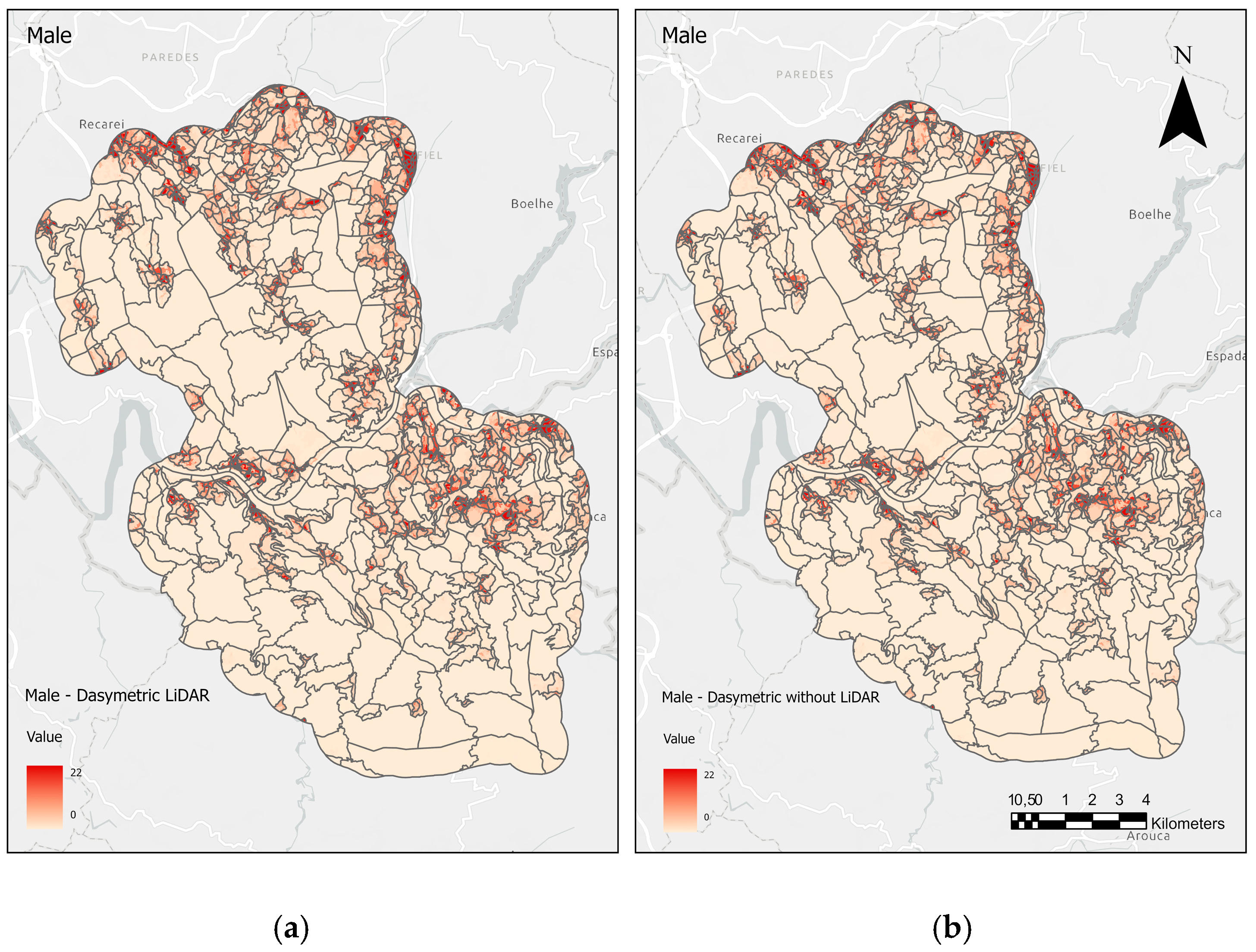
Figure A2.
Map of female population with LiDAR information (a), and map of female population without LiDAR information (b).
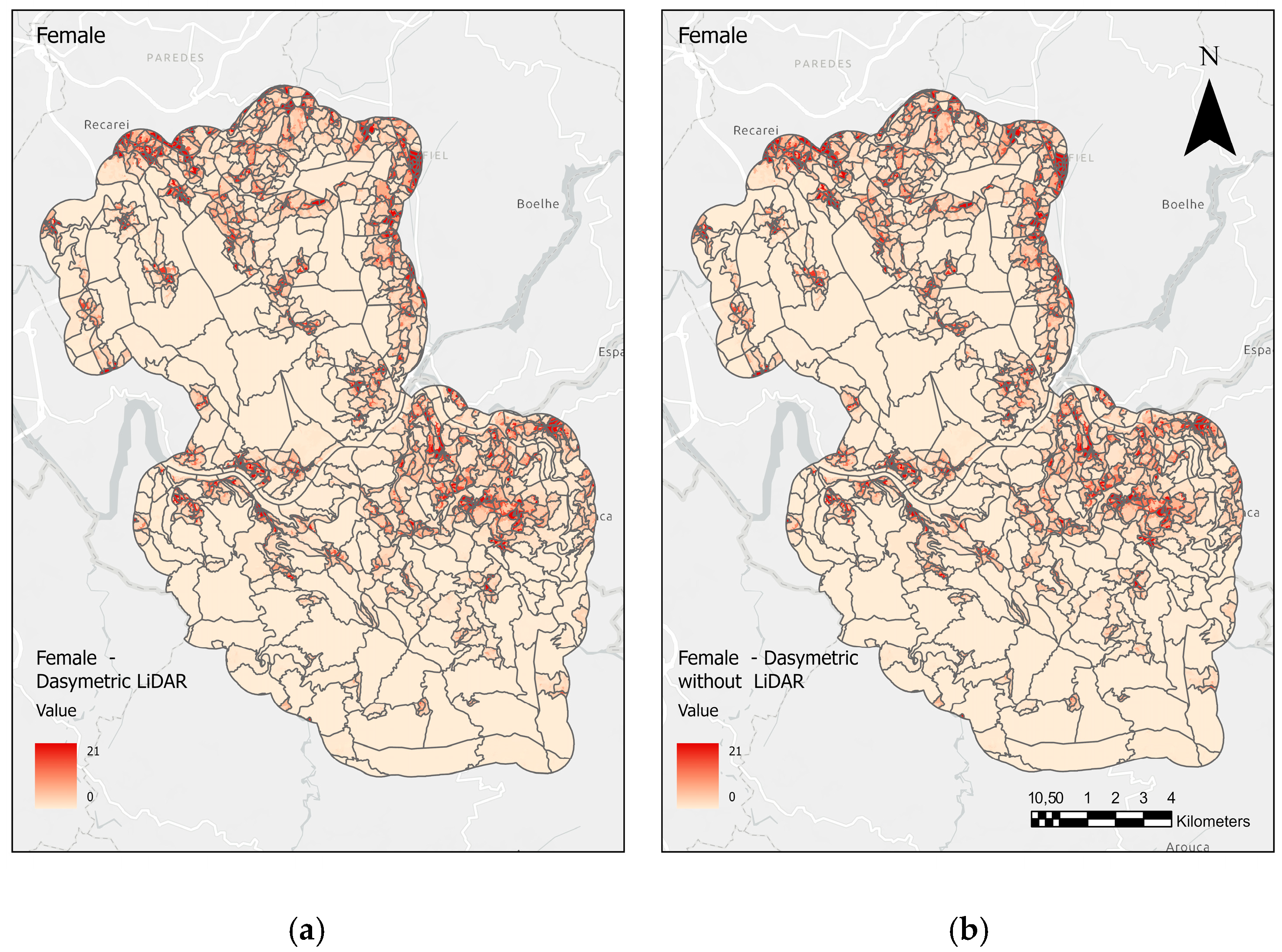
Figure A3.
Map of elderly population with LiDAR information (a), and map of elderly population without LiDAR information (b).
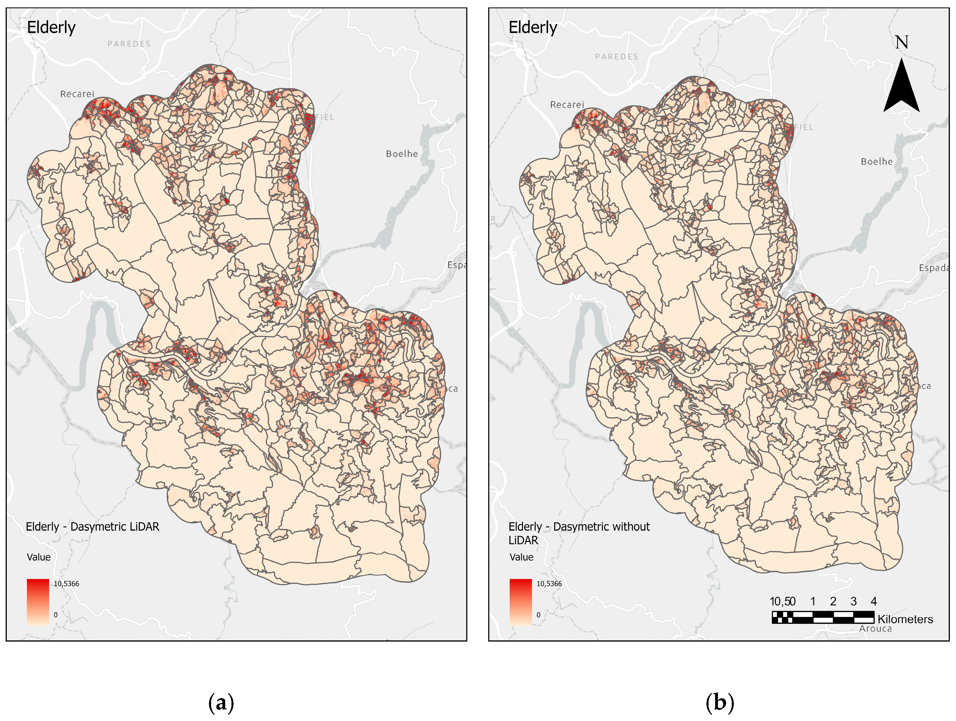
Figure A4.
Map of Children population with LiDAR information (a), and map of Children population without LiDAR information (b).
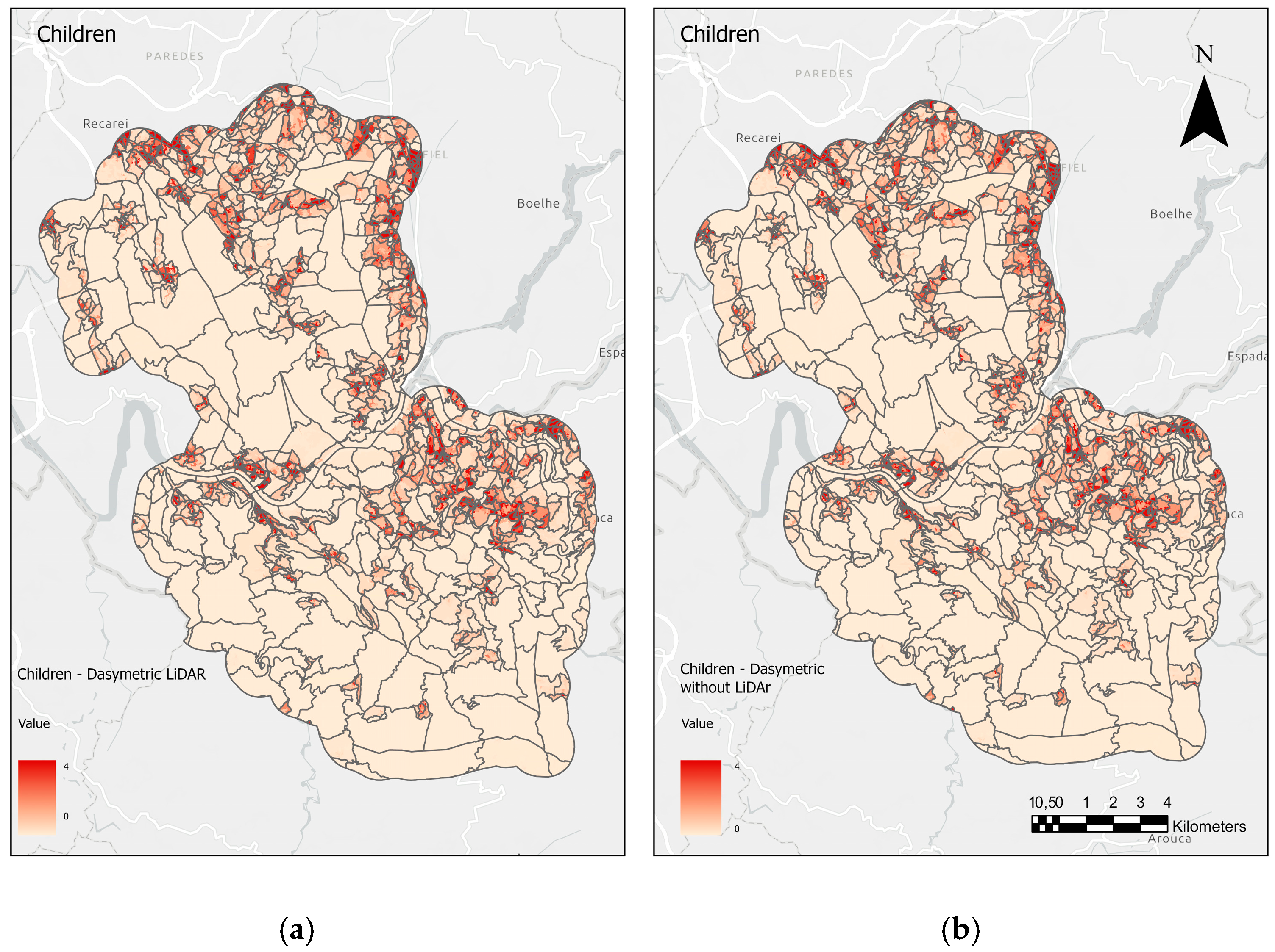
Figure A5.
Map of the expected exposure (a), predicted headcount at risk (b), and observed exposure (c) for the female population of the entire study area and WUI.
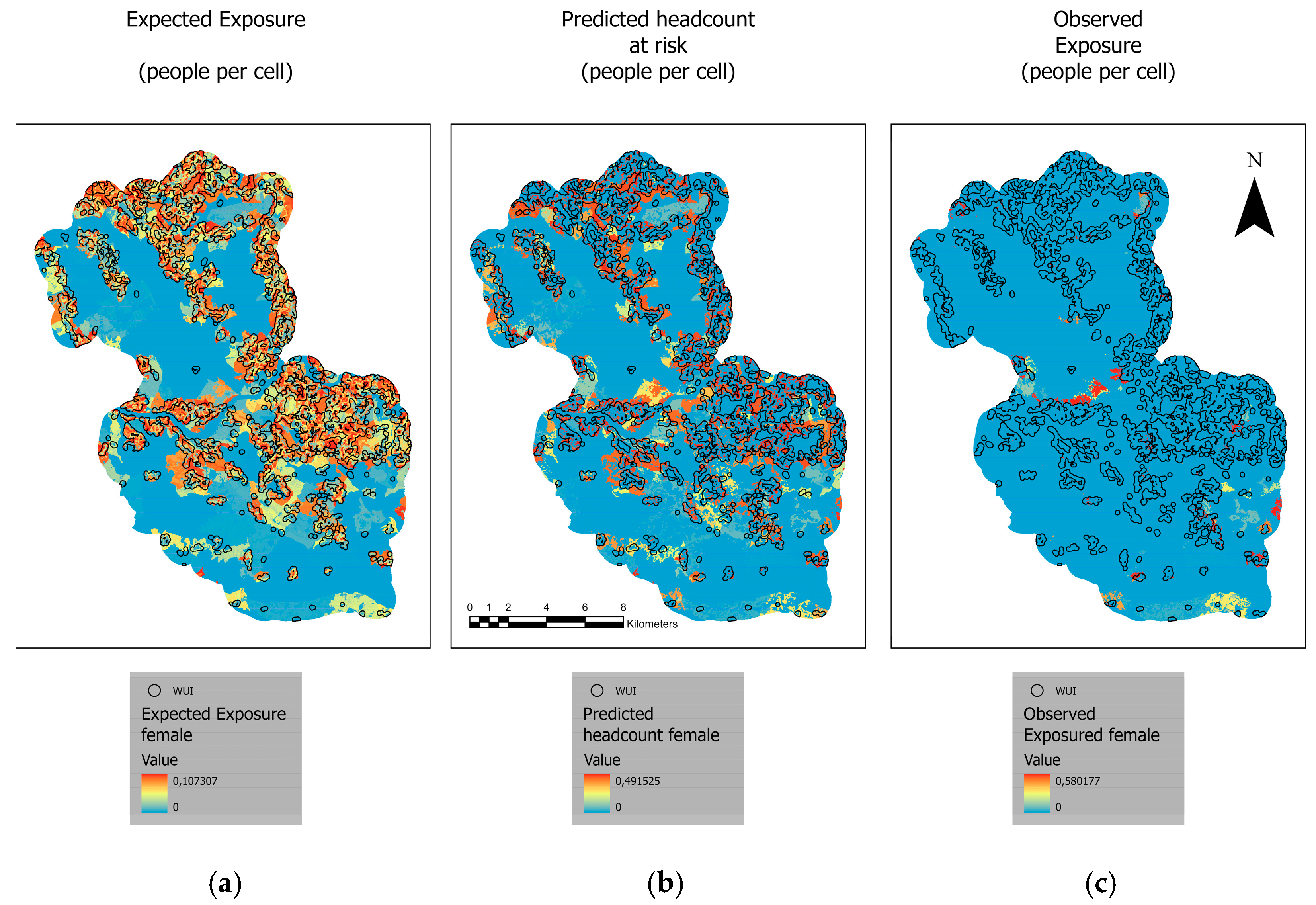
Figure A6.
Map of the expected exposure (a), predicted headcount at risk (b), and observed exposure (c) for the male population of the entire study area and WUI.
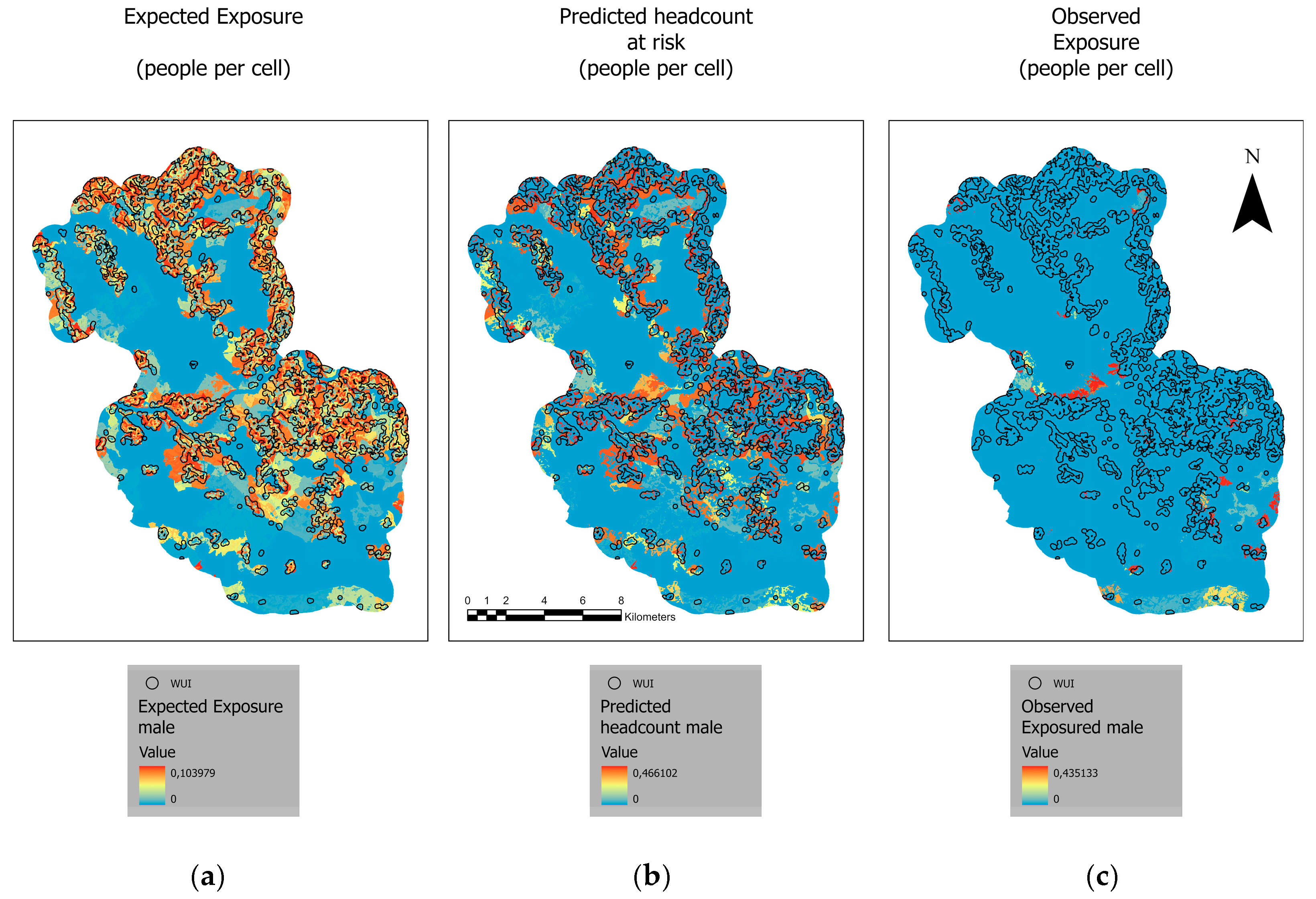
Figure A7.
Map of the expected exposure (a), predicted headcount at risk (b), and observed exposure (c) for the elderly population of the entire study area and WUI.
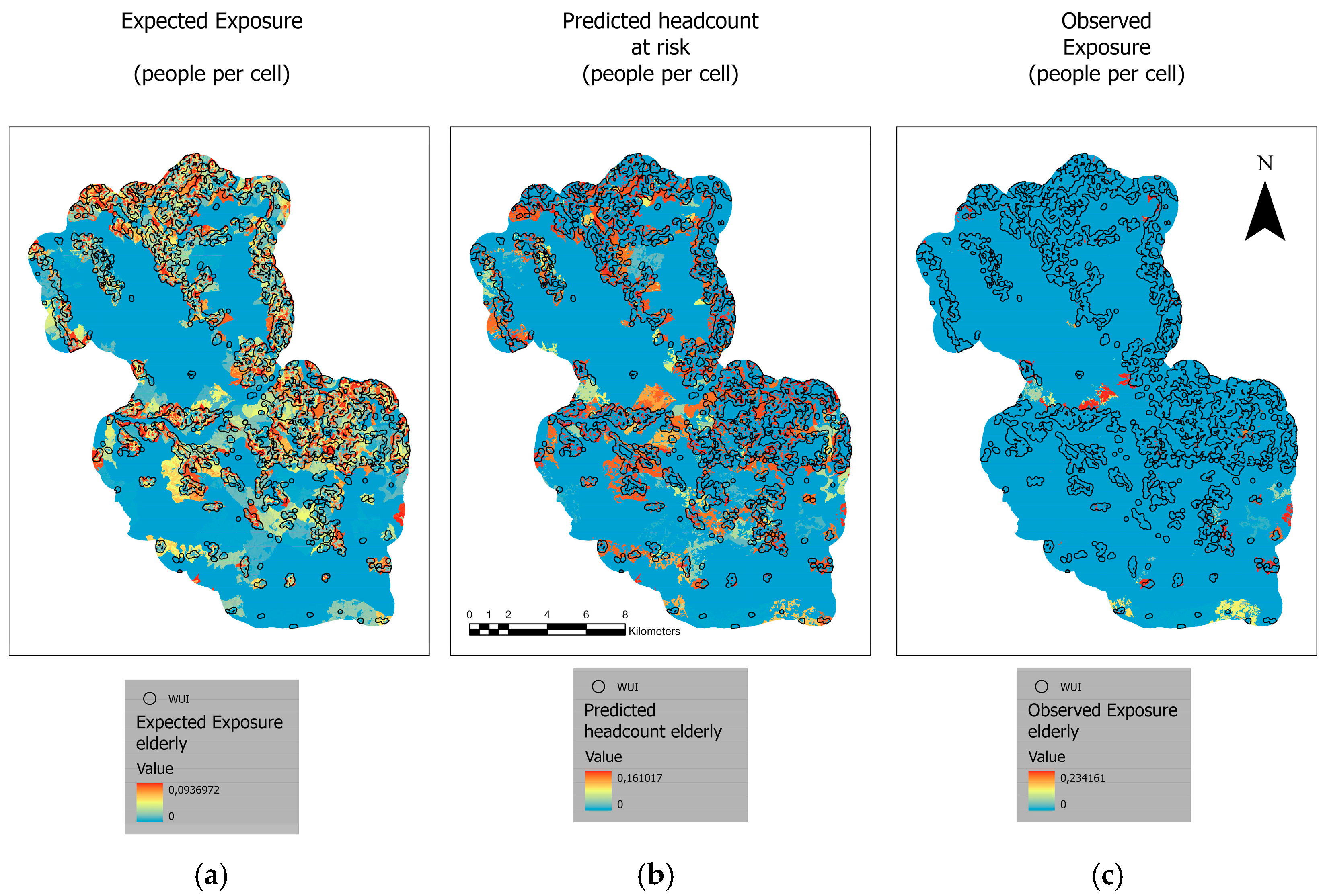
Figure A8.
Map of the expected exposure (a), predicted headcount at risk (b), and observed exposure (c) for the child population of the entire study area and WUI.
References
- Meier, S.; Elliott, R.J.R.; Strobl, E. The Regional Economic Impact of Wildfires: Evidence from Southern Europe. J. Environ. Econ. Manag. 2023, 118, 102787. [Google Scholar] [CrossRef] [Scilit]
- Calviño-Cancela, M.; Chas-Amil, M.L.; García-Martínez, E.D.; Touza, J. Interacting Effects of Topography, Vegetation, Human Activities and Wildland-Urban Interfaces on Wildfire Ignition Risk. For. Ecol. Manag. 2017, 397, 10–17. [Google Scholar] [CrossRef] [Scilit]
- Radeloff, V.C.; Helmers, D.P.; Anu Kramer, H.; Mockrin, M.H.; Alexandre, P.M.; Bar-Massada, A.; Butsic, V.; Hawbaker, T.J.; Martinuzzi, S.; Syphard, A.D.; et al. Rapid Growth of the US Wildland-Urban Interface Raises Wildfire Risk. Proc. Natl. Acad. Sci. USA 2018, 115, 3314–3319. [Google Scholar] [CrossRef] [Scilit] [PubMed]
- Argañaraz, J.P.; Radeloff, V.C.; Bar-Massada, A.; Gavier-Pizarro, G.I.; Scavuzzo, C.M.; Bellis, L.M. Assessing Wildfire Exposure in the Wildland-Urban Interface Area of the Mountains of Central Argentina. J. Environ. Manag. 2017, 196, 499–510. [Google Scholar] [CrossRef] [Scilit] [PubMed]
- Modugno, S.; Balzter, H.; Cole, B.; Borrelli, P. Mapping Regional Patterns of Large Forest Fires in Wildland-Urban Interface Areas in Europe. J. Environ. Manag. 2016, 172, 112–126. [Google Scholar] [CrossRef] [Scilit]
- Pereira, J.M.C.; Alexandre, P.M.; Campagnolo, M.L.; Bar-Massada, A.; Radeloff, V.C.; Silva, P.C. Defining and Mapping the Wildland-Urban Interface in Portugal. In Advances in Forest Fire Research 2018; Imprensa da Universidade de Coimbra: Coimbra, Portugal, 2018; pp. 742–749. [Google Scholar]
- Chas-Amil, M.L.; Nogueira-Moure, E.; Prestemon, J.P.; Touza, J. Spatial Patterns of Social Vulnerability in Relation to Wildfire Risk and Wildland-Urban Interface Presence. Landsc. Urban Plan. 2022, 228, 104577. [Google Scholar] [CrossRef] [Scilit]
- Schug, F.; Bar-Massada, A.; Carlson, A.R.; Cox, H.; Hawbaker, T.J.; Helmers, D.; Hostert, P.; Kaim, D.; Kasraee, N.K.; Martinuzzi, S.; et al. The Global Wildland–Urban Interface. Nature 2023, 621, 94–99. [Google Scholar] [CrossRef] [Scilit]
- Hanberry, B.B. Reclassifying the Wildland-Urban Interface Using Fire Occurrences for the United States. Land 2020, 9, 225. [Google Scholar] [CrossRef] [Scilit]
- Badia, A.; Pallares-Barbera, M.; Valldeperas, N.; Gisbert, M. Wildfires in the Wildland-Urban Interface in Catalonia: Vulnerability Analysis Based on Land Use and Land Cover Change. Sci. Total Environ. 2019, 673, 184–196. [Google Scholar] [CrossRef] [Scilit]
- Parente, J.; Pereira, M.G.; Amraoui, M.; Tedim, F. Negligent and Intentional Fires in Portugal: Spatial Distribution Characterization. Sci. Total Environ. 2018, 624, 424–437. [Google Scholar] [CrossRef] [Scilit]
- ESA Copernicus Data Space Ecosystem Browser. Available online: https://browser.dataspace.copernicus.eu/ (accessed on 5 November 2024).
- Xu, Z.; Li, J.; Cheng, S.; Rui, X.; Zhao, Y.; He, H.; Guan, H.; Sharma, A.; Erxleben, M.; Chang, R.; et al. Deep Learning for Wildfire Risk Prediction: Integrating Remote Sensing and Environmental Data. ISPRS J. Photogramm. Remote Sens. 2025, 227, 632–677. [Google Scholar] [CrossRef] [Scilit]
- Uehara, T.D.T.; Körting, T.S.; Soares, A.d.R.; Quevedo, R.P. Time-Series Metrics Applied to Land Use and Land Cover Mapping with Focus on Landslide Detection. J. Appl. Remote Sens. 2022, 16, 034518. [Google Scholar] [CrossRef] [Scilit]
- Wulder, M.A.; Bater, C.W.; Coops, N.C.; Hilker, T.; White, J.C. The Role of LiDAR in Sustainable Forest Management. For. Chron. 2008, 84, 807–826. [Google Scholar] [CrossRef] [Scilit]
- Nunes, A.N.; Figueiredo, A.; Pinto, C.; Lourenço, L. Assessing Wildfire Hazard in the Wildland–Urban Interfaces (WUIs) of Central Portugal. Forests 2023, 14, 1106. [Google Scholar] [CrossRef] [Scilit]
- Tarsha Kurdi, F.; Lewandowicz, E.; Gharineiat, Z.; Shan, J. High-Resolution Building Indicator Mapping Using Airborne LiDAR Data. Electronics 2025, 14, 1821. [Google Scholar] [CrossRef] [Scilit]
- Han, S.Y.; Rey, S.; Knaap, E.; Kang, W.; Wolf, L. Adaptive Choropleth Mapper: An Open-Source Web-Based Tool for Synchronous Exploration of Multiple Variables at Multiple Spatial Extents. ISPRS Int. J. Geo-Inf. 2019, 8, 509. [Google Scholar] [CrossRef] [Scilit]
- Bonnevie, I.M.; Hansen, H.S.; Schrøder, L. Dasymetric Algorithms Using Land Cover to Estimate Human Population at Smaller Spatial Scales. ISPRS Int. J. Geo-Inf. 2024, 13, 427. [Google Scholar] [CrossRef] [Scilit]
- Reiter, D.; Jehling, M.; Hecht, R. Benefits of Using Address-Based Dasymetric Mapping in Micro-Level Census Disaggregation. AGILE GISci. Ser. 2023, 4, 38. [Google Scholar] [CrossRef] [Scilit]
- Monteiro, J.; Martins, B.; Murrieta-Flores, P.; Pires, J.M. Spatial Disaggregation of Historical Census Data Leveraging Multiple Sources of Ancillary Information. ISPRS Int. J. Geo-Inf. 2019, 8, 327. [Google Scholar] [CrossRef] [Scilit]
- Pirowski, T.; Szypuła, B. Dasymetric Population Mapping Using Building Data. Ann. Am. Assoc. Geogr. 2024, 114, 1001–1019. [Google Scholar] [CrossRef] [Scilit]
- Cartagena-Colón, M.; Mattei, H.; Wang, C. Dasymetric Mapping of Population Using Land Cover Data in JBNERR, Puerto Rico during 1990–2010. Land 2022, 11, 2301. [Google Scholar] [CrossRef] [Scilit]
- Mennis, J. Generating Surface Models of Population Using Dasymetric Mapping. Prof. Geogr. 2003, 55, 31–42. [Google Scholar] [CrossRef] [Scilit]
- Liu, C.; Chen, Y.; Wei, Y.; Chen, F. Spatial Population Distribution Data Disaggregation Based on SDGSAT-1 Nighttime Light and Land Use Data Using Guilin, China, as an Example. Remote Sens. 2023, 15, 2926. [Google Scholar] [CrossRef] [Scilit]
- Pascual, A.; Tóth, S.F. Using Mixed Integer Programming and Airborne Laser Scanning to Generate Forest Management Units. J. For. Res. 2022, 33, 217–226. [Google Scholar] [CrossRef] [Scilit]
- Bont, L.G.; Blattert, C.; Rath, L.; Schweier, J. Automatic Detection of Forest Management Units to Optimally Coordinate Planning and Operations in Forest Enterprises. J. Environ. Manag. 2024, 372, 123276. [Google Scholar] [CrossRef] [Scilit] [PubMed]
- McGee, T.K. Public Engagement in Neighbourhood Level Wildfire Mitigation and Preparedness: Case Studies from Canada, the US and Australia. J. Environ. Manag. 2011, 92, 2524–2532. [Google Scholar] [CrossRef] [Scilit]
- Fernández-álvarez, M.; Armesto, J.; Picos, J. LiDAR-Based Wildfire Prevention in WUI: The Automatic Detection, Measurement and Evaluation of Forest Fuels. Forests 2019, 10, 148. [Google Scholar] [CrossRef] [Scilit]
- Calkin, D.E.; Cohen, J.D.; Finney, M.A.; Thompson, M.P. How Risk Management Can Prevent Future Wildfire Disasters in the Wildland-Urban Interface. Proc. Natl. Acad. Sci. USA 2014, 111, 746–751. [Google Scholar] [CrossRef] [Scilit]
- Murray, A.T.; Baik, J.; Echeverri Figueroa, V.; Rini, D.; Moritz, M.A.; Roberts, D.A.; Sweeney, S.H.; Carvalho, L.M.V.; Jones, C. Developing Effective Wildfire Risk Mitigation Plans for the Wildland Urban Interface. Int. J. Appl. Earth Obs. Geoinf. 2023, 124, 103536. [Google Scholar] [CrossRef] [Scilit]
- Pavani-Biju, B.; Borges, J.G.; Marques, S.; Teodoro, A.C. Fire Risk Analysis Based on a Neural Network Framework and Remote Sensing Data. Department of Geosciences, Environment and Land Planning, University of Porto, 4169-007 Porto, Portugal. 2025; manuscript in preparation.
- Pavani-Biju, B.; Borges, J.G.; Marques, S.; Teodoro, A.C. Enhancing Forest Site Classification in Northwest Portugal: A Geostatistical Approach Employing Cokriging. Sustainability 2024, 16, 6423. [Google Scholar] [CrossRef] [Scilit]
- Marques, S.; Marto, M.; Bushenkov, V.; Mcdill, M.; Borges, J.G. Addressing Wildfire Risk in Forest Management Planning with Multiple Criteria Decision Making Methods. Sustainability 2017, 9, 298. [Google Scholar] [CrossRef] [Scilit]
- Instituto Nacional de Estatística. Indicadores Censo 2021; Instituto Nacional de Estatística: Lisboa, Portugal, 2022.
- ICNF. Relatório Extraordinário Provisório de Incêndios Florestais–2017; ICNF: Lisboa, Portugal, 2017. [Google Scholar]
- Legrand, J. Bayesian Spatiotemporal Modelling of Wildfire Occurrences and Sizes for Projections under Climate Change: A Step-by-Step Marked Point Process Approach Using INLA-SPDE. Ph.D. Thesis, Université Paul Sabatier, Toulouse, France, 2023. [Google Scholar]

Disclaimer/Publisher’s Note: The statements, opinions and data contained in all publications are solely those of the individual author(s) and contributor(s) and not of MDPI and/or the editor(s). MDPI and/or the editor(s) disclaim responsibility for any injury to people or property resulting from any ideas, methods, instructions or products referred to in the content. |
© 2026 by the authors. Licensee MDPI, Basel, Switzerland. This article is an open access article distributed under the terms and conditions of the Creative Commons Attribution (CC BY) license.