


Abstract
Tourism development and carbon-sink conservation on tropical islands are often framed as a trade-off, yet their spatial causal structure remains poorly understood. Using Hainan, China’s only tropical-island province and an International Tourism Island, this study applies the Geographical Pattern Causality (GPC) model to 2025 POI kernel-density and net primary productivity (NPP) datasets. While conventional linear methods detect no meaningful association, GPC reveals a robust directional asymmetry: vegetation carbon sinks exert a significantly stronger spatial organizing effect on tourism layout than tourism facilities do on carbon sinks. The dominant causal type is negative for the direction from carbon sinks to tourism facilities, indicating that high-purity carbon-sink cores correspond to opposing local spatial patterns in tourism-facility density; it is positive for the direction from tourism facilities to carbon sinks, reflecting local co-variation within developed tourism mosaics. The directional asymmetry is robust across all tested parameter combinations, although the specific causal subtype labels are parameter-sensitive. Furthermore, pixel-level analyses demonstrate that positive causal strength differs significantly across density zones, while the proportion of positive-causality pixels exhibits only weak density dependence. These findings reframe the tourism–carbon-sink relationship from a simplistic trade-off to an asymmetric spatial coupling, supporting a vegetation-carbon-sink-pattern-first perspective. The results inform one-place-one-policy governance for Hainan and comparable tropical-island destinations, emphasizing that spatial interventions must account for the baseline’s organizing role. Because the analysis relies on a static spatial snapshot, these causal-type labels represent spatial-pattern associations and require future temporal validation.
1. Introduction
Tropical islands are among the most tourism-dependent and ecologically fragile social–ecological systems on Earth [1,2]. We focus on the terrestrial carbon-sink function measured by net primary productivity (NPP), which serves as a proxy for vegetation carbon sinks [3,4,5]. Tourism can threaten these carbon sinks through land conversion and infrastructure expansion, yet high-quality carbon-sink landscapes also shape where tourism facilities locate. Hainan, China’s only tropical-island province, an International Tourism Island, and a national ecological civilization pilot zone [6], epitomizes this tension. Its coastal tourism cities such as Haikou and Sanya, and its central mountainous core, protected within the National Park of Hainan Tropical Rainforest, form a sharp gradient from intensive tourism development to high-purity carbon-sink conservation. Hainan provides a representative natural laboratory for examining the causal nexus between tropical island tourism and terrestrial ecosystem carbon sinks.
Existing island tourism research has largely framed tourism as a carbon source or a driver of ecological degradation, while the carbon-sink function has rarely been treated as an active spatial force shaping tourism layout. Global tourism accounts for a substantial share of greenhouse gas emissions [7], and its carbon footprint continues to grow [8]. Tourism transportation, in particular, is a major contributor to tourism-related carbon emissions [9]. In tropical islands, tourism development often spatially coincides with carbon-sink-rich areas, creating mounting pressure from sightseeing, recreational activities, and supporting infrastructure [10,11]. Whether tourism functions as a carbon source, a passive consumer, or a steward of carbon-sink landscapes remains unresolved. Prior work has examined tourism carbon emissions in Hainan [12] and coupling coordination between tourism and production-living-ecological systems [6]. Yet these approaches identify coordination or emissions rather than asymmetric spatial causality. Resilience and threshold research highlights nonlinear change and regime shifts in social-ecological systems [13,14,15], but does not distinguish the causal direction, type, and spatial heterogeneity of tourism–carbon sink interactions.
These gaps stem from the inadequacies of existing research methods. Conventional spatial statistical methods are inherently correlational, making it difficult to infer causal directions from observational data and rendering them susceptible to confounding variables [16]. While advanced spatial causal inference methods, such as Geographical Convergent Cross Mapping (GCCM), can identify the existence and direction of spatial causality and output causal strength metrics, they cannot differentiate distinct causal subtypes (positive/negative/dark) or capture fine-grained spatial differentiation [17]. This methodological shortcoming constrains the in-depth interpretation of complex human–land relationships and hinders the provision of map-based decision support for fine-scale spatial governance. Resilience assessment and social-ecological system research have advanced understanding of thresholds, adaptive capacity, and governance [18], but these frameworks have not been operationalized to identify spatially explicit causal types in tourism–carbon sink systems.
To address these gaps, this study introduces the Geographical Pattern Causality (GPC) model [19], which infers causal direction, type, and strength directly from static spatial patterns. Using Hainan Island as a case study, we apply GPC to the coupled human-environment system of tourism development levels and carbon-sink function, aiming to reveal the spatially heterogeneous causal patterns underlying this two-way nexus. To our knowledge, this is among the first applications of GPC to tourism–ecology coupled systems. Hainan’s uniqueness lies in its overlapping designations as a Free Trade Port and a National Ecological Civilization Pilot Zone [6], making it a critical case for testing whether tourism development and carbon-sink conservation can be reconciled through place-based governance.
Specifically, this study addresses three core scientific questions: Where do bidirectional causal effects between tourism-facility spatial configuration and terrestrial carbon-sink patterns occur? Through which causality types do they manifest? And how do the intensities of these two-way causal effects vary spatially? Based on these questions, we formulate three testable hypotheses. H1 (directional asymmetry) posits that if the vegetation carbon-sink pattern acts as a spatial organizer of tourism layout, the Y→X causal strength (i.e., the effect from carbon sinks to tourism facilities) should exceed X→Y (i.e., the effect from tourism facilities to carbon sinks). H2 (density–matching interaction) proposes that positive tourism–NPP coupling should be non-monotonic with facility density and emerge from specific density–matching combinations rather than density alone. H3 (ecological threshold) investigates whether the vegetation carbon-sink pattern shifts from an attractor to a repeller (Y→X negative) in low-density, high-match areas with continuous high-purity carbon sinks. With n = 18 city-level observations, formal threshold inference is not supported; H3 remains exploratory. H1 is tested with permutation and block-subsampling; H2 with zonal statistics and Mann–Whitney tests.
This work delivers contributions across multiple dimensions. It applies the GPC model to the tourism–ecology coupled system, validating its effectiveness in revealing nonlinear and asymmetric causal structures. Empirically, it provides a spatially explicit causal analysis of two-way interactions between tourism development and ecosystem carbon-sink functions, moving beyond a binary presence or absence of causality to uncover the coexistence patterns of positive, negative, and dark causal modes. Practically, by providing causal-strength and type maps with clear geographical interpretability, this study offers a direct scientific basis for reconciling tourism development with carbon-sink conservation and for implementing site-specific precision ecological management (a one-place-one-policy governance approach).
2. Materials and Methods
2.1. Study Area Overview
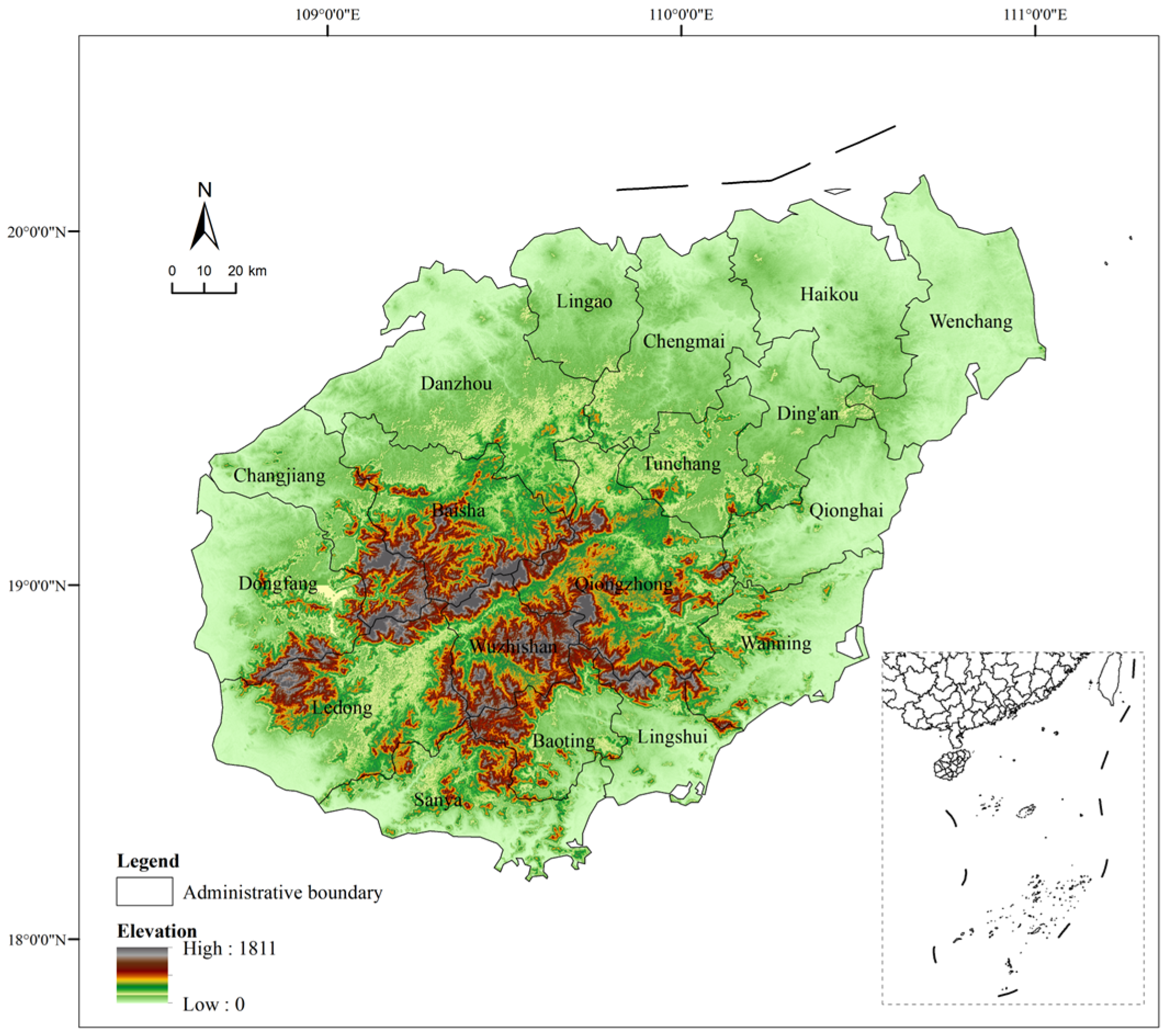
The study area is situated in the northwestern part of the South China Sea and covers the entirety of Hainan Island, China’s largest tropical island, with a land area of approximately 33,900 km2 (Figure 1). The island exhibits a concentric annular topographic pattern, where elevation gradually decreases from the central mountainous interior toward the coastal periphery. Hainan received official approval for International Tourism-Island development in 2009, and tourism has since become its pillar industry. Major tourism hubs such as Sanya and Haikou are distributed across coastal plains and low-elevation terraces, while landscapes with high carbon-sink capacity are concentrated in the central mountainous core. This pronounced spatial gradient between intensive human activity and intact mountain ecosystems provides a natural-experimental setting for investigating human–land coupling mechanisms.
Figure 1.
Location of the study area.
A digital elevation model of Hainan Island showing elevation gradients from the central mountainous interior to the coastal plains. Major cities including Haikou and Sanya are labeled. The map is produced based on the standard map with the approval number GS (2024) 0650, and the administrative boundaries have not been modified.
2.2. Proxy Indicator Selection
Points-of-Interest (POI) data reflect spatial-distribution patterns and agglomeration characteristics of tourism-service facilities. Prior research has used POI datasets to map regional tourism elements [20], and validated their association with the spatial footprint of tourist activities [21]. This study adopts POI kernel density as the proxy for regional tourism-facility intensity (X). Because POI amenities serve both tourists and local residents, kernel-density outputs characterize facility clustering rather than actual tourist visitation volume. We therefore operationalize X as tourism-related facility intensity.
Net primary productivity (NPP) is a core metric for assessing terrestrial-ecosystem carbon-sequestration efficiency [22]. Previous work has applied NPP to evaluate vegetation carbon-sink capacity and its spatiotemporal dynamics [23,24]. This study uses NPP as the proxy for terrestrial tropical-island ecosystem carbon-sink function (Y). NPP quantifies vegetation net primary productivity, measuring the performance of terrestrial vegetation carbon sinks. Throughout this study, the term carbon-sink baseline refers to the spatial distribution and pattern of terrestrial NPP. Conceptually, NPP quantifies vegetation net primary productivity; it does not equate to net ecosystem production (NEP) or total ecosystem carbon sequestration, as it excludes heterotrophic respiration and soil carbon fluxes.
2.3. Data Sources
The datasets used in this study include net primary productivity (NPP), POI-derived kernel density, and land-cover data. All raster datasets correspond to the year 2025, were re-projected to the WGS 1984 UTM Zone 49N projected coordinate system (EPSG:32649), and resampled to a consistent spatial resolution of 487.92 m, yielding a raster grid of 525 columns × 458 rows (458 × 525 cells). The POI vector data were acquired in December 2025, and the MODIS 2025 annual NPP composite was downloaded in April 2026. Detailed data sources and preprocessing workflows are summarized in Table 1.
Table 1.
Data sources and preprocessing.
2.4. Methodology
2.4.1. Pearson Correlation Analysis
Pearson correlation was applied as a descriptive baseline to assess the global linear association between POI kernel density and NPP. As a global, non-directional metric, it quantifies linear co-variation.
2.4.2. Linear Non-Gaussian Acyclic Model (LiNGAM)
We adopted LiNGAM as a linear causal-discovery benchmark to test for detectable linear causal edges between POI kernel density and NPP. The model follows the form:
where x denotes the vector of observed variables, B represents the matrix of causal path coefficients, and e is a vector of independent non-Gaussian error terms [25]. LiNGAM builds upon three assumptions: linear variable relationships, non-Gaussian errors, and no unobserved confounders. Near-zero adjacency coefficients indicate an absence of linear causal links, which motivates the application of the nonlinear GPC model.
2.4.3. Geographical Pattern Causality (GPC) Model
Proposed by Zhang and Wang [19], the Geographical Pattern Causality (GPC) is a pattern-based causal-inference approach built upon the dynamical-systems embedding theory, tailored for static spatial cross-sectional datasets. GPC infers causal direction, classifies outputs into positive, negative, or dark causal subtypes, and quantifies causal strength from spatial-pattern information. It substitutes temporal lags with spatial neighborhood rings: by reconstructing phase-space trajectories from local spatial patterns, GPC evaluates whether the pattern evolution of one variable predicts that of another.
Relationship to existing causal methods. Unlike Granger causality, GPC does not require time-series input, replacing temporal ordering with spatial pixel neighborhood structure. Distinct from CCM/GCCM which test for causal existence and strength, GPC employs symbolic trajectory comparison to differentiate positive, negative, and dark causal subtypes. Subtype labels are sensitive to embedding-parameter settings, which is systematically evaluated in this study (Section 4.2; Appendix A.2).
Spatial embedding and symbolic pattern construction follow the reference GPC workflow [19]. For each valid land pixel, embedding vectors are assembled from the pixel center value plus mean values of successive 8-neighbor rings. Baseline parameters are set as embedding dimension E = 2, lag τ = 1. Here τ represents the spatial-lag step between successive 8-neighborhood rings used for spatial embedding. For each directional test (X→Y, Y→X), embedding trajectories of the predictor variable generate predicted symbol sequences, which are then compared pixel-wise against observed symbol sequences of the response variable. Raw symbol-match counts from the CS matrix are normalized by total valid embedding-comparison positions to yield the overallmatch metric bounded within [0, 1]. Euclidean distance is adopted as the primary metric, with Manhattan and Chebyshev distances included for sensitivity testing. Pixels yielding non-finite embedding vectors are discarded prior to computation. Relative changes along embedding trajectories are converted into symbolic signatures to identify positive, negative, and dark pattern matches. Full mathematical formulation and symbol-encoding rules are provided in Appendix A.
Causal strength and subtype determination. The metric overallmatch quantifies causal-matching strength and is defined as:
where nmatched is the number of pixels with consistent symbolic trajectory matches; and nvalid is the total number of valid pixels available for embedding-based analysis. This metric serves as the primary statistic for comparing bidirectional causal strength (X→Y versus Y→X). GPC evaluates bidirectional predictability: if X→Y markedly exceeds Y→X, it indicates that the spatial pattern of X embeds more information about Y than the reverse. The CS matrix quantifies pattern-match categories; the dominant causal subtype is determined by arg max(CSpositive, CSnegative, CSdark), which reflects the mean matching strength within each category rather than the pixel fraction;. All calculations are executed symmetrically for both directions.
Statistical assessment. Two permutation null models are applied for significance evaluation: valid-internal pixel permutation and block permutation (10 × 10-pixel blocks) that preserves local spatial autocorrelation, with 99 permutations for each test. Block-subsampling with 100 replicates generates 95% confidence intervals for overallmatch, quantifying sampling-driven uncertainty.
Parameter-sensitivity tests are conducted by varying embedding dimension E, lag τ, and distance metrics. We focus on the stability of directional asymmetry calculated as overallmatch (Y→X) − overallmatch (X→Y).
2.4.4. Bivariate Spatial Association (Lee’s L)
Bivariate Lee’s L was implemented within ArcGIS Pro 3.5.4 (Esri, Redlands, CA, USA) to examine local-scale spatial co-clustering between tourism-facility intensity (POI kernel density, X) and terrestrial carbon-sink patterns (NPP, Y). Lee’s L quantifies pairwise spatial-clustering similarity for two variables. Both input rasters (487.92 m, EPSG:32649) were converted to point features and masked to retain only valid land pixels. A K-nearest-neighbor spatial-weight matrix was constructed with K = 8 for each point feature, with automatic row-standardization applied by the software. Local statistical significance was assessed via 999 permutations. For subsequent city-scale statistics, only pixels with statistically significant High–High (HH) clusters (p < 0.05) were used. The city-level HH ratio is defined as the count of significant HH pixels divided by the total number of valid land pixels within each administrative unit.
3. Results
3.1. Island-Wide Scale
Pearson correlation analysis revealed a negligible linear association between POI kernel density and NPP (r = 0.017, p < 0.001, n = 135,419). Although the p-value is significant owing to the large sample size, the effect size is virtually zero, indicating that global linear summaries provide little insight into this relationship. We further applied the Linear Non-Gaussian Acyclic Model (LiNGAM) to test for detectable linear causal edges. Adjacency coefficients were numerically zero for both directions (Table 2). This null outcome confirms the absence of linear causal edges and motivates the application of nonlinear pattern-driven methods.
Table 2.
Comparison of different causal inference methods.
In contrast, the GPC model identified a robust directional asymmetry. overallmatch reached 0.253 for X→Y and 0.486 for Y→X, showing nearly twice the matching strength for the Y→X direction. This asymmetry is supported under both permutation null models: Y→X was statistically significant, whereas X→Y was not statistically significant under either permutation null model (Table 2). Block-subsampling 95% confidence intervals for the two directions do not overlap, confirming the robustness of the directional asymmetry.
Under baseline parameters, the dominant causal subtype is negative for Y→X and positive for X→Y (Table 2). Importantly, the positive-subtype outcome for X→Y represents only a descriptive pattern observed under baseline embedding parameters, rather than a statistically validated causal effect, given the narrow margins between CS-based subtypes and their sensitivity to embedding parameters (Section 4.2). The negative Y→X subtype indicates that areas with strong vegetation carbon-sink patterns exhibit opposing local patterns in tourism-facility density, aligning with intact high-purity carbon-sink cores that exclude dense facility agglomerations. The positive X→Y subtype reflects local co-variation within already developed landscape mosaics. Consequently, our core inference relies on the robust directional asymmetry, treating all subtype labels as parameter-dependent descriptions.
The Y→X > X→Y asymmetry is the core island-wide finding: spatial patterns of vegetation carbon sinks exert a significantly stronger organizing effect on tourism-facility layout than tourism facilities do on carbon-sink configurations. Under baseline parameters, this organizing effect operates negatively at intact carbon-sink cores, manifesting as repelling spatial-pattern correspondence. Rather than supporting oversimplified narratives of tourism destroying ecology or universal mutual co-benefits, this result demonstrates directional spatial coupling. Carbon-sink landscapes act as the dominant spatial organizer for tourism-facility distribution, producing negative pattern correspondence within undisturbed mountain cores and local positive correspondence within human-modified mosaics.
3.2. Subregional-Scale Analysis
While the island-wide GPC analysis indicates a robust Y→X > X→Y directional asymmetry, pixel-wise causality-type composition reveals substantial spatial heterogeneity. To investigate how causal characteristics differ across varying tourism intensities, we classified the 18 cities and counties of Hainan Island into high-density, medium-density, and low-density zones based on the city-level mean of POI kernel density. The zonal statistics (Table 3) show that, island-wide, dark causality accounts for 47.15% of matched pixels, negative causality for 28.28%, and positive causality for 24.57% (X→Y). Dark causality is the largest single category, while positive and negative pixels combined account for slightly more than half of all matched pixels.
Table 3.
Proportions of causality types across zones of different tourism development intensities (X→Y, percentages of matched pixels).
The zonal statistics reveal a weak density gradient in positive proportions, with high- and medium-density zones being nearly indistinguishable. The negative proportion is non-monotonic: highest in the low-density zone, intermediate in the high-density zone, and lowest in the medium-density zone. At the zonal scale, the composition of causality types is only weakly density-dependent, without a clear linear trend.
The Mann–Whitney tests demonstrate that the strength of positive causality differs significantly across zones (p < 0.001 for all pairwise comparisons). Positive-causality pixels in the low-density zone are systematically weaker than those in medium- and high-density zones. Positive strength is similar in magnitude between medium- and high-density zones (0.891 vs. 0.874), though the large pixel-level sample yields a statistically significant difference. This reveals a key distinction between proportion and strength: while facility density does not monotonically increase the share of positive pixels, it modulates the intensity of detected positive interactions.
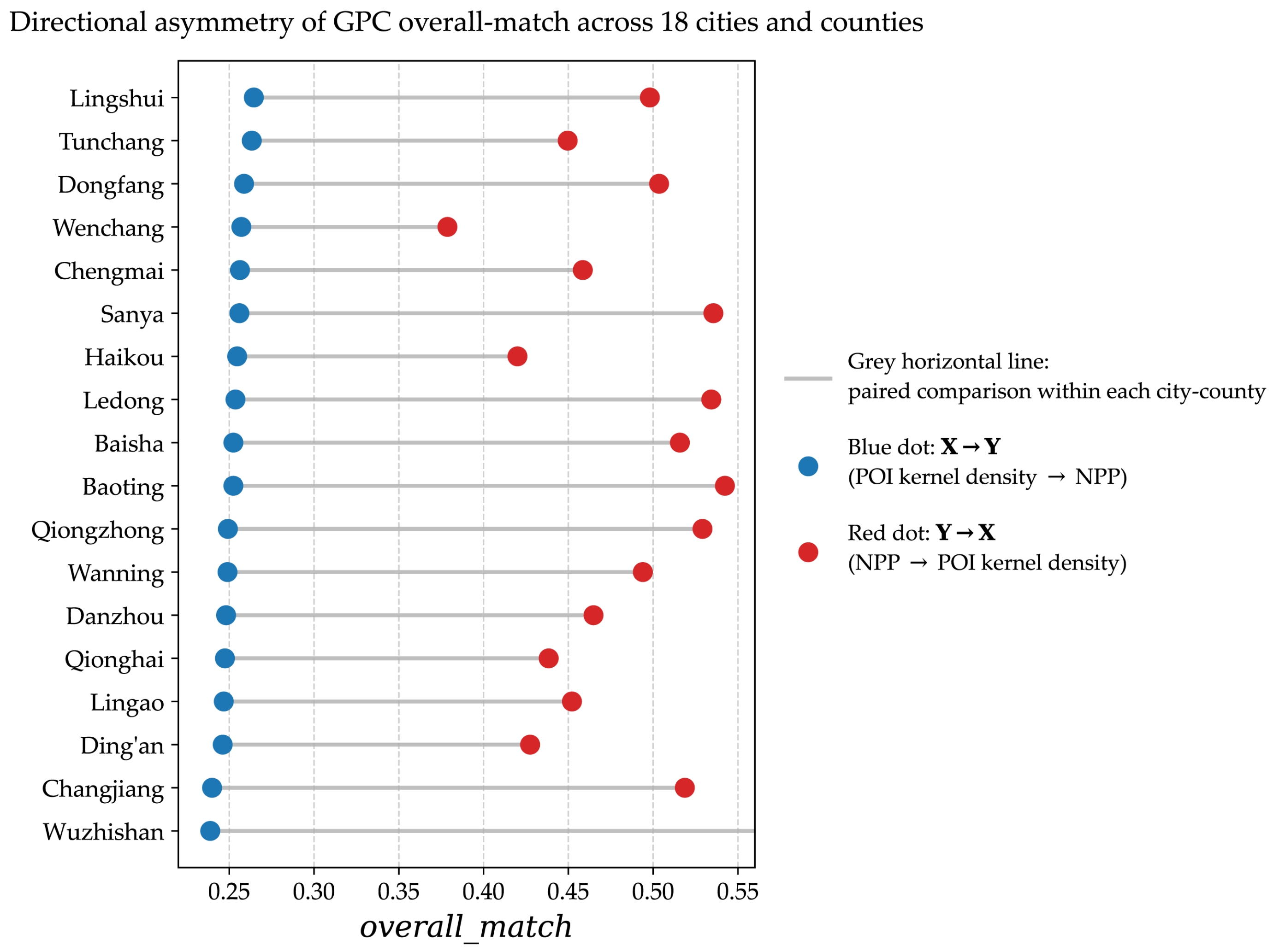
These zonal results support H2 (density–matching interaction). Because positive proportion exhibits weak density dependence whereas positive strength varies substantially across zones, density alone cannot fully structure tourism–NPP coupling. This implicates the spatial co-location of facilities with high-NPP areas as a more plausible explanatory dimension. Because zonal aggregation obscures within-zone heterogeneity, the city-level analysis in Section 3.3 is necessary to isolate this matching mechanism (Figure 2).
Figure 2.
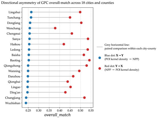
Directional asymmetry of GPC overallmatch across 18 cities and counties. Each row represents a city/county. Blue dots denote the overallmatch for X→Y (POI kernel density to NPP), and red dots denote the overallmatch for Y→X (NPP to POI kernel density). The gray horizontal lines connect the paired comparisons within each city/county. The consistent rightward shift in the red dots relative to the blue dots indicates robust Y→X dominance across the entire island.
3.3. Urban-Scale Comparison
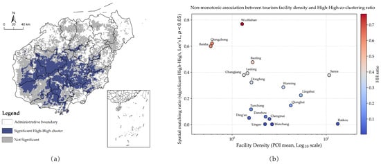
To investigate the differentiation mechanisms at the city scale, we constructed a “density–matching” two-factor classification framework across the 18 cities and counties (Table 4). Facility density was measured by the city-level mean of POI kernel density, while spatial matching (HH ratio) was calculated using Bivariate Spatial Association (Lee’s L), defined strictly as the proportion of pixels with statistically significant High–High clusters (p < 0.05). Splitting both factors into tertiles (33.3% and 66.7% quantiles) organizes the island into seven realized interaction types. The two low-match and two high-match combinations are reported jointly because the density tier does not change their interpretation, yielding five subsections below. No city combines high facility density and high carbon-sink matching. Before interpreting the specific types, a clear conceptual distinction must be made: the significant High–High (HH) co-clustering derived from Lee’s L captures static spatial co-location, whereas the GPC results measure directional symbolic predictability. The two metrics evaluate different spatial properties and should not be conflated (Figure 3).
Table 4.
“Density–match” two-factor classification of each city/county based on GPC results and significant Lee’s L clustering.
Figure 3.
Spatial clustering and non-monotonic density–matching association. (a) Distribution of statistically significant High–High (HH) clusters (dark blue) and not-significant areas (gray) derived from bivariate Lee’s L analysis (p < 0.05), overlaid with city/county administrative boundaries. (The map is based on the standard map with the approval number GS (2024) 0650, with no modifications to the boundaries.) (b) Non-monotonic association between tourism-facility density (mean POI kernel density, log10-scaled x-axis) and the spatial matching ratio (significant HH ratio). Points are colored by their HH ratio on a blue-to-red scale. No smoothing curves or threshold lines are added, preserving the raw observational patterns.
3.3.1. High-Density–Low-Match Type: Spatial Competition in Developed Coasts
This type includes Haikou and Wenchang, characterized by high facility density but HH ratios below 1%. Although GPC captures the robust Y→X > X→Y asymmetry, the descriptive positive GPC matching for X→Y is almost entirely absent, which aligns with the extremely low HH co-clustering observed here. This indicates a clear spatial mismatch between built-up tourism cores and high-NPP regions in highly developed coastal hubs. Intensive tourism infrastructure and high-NPP vegetation rarely co-locate, showing that intense development spatially displaces high-productivity vegetation patches.
3.3.2. High-Density–Medium-Match Type: Localized Fine-Scale Mosaics
This type includes Sanya, Lingshui, Qionghai, and Wanning. Despite high facility density, their HH ratios remain moderate. In Sanya, high-intensity facilities are concentrated within a narrow coastal belt, yet well-preserved riparian and coastal forest belts (e.g., Yalong Bay) remain intact. The presence of moderate HH co-clustering, together with the descriptive positive GPC matching, reflects how localized landscape design and ecological retention sustain spatial synergy with carbon sinks, preventing the complete exclusion observed in Haikou.
3.3.3. Medium-Density and Low-Density–Low-Match Type: Spatial Dispersion
This type includes the medium-density–low-match cities of Chengmai, Danzhou, and Lingao, together with the low-density–low-match city of Ding’an. Facilities and carbon sinks are spatially dispersed, yielding low HH ratios. Without strong spatial matching, neither significant HH co-clustering nor positive GPC matching emerges spatially, while GPC still detects the prevalent Y→X asymmetry.
3.3.4. Medium-Density–Medium-Match Type: The Conventional Transition Zone
This type includes Dongfang and Tunchang, representing a balanced combination where facility density and carbon-sink matching are relatively synchronized. Their HH ratios reflect a typical coupling state under moderate tourism development intensity, where ecological retention balances developmental pressure.
3.3.5. High-Match Type (Medium/Low-Density): Exploratory Hypothesis: Potential Threshold Behavior and Gap Embedding
This type is concentrated in the central mountainous core (e.g., Wuzhishan, Qiongzhong, Baisha, Ledong, Changjiang) and includes Baoting. These counties exhibit the island’s highest HH ratios alongside low facility density.
In Baoting, which has an HH ratio of 0.477, tourism facilities do not form large-scale agglomerations but are embedded within gaps between carbon-sink patches—a spatial configuration consistent with the “gap-embedding” hypothesis. In low-density core areas (e.g., Wuzhishan, Qiongzhong, Baisha), pristine natural forests maintain continuous high carbon-sink density. Here, the carbon-sink pattern acts as a dominant spatial constraint on facility placement. The extremely high HH ratios reflect the pervasive pristine carbon-sink baseline: because nearly the entire landscape matrix is high-NPP, sparse tourism points necessarily co-occur with high carbon sinks. Consistently, the dominant Y→X type in these mountain cores is predominantly dark rather than sharply negative. This configuration is consistent with an ecological threshold at which the carbon-sink pattern shifts from an attractor to a repeller (H3). This observation does not constitute empirical evidence for a transition from attractor to repeller and requires further independent validation.
4. Discussion
4.1. Beyond the Trade-Off Narrative: Asymmetric Spatial Coupling
Recent methodological advances in spatial causal inference emphasize directional asymmetry rather than merely detecting statistical association [26]. The GPC approach adopted here extends this by working with static spatial cross-sections and distinguishing positive, negative, and dark causal subtypes. This study reveals a complex human–land coupling logic between tourism-facility intensity and terrestrial vegetation carbon-sink patterns.
In contrast to the near-zero linear correlation and negligible LiNGAM coefficients, the GPC model identifies robust directional asymmetry, with overallmatch for Y→X substantially exceeding X→Y. Global linear summaries yield little insight into this dataset. The two methods differ fundamentally in their analytical targets—global linear co-variation versus local symbolic predictability within reconstructed phase space—and their results are complementary [17].
Consistent with prior work framing tourism as an important carbon source [27,28], this study adds a causal-directional perspective. At the landscape scale, high-standard tourism facilities such as luxury hotels and golf courses co-occur with retained green carbon-sink vegetation within developed mosaics [29], consistent with the positive X→Y type. More importantly, the Y→X > X→Y asymmetry reframes island tourism theory: high-NPP landscapes are not merely passive background constraints, but spatial organizers that guide the placement of tourism facilities. This carbon-sink-pattern-first interpretation resonates with regenerative tourism scholarship [30,31]. The negative Y→X signature indicates spatial repulsion within intact high-purity cores. Positive X→Y coupling within developed mosaics reflects local co-variation between vegetation productivity and facility density, which coexists with aggregate carbon costs from tourism construction and transport. This coast-interior polarization aligns with recent national-scale evidence on tourism carbon efficiency, showing high-efficiency clusters in coastal regions while interior destinations face geographical constraints [32].
4.2. Density, Parameter Sensitivity, and the Limits of Type Interpretation
Zonal results show that the strength of positive causality varies significantly across POI-density zones, while the proportion of positive pixels changes only weakly. Tourism density is therefore not a linear driver of positive-pixel shares. City-scale Lee’s L analysis further highlights pronounced polarization in statistically significant High–High (HH) clustering. High-density coastal cities show near-zero HH ratios, meaning intensive tourism agglomerations rarely co-locate with high-NPP vegetation. By contrast, low-density mountainous counties in the central core exhibit the highest HH ratios. This polarization corroborates the GPC-derived Y→X asymmetry: carbon-sink patterns constitute the dominant spatial constraint on facility placement. Near-zero HH values in coastal urban zones reflect spatial mismatch between tourism infrastructure and carbon-sink hotspots. High HH ratios in undisturbed mountain cores are largely driven by the widespread high-NPP background matrix: sparse tourism sites inevitably overlap with high-productivity areas. This coast-interior spatial polarization aligns with land-use carbon-emission patterns documented for Hainan Island, where emission growth concentrates in coastal zones and the mountainous interior maintains low-emission conditions [33].
Parameter-sensitivity tests show that directional asymmetry remains robust across all tested parameter combinations, whereas dominant causal types are parameter-dependent. We therefore anchor our core inference on the bidirectional strength asymmetry and treat subtype labels as descriptive outputs.
For the threshold hypothesis (H3) and gap-embedding mechanism, Lee’s L clustering provides descriptive spatial evidence [34]. For Baoting, the significant HH ratio of 0.477 shows tourism facilities embedded within gaps between carbon-sink patches, before exclusion effects emerge in the highest-purity cores. Due to the limited sample of 18 cities, formal threshold estimation is not supported; H3 remains a working conjecture.
4.3. From Hainan to Global Tropical Islands: Governance Implications and Transferability
The spatial causal atlas produced here supports place-specific governance for tropical islands. Instead of uniform tourism density caps or blanket conservation rules, management should acknowledge that carbon-sink patterns structure tourism distribution more strongly than tourism shapes carbon sinks, with repelling effects in intact cores and local positive co-variation within developed mosaics. This implies a governance strategy that protects continuous high-NPP cores as spatial organizers while concentrating new tourism development within ecologically matched mosaics instead of expanding into natural frontiers. This logic resonates with emerging carbon-neutrality frameworks for tourism-dependent regions, which note that construction-land encroachment can erode land-use carbon sinks even alongside local urban greening measures [35]. For Hainan, the spatial placement of tourism development relative to intact high-NPP cores carries comparable importance to aggregate development intensity. This approach aligns with place-based island tourism governance [1,36] and context-sensitive sustainability frameworks [37].
The Hainan case yields transferable insights for other tropical islands. The directional-asymmetry workflow serves as a diagnostic tool to evaluate whether carbon-sink patterns or tourism density act as the stronger spatial organizer in a given destination. Moreover, the distinction between the proportion and strength of positive causality warns against relying solely on pixel fractions as management indicators. The parameter dependence of causal types also cautions against designing rigid policies based on a single static subtype classification. These insights are especially relevant for small island developing states, where tourism dependence, ecological vulnerability, and fiscal constraints create severe sustainability trade-offs [38,39]. The asymmetry test is transferable as an analytical template, but its application elsewhere requires local calibration of parameters, proxies, and spatial scales.
4.4. Limitations and Future Work
This study is bounded by its methodological and data constraints. Based on a 2025 static spatial snapshot, GPC identifies spatial-pattern associations rather than temporally ordered causal processes; temporal or quasi-experimental designs are required to capture dynamic causality. Additionally, dominant causal subtypes vary with embedding dimension and lag settings, so our core inference relies on the robust directional asymmetry, treating subtype labels as parameter-dependent descriptions. Although permutation and subsampling tests address randomization and sampling uncertainty, GPC cannot fully exclude unobserved shared drivers such as topography, climate, or conservation status. Furthermore, the proxy data carry inherent limits: POI records include facilities serving local residents, and NPP does not capture soil, coastal, or marine carbon sinks.
Future work should extend GPC to spatiotemporal datasets to trace dynamic processes. Incorporating quasi-experimental or structural causal designs would help adjust for unobserved confounding. Testing threshold and gap-embedding hypotheses with larger samples will clarify their mechanisms, and applying this combined GPC–Lee’s L framework to other tropical islands will enable comparative analysis.
5. Conclusions
In this study, we applied the Geographical Pattern Causality (GPC) model to 2025 POI kernel density and NPP data on Hainan Island to unveil the spatial causal structure between tourism development and vegetation carbon-sink patterns in a tropical island setting.
Conventional linear methods detect no meaningful association between tourism-facility density and vegetation carbon sinks. In contrast, GPC reveals a robust directional asymmetry: the spatial pattern of vegetation carbon sinks exerts a significantly stronger organizing effect on tourism-facility layout than tourism-facility density does on the carbon-sink pattern. At baseline parameters, this organizing effect manifests as a negative causal type for Y→X, consistent with high-purity carbon-sink cores excluding facility concentration, and a positive type for X→Y, reflecting local co-variation within already developed tourism mosaics.
This directional asymmetry is highly robust, remaining consistent across all tested parameter combinations and reproduced across all 18 cities and counties. The integration of Lee’s L further reveals a marked spatial polarization: significant High–High co-location is nearly absent in high-density coastal tourism hubs but dominates in low-density pristine carbon-sink cores. Alongside the localized gap-embedding pattern observed in medium-density areas such as Baoting, this spatial evidence supports a vegetation-carbon-sink-pattern-first logic.
These findings reframe the tourism–carbon-sink relationship in tropical islands from a simple trade-off to an asymmetric spatial coupling. For governance, this implies that the one-place-one-policy should not rely on uniform density caps or blanket conservation rules. Instead, continuous high-NPP cores should be recognized as spatial organizers that constrain facility placement, while tourism development is concentrated in already developed mosaics rather than frontier expansion. Local positive coupling within developed mosaics reflects co-variation in facility density and retained NPP, though it does not guarantee overall climate benefits given the aggregate carbon costs of tourism transport and construction.
Future research should test the observed spatial-pattern asymmetry using time-series or quasi-experimental designs. Extending the combined GPC–Lee’s L framework to other tropical island destinations, with locally calibrated parameters and proxies, will enable robust comparative research on tourism–ecology coupling.
Author Contributions
Conceptualization, F.W.; methodology, D.L.; software, D.L.; validation, F.W.; formal analysis, D.L.; investigation, D.L.; data curation, D.L.; writing—original draft preparation, D.L.; writing—review and editing, F.W.; visualization, D.L.; supervision, F.W.; project administration, F.W. All authors have read and agreed to the published version of the manuscript.
Funding
This research was funded by the National Key Research and Development Program of China, grant number 2022YFD2401301; and the Philosophy and Social Science Research Base Project of Hainan Province, grant number HNSK(JD)24-07.
Data Availability Statement
The data and code supporting the findings of this study are openly available on Figshare at https://doi.org/10.6084/m9.figshare.33261714. The dataset includes the net primary productivity (NPP) raster, POI kernel density raster, land-cover data, zone classification raster, and shapefiles for 18 cities and counties of Hainan Island. The Python 3.12.6 (Python Software Foundation, Wilmington, DE, USA) code reproduces the GPC workflow, including data preprocessing, global and zonal GPC analysis, baseline comparisons, robustness tests, and city-level causal statistics. The code was developed using PyCharm 2024.2.4 (JetBrains, Prague, Czech Republic). The bivariate Lee’s L analysis was performed in ArcGIS Pro 3.5.4 (Esri, Redlands, CA, USA); the exported point file (Points_Final.shp) and calc_hh_ratio.py are provided to reproduce the city-level HH ratios used in Table 4. Table 4_Final.csv and city_causal_stat.csv are included to reproduce Figure 2 and Figure 3 and Table 4.
Acknowledgments
The authors are grateful for the valuable suggestions from the editor and the anonymous reviewers. During the preparation of this manuscript, the authors used DeepSeek V3 for the purposes of improving the readability and language of the manuscript. The authors have reviewed and edited the output and take full responsibility for the content of this publication.
Conflicts of Interest
The authors declare no conflicts of interest. The funders had no role in the design of the study; in the collection, analyses, or interpretation of data; in the writing of the manuscript; or in the decision to publish the results.
Appendix A. Supplementary Implementation Details of the GPC Model
Appendix A.1. Spatial Embedding and Symbolic Encoding
Rationale for reading overallmatch as a directional strength indicator. According to Takens’ theorem [40] and the generalized embedding principle [41], in deterministic or weakly coupled systems, if variable X directionally influences variable Y, X’s delay-coordinate reconstructed manifold can retain information about the states of Y; accordingly, cross-mapping from X’s reconstructed states to Y can serve as an operational indicator of directional pattern-based coupling [42]. In our cross-sectional GPC framework, a higher overallmatch (X→Y) indicates that the reconstructed spatial states of X provide more reliable cross-predictive consistency for the symbol sequence of Y. This predictive consistency is an operational indicator of directional associational coupling and does not constitute definitive proof of physical causal mechanisms. Evidence for causality comes only from statistically significant directional asymmetry in predictive performance relative to appropriate null models/surrogates, together with convergence checks; the interpretation remains subject to unobserved spatial confounders as noted in Section 4.4.
For each valid land pixel i, GPC constructs an embedding vector from the focal-pixel value and mean values of successive surrounding 8-neighbor rings:
In this formulation, V(i) represents the spatial-embedding vector for pixel (i)z(i) and is the observed value of the target variable (either POI kernel density or NPP) at the focal pixel i. (i,k) denotes the mean value of the k-th-order 8-neighborhood ring surrounding pixel i, where k∈[1, E]. E denotes the embedding dimension, so the embedding vector thus contains E + 1 components (focal-pixel value plus E ring-averaged values). The parameter τ defines the spatial step between successive neighborhood rings for spatial embedding; under our baseline setting E = 2, τ = 1, the total number of neighborhood rings used for embedding is given by lag = 2E + 1 = 5.
Trajectories formed by successive vector components are transformed into three symbolic states: ↑ = 3 (increase), → = 2 (no change), and ↓ = 1 (decrease). Symbol-sequence comparison is performed pixel-wise between the two variables. No variable standardization is applied prior to embedding; the symbolization compares relative changes within each embedding trajectory and is therefore scale-free.
Positive match: Predicted and observed symbol sequences are element-wise identical.
Negative match: Predicted and observed symbol sequences are element-wise opposite (1 ↔ 3).
Dark match: Neither identical nor opposite patterns (including fully neutral sequences).
The CS matrix stores pixel counts for these three categories. CSmax is used solely to label the dominant subtype and is not a formal statistical test statistic.
Step-by-Step GPC Workflow
- (1)
- Construct spatial-embedding vectors for predictor and response variables from focal-pixel values plus mean values of successive 8-neighbor rings, controlled by embedding dimension E and spatial lag τ.
- (2)
- Convert each embedding trajectory into three symbolic states: increase, no change, decrease.
- (3)
- For each causal direction, generate predicted symbol sequences from the predictor embedding trajectory.
- (4)
- Compare predicted and observed symbol sequences pixel-by-pixel and classify each comparison as positive match, negative match, or dark match.
- (5)
- Aggregate match counts and normalize to compute the overallmatch statistic.
- (6)
- Conduct valid-internal and block-permutation significance assessment for directional pattern-matching strength.
Appendix A.2. Full Parameter-Sensitivity Results
Table A1 reports complete one-at-a-time sensitivity results supporting Section 4.2. The baseline setting is E = 2, τ = 1, Euclidean distance; spatial lag length equals 5 under baseline and increases to 7, 9, and 11 for E = 3, E = 4, and E = 5, respectively.
Table A1.
Parameter sensitivity of GPC outputs across embedding dimension (E), lag order (τ), and distance metric.
Appendix A.3. Pixel Filtering and Matched-Pixel Accounting
The analysis grid has dimensions 458 × 525, yielding 135,419 valid land pixels (56.32% of total grid cells). Pixels producing non-finite embedding vectors originating from raster boundaries and coastal masking are discarded prior to pattern matching. This filtering yields 135,103 valid pixels for E = 2; 135,099 for E = 3; 135,098 for E = 4 and E = 5. Under baseline parameters, matched-pixel counts are 34,134 for X→Y and 65,648 for Y→X, consistent with overallmatc values presented in Section 3.1.
To ensure all reported metrics remain bounded within [0, 1], the per-pixel CS matching-strength values are normalized using the Gaussian error function (erf) prior to determining the dominant subtype. In contrast, overallmatc is defined as a simple count ratio and is intrinsically bounded within [0, 1] without any transformation.
Explicit accounting of valid and matched pixels. For a directional test, nvalid is the number of pixels whose embedding vector is fully finite:
where N is the total number of grid cells and I(·) is the indicator function. nmatched counts the pixels that receive a classifiable comparison in that direction:
At baseline parameters nvalid = 135,103, and nmatched = 34,134 for X→Y and 65,648 for Y→X, yielding overallmat values of 0.253 and 0.486, respectively. Consequently, CSmax reports the mean matching strength for each causal class, whereas the pixel-level subtype fractions reported in Table 3 are calculated specifically over the nmatched population.
References
- McLeod, M. Island tourism: Past, present, and prospects. Tour. Geogr. 2025, 27, 798–809. [Google Scholar] [CrossRef] [Scilit]
- Hamzah, A.; Hampton, M.P. Resilience and non-linear change in island tourism. Tour. Geogr. 2013, 15, 43–67. [Google Scholar] [CrossRef] [Scilit]
- Pi, Z.; Liu, X.; Wei, Y.; Wang, X.; Zang, Z.; Song, X. Spatiotemporal variation in carbon sequestration in the forest ecosystem of Hainan Island over a 30-year period and its driving factors. Ecol. Indic. 2026, 182, 114587. [Google Scholar] [CrossRef] [Scilit]
- Liu, Q.; Yang, D.; Cao, L.; Anderson, B. Assessment and prediction of carbon storage based on land use/land cover dynamics in the tropics: A case study of Hainan Island, China. Land 2022, 11, 244. [Google Scholar] [CrossRef] [Scilit]
- He, D.; Chen, K.; Zhang, T.; Yin, M.; Shi, X.; Xu, Z. Regional CO2 budget and abatement countermeasures for forest scenic spots: A case study of the Shenyang National Forest Park. Sustainability 2021, 13, 861. [Google Scholar] [CrossRef] [Scilit]
- Yang, M.; Lu, P.; Tsai, C.-H.; Huang, X.; Chen, X.; Chen, D. Spatiotemporal coupling and coordination of tourism and the production-living-ecological system in Hainan Island, China. Discov. Sustain. 2026, 7, 1050. [Google Scholar] [CrossRef] [Scilit]
- Lenzen, M.; Sun, Y.-Y.; Faturay, F.; Ting, Y.-P.; Geschke, A.; Malik, A. The carbon footprint of global tourism. Nat. Clim. Change 2018, 8, 522–528, Correction in Nat. Clim. Change 2018, 8, 544. [Google Scholar] [CrossRef] [Scilit]
- WTTC (World Travel & Tourism Council). Travel & Tourism Economic Impact 2023. Available online: https://wttc.org/research/economic-impact (accessed on 15 October 2026).
- Feng, D.; Li, C.; Li, Y. Study on spatial-temporal evolution, decoupling effect and influencing factors of tourism transportation carbon emissions: Taking North China as an example. Atmosphere 2024, 15, 720. [Google Scholar] [CrossRef] [Scilit]
- Pan, Z.; Luo, Y.; Wang, Y.; Ji, J.; Lai, B. Coupling coordination and driving mechanism between tourism development, ecological conservation and digital economy: Insights from Chinese 278 cities. Sci. Rep. 2025, 15, 37445. [Google Scholar] [CrossRef] [Scilit] [PubMed]
- Liu, T.; Zhao, S.; Peng, F. Tourism-driven commodification of island landscapes: An actor-network analysis of dynamic mechanisms in Guanglu Island, China. Chin. Geogr. Sci. 2025, 35, 867–881. [Google Scholar] [CrossRef] [Scilit]
- Zhu, L.; Zhou, Y. Coupling of island tourism carbon emission and sustainable resource development-taking Hainan Fenjie Island as an example. Int. J. Sustain. Energy 2023, 42, 1391–1406. [Google Scholar] [CrossRef] [Scilit]
- Becken, S. Developing a framework for assessing resilience of tourism sub-systems to climatic factors. Ann. Tour. Res. 2013, 43, 506–528. [Google Scholar] [CrossRef] [Scilit]
- Strickland-Munro, J.K.; Allison, H.E.; Moore, S.A. Using resilience concepts to investigate the impacts of protected area tourism on communities. Ann. Tour. Res. 2010, 37, 499–519. [Google Scholar] [CrossRef] [Scilit]
- Folke, C.; Carpenter, S.R.; Walker, B.; Scheffer, M.; Chapin, F.S., III; Rockström, J. Resilience thinking: Integrating resilience, adaptability and transformability. Ecol. Soc. 2010, 15, 20. [Google Scholar] [CrossRef] [Scilit]
- Gao, B.; Wang, J.; Stein, A.; Chen, Z. Causal inference in spatial statistics. Spat. Stat. 2022, 50, 100621. [Google Scholar] [CrossRef] [Scilit]
- Gao, B.; Yang, J.; Chen, Z.; Sugihara, G.; Li, M.; Stein, A.; Kwan, M.P.; Wang, J. Causal inference from cross-sectional earth system data with geographical convergent cross mapping. Nat. Commun. 2023, 14, 5875, Correction in Nat. Commun. 2023, 14, 7288. [Google Scholar] [CrossRef] [Scilit] [PubMed]
- Lebel, L.; Anderies, J.M.; Campbell, B.; Folke, C.; Hatfield-Dodds, S.; Hughes, T.P.; Wilson, J. Governance and the capacity to manage resilience in regional social-ecological systems. Ecol. Soc. 2006, 11, 19. [Google Scholar] [CrossRef] [Scilit]
- Zhang, Z.; Wang, J. A model to identify causality for geographic patterns. Int. J. Geogr. Inf. Sci. 2026, 40, 1972–1992. [Google Scholar] [CrossRef] [Scilit]
- Jiang, Y.; Huang, W.; Xiong, X.; Shu, B.; Yang, J.; Li, M.; Cui, X. Investigating spatial patterns and determinants of tourist attractions utilizing POI data: A case study of Hubei Province, China. Heliyon 2024, 10, e32370. [Google Scholar] [CrossRef] [Scilit] [PubMed]
- Barrena-Herrán, M.; Modrego-Monforte, I.; Grijalba, O. Mapping the spatiotemporal urban footprint of residents and tourists: A data-driven approach based on user-generated reviews. ISPRS Int. J. Geo-Inf. 2025, 14, 456. [Google Scholar] [CrossRef] [Scilit]
- Wu, L.; Zhang, Y.; Luo, G.; Chen, D.; Yang, D.; Yang, Y.; Tian, F. Characteristics of vegetation carbon sink carrying capacity and restoration potential of China in recent 40 years. Front. For. Glob. Change 2023, 6, 1266688. [Google Scholar] [CrossRef] [Scilit]
- Song, L.; Li, M.; Xu, H.; Guo, Y.; Wang, Z.; Li, Y.; Wu, X.; Feng, L.; Chen, J.; Lu, X.; et al. Spatiotemporal variation and driving factors of vegetation net primary productivity in a typical karst area in China from 2000 to 2010. Ecol. Indic. 2021, 132, 108280. [Google Scholar] [CrossRef] [Scilit]
- Wang, T.; Gao, M.; Fu, Q.; Chen, J. Spatiotemporal dynamics and influencing factors of vegetation net primary productivity in the Yangtze River Delta Region, China. Land 2024, 13, 440. [Google Scholar] [CrossRef] [Scilit]
- Shimizu, S.; Hoyer, P.O.; Hyvärinen, A.; Kerminen, A. A linear non-Gaussian acyclic model for causal discovery. J. Mach. Learn. Res. 2006, 7, 2003–2030. Available online: https://jmlr.org/papers/v7/shimizu06a.html.
- Zhang, Y.; Hong, Y.; Gao, S.; Raubal, M. Bidirectional yet Asymmetric Causality between Urban Systems and Traffic Dynamics in 30 Cities Worldwide. Nat. Commun. 2026, 17, 4671. [Google Scholar] [CrossRef] [Scilit] [PubMed]
- Gössling, S.; Balas, M.; Mayer, M.; Sun, Y.-Y. A review of tourism and climate change mitigation: The scales, scopes, stakeholders and strategies of carbon management. Tour. Manag. 2023, 95, 104681. [Google Scholar] [CrossRef] [Scilit]
- Scott, D.; Hall, C.M.; Rushton, B.; Gössling, S. A review of the IPCC sixth assessment and implications for tourism development and sectoral climate action. J. Sustain. Tour. 2024, 32, 1725–1742. [Google Scholar] [CrossRef] [Scilit]
- Wang, L.; Zhao, H.; Wu, W.; Song, W.; Zhou, Q.; Ye, Y. Time-varying evolution and impact analysis of forest tourism carbon emissions and forest park carbon sinks in China. Forests 2024, 15, 1517. [Google Scholar] [CrossRef] [Scilit]
- Bellato, L.; Frantzeskaki, N.; Nygaard, C.A. Regenerative tourism: A conceptual framework leveraging theory and practice. Tour. Geogr. 2023, 25, 1026–1046. [Google Scholar] [CrossRef] [Scilit]
- Becken, S.; Kaur, J. Anchoring “tourism value” within a regenerative tourism paradigm-a government perspective. J. Sustain. Tour. 2022, 30, 52–68. [Google Scholar] [CrossRef] [Scilit]
- Wang, R.; Hao, J.-X.; Wang, C.; Yu, Y. Aviation Big Data-Driven Tourism Carbon Efficiency Evaluation: Evidence from China. J. Sustain. Tour. 2026, 34, 213–241. [Google Scholar] [CrossRef] [Scilit]
- Mao, M.; Ma, Y.; Yang, Y.; Jia, J.; Gong, W.; Wu, L. Spatiotemporal Evolution and Associated Factors of Land Use Carbon Emissions on Hainan Island, China. Land 2026, 15, 1490. [Google Scholar] [CrossRef] [Scilit]
- Perng, L.Y.; Leong, K.M.; Weijerman, M.; Oleson, K.L.L. A multi-decadal assessment of social thresholds and outcomes in marine social-ecological systems in Hawaiʻi. Mar. Policy 2024, 163, 106141. [Google Scholar] [CrossRef] [Scilit]
- Li, H.; Tong, Y. Developing a Quantitative Analytical Framework for Carbon Neutrality in Tourism-Dependent Regions. Humanit. Soc. Sci. Commun. 2025, 12, 797–818. [Google Scholar] [CrossRef] [Scilit]
- Hung, Y.-T.; Tsou, C. From carrying capacity to destination resilience: An indicator framework for island tourism. Tour. Geogr. 2026, 28, 141–162. [Google Scholar] [CrossRef] [Scilit]
- Wang, T.; Yang, Z.; Ma, X.; Han, F.; Zheng, X. Resilience of tourism social-ecological systems: Conceptualization and research framework. Environ. Dev. Sustain. 2025, 1–25. [Google Scholar] [CrossRef] [Scilit]
- Allen, M. Climate-resilient actor-networks for island tourism. Tour. Geogr. 2026, 28, 773–794. [Google Scholar] [CrossRef] [Scilit]
- Santana-Padrón, A.; Lam-González, Y.E.; De León, J. Tourist heterogeneity in carbon compensation: A two-stage framework for sustainable island tourism policy. Ann. Tour. Res. Empir. Insights 2026, 7, 100222. [Google Scholar] [CrossRef] [Scilit]
- Takens, F. Detecting strange attractors in turbulence. In Dynamical Systems and Turbulence; Rand, D., Young, L.-S., Eds.; Springer: Berlin/Heidelberg, Germany, 1981; pp. 366–381. [Google Scholar] [CrossRef] [Scilit]
- Sauer, T.; Yorke, J.A.; Casdagli, M. Embedology. J. Stat. Phys. 1991, 65, 579–616. [Google Scholar] [CrossRef] [Scilit]
- Sugihara, G.; May, R.; Ye, H.; Hsieh, C.H.; Deyle, E.; Fogarty, M.; Munch, S. Detecting causality in complex ecosystems. Science 2012, 338, 496–500. [Google Scholar] [CrossRef] [Scilit] [PubMed]

Disclaimer/Publisher’s Note: The statements, opinions and data contained in all publications are solely those of the individual author(s) and contributor(s) and not of MDPI and/or the editor(s). MDPI and/or the editor(s) disclaim responsibility for any injury to people or property resulting from any ideas, methods, instructions or products referred to in the content. |
© 2026 by the authors. Licensee MDPI, Basel, Switzerland. This article is an open access article distributed under the terms and conditions of the Creative Commons Attribution (CC BY) license.