


Highlights
What are the main findings?
- •
- High or very high agricultural potential covered 46.7% of the basin, mainly in the Lower Paraopeba.
- •
- Land-use capability drove the pattern; priority areas kept their class in 92% of Monte Carlo runs.
What are the implications of the main findings?
- •
- About 3000 km2 of high-potential pastures can be intensified without clearing native vegetation.
- •
- The open-data GIS–AHP framework can support regional agricultural planning in other basins.
Abstract
Growing demand for food requires expanding and intensifying agriculture while maintaining environmental and economic sustainability. This study mapped agricultural potential—the relative, crop-independent capacity of land to support rainfed agricultural use (crops, pastures, and planted forests)—in the Paraopeba River Basin, Brazil, using GIS-based multicriteria decision analysis. Land-use capability, simplified climatic water balance, agricultural production value per hectare, and distance to roads were rescaled with linear fuzzy functions and combined by a weighted linear combination using Analytic Hierarchy Process weights (56.5%, 26.2%, 11.8%, and 5.5%, respectively; consistency ratio = 4.3%). Low (26.4%) and high (27.2%) potential predominated. High-potential areas were concentrated in the Lower Paraopeba and on the left bank, whereas low-potential areas predominated in the Upper Paraopeba and on the right bank, mainly driven by land-use capability. In a Monte Carlo analysis of the AHP judgments, priority areas retained their class in 92% of simulations. Because land use was used to build the economic criterion, the agreement with current agriculture is descriptive rather than an independent validation; a scenario without this criterion discriminated agricultural land from natural vegetation with an area under the curve of 0.63. The framework supports regional planning, but high potential does not justify converting native vegetation.
1. Introduction
With the constant increase in global population, new areas must be incorporated into agricultural production systems to meet the worldwide demand for food [1]. However, the expansion of the agricultural frontier has been hindered by environmental and socioeconomic constraints, as well as conflicts among different land-use types.
Thus, identifying and allocating areas with higher agricultural potential—considering agronomic, environmental, and socioeconomic aspects—are essential for the sustainable and efficient development of agriculture, and consequently for minimizing negative environmental impacts, promoting soil conservation, and ensuring the economic and environmental viability of rural properties [1,2,3].
Moreover, identifying areas with greater agricultural potential provides significant benefits such as increased productivity, reduced production costs, and the mitigation of environmental risks [2]. It also enables more precise planning and implementation of sustainable agricultural practices, thereby contributing to the socioeconomic development of rural regions [4].
Rational land use allows agricultural production to be optimized and the economic performance of farming activities to be improved. However, achieving rational land use requires knowledge of land-use capability, ensuring that the intensity of cultivation does not reduce its productive capacity in the medium and long term [2,4,5]. Therefore, when selecting an area for agricultural exploitation, it is essential to consider its pedological, topographic, and local climatic characteristics [6].
According to Lepsch et al. [7], land-use capability is the first step in soil conservation and is a crucial tool for rational land use, as it enables the identification of soil aptitudes and limitations for different types of crops. Using land according to its capability maximizes productivity and makes production systems efficient, rational, and intensive without causing degradation [6,8].
Integrating land occupation—which involves analyzing current agricultural practices and land-use patterns—with economic performance assessments provides a holistic perspective that supports more assertive decision-making regarding the selection of new agricultural areas and the management of already productive lands [3,9].
Several studies have sought to identify areas with greater agricultural potential [1,2,3,4,10,11]. However, some of these investigations considered only soil and terrain characteristics or field-based data, which are not always available in other regions. Taveira et al. [12] note that despite the importance of including socioeconomic factors in land-use capability assessments, few studies have done so. Özkan et al. [1] further suggest that incorporating socioeconomic data is essential for evaluating agricultural potential and should be the next step in land-use planning.
Existing GIS–MCDA studies of agricultural land suitability have three main limitations. First, most are crop-specific and depend on detailed soil, climate, and field data that are not available for many regions [1,2,3,11,13]. Second, they usually consider only biophysical criteria, whereas socioeconomic variables, such as economic performance and accessibility, are seldom included [12]. Third, the AHP weights are generally treated as fixed, and their influence on the results is rarely tested [14,15]. In Brazil, the land-use capability system is widely applied at the farm and watershed scales [5,16,17], but it has rarely been combined with climatic water availability, economic performance, and accessibility in a single basin-scale index. The novelty of the present study therefore lies in (i) using the Brazilian land-use capability system, derived from open soil and terrain data, as the agronomic core of a crop-independent agricultural potential index; (ii) coupling it with a remotely sensed climatic water balance and with municipal economic and accessibility indicators; and (iii) explicitly evaluating the sensitivity of the resulting classification to the AHP weights. Because the framework relies exclusively on open-access datasets, it can be replicated in other basins where detailed field data are not available.
In this context, this study aims to develop and apply a methodology that integrates land-use capability, climatic water balance, economic performance, and accessibility to identify priority areas for agricultural development in the Paraopeba River Basin, Brazil, and to evaluate the robustness of the results to the criterion weights. Here, agricultural potential is defined as the relative capacity of an area to support agricultural use in general—crops, pastures, and planted forests, rather than a specific crop—under rainfed conditions. It is a composite index that combines biophysical suitability (land-use capability and climatic water balance, which together account for 82.7% of the weights), the regional economic context of agriculture (11.8%), and accessibility (5.5%); it therefore expresses mainly biophysical suitability, adjusted by economic and accessibility conditions. It expresses relative suitability within the basin and not the legal or environmental feasibility of converting land to agriculture. The application of this methodology seeks to support public policies and strategies for agricultural expansion, promoting sustainability and efficiency in the use of natural resources.
The specific objectives were to (i) map agricultural potential in the Paraopeba River Basin by integrating land-use capability, climatic water balance, agricultural production value per hectare, and distance to roads through AHP and WLC (Section 2.2, Section 2.3, Section 3.1, Section 3.2 and Section 3.3); (ii) identify the criteria that drive the spatial pattern of agricultural potential (Section 3.2, Section 3.3 and Section 4.1); (iii) assess the robustness of the classification to the AHP weights (Section 2.4 and Section 3.4); and (iv) compare the results with current land use and discuss the limitations and planning implications of the framework, including the distinction between agricultural potential and the feasibility of agricultural expansion (Section 3.5, Section 4.2, Section 4.3, Section 4.4 and Section 4.5).
2. Materials and Methods
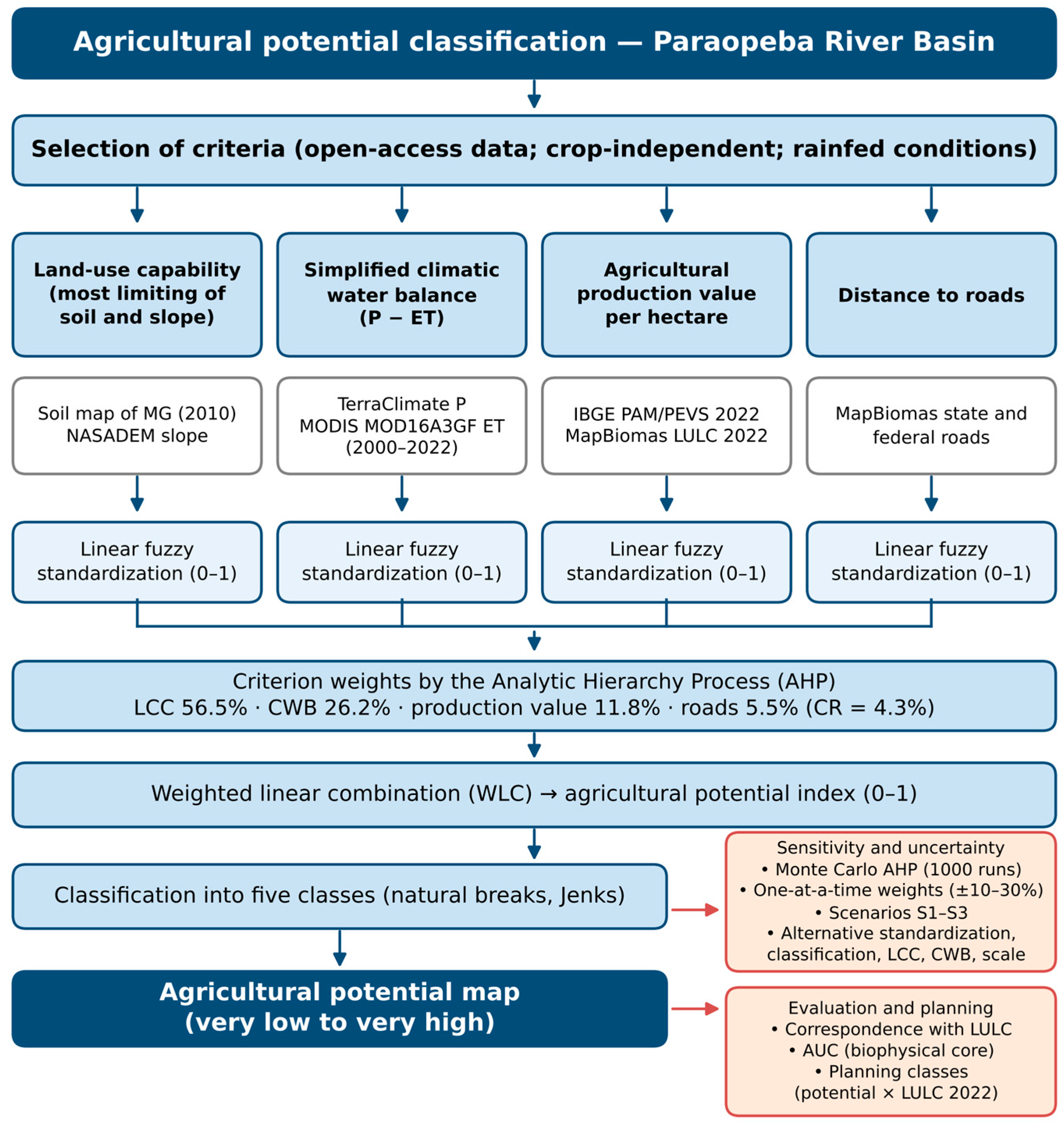
The process for classifying the agricultural potential of the Paraopeba River Basin was carried out according to the flowchart presented in Figure 1.
2.1. Study Area
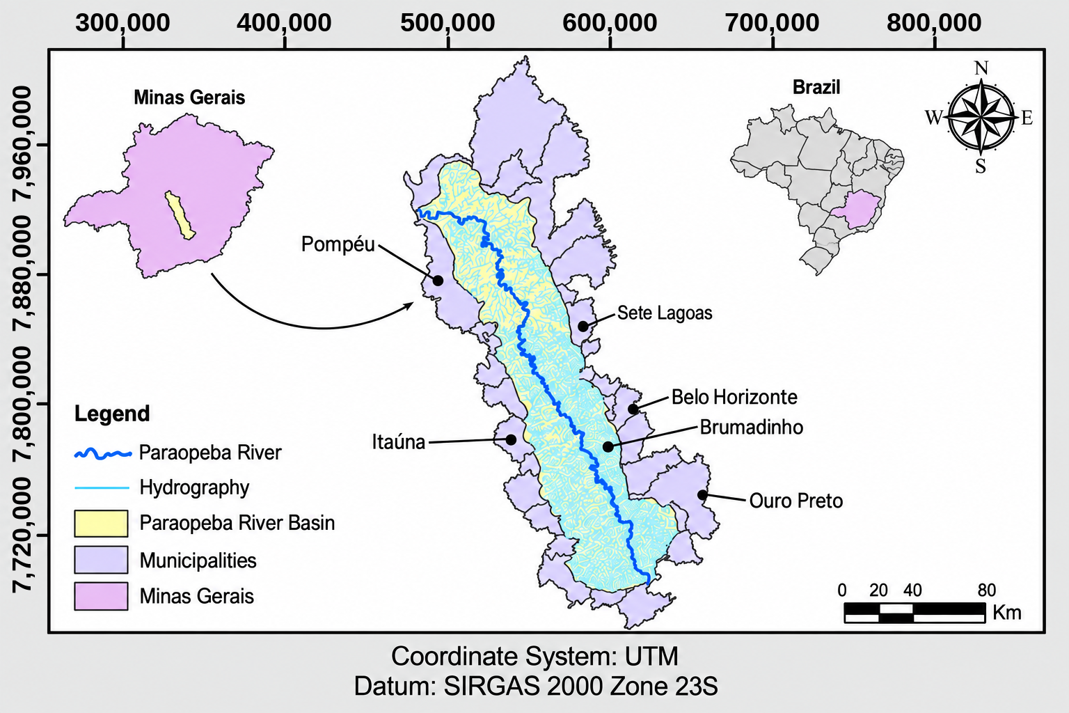
To apply and evaluate the proposed methodology, the Paraopeba River Basin (Figure 2) was selected. It is an important sub-basin of the São Francisco River Basin and is in the central region of Minas Gerais State, near the Metropolitan Region of Belo Horizonte (RMBH), Brazil.
The Paraopeba River basin has a drainage area of approximately 12,054 km2 and encompasses 48 municipalities in the state of Minas Gerais. The main water uses within the Paraopeba River basin include hydropower generation, public water supply, and industrial supply, particularly for mining and irrigation [18].
The basin supplies around 5.15 million inhabitants in the Metropolitan Region of Belo Horizonte (RMBH) and contains three major water-supply reservoirs: the Manso River (Manso), the Juatuba Stream (Serra Azul), and the Betim River (Várzea das Flores). Additionally, for electricity generation, the Paraopeba River basin hosts the Salto do Paraopeba and Retiro Baixo hydropower plants, as well as the level-control dam of the Igarapé thermoelectric plant, and it drains into the Três Marias reservoir [18].
Land use and land cover in the Paraopeba River basin are highly diverse, including agricultural and livestock activities (predominantly cattle ranching), mining, sand and clay extraction, and automotive industries. The basin is one of the most economically important regions in the state of Minas Gerais and includes the second-largest industrial hub in Brazil [19].
Figure 1.
Flowchart of the methodological framework for agricultural potential classification. Arrows indicate the sequence of steps; orange boxes indicate the sensitivity, uncertainty, and evaluation analyses.
The economic dynamics of the Paraopeba River basin are also diverse, with activities spanning all three economic sectors (primary, secondary, and tertiary). Within the primary sector, agro-silvo-pastoral activities play a crucial role in the region.
The basin has tropical climates with a dry winter (Köppen Aw and Cwa, with Cwb in the highest areas of the Upper Paraopeba) [20], with a rainy season from October to March. Elevations range from about 570 m at the Três Marias reservoir to more than 1500 m in the ranges of the Quadrilátero Ferrífero in the Upper Paraopeba. The main soil groups are Latosols (Oxisols), Cambisols (Inceptisols), Argisols (Ultisols), and Litholic Neosols (Entisols) [21] (Appendix A). Agricultural systems include extensive pastures for beef and dairy cattle (40.8% of the basin), eucalyptus plantations (5.3%), irrigated grain and vegetable crops, notably center-pivot systems in the Lower Paraopeba, and horticulture in the green belt of the RMBH. The main land-use pressures are urban and industrial expansion around the RMBH, iron-ore mining in the Quadrilátero Ferrífero, and the restrictions on water use that followed the 2019 failure of the B1 tailings dam in Brumadinho [22].
Figure 2.
Study area: Paraopeba River Basin, Minas Gerais, Brazil.
2.2. Selection and Preparation of Agricultural Potential Criteria
Selecting appropriate criteria is a fundamental step that must be aligned with the representation of the desired phenomenon and with data availability [23,24,25]. Numerous criteria influence the agricultural potential of a region; however, it is necessary to evaluate which criteria have available and open-access databases, and among these, select those that are most representative and not correlated with one another [13], since the use of a large number of criteria makes the analysis more complex and difficult [1,2].
The methodology proposed in the present study to identify areas with higher agricultural potential uses the following variables as criteria: land-use capability class, simplified climatic water balance, agricultural production value per hectare, and distance to roads.
This study aimed to identify agricultural potential in a general sense, without considering any specific crop. Criteria were therefore retained only when they (i) represented a constraint relevant to most agricultural uses, (ii) were available as open-access, spatially continuous data for the entire basin, and (iii) were not redundant with other criteria [1,2,13]. Soil chemical properties (e.g., pH, base saturation, and available phosphorus) were not included because acidity and low fertility, which prevail in the highly weathered soils of the basin, are routinely corrected through liming and fertilization, and because no spatially continuous soil chemical dataset compatible with the scale of the analysis is available [3,16]. Soil physical and morphological limitations that cannot be easily corrected—such as effective depth, drainage, stoniness, and susceptibility to erosion—were incorporated through the land-use capability classification (Section 2.2.1). Air temperature was not used because thermal requirements are crop-specific and because the basin lies within tropical climates with a dry winter (Köppen Aw and Cwa, with Cwb in the highest areas of the Upper Paraopeba) [20], in which temperature does not constrain most tropical crops and pastures. Irrigation accessibility and proximity to water resources were not used because the objective was to assess potential under rainfed conditions and because access to irrigation water depends on water-use permits and reservoir operation, which cannot be predicted spatially from the available data. The possible influence of these exclusions on the classification is discussed in Section 4.5. The four selected criteria were considered representative of agricultural potential across the diverse landforms and agricultural systems of the basin because each represents a distinct and spatially variable driver: land-use capability captures soil and terrain limitations across landforms, the CWB captures the climatic gradient between the Upper and Lower Paraopeba, the production value captures differences among regional agricultural systems, and distance to roads captures access to markets and inputs.
Although precipitation is considered in other studies [4,13], it was not used as an isolated variable in this study; instead, it was incorporated through the simplified climatic water balance (CWB), which is described in more detail in Section 2.2.2.
The following subsections describe the methodological procedures used to obtain the selected criteria, as well as the area used to apply the proposed methodology.
2.2.1. Land-Use Capability Classification
The classification of areas according to their land-use capability was based on the criteria presented by Rio Grande do Sul [26] and Lepsch et al. [7], who adapted the system proposed by the United States Department of Agriculture (USDA) [27] to Brazilian soils and climate. The apparent fertility criterion was not considered, since in conservationist/agricultural planning this parameter can be corrected through management practices [16,17]. Table 1 presents the eight land-use capability classes as proposed by Lepsch et al. [7]. Soil data were obtained from the Soil Map of Minas Gerais State [21], and the classification of the main soil component of each mapping unit is provided in Appendix A.
Table 1.
Description of land-use capability (LCC) classes.
The slope map was generated from the hydrologically conditioned digital elevation model (HCDEM) of the study basin and reclassified according to the eight land-use capability classes presented in Table 2. The HCDEM was derived from the NASADEM digital elevation model with a 30-m resolution [28].
Table 2.
Slope intervals assigned to land-use capability classes.
The final land-use capability class of each pixel was obtained by combining the soil-based and slope-based classes according to the principle of the most limiting factor [7,26]; that is, each pixel was assigned the more restrictive (higher) of the two classes. The soil-based class was defined for the main component of each soil mapping unit (Appendix A), considering the soil limitations that cannot be readily corrected by management—effective depth, drainage, stoniness or rockiness, and erodibility—following Lepsch et al. [7]. Accordingly, deep and well-drained Latosols (Oxisols) were assigned to Class II; Argisols (Ultisols), which have a textural gradient and higher erodibility, to Class III; Cambisols (Inceptisols) and Plinthosols, which are shallow or poorly structured and highly erodible in the basin [29], to Class VII; and Litholic and Quartzarenic Neosols and Gleysols, which have shallow depth, very low water retention, or permanent waterlogging, to Class VIII. For example, a pixel on a Latosol with a 12% slope was assigned to Class IV (slope-limited), whereas a pixel on a Cambisol with a 4% slope was assigned to Class VII (soil-limited). Because no soil unit was assigned to Class I, the final classes ranged from Class II to Class VIII. Land-use and land-cover (LULC) data were not used to define land-use capability; they were used only to allocate the economic criterion (Section 2.2.3) and to describe the correspondence between agricultural potential and current land use (Section 3.3).
The assignment of the soil-based classes followed the limitations that determine land-use capability in the system of Lepsch et al. [7]—effective depth, internal drainage, stoniness and rockiness, and susceptibility to erosion—and the erodibility (PKS) and water-recharge potential (PRHS) weights previously derived for the soils of the region [29] (Appendix A, PKS and PRHS). Latosols are deep, well drained, and the least erodible soils of the basin (PKS = 1.0–1.9), whereas Cambisols and Litholic Neosols have a shallow solum and the highest erodibility (PKS = 3.1–4.3 and 4.7–5.0, respectively). In the basin, Cambisols occur mainly on dissected landforms and are frequently associated with Litholic Neosols (Appendix A), which justified their assignment to Class VII, in which intensive annual cropping is not recommended without restrictions [7]. Because this is the most consequential assignment of the classification, its influence on the results was tested in the uncertainty analysis (Section 2.4).
2.2.2. Simplified Climatic Water Balance
Water availability is an essential factor for agricultural development. The simplified climatic water balance (CWB) is used to determine areas with water surplus, as shown in Equation (1). To compute the CWB, precipitation (input) and evapotranspiration (output) data were considered [30].
where CWB = simplified climatic water balance (mm yr−1); P = mean annual precipitation (mm yr−1); ET = mean annual actual evapotranspiration (mm yr−1).
Precipitation and evapotranspiration data were obtained from two gridded datasets for the period from 2000 to 2022. Evapotranspiration corresponds to the actual evapotranspiration of the Moderate Resolution Imaging Spectroradiometer (MODIS) product MOD16A3GF Version 6.1 (500 × 500 m) [31], which is estimated from remotely sensed vegetation data and meteorological data using the Penman–Monteith approach; it is therefore actual, not reference or potential, evapotranspiration. Precipitation data were obtained from the TerraClimate dataset (monthly data, 4 × 4 km) for the same period [32].
For each pixel, monthly TerraClimate precipitation was summed to obtain annual totals, and annual CWB values were calculated as the difference between average annual precipitation and average annual evapotranspiration considering the period from 2000 to 2022. Pixels without valid MODIS evapotranspiration values (urban areas and water bodies, which are flagged as fill values in the product) were excluded, consistent with the exclusion of these land covers from the analysis. Because actual evapotranspiration was used, the CWB represents the long-term water surplus (i.e., the water potentially available for runoff and groundwater recharge) under the current vegetation cover. Negative values indicate that, on average, evapotranspiration exceeds precipitation, a condition that can be sustained only by soil water storage, groundwater, or irrigation. The annual time step does not represent the seasonal water deficit of the dry season (approximately April to September), which affects rainfed agriculture throughout the basin; the CWB was therefore used as a relative indicator of water availability among areas, and its implications are discussed in Section 4.2. Regarding units and spatial alignment, MOD16A3GF annual ET values (kg m−2 yr−1, scale factor 0.1) were converted to mm yr−1 (1 kg m−2 = 1 mm), and TerraClimate precipitation (mm month−1) was summed to mm yr−1. The 2000–2022 means were computed for each dataset at its native resolution; both mean layers were then projected to SIRGAS 2000/UTM zone 23S, resampled by bilinear interpolation to the common 30 m grid (Section 2.2.5), and subtracted pixel by pixel. The CWB is therefore expressed in mm yr−1.
Actual rather than reference evapotranspiration was used because the purpose of the criterion is to represent the water that remains available in the landscape for runoff, groundwater recharge, and use under the current vegetation, as in previous prioritization studies in the region [29,30], rather than the atmospheric demand alone. Because this choice makes the criterion partly dependent on land cover, an alternative CWB based on reference evapotranspiration (P − PET), calculated with TerraClimate precipitation and Penman–Monteith reference evapotranspiration for the same period (2000–2022) [32], was evaluated in the uncertainty analysis (Section 2.4).
2.2.3. Agricultural Production Value per Hectare
To obtain the agricultural production value per hectare variable, three different datasets were used, one for each type of agricultural activity present in the Paraopeba River basin: the Production of Plant Extraction and Planted Forests [33] and the Municipal Agricultural Production datasets for Temporary Crops [34] and Permanent Crops [35]. These datasets contain the value of agricultural production and the area allocated for harvesting for each municipality for the year 2022.
Although the Paraopeba River Basin officially comprises 48 municipalities, the spatial intersection between the municipal boundaries and the delineated basin polygon identified additional municipalities with small portions of their territories within the basin. These municipalities were retained in the analysis because their intersecting areas were included in the spatial allocation of agricultural production values.
The agricultural production value per hectare for each municipality was calculated by dividing the sum of the production values of the three datasets by the sum of the corresponding harvested areas (or areas allocated to harvest) in each municipality. Each activity is thus weighted by its harvested area, and the indicator represents the gross value of agricultural production per harvested hectare, not net income, profit, or physical land productivity. This methodology was also used by Marcos-Martinez et al. [10] to determine commercial prices for the sale of cereals and livestock, based on data from 1992–2010. Agricultural production values per hectare for each type of production and their corresponding areas are presented in Appendix B.
LULC data were obtained from the MapBiomas platform for the year 2022 [36] and reclassified into six LULC classes, as presented in Appendix C.
The agricultural production value per hectare for each municipality was assigned to areas whose LULC corresponded to agricultural use (pasture, temporary crops, permanent crops, and planted forests). For areas where LULC corresponded to forest land or natural non-forest formation, an agricultural production value per hectare of R$0.00 was assigned, as these areas are not considered productive. Areas that do not fall within the scope of this study—such as non-vegetated areas and water bodies—were excluded from the analysis. Pasture areas received the municipal value because the surveys used do not report livestock production values per hectare.
This procedure assumes that the production value per hectare is spatially uniform within each municipality. Municipal statistics were used because they are the finest-scale official economic data available for all crops and planted forests in Brazil, and the criterion was intended to represent the regional economic context of agriculture rather than the productivity of individual fields. The implications of this assumption are discussed in Section 4.3, and the influence of the economic criterion on the classification was evaluated through the sensitivity analysis, including a scenario in which this criterion was removed (Section 2.4).
2.2.4. Distance to Roads
Considering that roads contribute to the development of the agricultural and forestry sectors by facilitating access and transportation of production [37,38], it was assumed that the shorter the distance to roads, the greater the agricultural potential.
Distance to roads was determined using the Euclidean distance from each pixel to the nearest road. State and federal road networks were obtained from MapBiomas [39].
2.2.5. Spatial Data Processing
Before the multicriteria analysis, all spatial datasets were prepared to ensure compatibility among the criteria. The datasets were processed in ArcGIS 10.3 (Esri, Redlands, CA, USA) and QGIS 3.22 (QGIS Development Team, Open Source Geospatial Foundation, Laax, Switzerland) using the SIRGAS 2000/UTM Zone 23S coordinate reference system. Raster layers with different native spatial resolutions were resampled to a common spatial resolution of 30 m. Continuous variables were resampled using bilinear interpolation, whereas categorical variables were resampled using the nearest-neighbor method. All layers were aligned to the same spatial extent and pixel grid before standardization and integration through the Weighted Linear Combination (WLC). The final agricultural potential map was generated at a spatial resolution of 30 m.
Resampling to 30 m does not increase the information content of the coarser datasets (MODIS, 500 m; TerraClimate, ~4 km; municipal statistics). It was adopted only to provide a common analysis grid matching the resolution of the slope and LULC data, which carry the finest spatial detail. Consequently, the CWB and economic criteria represent regional gradients, and local variations in agricultural potential within a single MODIS or TerraClimate cell are driven mainly by land-use capability and distance to roads. The final map should therefore be interpreted at the basin or regional planning scale and not at the farm scale. In addition, because the economic criterion is constant within each municipality, it introduces abrupt changes in the index at municipal boundaries that do not correspond to actual changes in agricultural conditions. These effects mainly influence the position of class boundaries rather than the general spatial pattern, because the finest-resolution criterion (land-use capability) accounts for more than half of the weights.
2.3. Multicriteria Analysis
For the multicriteria analysis, the weighted linear combination (WLC) technique was applied, in which the criteria were rescaled and weighted based on a set of weights that enabled the hierarchical ordering of the criteria [40,41]. For rescaling continuous variables, the fuzzy concept was used, which considers the differences within each factor and assumes a mathematical distribution function that best explains the variation in the factor [42]. Rescaling was performed on a scale from 0 to 1, following a linear function for all criteria, with the convention that higher values represent greater suitability of the criterion for the intended objective. The ordinal LCC criterion was converted to scores using the same decreasing linear function (Class II = 1.00; III = 0.83; IV = 0.67; V = 0.50; VI = 0.33; VII = 0.17; VIII = 0.00).
The definition of weights for each factor in the multicriteria analysis followed the methodology proposed by Thomas Saaty [43], which is based on pairwise comparison of criteria using the Analytic Hierarchy Process (AHP) [44]. This approach reduces interpretation subjectivity and increases confidence in the results and decision-making process [45,46].
To define the weights, a pairwise comparison matrix was used [42,47]. To construct this matrix, the criteria were ranked based on their relative importance to the final objective [48].
In the AHP analysis, the criteria are compared with one another, and weights are assigned to each comparison based on their importance for the phenomenon being studied. The weight values range from 1 to 9, where 1 indicates equal importance and 9 indicates extreme importance [45,49], as shown in Table 3 [45,49].
Table 3.
AHP scale for assigning weight values.
Based on this scale, the pairwise comparison matrix adopted in this study was constructed as shown in Table 4.
Table 4.
Pairwise comparison matrix and resulting weights of the agricultural potential criteria (λmax = 4.117; CI = 0.039; RI = 0.90; CR = 0.043).
The pairwise judgments were established by consensus among the six authors, who have experience in soil and water conservation, hydrology, and agricultural planning in the region. The criteria were first ranked according to their role in the definition of agricultural potential, and the intensity of each comparison was then agreed on the basis of the relative importance given to equivalent criteria in previous GIS–AHP land-suitability studies, in which soil and terrain criteria usually receive the largest weights, followed by climatic water availability and by socioeconomic and accessibility criteria [2,3,11,13]. LCC was considered the most important criterion because it synthesizes the permanent soil and terrain limitations that cannot be easily removed by management and that determine the sustainability of agricultural use [7]. LCC was judged moderately (intensity 3), rather than strongly, more important than CWB because both criteria express biophysical constraints, but the limitations represented by LCC (shallow soils, erodibility, and slope) are permanent, whereas water deficits can be partly mitigated by irrigation and water-conservation practices. CWB was ranked second because water availability is a primary constraint on rainfed production [4,13]. Agricultural production value per hectare was ranked third because it reflects current economic conditions, which are more variable over time than the biophysical criteria. Distance to roads was ranked last because the basin is well served by roads (Section 3.1), so accessibility differentiates areas less than the other criteria [38]. Because these judgments are inevitably subjective, their uncertainty was evaluated by Monte Carlo simulation (Section 2.4).
After assigning the weights, the consistency of the pairwise comparisons was evaluated using the consistency ratio (CR), which ranges from 0 to 1. CR values lower than 0.10 are considered acceptable [45,46]. The weights were calculated as the normalized principal eigenvector of the matrix, and the CR was obtained as CR = CI/RI, where CI = (λmax − n)/(n − 1) is the consistency index, λmax is the principal eigenvalue, and RI is the random index (0.90 for n = 4) [43,46]. For the matrix in Table 4, λmax = 4.117, CI = 0.039, and CR = 0.043 (4.3%), and the normalized weights are 0.565 (LCC), 0.262 (CWB), 0.118 (agricultural production value per hectare), and 0.055 (distance to roads), which sum to 1.000 (Table 4). The approximate method of averaging the normalized columns of the matrix gives weights that differ by less than 1 percentage point.
The standardized criteria were integrated using the Weighted Linear Combination (WLC) method, according to Equation (2):
where AP is the agricultural potential index, wi is the weight assigned to criterion i through the Analytic Hierarchy Process (AHP), xi is the standardized value of criterion i on the fuzzy scale, and n is the total number of criteria. The weights were normalized so that their sum was equal to 1. Therefore, criteria with greater relative importance had a greater influence on the final agricultural potential index.
Once the criteria were integrated to obtain the agricultural potential map, the resulting raster was categorized into five potential classes: very low, low, moderate, high, and very high. The natural breaks (Jenks) classification method, available in ArcGIS, was used for categorization; this method defines class limits that minimize the variance within classes and maximize the variance between classes, and it is widely applied in thematic cartographic analyses [50]. The resulting class limits were 0.260, 0.390, 0.540, and 0.660.
2.4. Sensitivity Analysis and Evaluation of the Results
The robustness of the agricultural potential classification to the AHP weights was evaluated in two complementary ways. First, a judgment-level analysis was performed by changing each of the six pairwise judgments in Table 4 by one step on the Saaty scale (upward and downward), recalculating the weights and the CR, and verifying whether the ranking of the criteria changed. Second, a spatial one-at-a-time (OAT) sensitivity analysis was performed [14,15]: the weight of each criterion was varied by ±10%, ±20%, and ±30% of its original value, and the weights of the remaining criteria were rescaled proportionally so that their sum remained equal to 1, resulting in 24 scenarios (Appendix D). In addition, three alternative scenarios were tested: (S1) equal weights (0.25 each); (S2) a biophysical-only scenario, in which the economic criterion was removed and the remaining weights were renormalized (LCC = 0.641, CWB = 0.297, distance to roads = 0.062); and (S3) a scenario with reduced dominance of LCC (LCC = 0.40, CWB = 0.30, agricultural production value per hectare = 0.20, distance to roads = 0.10). For each scenario, the agricultural potential index was recalculated and classified using the same class limits, and the results were compared with the baseline map in terms of the area of each class, the percentage of the basin that retained its class, the percentage of pixels that shifted by more than one class, and the Spearman correlation coefficient (ρ) between the continuous indices.
Because the economic criterion uses LULC to allocate production values (Section 2.2.3), comparisons between the agricultural potential map and current LULC are not independent of the model. Therefore, the correspondence between agricultural potential and current land use (Section 3.3) is reported only as descriptive spatial agreement. To reduce this circularity, the index of the biophysical-only scenario (S2), which does not use the economic criterion, was compared with the agricultural land use mapped in 2022 (pasture, temporary and permanent crops, and planted forests) versus forest and natural non-forest formations, using the area under the receiver operating characteristic curve (AUC). In all scenarios, the class limits of the baseline map were kept fixed, so that changes in class reflect only the changes in the weights.
To address uncertainty beyond the criterion weights, three additional analyses were performed. First, the uncertainty of the expert judgments was propagated by Monte Carlo simulation [49]: 1000 pairwise comparison matrices were generated by randomly changing each of the six judgments of Table 4 by up to one step on the Saaty scale (moderate uncertainty) and, in a second set of 1000 matrices, by up to two steps (high uncertainty, which allows the ranking of the criteria to be reversed); only matrices with CR ≤ 0.10 were retained. For each pixel, the percentage of simulations in which it retained its baseline class was calculated. Second, the main methodological choices were changed one at a time: (i) limits of the fuzzy functions at the 2nd and 98th percentiles instead of the minimum and maximum; (ii) sigmoidal instead of linear fuzzy functions; (iii) CWB without the truncation of deficits to zero; (iv) CWB calculated with reference evapotranspiration (P − PET); (v) activity-specific allocation of the production value, in which pixels of temporary crops, permanent crops, and planted forests received the municipal value per hectare of the corresponding activity; (vi) reassignment of the soils assigned to Class VII to Classes VI or V, applied to all Class VII pixels as an upper-bound test and, in a second test, only to the Class VII pixels with slope below 20% (30 m slope map derived from the NASADEM-based HCDEM [28]; Section 2.2.1); (vii) classification by equal intervals or quantiles instead of natural breaks; and (viii) calculation of the index at a resolution of 480 m (blocks of 16 × 16 pixels), compared with the majority class of the 30 m map. The results were compared with the baseline map using the percentage of the basin that retained its class, the percentage of high- and very high-potential areas retained, and the Jaccard index between the high- and very high-potential areas of the two maps. Third, the contribution of each criterion to the spatial variation in the index was quantified by the share of the variance of the index that occurs between land-use capability classes and by the change in the classification when each criterion was removed.
Finally, to support the interpretation of the results for planning, the agricultural potential classes were combined with LULC in 2022 [36] into five planning classes: agricultural land (pasture, crops, and planted forests) with high or very high potential, agricultural land with moderate potential, agricultural land with low or very low potential, native vegetation (forest and natural non-forest formations), and urban areas, mining, and water bodies.
The sensitivity and uncertainty analyses were performed in Python 3 (Python Software Foundation, Wilmington, DE, USA) with the NumPy and SciPy libraries (Scripts S1 and S2).
3. Results
3.1. Spatial Distribution of the Criteria
Figure 3 presents the spatial distribution maps of the criteria used to develop the agricultural potential map for the Paraopeba River basin: land-use capability classification (Figure 3a), simplified climatic water balance (Figure 3b), agricultural production value per hectare (Figure 3c), and distance to roads (Figure 3d).
Figure 3.
Criteria used to generate the agricultural potential map for the Paraopeba River basin: (a) Land-use capability classification. (b) Simplified climatic water balance. (c) Agricultural production value per hectare. (d) Distance to roads.
In the Paraopeba River basin, land-use capability classes range from Class II to Class VIII, with a predominance of Classes IV and VII, which are typically assigned to pasture and planted forests. Pasture (40.8%) and planted forests (5.3%), uses compatible with these classes, together occupy 46.1% of the basin, indicating an overall correspondence between current land use and land-use capability.
The classes assigned to intensive cultivation (Classes II and III) represent 21.8% of the basin, predominantly in the Lower Paraopeba region near the basin outlet. This region is characterized by Oxisols, which are well-structured, deep soils with generally high infiltration capacity [29], favoring agricultural use.
In the Upper Paraopeba region—a mountainous area—the main limiting factor for land use is slope. This region contains Neosols, which have high erodibility, and igneous rocks with low porosity. Combined with steep slopes, these conditions increase soil loss and promote the occurrence of rocky outcrops. Additionally, this region exhibits high water surplus due to high precipitation and low evapotranspiration.
In the Lower Paraopeba region, the main limiting factor for land-use capability is soil. Some portions of this region are dominated by Cambisols, which have low infiltration potential.
The second criterion analyzed was the simplified climatic water balance (CWB). Overall, the Paraopeba River Basin contains a larger proportion of areas with water surplus than with water deficit. Positive CWB values indicate greater climatic water availability and may therefore favor agricultural production.
Despite this overall predominance of water surplus, water-deficit areas are concentrated mainly in other portions of the Lower Paraopeba region. These areas coincide with LCC classes indicating suitability for intensive cultivation (Classes II and III).
Areas with the highest water surplus coincide with LCC Classes VII and VIII, which are assigned to pasture and conservation areas, respectively. These areas correspond to regions with high precipitation and low-canopy vegetation, which together lead to higher CWB values.
Regarding agricultural production value per hectare, the municipality of Caetanópolis recorded the lowest value in 2022 (BRL 3251.77 ha−1), with permanent crops showing the highest agricultural production values per hectare. In contrast, the municipality of Pequi showed the highest agricultural production value per hectare (BRL 62,029.17 ha−1), with temporary crops showing the highest agricultural production value per hectare. The mean agricultural production value per hectare of the municipalities in the Paraopeba River basin was BRL 15,225.08 ha−1, with permanent crops showing the highest mean value (BRL 27,525.86 ha−1), followed by temporary crops (BRL 19,585.34 ha−1) and plant extraction and planted forests (BRL 5289.54 ha−1) (Appendix B).
The distance-to-roads criterion was used to evaluate ease of production transport and access to properties. Most of the Paraopeba River basin is located less than 2 km from major roads. Greater distances occur mainly in areas classified as natural non-forest formation, planted forest, or forest, whereas the shortest distances are found in areas where LULC corresponds to pasture, temporary crops, or permanent crops.
3.2. Criterion Weights and Standardization
Table 5 presents the criteria used in the multicriteria analysis, as well as the rescaling functions, threshold values, and weights obtained through the AHP analysis.
Table 5.
Criteria, functions, and weights assigned for identifying the agricultural potential of the Paraopeba River basin.
The histograms did not indicate the need to exclude extreme values; therefore, the full observed ranges were used for standardization. For the CWB criterion, only areas with water surplus were considered to have agricultural potential. A value of zero was assigned to all areas with water deficit; thus, only positive values were used. This zero value applies only to the CWB score and not to the final index: pixels with water deficit can still reach an agricultural potential index of up to 0.738 and be classified as high or very high potential, depending on the other criteria.
3.3. Agricultural Potential
Figure 4 shows the spatial variability of agricultural potential (Figure 4a) and the LULC distribution for the Paraopeba River basin (Figure 4b).
Figure 4.
Identification of agricultural potential (a) and land use and land cover (LULC) for the year 2022 (b) in the Paraopeba River basin. VL = Very low agricultural potential; L = Low agricultural potential; M = Moderate agricultural potential; H = High agricultural potential; VH = Very high agricultural potential. Source: (a) Authors; (b) adapted from MapBiomas [36].
In the Paraopeba River basin, the most frequent classes are low (26.4%) and high (27.2%) agricultural potential, totaling 53.6% of the basin area. Areas with high agricultural potential are predominantly located in the Lower Paraopeba region. This region is characterized by low slopes, a predominance of Oxisols, and good water availability, including both surface water and groundwater [51], which favors agricultural development.
Some areas in the Lower Paraopeba show low or very low agricultural potential. These correspond to regions with Cambisols where LULC is dominated by natural non-forest formations.
Areas with moderate agricultural potential are mainly found in the Middle Paraopeba and in the Upper Paraopeba on the left bank of the river. In these regions, predominant LULC corresponds to pasture, permanent crops, and forested areas.
On the right bank of the Upper Paraopeba, including the Serra da Calçada, areas are classified as having low or very low agricultural potential. These regions exhibit the highest slopes, the lowest CWB values, and the lowest infiltration potential.
As shown in Table 5, land-use capability is the most influential criterion. Therefore, areas with high and very high agricultural potential coincide with LCC Classes II and III, while areas classified as low or very low potential overlap with LCC Classes VII and VIII.
In the Lower Paraopeba, although some areas belong to LCC Class II, not all have very high agricultural potential; these areas exhibit water deficit, which reduced their potential from very high to high. A similar pattern is observed on the right bank of the Upper Paraopeba, where areas classified as LCC Class VII correspond to low and very low agricultural potential and also exhibit water deficit.
Table 6 presents the percentage of each LULC class for the year 2022 [36] within each agricultural potential class in the Paraopeba River basin. These values describe the spatial correspondence between the model output and current land use and do not constitute an independent validation, because LULC was used to allocate the economic criterion (Section 2.2.3).
More than two-thirds (69.7%) of forest areas fall within the very low to moderate potential classes, and 57.5% of natural non-forest formations (including wetlands, marshes, grassland formations, and rocky outcrops) are located in low-potential areas.
Some discrepancies between the agricultural potential map and current LULC can be observed. The low-potential class contains 30.7% of the temporary crop areas in the basin, particularly concentrated in the Lower Paraopeba.
Regarding permanent crops, 31.6% and 43.5% occur in high and very high agricultural potential areas, respectively. Appendix B presents the agricultural production value per hectare for each crop type by municipality. The municipality of Paraopeba recorded the highest agricultural production value per hectare for permanent crops and is located in an area with high to very high agricultural potential. Conversely, Resende Costa, located in the Upper Paraopeba on the left bank, recorded the lowest agricultural production value per hectare for permanent crops, with most cultivated areas located in low and very low potential zones.
Table 6.
Percentage of each LULC class by agricultural potential class in the Paraopeba River basin.
The municipality of Pequi recorded the highest overall agricultural production value per hectare, with temporary crops showing the highest agricultural production values per hectare. The cultivated areas in Pequi coincide with very high agricultural potential zones. In São Joaquim de Bicas, the municipality with the second-highest agricultural production value per hectare, a similar pattern was observed.
3.4. Sensitivity Analysis
Changing each pairwise judgment in Table 4 by one step on the Saaty scale did not change the ranking of the criteria in any of the 12 cases, and all modified matrices remained consistent (CR between 2.8% and 8.9%). The weights varied from 45.3% to 61.9% for LCC, from 20.5% to 36.3% for CWB, from 9.0% to 15.8% for agricultural production value per hectare, and from 4.9% to 7.3% for distance to roads. The largest changes occurred when the judgment between LCC and CWB was modified (from 3 to 1 or 5), indicating that the relative importance of these two criteria is the most influential judgment in the matrix.
In the spatial OAT analysis, 85.6–98.4% of the basin retained its baseline class under ±10% weight variations and 71.7–96.9% under ±20% variations (Table 7). The classification was most sensitive to the weight of LCC and least sensitive to the weight of distance to roads. Shifts of more than one class affected at most 0.4% of the basin (under a 30% reduction in the LCC weight) and did not occur in any of the other scenarios, and the Spearman correlation between the baseline and modified indices was ≥ 0.975 in all OAT scenarios. Under ±20% variations, at least 83.4% of the pixels classified as high or very high potential in the baseline remained in these classes.
Table 7.
Percentage of the basin area that retained the baseline agricultural potential class under one-at-a-time variations of the criterion weights (weights of each scenario are given in Table A4).
Among the alternative scenarios (Table 8), equal weights (S1) produced the largest change: only 34.0% of the basin retained its class, the moderate class increased from 13.5% to 46.5%, and the very high class decreased from 19.5% to 3.4%, because the lower weight of LCC compressed the index toward intermediate values. Removing the economic criterion (S2) maintained the class of 72.7% of the basin and 99.8% of the high- and very-high-potential areas, whereas the very high class increased to 32.5%. Reducing the dominance of LCC (S3) maintained the class of 62.3% of the basin and 72.0% of the high- and very-high-potential areas. The Spearman correlation with the baseline index was ≥ 0.879 in all scenarios.
Table 8.
Weights, area of each agricultural potential class, percentage of the basin that retained the baseline class, and Spearman correlation (ρ) with the baseline index for the alternative weighting scenarios (class limits of the baseline map kept fixed).
Land-use capability accounted for most of the spatial variation of the index: 94.4% of its variance occurred between capability classes, and the other criteria determined the class of each pixel only within the range allowed by its capability class. For example, 56.8% of the Class III pixels were classified as high and 39.0% as very high potential, and 67.4% of the Class VII pixels were classified as low and 32.5% as very low potential. Because CWB was negatively correlated with LCC (r = −0.21), its net contribution to the variance of the index was small; nevertheless, removing it changed the class of 43.1% of the basin, mostly between adjacent classes, whereas 99.7% of the high- and very high-potential areas remained in these classes.
In the Monte Carlo analysis with moderate uncertainty, LCC remained the most important criterion in 93.8% of the 1000 consistent matrices, and the 5th–95th percentile ranges of the weights were 0.40–0.65 for LCC, 0.16–0.42 for CWB, 0.07–0.21 for agricultural production value per hectare, and 0.04–0.10 for distance to roads. On average, pixels retained their baseline class in 79.2% of the simulations, 62.1% of the basin retained its class in at least 75% of the simulations, and pixels classified as high or very high potential remained in these classes in 91.6% of the simulations (Figure 5a). The least stable areas were located mainly in the Lower Paraopeba, near the limits between classes. Under high uncertainty, which allowed the ranking of the criteria to be reversed, LCC remained the most important criterion in 75.2% of the simulations, pixels retained their class in 64.5% of the simulations, and high- and very high-potential pixels remained in these classes in 79.5% of the simulations.
Figure 5.
(a) Percentage of the 1000 Monte Carlo simulations of the AHP judgments (moderate uncertainty, ±1 step on the Saaty scale) in which each pixel retained its baseline agricultural potential class; (b) planning classes obtained by combining agricultural potential with land use and land cover in 2022. Source: (b) adapted from MapBiomas [36].
Among the methodological alternatives (Table 9), the high- and very high-potential areas were most robust to the activity-specific allocation of the production value, to the reassignment of the Class VII soils, and to the sigmoidal functions (Jaccard index ≥ 94.9%), whereas the alternatives that changed the range of the standardized criteria (percentile limits and CWB without truncation) or the CWB formulation (P − PET) changed the class of 31.6–39.3% of the basin, mainly between adjacent classes, but retained 93.2–100% of the high- and very high-potential areas. The classification method had the largest effect on the class areas: with equal intervals from 0 to 1, the very high class covered only 0.6% of the basin, which confirms that the class labels are relative to the basin. The index calculated at 480 m agreed with the majority class of the 30 m map in 80.2% of the blocks and in 93.3% of the blocks for the distinction between high/very high and other classes.
Table 9.
Effect of alternative methodological choices on the agricultural potential classification, compared with the baseline map: percentage of the basin that retained its class, percentage of the high- and very high-potential (H/VH) areas retained, and Jaccard index between the H/VH areas of the two maps.
3.5. Agreement with Current Agricultural Land Use
When the index of the biophysical-only scenario (S2), which does not use the economic criterion, was compared with the agricultural land use mapped in 2022 (pasture, temporary and permanent crops, and planted forests, which occupy 72.3% of the analyzed area), the AUC was 0.63. For comparison, the AUC was 0.62 for the LCC criterion alone and 0.68 for the baseline index, which includes the economic criterion. Most of the area mapped as temporary crops corresponds to the MapBiomas class “mosaic of uses” (20.4% of the basin), in which agriculture and pasture cannot be separated, whereas annual crops mapped individually (sugarcane, soybean, and other temporary crops) occupy only 2.3% of the basin. These annual crops were concentrated in the high- and very high-potential classes (73.8%), and only 20.3% of them were in the very low and low classes, compared with 44.4% of the mosaic of uses. For annual and perennial crops mapped individually, the AUC of the land-use capability criterion alone, which is derived exclusively from soil and terrain data and is independent of LULC, was 0.63.
4. Discussion
4.1. Drivers of Agricultural Potential and Influence of the Criteria
Land-use capability was the main driver of the spatial pattern of agricultural potential, consistent with its weight (56.5%) and with previous studies. Ostovari et al. [11] also identified soil as the main determinant of suitable agricultural areas, and Tashayo et al. [3] and Han et al. [13] found that soil texture was the most important criterion, followed by slope. Soil and slope are the components of the land-use capability criterion, the most influential in this study. The inclusion of the simplified climatic water balance enabled areas with similar land-use capability to be differentiated according to hydroclimatic constraints, highlighting the importance of combining relatively stable soil and terrain characteristics with variables that represent climatic water availability when assessing agricultural potential.
Because the index is a weighted linear combination, the weights define the range of values that each LCC class can attain. Pixels in Classes II and III have a minimum index of 0.565 and 0.471, respectively, even when all other criteria are equal to zero, and therefore cannot be classified as low or very low potential. Conversely, pixels in Classes VII and VIII can reach at most 0.529 and 0.435, respectively, and therefore cannot be classified as high or very high potential, regardless of water availability, economic performance, or accessibility. The secondary criteria thus act mainly within each capability class. This behavior is consistent with the conservationist purpose of the framework, because intensive agricultural use is not recommended for land with severe permanent limitations [7], but it also means that the results depend strongly on the soil-based capability assigned to each soil mapping unit. In the flat areas of the Lower Paraopeba, for example, low potential can occur only on soil units assigned to Classes VII or VIII, mainly Cambisols (Appendix A), which explains why part of the temporary crops of this region falls into the low-potential class (Table 6). Because the soil map represents soil associations by their main component at a regional scale [21], part of these areas may include more favorable soils, and a more detailed soil survey could change their classification. Nevertheless, the sensitivity analysis (Section 3.4) indicated that the spatial pattern of agricultural potential is robust to moderate changes in the weights, since pixels almost never shifted by more than one class and the rank correlation with the baseline index remained ≥ 0.975.
The dominance of land-use capability is a deliberate consequence of the conservationist purpose of the framework and of the weights, but it has two implications. First, the index should be interpreted mainly as a refinement of land-use capability by climatic, economic, and accessibility conditions, rather than as an equal combination of the four criteria; the secondary criteria are decisive within capability classes, where they separate, for example, very high from high potential on Latosols. Second, the results depend on the expert judgments. Although the Monte Carlo analysis showed that the high- and very high-potential areas are stable under moderate uncertainty, it quantifies but does not remove the subjectivity of the initial weighting. When the framework is transferred to other watersheds, the weights should therefore be re-elicited with local experts and stakeholders and, where the purpose is to emphasize climatic or economic conditions, scenarios with a lower weight for land-use capability (such as S1 and S3; Table 8) should be considered.
In the Upper Paraopeba, the combination of high water surplus, steep slopes, and low infiltration potential may significantly contribute to surface runoff and erosion processes, increasing the vulnerability of the basin, and mining activities in this region may increase pollutant loads transported by surface runoff. Measures that enhance water infiltration and maintain soil cover are therefore needed, and Costa et al. [52] highlight that the presence of forested areas—especially near zones with high erosion potential—is essential for pollutant retention. Similarly, in the Lower Paraopeba, where Cambisols with low infiltration potential coincide with positive CWB values, measures that enhance water infiltration may be important to reduce surface runoff and improve water retention.
4.2. Climatic Water Balance, Water Deficit, and Irrigation
The predominance of water surplus in the basin is consistent with the findings reported by Coelho et al. [29]. The water-deficit areas of the Lower Paraopeba coincide with LCC Classes II and III, highlighting the spatial heterogeneity of the region and the importance of incorporating climatic conditions into the assessment, since land-use capability classification considers soil and terrain characteristics but does not explicitly account for climatic factors. Conversely, the highest water surpluses occur in LCC Classes VII and VIII, in areas with high precipitation and low-canopy vegetation. Forest structural attributes, such as canopy height and leaf area, strongly influence evapotranspiration, with more developed forest canopies generally associated with greater evapotranspiration [53].
Because the CWB was calculated with actual rather than reference evapotranspiration, it represents the long-term water surplus under the current land cover rather than a purely climatic index. Part of the water deficit detected in the Lower Paraopeba may therefore reflect the high evapotranspiration of irrigated crops, which is consistent with the extensive center-pivot irrigation in this region. As noted by Pacheco and Pissarra [51], groundwater contributions in this region may partly compensate for climatic water limitations and help explain the extensive irrigated agriculture observed there. In addition, the annual time step does not capture the seasonal deficit of the dry season, which affects rainfed agriculture throughout the basin. A monthly or crop-specific water balance based on reference evapotranspiration would better represent the timing of water stress and should be considered in future applications. The comparison with the reference-based CWB (P − PET) showed that the two formulations are only weakly correlated (Spearman ρ = 0.28) because the actual-evapotranspiration CWB is strongly influenced by vegetation and has a finer spatial resolution. However, the areas with water deficit in the actual-evapotranspiration CWB (1.5% of the basin) also had climatic deficits (mean P − PET = −216 mm yr−1, compared with +11 mm yr−1 in the basin), which indicates that they are not only an effect of irrigation. Replacing the CWB with P − PET changed the class of 39.3% of the basin but retained 93.2% of the high- and very high-potential areas (Table 9), so the identification of priority areas does not depend on the choice of evapotranspiration variable.
Areas with water deficit received a CWB score of zero because the index was designed to represent agricultural potential under rainfed conditions. This choice does not assign zero agricultural potential to these areas; it only removes the contribution of the CWB criterion, so that pixels with water deficit can still reach an index of up to 0.738 and be classified as high or very high potential when the other criteria are favorable, as observed in the Lower Paraopeba. Irrigation can compensate for climatic water deficits, but its feasibility depends on water availability, water-use permits, and investment capacity, which vary locally and could not be represented with the available data. Moreover, after the 2019 failure of the B1 tailings dam in Brumadinho, the use of raw water from the Paraopeba River was restricted along part of its course, and water quality deterioration persisted in the following years [22]. The potential of the water-deficit areas should therefore be interpreted as conditional on access to irrigation water.
The fact that 30.7% of the temporary cropland falls in the low-potential class (Table 6) results from the combination of several factors. First, most of this class corresponds to the mosaic of uses, which includes pasture; annual crops mapped individually were mostly in the high- and very high-potential classes (73.8%; Section 3.5). Second, land-use capability plays a major role: in the flat areas of the Lower Paraopeba, where most of these crops are located, low potential can occur only on soil units assigned to Classes VII or VIII, mainly Cambisols (Section 4.1). Third, these crops are largely irrigated, often by center pivots, and irrigation is not represented in the index; moreover, the high actual evapotranspiration of irrigated fields lowers the CWB. Fourth, the municipal economic data dilute the value of irrigated crops in municipalities of the Lower Paraopeba where pastures and silviculture predominate (e.g., Pompéu, Curvelo, and Felixlândia, with 3396–7245 BRL ha−1; Appendix B). The classification thresholds play a minor role: because Class VII pixels cannot exceed an index of 0.529, they cannot reach the high class (≥ 0.540) under any combination of the other criteria. Low potential therefore indicates that these crops depend on management inputs—irrigation and soil conservation—that compensate for permanent land limitations.
4.3. Economic Criterion, Spatial Agreement, and Evaluation of the Model
The spatial allocation of a single production value per hectare to all agricultural areas within each municipality assumes intra-municipal homogeneity of production systems. This assumption does not hold strictly in the basin, where irrigated systems, horticulture, and extensive pastures coexist within the same municipalities, and it may be particularly relevant for municipalities whose territories intersect only small portions of the basin. However, its effect on the results is limited by the low weight of the criterion (11.8%). Within a municipality, the economic score is constant, so local differences in agricultural potential are driven by LCC, CWB, and distance to roads, whereas the economic criterion shifts the index of the agricultural areas of a municipality by at most 0.118. Moreover, when each agricultural pixel received the municipal value of its own activity (temporary crops, permanent crops, or planted forests) instead of the municipal average, the class of only 1.5% of the basin changed (Table 9), although the activity-specific values varied within municipalities (median coefficient of variation = 0.19). Accordingly, removing this criterion (S2) changed the class of 27.3% of the basin, although 99.8% of the high- and very-high-potential areas remained in these classes (Table 8). A further limitation is that the IBGE surveys used do not report production values for livestock, particularly beef and dairy cattle, so pasture areas received the municipal value of crops and planted forests. Future studies could use spatially explicit productivity indicators, such as remotely sensed vegetation indices [4], to represent intra-municipal variability.
The economic criterion also reflects the crop composition of each municipality, because production values and harvested areas were aggregated across temporary crops, permanent crops, and plant extraction and silviculture, so that each activity is weighted by its harvested area. Municipalities dominated by high-value horticulture or irrigated crops, such as Pequi, São Joaquim de Bicas, and Mário Campos, therefore show high values, whereas those dominated by silviculture and extensive systems show low values. Gross production value is not equivalent to profit or land productivity: it does not account for input costs, investments in irrigation, or farm size, and it depends on the commodity prices of 2022. The indicator should therefore be interpreted as a proxy for the regional economic intensity of agriculture rather than as a measure of profitability.
The correspondence between agricultural potential, current land use, and production values (Table 6 and Appendix B) must be interpreted with caution. Because LULC was used to allocate production values, and because actual evapotranspiration reflects the current vegetation cover, part of this agreement is built into the model and cannot be considered an independent validation. For example, forests and natural formations received an economic score of zero, which partly explains their concentration in the lower potential classes. When the economic criterion was removed (S2), the index still discriminated agricultural land from natural vegetation (AUC = 0.63). This moderate value reflects the fact that a large part of the pastures of the basin occupies land with severe capability limitations (32.2% of pasture areas are in the very low and low classes; Table 6). These results indicate that the agreement with current land use does not depend only on the economic criterion, but also that current land use is only partly explained by land capability. The spatial agreement between agricultural potential and municipal production values, also reported in previous studies [3,4,13], should therefore be regarded as evidence of the internal coherence of the framework, whereas the strongest independent evidence available is the agreement between the biophysical core of the index, derived only from soil and terrain data, and the location of annual and perennial crops (AUC = 0.63; Section 3.5). A full validation would require independent field data, such as farm-level yields or expert assessment of selected sites, which should be pursued in future work.
4.4. Agricultural Potential Versus Feasibility of Agricultural Expansion
Agricultural potential, as defined in this study, expresses the relative suitability of land for agricultural use and should not be confused with current agricultural productivity or with the feasibility of agricultural expansion. High potential does not necessarily translate into higher productivity, which depends on management, and low potential does not mean an absence of agricultural opportunities: it indicates that agricultural use requires conservation practices and investments that compensate for permanent limitations. The model did not exclude protected areas, permanent preservation areas (APPs) along watercourses, around springs, and on steep slopes, legal reserves required by the Brazilian Forest Code [54], areas under mining titles, or urban expansion areas of the RMBH. Consequently, part of the areas classified as high or very high potential—including 30.3% of the forest areas of the basin (Table 6)—cannot be legally or sustainably converted to agriculture. The agricultural potential map should therefore not be interpreted as a recommendation to convert all areas classified as high or very high potential into cropland. Rather, it identifies areas where agricultural development may be more compatible with the combined agronomic, environmental, and economic conditions considered in the analysis. It is particularly useful for prioritizing the intensification and improved management of land already used for agriculture, such as pastures located in high- and very-high-potential classes (55.6% of pasture areas; Table 6). Before the map is used for planning, legal and environmental constraints should be applied as exclusion layers.
Conversely, the very low and low potential classes, which contain 48.0% of the forest areas and 80.3% of the natural non-forest formations of the basin (Table 6), should be prioritized for uses focused on soil cover preservation, such as forest conservation and natural vegetation recovery.
The combination of agricultural potential with current land use clarifies the practical meaning of the index (Figure 5b). Agricultural land with high or very high potential covers 4840 km2 (37.9% of the basin), of which 3017 km2 are pastures; agricultural land with moderate potential covers 1041 km2 (8.2%); and agricultural land with low or very low potential covers 3034 km2 (23.8%), mainly pastures (1737 km2) and the mosaic of uses. Native vegetation covers 3414 km2 (26.7%), including 914 km2 classified as high or very high potential, and urban areas, mining, and water bodies cover 435 km2 (3.4%). Thus, the framework is intended primarily to identify opportunities for improving existing agricultural land and not to guide the conversion of native vegetation: the area of agricultural land with high or very high potential is more than five times the area of native vegetation in these classes, which shows that agricultural development can be pursued through the intensification and recovery of pastures without expansion over native vegetation.
Legal and environmental constraints can be integrated into the framework as Boolean exclusion layers applied after the WLC, a standard procedure in GIS–MCDA [40,41]: the index is multiplied by a constraint layer equal to 0 in areas where agricultural conversion is not allowed and 1 elsewhere. For the Paraopeba River basin, this layer should include permanent preservation areas (APPs) along watercourses and around springs, on slopes steeper than 45°, and on hilltops; the legal reserve of each rural property; protected areas; areas under mining titles; and urban expansion zones [54]. In the 30 m slope map, slopes steeper than 45° (100%) occupy only 3 km2 of the basin, none of them in the high- or very high-potential classes, so the slope-related APPs would barely reduce the priority areas, whereas the APPs along watercourses, the legal reserves, and the mining titles may be more restrictive. With these constraints, agricultural land with high or very high potential would be the target of intensification; agricultural land with low or very low potential would be the target of conservation agriculture or restoration; and native vegetation would remain under conservation, regardless of its potential class.
4.5. Limitations and Future Research
Some additional limitations should be considered. First, the distance-to-roads criterion considered only state and federal roads, as these datasets are officially available; therefore, many local rural roads were not represented. Nonetheless, the Paraopeba River basin is a well-developed region—home to Brazil’s second-largest industrial hub [19]—and is thus well served by road infrastructure. Tegebu and Seid [55] reported that agricultural investments decrease when distances to roads exceed 1.5 km, and in the Paraopeba River basin, areas farther from roads are mainly occupied by natural formations and forests. The omission of local roads overestimates the distance to the nearest road and therefore underestimates accessibility, so this bias tends to lower the potential of areas served only by unmapped roads; its effect is limited by the low weight of the criterion, which can change the index by at most 0.055. Moreover, Euclidean distance does not represent road quality, travel time, or distance to markets and storage facilities, and it should be regarded only as a simplified proxy for accessibility. Second, the criteria have different native resolutions (30 m to ~4 km), and resampling does not add information to the coarser datasets; thus, the map is suitable for basin-scale planning rather than farm-level decisions. Nevertheless, the index calculated at 480 m retained 93.3% agreement with the 30 m map for the identification of high- and very high-potential areas (Table 9), which indicates that the general pattern is not an artifact of the finest-resolution data. Third, soil chemical properties, temperature, and irrigation infrastructure were not included because the analysis was crop-independent and focused on rainfed potential (Section 2.2). Their inclusion could reduce the potential of areas with severe chemical constraints and increase that of irrigable areas, such as the Lower Paraopeba. Fourth, the AHP weights reflect the judgments of the authors and the purpose of the analysis; although the sensitivity analysis indicated that the classification is robust to moderate changes in the weights, participatory weighting involving farmers, extension agents, and planners could improve the legitimacy of the results and should be adopted when the framework is transferred to other watersheds (Section 4.1). Finally, the economic data refer to a single year (2022) and are subject to price and yield fluctuations.
5. Conclusions
This study developed and applied an integrated methodological framework combining land-use capability (LCC), simplified climatic water balance (CWB), agricultural production value per hectare, and distance to roads through Multicriteria Decision Analysis (MCDA) in a GIS environment to evaluate the agricultural potential of the Paraopeba River Basin.
The integration of criteria via the Analytic Hierarchy Process (AHP) revealed that land-use capability was the most decisive factor in determining agricultural potential (56.5%), followed by climatic water balance (26.2%). High and low agricultural potential predominated in the basin, accounting for 27.2% and 26.4% of the total area, respectively. High agricultural potential is concentrated in the Lower Paraopeba and along the left bank, driven by favorable topography, deep Oxisols, and strong surface and groundwater availability. In contrast, low agricultural potential dominates the Upper Paraopeba on the right bank due to steep slopes, erodible Neosols, and low water infiltration potential. The inclusion of climatic water balance refined the spatial assessment, properly constraining areas with soil aptitude but annual water deficits.
The sensitivity analysis showed that the ranking of the criteria was stable under all one-step changes in the pairwise judgments and that 71.7–96.9% of the basin retained its original class under ±20% variations in the weights, with almost no pixels shifting by more than one class, indicating that the identification of priority areas is robust to moderate uncertainty in the AHP judgments.
The agricultural potential map showed spatial agreement with municipal agricultural production values per hectare and current land use; however, because these data were partly used to build the economic criterion, this agreement indicates the internal coherence of the framework rather than an independent validation. Areas identified with low and very low agricultural potential align with sensitive zones requiring soil conservation, making them priority areas for forest preservation and natural vegetation recovery. Agricultural potential should be distinguished from current economic performance and from the feasibility of agricultural production: high potential indicates favorable and stable biophysical conditions, adjusted by economic and accessibility conditions, but does not guarantee higher productivity, whereas low potential indicates that agricultural use depends on conservation practices and investments, not that agricultural opportunities are absent. Thus, the proposed framework offers a practical decision-support tool for regional land-use planning, zoning, and sustainable agricultural intensification, provided that legal and environmental constraints are considered before any agricultural expansion. This use should also consider that the framework omits local rural roads, livestock production values, and crop-specific requirements. High agricultural potential does not by itself justify land-use conversion, especially of forests and other natural vegetation.
Based on the results, four recommendations are proposed for regional agricultural planning in the basin: (i) prioritize the intensification and recovery of the 3017 km2 of pastures with high or very high potential, which can increase production without expanding over native vegetation; (ii) promote conservation agriculture, soil conservation practices, and restoration on the 3034 km2 of agricultural land with low or very low potential, mainly on Cambisols and steep slopes; (iii) keep the 3414 km2 of native vegetation under conservation, including the 914 km2 classified as high or very high potential; and (iv) condition agricultural expansion in the water-deficit areas of the Lower Paraopeba on water availability and water-use permits, taking into account the restrictions that followed the 2019 failure of the B1 tailings dam. Before the map is used for zoning, legal and environmental exclusion layers should be applied.
Certain limitations should be addressed in future research. The road infrastructure criterion relied exclusively on official state and federal road databases, omitting unmapped rural access roads; the economic dataset derived from IBGE did not isolate livestock production values and assumed homogeneity within municipalities; and the annual climatic water balance did not capture seasonal deficits or the availability of irrigation water. Future studies could incorporate local transport networks, spatially explicit productivity data, monthly water balances, legal and environmental exclusion layers, and independent field validation to further refine local land suitability assessments.
Supplementary Materials
The following supporting information can be downloaded at: https://www.mdpi.com/article/10.3390/land15112160/s1, Script S1: Python script used for the sensitivity analysis and the evaluation of the agricultural potential map; Script S2: Python script used for the criterion contribution, Monte Carlo uncertainty, alternative methodological choices, spatial resolution, cropland evaluation, and planning class analyses.
Author Contributions
Conceptualization and methodology, A.L.M.S., R.S.S.A., D.D.d.S. and F.C.M.d.M.F.; software, A.L.M.S.; validation, A.L.M.S., R.S.S.A., D.D.d.S. and F.C.M.d.M.F.; formal analysis, A.L.M.S., R.S.S.A., D.D.d.S. and F.C.M.d.M.F.; investigation, A.L.M.S.; resources, A.L.M.S.; data curation, A.L.M.S. and C.D.C.; writing—original draft preparation, A.L.M.S.; writing—review and editing, A.L.M.S., C.D.C., R.S.S.A., M.C.M. and D.D.d.S.; visualization, C.D.C.; supervision, R.S.S.A., D.D.d.S., F.C.M.d.M.F., M.C.M. and C.D.C.; project administration, R.S.S.A.; funding acquisition, R.S.S.A. All authors have read and agreed to the published version of the manuscript.
Funding
This research was partially funded by Coordenação de Aperfeiçoamento de Pessoal de Nível Superior (CAPES) Brazil (Finance Code 001).
Data Availability Statement
The data used in this study were derived from public domain resources, described in Section 2.2 and in the cited references. The scripts used for the sensitivity and uncertainty analyses are provided as Supplementary Material (Scripts S1 and S2).
Acknowledgments
The authors would like to express their gratitude to Coordenação de Aperfeiçoamento de Pessoal de Nível Superior (CAPES), for the financial support for the project under which this research was carried out.
Conflicts of Interest
The authors declare no conflicts of interest.
Abbreviations
The following abbreviations are used in this manuscript:
| AHP | Analytic Hierarchy Process |
| AUC | Area Under the Receiver Operating Characteristic Curve |
| APP | Permanent Preservation Area |
| CI | Consistency Index |
| CR | Consistency Ratio |
| CWB | Climatic Water Balance |
| ET | Evapotranspiration |
| GIS | Geographic Information System |
| HCDEM | Hydrologically Conditioned Digital Elevation Model |
| IBGE | Brazilian Institute of Geography and Statistics |
| LCC | Land-Use Capability Class |
| LULC | Land Use and Land Cover |
| MCDA | Multicriteria Decision Analysis |
| MODIS | Moderate Resolution Imaging Spectroradiometer |
| OAT | One-at-a-time (sensitivity analysis) |
| P | Precipitation |
| PET | Reference evapotranspiration |
| PKS | Soil-component erodibility weight |
| PRHS | Soil-component water-recharge potential weight |
| RMBH | Metropolitan Region of Belo Horizonte |
| USDA | United States Department of Agriculture |
| WLC | Weighted Linear Combination |
Appendix A
Table A1.
Values of pedohydrological potential, erodibility, and land use capability factors adopted for each soil mapping unit (main and associated classes) in the Paraopeba River basin.
Appendix B
Table A2.
Agricultural production value and area by municipality and agricultural activity in the Paraopeba River Basin.
Appendix C
Table A3.
Classification of land use and land cover (LULC) classes in the Paraopeba River basin, according to the MapBiomas survey for 2022 [36].
Appendix D
Table A4.
Criterion weights used in the one-at-a-time (OAT) sensitivity analysis. The weight of the varied criterion was multiplied by (1 + Δ), and the remaining weights were rescaled proportionally so that their sum equals 1.
References
- Özkan, B.; Dengiz, O.; Turan, İ.D. Site suitability analysis for potential agricultural land with spatial fuzzy multi-criteria decision analysis in regional scale under semi-arid terrestrial ecosystem. Sci. Rep. 2020, 10, 22074. [Google Scholar] [CrossRef] [Scilit] [PubMed]
- Akıncı, H.; Özalp, A.Y.; Turgut, B. Agricultural land use suitability analysis using GIS and AHP technique. Comput. Electron. Agric. 2013, 97, 71–82. [Google Scholar] [CrossRef] [Scilit]
- Tashayo, B.; Honarbakhsh, A.; Azma, A.; Akbari, M. Combined fuzzy AHP–GIS for agricultural land suitability modeling for a watershed in Southern Iran. Environ. Manag. 2020, 66, 364–376. [Google Scholar] [CrossRef] [Scilit] [PubMed]
- Binte Mostafiz, R.; Noguchi, R.; Ahamed, T. Agricultural land suitability assessment using satellite remote sensing-derived soil–vegetation indices. Land 2021, 10, 223. [Google Scholar] [CrossRef] [Scilit]
- Costa, R.C.A.; Pereira, G.T.; Pissarra, T.C.T.; Siqueira, D.S.; Sanches Fernandes, L.F.; Vasconcelos, V.; Fernandes, L.A.; Pacheco, F.A.L. Land capability of multiple-landform watersheds with environmental land use conflicts. Land Use Policy 2019, 81, 689–704. [Google Scholar] [CrossRef] [Scilit]
- Pruski, F.F. (Ed.) Conservação de Solo e Água: Práticas Mecânicas Para o Controle da Erosão Hídrica, 2nd ed.; Editora UFV: Viçosa, Brazil, 2009. [Google Scholar]
- Lepsch, I.F.; Espindola, C.R.; Vischi Filho, O.J.; Hernani, L.C.; Siqueira, D.S. (Eds.) Manual Para Levantamento Utilitário e Classificação de Terras No Sistema de Capacidade de Uso; Sociedade Brasileira de Ciência do Solo: Viçosa, Brazil, 2015; p. 175. [Google Scholar]
- Scopesi, C.; Olivari, S.; Firpo, M.; Scarpellini, P.; Pini, S.; Rellini, I. Land capability classification of Vernazza catchment, Cinque Terre National Park, Italy. J. Maps 2020, 16, 357–362. [Google Scholar] [CrossRef] [Scilit]
- Karidjo, B.Y.; Wang, Z.; Boubacar, Y.; Wei, C. Factors influencing farmers’ adoption of soil and water control technology (SWCT) in Keita Valley, a semi-arid area of Niger. Sustainability 2018, 10, 288. [Google Scholar] [CrossRef] [Scilit]
- Marcos-Martinez, R.; Bryan, B.A.; Connor, J.D.; King, D. Agricultural land-use dynamics: Assessing the relative importance of socioeconomic and biophysical drivers for more targeted policy. Land Use Policy 2017, 63, 53–66. [Google Scholar] [CrossRef] [Scilit]
- Ostovari, Y.; Honarbakhsh, A.; Sangoony, H.; Zolfaghari, F.; Maleki, K.; Ingram, B. GIS and multi-criteria decision-making analysis assessment of land suitability for rapeseed farming in calcareous soils of semi-arid regions. Ecol. Indic. 2019, 103, 479–487. [Google Scholar] [CrossRef] [Scilit]
- Taveira, L.R.S.; Weindorf, D.C.; de Menezes, M.D.; de Carvalho, T.S.; da Motta, P.E.F.; Teixeira, A.F.S.; Curi, N. Land use capability classification adaptation in low and intermediate technology farming systems: A soil erosion indicator. Soil Use Manag. 2021, 37, 164–180. [Google Scholar] [CrossRef] [Scilit]
- Han, C.; Chen, S.; Yu, Y.; Xu, Z.; Zhu, B.; Xu, X.; Wang, Z. Evaluation of agricultural land suitability based on RS, AHP, and MEA: A case study in Jilin Province, China. Agriculture 2021, 11, 370. [Google Scholar] [CrossRef] [Scilit]
- Chen, Y.; Yu, J.; Khan, S. Spatial sensitivity analysis of multi-criteria weights in GIS-based land suitability evaluation. Environ. Model. Softw. 2010, 25, 1582–1591. [Google Scholar] [CrossRef] [Scilit]
- Ligmann-Zielinska, A.; Jankowski, P. Spatially-explicit integrated uncertainty and sensitivity analysis of criteria weights in multicriteria land suitability evaluation. Environ. Model. Softw. 2014, 57, 235–247. [Google Scholar] [CrossRef] [Scilit]
- Calegario, A.T.; Pereira, L.F.; Oliveira da Silva, L.N.; de Araújo, U.L.; da Silva, D.D.; Pereira, S.B.; de Oliveira, G.C.; Fernandes Filho, E.I.; Monteiro, L.I.B. Land use capability at recharge zones. Soil Use Manag. 2021, 37, 618–627. [Google Scholar] [CrossRef] [Scilit]
- Monteiro, L.I.B.; Pruski, F.F.; Calegario, A.T.; de Oliveira, A.N.G.; Pereira, S.B. Methodology for payment for ecosystem services based on the concept of land use and management capability. Soil Use Manag. 2018, 34, 515–524. [Google Scholar] [CrossRef] [Scilit]
- Companhia de Pesquisa de Recursos Minerais (CPRM). Monitoramento Especial da Bacia do Rio Paraopeba. In Relatório 05: Monitoramento Hidrológico, Sedimentométrico e Geoquímico; SGB/CPRM Repository; CPRM: Belo Horizonte, Brazil, 2020. [Google Scholar]
- Calazans, G.M.; Pinto, C.C.; da Costa, E.P.; Perini, A.F.; Oliveira, S.C. The use of multivariate statistical methods for optimization of the surface water quality network monitoring in the Paraopeba River Basin, Brazil. Environ. Monit. Assess. 2018, 190, 491. [Google Scholar] [CrossRef] [Scilit] [PubMed]
- Alvares, C.A.; Stape, J.L.; Sentelhas, P.C.; de Moraes Gonçalves, J.L.; Sparovek, G. Köppen’s climate classification map for Brazil. Meteorol. Z. 2013, 22, 711–728. [Google Scholar] [CrossRef] [Scilit] [PubMed]
- Universidade Federal de Viçosa (UFV); Fundação Centro Tecnológico de Minas Gerais (CETEC); Universidade Federal de Lavras (UFLA); Fundação Estadual do Meio Ambiente (FEAM). Mapa de Solos do Estado de Minas Gerais; FEAM: Belo Horizonte, Brazil, 2010. [Google Scholar]
- Mendes, R.G.; do Valle Junior, R.F.; de Melo Silva, M.M.A.P.; de Morais Fernandes, G.H.; Fernandes, L.F.S.; Pissarra, T.C.T.; de Melo, M.C.; Valera, C.A.; Pacheco, F.A.L. Scenarios of environmental deterioration in the Paraopeba River, in the three years after the breach of B1 tailings dam in Brumadinho (Minas Gerais, Brazil). Sci. Total Environ. 2023, 891, 164426. [Google Scholar] [CrossRef] [Scilit] [PubMed]
- Dos Santos, P.H.; Neves, S.M.; Sant’Anna, D.O.; de Oliveira, C.H.; Carvalho, H.D. The analytic hierarchy process supporting decision making for sustainable development: An overview of applications. J. Clean. Prod. 2019, 212, 119–138. [Google Scholar] [CrossRef] [Scilit]
- Alami Merrouni, A.; Elwali Elalaoui, F.; Mezrhab, A.; Mezrhab, A.; Ghennioui, A. Large scale PV sites selection by combining GIS and Analytical Hierarchy Process. Case study: Eastern Morocco. Renew. Energy 2018, 119, 863–873. [Google Scholar] [CrossRef] [Scilit]
- Xiao, Y.; Yi, S.; Tang, Z. Integrated flood hazard assessment based on spatial ordered weighted averaging method considering spatial heterogeneity of risk preference. Sci. Total Environ. 2017, 599, 1034–1046. [Google Scholar] [CrossRef] [Scilit] [PubMed]
- Rio Grande do Sul, Secretaria da Agricultura. Manual de Conservação do Solo; Secretaria da Agricultura: Porto Alegre, Brazil, 1979. [Google Scholar]
- United States Department of Agriculture, Soil Conservation Service. SCS National Engineering Handbook, Section 4: Hydrology; Soil Conservation Service: Washington, DC, USA, 1972.
- NASA JPL. NASADEM Merged DEM Global 1 Arc Second V001; NASA Land Processes Distributed Active Archive Center: Sioux Falls, SD, USA, 2020. [Google Scholar] [CrossRef]
- Coelho, C.D.; da Silva, D.D.; Amorim, R.S.S.; Vasconcelos, B.N.F.; Possato, E.L.; Fernandes Filho, E.I.; Brandão, P.C.; Ferreira Neto, J.A.; Silva, L.V. Development and application of an Environmental Vulnerability Index (EVI) for identifying priority restoration areas in the São Francisco River Basin, Brazil. Land 2024, 13, 1475. [Google Scholar] [CrossRef] [Scilit]
- Universidade Federal de Viçosa (UFV); Universidade Federal de Minas Gerais (UFMG). Produto 3.2: Metodologia de Priorização—Definição de Critérios de Priorização de Áreas Para Recuperação Ambiental na Bacia do Rio Doce, 1st ed.; UFV: Viçosa, Brazil, 2018. [Google Scholar]
- Running, S.; Mu, Q.; Zhao, M.; Moreno, A. MODIS/Terra Net Evapotranspiration Gap-Filled Yearly L4 Global 500 m SIN Grid V061; NASA Land Processes Distributed Active Archive Center: Sioux Falls, SD, USA, 2021. [Google Scholar] [CrossRef]
- Abatzoglou, J.T.; Dobrowski, S.Z.; Parks, S.A.; Hegewisch, K.C. TerraClimate, a high-resolution global dataset of monthly climate and climatic water balance from 1958–2015. Sci. Data 2018, 5, 170191. [Google Scholar] [CrossRef] [Scilit] [PubMed]
- Instituto Brasileiro de Geografia e Estatística (IBGE). Produção da Extração Vegetal e da Silvicultura—PEVS 2022. In IBGE—PEVS 2022; Instituto Brasileiro de Geografia e Estatística: Rio de Janeiro, Brazil, 2022. [Google Scholar]
- Instituto Brasileiro de Geografia e Estatística (IBGE). Produção Agrícola Municipal 2022—Tabela 1612: Área Plantada, Área Colhida, Quantidade Produzida, Rendimento Médio e Valor da Produção das Lavouras Temporárias. In IBGE SIDRA—Table 1612; Instituto Brasileiro de Geografia e Estatística: Rio de Janeiro, Brazil, 2022. [Google Scholar]
- Instituto Brasileiro de Geografia e Estatística (IBGE). Produção Agrícola Municipal 2022—Tabela 1613: Área Destinada à Colheita, Área Colhida, Quantidade Produzida, Rendimento Médio e Valor da Produção das Lavouras Permanentes. In IBGE SIDRA—Table 1613; Instituto Brasileiro de Geografia e Estatística: Rio de Janeiro, Brazil, 2022. [Google Scholar]
- MapBiomas. Projeto MapBiomas—Coleção 8 da Série Anual de Mapas de Cobertura e Uso da Terra do Brasil (1985–2022). In MapBiomas Collection 8; MapBiomas: São Paulo, Brazil, 2023. [Google Scholar]
- Ramos, M.P.; Gonçalves, I.A.; Nero, M.A.; Bortone, T.P.; Martini, R.J.; Temba, P.C. Otimização de rotas de transporte em estradas florestais: Um estudo de caso em Paraopeba/MG. Rev. de Gestão e Secr. 2024, 15, e3633. [Google Scholar] [CrossRef] [Scilit]
- Ustaoglu, E.; Sisman, S.; Aydınoglu, A.C. Determining agricultural suitable land in peri-urban geography using GIS and Multi Criteria Decision Analysis (MCDA) techniques. Ecol. Model. 2021, 455, 109610. [Google Scholar] [CrossRef] [Scilit]
- MapBiomas. Infrastructure Layers (Transportation, Energy and Mining)—Appendix (Collection 5, Version 1); MapBiomas Project: São Paulo, Brazil, 2019; p. 10. [Google Scholar]
- Lorentz, J.F.; Calijuri, M.L.; Marques, E.G.; Baptista, A.C. Multicriteria analysis applied to landslide susceptibility mapping. Nat. Hazards 2016, 83, 41–52. [Google Scholar] [CrossRef] [Scilit]
- Sartori, A.A.C.; Silva, R.F.B.; Zimback, C.R.L. Combinação linear ponderada na definição de áreas prioritárias à conectividade entre fragmentos florestais em ambiente SIG. Rev. Árvore 2012, 36, 1079–1090. [Google Scholar] [CrossRef] [Scilit]
- Fraga, M.S.; Silva, D.D.; Elesbon, A.A.A.; Guedes, H.A.S. Methodological proposal for the allocation of water quality monitoring stations using strategic decision analysis. Environ. Monit. Assess. 2019, 191, 776. [Google Scholar] [CrossRef] [Scilit] [PubMed]
- Saaty, T.L. How to make a decision: The analytic hierarchy process. Eur. J. Oper. Res. 1990, 48, 9–26. [Google Scholar] [CrossRef] [Scilit]
- Saaty, T.L. A scaling method for priorities in hierarchical structures. J. Math. Psychol. 1977, 15, 234–281. [Google Scholar] [CrossRef] [Scilit]
- Mihi, A.; Benarfa, N.; Arar, A. Assessing and mapping water erosion-prone areas in northeastern Algeria using analytic hierarchy process, USLE/RUSLE equation, GIS, and remote sensing. Appl. Geomat. 2020, 12, 179–191. [Google Scholar] [CrossRef] [Scilit]
- Saaty, T.L. The Analytic Hierarchy Process: Planning, Priority Setting, Resource Allocation; McGraw-Hill: New York, NY, USA, 1980; p. 287. [Google Scholar]
- Leal, J.E. AHP-express: A simplified version of the analytical hierarchy process method. MethodsX 2020, 7, 100748. [Google Scholar] [CrossRef] [Scilit] [PubMed]
- Pourghasemi, H.R.; Pradhan, B.; Gokceoglu, C. Application of fuzzy logic and analytical hierarchy process (AHP) to landslide susceptibility mapping at Haraz watershed, Iran. Nat. Hazards 2012, 63, 965–996. [Google Scholar] [CrossRef] [Scilit]
- Dahri, N.; Abida, H. Monte Carlo simulation-aided analytical hierarchy process (AHP) for flood susceptibility mapping in Gabes Basin (southeastern Tunisia). Environ. Earth Sci. 2017, 76, 302. [Google Scholar] [CrossRef] [Scilit]
- Ferreira, M.C. Iniciação À Análise Geoespacial: Teoria, Técnicas e Exemplos Para Geoprocessamento; Editora UNESP: São Paulo, Brazil, 2014. [Google Scholar]
- Pacheco, F.A.L.; Pissarra, T.C.T. Groundwater security indicators and their drivers: An assessment made in a region of tropical climate (Paraopeba River basin, Brazil). Sci. Total Environ. 2023, 901, 165919. [Google Scholar] [CrossRef] [Scilit] [PubMed]
- Costa, R.C.A.; Santos, R.M.B.; Fernandes, L.F.S.; Carvalho de Melo, M.; Valera, C.A.; Valle Junior, R.F.; Silva, M.M.A.P.M.; Pacheco, F.A.L.; Pissarra, T.C.T. Hydrologic response to land use and land cover change scenarios: An example from the Paraopeba River Basin based on the SWAT model. Water 2023, 15, 1451. [Google Scholar] [CrossRef] [Scilit]
- Kumkar, Y.; Astrup, R.; Stordal, F.; Bright, R.M. Quantifying regional surface energy responses to forest structural change in Nordic Fennoscandia. J. Geophys. Res. Atmos. 2020, 125, e2019JD032092. [Google Scholar] [CrossRef] [Scilit]
- Brasil. Lei nº 12.651, de 25 de maio de 2012. In Dispõe sobre a Proteção da Vegetação Nativa; Diário Oficial da União: Brasília, Brazil, 2012. [Google Scholar]
- Tegebu, F.N.; Seid, E.H. Quantifying the road influence zone on socio-economic developments in rural Tigray, Ethiopia. Afr. Dev. Rev. 2017, 29, 601–614. [Google Scholar] [CrossRef] [Scilit]
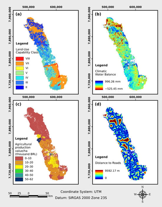
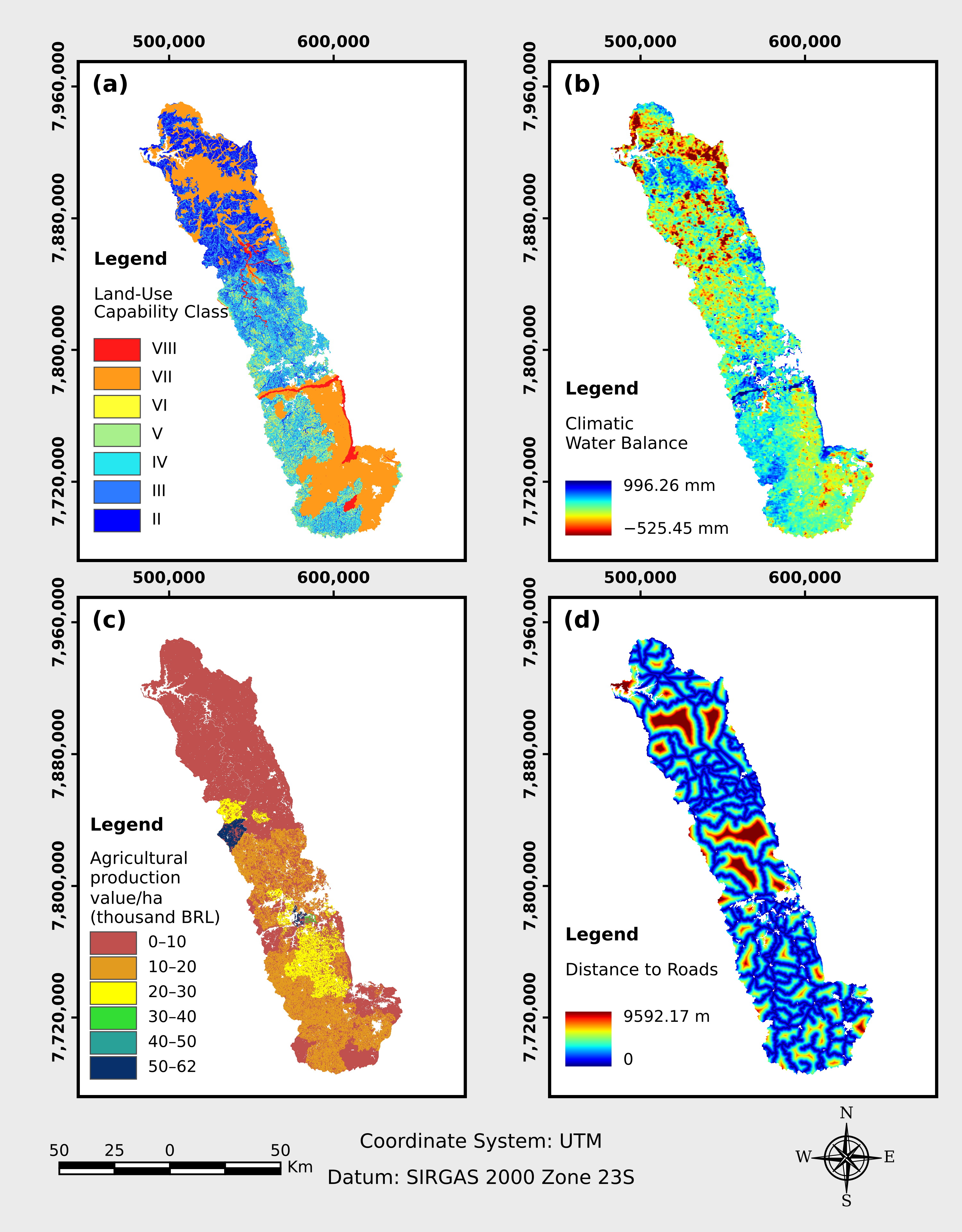
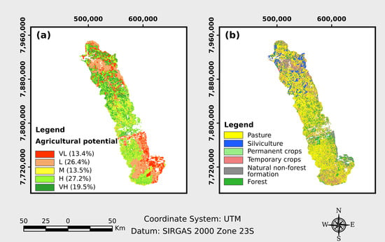
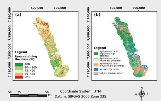

Disclaimer/Publisher’s Note: The statements, opinions and data contained in all publications are solely those of the individual author(s) and contributor(s) and not of MDPI and/or the editor(s). MDPI and/or the editor(s) disclaim responsibility for any injury to people or property resulting from any ideas, methods, instructions or products referred to in the content. |
© 2026 by the authors. Licensee MDPI, Basel, Switzerland. This article is an open access article distributed under the terms and conditions of the Creative Commons Attribution (CC BY) license.