Restorative Evaluation of Rural Waterside Landscapes in Mountainous Areas Integrating Semantic Segmentation and Machine Learning

Abstract

Rural waterfront landscapes connect ecological environments with residents’ recreational experiences, and assessing their perceived restorativeness can support improvements in rural living environments. However, complex terrain and limited data availability constrain the quantitative assessment of their visual characteristics. This study examined the Changjiang River waterfront in Jinzhai County, Anhui Province, China. Panoramic imagery, semantic segmentation, and random forest regression were integrated to derive 12 objective visual indicators of landscape composition and color characteristics and to predict four dimensions of perceived restorativeness: fascination, being away, coherence, and scope. The R² values for the hold-out test set were 0.732, 0.730, 0.722, and 0.719, respectively (n = 200). The green view index, blue view index, contrast, color count, and color complexity showed significant positive correlations with perceived restorativeness, whereas the road visibility index, mountain visual ratio, and artificial structure visibility index showed significant negative correlations. Visible blue-green elements and visual richness were associated with higher perceived-restorativeness scores, whereas images with more visually dominant road surfaces, mountains, and artificial structures tended to receive lower perceived-restorativeness scores. These findings are specific to the dry-season, low-water-level conditions observed during the November survey and should not be generalized to other seasons or hydrological conditions.

1. Introduction

With the advancement of China’s Rural Revitalization and Healthy China strategies, rural spatial development is gradually shifting from conventional functional improvement toward enhanced ecological quality and greater health benefits [1]. In this context, rural public spaces are expected not only to fulfill ecological and recreational functions but also to provide residents and other users with environmental conditions conducive to relieving everyday stress and restoring directed attention. Rural waterfront landscapes connect natural environments with rural settlements and integrate natural elements such as water, vegetation, and open space, thereby offering potential settings for psychological restoration [2]. Under the current framework for building harmonious and beautiful countryside, territory-wide landscape management has imposed more refined requirements on the environmental quality of rural areas [3]. However, existing studies on rural waterfronts have largely focused on a single dimension, such as ecological restoration or landscape beautification. Integrated research that jointly considers human perceptions, ecological benefits, and health-promoting values remains limited. Given the constraints imposed by topographic variation and seasonal change in mountainous waterfront spaces, assessing the perceived restorativeness of mountainous rural waterfront landscapes and developing corresponding spatial optimization strategies are particularly important.

In recent years, rapid advances in deep learning and computer vision have accelerated the application of artificial intelligence to the automated identification and quantification of waterfront landscape elements [4]. Semantic segmentation algorithms can process large sets of real-world images to identify their constituent landscape elements and calculate quantitative indicators, such as the green view index and blue view index. They have therefore become a widely used approach for extracting objective landscape features [5]. General-purpose segmentation models such as OneFormer achieve unified image segmentation through joint multitask training, providing technical support for the batch extraction of landscape elements across entire study areas [6]. For example, a U-Net architecture with a VGG16 encoder can be used to identify waterfront vegetation and extract its features [7]. Visual indicators such as the green view index, blue view index, color diversity, and sky openness can also be derived through semantic segmentation to reveal the relationships between landscape elements and visual perception [8]. Studies using deep learning to analyze landscape imagery have further shown that vegetation, water bodies, buildings, and spatial openness are associated with waterfront landscape quality [9,10]. Compared with urban areas, rural areas lack standardized street-view data sources because of their complex terrain and road conditions. Moreover, neither vehicle-mounted image collection nor the overhead perspective of unmanned aerial vehicle imagery can accurately reproduce the pedestrian eye-level view at a height of 1.7 m. Together, these constraints limit the objective quantification of mountainous rural waterfront landscapes.

Theories of restorative environments suggest that natural environments can improve psychological well-being by restoring directed attention and alleviating stress responses. Among these theories, Attention Restoration Theory (ART) and Stress Recovery Theory (SRT) provide the theoretical foundations for research on landscape restorativeness [11]. Within this framework, the shortened 11-item Perceived Restorativeness Scale (PRS-11) has been used to assess the perceived restorativeness of landscape spaces. It provides a useful tool for quantifying the relationship between environmental characteristics and psychological restoration. Visual elements constitute the primary source of information through which the public perceives landscapes, making perception-based evaluations important for landscape design [12]. Traditional landscape evaluation has largely relied on manual rating methods, including Scenic Beauty Estimation (SBE), the Semantic Differential method (SD), and the Analytic Hierarchy Process (AHP). These methods generally focus on indicators such as aesthetic quality, comfort, and perceived safety [13,14]. Landscape features such as vegetation, water, sky visibility, and cultural elements can all influence the perceived quality of waterfront spaces. Vegetation can enhance perceptions of naturalness and safety, whereas an excessively high proportion of water may reduce the overall quality of the experience [15,16,17]. However, existing studies have primarily focused on urban waterfronts and streetscapes, with limited attention given to the psychological restorative effects of mountainous rural waterfront landscapes. In particular, quantitative research integrating a realistic pedestrian eye-level perspective, multidimensional visual indicators, and machine-learning models remains scarce.

Meanwhile, machine-learning methods have increasingly been applied to coupled analyses linking objective landscape indicators with subjective perceptual evaluations [18]. These methods have demonstrated strong capabilities in fitting nonlinear relationships and generating predictions. Previous studies have shown that combinations of landscape elements can significantly influence visual evaluation results and that machine-learning models can effectively identify the key contributing factors. For example, naturalness, landscape richness, the green view index, and color richness positively influenced the scenic beauty of wetland parks surrounding Chaohu Lake, whereas the proportions of buildings and visible water had negative effects [19]. In addition, models such as random forest and extreme learning machine have been used to predict waterfront landscape quality. The results indicated that natural elements, including the green view index, had positive effects, confirming the applicability of machine-learning methods to landscape perception assessment [18,20]. Overall, machine-learning models can effectively explain the combined effects of landscape elements on subjective perceptions and thus provide a reliable technical approach. However, existing coupled modeling studies have primarily focused on urban waterfronts and wetland parks. Nonlinear coupling research that accounts for the distinctive topography of mountainous rural areas and is tailored to human-centered perceptions of restorativeness remains underdeveloped. Further research is therefore required to improve restorative assessments and design practices for rural waterfront spaces.

Although machine learning and image analysis have been applied to landscape perception assessment, three important gaps remain. First, most studies have focused on overall visual quality and aesthetic preference in urban waterfronts, streetscapes, or wetland parks. Few have disaggregated perceived restorativeness into fascination, being away, coherence, and scope, making it difficult to compare how the same visual feature is associated with different psychological dimensions. Second, existing studies have largely relied on standardized street-view imagery, online images, or overhead imagery. Relatively few have characterized the environment actually visible from a pedestrian eye-level perspective along a continuous river reach or adequately distinguished physical proximity to the waterfront from the visual visibility of the water surface. Third, image-level perception predictions have rarely been translated into segment-based spatial diagnoses of continuous waterfront corridors, limiting the connection between quantitative results and site-specific renewal decisions.

Accordingly, this study hypothesizes that perceived restorativeness in rural waterfront landscapes is statistically associated with objective physical elements and color characteristics and that the predictive contributions of visual indicators may differ across the four dimensions. This study does not seek to develop new semantic segmentation or machine-learning algorithms. Instead, it constructs and evaluates a pedestrian-scale assessment and spatial diagnostic workflow for continuous waterfront corridors in mountainous rural areas. Specifically, it addresses three questions: (1) How are visible landscape elements and color characteristics distributed along the study reach? (2) To what extent can these indicators predict the four dimensions of perceived restorativeness? (3) How can variations in scores along the river provide a preliminary basis for section-specific renewal? The workflow uses panoramic images captured at a pedestrian eye level of 1.7 m to represent the environment actually visible to pedestrians, links seven categories of landscape elements and five color features to the four PRS-11 dimensions, and maps the image-level assessment results onto the continuous waterfront corridor. Its transferable contribution lies in the evaluation logic and spatial diagnostic workflow rather than in the model parameters or scoring thresholds derived from a single study area.

2. Materials and Methods

2.1. Study Area and Data

2.1.1. Study Area and Research Setting

Mountainous rural waterfront spaces provide an important spatial interface between natural ecosystems and the living environments of rural residents. Under the combined influence of topography, hydrological processes, and human activities, these landscapes typically exhibit a complex pattern in which mountains, water bodies, forests, farmland, and villages are closely interwoven [21]. Compared with rural landscapes in plains, mountainous rural landscapes are more strongly shaped by elevation, slope, hydrological networks, and construction activities, resulting in highly heterogeneous spatial patterns [22]. Different combinations of natural and built landscape elements can also create distinct visual characteristics and subsequently influence public landscape perceptions and evaluations, making mountainous rural waterfronts important subjects for landscape perception research [23].

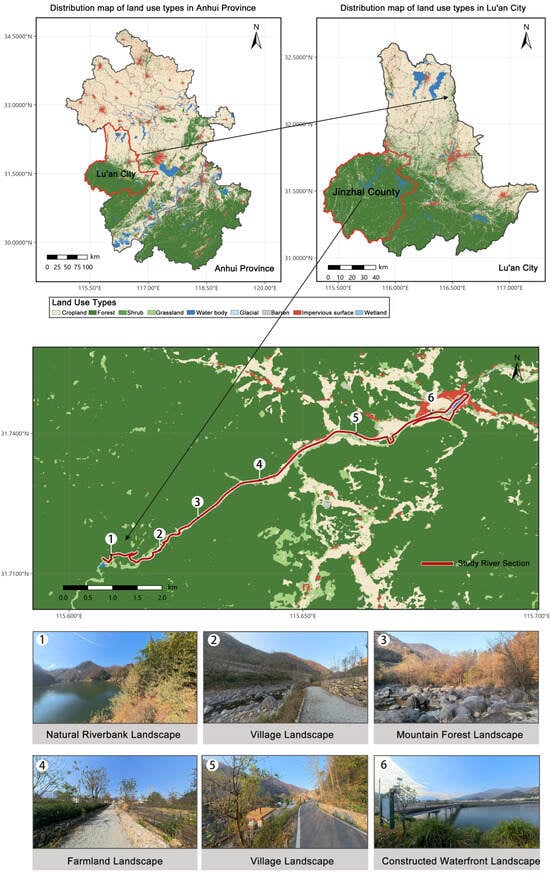
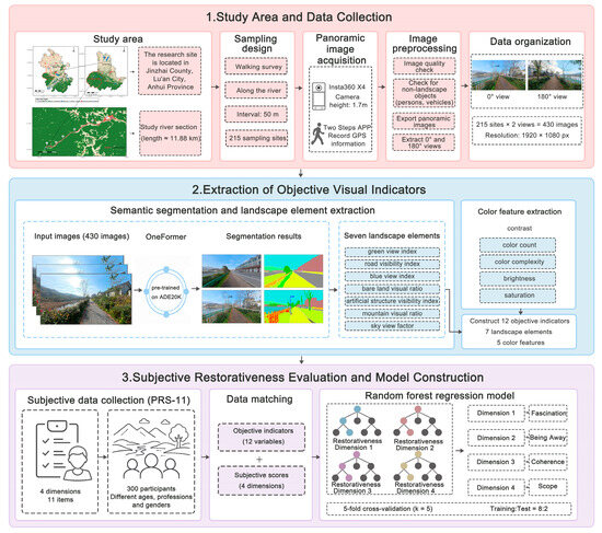
Based on the characteristic features of mountainous rural waterfront landscapes, this study selected a representative reach of the Changjiang River in Jinzhai County, Anhui Province, China, as the study area. Jinzhai County is located in the Dabie Mountains and is characterized by prominent mountainous terrain, with natural environments, agricultural production, and village life closely interwoven across its rural areas. In recent years, the county has continuously implemented rural landscape character management and human settlement improvement initiatives under the framework for building harmonious and beautiful countryside, making it representative of the wider region. As a National Rural Revitalization Demonstration County, Jinzhai has also systematically explored approaches to rural landscape character management [3]. Based on previous research and field surveys, the river reach extending from the Changjiang River Reservoir Scenic Area to Xiayejialou was ultimately selected as the study site (Figure 1). The study reach has a total shoreline length of approximately 11.88 km.

Figure 1. Location map of the study area.

The river reach is characterized by a relatively well-preserved natural environment and connects a variety of landscape types, including farmland, villages, mountain forests, and natural riverbanks. Owing to differences in topographic conditions, land-use patterns, and the intensity of built development, landscape composition and spatial form vary considerably among the river sections. This diversity provides a range of samples for analyzing the relationship between visual landscape elements and perceived restorativeness. Overall, the study reach exhibits representative characteristics of mountainous rural waterfront landscapes and provides a useful case for their restorative assessment and spatial optimization.

The study reach includes natural riverbanks, village roads, and public activity nodes, allowing varying levels of human intervention to occur within the same continuous waterfront corridor. This site configuration facilitates comparisons among different combinations of visible blue-green elements and hardscape surfaces. However, the findings should be generalized with caution and are most applicable to waterfront spaces with comparable terrain, seasonal conditions, and patterns of use. The value of this case lies primarily in revealing the relationships among topographic constraints, landscape composition, and pedestrian-visible environments. It also provides an assessment workflow for continuous river corridors rather than assuming that a single study area can represent all mountainous rural waterfront environments.

2.1.2. Data Collection and Processing

Data were collected through a combination of field surveys and panoramic image acquisition [12]. Image collection was conducted under clear and haze-free weather conditions with mild temperatures [24,25]. Images were collected on 13 and 14 November 2025, from 09:00 to 12:00 and from 14:00 to 17:00. One researcher walked along all riverside roads of the Changjiang River and captured images using an Insta360 X4 panoramic camera (Arashi Vision Inc., Shenzhen, China). The camera was positioned at approximately 1.7 m above the ground [26]. Another researcher simultaneously recorded the geographic coordinates of each sampling point using the Two Steps APP (v8.0.6) on a smartphone. The sampling interval was approximately 50 m. Panoramic images were collected at 215 sampling points located along the road centerlines. Efforts were made to exclude non-landscape elements, such as pedestrians and moving vehicles, from the images. The panoramic images were processed using Insta360 Studio [12]. After export, the panoramic images were subjected only to view extraction and resolution standardization; no manual adjustments were made to brightness, contrast, saturation, hue, gamma, white balance, or color balance. All images met the required clarity standard. Using the direction of travel as 0°, two views at 0° and 180° were extracted from each panoramic image in flat-view mode, yielding a total of 430 images [27]. These images represented the forward and backward views along the riverside walking route and captured the surrounding environment at each sampling point. This standardized selection was intended to reflect the principal viewing directions during movement rather than deliberately maximize water visibility. All images were standardized to a resolution of 1920 × 1080 pixels and matched with the corresponding GPS information in ArcMap 10.8. The spatial data were referenced to the China Geodetic Coordinate System 2000 (CGCS2000; EPSG:4490).

2.2. Research Framework

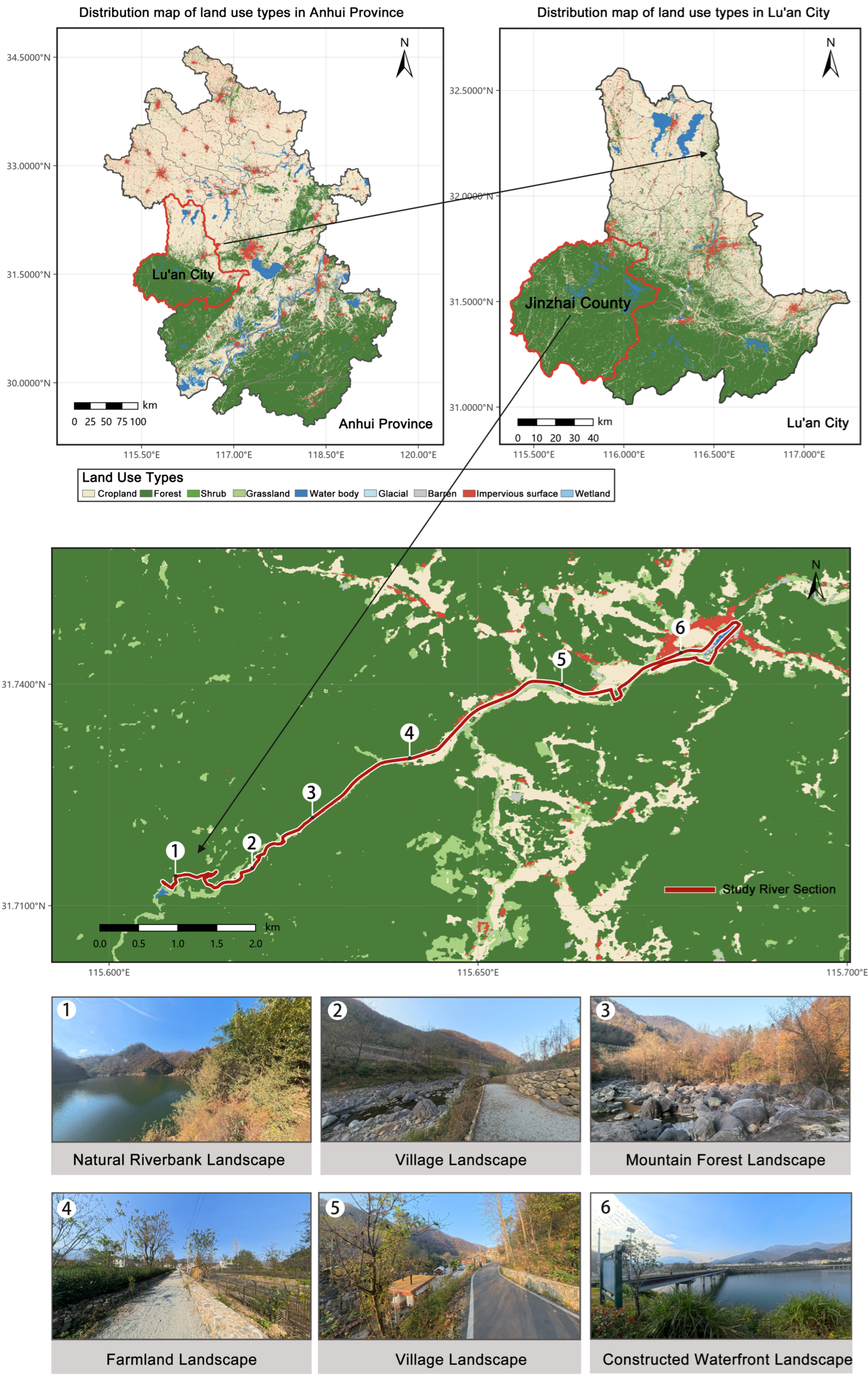
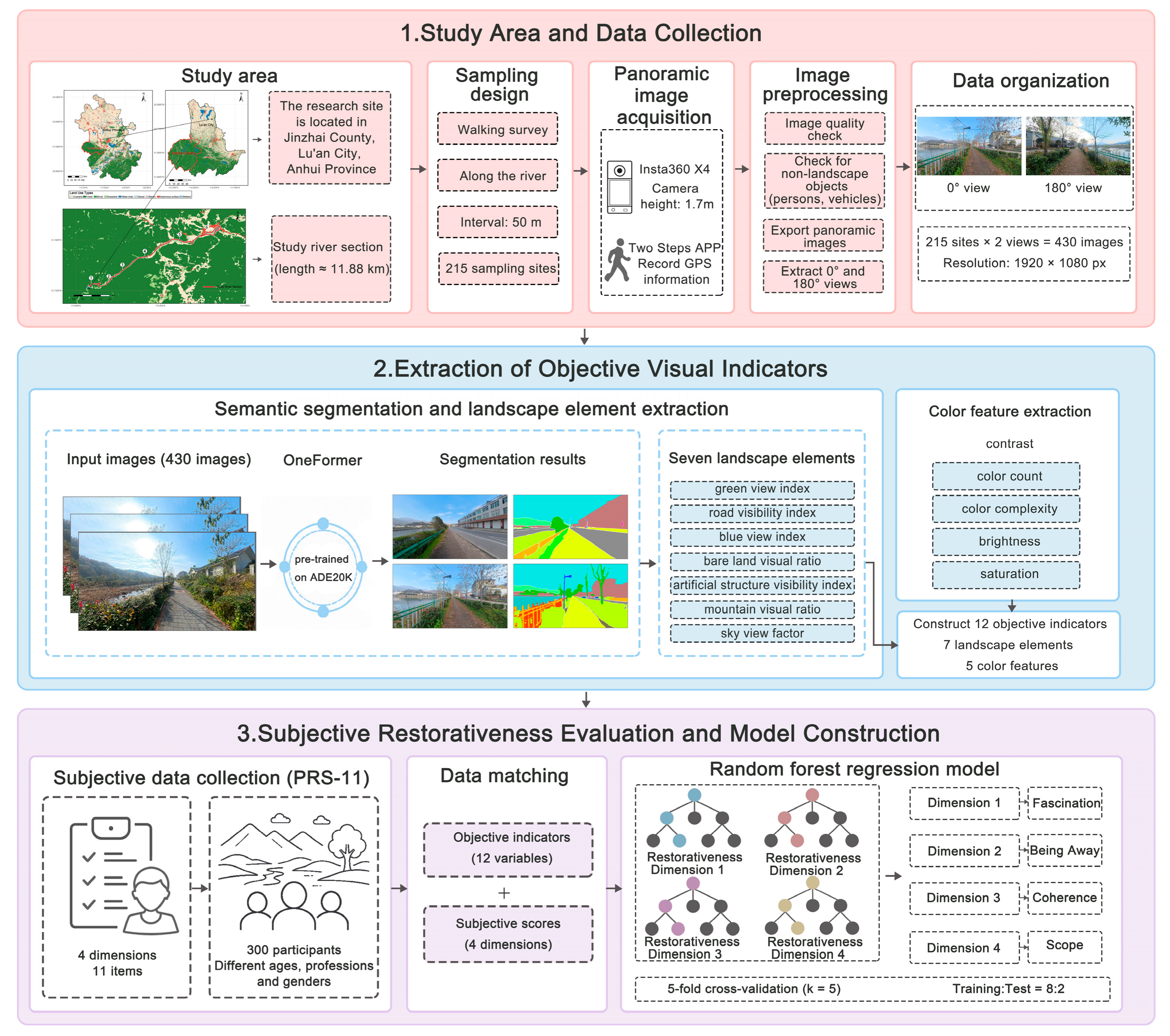
Building on previous studies, this study integrates panoramic imagery, deep learning, and machine-learning methods to develop a framework for assessing the perceived restorativeness of rural waterfront landscapes. The framework comprises four stages: data collection and processing, objective indicator quantification, subjective perception assessment, and results analysis and application (Figure 2). First, waterfront landscape images were obtained through field-based panoramic photography. Second, objective visual landscape indicators were extracted, and perceived restorativeness data were collected using the PRS-11. Finally, a random forest model was used to examine the predictive associations between landscape elements and perceived restorativeness.

Figure 2. Research framework diagram.

2.3. Landscape Feature Extraction Using Deep Learning

2.3.1. Semantic Segmentation and Landscape Element Extraction

The OneFormer model pretrained on the ADE20K dataset [28] was used for semantic image segmentation. ADE20K is a scene-understanding dataset released by MIT in 2016 and contains 150 semantic categories. Compared with conventional CNN-based semantic segmentation models, OneFormer unifies multiple image segmentation tasks within a single framework and offers advantages in recognizing complex scenes [6]. It is therefore suitable for extracting diverse landscape elements from rural waterfront images. Considering the characteristics of rural waterfront environments and drawing on previous studies, seven landscape-element categories were selected [29]: sky [30], water bodies [31], vegetation [32], road surfaces [31], mountains [33], built structures [31], and bare land [34]. The proportion of each category within each image was then calculated.

The seven categories represent natural backgrounds, water and shoreline resources, and interfaces shaped by human activities, allowing the visible composition of different scenes to be compared. Notably, a low blue view Index may result from the contraction of the water surface during the dry season. It may also be influenced by road orientation, riverbank slopes, and visual obstruction from vegetation. In this study, “artificial structures” comprise buildings, walls, fences, and bridges, which were merged into a single category to calculate the artificial structure visibility index.

Pixels assigned to other ADE20K classes were retained in the total pixel count but were not included in the seven landscape-element categories or used as variables in subsequent analyses. Therefore, the proportions of the seven categories were not renormalized to sum to 100%. The mean proportions of the seven categories in Table 1 sum to 92.94%, while the remaining 7.06% represents pixels assigned to other classes.

Table 1. Descriptive statistics of the objective visual indicators.

Indicator	Maximum	Minimum	Mean	Median	Standard Deviation	Standard Error	Coefficient of Variation
road visibility index	40.23	0.00	14.11	17.59	10.47	0.50	0.74
sky view factor	42.28	3.13	26.95	27.79	8.64	0.42	0.32
green view index	67.61	0.00	16.95	14.68	12.35	0.60	0.73
artificial structure visibility index	39.19	0.00	6.24	4.54	6.12	0.30	0.98
mountain visual ratio	67.45	0.00	14.52	7.91	14.68	0.71	1.01
blue view index	29.66	0.00	2.04	0.00	5.11	0.25	2.50
bare land visual ratio	67.96	0.00	12.13	8.19	12.84	0.62	1.06
brightness	153.74	101.27	129.24	129.45	9.06	0.44	0.07
contrast	77.80	37.87	58.86	58.11	6.79	0.33	0.12
saturation	37.87	6.48	17.38	17.76	5.56	0.27	0.32
color count	1671	311	894.3	877.5	250.87	12.10	0.28
color complexity	7.91	6.96	7.57	7.57	0.16	0.01	0.02

Following automatic segmentation, all 430 segmentation results were manually inspected by comparing the original images with the corresponding segmentation maps. The inspection focused on the spatial extent, class assignment, and boundary delineation of mountains, vegetation, bare land, and road surfaces. It covered different scenes in the upstream, midstream, and downstream sections. The identified extents of the major elements were generally consistent with those in the original images. Overall, the qualitative inspection showed that the segmentation results were generally consistent with the original images, and no recurring class-specific misclassification patterns that would systematically affect the corresponding visibility indicators were identified. This procedure constituted qualitative quality control. Because no manually annotated pixel-level ground-truth masks were created, intersection over union (IoU) and F1 scores were not calculated.

The pixel proportions of the seven semantic categories were used to derive seven landscape-composition indicators: the road visibility index, sky view factor, green view index, artificial structure visibility index, mountain visual ratio, blue view index, and bare land visual ratio. The sky view factor was calculated as the proportion of sky pixels relative to the total number of pixels in an image. Together, the seven semantic-segmentation-derived indicators and five color indicators—brightness, contrast, saturation, color count, and color complexity—formed the 12 objective visual indicators used in this study.

Following the semantic-category pixel-proportion method adopted in previous visual perception research [12], the green view index (GVI) was calculated from pixels classified as vegetation, while the blue view index (BVI) was calculated using the same method for pixels classified as water:

$$\begin{array}{c}\mathit{GVI} ={\displaystyle \frac{N_{\mathit{vegetation}}}{N_{\mathit{total}}}}\times 100\% \end{array}$$

(1)

$$\begin{array}{c}\mathit{BVI}={\displaystyle \frac{N_{\mathit{water}}}{N_{\mathit{total}}}}\times 100\%\end{array}$$

(2)

where N_vegetation and N_water denote the numbers of pixels classified as vegetation and water, respectively, and N_total denotes the total number of pixels in the corresponding image.

2.3.2. Color Feature Extraction

The OpenCV (v4.12.0) and Pillow (v12.0.0) libraries in Python 3.10 were used to calculate the color indicators in batches. Five color features were extracted from each image: brightness, contrast, saturation, color count, and color complexity [35]. These indicators were calculated using the equations presented below.

Mean brightness was calculated as follows [36]:

$$\begin{array}{c}B={\displaystyle \frac{1}{N}}{\displaystyle \sum _{i=1}^N}\mathit{brightness}\left(p_i\right)\end{array}$$

(3)

where B is the average brightness, N is the total number of pixels in the image, and brightness(pi) is the brightness of the i-th pixel, calculated as the mean of its RGB channel values.

Contrast was calculated as follows [36]:

$$\begin{array}{c}C=\sqrt{{\displaystyle \frac{1}{N}}{\displaystyle \sum _{i=1}^N}{(p_i-\overline{p})}^2}\end{array}$$

(4)

where C is the contrast, p_i is the brightness of the i-th pixel, and $\overline{p}$ is the mean brightness of all pixels.

Saturation was calculated as follows [37]:

$$\begin{array}{c}S={\displaystyle \frac{1}{N}}{\displaystyle \sum _{i=1}^N}\mathit{saturation}\left(p_i\right)\end{array}$$

(5)

where S is the average saturation, p_i is the saturation level of the i-th pixel, calculated using the HSV color model, and N is the total number of pixels in the image.

The number of colors was calculated as follows [38]:

$$\begin{array}{c}M=\mid \left\{\right(R_i,G_i,B_i)\mid i=1, 2, \dots , N\}\mid \end{array}$$

(6)

where M represents the total number of distinct colors in the image, (R_i,G_i,B_i) denotes the RGB value of the i-th pixel, and N is the total number of pixels in the image.

The color complexity can be represented as [39]:

$$\begin{array}{c}E=-{\displaystyle \sum _{i=1}^M}p\left(c_i\right){\mathit{log}}_{2}p\left(c_i\right)\end{array}$$

(7)

where E is the color entropy, c_i are the distinct colors, p(c_i) is the proportion of pixels of color c_i, and M is the number of distinct colors.

2.4. Restorativeness Assessment Using Explainable Machine Learning

2.4.1. Collection of Subjective Perceived Restorativeness Data

At the subjective level, attention restoration theory (ART) proposes that natural environments facilitate the restoration of cognitive resources by engaging involuntary attention. The Perceived Restorativeness Scale (PRS) was developed based on ART and has demonstrated good psychometric reliability [40]. To assess public perceptions of landscape restorativeness, this study adopted the shortened Perceived Restorativeness Scale (PRS-11) developed by Pasini et al. [41]. Compared with the original 26-item PRS (PRS-26), the PRS-11 improves administration efficiency by reducing the number of items while retaining sound psychometric properties. The scale comprises 11 items across four core dimensions: fascination, being away, coherence, and scope. Evidence from its original development and validation provided the basis for selecting this scale. The present study retained this four-dimensional framework, collected ratings using a five-point Likert scale, and examined internal consistency, inter-rater agreement, and discriminant validity using the survey data.

Of the 430 images, 200 were selected for the subjective perception assessment. These 200 images were randomly assigned without duplication to 10 questionnaire versions, with 20 images in each version. Here, random assignment refers only to the allocation of images across questionnaire versions and does not indicate that the 200 images were randomly sampled from the full set of 430 images. A total of 300 adult respondents completed the questionnaire, including 158 men and 142 women from diverse age and occupational groups. Each of the 10 versions was completed by 30 respondents, and each respondent evaluated only the 20 images included in their assigned version. Consequently, each image received 30 independent valid ratings, yielding 6000 respondent–image records. The questionnaire was administered online through Wenjuanxing. Images were presented in random order within each version. No overall completion-time limit or fixed image-viewing duration was imposed; respondents were permitted to return to and revise their responses, and no restrictions were placed on the type of device used. Most respondents completed the questionnaire using smartphones. For each respondent–image record, the arithmetic mean of the items corresponding to each of the four dimensions was first calculated. The dimension scores provided by the 30 respondents evaluating the same image were then averaged to obtain the four image-level perceived-restorativeness scores, which were used as the dependent variables in subsequent analyses.

2.4.2. Reliability and Discriminant Validity of Subjective Ratings

Based on the 6000 respondent–image rating records, Cronbach’s α was used to assess the internal consistency of each dimension. The Spearman–Brown coefficient was additionally calculated for scope, which comprised only two items. Because the 20 images in each questionnaire version were evaluated by the same group of 30 respondents, a two-way random-effects, absolute-agreement, average-measures ICC(2,30) was calculated separately for each version, and the median and range across versions were reported. Discriminant validity was assessed using the heterotrait–monotrait ratio (HTMT), primarily based on the item means for the 200 images, with results based on the 6000 rating records included as a supplementary analysis. In addition, the associations between demographic characteristics and image ratings were examined using linear models that included image fixed effects and respondent gender, age, educational attainment, and disciplinary background.

There were no missing data for any PRS-11 item. Cronbach’s α values for fascination, being away, and coherence were 0.894, 0.891, and 0.873, respectively. For scope, Cronbach’s α and the Spearman–Brown coefficient were 0.841 and 0.842, respectively. Cronbach’s α for the full 11-item scale was 0.952. The median ICC(2,30) values for the four dimensions were 0.710, 0.703, 0.587, and 0.471, with corresponding ranges of 0.461–0.926, 0.076–0.912, 0.220–0.854, and 0.090–0.763, respectively. These results indicate that the reliability of the aggregated ratings varied across questionnaire versions. The correlations between the image ratings before and after demographic adjustment ranged from 0.998 to 0.999, and the mean absolute changes were only 0.012–0.013 points, indicating that adjustment for the observed demographic characteristics produced only minor changes.

At the respondent–image record level, the HTMT values for fascination–being away, fascination–coherence, and being away–coherence were 0.970, 0.919, and 0.917, respectively. At the image level, the corresponding values were 0.995, 0.966, and 0.964, indicating limited discriminant validity among the first three dimensions. The HTMT values between scope and the other dimensions ranged from 0.746 to 0.827 at the record level and from 0.725 to 0.817 at the image level, indicating comparatively stronger discriminant validity. Therefore, this study retained the established four-dimensional structure of the PRS-11 but interpreted differences among the first three dimensions cautiously. Because no common anchor images were included across questionnaire versions, unobserved differences between respondent groups could not be fully excluded.

The four restorative dimensions were modeled separately as individual dependent variables; therefore, their high intercorrelations did not create multicollinearity among the predictors within any individual model. To preserve the theoretical structure of the PRS-11 and comparability with previous studies, the factor structure was not redefined through exploratory analysis. The composite score was used as the primary output for spatial analysis, while differences among the first three dimensions were interpreted cautiously.

2.4.3. Development of an Explainable Random Forest Prediction Model

Random Forest constructs multiple decision trees from bootstrap-resampled training samples, while the degree of feature subsampling is controlled by the max_features parameter [42,43]. The algorithm can model nonlinear relationships and estimate variable importance, but its predictive performance must still be evaluated using independent test data and cross-validation [43,44,45]. Therefore, this study used Random Forest regression to analyze the objective and subjective data described above [46]. A nonlinear mapping model was developed between objective landscape elements and subjective psychological perceptions.

The four dimensions of perceived restorativeness were specified as dependent variables. These dimensions were fascination, being away, coherence, and scope. Subjective scores were derived from 300 valid questionnaires covering 200 images. The resulting image-level records formed the modeling sample for Random Forest regression (n = 200).

The composite perceived-restorativeness score for each image was calculated as the equally weighted arithmetic mean of the scores for fascination, being away, coherence, and scope. The composite scores for the 0° and 180° views at the same sampling point were then averaged, yielding composite perceived-restorativeness scores for 215 sampling points. Observed image-level scores were used for the 200 questionnaire-rated images, whereas model-predicted values were used for the remaining 230 images. The latter were generated by models fitted using all 200 rated images and therefore represent full-sample model predictions rather than out-of-fold predictions. To visualize the spatial variation in perceived restorativeness across the study area, the composite scores for the sampling points were imported into ArcGIS 10.8.

A fixed image-level hold-out split was first created using an 80:20 ratio, comprising 160 training images and 40 images in the hold-out test set, with a random seed of 42. This split was used to fit the models and report the training-set and hold-out test set results. All four models used the same predefined configuration. Each forest comprised 100 regression trees and used the squared-error criterion. Tree depth was unrestricted; at least two samples were required to split an internal node, at least one sample was required in a terminal leaf, and all predictor variables were considered at each split. Bootstrap sampling was enabled, each bootstrap sample contained the same number of observations as the corresponding training set, and out-of-bag estimation was not used. A random seed of 42 was applied, and model fitting used all available processing cores. No data-driven hyperparameter tuning was performed, and the hold-out test set was not used for model selection.

Separately, five-fold cross-validation (k = 5) was conducted to characterize the variation in model performance across data partitions [45]. In the standard image-level analysis, all 200 rated images were randomly shuffled using a fixed seed of 42 and divided into five folds. In each iteration, four folds comprising 160 images were used for training, and the remaining fold comprising 40 images was used for validation. A focused sampling-point-grouped analysis was also conducted, in which the 0° and 180° views from the same sampling point were assigned to the same fold. The same predefined Random Forest configuration was used in every fold. The mean and standard deviation across the five validation folds are reported in Table 2. Thus, the five-fold cross-validation results are reported separately from the hold-out results. Model performance was evaluated using the coefficient of determination (R²), root mean square error (RMSE), and mean absolute error (MAE) [47]. Before interpreting variable importance, multicollinearity among the 12 predictors was assessed using variance inflation factors (VIFs), with each predictor regressed on the remaining predictors. A focused VIF assessment was also conducted separately for the green view index, blue view index, and road visibility index. Variable importance analysis was used to interpret model predictions [48].

Table 2. Five-fold cross-validation results under image-level and sampling-point-grouped data partitioning (mean ± SD across five validation folds).

Dimension	Cross-Validation Method	R2	RMSE	MAE
Fascination	Image-level	0.4783 ± 0.2025	0.2751 ± 0.0537	0.2117 ± 0.0421
	Sampling-point-grouped	0.5432 ± 0.0833	0.2624 ± 0.0258	0.2015 ± 0.0136
Being away	Image-level	0.5159 ± 0.1810	0.2423 ± 0.0445	0.1858 ± 0.0304
	Sampling-point-grouped	0.5623 ± 0.0852	0.2347 ± 0.0248	0.1823 ± 0.0182
Coherence	Image-level	0.4840 ± 0.2126	0.1995 ± 0.0333	0.1511 ± 0.0268
	Sampling-point-grouped	0.5218 ± 0.0870	0.1986 ± 0.0202	0.1545 ± 0.0128
Scope	Image-level	0.4279 ± 0.1739	0.1878 ± 0.0294	0.1431 ± 0.0239
	Sampling-point-grouped	0.5109 ± 0.1076	0.1782 ± 0.0195	0.1377 ± 0.0076

To examine spatial transfer within the study corridor, leave-one-section-out validation was also conducted using the upstream, midstream, and downstream sections as spatial blocks, comprising 78, 62, and 60 rated images, respectively. In each of three iterations, the models were trained on two sections and evaluated on the remaining section using the same predictors and random-forest configuration. Section-specific and pooled R², RMSE, and MAE were calculated.

Pearson correlation analysis was further conducted to quantify the associations between the visual indicators and perceived restorativeness. The analysis was based on the 200 rated images, with each visual indicator paired with the observed mean score for the corresponding dimension of perceived restorativeness; model-predicted scores were not used. Pearson correlation coefficients (r) were calculated using Python, with α = 0.05 as the significance level. Correlations were considered statistically significant only when p < 0.05.

3. Results

3.1. Results of Objective Indicator Extraction

A semantic segmentation model was used to identify landscape elements in the panoramic images, and the statistical distributions of the indicators were analyzed. The 12 indicators were measured on different scales (Table 1). The seven landscape-composition indicators were expressed as the percentage of pixels assigned to each corresponding category relative to the total number of pixels in the image. Brightness, contrast, and saturation were statistics calculated from image pixels. Color count represented the number of distinct RGB color combinations occurring in an image, while color complexity was expressed as color entropy. Therefore, the absolute values of different indicator types should not be compared directly. The interpretation primarily considered the mean, median, and coefficient of variation of each indicator.

The results showed that the landscape composition of the study area was dominated by natural elements. The sky view factor had the highest mean proportion (26.95%), with a coefficient of variation (CV) of 0.32. The green view index had a mean of 16.95% and a CV of 0.73, indicating marked spatial variation in vegetation visibility. The mountain visual ratio and road visibility index averaged 14.52% and 14.11%, respectively, together constituting the main visual interfaces of the waterfront space. The mountain visual ratio had a CV of 1.01, indicating substantial differences in mountain visibility among sampling points. The bare land visual ratio averaged 12.13%, with a CV of 1.06, indicating a relatively dispersed spatial distribution. The artificial structure visibility index averaged 6.24%. Although its overall proportion was relatively low, its CV was high (0.98), with higher values concentrated in village areas and at road nodes. The blue view index had the lowest mean (2.04%) but the highest CV (2.50), indicating low overall water visibility and pronounced spatial variation among sampling points.

As shown by the median values in Table 1, the blue view index had a median of 0 and a mean of 2.04%. This indicates that the water surface was not directly visible in many views, whereas a small number of views contained relatively high proportions of visible water, resulting in the high CV.

Regarding the color features, the CVs of brightness, contrast, and color complexity were 0.07, 0.12, and 0.02, respectively, indicating relatively limited variation within the image sample. Saturation had a mean of 17.38 and a CV of 0.32, while color count had a mean of 894.30 and a CV of 0.28; both exhibited more pronounced relative variation among images. The mean and median of color complexity were both 7.57, indicating a relatively concentrated distribution.

All results reported in this section correspond to the dry-season and low-water-level survey conditions of November 2025. Overall, the visual environment of the study area was dominated by natural landscape elements. Spatial differences were most evident in vegetation, water visibility, and topographic conditions, whereas the color indicators were comparatively stable overall.

3.2. Evaluation of Model Predictive Performance

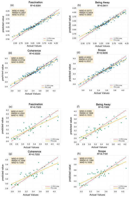
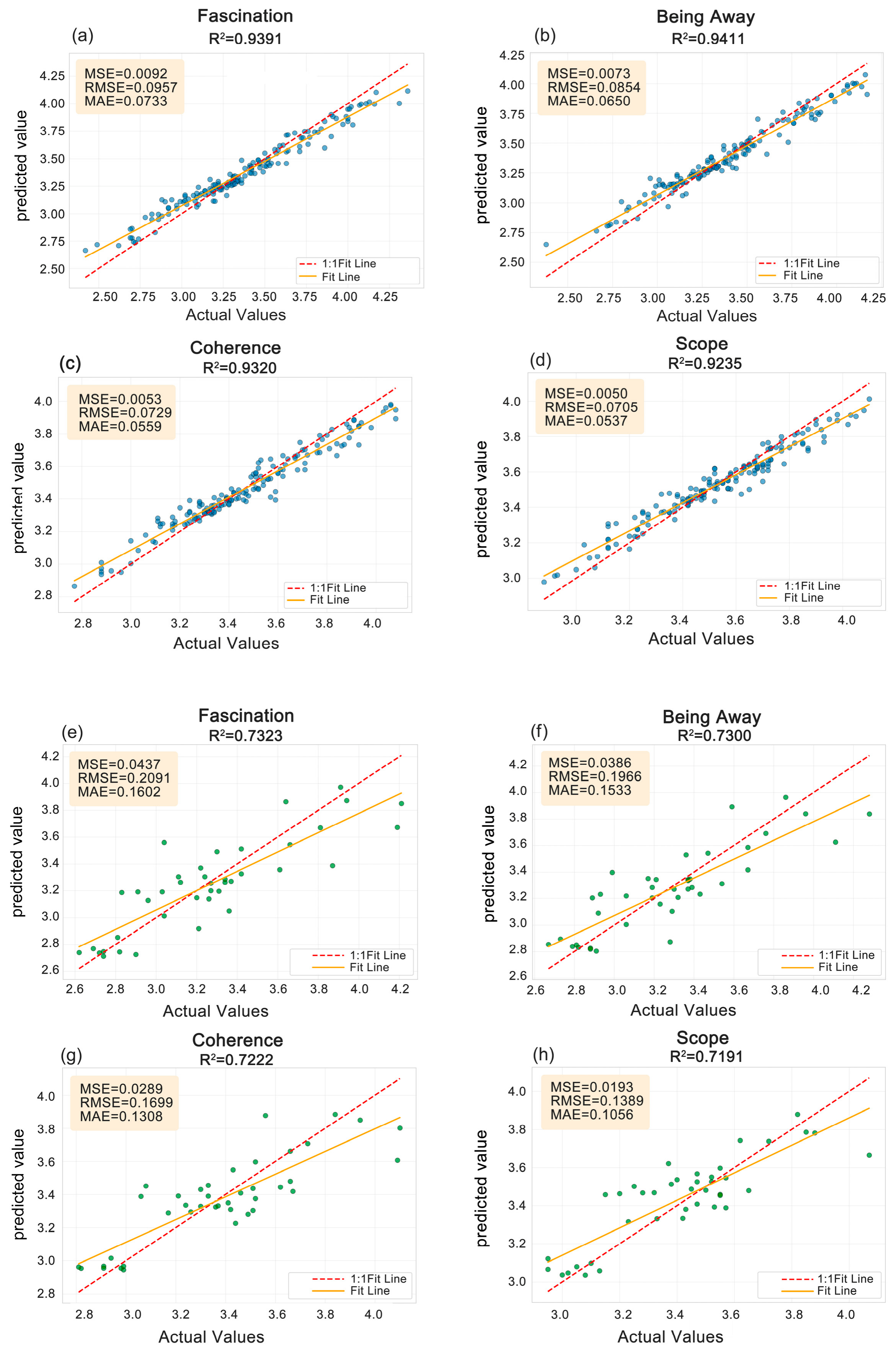
Figure 3 presents the results of the hold-out evaluation. Across the four models, the R² values ranged from 0.924 to 0.941 on the training set and from 0.719 to 0.732 on the hold-out test set. Specifically, the R² values for the hold-out test set were 0.732, 0.730, 0.722, and 0.719 for fascination, being away, coherence, and scope, respectively. These results describe the models’ predictive performance under the fixed hold-out evaluation. The five-fold cross-validation results are reported separately in Table 2.

Figure 3. Random Forest performance: (a–d) training set (blue dots); (e–h) hold-out test set (green dots).

Under standard image-level five-fold cross-validation, the mean R² values ranged from 0.4279 to 0.5159. Under sampling-point-grouped five-fold cross-validation, in which the two views from the same sampling point were retained in the same fold, the mean R² values ranged from 0.5109 to 0.5623. The grouped analysis did not reduce the mean R² and showed lower between-fold variability. Thus, this focused sensitivity check provided no indication that separating paired views materially increased the mean cross-validation performance.

Together, the hold-out evaluation and five-fold cross-validation provide complementary estimates of internal predictive performance. Leave-one-section-out validation yielded pooled R² values of 0.2174, 0.2988, 0.1685, and 0.0986 for fascination, being away, coherence, and scope, respectively (RMSE: 0.2477–0.3478; MAE: 0.1973–0.2689). For composite perceived restorativeness, the R², RMSE, and MAE were 0.2727, 0.2631, and 0.2075, respectively. Because performance varied among the held-out sections, the corridor map is interpreted as relative within-corridor variation under the present survey conditions rather than as a spatially transferable classification.

3.3. Feature Importance Analysis and Differences Across Dimensions

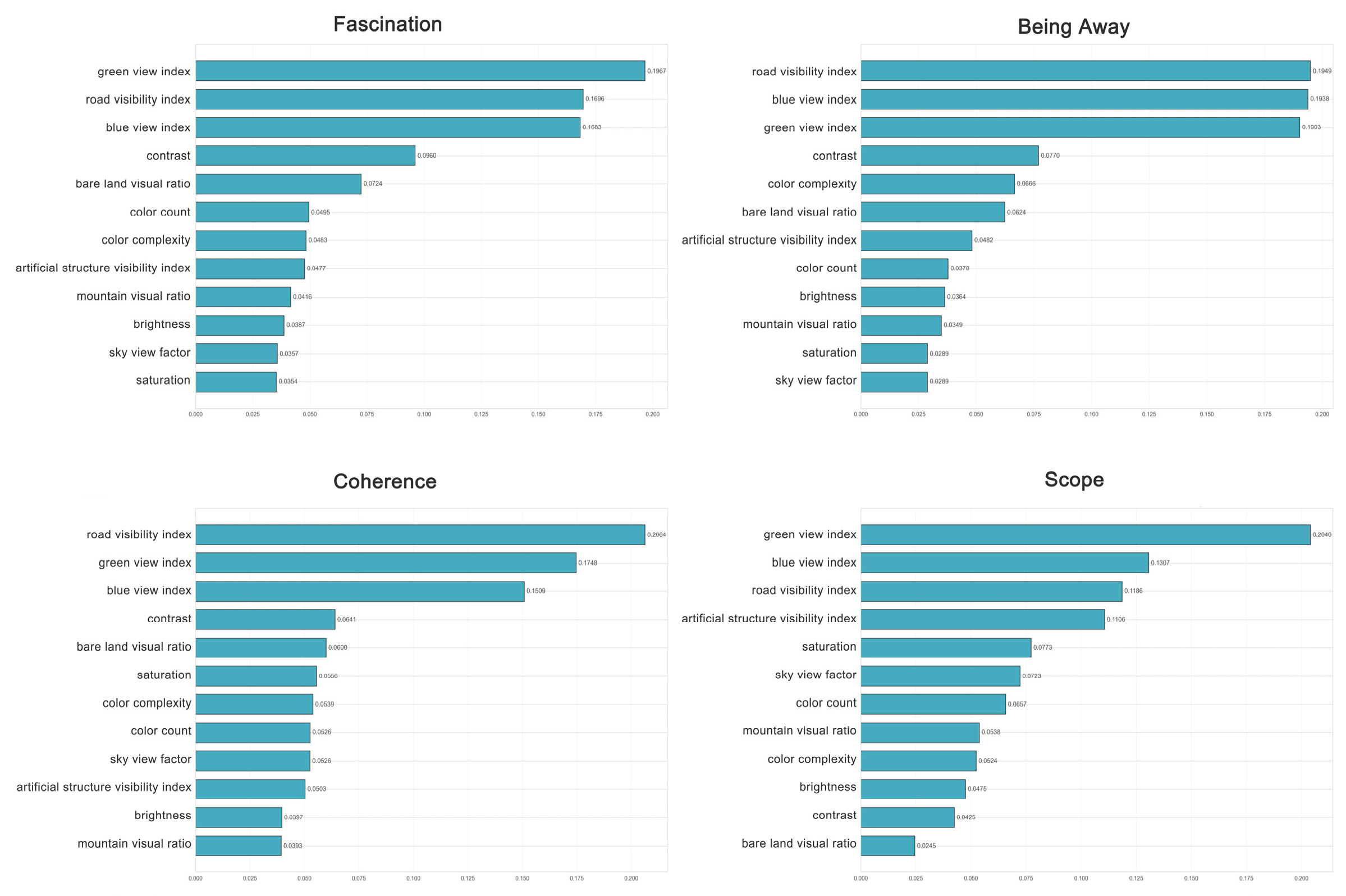
The four dimension-specific models achieved similar predictive accuracy. This indicates that, under the current validation conditions, the models performed comparably in predicting the different dimensions of perceived restorativeness. The feature importance rankings identified visual indicators with relatively high predictive contributions. Given the substantial image-level overlap among fascination, being away, and coherence, differences in predictor rankings across the four fitted models are presented as exploratory patterns rather than as evidence of clearly distinct dimension-specific predictor structures (Figure 4).

Figure 4. Feature-importance rankings for the four perceived-restorativeness dimensions.

The random forest variable importance analysis showed that the green view index, blue view index, and road visibility index made relatively high predictive contributions across multiple dimensions of perceived restorativeness. Exploratory differences in the importance rankings of the visual indicators were observed across the four fitted models.

Across the complete 12-predictor set, the VIF values ranged from 2.00 to 7.66, with the highest values observed for the sky view factor (7.66) and mountain visual ratio (7.48). The VIF values for the green view index, blue view index, and road visibility index were 5.39, 2.16, and 3.71, respectively. In the focused assessment restricted to these three predictors, the corresponding VIF values were 1.04, 1.36, and 1.36, indicating limited redundancy among them. Because moderate shared variation remained among some indicators in the complete predictor set, the rankings in Figure 4 are interpreted as relative predictive contributions within the fitted models rather than as independent effects.

3.4. Overall Landscape Restorativeness Scores and Spatial Distribution

To compare composite perceived-restorativeness levels among river sections, descriptive statistics were calculated for the scores of the 215 sampling points in the upstream, midstream, and downstream sections (Table 3). The downstream section had the highest mean score, followed by the upstream section, whereas the midstream section had a relatively lower mean score. The median scores followed the same relative order. However, the score ranges overlapped across the three sections, indicating variation among sampling points within each section. Therefore, the overall trend of a river section should not be equated with the restorativeness level of every sampling point within that section.

Table 3. Descriptive statistics of composite perceived-restorativeness scores across the upstream, midstream, and downstream sections.

River Section	Number of Points	Mean ± SD	Median
Upstream	72	3.37 ± 0.27	3.42
Midstream	61	3.29 ± 0.16	3.29
Downstream	82	3.49 ± 0.24	3.47

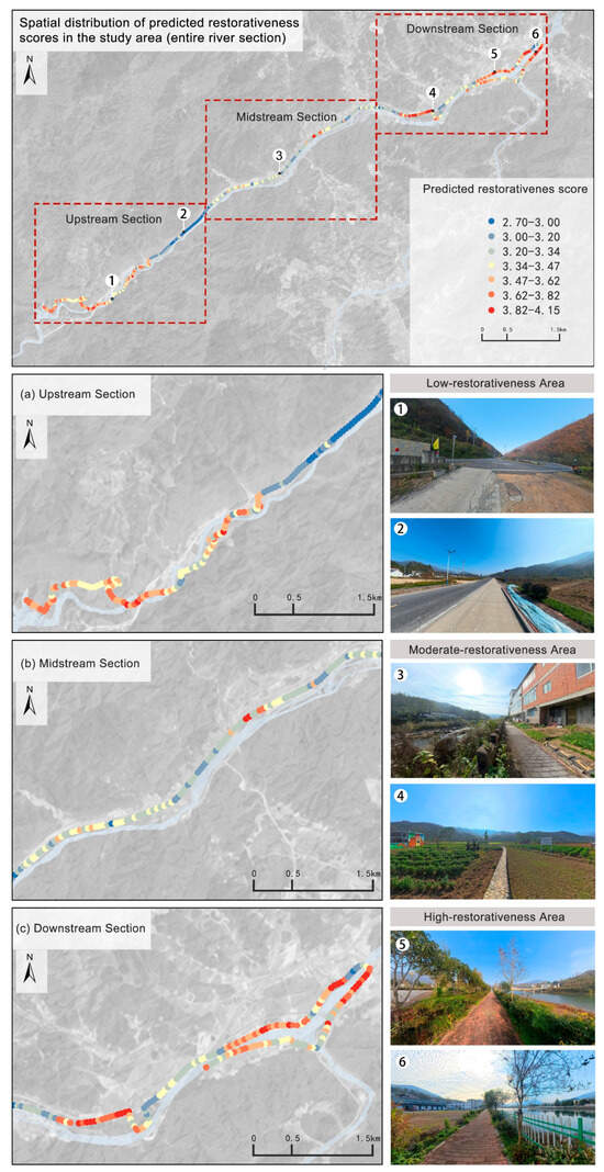
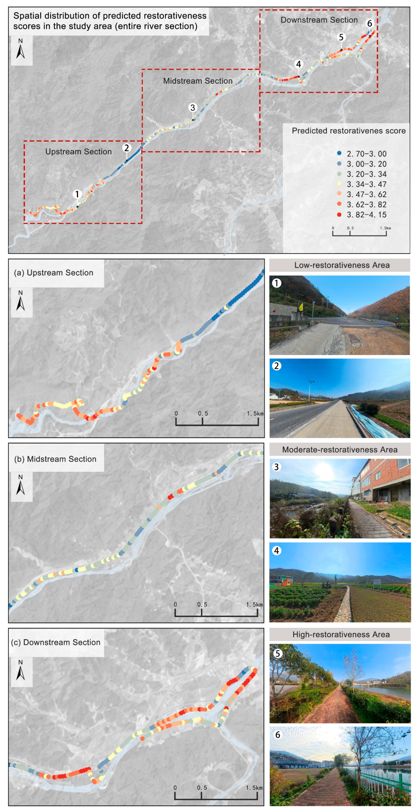
Based on the descriptive statistics and ArcGIS spatial visualization, the composite perceived-restorativeness scores under the low-water-level conditions surveyed in November 2025 showed an overall spatial pattern characterized by moderate scores in the upstream section, relatively lower scores in the midstream section, and relatively higher scores in the downstream section (Figure 5). In view of the leave-one-section-out results, this mapped pattern is interpreted as a relative description of variation within the surveyed corridor under the November 2025 survey conditions rather than as a spatially transferable classification of unobserved river sections. This pattern reflects the overall score distribution within each river section rather than a uniform classification of all sampling points within that section.

Figure 5. Spatial distribution of composite perceived restorativeness based on observed questionnaire ratings and random forest predictions. Numbers 1–6 mark the sampling locations corresponding to the photographs on the right.

The photographs numbered 1–6 in Figure 5 and their restorativeness categories represent only the local conditions at the displayed sampling points and do not indicate the overall category of the corresponding river section. Comparisons among river sections were based on the score distributions of all 215 sampling points. The spatial division into sections was used primarily to present relative differences within the continuous waterfront corridor rather than to treat the score categories as fixed attributes of the river sections.

Under the low-water-level conditions surveyed in November 2025, visible mountain and forest elements were relatively abundant in the upstream section, although some sampling points exhibited mountain-related visual obstruction and exposed bank slopes. Composite perceived-restorativeness scores in this section were generally moderate. At some midstream sampling points, the road visibility index, bare land visual ratio, and artificial structure visibility index were relatively high and were associated with relatively lower perceived-restorativeness scores. These findings reflect only the conditions of the present survey and should not be interpreted as fixed attributes of the river sections under other seasonal or water-level conditions.

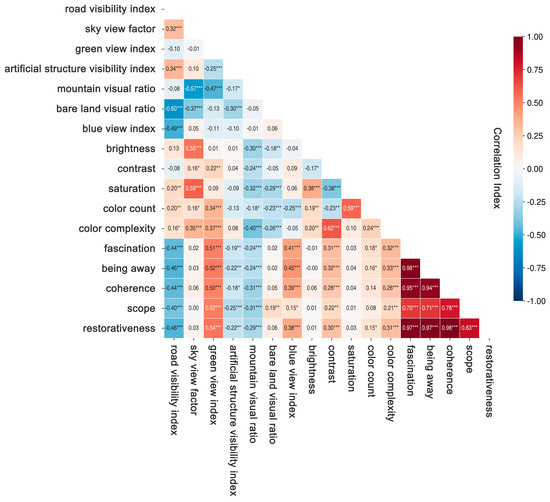
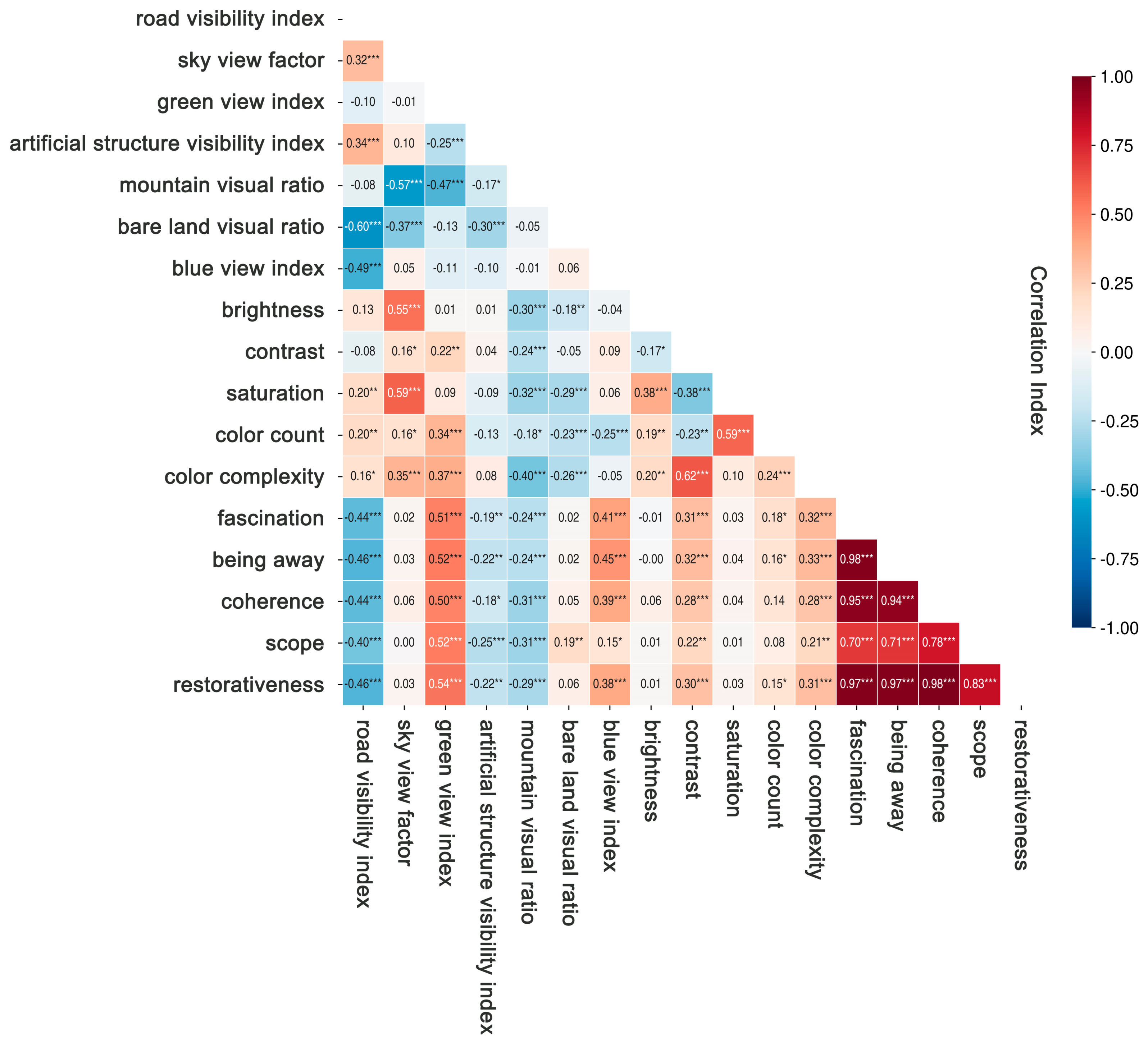
Correlation analysis showed that the green view index, blue view index, contrast, number of colors, and color complexity were significantly positively correlated with perceived restorativeness. In contrast, the road visibility index, mountain visual ratio, and artificial structure visibility index were significantly negatively correlated (Figure 6).

Figure 6. Heatmap of Pearson correlation coefficients between visual features and restorative perception. * p < 0.05, ** p < 0.01, and *** p < 0.001.

4. Discussion

4.1. Associations Between Visual Features and Perceived Restorativeness: Possible Explanations

This study found that the green view index, blue view index, contrast, number of colors, and color complexity were significantly positively correlated with perceived restorativeness. In contrast, the road visibility index, mountain visual ratio, and artificial structure visibility index showed significant negative correlations with perceived restorativeness. The Pearson correlations were calculated using the observed image-level mean scores of the 200 rated images rather than model-predicted scores. These findings are broadly consistent with previous studies of waterfront landscapes and urban green spaces [18,49]. They suggest that natural landscape elements and visually rich features were associated with higher perceived-restorativeness scores, whereas a high proportion of hardscape interfaces may be associated with lower perceived restorativeness [12,15,49]. These relationships may reflect how different landscape elements are associated with experiences of nature and visual perception in rural waterfront spaces.

Natural landscape elements provide an important foundation for perceived restorativeness in rural waterfront spaces. Both the green view index and blue view index were significantly positively correlated with perceived restorativeness. Images with greater visibility of vegetation and water tended to receive higher perceived-restorativeness scores. Previous studies have shown that vegetation and water provide rich natural visual information. They have also been associated with greater landscape attractiveness and restorative experiences [50,51]. Blue-green elements may be associated with greater perceived naturalness and stronger visual connections between people and nature. They may also be associated with more comfortable environmental experiences and higher perceived-restorativeness scores, although these possible pathways were not directly tested in this study. However, the median blue view index was 0 in this study. This result may reflect both the contraction of the water surface under the low-water-level conditions observed in November 2025 and viewpoint-related factors, including road orientation, riverbank morphology, foreground vegetation, and obstruction by artificial structures. Because repeated observations across multiple seasons were not conducted, the low blue view index should not be interpreted as a persistent structural characteristic of the river corridor. Under the present survey conditions, however, geographic proximity to the waterfront did not necessarily correspond to high water visibility. Under comparable site and seasonal conditions, waterfront landscape assessments could therefore examine water visibility along walking routes and at viewing locations. Where specific visual constraints are confirmed, planting configuration, waterfront spatial organization, and sightline management could be considered for site-specific evaluation.

Color features were also important correlates of perceived restorativeness. Contrast, number of colors, and color complexity were significantly positively correlated with perceived restorativeness. Images with greater color richness and layering tended to receive higher perceived-restorativeness scores, but this association does not demonstrate that increasing color richness would itself enhance landscape attractiveness. These findings are broadly consistent with previous landscape visual assessment studies. Existing research has reported associations between color variation, visual information richness, public perceptions of scenic beauty, and spatial quality [13,14,35]. By comparison, brightness and saturation showed weaker correlations with perceived restorativeness. Within the present dataset, perceived-restorativeness scores were more strongly associated with blue-green natural elements, color combinations, and overall landscape structure than with brightness or saturation. However, the positive relationships involving contrast, number of colors, and color complexity do not imply that artificial colors should be increased without limit. In mountainous rural waterfront landscapes, moderate color variation through seasonal changes, layered vegetation, and waterfront materials could be considered, although its effects would require site-specific evaluation.

Compared with natural landscape elements, built-environment factors showed an overall negative association with perceived restorativeness. The road visibility index was significantly negatively correlated with perceived-restorativeness scores. The artificial structure visibility index showed a weak but statistically significant negative correlation with perceived restorativeness. Previous studies have reported negative associations between intensive built development, landscape naturalness, and visual quality [18,52]. This pattern may reflect the visual disturbance associated with roads and hardscape facilities. Such features may coincide with interruptions in the natural continuity of rural waterfront environments and weaker visual connections between users and the natural setting. These possible explanations were not directly measured in this study. However, the high-scoring downstream areas also contained well-developed paths and recreational facilities. This important finding indicates that the presence of built facilities was not uniformly associated with low perceived-restorativeness scores. The functional value of built facilities should therefore be distinguished from their visual dominance. Planning strategies should not simply seek to reduce built facilities. Under comparable conditions, attention could instead be given to their scale, placement, visual prominence, and integration with waterfront vegetation and the surrounding landscape.

The mountain visual ratio showed a weak but statistically significant negative correlation with perceived restorativeness. This relationship may not be attributable to the mountain landscape itself. Instead, it may reflect the particular visual conditions of mountainous waterfront spaces. However, only the mountain visual ratio was measured directly; sightline obstruction, spatial openness, and visual depth were not independently quantified. Therefore, the possibility that riverside mountains obstruct sightlines or coincide with more enclosed views should be regarded as a contextual explanation rather than a directly measured result. Reduced slope vegetation and localized bare ground during autumn may also be associated with lower landscape continuity and integrity. These findings suggest that the relationship between the mountain visual ratio and perceived restorativeness is context-dependent. It may vary with spatial openness, vegetation cover, and sightline configuration.

Furthermore, the four dimensions of perceived restorativeness showed differences in the relative predictive importance of the landscape indicators. Random-forest feature importance was calculated as the normalized total reduction in squared-error impurity attributable to splits using each predictor across all trees, with the importance values summing to one within each model. These values represent relative predictive contributions rather than causal effects, and shared variation among predictors may distribute importance across correlated indicators. The random forest results showed that color indicators made relatively greater predictive contributions to coherence and scope. In contrast, bare land proportion was more important for predicting fascination and coherence. These differences suggest that perceived restorativeness cannot be attributed to a single landscape element. Instead, it appears to be associated with the combined configuration of natural elements, visual characteristics, and built-environment features. Given the substantial image-level overlap among fascination, being away, and coherence, these differences in predictor rankings are interpreted as exploratory patterns from the fitted models. They may be used to identify visual characteristics for further field verification but should not be interpreted as evidence of distinct dimension-specific predictor structures or causal mechanisms.

Beyond confirming previously reported associations involving blue-green elements and hardscape interfaces [18,32,49], this study provides two context-specific observations for mountainous rural waterfront corridors. First, under the low-water conditions observed in November 2025, proximity to the waterfront did not necessarily correspond to water visibility from pedestrian viewpoints. Second, relatively high perceived-restorativeness scores coexisted with well-developed paths and recreational facilities, indicating that infrastructure presence should be distinguished from its visible proportion and visual dominance. These findings support the use of pedestrian-view image analysis for diagnosing spatial variation within a continuous river corridor. However, the findings and planning implications are limited to the single study site and the November 2025 low-water survey conditions and require further multi-season and multi-site validation.

4.2. Implications for Rural Waterfront Landscape Development Based on Perceived Restorativeness Assessment

The results indicate that different landscape elements and their spatial configurations are differentially associated with perceived-restorativeness scores. Rural waterfront development should not focus solely on landscape beautification or facility provision. Greater attention should be given to public psychological responses to the spatial environment. During planning and implementation, perceived-restorativeness assessment could serve as an important reference for landscape planning and renewal. Objective visual indicators could be used to identify visual elements associated with lower perceived-restorativeness scores, and context-specific interventions could then be developed according to the landscape characteristics of different areas.

Perceived restorativeness also showed clear spatial variation across the study area. Rural waterfront development should therefore shift from uniform improvement toward zone-specific optimization. Priority should be given to areas with low restorativeness scores or pronounced visual problems. Renewal objectives can then be determined according to the main constraints in each area. This approach can improve the precision and relevance of landscape interventions.

For section-specific implementation, the middle section should prioritize road hardening, exposed riverbanks, and interfaces that obstruct water views. Small-scale improvements may include ecological paving, native vegetation buffers, and sightline enhancement. In the upstream section, the existing mountain forest landscape should be preserved. The causes of localized exposed slopes should also be examined. Viewpoints and walking routes can then be optimized in response to the terrain. Development priorities in each section should also be coordinated with flood safety, ecological conservation, and residents’ needs.

Semantic segmentation and machine learning can transform visual landscape features into quantitative indicators. They can also establish links between these indicators and public perceptions of restorativeness. Restorativeness assessment can therefore be incorporated into site diagnosis, design optimization, and post-construction evaluation. This approach can support a transition from experience-based judgment to data-assisted and fine-grained rural waterfront development.

It should be emphasized that these recommendations are derived from a cross-sectional analysis of a single river reach under the specific vegetation, water-level, and image-acquisition conditions observed in November 2025. Their applicability is therefore primarily limited to the study area and waterfront spaces with similar topographic, climatic, and usage conditions. Before implementation, the proposed measures should be further evaluated through multi-season surveys and field investigations while also considering flood-control safety, ecological protection, and villagers’ needs. Where feasible, small-scale pilot projects and before-and-after evaluations could be used to assess their practical effects.

4.3. Applicability of the Random Forest Model and Directions for Improvement

The R² values of the four restorative-dimension models ranged from 0.924 to 0.941 for the training set and from 0.719 to 0.732 for the hold-out test set, indicating that the random forest models captured nonlinear predictive relationships between the objective visual indicators and perceived restorativeness under the current sample conditions. Sampling-point-grouped five-fold cross-validation and leave-one-section-out validation were additionally conducted. The section-based results showed lower and section-dependent performance; therefore, the spatial outputs are interpreted as relative within-corridor patterns under the current survey conditions rather than as transferable predictions for unobserved sections.

Compared with traditional linear regression, random forest can capture nonlinear relationships and interactions among variables. Variable importance analysis can also identify indicators with high predictive contributions. These characteristics make random forest suitable for landscape perception assessments involving multiple indicators [44]. Compared with support vector machines, random forest generally places fewer demands on sample size and parameter tuning. It can therefore provide relatively stable performance with small to medium-sized datasets. Random forest is also simpler and more interpretable than deep learning methods such as convolutional neural networks [48]. It allows the relative predictive contributions of specific landscape indicators to be examined [18]. This feature is particularly useful for landscape assessment aimed at spatial optimization. Previous studies have applied random forest to landscape perception datasets containing approximately one hundred to several hundred samples [18,32]. In this study, responses from 300 valid questionnaires were aggregated into 200 image-level modeling samples. Five-fold cross-validation was used to characterize performance across data partitions. Within manageable small to medium-sized sampling conditions, random forest therefore provides a practical method for examining associations between objective visual indicators and perceived restorativeness. It can also provide quantitative support for restorativeness assessments of rural waterfronts and similar landscapes.

4.4. Research Limitations and Future Directions

The images used in this study were collected on 13 and 14 November 2025. Vegetation color, water-surface extent, exposed riverbanks, and mountain visibility may vary with seasonal and hydrological conditions. Therefore, the observed associations and spatial scoring patterns primarily apply to the conditions of this survey. Their transferability to summer conditions or different water levels requires further validation. The current models have not been independently tested in other watersheds. Accordingly, the transferable contribution of this study lies in its assessment and spatial diagnosis workflow. The model parameters and scoring thresholds should not be assumed to apply universally.

All semantic segmentation results were manually inspected; however, independent manually annotated pixel-level ground-truth masks were not created. Future studies could manually annotate representative images selected from different river sections and landscape types and report class-specific intersection-over-union (IoU) and F1 scores to further validate the model’s segmentation performance in mountainous rural waterfront environments.

This study retained the established four-dimensional structure of the PRS-11. Fascination, being away, and coherence reflect interrelated psychological experiences in perceptions of restorative environments, and their high correlations may be associated with the theoretical structure and item content of the scale. Therefore, the four-dimensional framework was retained, while differences among the first three dimensions were interpreted cautiously. Future studies could include common anchor images across questionnaire versions, record and control for device type and screen conditions, and use larger samples to further examine the dimensional structure and rating stability. In addition, the questionnaire imposed no restrictions on the response device, and most respondents used smartphones. Respondents’ familiarity with the study site and degree of response fatigue were not recorded, and no common anchor images were included across questionnaire versions. These factors may affect comparability among versions and should be controlled in future research.

This study focused on typical rural waterfront spaces in the low-mountain and hilly areas of the Jianghuai region. The study area is located within a subtropical-temperate climatic transition zone. Future research should include a wider range of landforms and climatic regions. Comparative studies across rural waterfront environments may improve model transferability and generalizability. To clarify the contribution of visual information to perceived restorativeness, this study relied mainly on two-dimensional static images. Future assessments could incorporate multisensory environmental information, including sound and smell. This would broaden the dimensions of perceived restorativeness and improve the comprehensiveness of the assessment. The present study used real-world photographs as experimental materials. Future research could combine virtual reality with eye-tracking and physiological-response data. These approaches may reduce manual data-collection costs and support controlled simulation experiments.

5. Conclusions

Using panoramic imagery, deep-learning-based semantic segmentation, and random forest regression, this study developed a framework for assessing perceived restorativeness in mountainous rural waterfront landscapes by integrating landscape elements and color features. Its main contribution lies in combining 12 interpretable objective visual indicators with the four PRS-11 dimensions and applying image-level assessments of perceived restorativeness to the spatial diagnosis of a continuous waterfront corridor, thereby providing a feasible approach for evaluating rural waterfront landscapes under complex terrain conditions. The models demonstrated internal predictive capacity under the current sample conditions. Given the substantial image-level overlap among fascination, being away, and coherence, differences in predictor rankings across the four fitted models are interpreted as exploratory patterns rather than as evidence of distinct dimension-specific predictor structures. Overall, the visibility of blue–green landscape elements and color richness was associated with higher perceived-restorativeness scores, whereas images with higher road visibility index, mountain visual ratio, and artificial structure visibility index values tended to receive lower scores. These findings are specific to the dry-season and low-water-level conditions surveyed in November and require further validation before being generalized to other seasons or water-level conditions. In particular, without repeated multi-season observations, the low blue view index should not be interpreted as a persistent structural characteristic. Based on these findings, landscape optimization under comparable conditions could focus on the visibility of blue–green elements, the layering of native vegetation, and pedestrian sightline conditions. The results may provide an evidence-based reference for restorativeness-oriented planning and design of mountainous rural waterfront landscapes.

References

- Li, Y.R.; Cao, L.Z.; Wang, P.Y.; Chang, G.J. Rural living environment improvement and rural revitalization. J. Nat. Resour. 2022, 37, 96–109. [Google Scholar] [CrossRef] [Scilit]
- Li, B.H.; Yang, F.D.; Dou, Y.D. The organic renewal of the human settlement environment in traditional villages: Theoretical cognition and practical path. Geogr. Res. 2022, 41, 1407–1421. [Google Scholar] [CrossRef]
- Nie, W.; Zhu, R.K.; Xu, Y.R.; Li, G. Research and Practice of Rural Landscape Control Strategy from the Perspective of Harmonious and Beautiful Countryside: Taking Jinzhai County in Anhui Province as an Example. Dev. Small Cities Towns 2024, 42, 28–35. [Google Scholar] [CrossRef]
- Li, X.; Wang, Y.; Wang, Z.; Ding, Q. Evaluation of the visual perception of urban single/double-layer riverfront greenway landscapes based on deep learning. Sustainability 2024, 16, 10391. [Google Scholar] [CrossRef] [Scilit]
- Xia, Y.; Yabuki, N.; Fukuda, T. Development of a system for assessing the quality of urban street-level greenery using street view images and deep learning. Urban For. Urban Green. 2021, 59, 126995. [Google Scholar] [CrossRef] [Scilit]
- Jain, J.; Li, J.; Chiu, M.T.; Hassani, A.; Orlov, N.; Shi, H. OneFormer: One Transformer to Rule Universal Image Segmentation. In Proceedings of the IEEE/CVF Conference on Computer Vision and Pattern Recognition (CVPR), Vancouver, BC, Canada, 18–22 June 2023; pp. 2989–2998. [Google Scholar] [CrossRef] [Scilit]
- Wang, J.Q.; Jiang, H.Q.; Chen, J.Y.; Ke, N.; Wang, M. Identification of Autumn Landscape Characteristics and Vitality Improvement in Urban Waterfront Spaces Based on Artificial Intelligence: A Case Study of Huangpu River in Shanghai. Chin. Landsc. Archit. 2024, 40, 15–21. [Google Scholar] [CrossRef]
- Zhang, M.K.; Wang, S.Y.; Jin, Y. Study on Visual Landscape Value of Waterfront Green Space in Qiantang River Basin. Archit. Cult. 2025, 2, 92–94. [Google Scholar] [CrossRef]
- Mo, S.; Dai, Z.; Wen, Y. Study on rural landscape design strategies integrating computer vision and deep learning: An analysis based on human perception and visual aesthetics. Sci. Rep. 2025, 15, 35722. [Google Scholar] [CrossRef] [Scilit]
- Zhai, Y.J.; Lu, Y.Z.; Yu, J.Y.; Zhang, X.; Luo, T.Q. Perception Preference and Improvement Strategy for the Waterfront Space of Suzhou Creek of Shanghai Based on Deep Learning. Hous. Sci. 2025, 45, 17–25. [Google Scholar] [CrossRef]
- Li, L.; Lange, K.W. Assessing the relationship between urban blue-green infrastructure and stress resilience in real settings: A systematic review. Sustainability 2023, 15, 9240. [Google Scholar] [CrossRef] [Scilit]
- Zhao, X.K.; Lin, G.S. Research on the perception evaluation of urban green spaces using panoramic images and deep learning: A case study of Zhujiang Park in Guangzhou. Landsc. Archit. Front. 2024, 12, 7–18. [Google Scholar] [CrossRef] [Scilit]
- Liu, C.; Wang, T.-Y.; Yuizono, T. Assessing the landscape visual quality of urban green spaces with multidimensional visual indicators. Urban For. Urban Green. 2025, 106, 128727. [Google Scholar] [CrossRef] [Scilit]
- Fang, Y.-N.; Tian, J.; Namaiti, A.; Zhang, S.; Zeng, J.; Zhu, X. Visual aesthetic quality assessment of the streetscape from the perspective of landscape-perception coupling. Environ. Impact Assess. Rev. 2024, 106, 107535. [Google Scholar] [CrossRef] [Scilit]
- Zhou, X.; Xu, H.Y. Research on the Visual Landscape Quality Assessment of Qinhuai River Waterfront Landscape in Nanjing with the Support of Image Deep Learning Technology. Chin. Landsc. Ahirct. 2022, 38, 84–87. [Google Scholar] [CrossRef]
- Li, C.X.; Ye, L.Q.; Li, R. The influence of restorative environment perception in rural tourism on tourist experience quality: The multiple mediation models. J. Resour. Ecol. 2024, 15, 1653–1665. [Google Scholar] [CrossRef] [Scilit]
- Sun, D.; Yang, Q.R.; Hao, W.H.; Ji, X.; Lyu, M. Research on the Landscape Measurement Characteristics and the Visual Perception Evaluation of the Seaside Bathing Beaches in Qingdao. Landsc. Des. 2025, 23, 18–21. [Google Scholar] [CrossRef]
- Li, X.; Li, L.; Wang, X.; Lin, Q.; Wu, D.; Dong, Y.; Han, S. Visual quality evaluation model of an urban river landscape based on random forest. Ecol. Indic. 2021, 133, 108381. [Google Scholar] [CrossRef] [Scilit]
- Li, G.; Wang, H.; Zhang, F.Q.; Qi, Y.X.; Yang, Z.C.; Yang, Y.; Nie, W. Evaluation Methodology for Scenic Beauty in Wetland Parks Utilizing Open Data and Analysis of Influencing Factors: A Case Study of the Lake Chaohu Wetland Park Group. Landsc. Archit. Acad. J. 2025, 42, 52–60. [Google Scholar] [CrossRef]
- Ji, G.; Sun, H. Assessing urban river landscape visual quality with extreme learning machines: A case study of the Yellow River in Ningxia Hui Autonomous Region, China. Ecol. Indic. 2024, 165, 112173. [Google Scholar] [CrossRef] [Scilit]
- Zhang, K.L.; Li, Q.Y.; Wei, W.; Zhang, X.Y.; Zhou, H.D. Exploring the Research Mode of Landscape Architecture in Colleges to Help Rural Revitalization: A Study of Rural Landscape in Ju River Basin, Huangling County, Shaanxi Province. J. Beijing For. Univ. Soc. Sci. 2023, 22, 85–93. [Google Scholar] [CrossRef]
- Long, J.R.; Zhang, Y.N.; Zhang, X.B.; Li, J. Nature-based solutions and rural spatial restructuring: A systematic review. Prog. Geogr. 2025, 44, 670–683. [Google Scholar] [CrossRef] [Scilit]
- Zhang, C.; Tang, Y.L.; Guo, T.T.; Zhang, J.; Fu, D.S.; Xing, Y.; Yang, Y.F.; Shao, F. Study on Relationship between Landscape Feature of Qingshanhu Lake Waterfront Greenway and Aesthetic Perception. J. Zhejiang For. Sci. Technol. 2023, 43, 74–81. [Google Scholar] [CrossRef]
- Zhang, F.; Zhou, B.; Liu, L.; Liu, Y.; Fung, H.H.; Lin, H.; Ratti, C. Measuring human perceptions of a large-scale urban region using machine learning. Landsc. Urban Plan. 2018, 180, 148–160. [Google Scholar] [CrossRef] [Scilit]
- Wu, Y.; Qiu, H.F.; Luo, X.Y.; Hu, Y.P. Impact of Urban Waterfront Green Space Landscape Elements on Public Health Behaviors Based on Restorative Perception. Landsc. Archit. 2025, 32, 119–126. [Google Scholar] [CrossRef] [Scilit]
- Li, Y.; Yabuki, N.; Fukuda, T. Measuring visual walkability perception using panoramic street view images, virtual reality, and deep learning. Sustain. Cities Soc. 2022, 86, 104140. [Google Scholar] [CrossRef] [Scilit]
- Wilkins, E.J.; Van Berkel, D.; Zhang, H.; Dorning, M.A.; Beck, S.M.; Smith, J.W. Promises and pitfalls of using computer vision to make inferences about landscape preferences: Evidence from an urban-proximate park system. Landsc. Urban Plan. 2022, 219, 104315. [Google Scholar] [CrossRef] [Scilit]
- Zhou, B.; Zhao, H.; Puig, X.; Xiao, T.; Fidler, S.; Barriuso, A.; Torralba, A. Semantic Understanding of Scenes through the ADE20K Dataset. Int. J. Comput. Vis. 2019, 127, 302–321. [Google Scholar] [CrossRef] [Scilit]
- Fei, T.T.; Hua, Y.Y.; Wang, J.H.; Zhou, W.Q. Urban Visual Environment and Human Responses: An Analytical Framework and Systematic Review. Landsc. Archit. 2026, 33, 20–28. [Google Scholar] [CrossRef] [Scilit]
- Xia, Y.; Yabuki, N.; Fukuda, T. Sky view factor estimation from street view images based on semantic segmentation. Urban Clim. 2021, 40, 100999. [Google Scholar] [CrossRef] [Scilit]
- Luo, J.; Zhao, T.; Cao, L.; Biljecki, F. Semantic Riverscapes: Perception and evaluation of linear landscapes from oblique imagery using computer vision. Landsc. Urban Plan. 2022, 228, 104569. [Google Scholar] [CrossRef] [Scilit]
- Qiu, W.; Li, W.; Liu, X.; Zhang, Z.; Li, X.; Huang, X. Subjective and objective measures of streetscape perceptions: Relationships with property value in Shanghai. Cities 2023, 132, 104037. [Google Scholar] [CrossRef] [Scilit]
- Chang Chien, Y.-M.; Carver, S.; Comber, A. Using geographically weighted models to explore how crowdsourced landscape perceptions relate to landscape physical characteristics. Landsc. Urban Plan. 2020, 203, 103904. [Google Scholar] [CrossRef] [Scilit]
- Schüpbach, B.; Roesch, A.; Herzog, F.; Szerencsits, E.; Walter, T. Development and application of indicators for visual landscape quality to include in life cycle sustainability assessment of Swiss agricultural farms. Ecol. Indic. 2020, 110, 105788. [Google Scholar] [CrossRef] [Scilit]
- Cao, Y.; Yang, P.; Xu, M.; Li, M.; Li, Y.; Guo, R. A novel method of urban landscape perception based on biological vision process. Landsc. Urban Plan. 2025, 254, 105246. [Google Scholar] [CrossRef] [Scilit]
- Gonzalez, R.C.; Woods, R.E. Digital Image Processing, 4th ed.; Pearson: New York, NY, USA, 2018. [Google Scholar]
- Smith, A.R. Color gamut transform pairs. ACM SIGGRAPH Comput. Graph. 1978, 12, 12–19. [Google Scholar] [CrossRef] [Scilit]
- Swain, M.J.; Ballard, D.H. Color indexing. Int. J. Comput. Vis. 1991, 7, 11–32. [Google Scholar] [CrossRef] [Scilit]
- Shannon, C.E. A mathematical theory of communication. Bell Syst. Tech. J. 1948, 27, 379–423. [Google Scholar] [CrossRef] [Scilit]
- Sousa, C.; Fernandes, M.J.; Encarnação, T.; Gonçalves, G. Adaptation and validation of the Perceived Restorativeness Scale (PRS) for the Portuguese population: A study on the assessment of the restorative effect of environments. Green Health 2025, 1, 7. [Google Scholar] [CrossRef] [Scilit]
- Pasini, M.; Berto, R.; Brondino, M.; Hall, R.; Ortner, C. How to measure the restorative quality of environments: The PRS-11. Procedia Soc. Behav. Sci. 2014, 159, 293–297. [Google Scholar] [CrossRef] [Scilit]
- Biau, G.; Scornet, E. A random forest guided tour. TEST 2016, 25, 197–227. [Google Scholar] [CrossRef] [Scilit]
- Probst, P.; Wright, M.N.; Boulesteix, A.-L. Hyperparameters and tuning strategies for random forest. WIREs Data Min. Knowl. Discov. 2019, 9, e1301. [Google Scholar] [CrossRef] [Scilit]
- Breiman, L. Random forests. Mach. Learn. 2001, 45, 5–32. [Google Scholar] [CrossRef] [Scilit]
- Stone, M. Cross-validatory choice and assessment of statistical predictions. J. R. Stat. Soc. Ser. B 1974, 36, 111–133. [Google Scholar] [CrossRef] [Scilit]
- Guo, H.G.; Zhang, M.H.; Wan, B.Y.; Hong, X.C. A Machine Learning-Based Research on the Influence of Street Environment Colors on the Elderly’s Perception of Pleasure. Landsc. Archit. 2025, 32, 119–127. [Google Scholar] [CrossRef] [Scilit]
- Willmott, C.J.; Matsuura, K. Advantages of the mean absolute error (MAE) over the root mean square error (RMSE) in assessing average model performance. Clim. Res. 2005, 30, 79–82. [Google Scholar] [CrossRef] [Scilit]
- Linardatos, P.; Papastefanopoulos, V.; Kotsiantis, S. Explainable AI: A review of machine learning interpretability methods. Entropy 2021, 23, 18. [Google Scholar] [CrossRef] [Scilit]
- Xiong, X.; Wen, X.Y.; Yang, S.R.; Liu, L.; Zeng, W. Visual Quality Assessment and Influencing Factors Analysis of Urban Waterfront Greenway Landscape: A Case Study of Nanjing Jiajiang Riverside Greenway. Landsc. Archit. Acad. J. 2024, 41, 69–77. [Google Scholar] [CrossRef]
- Kaplan, S. The restorative benefits of nature: Toward an integrative framework. J. Environ. Psychol. 1995, 15, 169–182. [Google Scholar] [CrossRef] [Scilit]
- Ulrich, R.S. View through a window may influence recovery from surgery. Science 1984, 224, 420–421. [Google Scholar] [CrossRef] [Scilit]
- Yu, M.; Chen, X.; Zheng, X.; Cui, W.; Ji, Q.; Xing, H. Evaluation of spatial visual perception of streets based on deep learning and spatial syntax. Sci. Rep. 2025, 15, 18439. [Google Scholar] [CrossRef] [Scilit]
Disclaimer/Publisher’s Note: The statements, opinions and data contained in all publications are solely those of the individual author(s) and contributor(s) and not of MDPI and/or the editor(s). MDPI and/or the editor(s) disclaim responsibility for any injury to people or property resulting from any ideas, methods, instructions or products referred to in the content. |
© 2026 by the authors. Licensee MDPI, Basel, Switzerland. This article is an open access article distributed under the terms and conditions of the Creative Commons Attribution (CC BY) license.