Digital Spatial Governance and Built-Up Land Carbon Intensity: Evidence from China’s Smart City Pilot Program

Abstract

Smart city policies may affect urban carbon emissions and developed land at the same time, but the two may not change in the same direction. This study examines city-level carbon dioxide (CO₂) emissions per unit of built-up land area, whose natural logarithm is denoted as lnCLCI using panel data for 40 cities in the middle reaches of the Yellow River Basin and surrounding areas from 2011 to 2022. The main policy sample includes 37 cities after removing three cases where the Smart City Pilot designation covered only a sub-prefectural area. Treatment timing is defined using the actual adoption year of each city. Group-time average treatment effects are used as the main estimates, while a two-way fixed-effects model serves as a benchmark. The analysis also separates the responses of carbon emissions and built-up land, tests spatial policy exposure and pre-policy heterogeneity, and evaluates prediction performance in cities excluded from model training. The unadjusted group-time average treatment effect is 0.026 with a p-value of 0.708. After adjustment for pre-treatment covariates, the estimate is −0.040 with a p-value of 0.673. The TWFE benchmark gives an estimate of 0.008 with a p-value of 0.909. These estimates do not provide evidence that the Smart City Pilot policy reduced lnCLCI on average. Estimates for log carbon emissions (lnCO₂) and log built-up land area (lnBUA) are also statistically imprecise, and the pre-policy interaction tests show no consistent pattern of treatment heterogeneity. Estimates of spatial policy exposure are sensitive to the choice of spatial weight matrix. In the 2013–2022 prediction sample, Random Forest achieves a held-out-city R² of 0.568, compared with 0.767 for OLS. Taken together, the results show that changes in carbon emissions per unit of built-up land should not be interpreted as changes in absolute emissions alone. They also show the importance of keeping predictive performance separate from estimates of policy effects.

1. Introduction

Urban carbon policy concerns not only energy use but also the spatial organization of cities. Digital infrastructure, sensing systems, and data platforms can reduce some operating costs through monitoring and information sharing, yet they also require energy and can attract additional activity. The net carbon effect of smart city development is an empirical question. China’s Smart City Pilot Program provides a policy setting in which that effect can be studied from observed adoption dates [1].

Smart city pilots combine digital infrastructure with local governance and public services. Existing studies of China’s Smart City Pilot Program have mainly examined energy efficiency, carbon emissions, and green development [2,3,4,5,6,7]. These outcomes do not fully describe the relationship between urban carbon emissions and land development because emissions and built-up land may change at different rates [8,9,10,11].

This study therefore focuses on carbon emissions per unit of built-up land and reports changes in carbon emissions and built-up land separately to clarify the source of changes in the ratio. The analysis uses a panel of 40 prefecture-level cities in the middle reaches of the Yellow River Basin and adjacent areas. The sample includes regional centers, traditional industrial cities, and resource-dependent cities, with substantial differences in population density and patterns of land development [8,9,10,11,12]. It represents a specific regional setting rather than a nationally representative sample. Built-up land carbon intensity is used as a land-normalized carbon measure and is not treated as a substitute for total carbon emissions or carbon intensity per unit of GDP.

The main analysis tests whether Smart City Pilot designation changes carbon emissions per unit of built-up land. It also examines whether exposure to nearby designated cities is associated with this outcome and whether observed city characteristics can predict differences across cities. The policy analysis accounts for differences in treatment timing and administrative coverage, while the prediction analysis evaluates performance in cities excluded from model fitting.

2. Literature Review and Research Gap

2.1. Smart Cities and Low-Carbon Development

Existing studies have examined the effects of smart city policies on energy efficiency, carbon emissions, carbon productivity, and green development [2,3,4,5,6,7]. Their findings are not always consistent, partly because studies use different outcomes, treatment definitions, and identification strategies. These differences are particularly important for policies introduced at different times across cities, as treatment timing affects which observations are used to estimate the average policy effect.

Digitalization itself does not necessarily reduce carbon emissions. Digital monitoring and improved resource allocation may lower energy waste, but data centers, computing infrastructure, and expanding digital activities also increase electricity demand. Recent studies therefore find nonlinear relationships between computing infrastructure and carbon intensity, as well as different responses of total carbon emissions and emission intensity [13,14,15,16,17,18,19,20]. The carbon effect of a smart city policy cannot be inferred from the level of digitalization alone and needs to be estimated from the policy change itself.

Related evidence also comes from China’s national smart-tourism pilot, where digital transformation has been linked to urban carbon-emission efficiency [21]. That program differs from the Smart City Pilot in both policy setting and outcome definition. Its findings are relevant to the broader low-carbon digitalization literature, but they do not establish the effect of Smart City Pilot designation on carbon emissions per unit of built-up land.

2.2. Urban Spatial Carbon Efficiency from a Land-Use Perspective

Land development shapes where urban activities occur and how much energy they require. The expansion and density of built-up land, infrastructure layout, and commuting distance are closely related to population distribution and urban energy demand [8,9,10,11,22,23,24,25,26]. Carbon emissions per unit of GDP measure emissions relative to economic output, whereas built-up land carbon intensity measures emissions relative to developed land area. The latter therefore reflects the carbon emissions associated with each unit of built-up space.

Recent studies on smart cities and digitalization have increasingly examined land-use efficiency and green land-use efficiency [27,28,29,30,31,32,33]. These measures usually combine multiple inputs and outputs and capture a broader concept of land-use performance. Carbon emissions per unit of built-up land have a narrower meaning because the ratio is determined directly by total emissions and built-up land area. An increase in built-up land can reduce the ratio even when total carbon emissions increase. To avoid interpreting a lower ratio as an automatic reduction in emissions, this study reports lnCO₂ and lnBUA separately and uses lnCLCI as a complementary measure of the carbon burden associated with urban land development.

2.3. Spatial Externalities, Staggered Policy Adoption, and Interpretable Machine Learning

Smart city policies may be associated with outcomes outside the treated city. Policy learning, technology diffusion, and supply-chain connections can link nearby cities, while industrial relocation and the movement of capital and labor may shift carbon-intensive activities across city boundaries. These processes can work in different directions, so the sign of the cross-city association is not determined in advance [34,35,36,37].

This study measures cross-city policy exposure using several spatial weight matrices, each representing a different form of connection between cities [34]. The resulting spatial estimates are treated as robustness and specification checks rather than direct evidence of technology diffusion or industrial relocation. Policy timing is addressed separately. Conventional TWFE estimates may mix comparisons across treatment cohorts when policy effects vary over time [38,39,40,41,42,43,44]. Group-time average treatment effects and an interaction-weighted event-study specification are therefore used to account for staggered treatment timing. Random Forest, RFECV, and SHAP serve a different purpose: they are used only to assess predictive performance, select predictors, and describe model-based variable contributions, not to estimate policy effects [45,46,47,48,49,50,51].

3. Theoretical Mechanisms and Research Hypotheses

3.1. Local Effects: Digital Governance and Spatial Resource Allocation

Smart city pilots can change how urban information is collected and used in daily management. Real-time monitoring, data platforms, and information sharing across departments may improve the operation of transport systems, energy supply, public buildings, and municipal services [13,20,52,53]. Better coordination can reduce idle capacity, repeated construction, and other forms of inefficient resource use, which may lower both energy consumption and unnecessary land expansion. Digital infrastructure, however, also creates additional energy demand. Data centers, communication networks, smart terminals, and computing services require continuous electricity, while better public services and business conditions may attract more population and economic activity [54,55,56,57,58,59,60,61,62,63]. These changes can increase both emissions and demand for developed land. The overall effect on built-up land carbon intensity is therefore uncertain and depends on how the emissions response compares with the change in built-up land area.

H1. 

Smart City Pilot designation reduces local built-up land carbon intensity.

3.2. Spatial Externalities: Green Diffusion and the Relocation of Carbon-Intensive Activities

Cross-city effects may arise through several channels. Digital standards, green technologies, and governance practices can spread through firm networks, supply chains, and policy learning [2,3,4,5,7,12,64,65]. Such diffusion may improve resource use and reduce carbon pressure in nearby cities [66,67,68]. Policy changes can also alter land costs, regulatory conditions, and environmental constraints, encouraging energy-intensive or land-intensive activities to relocate across city boundaries. In that case, neighboring cities may face higher carbon pressure. These two processes can produce effects in opposite directions. The spatial analysis therefore tests whether exposure to nearby Smart City Pilot cities is associated with lnCLCI, but it does not infer a specific transmission mechanism from the spatial weight matrix alone.

H2. 

Smart City Pilot designation is associated with cross-city changes in built-up land carbon intensity, with the direction depending on the balance between green diffusion and the relocation of carbon-intensive activities.

3.3. Channels: Digital–Intelligent Integration, Energy Use, and Intensive Land Use

Digital systems can improve the coverage and timeliness of information on energy use, transport, infrastructure, and land development. Better information may help local governments allocate resources more closely to actual demand. A composite digital–intelligence integration index (DII) can be used to describe this dimension, but changes in the index cannot by themselves establish a mediation pathway. In the present dataset, pre-policy DII values are unavailable for the first treatment cohort, which further limits formal channel identification.

H3a. 

Smart City Pilot designation increases digital–intelligent integration. This hypothesis is treated as a theoretical proposition because pre-policy DII values are unavailable for the first treatment cohort.

Energy intensity (EI), defined as energy use per unit of GDP, provides a related outcome for empirical examination. Smart energy management, load monitoring, and equipment scheduling can reduce unnecessary operation when energy use is adjusted to actual demand. If this mechanism is present, energy intensity should decline after pilot adoption and move in the same direction as lnCLCI.

H3b. 

Smart City Pilot designation reduces energy intensity, and a decline in energy intensity is consistent with a reduction in built-up land carbon intensity.

Digital land records and more coordinated public services may also change how intensively existing urban space is used [27,33]. To examine this possibility, the analysis considers GDP per unit of built-up land, resident population per unit of built-up land, and annual built-up land growth. These variables are treated as related outcomes rather than formal mediators because they either share the same land denominator as lnCLCI or are constructed directly from built-up land area. INS is excluded because its original construction cannot be recovered from the archived data.

H3c. 

Smart City Pilot designation is associated with higher population accommodation on existing built-up land and slower built-up land expansion. These relationships are interpreted as related policy responses rather than evidence of mediation.

3.4. The Conditional Role of Urban Density

Smart city infrastructure often involves fixed investment costs that are shared across the population and activities served by the system. In denser cities, monitoring platforms, communication networks, and related digital infrastructure can serve more users within a smaller area. Similar systems in lower-density cities must cover more land per user, which may affect both energy use and the land response to the policy [23,25,26]. The analysis tests this possibility using population-density groups defined before policy adoption. Pre-policy density is used to avoid classifying cities with a variable that may itself respond to treatment.

H4. 

The reduction in built-up land carbon intensity associated with Smart City Pilot designation is stronger in cities with higher pre-policy population density.

4. Methods

4.1. Sample and Data Sources

The balanced panel covers 40 prefecture-level cities from 2011 to 2022, yielding 480 city-year observations. The preferred policy sample excludes Luoyang, Lüliang, and Baotou because the available pilot records identify a district, county, or new town rather than the prefecture-level city as the treatment unit. After these exclusions, the main sample contains 37 cities and 444 observations, including 18 treated cities and 19 cities that were never treated. City names and numeric identifiers are checked against the policy records before treatment status and adoption year are assigned. Results based on all 40 cities are retained as sensitivity checks for the definition of treatment scope.

4.2. Data and Variable Construction

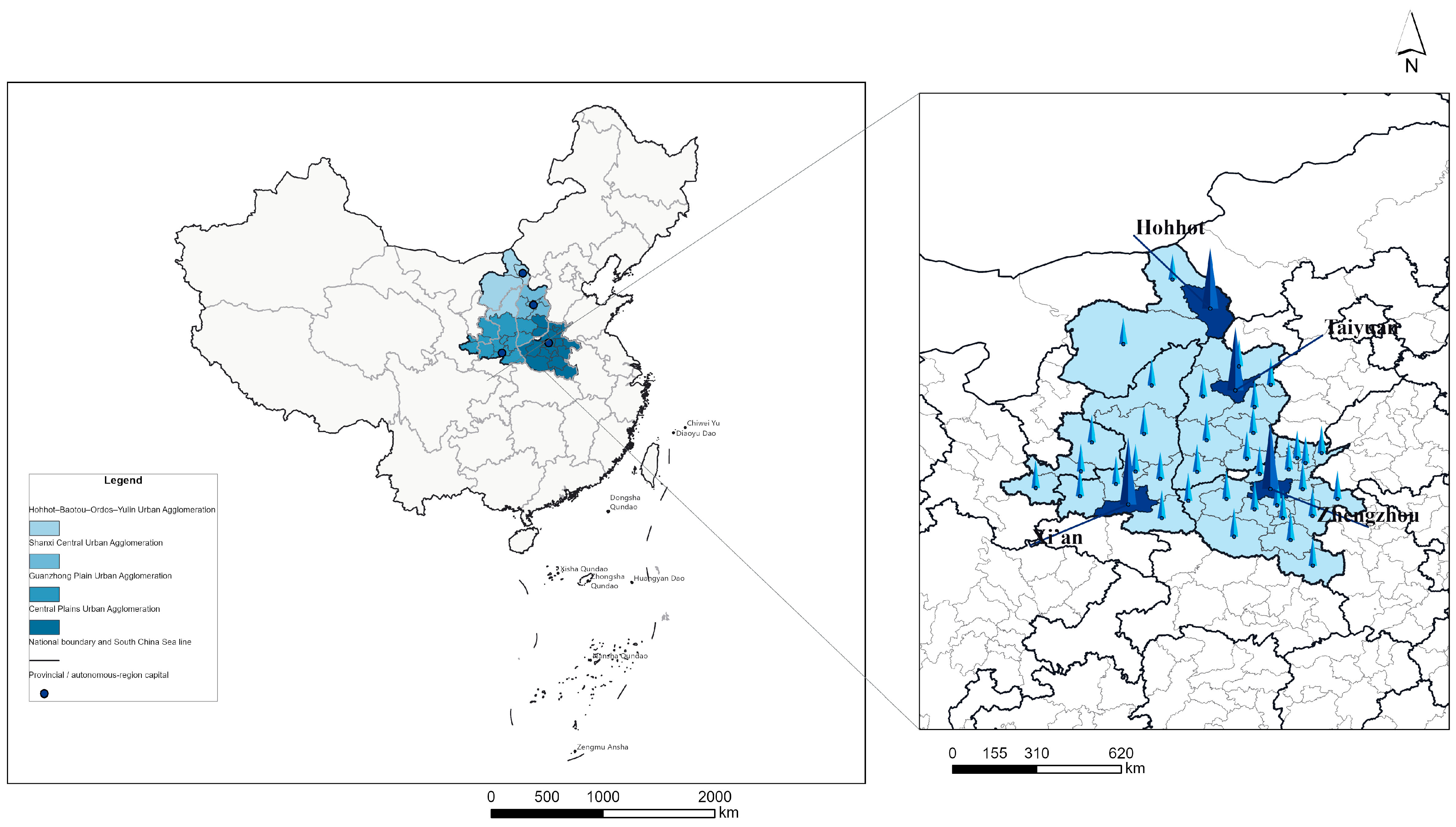
Figure 1 shows the location of the 40-city research area and places the regional sample within China. The map is descriptive and also provides the spatial frame used to construct the geographic weight matrices; the preferred policy analysis subsequently excludes the three sub-prefectural pilot cases described in Section 4.1. SCP equals one from the year of valid whole-city designation onward and zero otherwise. Cities with a zero or missing adoption year are treated as never treated. According to the compiled policy records, 13 cities entered the program in 2013 and five in 2015. These dates follow the announcement-year convention used in the archive and indicate policy designation rather than the intensity of implementation. As a sensitivity check, a broader treatment definition assigns the three sub-prefectural pilots to their corresponding prefecture-level cities. The preferred definition retains only whole-city designations so that the policy unit is consistent with the city-level outcome. This restriction does not exclude the possibility that sub-city pilots in comparison cities generated some local exposure.

Figure 1. Location and overview of the research area (Map Approval No. GS(2020)4619).

The dependent variable, lnCLCI, is the natural logarithm of city-level CO₂ emissions divided by built-up land area (BUA). Across the full sample of 480 city-year observations, the stored lnCLCI values equal lnCO₂ minus lnBUA to numerical precision. The source files report CO₂ emissions in tonnes and built-up land area in square kilometers, so the corresponding unlogged measure is expressed as tonnes of CO₂ per square kilometer of built-up land. The archived land worksheet labels BUA as built-up land area, but the available records do not preserve a more detailed operational definition or classification rule for what is included as built-up land. The land-use worksheet states that linear interpolation was applied, but it does not identify the individual observations that were interpolated. The emissions series is compiled at the city level, and the archived materials do not indicate that emissions are limited to activities physically located within built-up parcels. CLCI is therefore interpreted as total city emissions normalized by built-up land area rather than as emissions produced within built-up land itself. The variable-definition sheet refers to coal, oil, and natural gas and provides an example based on a standard-coal carbon factor. However, the archived materials do not retain the complete fuel-specific calculation sheet, the carbon-to-CO₂ conversion procedure, electricity accounting, or the full inventory boundary. The upstream emissions inventory therefore cannot be fully reconstructed from the available files.

The benchmark controls include the natural logarithms of fixed-asset investment, green patent authorizations, GDP, and administrative population density, together with the fiscal and urbanization measures provided in the dataset. Group-time treatment effects are estimated both without covariates and with covariate adjustment based only on pre-treatment values. Current investment, patent activity, GDP, and population density are not used for adjustment because they may themselves respond to Smart City Pilot designation. Energy intensity is measured as ten thousand tonnes of standard coal per hundred million yuan of GDP. GDP per unit of built-up land, resident population per unit of built-up land, and annual built-up land growth are reconstructed from the underlying component data. Resident population is converted from ten thousand persons to persons before population per built-up land area is calculated. Table 1 summarizes the measurement, unit or transformation, and available data provenance for the variables used in the empirical analysis.

Table 1. Variable definitions and data sources.

Variable	Measurement	Data Provenance
lnCLCI	lnCO2—lnBUA; CO2 in tonnes and BUA in km2	Archived city emissions and land-area workbooks; upstream emission inventory and detailed BUA operational definition incomplete
SCP	1 for a valid whole-city adoption year reached by year t; 0 otherwise	City policy matching sheet; first two batches 2013, third batch 2015
W × SCP	Row-weighted SCP in other sample cities	Archived spatial matrices aligned by numeric city ID
lninvest	ln of supplied fixed-asset investment series	Project workbook; source label states million yuan; original unit record requires confirmation
lnauthorizations	ln of positive granted green-patent counts; the single zero-count row is stored as zero	Project workbook; patent source described as CNIPA
lnGDP	lnGDP; GDP series labelled hundred million yuan	Project workbook; national and local statistical sources
lndens	ln of residents per km2 of administrative land	Project workbook; population and statistical-yearbook sources
fiscal	Supplied fiscal science/technology expenditure measure; scale retained	Project workbook describes expenditure ratio; percentage-scale record not independently available
urban	Urban resident share, supplied as a fraction	Project workbook; population statistics
DII	Supplied composite index; observed-source years 2013–2022	Original index workbook; 2011–2012 backcast from the later series; weighting record unavailable
EI	Energy use per GDP; 10,000 tonnes standard coal per 100 million yuan	Component workbook; energy/statistical sources
lnGDPperBUA	lnGDP—lnBUA	Reconstructed from supplied GDP and land area
lnpopBUA	ln of resident persons per km2 of built-up land	Reconstructed from resident population in 10,000 persons and land area
land_expand	BUA_t/BUA_(t − 1) − 1	Land-area workbook, with previous-year area
INS	Not used because the original definition is unavailable	Final industrial-structure series only; component formula not documented

The DII workbook provides source-based values for 2013–2022 and identifies the series as a coupling-coordination measure. A separate methods sheet states that the 2011 and 2012 values were generated by fitting a linear trend to each city’s 2013–2022 series and extrapolating it backward. These two years are therefore model-based estimates rather than observed values. For this reason, DII is not used in the policy-channel regressions, and the prediction analysis starts in 2013. The archived materials also do not retain the indicator weights or subsystem formula required to reproduce the index. The manuscript therefore does not attribute the DII measure to entropy weighting, principal component analysis, or another weighting procedure that cannot be verified from the available files. INS is likewise excluded because its exact construction is not documented.

4.3. Descriptive Statistics and Diagnostics

Table 2 reports descriptive statistics for the preferred 37-city policy sample. SCP and DII are listed as separate variables, and DII is summarized only over its 2013–2022 observed-source period. The table is descriptive; differences between treated and untreated cities are not policy effects.

Table 2. Descriptive statistics.

Variable	N	Mean	SD	Minimum	Maximum
lnCLCI	444	12.871	0.797	11.257	14.595
SCP	444	0.383	0.487	0.000	1.000
lninvest	444	16.387	0.900	11.617	19.943
lnauthorizations	444	4.372	1.436	0.000	8.650
lnGDP	444	7.382	0.742	5.308	9.468
lndens	444	5.786	0.915	3.137	7.452
fiscal	444	6.671	4.006	0.226	30.506
urban	444	0.528	0.125	0.260	0.893
EI	444	0.096	0.069	0.009	0.418
land_expand	444	0.043	0.129	−0.309	1.264
lnpopBUA	444	10.810	0.632	9.300	12.193
DII, 2013–2022	370	4.137	1.365	1.513	9.406

Note: The preferred policy sample has 444 observations. DII has 370 observations from the observed-source period. The prefix ln indicates a natural logarithm. Population per built-up area uses resident persons, not the administrative population-density series.

As shown in Table 3, green patent authorizations and GDP have the highest variance inflation factors, at 5.786 and 5.666, indicating moderate overlap among the benchmark controls that may reduce estimation precision. To assess whether this overlap affects the policy coefficient, the model is re-estimated after dropping each variable in turn. Excluding green patents gives an SCP coefficient of 0.008, with a standard error of 0.070 and a p-value of 0.912. Excluding GDP gives a coefficient of 0.018, with a standard error of 0.072 and a p-value of 0.806. In both cases, the estimate remains small and statistically imprecise. Table 4 separately summarizes the treatment composition of the preferred sample: 13 cities enter in 2013, five enter in 2015, and 19 are never treated.

Table 3. Variance inflation factors (VIFs).

Variable	VIF
lnauthorizations	5.786
lnGDP	5.666
lninvest	2.695
urban	1.750
lndens	1.553
fiscal	1.309
SCP	1.256
Mean	2.859

Note: VIFs use SCP and the six benchmark controls in the preferred sample, with an intercept. City and year dummy variables are excluded. For each regressor j, VIF_j = 1/(1 − R_j²), where R_j² is obtained by regressing regressor j on all remaining regressors in the pooled covariate matrix. This is a pooled-matrix diagnostic rather than collinearity after the fixed-effects transformation.

Table 4. Whole-city treatment cohorts in the preferred sample.

Group	Cities	Post-Treatment Years
2013 cohort	13	2013–2022
2015 cohort	5	2015–2022
Never treated	19	None

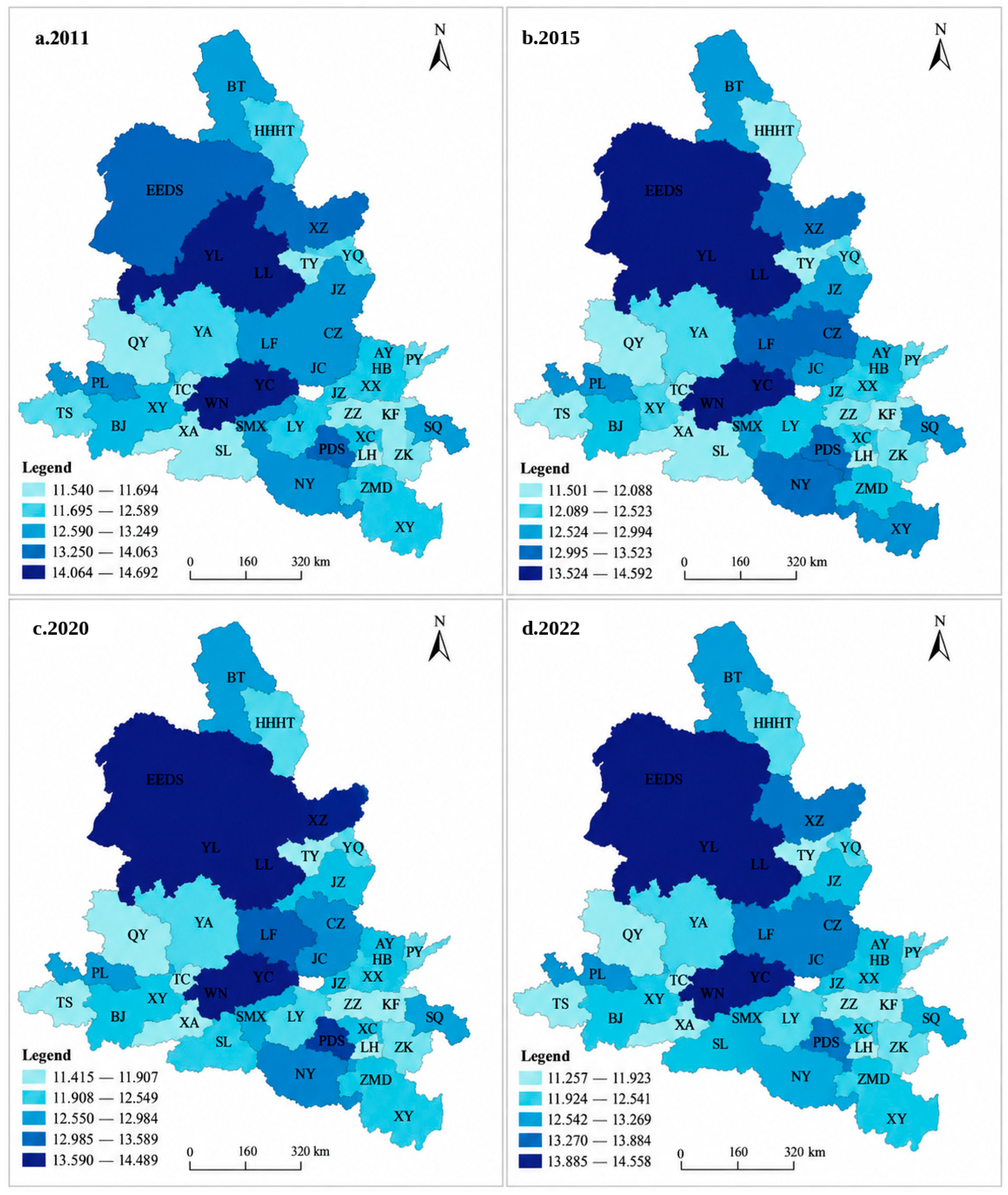
Figure 2 maps lnCLCI in 2011, 2015, 2020, and 2022. Because the class breaks are recalculated separately for each year, the color shades should be used to compare cities within the same map rather than to infer the magnitude of change from color differences across years. Figure 2 shows persistent spatial heterogeneity in lnCLCI, but the visual pattern is descriptive and does not by itself establish a policy spillover or transmission mechanism.

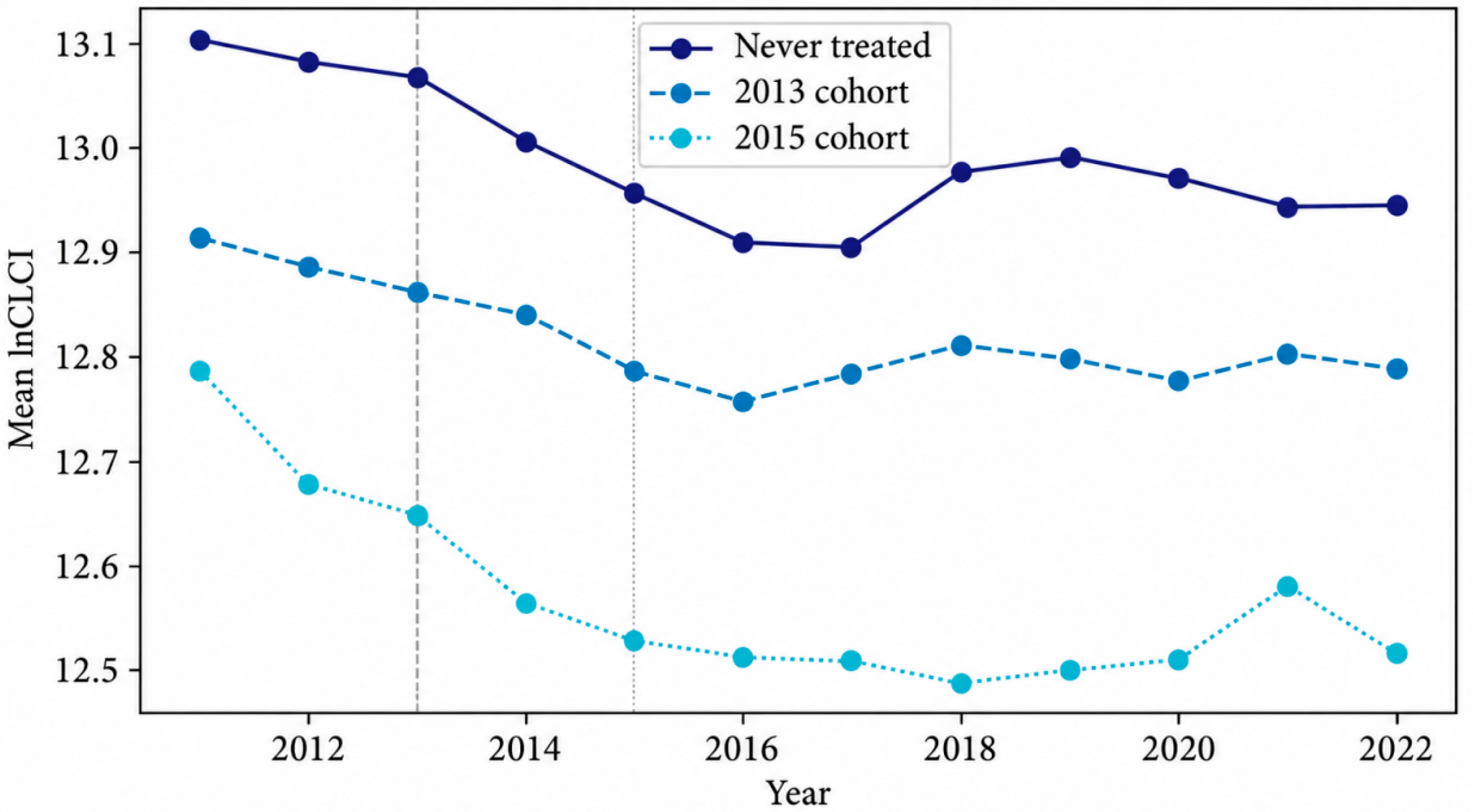
Figure 3 plots calendar-year mean lnCLCI for the 2013 treatment cohort, the 2015 treatment cohort, and the never-treated group. The three trajectories differ in their initial levels, and the 2015 cohort remains untreated until its adoption year. Figure 3 is therefore used only to describe cohort-level trajectories; it is not an event-study estimate or a treatment-effect plot. Relative-time policy dynamics are estimated separately in Figure 5.

4.4. Empirical Strategy

4.4.1. Group-Time Treatment Effects and TWFE Benchmark

The main policy analysis follows Callaway and Sant’Anna [38] and estimates ATT(g,t), the average treatment effect in year t for cities first treated in year g. Cities that were never treated serve as the comparison group. Identification requires no anticipation, absorbing treatment, comparable untreated trends, and sufficient covariate overlap between treated and comparison cities. The unadjusted specification compares changes in outcomes relative to the year before treatment, g−1. The adjusted specification uses the six covariates measured before treatment to model untreated outcome changes. Covariates are fixed at 2012 for the 2013 treatment cohort and at 2014 for the 2015 cohort, avoiding adjustment for variables that may themselves respond to the policy. Because the comparison group contains only 19 never-treated cities, covariate adjustment may require extrapolation where treated and comparison cities have limited overlap. The adjusted estimates are therefore interpreted with caution. Post-treatment ATT(g,t) estimates are aggregated across observed post-treatment periods using weights proportional to cohort size. Table 5 reports the overall and cohort-specific averages. Statistical inference is based on 999 city-cluster multiplier-bootstrap replications with seed 20261003. The Sun–Abraham event-study specification provides a separate check on treatment dynamics [41]. It uses never-treated cities as the control cohort, sets relative year −1 as the reference period, and is estimated without contemporaneous controls. The conventional TWFE model is retained as a conditional benchmark rather than the preferred estimator.

$$\ln \mathrm{C}\mathrm{L}\mathrm{C}{\mathrm{I}}_{\mathrm{i}\mathrm{t}}=\mathsf{\beta }\mathrm{S}\mathrm{C}{\mathrm{P}}_{\mathrm{i}\mathrm{t}}+{\mathsf{\gamma }}^{\prime }{\mathrm{X}}_{\mathrm{i}\mathrm{t}}+{\mathsf{\mu }}_{\mathrm{i}}+{\mathsf{\lambda }}_{\mathrm{t}}+{\mathsf{\epsilon }}_{\mathrm{i}\mathrm{t}}$$

Here, i indexes cities and t indexes years. SCP is the reconstructed treatment indicator, X contains the six benchmark controls, ${\mathsf{\mu }}_{\mathrm{i}}$ and ${\mathsf{\lambda }}_{\mathrm{t}}$ denote city and year fixed effects, and ${\mathsf{\epsilon }}_{\mathrm{i}\mathrm{t}}$ is the error term. TWFE standard errors are clustered at the city level using the CR1 covariance estimator with a finite-sample adjustment. Statistical inference uses the t distribution with 36 degrees of freedom for the 37 city clusters. This treatment of the standard errors allows for serial dependence within cities but does not account for dependence across cities. The group-time estimates likewise rely on the assumption that treatment in one city does not affect outcomes in another. Section 4.4.2 examines cross-city policy exposure separately rather than treating the spatial analysis as a correction for this assumption.

Table 5. DID estimates under alternative treatment definitions and staggered adoption.

Estimator or Sample	Estimate	SE	p-Value	95% Interval
Group-time ATT, unadjusted	0.026	0.072	0.708	−0.117 to 0.170
Group-time ATT, pre-treatment covariates	−0.040	0.098	0.673	−0.226 to 0.145
TWFE, strict 37-city sample	0.008	0.069	0.909	−0.132 to 0.148
TWFE, strict all-city coding	0.019	0.065	0.772	−0.113 to 0.151
TWFE, broad all-city coding	−0.013	0.065	0.848	−0.144 to 0.119
2013 cohort, unadjusted	0.031	0.085	0.716	−0.125 to 0.188
2015 cohort, unadjusted	0.010	0.115	0.933	−0.193 to 0.213

Note: Group-time estimates use never-treated cities and 999 city-cluster multiplier-bootstrap replications. TWFE estimates include city and year effects, with city-clustered CR1 inference. The preferred sample has 444 observations and 37 cities; the all-city samples have 480 observations. Table 5 reports overall and cohort aggregates. Event-study intervals are pointwise rather than simultaneous bands.

Table 5. DID estimates under alternative treatment definitions and staggered adoption.

Estimator or Sample	Estimate	SE	p-Value	95% Interval
Group-time ATT, unadjusted	0.026	0.072	0.708	−0.117 to 0.170
Group-time ATT, pre-treatment covariates	−0.040	0.098	0.673	−0.226 to 0.145
TWFE, strict 37-city sample	0.008	0.069	0.909	−0.132 to 0.148
TWFE, strict all-city coding	0.019	0.065	0.772	−0.113 to 0.151
TWFE, broad all-city coding	−0.013	0.065	0.848	−0.144 to 0.119
2013 cohort, unadjusted	0.031	0.085	0.716	−0.125 to 0.188
2015 cohort, unadjusted	0.010	0.115	0.933	−0.193 to 0.213

Note: Group-time estimates use never-treated cities and 999 city-cluster multiplier-bootstrap replications. TWFE estimates include city and year effects, with city-clustered CR1 inference. The preferred sample has 444 observations and 37 cities; the all-city samples have 480 observations. Table 5 reports overall and cohort aggregates. Event-study intervals are pointwise rather than simultaneous bands.

Selection adjustment is used only as a supplementary check. Matching is based on city averages of the six benchmark controls over 2011–2012. Propensity scores are estimated with a standardized logistic model using an L2 penalty with C = 1, followed by one-to-one nearest-neighbor matching with replacement and no caliper. The matched regression includes city and year fixed effects, while the reported covariance treats the estimated matches as fixed. Entropy balancing uses the same six pre-policy covariate means and seeks exact balance through nonnegative weights assigned to comparison cities. A linear programming support check shows that the treated-group covariate target lies outside the feasible convex support of the comparison group. Exact entropy balance is therefore not feasible in this sample, and no entropy-balancing policy coefficient is reported.

Figure 2. Spatial distribution of log built-up land carbon intensity (lnCLCI), 2011, 2015, 2020, and 2022.

Figure 2. Spatial distribution of log built-up land carbon intensity (lnCLCI), 2011, 2015, 2020, and 2022.

4.4.2. Spatial Policy Exposure Specification

The spatial analysis examines whether policy exposure in other cities is associated with lnCLCI after local Smart City Pilot treatment is controlled. The main specification uses an inverse geographic distance matrix with zero diagonal elements and row-standardized weights. Contiguity is the alternative geographic specification; the archived ratio network is retained only as a diagnostic. Neighboring policy exposure is defined as follows:

$$\mathrm{W}\mathrm{S}\mathrm{C}{\mathrm{P}}_{\mathrm{i}\mathrm{t}}={\sum }_{\mathrm{j}\ne \mathrm{i}}{\mathrm{w}}_{\mathrm{i}\mathrm{j}}\mathrm{S}\mathrm{C}{\mathrm{P}}_{\mathrm{j}\mathrm{t}}$$

w denotes a fixed spatial-weight matrix with zeros on the diagonal. The main geographic specification uses inverse distance, reflecting the assumption that cross-city policy exposure weakens as geographic separation increases. A contiguity matrix is used as a discrete alternative and assigns exposure only between cities that share a common boundary. Both matrices are matched by numeric city ID, restricted to the 37-city policy sample, and row-normalized after the sample exclusions. Rows with no neighbors remain zero. The archived Wgdp1 matrix is used only as a diagnostic specification. Its raw element is defined as ${\displaystyle \frac{{\mathrm{q}}_{\mathrm{i}}}{{\mathrm{q}}_{\mathrm{j}}}}$, where ${\mathrm{q}}_{\mathrm{i}}$ is the 2011–2022 city average of resident population divided by GDP after applying the unit conversions recorded in the archive. This construction represents a ratio of full-period inverse-income measures rather than a pairwise measure of economic distance. It also incorporates information from post-treatment years. For these reasons, Wgdp1 is not interpreted as a pre-policy economic network and is not used as a robustness test based on economic distance.

Figure 3. Annual mean lnCLCI by strict whole-city treatment cohort and never-treated status. (Note: The vertical gray reference lines indicate the policy adoption years for the 2013 and 2015 treatment cohorts respectively).

Figure 3. Annual mean lnCLCI by strict whole-city treatment cohort and never-treated status. (Note: The vertical gray reference lines indicate the policy adoption years for the 2013 and 2015 treatment cohorts respectively).

The spatial-exposure regression is specified as

$$\ln \mathrm{C}\mathrm{L}\mathrm{C}{\mathrm{I}}_{\mathrm{i}\mathrm{t}}=\mathsf{\beta }\mathrm{S}\mathrm{C}{\mathrm{P}}_{\mathrm{i}\mathrm{t}}+\mathsf{\theta }{\sum }_{\mathrm{j}\ne \mathrm{i}}{\mathrm{w}}_{\mathrm{i}\mathrm{j}}\mathrm{S}\mathrm{C}{\mathrm{P}}_{\mathrm{j}\mathrm{t}}+\mathsf{\gamma }\prime {\mathrm{X}}_{\mathrm{i}\mathrm{t}}+\mathsf{\eta }\prime {\sum }_{\mathrm{j}\ne \mathrm{i}}{\mathrm{w}}_{\mathrm{i}\mathrm{j}}{\mathrm{X}}_{\mathrm{j}\mathrm{t}}+{\mathsf{\mu }}_{\mathrm{i}}+{\mathsf{\lambda }}_{\mathrm{t}}+{\mathsf{\epsilon }}_{\mathrm{i}\mathrm{t}}$$

Here, i and j index cities and t indexes years; ${\mathrm{w}}_{\mathrm{i}\mathrm{j}}$ is the normalized spatial weight linking city j to city i, with ${\mathrm{w}}_{\mathrm{i}\mathrm{i}}=0$. $\mathrm{S}\mathrm{C}{\mathrm{P}}_{\mathrm{i}\mathrm{t}}$ is the local Smart City Pilot treatment indicator, while $\mathrm{S}\mathrm{C}{\mathrm{P}}_{\mathrm{j}\mathrm{t}}$ denotes the treatment status of city j used to construct neighboring policy exposure. ${\mathrm{X}}_{\mathrm{i}\mathrm{t}}$ contains the six benchmark control variables, and ${\mathrm{X}}_{\mathrm{j}\mathrm{t}}$ contains the corresponding controls for city j. The spatially weighted terms capture policy exposure and observed characteristics in other cities according to the specified spatial weight matrix. City fixed effects are denoted by ${\mathsf{\mu }}_{\mathrm{i}}$, year fixed effects by ${\mathsf{\lambda }}_{\mathrm{t}}$, and ${\mathsf{\epsilon }}_{\mathrm{i}\mathrm{t}}$ is the error term. The coefficient $\mathsf{\beta }$ measures the conditional association between local pilot designation and lnCLCI, while $\mathsf{\theta }$ captures the conditional association with neighboring policy exposure. The vectors $\mathsf{\gamma }$ and $\mathsf{\eta }$ are the coefficient vectors for the local and spatially weighted control variables, respectively. The specification does not include a spatial lag of the dependent variable. Standard errors are estimated using city-clustered CR1 covariance with 36 degrees of freedom. This adjustment allows for within-city dependence over time but does not account for residual dependence across cities. The coefficients $\mathsf{\beta }$ and $\mathsf{\theta }$ are therefore interpreted as conditional associations rather than fully identified direct and spillover treatment effects.

4.4.3. Related Outcomes and Pre-Policy Heterogeneity

Related-outcome regressions use the same sample, controls, and city and year fixed effects as the TWFE benchmark. The outcomes include energy intensity, log GDP per unit of built-up land, log resident population per unit of built-up land, and annual built-up land growth. These regressions are used to examine related policy responses rather than mediation. The land-based outcomes either share the built-up land denominator with lnCLCI or are constructed directly from BUA. DII and INS are excluded due to the data limitations described in Section 4.2. Heterogeneity is examined using groups defined before treatment. Population-density groups are based on each city’s mean log administrative population density over 2011–2012, while land-growth groups use the mean built-up land growth rate over the same period.

For each variable, cities above the median of the preferred sample are assigned to the high group. Differences between groups are tested in a pooled model using the interaction between SCP and the fixed group indicator. The SCP coefficient represents the estimated effect for the low group, while the sum of the SCP and interaction coefficients gives the estimated effect for the high group. Whether the two groups differ is assessed from the interaction coefficient itself rather than from separate significance tests within each subgroup.

4.4.4. Predictive Machine Learning Analysis

The prediction sample covers all 40 cities from 2013 to 2022, excluding the two backcast DII years. Candidate predictors include SCP, DII, energy intensity, and the six benchmark controls. INS is excluded because its construction is not documented. Training and test samples are split by city rather than by individual observations. With seed 42, 32 cities are used for model training and eight cities are held out for evaluation. Five-fold GroupKFold is applied within the training sample, with cities kept intact across folds. Recursive feature elimination with cross-validation (RFECV) removes one predictor at a time according to cross-validated R², and feature selection is based only on the training data. The Random Forest contains 100 trees, uses squared-error splitting, places no restriction on tree depth, and retains the default minimum leaf size. No hyperparameter search is conducted. An OLS model using all nine candidate predictors is evaluated on the same held-out cities to provide a common benchmark. The implementation sorts observations by city ID and year and passes predictors in the order SCP, EI, DII, lninvest, lnauthorizations, lnGDP, lndens, fiscal, urban. GroupShuffleSplit uses a test fraction of 0.20. Forest and split random states use the corresponding reported seed. Other forest settings are min_samples_split = 2, min_samples_leaf = 1, max_features = 1.0, and bootstrap = True.

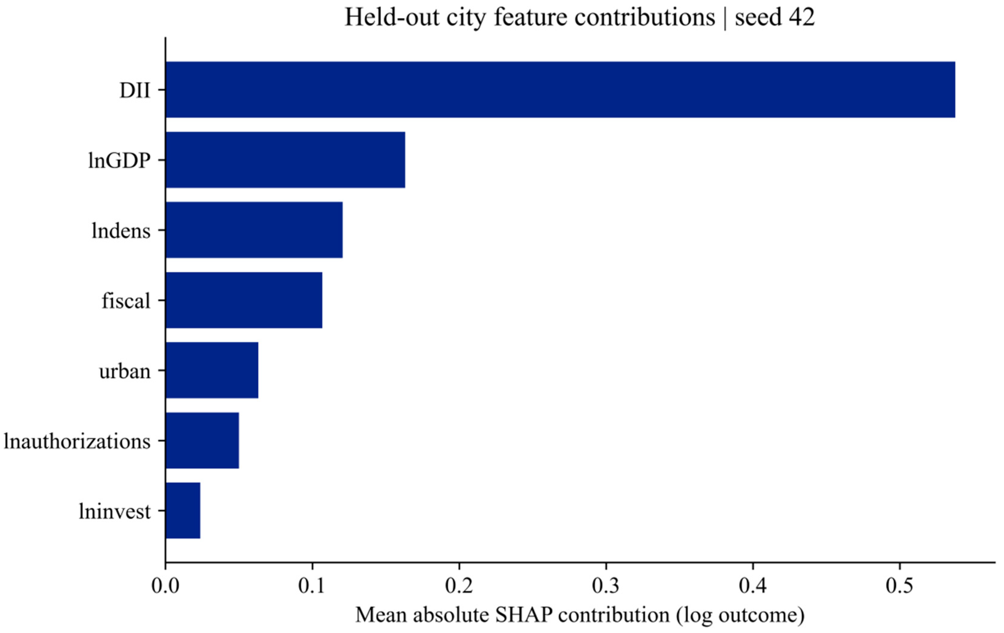
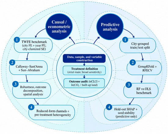
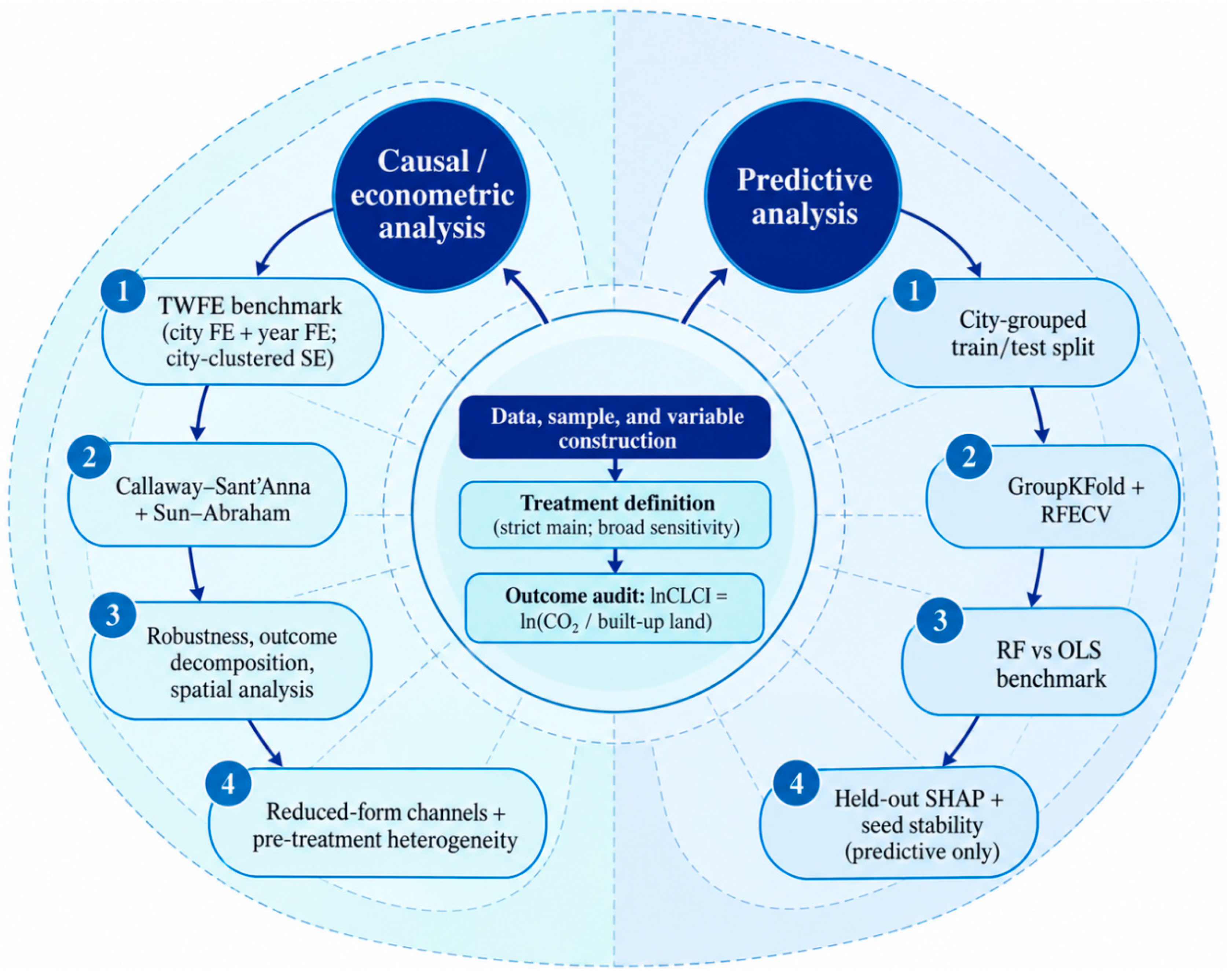
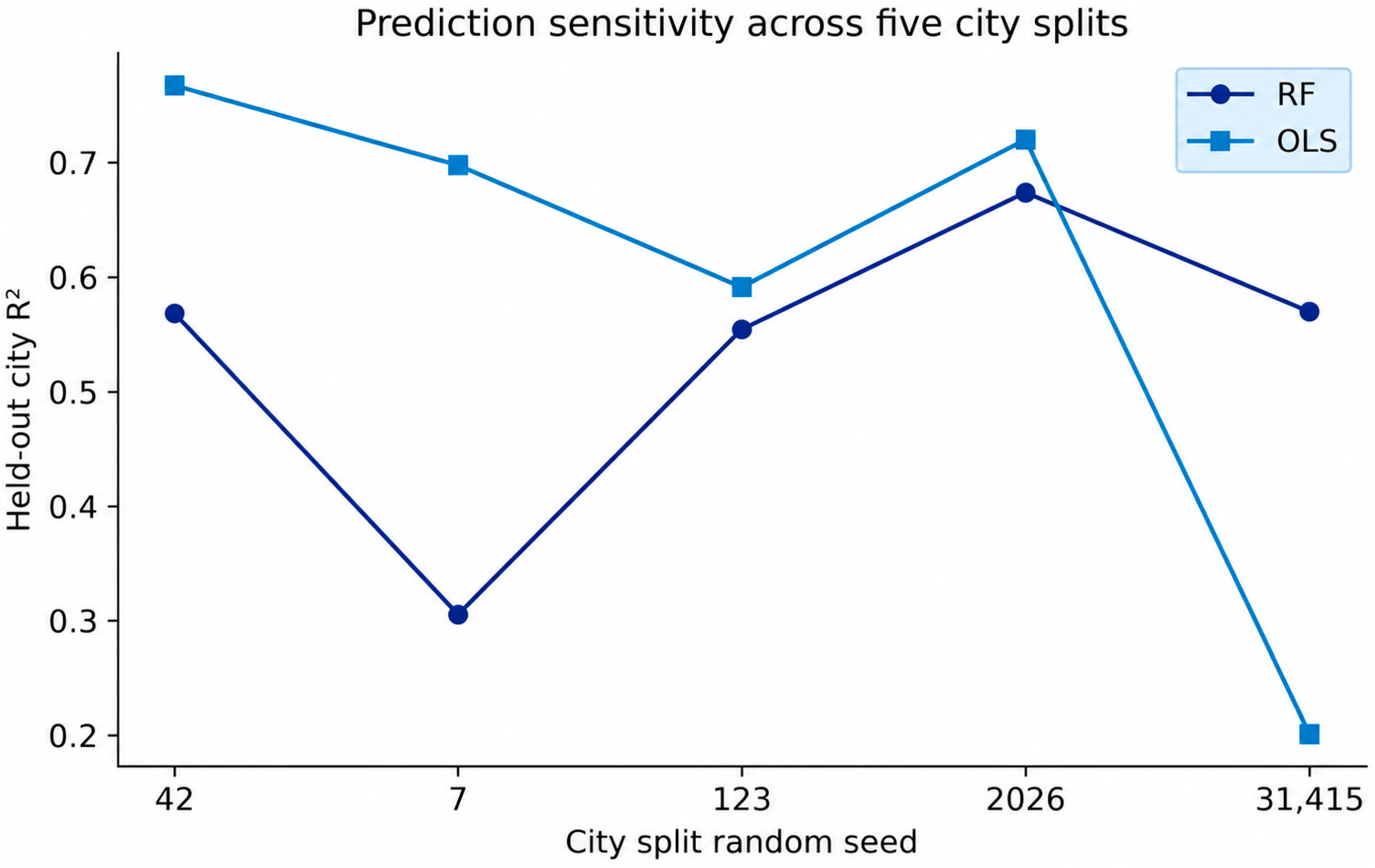
The full grouped procedure is repeated with seeds 7, 123, 2026, and 31415 to assess sensitivity to the particular cities held out for testing. Figure 6 reports held-out R² for Random Forest and OLS across the five city splits. For the seed-42 Random Forest, SHAP values are calculated only for observations from the held-out cities. Mean absolute SHAP values summarize how strongly each predictor contributes to the model’s predictions in that test sample. Because DII may itself respond to SCP, its predictive importance is not interpreted as evidence of a policy channel or mediation effect. The analysis measures contemporaneous prediction across cities rather than forecasting future outcomes. Post-selection cross-validation is reported only as an internal diagnostic because the same training folds also contribute to feature selection. Figure 4 summarizes this analytical sequence and keeps policy estimation, supporting diagnostics, and city-grouped prediction as separate tasks.

Figure 4. Analytical workflow separating policy estimation, supporting diagnostics, and city-grouped prediction.

5. Empirical Results

5.1. Main Policy Estimates

As reported in Table 5, the unadjusted group-time ATT is 0.026, with a standard error of 0.072 and a p-value of 0.708. After adjustment for pre-treatment covariates, the estimate changes to −0.040, with a standard error of 0.098 and a p-value of 0.673. The confidence intervals for both estimates include zero. The TWFE benchmark in Table 5 is similarly small at 0.008, with a standard error of 0.069 and a p-value of 0.909; its 95% confidence interval ranges from −0.132 to 0.148. Taken together, the estimates in Table 5 do not provide evidence that Smart City Pilot designation reduced lnCLCI on average, and H1 is therefore not supported. The intervals are also too wide to conclude that the underlying policy effect is exactly zero.

The treatment-scope checks in Table 5 lead to the same conclusion. Using the strict treatment definition in the full 40-city sample gives a TWFE coefficient of 0.019, with a p-value of 0.772, while assigning the three sub-prefectural pilots to their parent cities gives a coefficient of −0.013, with a p-value of 0.848. Neither specification provides evidence of an average decline in lnCLCI. Given the uncertainty around these estimates, the benchmark coefficient is not translated into a percentage policy effect.

5.2. Dynamic Effects: Pre-Policy Trends and Post-Policy Changes

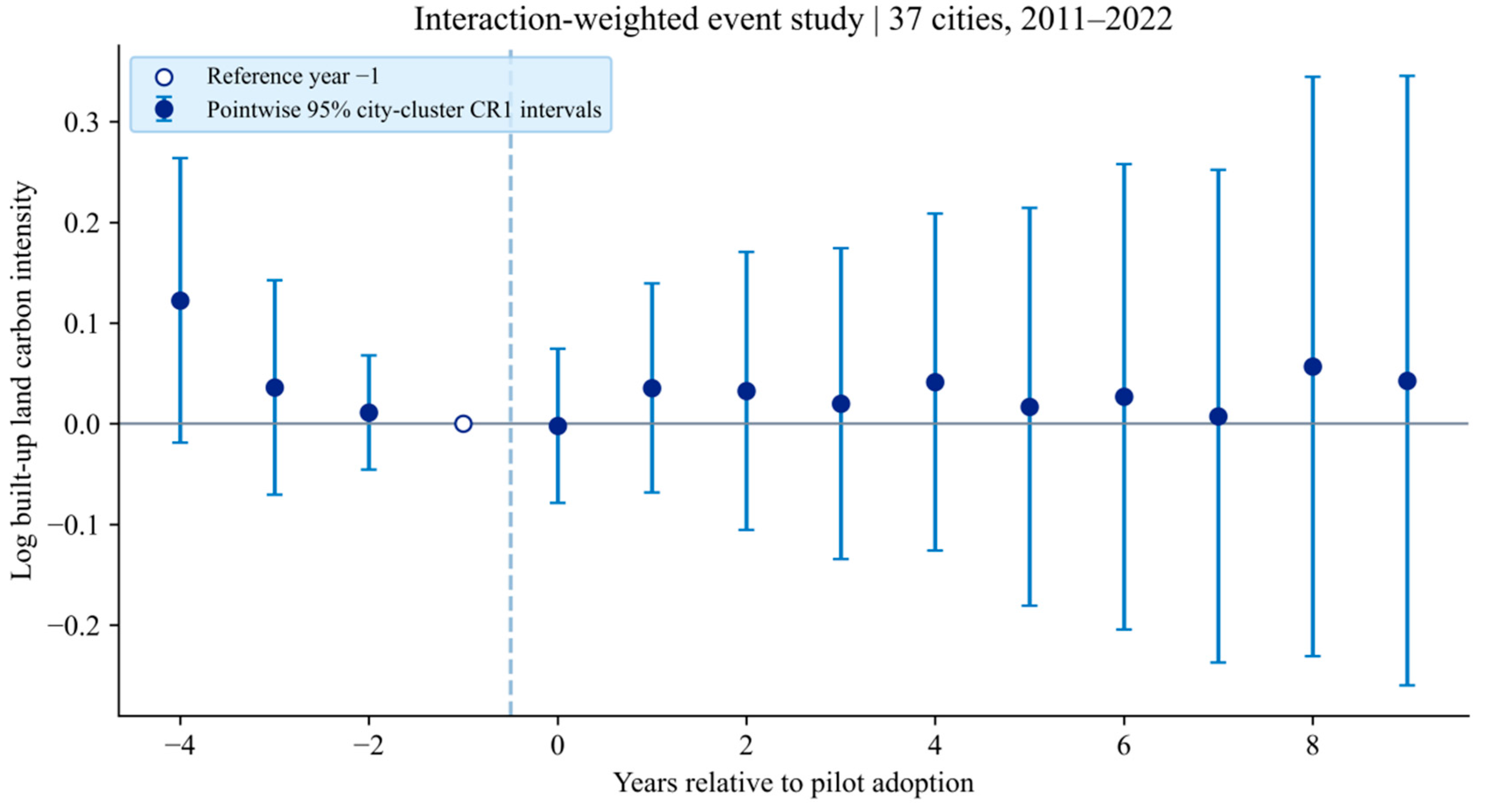
Figure 5 presents the Sun–Abraham event-time estimates. The pointwise confidence intervals include zero in all pre-treatment and post-treatment periods. Relative years −4 and −3 are identified only by the 2015 cohort, both cohorts contribute to estimates from relative year −2 through 7, and years 8 and 9 are identified only by the 2013 cohort. Because the common pre-treatment window is short, the non-significant lead coefficients provide only limited evidence on the parallel-trends assumption. The composition of the contributing cohorts also changes across event time, so the estimated profile should not be read as the path of a fixed group of cities.

The post-treatment coefficients show no sustained decline in lnCLCI. Table 5 reports the cohort-level average effects, while Figure 5 reports period-specific event-time dynamics.

Figure 5. Sun–Abraham interaction-weighted event-time estimates with city-clustered pointwise 95% confidence intervals; relative year −1 is the reference period. (Note: The vertical blue dashed line marks the boundary between the pre-treatment and post-treatment periods, with treatment beginning at relative year 0).

Figure 5. Sun–Abraham interaction-weighted event-time estimates with city-clustered pointwise 95% confidence intervals; relative year −1 is the reference period. (Note: The vertical blue dashed line marks the boundary between the pre-treatment and post-treatment periods, with treatment beginning at relative year 0).

5.3. Outcome and Design Sensitivity

5.3.1. Emissions and Land-Area Decomposition

The ratio decomposition estimates lnCO₂ and lnBUA using the same 37-city sample, benchmark controls, and city and year fixed effects as the main TWFE specification. Using a common specification keeps the two component regressions directly comparable with the decomposition of lnCLCI. Controls for concurrent policies and selection-adjustment results are reported separately because they address different sources of potential bias and are not part of the accounting decomposition itself.

Table 6 shows that the estimated coefficient for lnCO₂ is −0.042, with a standard error of 0.047 and a p-value of 0.382, while the coefficient for lnBUA is −0.050, with a standard error of 0.049 and a p-value of 0.316. Their difference reproduces the lnCLCI coefficient to numerical precision, as required by the accounting identity lnCLCI = lnCO₂ − lnBUA under the common sample and specification. The confidence intervals in Table 6 include zero for both components, so the estimates do not determine whether the small lnCLCI response reflects lower emissions, a change in built-up land area, or a combination of both.

Table 6. Policy responses in the ratio and its components.

Outcome	Estimate	SE	p-Value	95% Interval
lnCLCI	0.008	0.069	0.909	−0.132 to 0.148
lnCO2	−0.042	0.047	0.382	−0.138 to 0.054
lnBUA	−0.050	0.049	0.316	−0.149 to 0.050

Note: All component regressions use the preferred 37-city sample and the same TWFE specification. The coefficient identity follows from lnCLCI = lnCO₂ − lnBUA when the sample and regressors are identical.

5.3.2. Concurrent Policies

As shown in Table 7, adding the low-carbon city, Broadband China, and innovative-city indicators separately leaves the SCP coefficient close to zero and statistically imprecise in each specification. The estimates range from 0.004 to 0.019, and all reported confidence intervals include zero. Table 7 therefore indicates that the benchmark conclusion is not materially changed by these observed policy-overlap controls, although the exercise cannot remove unmeasured interactions among programs.

Table 7. Benchmark estimates with concurrent policy controls.

Additional Policy	SCP Estimate	SE	p-Value	95% Interval
Low-carbon city pilot	0.004	0.071	0.950	−0.139 to 0.148
Broadband China	0.019	0.069	0.786	−0.121 to 0.158
Innovative city pilot	0.016	0.070	0.825	−0.127 to 0.158

Note: Each policy is added separately. Indicators are rebuilt from valid adoption years on the city matching sheet. A policy year of zero denotes no treatment. The province-level low-carbon designation is time-invariant within the observed sample and is absorbed by city fixed effects; the regional emissions-trading pilot indicator has no qualifying treated city in this sample.

5.3.3. Selection Adjustment Using Pre-Policy Covariates

Table 8 reports the selection-adjusted TWFE estimate after city-level nearest-neighbor matching on pre-policy covariates. The estimated SCP coefficient is −0.081, with a standard error of 0.108 and a p-value of 0.458, so the matched estimate remains statistically imprecise.

Table 8. Selection-adjusted TWFE estimates.

Estimator	SCP Estimate	SE	p-Value	95% Interval
City-level nearest-neighbor matching	−0.081	0.108	0.458	−0.302 to 0.140

Note: Matching uses city means of the six controls over 2011–2012, a standardized covariate logistic propensity model with L2 penalty C = 1, and one nearest control per treated city, with replacement and no caliper. It yields 27 distinct cities and 324 observations. Control multiplicities determine weights. The weighted regression includes city and year fixed effects and city-clustered CR1 inference over 26 degrees of freedom; inference conditions on estimated weights and does not account for matching uncertainty. Exact mean entropy balancing on the same six pre-policy controls is infeasible under nonnegative control weights, as verified by a linear programming support check. No entropy-balancing coefficient is reported.

The matching procedure underlying Table 8 improves balance on observed pre-treatment characteristics, but it does not impose a caliper and may therefore retain relatively distant matches. The reported covariance also treats the estimated matches as fixed. Exact entropy balancing with nonnegative weights is not feasible because the treated-group covariate means lie outside the convex support of the comparison cities. These procedures address observed selection only. They do not resolve staggered treatment heterogeneity, unobserved selection, overlapping policies, or possible cross-city interference.

Across these design checks, the estimated policy effects remain statistically imprecise. The results are therefore interpreted based on the magnitude of the estimates and their uncertainty rather than from individual p-values alone.

5.4. Spatial Policy Exposure

Table 9 shows that the coefficients on W × SCP are statistically imprecise under both the inverse-distance and adjacency matrices. The archived ratio-network specification produces a much larger coefficient, but this matrix is neither a pairwise distance measure nor predetermined because it is constructed from full-period inverse-income information. The corresponding rows in Table 9 are therefore reported only as a diagnostic. More generally, a coefficient on W × SCP cannot distinguish whether a cross-city association reflects policy learning, technology diffusion, industrial relocation, or another process.

Table 9. Conditional policy exposure under alternative spatial matrices.

Matrix and Term	Estimate	SE	p-Value	95% Interval
Inverse distance local SCP	−0.064	0.056	0.264	−0.178 to 0.050
Inverse distance W × SCP	−0.559	0.774	0.475	−2.128 to 1.010
Adjacency local SCP	−0.004	0.048	0.932	−0.101 to 0.093
Adjacency W × SCP	0.073	0.130	0.576	−0.190 to 0.336
Archived ratio diagnostic local SCP	−0.213	0.104	0.048	−0.424 to −0.002
Archived ratio diagnostic W × SCP	−7.745	2.595	0.005	−13.007 to −2.482

Note: Table 9 reports coefficients from the linear spatial-exposure model in Section 4.4.2. Each specification includes weighted controls, city and year fixed effects, and city-clustered CR1 inference. Matrices are restricted to the 37-city sample and row-normalized after exclusions. The archived ratio network uses full-period inverse-income information and is shown only as a diagnostic, not as an economic-distance robustness specification.

The spatial results are sensitive to how inter-city connections are defined, and neither geographic matrix provides clear evidence of a cross-city policy effect. H2 is therefore not supported by a result that is stable across network definitions. Because dependence in regression residuals across cities is not explicitly modeled, the estimates in Table 9 are interpreted as conditional associations rather than separate causal spillover effects.

5.5. Related Outcomes and Channel Limitations

As reported in Table 10, the estimated coefficient for energy intensity is 0.002, with a standard error of 0.013 and a p-value of 0.892. The coefficient for lnGDPperBUA is 0.050 (SE = 0.049, p = 0.316), while the coefficient for lnpopBUA is 0.047 (SE = 0.050, p = 0.348). These estimates provide no clear evidence that the policy changed energy intensity, land-based economic output, or population accommodated per unit of built-up land. Table 10 also reports an annual built-up land growth coefficient of −0.042, with a standard error of 0.021 and a p-value of 0.054. This estimate is consistent with slower land expansion in treated cities, but its 95% interval still includes zero. Moreover, land growth, lnGDPperBUA, and lnpopBUA are all constructed from BUA, so their signs cannot be treated as independent evidence of a mechanism behind changes in lnCLCI.

Table 10. Related-outcome regressions.

Outcome	SCP Estimate	SE	p-Value	95% Interval
EI	0.002	0.013	0.892	−0.025 to 0.028
lnGDPperBUA	0.050	0.049	0.316	−0.050 to 0.149
lnpopBUA	0.047	0.050	0.348	−0.053 to 0.148
land_expand	−0.042	0.021	0.054	−0.086 to 0.001

Note: Table 10 uses the TWFE benchmark specification. lnpopBUA is reconstructed from resident population and built-up area. The archived land_POP series is not used because it does not measure resident population per unit of built-up land. Since lnGDP is already a control, the coefficient on lnGDPperBUA is mechanically the negative of the lnBUA coefficient under this specification and provides no independent channel evidence. lnpopBUA and land_expand are also denominator-related outcomes, not mediation estimates.

DII is excluded because observed pre-policy values are unavailable for the first treatment cohort, while INS is excluded because its original construction cannot be recovered from the archived materials. The archived land_POP variable is also not used. It equals administrative population density divided by built-up land area and by ten, rather than resident population per unit of built-up land. Table 10 instead reports lnpopBUA reconstructed directly from resident population and BUA. These data limitations mean that H3a cannot be tested for the first cohort using observed pre-policy DII. The remaining related-outcome regressions also do not establish H3b or H3c as causal channels.

A policy coefficient for a related outcome, even if estimated precisely, would not by itself identify mediation. Establishing an indirect effect would require a separate mediation design, particularly when the proposed channel shares the BUA denominator with lnCLCI or may itself respond to treatment.

5.6. Heterogeneity Using Pre-Policy City Conditions

As shown in Table 11, the high-minus-low density difference is −0.123, with a standard error of 0.090 and a p-value of 0.180. For pre-policy land expansion, the corresponding difference is 0.059, with a standard error of 0.087 and a p-value of 0.498. Neither interaction provides clear evidence that the SCP effect differs between the two groups. Table 11 evaluates heterogeneity from the pooled interaction coefficient and its uncertainty rather than from separate significance tests within each subgroup. The results therefore do not support H4 in this sample, and the density interaction is too imprecise to justify a policy recommendation based on population density.

Table 11. Pooled interaction tests with pre-policy groups.

Pre-Policy Dimension and Contrast	Estimate	SE	p-Value	95% Interval
lndens low	0.066	0.083	0.431	−0.103 to 0.235
lndens high	−0.057	0.076	0.461	−0.211 to 0.098
lndens difference	−0.123	0.090	0.180	−0.305 to 0.059
land_expand low	−0.028	0.064	0.662	−0.158 to 0.101
land_expand high	0.031	0.090	0.731	−0.152 to 0.214
land_expand difference	0.059	0.087	0.498	−0.117 to 0.235

Note: Groups use 2011–2012 city means and the preferred-sample median. High-group values exceed that median. Low and high effects are linear combinations from the same pooled interaction model; the interaction tests their difference. All models include the six controls and city and year effects.

5.7. Prediction in Held-Out Cities

The machine learning analysis predicts lnCLCI for cities that are excluded from model fitting, using all 40 cities observed from 2013 to 2022. It is designed to assess cross-city predictive performance rather than to estimate a policy counterfactual. Predictive accuracy and feature contributions are therefore reported separately from the treatment-effect results.

5.7.1. Predictive Performance and Feature Selection

Table 12 reports that, for the seed-42 split, Random Forest achieves a held-out-city R² of 0.568, with an RMSE of 0.400 and an MAE of 0.328. The OLS benchmark performs better on the same held-out cities, with an R² of 0.767, an RMSE of 0.294, and an MAE of 0.251. Within the training sample, Table 12 also shows a mean cross-validated R² of −0.040 for Random Forest, with a standard deviation of 1.075, indicating substantial variation across city folds.

Table 12. Predictive performance under city-grouped validation.

Model	Test R2	Test RMSE	Test MAE	CV Mean R2	CV SD
Random Forest	0.568	0.400	0.328	−0.040	1.075
OLS benchmark	0.767	0.294	0.251	−0.124	1.319

Note: Seed 42 assigns 32 cities (320 observations) to training and eight cities (80 observations) to testing. Five-fold GroupKFold uses training cities only, and feature selection is confined to the training sample. Cross-validation values are post-selection diagnostics; test metrics come from held-out cities. The OLS benchmark includes all nine candidate predictors.

Figure 6 shows the sensitivity of held-out-city R² to the city split. Across the five random seeds, Random Forest ranges from 0.305 to 0.673, while OLS ranges from 0.201 to 0.767. The relative ranking changes across splits, indicating that predictive performance depends materially on which cities are held out.

Figure 6. Prediction sensitivity across five city-grouped train; held-out-city R² for Random Forest and OLS.

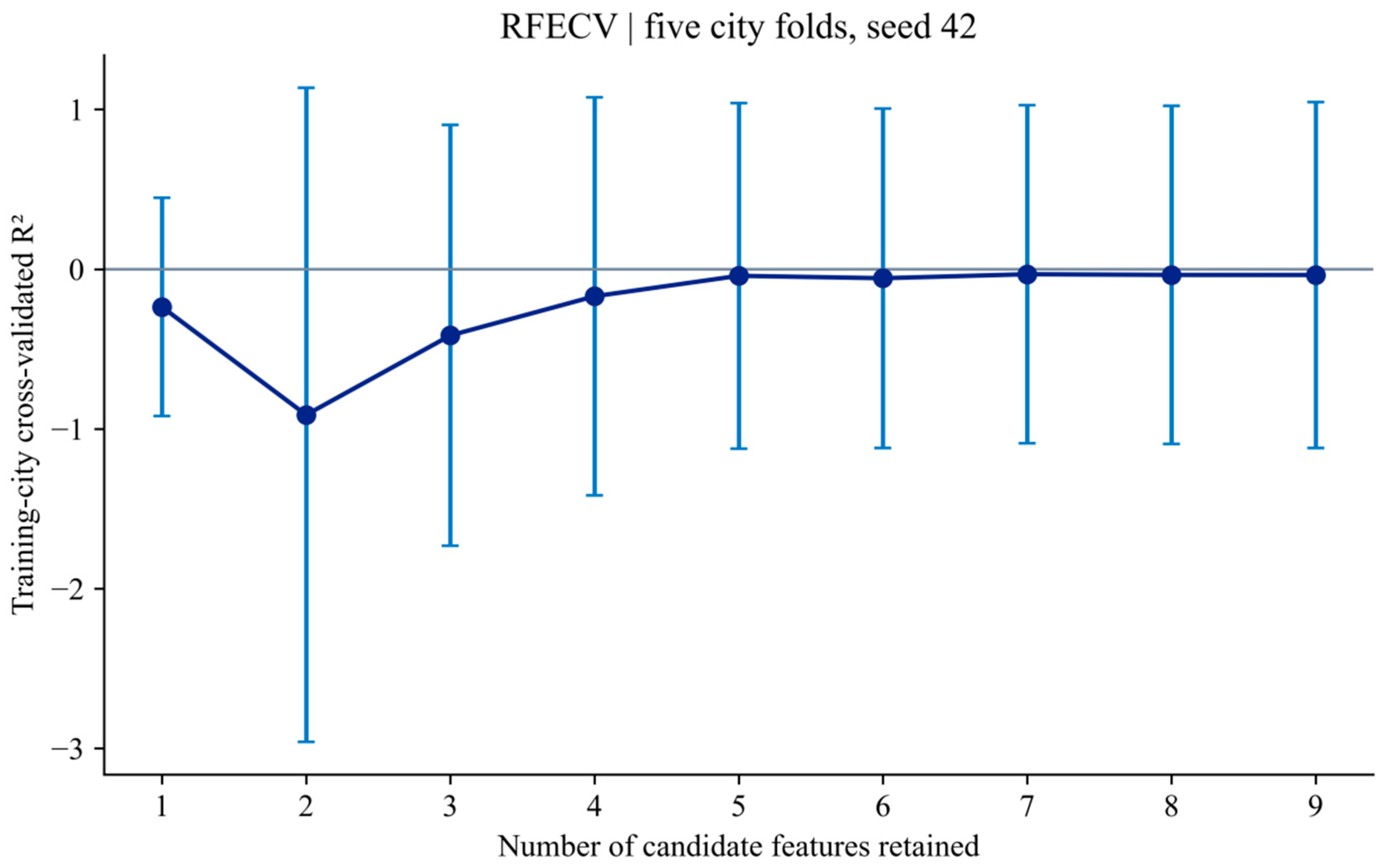
Figure 7 complements Table 12 by showing the RFECV training-city cross-validation profile over one to nine candidate features. The fold scores vary substantially, and RFECV retains seven predictors in the seed-42 specification: DII and the six benchmark controls. SCP and EI are not selected in this split. Selection or exclusion of SCP is not evidence of a causal policy effect.

5.7.2. Feature Contributions

Table 13 reports the retained predictors and their Random Forest importance and mean absolute SHAP values for the seed-42 model, while Figure 8 visualizes the held-out-city ranking. DII has the largest mean absolute SHAP value at 0.538, followed by lnGDP at 0.163, lndens at 0.121, and fiscal at 0.107. SCP and EI are not retained, so no SHAP contribution is estimated for them in this selected forest. These quantities describe contributions to prediction; because predictors are correlated and DII may itself respond to SCP, neither Table 13 nor Figure 8 is interpreted as evidence of mediation or a policy mechanism.

Table 13. Feature contributions in the Seed-42 Forest.

Feature	Retained	RF Importance	Mean |SHAP|
DII	Yes	0.5879	0.5378
lnGDP	Yes	0.0835	0.1633
lndens	Yes	0.0958	0.1207
fiscal	Yes	0.0988	0.1069
urban	Yes	0.0465	0.0633
lnauthorizations	Yes	0.0512	0.0500
lninvest	Yes	0.0363	0.0238
EI	No	—	—
SCP	No	—	—

Note: Random Forest importance is based on training-tree impurity reductions. Mean absolute SHAP values use held-out observations. An excluded predictor has no contribution estimate in the selected model; it is not assigned a measured causal or predictive effect of zero.

Figure 7. RFECV performance using training-city GroupKFold; error bars show one standard deviation across folds. (Note: The blue line and markers show the mean cross-validated R²; the vertical error bars indicate one standard deviation across folds; the gray horizontal line denotes the R² = 0 reference level).

Figure 7. RFECV performance using training-city GroupKFold; error bars show one standard deviation across folds. (Note: The blue line and markers show the mean cross-validated R²; the vertical error bars indicate one standard deviation across folds; the gray horizontal line denotes the R² = 0 reference level).

The SHAP analysis is also not used to define a policy threshold. Identifying a causal cutoff would require a separate research design and evidence that the threshold is stable across samples and specifications. The reported SHAP results are therefore limited to describing feature contributions in the held-out-city predictions.

5.7.3. Scope of Predictive Interpretation

The prediction analysis can be reproduced from the archived analytical inputs, although the upstream emissions boundary and the original construction of DII are not fully documented. Splitting the data by city ensures that no city appears in both the training and test samples. This design reduces leakage across cities but does not remove uncertainty in the source data or convert contemporaneous prediction into forecasting.

Prediction performance is evaluated using held-out errors and variation across city splits, while SHAP is used to describe how the fitted model generates its predictions. Neither the prediction metrics nor the SHAP results are interpreted as evidence of mediation, causal interaction, or a policy threshold.

Figure 8. Mean absolute SHAP contributions for held-out cities in the seed-42 model.

Figure 8. Mean absolute SHAP contributions for held-out cities in the seed-42 model.

6. Discussion

6.1. The Policy Result and the Land-Based Outcome

The main estimates in Table 5 provide no clear evidence that Smart City Pilot designation reduced lnCLCI on average. The unadjusted ATT is 0.026, the estimate adjusted for pre-treatment covariates is −0.040, and the TWFE coefficient is 0.008. All three estimates are imprecise, leaving both modest positive and modest negative effects compatible with the data. This finding applies to lnCLCI in the regional sample studied here and should not be extended to other environmental outcomes or policy settings.

lnCLCI measures city carbon emissions relative to built-up land area. It is neither a measure of carbon productivity nor a substitute for total emissions [69,70,71,72]. A city may improve carbon performance relative to economic output while continuing to expand developed land. It may also record lower emissions per unit of built-up land even when total emissions do not fall. Interpretation therefore depends on changes in both emissions and BUA, as well as on whether the two measures refer to compatible spatial boundaries.

The component results in Table 6 do not show a clear policy response in either lnCO₂ or lnBUA. Reporting both components is important because a change in their ratio cannot be interpreted automatically as a reduction in absolute emissions. The related-outcome results in Table 10 face a similar limitation: several land-based measures share BUA as a denominator, while incomplete source documentation prevents a verified mediation analysis. A low lnCLCI value alone therefore does not establish efficient land use or successful decarbonization. It needs to be read together with total emissions, changes in built-up land area, and the territorial coverage of both measures.

6.2. Identification and Concurrent Policies

Smart City Pilot designation is not randomly assigned. Reconstructing city-specific adoption years and distinguishing whole-city pilots from sub-prefectural designations improves treatment measurement, but differences in policy selection and implementation remain [73,74,75]. The group-time DID design accounts for staggered treatment timing under the assumptions of parallel untreated trends, no anticipation, and no cross-city interference. The common pre-treatment window is short, which limits the strength of pre-trend diagnostics [76]. Comparison cities may also be exposed through sub-city pilots or nearby treated cities. The treatment-effect estimates should therefore be interpreted conditional on these identifying assumptions.

Controls for concurrent policies and matching based on pre-policy characteristics address observed differences in treatment exposure and selection. They do not account for every overlapping program or unobserved factor related to policy adoption. Several benchmark covariates may also respond to SCP after treatment. For this reason, the group-time estimates are reported both without covariates and with adjustment based only on pre-treatment values [77,78].

DII and INS are not used to identify causal channels. Observed pre-policy DII values are unavailable for the first treatment cohort, and the archived materials do not retain the indicator-level weights needed to reconstruct the index. The construction of INS is likewise not documented. Excluding these variables from the channel regressions avoids drawing mechanism conclusions from series that cannot be fully verified.

6.3. City Conditions and Prediction

The pooled interaction estimates in Table 11 do not provide clear evidence that the SCP effect differs between cities with high and low pre-policy population density or land growth. Population density may still influence the delivery and cost of urban services, but the interaction estimates in Table 11 are too imprecise to support policy recommendations based on density.

The prediction analysis addresses a different question. Table 12 and Figure 6 show that predictive performance varies across held-out city splits and that OLS performs better than Random Forest in the seed-42 split. Table 13 and Figure 8 show that DII has the largest SHAP contribution in the seed-42 Random Forest, indicating that it contributes strongly to predictions of lnCLCI for the held-out cities. This predictive importance does not show that SCP affects lnCLCI through DII.

DII also requires caution because its 2011 and 2012 values were extrapolated backward from the 2013–2022 series. Restricting the prediction sample to 2013–2022 avoids treating these reconstructed values as observed pre-policy information.

6.4. Spatial Exposure and Regional Interpretation

The spatial estimates in Table 9 are sensitive to how connections between cities are defined. Neither the inverse-distance nor the adjacency specification provides a clear association between W × SCP and lnCLCI. The larger coefficient obtained from the archived ratio network in Table 9 should not be interpreted as evidence based on economic distance because that matrix is constructed from full-period inverse-income information and does not measure pairwise economic distance. The current spatial results therefore provide no clear basis for attributing cross-city patterns to policy learning, technology diffusion, industrial relocation, or any other specific transmission process.

A stronger test of cross-city transmission would require observed links between cities, such as firm relocation, technology flows, commuting, freight movements, or policy-learning networks. The matrices used here show how the estimated association changes under different assumptions about inter-city connectivity. They do not reveal the channel through which a spillover would occur.

7. Conclusions

In the preferred 37-city sample, Table 5 reports an unadjusted group-time ATT of 0.026 with a p-value of 0.708, an estimate adjusted for pre-treatment covariates of −0.040 with a p-value of 0.673, and a TWFE benchmark of 0.008 with a p-value of 0.909. These estimates are imprecise and provide no clear evidence that Smart City Pilot designation reduced city carbon emissions per unit of built-up land on average.

The decomposition in Table 6 shows no precise policy response in either lnCO₂ or lnBUA. The interaction tests in Table 11 provide no clear evidence that the policy effect differs by population density or prior land growth, while the related-outcome regressions in Table 10 do not establish a mediation pathway. The spatial-exposure estimates in Table 9 vary across weight matrices and do not support a general spillover conclusion. The prediction results in Table 12 and Table 13, and Figure 6, Figure 7 and Figure 8, address a different question and are limited to predictive performance and feature contributions in held-out cities.

For policy evaluation, carbon emissions per unit of built-up land should be considered together with total emissions and changes in built-up land area. The evidence from this regional sample does not support deployment rules based on population density or a general claim of cross-city policy effects. More complete emissions-accounting records, clearer information on the spatial coverage of pilot policies, and finer data on cross-city connections would allow future studies to distinguish local policy responses from changes in land development and cross-city exposure more clearly.

8. Limitations and Future Research

This study has several limitations. The common pre-treatment window is short, which limits the strength of pre-trend diagnostics. SCP records policy designation rather than the intensity of implementation, and the three sub-prefectural cases show that policy boundaries do not always match the city-level outcomes. City-clustered inference allows for serial dependence within cities but does not account for cross-city error dependence, while spatial exposure may also affect cities classified as never treated. The regional sample is relatively small and is not intended to represent all Chinese cities.

Some source records are also incomplete. The archived materials do not preserve the full upstream CO₂ accounting worksheet, the treatment of electricity, or the exact emissions inventory boundary. The land data indicate that interpolation was used, but observation-level interpolation flags are unavailable. The archive labels BUA as built-up land area but does not retain a more detailed operational definition or classification rule for that measure. DII values for 2011 and 2012 were extrapolated backward from later years, and the original DII weighting formula and INS definition cannot be recovered from the archive. The unit recorded for fixed-asset investment and the scale of the fiscal variable also require confirmation against the original source files. The archived analytical series can be reproduced, but parts of the upstream data construction cannot be fully reconstructed. Stronger claims about mechanisms and policy effects would require more complete source documentation, clearer measurement of policy implementation, and a longer panel.

References

- Batty, M.; Axhausen, K.W.; Giannotti, F.; Pozdnoukhov, A.; Bazzani, A.; Wachowicz, M.; Ouzounis, G.; Portugali, Y. Smart Cities of the Future. Eur. Phys. J. Spec. Top. 2012, 214, 481–518. [Google Scholar] [CrossRef] [Scilit]
- Cheng, Z.; Wang, L.; Zhang, Y. Does smart city policy promote urban green and low-carbon development? J. Clean. Prod. 2022, 379, 134780. [Google Scholar] [CrossRef] [Scilit]
- Song, T.; Dian, J.; Chen, H. Can smart city construction improve carbon productivity?—A quasi-natural experiment based on China’s smart city pilot. Sustain. Cities Soc. 2023, 92, 104478. [Google Scholar] [CrossRef] [Scilit]
- Xu, A.; Wang, W.; Zhu, Y. Does smart city pilot policy reduce CO2 emissions from industrial firms? Insights from China. J. Innov. Knowl. 2023, 8, 100367. [Google Scholar] [CrossRef] [Scilit]
- Zhang, G.; Sun, X.; Zhong, S. The impact of smart city construction (SCC) on pollution emissions (PE): Evidence from China. Sci. Rep. 2024, 14, 6633. [Google Scholar] [CrossRef] [Scilit] [PubMed]
- Ma, Z.; Wu, F. Smart City, Digitalization and CO2 Emissions: Evidence from 353 Cities in China. Sustainability 2023, 15, 225. [Google Scholar] [CrossRef] [Scilit]
- Qian, L.; Xu, X.; Zhou, Y.; Sun, Y.; Ma, D. Carbon Emission Reduction Effects of the Smart City Pilot Policy in China. Sustainability 2023, 15, 5085. [Google Scholar] [CrossRef] [Scilit]
- Tang, M.; Hu, F. Land urbanization and urban CO2 emissions: Empirical evidence from Chinese prefecture-level cities. Heliyon 2023, 9, e19834. [Google Scholar] [CrossRef] [Scilit] [PubMed]
- Zhang, W.; Xu, H. Effects of land urbanization and land finance on carbon emissions: A panel data analysis for Chinese provinces. Land Use Policy 2017, 63, 493–500. [Google Scholar] [CrossRef] [Scilit]
- Monkkonen, P.; Guerra, E.; Montejano Escamilla, J.; Caudillo Cos, C.; Tapia-McClung, R. A global analysis of land use regulation, urban form, and greenhouse gas emissions. Cities 2024, 147, 104801. [Google Scholar] [CrossRef] [Scilit] [PubMed]
- Yang, Z.; Wu, J.; Shang, X.; Fu, R.; Xie, L.; Ge, Q. Scaling laws of CO2 emissions during global urban expansion. npj Urban Sustain. 2025, 5, 3. [Google Scholar] [CrossRef] [Scilit]
- Ren, Y.; Yu, J.; Zhang, G.; Yu, Y. Towards low-carbon development through innovation: Empirical evidence from China. Cities 2024, 152, 105197. [Google Scholar] [CrossRef] [Scilit]
- Lin, Z. Can digital transformation curtail carbon emissions? Evidence from a quasi-natural experiment. Humanit. Soc. Sci. Commun. 2024, 11, 782. [Google Scholar] [CrossRef] [Scilit]
- Mao, F.; Wei, Y.; Wang, Y. Impact of computing infrastructure on carbon emissions in China. Sci. Rep. 2024, 14, 29814. [Google Scholar] [CrossRef] [Scilit] [PubMed]
- Shen, Y.; Wang, G.; Wu, X.; Shen, C. Digital economy, technological progress, and carbon emissions in Chinese provinces. Sci. Rep. 2024, 14, 23001. [Google Scholar] [CrossRef] [Scilit] [PubMed]
- Zhao, S.; Zhang, L.; An, H.; Peng, L.; Zhou, H.; Hu, F. Has China’s low-carbon strategy pushed forward the digital transformation of manufacturing enterprises? Evidence from the low-carbon city pilot policy. Environ. Impact Assess. Rev. 2023, 102, 107184. [Google Scholar] [CrossRef] [Scilit]
- Zhao, S.; Zhang, L.; Peng, L.; Zhou, H.; Hu, F. Enterprise pollution reduction through digital transformation? Evidence from Chinese manufacturing enterprises. Technol. Soc. 2024, 77, 102520. [Google Scholar] [CrossRef] [Scilit]
- Wang, J.; Dong, K.; Sha, Y.; Yan, C. Envisaging the Carbon Emissions Efficiency of Digitalization: The Case of the Internet Economy for China. Technol. Forecast. Soc. Change 2022, 184, 121965. [Google Scholar] [CrossRef] [Scilit]
- Li, Z.; Li, N.; Wen, H. Digital Economy and Environmental Quality: Evidence from 217 Cities in China. Sustainability 2021, 13, 8058. [Google Scholar] [CrossRef] [Scilit]
- Chu, Z.; Cheng, M.; Yu, N. A Smart City Is a Less Polluted City: The Role of Urban Digitalization in Reducing Environmental Pollution. Technol. Forecast. Soc. Change 2021, 172, 121037. [Google Scholar] [CrossRef] [Scilit]
- Du, M.; Huang, Z.; Hou, X. The impact of tourism digital transformation on carbon emission efficiency: Quasi-experimental evidence from national smart tourism pilot. J. Environ. Manag. 2026, 415, 130707. [Google Scholar] [CrossRef] [Scilit] [PubMed]
- Wang, L.; Saiz, A.; Li, W. Natural fragmentation increases urban density but impedes transportation and city growth worldwide. Nat. Cities 2024, 1, 642–653. [Google Scholar] [CrossRef] [Scilit]
- Kumar, S.; Sen, R. Are larger or denser cities more emission efficient? Exploring the nexus between urban household carbon emission, population size and density. Appl. Energy 2025, 377, 124500. [Google Scholar] [CrossRef] [Scilit]
- Zhang, X.; Meng, Q.; Xu, J.; Li, K. Urbanization impacts on anthropogenic carbon dioxide emissions and the roles of urban morphologies: Insights from urban socioeconomic clusters and local climate zones in Shanghai, China. Sustain. Cities Soc. 2025, 129, 106494. [Google Scholar] [CrossRef] [Scilit]
- Huang, Y.; Li, S.; Lin, J.; Zheng, L.; Zhuang, C.; Guan, C.; Guo, Y.; Zhuang, Y. Nonlinear and threshold effects of urban building form on carbon emissions. Energy Build. 2025, 329, 115243. [Google Scholar] [CrossRef] [Scilit]
- Jin, Y.; Xu, Y. The divergent effects of polycentric urban form on urban carbon emissions: Spatial balance and spatial dispersion in Chinese cities. Urban Clim. 2024, 55, 101862. [Google Scholar] [CrossRef] [Scilit]
- Zhuo, Z.; Ye, J.; Wang, Y.; Chen, H.; Liang, B. Smart Cities, Smarter land Use? Unveiling the efficiency gains from China’s digital urban transformation. Ecol. Indic. 2025, 171, 113151. [Google Scholar] [CrossRef] [Scilit]
- Wang, Y.; Hong, T. Smart Cities, Policy Interactions, and Urban Land Use Efficiency: Evidence from China. Land 2026, 15, 221. [Google Scholar] [CrossRef] [Scilit]
- Zhang, Y.; Liu, Z.; Sun, X.; Zhu, C.; Zhao, J. Digital Economy and Urban Green Land Use Efficiency: Evidence on Pathways Through Spatial Compactness in China. Land 2026, 15, 907. [Google Scholar] [CrossRef] [Scilit]
- Liu, Q.; Jiang, H.; Li, J.; Song, J.; Zhang, X. Antidote or poison? Digital economy and land-use. Land Use Policy 2024, 139, 107083. [Google Scholar] [CrossRef] [Scilit]
- Xin, L.; Yuan, X.; Ding, B.; Zhang, P. Unraveling the nexus between digital economy spatial linkages and urban land green use efficiency: Evidence from a network–econometric analysis. J. Clean. Prod. 2026, 554, 148061. [Google Scholar] [CrossRef] [Scilit]
- Yi, C.; Xu, B.; Shi, X.; Li, R.; Chen, J. Exploring the spatial effects of rapid urbanization on land use efficiency in China under Low-Carbon constraints. Ecol. Indic. 2025, 174, 113442. [Google Scholar] [CrossRef] [Scilit]
- Peng, X.; Xiao, D. Can Open Government Data Improve City Green Land-Use Efficiency? Evidence from China. Land 2024, 13, 1891. [Google Scholar] [CrossRef] [Scilit]
- LeSage, J.; Pace, R.K. Introduction to Spatial Econometrics; CRC Press: Boca Raton, FL, USA, 2009. [Google Scholar] [CrossRef] [Scilit]
- Zhu, Y.; Rao, H. Does low carbon city pilot promote urban carbon unlocking?—A heterogeneity analysis based on machine learning. Cities 2024, 147, 104815. [Google Scholar] [CrossRef] [Scilit]
- Xia, X.; Yu, R.; Zhang, S. Evaluating the Impact of Smart City Policy on Carbon Emission Efficiency. Land 2023, 12, 1292. [Google Scholar] [CrossRef] [Scilit]
- Zhou, J.; Lan, H.; Zhao, C.; Zhou, J. Haze Pollution Levels, Spatial Spillover Influence, and Impacts of the Digital Economy: Empirical Evidence from China. Sustainability 2021, 13, 9076. [Google Scholar] [CrossRef] [Scilit]
- Callaway, B.; Sant’Anna, P.H.C. Difference-in-Differences with multiple time periods. J. Econom. 2021, 225, 200–230. [Google Scholar] [CrossRef] [Scilit]
- de Chaisemartin, C.; D’Haultfœuille, X. Two-Way Fixed Effects Estimators with Heterogeneous Treatment Effects. Am. Econ. Rev. 2020, 110, 2964–2996. [Google Scholar] [CrossRef] [Scilit]
- Goodman-Bacon, A. Difference-in-differences with variation in treatment timing. J. Econom. 2021, 225, 254–277. [Google Scholar] [CrossRef] [Scilit]
- Sun, L.; Abraham, S. Estimating dynamic treatment effects in event studies with heterogeneous treatment effects. J. Econom. 2021, 225, 175–199. [Google Scholar] [CrossRef] [Scilit]
- Borusyak, K.; Jaravel, X.; Spiess, J. Revisiting Event-Study Designs: Robust and Efficient Estimation. Rev. Econ. Stud. 2024, 91, 3253–3285. [Google Scholar] [CrossRef] [Scilit]
- Roth, J.; Sant’Anna, P.H.C.; Bilinski, A.; Poe, J. What’s trending in difference-in-differences? A synthesis of the recent econometrics literature. J. Econom. 2023, 235, 2218–2244. [Google Scholar] [CrossRef] [Scilit]
- Rambachan, A.; Roth, J. A More Credible Approach to Parallel Trends. Rev. Econ. Stud. 2023, 90, 2555–2591. [Google Scholar] [CrossRef] [Scilit]
- Breiman, L. Random Forests. Mach. Learn. 2001, 45, 5–32. [Google Scholar] [CrossRef] [Scilit]
- Lundberg, S.M.; Lee, S.-I. A unified approach to interpreting model predictions. In Advances in Neural Information Processing Systems 30, Proceedings of the 31st Conference on Neural Information Processing Systems, Long Beach, CA, USA, 4–9 December 2017; Curran Associates: Red Hook, NY, USA, 2017; pp. 4765–4774. [Google Scholar]
- Wager, S.; Athey, S. Estimation and Inference of Heterogeneous Treatment Effects using Random Forests. J. Am. Stat. Assoc. 2018, 113, 1228–1242. [Google Scholar] [CrossRef] [Scilit]
- Wang, Z.; Zhou, F.; Zhong, J. Can China’s low-carbon city pilot policy facilitate carbon neutrality? Evidence from a machine learning approach. Econ. Anal. Policy 2024, 84, 756–773. [Google Scholar] [CrossRef] [Scilit]
- Lundberg, S.M.; Erion, G.; Chen, H.; DeGrave, A.; Prutkin, J.M.; Nair, B.; Katz, R.; Himmelfarb, J.; Bansal, N.; Lee, S.-I. From local explanations to global understanding with explainable AI for trees. Nat. Mach. Intell. 2020, 2, 56–67. [Google Scholar] [CrossRef] [Scilit] [PubMed]
- Kapoor, S.; Narayanan, A. Leakage and the reproducibility crisis in machine-learning-based science. Patterns 2023, 4, 100804. [Google Scholar] [CrossRef] [Scilit] [PubMed]
- Kapoor, S.; Cantrell, E.M.; Peng, K.; Pham, T.H.; Bail, C.A.; Gundersen, O.E.; Hofman, J.M.; Hullman, J.; Lones, M.A.; Malik, M.M.; et al. REFORMS: Consensus-based Recommendations for Machine-learning-based Science. Sci. Adv. 2024, 10, eadk3452. [Google Scholar] [CrossRef] [Scilit] [PubMed]
- Kitchin, R. The real-time city? Big data and smart urbanism. GeoJournal 2014, 79, 1–14. [Google Scholar] [CrossRef] [Scilit]
- Neirotti, P.; De Marco, A.; Cagliano, A.C.; Mangano, G.; Scorrano, F. Current trends in Smart City initiatives: Some stylised facts. Cities 2014, 38, 25–36. [Google Scholar] [CrossRef] [Scilit]
- Yap, W.; Wu, A.N.; Miller, C.; Biljecki, F. Revealing building operating carbon dynamics for multiple cities. Nat. Sustain. 2025, 8, 1199–1210. [Google Scholar] [CrossRef] [Scilit]
- Ding, C.; Ke, J.; Levine, M.; Granderson, J.; Zhou, N. Potential of artificial intelligence in reducing energy and carbon emissions of commercial buildings at scale. Nat. Commun. 2024, 15, 5916. [Google Scholar] [CrossRef] [Scilit] [PubMed]
- Colangelo, P.; Coskun, A.K.; Megrue, J.; Roberts, C.; Sengupta, S.; Sivaram, V.; Tiao, E.; Vijaykar, A.; Williams, C.; Wilson, D.C.; et al. AI data centres as grid-interactive assets. Nat. Energy 2026, 11, 254–261. [Google Scholar] [CrossRef] [Scilit]
- Cao, Q.; Chi, C.; Shan, J. Can artificial intelligence technology reduce carbon emissions? A global perspective. Energy Econ. 2025, 143, 108285. [Google Scholar] [CrossRef] [Scilit]
- Zhang, F.; Wang, Q.; Li, R. How does clean energy reshape the relationship between artificial intelligence and carbon emissions? Evidence from renewable and nuclear energy. Energy Econ. 2025, 149, 108785. [Google Scholar] [CrossRef] [Scilit]
- Huang, Y.; Xiong, N.; Liu, C. Smart city policies and corporate renewable energy technology innovation: Insights from patent text and machine learning. Energy Econ. 2025, 148, 108612. [Google Scholar] [CrossRef] [Scilit]
- Wang, H.; Zhou, J.; Li, F.; Razzaq, A.; Yang, X. Digital governance and environmental Sustainability: The impact of smart cities on corporate carbon footprints. J. Environ. Manag. 2025, 395, 127824. [Google Scholar] [CrossRef] [Scilit] [PubMed]
- Zhou, F.; Chen, M.; Lee, C.-C. Impact of digital climate governance on carbon neutrality in China: A framework for carbon technological progress. Technol. Soc. 2025, 83, 102991. [Google Scholar] [CrossRef] [Scilit]
- Komninos, N.; Panori, A. Smart carbon–neutral development: Embracing complexity with multi-level governance and convolution. World Dev. 2025, 192, 107026. [Google Scholar] [CrossRef] [Scilit]
- Zhang, Y.; Lai, X.; Zhang, Y.; Liu, P.; Fukuda, H. Revealing the multi-level comprehensive development efficiency and influencing factors of the smart city–urbanization–low-carbon city system: A case study of key cities in China. Sustain. Cities Soc. 2025, 132, 106820. [Google Scholar] [CrossRef] [Scilit]
- Li, Z.; Lai, A.; Cao, Y.; Wang, Q. Porter effect vs cost effect: The impact of China’s low carbon city pilot on carbon emissions and economic performance. J. Environ. Manag. 2024, 360, 121015. [Google Scholar] [CrossRef] [Scilit] [PubMed]
- Liu, X.; Luo, Y.; Guo, S.; Yang, X.; Chen, S. Information consumption city and carbon emission efficiency: Evidence from China’s quasi-natural experiment. Environ. Res. 2024, 255, 119182. [Google Scholar] [CrossRef] [Scilit] [PubMed]
- Ahvenniemi, H.; Huovila, A.; Pinto-Seppä, I.; Airaksinen, M. What are the differences between sustainable and smart cities? Cities 2017, 60, 234–245. [Google Scholar] [CrossRef] [Scilit]
- Bibri, S.E.; Krogstie, J. Smart sustainable cities of the future: An extensive interdisciplinary literature review. Sustain. Cities Soc. 2017, 31, 183–212. [Google Scholar] [CrossRef] [Scilit]
- Zhang, H.; Wang, Y.; Liu, H. Smart cities lighting the way: Optimizing energy structure and efficiency in the border areas. J. Clean. Prod. 2025, 486, 144481. [Google Scholar] [CrossRef] [Scilit]
- Dong, Z.; Yao, S. Digital finance reduces urban carbon footprint pressure in 277 Chinese cities. Sci. Rep. 2024, 14, 16526. [Google Scholar] [CrossRef] [Scilit] [PubMed]
- Fan, M.; Zhang, Z.; Wei, Y.; Sun, S. Does innovative city pilot policy improve carbon reduction? Quasi-experimental evidence from China. Environ. Res. 2024, 262, 119748. [Google Scholar] [CrossRef] [Scilit] [PubMed]
- Gao, X.; Zhang, G.; Zhang, Z.; Wei, Y.; Liu, D.; Chen, Y. How does new energy demonstration city pilot policy affect carbon dioxide emissions? Evidence from a quasi-natural experiment in China. Environ. Res. 2024, 244, 117912. [Google Scholar] [CrossRef] [Scilit] [PubMed]
- Hainmueller, J. Entropy Balancing for Causal Effects: A Multivariate Reweighting Method to Produce Balanced Samples in Observational Studies. Polit. Anal. 2012, 20, 25–46. [Google Scholar] [CrossRef] [Scilit]
- Lu, Y.; Xia, Z. Digital inclusive finance, green technological innovation, and carbon emissions from a spatial perspective. Sci. Rep. 2024, 14, 8454. [Google Scholar] [CrossRef] [Scilit] [PubMed]
- Qin, Z.; Yang, H.; Shi, L.; Ying, O.; Liu, W. Do smart city policies improve energy efficiency? Evidence from China. Chin. J. Popul. Resour. Environ. 2024, 22, 185–193. [Google Scholar] [CrossRef] [Scilit]
- Qi, Y.; Tang, Y.; Bai, T. Impact of smart city pilot policy on heterogeneous green innovation: Micro-evidence from Chinese listed enterprises. Econ. Change Restruct. 2024, 57, 67. [Google Scholar] [CrossRef] [Scilit]
- Rosenbaum, P.R.; Rubin, D.B. The central role of the propensity score in observational studies for causal effects. Biometrika 1983, 70, 41–55. [Google Scholar] [CrossRef]
- Athey, S.; Tibshirani, J.; Wager, S. Generalized random forests. Ann. Stat. 2019, 47, 1148–1178. [Google Scholar] [CrossRef] [Scilit]
- Negi, A.; Negi, D.S. Difference-in-Differences with a Misclassified Treatment. J. Appl. Econom. 2025, 40, 411–423. [Google Scholar] [CrossRef] [Scilit]
Disclaimer/Publisher’s Note: The statements, opinions and data contained in all publications are solely those of the individual author(s) and contributor(s) and not of MDPI and/or the editor(s). MDPI and/or the editor(s) disclaim responsibility for any injury to people or property resulting from any ideas, methods, instructions or products referred to in the content. |
© 2026 by the authors. Licensee MDPI, Basel, Switzerland. This article is an open access article distributed under the terms and conditions of the Creative Commons Attribution (CC BY) license.