Potential Land-Use Functional Conflict Maps and Near-Term Built-Up Expansion: A Prospective Assessment on Hainan Island, China

Abstract

Suitability-overlap maps of potential functional conflict are widely used to identify potential land-use trade-offs, yet their ability to identify subsequent conversion is rarely tested. We examined whether potential functional conflict (C), measured by suitability overlap, adds information about near-term conversion to built-up land (used here as the umbrella term for construction land in the Chinese land-use context) beyond the spatial continuity of existing development. Six CNLUCC land-use datasets for Hainan Island from 2000 to 2025 were analyzed as five 5-year windows on a 1 km grid. Baseline C and development pressure were evaluated against subsequent conversion of cropland and forest/grassland using event coverage, PR-AUC, temporal validation, geographically buffered spatial validation, and a 2020–2025 out-of-time evaluation. Conversion of both source types peaked in 2010–2015. The 20% of eligible grid-period observations with the highest C scores captured 14.91% of cropland events and 5.43% of forest/grassland events, compared with 53.05% and 58.22% for development pressure. Adding C to the development-pressure model produced gains that differed by source type and validation design; gains in the 2020–2025 evaluation were small and uncertain. All candidate models performed markedly worse under buffered spatial validation than under temporal validation. Sensitivity analyses showed that the contribution of C depends on analysis scale and model specification. Suitability overlap and development continuity therefore identify different planning signals: potential functional trade-offs and spatial exposure to near-term conversion.

1. Introduction

Land-use transition encompasses changes in land-cover area, human-land relations, and regional functions. Population, capital, technology, and institutions shape these changes through land use [1,2,3,4]. Built-up expansion makes these shifts visible as cropland, forest, and grassland are replaced and the spatial relationships among production, ecological conservation, and urban development change [5,6]. Where development and conservation objectives coexist, planners must identify both competing land-use functions and locations likely to undergo conversion. Strong functional trade-offs can occur away from active development frontiers. Thus, the value of a potential functional conflict map depends on the planning task it is intended to support.

Land-use conflict research encompasses several conceptual traditions, including stakeholder disputes, competition for scarce resources, spatial incompatibility among land functions, and suitability-based representations of potential trade-offs [7,8,9,10,11,12,13,14,15,16,17,18,19,20]. A recent systematic map shows that these approaches measure different aspects of land-use conflict [21]. Spatial studies have extended these approaches to large-area assessments of conflict potential and its temporal evolution [22]. In this study, potential land-use functional conflict refers specifically to the allocation trade-off that arises when a grid cell is well suited both for retaining its existing agricultural or ecological function (P_s) and for conversion to built-up land (Pᵤ). Because these alternatives cannot be realized simultaneously at the same location, stronger suitability overlap indicates a stronger potential functional trade-off.

Using a potential functional conflict map to anticipate conversion changes the task the map is expected to perform. Statistical research has long distinguished description, explanation, and prediction. A representation can be useful for characterizing a phenomenon without necessarily ranking future observations well [23]. Suitability-overlap maps of potential functional conflict are generally constructed to identify locations where competing land functions or suitability conditions overlap and to support coordination or prioritization. When such maps are carried into anticipatory planning, however, an additional assumption is made: a spatial pattern that diagnoses current trade-offs is assumed to identify where transition is likely to occur next. Carrying such maps into anticipatory planning changes both their application context and the inferential task. A map that is informative for identifying present spatial trade-offs does not automatically possess prospective validity, which must be established against observations that occur after the map is constructed. Several studies have related mapped land-use conflict indicators to land-use change, land-use transition, or urban and construction-land expansion [24,25,26,27,28,29], but contemporaneous or overlapping-period associations do not establish whether a baseline suitability-overlap signal anticipates subsequent conversion.

Prospective land-change modeling follows a different tradition. CA-Markov, FLUS, and PLUS, for example, are designed to simulate future land-use configurations by representing transition demand, neighborhood effects, suitability, competition among land uses, or patch generation [30,31,32]. The question here concerns the use of diagnostic maps in anticipatory planning: does a map of functional trade-offs provide information about subsequent conversion, and under what spatial and validation conditions does that information remain useful? This tests the prospective use of a specific planning signal; it does not evaluate a full landscape-simulation model.

Testing this prospective use requires predictors measured before conversion and evaluation against later observations. Retrospective spatial correspondence cannot by itself establish predictive performance. Geographic separation is also important because neighboring training and validation locations can share the same settlement structure and environmental context, making transfer appear stronger than it is. We therefore combine temporal validation, geographically buffered spatial validation, and a later-period out-of-time evaluation to assess predictive value under different conditions of temporal and geographic transfer.

The spatial continuity of built-up expansion provides a well-established benchmark for this test. New development often extends existing edges, fills gaps, or follows accessible settlement and infrastructure corridors [5,33,34]. C represents overlap between source-land functional potential and suitability for built development, whereas D represents development pressure arising from proximity to and local concentration of existing built-up land. Their comparison tests whether mapped functional trade-offs add information beyond the path dependence of built-up expansion.

Hainan Island is a useful setting because ecological conservation, tropical agriculture, tourism, transport investment, coastal development, and urban growth coexist within a geographically constrained island. A central mountainous ecological region is surrounded by agricultural plains and terraces, while built-up land is concentrated mainly along the coast, in major cities, and around county seats [35,36,37,38]. These land-use pressures operate within a planning framework that protects permanent basic farmland and ecological conservation redlines while constraining urban-development boundaries and natural coastlines [39]. Alongside these controls, the Hainan Free Trade Port strategy emphasizes tourism, modern services, and transport connectivity [40]. Cropland is therefore frequently interspersed with settlement systems, whereas forest/grassland is more concentrated along upland and ecological margins, creating contrasting interfaces between land functions and development fronts.

Using six land-use observations from 2000 to 2025, we constructed five consecutive 5-year windows that relate baseline conditions to subsequent conversion of cropland and forest/grassland to built-up land. We evaluated C and D using direct event ranking, six candidate models, temporal and buffered spatial validation, and a 2020–2025 out-of-time evaluation. Sensitivity analyses examined weighting assumptions, event definitions, source aggregation, analysis-grid size, the spatial smooth, the development-continuity benchmark, and the neighborhood scale used to construct D. Producing a potential functional conflict map does not establish whether its diagnostic trade-off signal retains prospective information across spatial and validation conditions. The study addresses three questions: (1) how do C and D differ in identifying subsequent conversion to built-up land; (2) when does C add predictive information beyond D and broad spatial structure across validation settings and spatial scales; and (3) how do cropland and forest/grassland differ in their spatial exposure to existing development, and how are these interface differences associated with conversion patterns?

2. Materials and Methods

2.1. Conceptual Framework and Prospective Design

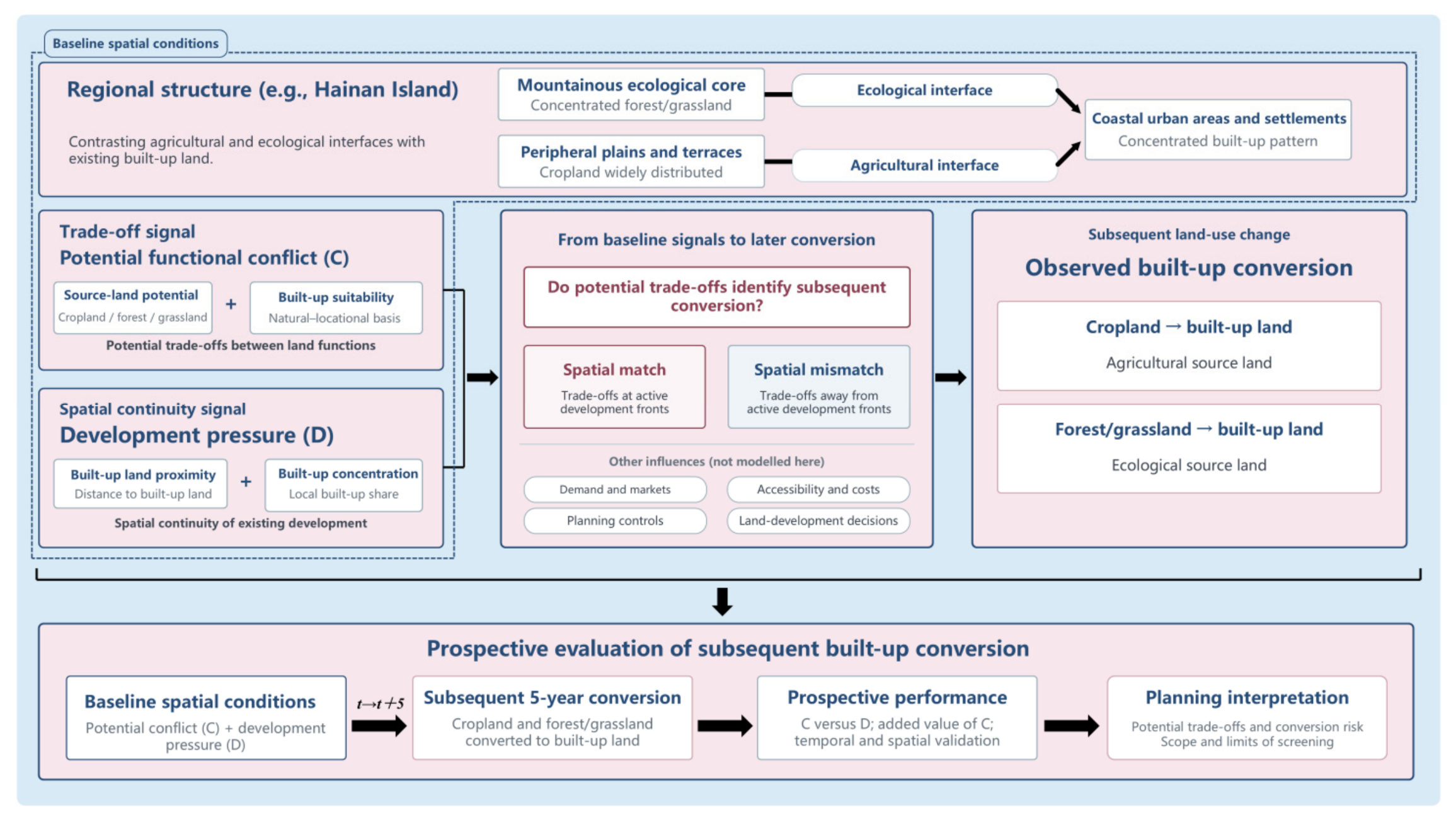
Potential functional conflict describes a baseline trade-off between alternative land allocations, whereas built-up conversion is a later land-use outcome. Their correspondence can depend on development demand, accessibility, planning controls, land supply, decisions on land development, tenure, and market conditions. High trade-off potential can persist without near-term conversion, while land with modest measured trade-offs can convert along active development frontiers.

Regional land-use patterns shape the interfaces between source lands and development fronts. We measured source-built-up contact, source-pixel distance to existing built-up land, and source patch structure to compare these interfaces between cropland and forest/grassland and between event and non-event cells. We then tested whether allowing the development-pressure relationship to differ by source type, or adding interface metrics, improved out-of-sample discrimination. These comparisons characterize the interfaces and assess their predictive relevance.

C is high where source-land functional potential and suitability for built development are both high and similar in magnitude. D instead describes continuity from the existing built-up pattern. Considering C and D together distinguishes four planning situations: trade-off potential at an active development frontier, trade-off potential away from the current frontier, development pressure with modest measured trade-offs, and locations where both signals are low. These situations distinguish trade-off intensity from transition imminence, two related but distinct spatial properties.

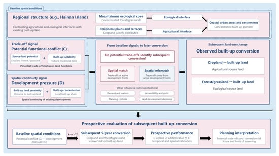
We tested whether baseline C identifies conversion during the following 5-year window by examining event coverage relative to the share of eligible observations in high-C locations, event rates along the C gradient, and the improvement in out-of-sample ranking when C is added to models containing development pressure and broad spatial structure. Temporal validation evaluates persistence into a later period, while geographically buffered validation tests transfer to spatially separated locations. Analyses by source type compare these relationships at urban-agricultural and urban-ecological interfaces. Figure 1 presents the conceptual framework and sequence of analyses.

Figure 1. Conceptual framework linking baseline spatial conditions to subsequent built-up land conversion.

2.2. Study Area

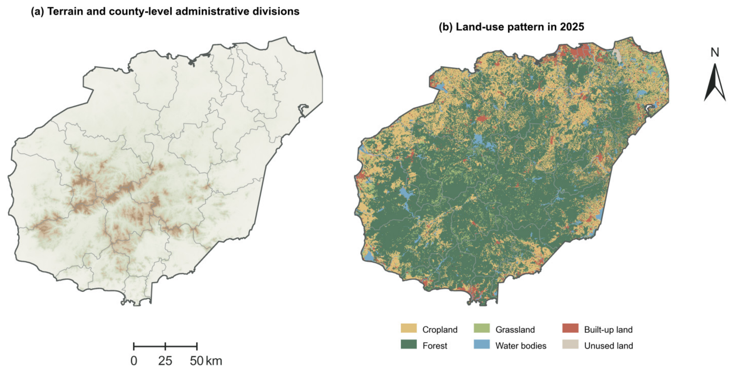
Hainan’s terrain rises from coastal plains through terraces and hills to the central mountains. Forest/grassland occupies much of the central and southern uplands, and cropland is concentrated on peripheral plains and terraces. Built-up land occurs mainly in cities, county seats, and coastal areas. Cropland forms a relatively continuous boundary with built-up land, whereas forest/grassland meets development chiefly at upland transitions and selected coastal sections. These distributions provide contrasting settings for examining conversion at the two interfaces.

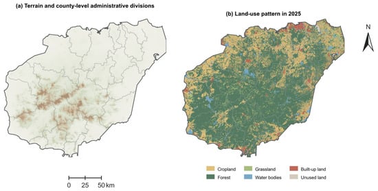
The study covers the terrestrial area of Hainan’s main island. We harmonized six land-use datasets and the environmental covariates on a 1 km grid, but identified conversion events from the original 30 m data. Figure 2 presents terrain, county-level administrative units, and the 2025 land-use distribution.

Figure 2. Terrain, county-level administrative divisions, and land-use patterns of Hainan Island in 2025. Map lines delineate the study area and do not necessarily depict accepted national boundaries.

2.3. Data Sources and Preprocessing

We used six 30 m land-use layers for 2000, 2005, 2010, 2015, 2020, and 2025 from the China Multi-Period Land Use/Land Cover Remote Sensing Monitoring Dataset (CNLUCC), provided by the Data Center for Resources and Environmental Sciences, Chinese Academy of Sciences (RESDC) [41]. Built-up land, used here as the umbrella term for construction land in the Chinese land-use context, includes the CNLUCC subclasses urban land, rural settlements, and other built-up land. These subclasses were combined to identify conversion from a non-built source to any built-up state, while their contributions to observed conversion were also reported separately. Cropland, forest, and grassland were retained as source classes. Forest and grassland transitions were identified separately at 30 m resolution and pooled for the main forest/grassland analysis; source-specific results were examined in sensitivity analyses.

Auxiliary data were used to measure functional potential and suitability for built development. Terrain was derived from the Copernicus GLO-30 digital elevation model (DEM), climate from WorldClim v2.1, and baseline vegetation from annual MOD13Q1 NDVI composites. SoilGrids, HydroRIVERS, and HydroLAKES provided soil and hydrographic variables [42,43,44,45,46,47]. Table 1 summarizes the datasets and their uses.

Table 1. Data sources and primary uses.

Data Category	Dataset or Product	Year(s)	Native Resolution	Source	Primary Use
Land use	CNLUCC	2000, 2005, 2010, 2015, 2020, 2025	30 m	Data Center for Resources and Environmental Sciences, Chinese Academy of Sciences (RESDC) [41]	Harmonization of land-use classes; identification of risk sets and conversion events
Elevation	Copernicus DEM GLO-30	Static	approx. 30 m	ESA [43]	Elevation, slope, and terrain relief
Climate	WorldClim v2.1 BIO1/BIO12	1970–2000 climatology	30 arc-seconds (≈1 km)	WorldClim [44]	Temperature and precipitation conditions
Vegetation	MOD13Q1 V061	Baseline year of each window (annual composite)	250 m	NASA LP DAAC [42]	Baseline vegetation conditions
Soil	SoilGrids 2.0	Static	250 m	ISRIC [47]	Properties of the 0–30 cm soil layer
Hydrography	HydroRIVERS/ HydroLAKES	Static	Vector	HydroSHEDS [45,46]	River network, water bodies, and distance metrics
Boundaries	Main-island and county-level administrative boundaries	Static	Vector	geoBoundaries (main-island boundary) and local administrative boundary data [48]	Study-area clipping and cartographic display

Vector-based metric calculations and the 1 km analysis grid used CGCS2000 (China Geodetic Coordinate System 2000), with the 3-degree Gauss–Krüger projection centered on 111° E (EPSG:4508). Raster calculations retained their native resolutions and projected grids, including those used to identify 30 m land-use transitions and derive terrain variables from the DEM. The resulting variables were then aggregated to the 1 km analysis grid.

Climate data were bilinearly resampled to a 100 m grid and averaged within each 1 km cell. Gaps within the land domain were filled by linear interpolation, with nearest-neighbor interpolation used where gaps remained. Soil organic carbon and pH values were multiplied by 0.1 before depth weighting over 0–5, 5–15, and 15–30 cm. Annual NDVI used quality-screened observations (SummaryQA ≤ 1) from the entire baseline year.

Hydrographic features were selected within a 2 km buffer around the combined area of the analysis cells; density and area proportions used the complete grid area. Distance to a lake was set to zero only where the grid centroid intersected the lake polygon. Empty hydrographic intersections were assigned zero length or area, whereas unavailable regional features were recorded as missing values.

2.4. Measurement of Core Variables

For P_s and Pᵤ, indicators were transformed according to their suitability direction before standardization. Temperature T and soil pH used t = −|T − 24| and t = −|pH − 6.5|, respectively; otherwise, t = x. Transformed values were standardized as z = clip[(t − q₂)/(q₉₈ − q₂), 0, 1], where q₂ and q₉₈ are the source-specific 2nd and 98th percentiles estimated from the original 2000–2015 training domain. If q₉₈ ≤ q₂, the upper bound was set to q₂ + 1. Positive and reference-centered indicators used z, whereas inverse indicators used 1 − z. Distance indicators did not use logarithmic or exponential decay. The fitted transformations were applied unchanged to later validation and test observations; Pᵤ scaling was estimated separately for the two source types.

Temperature and soil pH were treated as reference-centered cropland indicators using 24 °C and pH 6.5 as generalized reference values rather than universal crop-specific physiological optima. These values fall within favorable thermal and near-neutral soil-reaction ranges reported for many warm-region crops in established land-evaluation guidance [49]. For the Hainan reference model, lower elevation, slope, and relief were treated as more favorable for cropland and built development, consistent with land-suitability frameworks in which gentler, lower-relief terrain imposes fewer cultivation and construction constraints [49,50]. In contrast, higher terrain values were assigned positive directions for forest/grassland P_s to reflect the observed concentration of these source functions in Hainan’s central and southern uplands [35,36,37,38], rather than a universal ecological preference.

The reference P_s and Pᵤ indices were arithmetic means of the available standardized components. Equal weighting provided a common reference without assigning greater a priori importance to individual indicators. Nominal complete-data weights were 1/11 for cropland P_s, 1/9 for forest/grassland P_s, and 1/6 for Pᵤ. Missing components were omitted, and the remaining weights renormalized rather than assigning missing values zero. Entropy- and CRITIC-weighted alternatives used the same component sets, with weights estimated from complete training observations and renormalized over the available components when applied.

2.4.1. Source-Land Functional Potential

P_s represents the relative natural support for maintaining the source-land function, following multifunctional land-assessment and conflict-identification studies [12,13,14,15,16,17,18,19,20]. Cropland P_s used 11 indicators covering elevation, slope, terrain relief, temperature, precipitation, soil organic carbon, soil pH, river proximity and density, and lake proximity and area. Forest/grassland P_s used nine indicators covering elevation, slope, terrain relief, precipitation, annual NDVI, and the same four hydrographic measures. Table 2 reports the complete set of indicators used, data source, calculation rule, and suitability direction.

Table 2. Indicator definitions and construction rules for source-land functional potential, built-up suitability, potential functional conflict, and development pressure.

Indicator	Data Source	Calculation/Preprocessing	Direction
A. Cropland Ps—11 indicators
Mean elevation	Copernicus DEM GLO-30	Mean valid 30 m elevation within the cell.	−
Mean slope	Copernicus DEM GLO-30	Slope from the 30 m DEM gradient; mean slope (degrees) within each cell.	−
Elevation range within the analysis cell	Copernicus DEM GLO-30	Maximum minus minimum valid elevation within the cell.	−
Annual mean temperature	WorldClim v2.1 (BIO1/BIO12)	WorldClim BIO1; aggregated to the 1 km cell; t = −|T − 24| before scaling.	Reference center: 24 °C
Annual precipitation	WorldClim v2.1 (BIO1/BIO12)	WorldClim BIO12; aggregated to the 1 km cell.	+
Soil pH (0–30 cm)	ISRIC SoilGrids 2.0	Depth-weighted mean of 0–5, 5–15 and 15–30 cm layers; t = −|pH − 6.5|.	Reference center: pH 6.5
Soil organic carbon (0–30 cm)	ISRIC SoilGrids 2.0	Depth-weighted 0–30 cm mean (g kg−1) from the three SoilGrids depth layers.	+
Distance to nearest river	HydroRIVERS v1.0	Minimum Euclidean distance from the grid centroid to HydroRIVERS.	−
River length density	HydroRIVERS v1.0	River length intersecting the cell (km) divided by cell area (km2).	+
Distance to nearest lake	HydroLAKES v1.0	Minimum Euclidean distance from the grid centroid to HydroLAKES; zero where the centroid intersects a lake.	−
Lake area proportion	HydroLAKES v1.0	Lake area intersecting the cell divided by total cell area.	+
B. Forest/grassland Ps—9 indicators
Mean elevation	Copernicus DEM GLO-30	Mean valid 30 m elevation within the cell.	+
Mean slope	Copernicus DEM GLO-30	Slope from the 30 m DEM gradient; mean slope (degrees) within each cell.	+
Elevation range within the analysis cell	Copernicus DEM GLO-30	Maximum minus minimum valid elevation within the cell.	+
Annual precipitation	WorldClim v2.1 (BIO1/BIO12)	WorldClim BIO12; aggregated to the 1 km cell.	+
Annual median NDVI	MOD13Q1 V061	Median of quality-screened MOD13Q1 observations for the baseline year; aggregated to 1 km.	+
Distance to nearest river	HydroRIVERS v1.0	Minimum Euclidean distance from the grid centroid to HydroRIVERS.	−
River length density	HydroRIVERS v1.0	River length intersecting the cell (km) divided by cell area (km2).	+
Distance to nearest lake	HydroLAKES v1.0	Minimum Euclidean distance from the grid centroid to HydroLAKES; zero where the centroid intersects a lake.	−
Lake area proportion	HydroLAKES v1.0	Lake area intersecting the cell divided by total cell area.	+
C. Built-up suitability Pᵤ—6 indicators
Mean elevation	Copernicus DEM GLO-30	Mean valid 30 m elevation within the cell.	−
Mean slope	Copernicus DEM GLO-30	Slope from the 30 m DEM gradient; mean slope (degrees) within each cell.	−
Elevation range within the analysis cell	Copernicus DEM GLO-30	Maximum minus minimum valid elevation within the cell.	−
Mean distance to fixed coastline	Fixed Hainan main-island mask	Mean 30 m Euclidean distance from land pixels to the fixed main-island coastline within each cell.	−
Distance to nearest river	HydroRIVERS v1.0	Minimum Euclidean distance from the grid centroid to HydroRIVERS.	−
Distance to nearest lake	HydroLAKES v1.0	Minimum Euclidean distance from the grid centroid to HydroLAKES; zero where the centroid intersects a lake.	−
D. Derived indices
Potential functional conflict	Derived from Ps and Pᵤ	C = [(Ps + Pᵤ)/2] × [1 − |Ps − Pᵤ|].	Higher = suitability overlap/potential trade-off
Development pressure	Baseline CNLUCC built-up pattern	Equal-weight mean of standardized proximity to existing built-up land and local built-up share in the 33 × 33-pixel reference window.	Higher = development continuity

Note: “+” and “−” indicate increasing and decreasing suitability with the raw indicator value, respectively. Reference-centered transformations apply to temperature and soil pH. Data sources and preprocessing are described in Section 2.3; indicator transformations, normalization, weighting, and missing-data treatment are specified in Section 2.4.

2.4.2. Suitability for Built Development

Suitability for built development (Pᵤ) was calculated from six indicators: mean elevation, mean slope, terrain relief, mean distance to the fixed coastline, distance to the nearest river, and distance to the nearest lake. Terrain and distance indicators were oriented so that less restrictive terrain and greater locational accessibility received higher standardized suitability scores. Proximity to existing built-up land was excluded from Pᵤ so that the suitability-overlap index remained distinct from development continuity (Table 2).

2.4.3. Suitability-Overlap-Based Potential Land-Use Functional Conflict

We measured potential functional conflict from the joint strength and balance of two competing potentials for the same land unit: retaining its source-land function (P_s) and converting it to built-up land (Pᵤ). Because these states cannot be fully realized simultaneously at one location, high values of both potentials indicate a potential allocation trade-off. This definition distinguishes competition between alternative allocations from multifunctional suitability alone. Following suitability-based and multifunctional conflict-assessment approaches that identify potential competition through functional overlap [12,13,14,15,16,17,18,19,20], we calculated:

C = [(P_s + Pᵤ)/2] × [1 − |P_s − Pᵤ|]

(1)

The first term, M = (P_s + Pᵤ)/2, measures the joint magnitude of support for the two alternatives. The second, B = 1 − |P_s − Pᵤ|, reduces the score where one alternative dominates. Their product is high where both alternatives are strongly supported and similar in magnitude. The reference formulation treated the two allocation alternatives symmetrically, with equal weights and a linear balance term. Sensitivity analyses varied their relative weights from 0.30/0.70 to 0.70/0.30 and the balance exponent across γ = 0.5, 1, and 2. We also reconstructed the suitability indices using entropy and CRITIC weights and compared three overlap formulations: minimum, product, and harmonic mean.

2.4.4. Development Pressure

Built-up land often expands through edge growth, infill, and development adjoining existing settlements [33,34,51]. D combines mean distance to baseline built-up land with the local share of baseline built-up land. The built-up share was first calculated on the 30 m land-use raster using a 33 × 33-pixel moving window (approximately 0.99 × 0.99 km) and was then aggregated to the 1 km analysis grid. Thus, the reference window defines the local raster support of the calculation rather than a single neighborhood centered on each 1 km cell, and it was not optimized as an influence radius. The built-up share used the fixed main-island mask employed in the original preprocessing as its denominator; land-use NoData pixels within that mask therefore contributed to the denominator as non-built pixels. Both components were oriented so that higher values indicated stronger development continuity and were equally weighted. Sensitivity analyses repeated the built-up-share calculation with 17 × 17 (approximately 0.5 km) and 67 × 67 (approximately 2 km) windows and separately examined the denominator using only classified pixels. Keeping D separate from Pᵤ prevents proximity to existing development from entering C (Table 2).

2.5. Built-Up Land Conversion Events and Risk Sets

A cell was included in a source-specific risk set when the source-land type occupied at least 10% of the cell at the start of each window. Risk sets were regenerated for each window, and partially converted cells remained eligible, provided that they met the threshold.

To reduce noise, conversion patches had to contain at least 25 contiguous 30 m pixels under an eight-neighbor connectivity rule, approximately 2.25 ha. A 1 km cell was classified as an event when the converted area reached both 0.01 km² and 1% of its initial source area. Reference thresholds were chosen to maintain adequate event counts and source-land samples across the five observation windows. Sensitivity analyses varied the initial source share from 5% to 15%, minimum patch size from 16 to 36 pixels, absolute converted area from 0.005 to 0.02 km², and relative converted share from 0.5% to 2%. Looser and stricter combinations were also tested. We compared event counts, direct rankings by C and D, and the paired M2–M3 results across these definitions.

2.6. Spatial Correspondence and Expansion-Configuration Analysis

To compare the indicators across periods and source-land types, continuous scores were converted into mean rank percentiles within each period- and source-specific risk set.

p_i = [(r_i − 0.5)/N] × 100

(2)

where p_i is the mean-rank percentile, r_i is the mean rank, with ties assigned their average rank, and N is the risk-set size. Subtracting 0.5 places each rank at the midpoint of its empirical percentile interval. We measured event coverage within the highest 10%, 20%, and 30% of C and D. Continuous ranking performance was evaluated using the area under the precision-recall curve (PR-AUC), which is appropriate for rare conversion events [52,53]. Event rates were also compared across deciles to determine whether conversion increased systematically along either indicator, beyond the choice of a high-value threshold.

We cross-classified the quintiles of C and D. Event lift was defined as the ratio of the C–D category-specific event rate to the overall period-specific event rate. We also used the 80th percentile to define four configurations: high-C/high-D, high-C/low-D, low-C/high-D, and low-C/low-D.

2.7. Model Estimation, Validation, and Risk Mapping

We fitted generalized additive models (GAMs) with a binomial complementary log–log link for the rare binary conversion events [54], allowing nonlinear covariate and spatial effects [55]. Models were estimated using R 4.6.0 (R Foundation for Statistical Computing, Vienna, Austria) with mgcv 1.9-4 via mgcv::bam, using fast restricted maximum likelihood (fREML), discrete fitting, and shrinkage selection. Other data processing and visualization were performed using Python 3.11.9 (Python Software Foundation, Beaverton, OR, USA). We compared six candidate models to separate the contributions of broad temporal–spatial structure, potential functional conflict, and development continuity (Table 3). Thin-plate regression splines used k = 6 for one-dimensional covariate smooths and k = 200 for the two-dimensional spatial smooth; sensitivity to alternative spatial-basis dimensions is reported in Section 3.5. The M5 interaction used k = (5, 5). P_s, Pᵤ, and C were not entered together because C is a deterministic function of the two potentials. All models were evaluated under temporal and buffered spatial validation. The paired M2–M3 comparison estimates the information added by C after accounting for development pressure and broad spatial structure.

Table 3. Candidate generalized additive models and their inferential roles.

Model	Linear Predictor Terms	Inferential Role
M0	period + s(x, y, k = 200)	Broad temporal and spatial structure
M1	period + s(C, k = 6) + s(x, y, k = 200)	Increment from potential functional conflict (C)
M2	period + s(D, k = 6) + s(x, y, k = 200)	Development-pressure benchmark plus spatial structure
M3	period + s(C, k = 6) + s(D, k = 6) + s(x, y, k = 200)	Incremental value of C beyond D
M4	period + s(Ps, k = 6) + s(Pᵤ, k = 6) + s(D, k = 6) + s(x, y, k = 200)	Uncombined source and built-development potentials
M5	period + s(C, k = 6) + s(D, k = 6) + ti(C, D, k = (5, 5)) + s(x, y, k = 200)	C–D interaction

Note: C = potential functional conflict; D = development pressure; P_s = source-land functional potential; Pᵤ = suitability for built development.

Models were trained on the 2000–2015 data and validated temporally against 2015–2020 observations. Spatial transfer within the 2000–2015 data was evaluated with five outer validation folds constructed from 10 km spatial blocks and a 10 km exclusion buffer around each held-out fold, with all observations from the same grid location assigned to the same fold [56,57]. Residual spatial dependence was estimated separately from the training observations in each fold; the effective range was 7.5 km for both source types, so the 10 km exclusion distance was retained. This design follows the broader principle that geospatial model assessment should separate training and evaluation locations when the intended prediction task involves spatial transfer [58]. Temporal validation assesses persistence into a later period within the same regional system, whereas buffered spatial validation assesses transfer to geographically more independent locations.

For near-term risk mapping, M2 was retained after the final validation comparison. M3 would replace M2 only if the paired increase in PR-AUC had a 95% confidence interval above zero under both temporal and buffered spatial validation; this criterion was not met for either source type. M2 incorporated development pressure and spatial structure:

g[Pr(Y_it = 1)] = α_t + f(D_it) + s(x_i, y_i)

(3)

where g is the complementary log–log link, α_t is the period effect, f(D_it) is the smooth function of development pressure, and s(x_i, y_i) is the spatial smooth. For temporal validation, the 2015–2020 observations were assigned the latest period level in the 2000–2015 training data (2010–2015). Following the temporal and buffered spatial validation, M2 and M3 were refitted to the 2000–2020 data and evaluated on the 2020–2025 window; these observations were similarly assigned the latest fitted period level (2015–2020). Assigning a single period level to each evaluation window produced a common shift in the linear predictor and did not affect the within-window rankings used for evaluation. The event and risk-set thresholds had been informed by all five observation windows, so we treated the 2020–2025 analysis as an out-of-time evaluation rather than a fully independent test set. M2 produced the risk maps, and its comparison with M3 tested whether C added information in the later period. We estimated uncertainty in PR-AUC and event coverage from 1000 resamples of unique 10 km spatial blocks, taking the 2.5th and 97.5th percentiles as the 95% confidence limits.

2.8. Sensitivity Analyses

Sensitivity analyses examined the main choices underlying C, event identification, source aggregation, spatial support, D, and model specification. For C, we varied relative P_s/Pᵤ weights, balance penalties, overlap functions, and entropy- and CRITIC-weighted component indices. Event analyses varied source-share, patch-size, absolute-area, and relative-area thresholds. Forest and grassland were analyzed separately, and aligned 500 m and 2 km grids were compared with the 1 km reference grid to assess sensitivity to the modifiable areal unit problem (MAUP) [59]. The main cross-scale event rule used a converted-area threshold equal to 1% of the analysis-cell area, with a secondary fixed 0.01 km² rule.

Further analyses varied the spatial smooth, checked the 10 km exclusion distance against fold-specific residual ranges, compared D with proximity-only and built-up-share-only benchmarks, and varied the built-up-share neighborhood in D from approximately 0.5 to 2 km. For the neighborhood-scale sensitivity, scaling parameters for the alternative built-up-share component were re-estimated from the training data of each validation split and then held fixed for its validation data; C and the distance component retained their reference preprocessing. All three neighborhood sizes, including the 1 km case, were refitted using the same sensitivity-analysis procedure to ensure comparability. A separate calculation also recomputed the neighborhood share after excluding land-use NoData pixels from the denominator.

Three interface metrics were derived from the 30 m baseline land-use data within each 1 km cell. Source-built-up contact-edge density was calculated from shared four-neighbor boundaries, in kilometers of contact per square kilometer of valid land. We also calculated the mean distance of source pixels to existing built-up land and source patch density, defined as eight-neighbor connected source patches per square kilometer of source land. Frontier exposure was summarized descriptively but excluded from models containing contact-edge density because the two were nearly collinear.

Distributional summaries and rank-biserial effect sizes were used to compare event and non-event cells. We then compared a pooled model with a common smooth of D across source types against a model with separate D smooths for the two source types. A third model added contact-edge density and patch-density smooths for each source type. All three were evaluated using the temporal and buffered spatial validation designs applied in the main analysis.

3. Results

3.1. Temporal Change and Spatial Progression of Built-Up Land Conversion

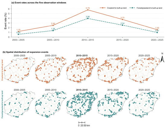
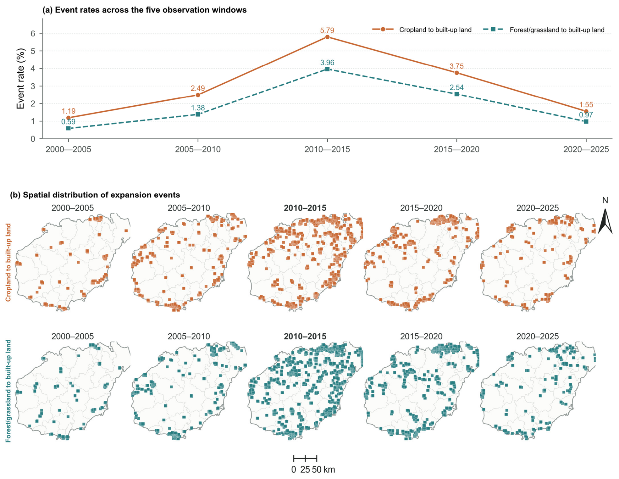
Conversion-event rates for both source types peaked in 2010–2015 and declined thereafter (Table 4; Figure 3a). The cropland rate rose from 1.188% to 5.790% before falling to 1.554% in 2020–2025. The forest/grassland rate increased from 0.585% to 3.961%, then declined to 0.973%. Cropland had a higher event rate in every window.

Table 4. Risk sets, event counts, and event rates for the two built-up land expansion types.

Period	Cropland Risk-Set Cells	Cropland Events	Cropland Event Rate (%)	Forest/Grassland Risk-Set Cells	Forest/Grassland Events	Forest/Grassland Event Rate (%)
2000–2005	17,766	211	1.188	30,766	180	0.585
2005–2010	17,419	433	2.486	30,660	422	1.376
2010–2015	17,616	1020	5.790	30,675	1215	3.961
2015–2020	17,412	653	3.750	30,558	775	2.536
2020–2025	17,444	271	1.554	30,527	297	0.973

Figure 3. Temporal changes and spatial distribution of the two built-up land conversion types. (a) Event rates across five windows. (b) The upper and lower rows show the cropland and forest/grassland event cells, respectively. Map lines delineate the study area and do not necessarily depict accepted national boundaries.

The destination subclasses differed among source lands. Across the five intervals, 24.63% of the cropland conversion area became urban land, 23.06% became rural settlements, and 52.32% became other built-up land. The corresponding shares were 13.41%, 15.14%, and 71.45% for forest and 15.77%, 17.61%, and 66.62% for grassland. The pooled outcome combines transitions to built-up land that differ in their destination composition.

Conversion events were initially scattered around settlements and peripheral areas. They later became concentrated in the northern urban cluster and along the eastern and southern coasts (Figure 3b). Both source types formed broader conversion belts during the 2010–2015 peak, followed by contraction toward fewer settlement margins after 2015. Cropland conversion was more common on plains and terraces and along urban edges. Forest/grassland conversion was more common in hill transition zones and along mountain margins and coastal ecological edges.

3.2. Prospective Performance of Potential Functional Conflict and Development Pressure

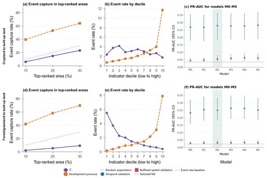
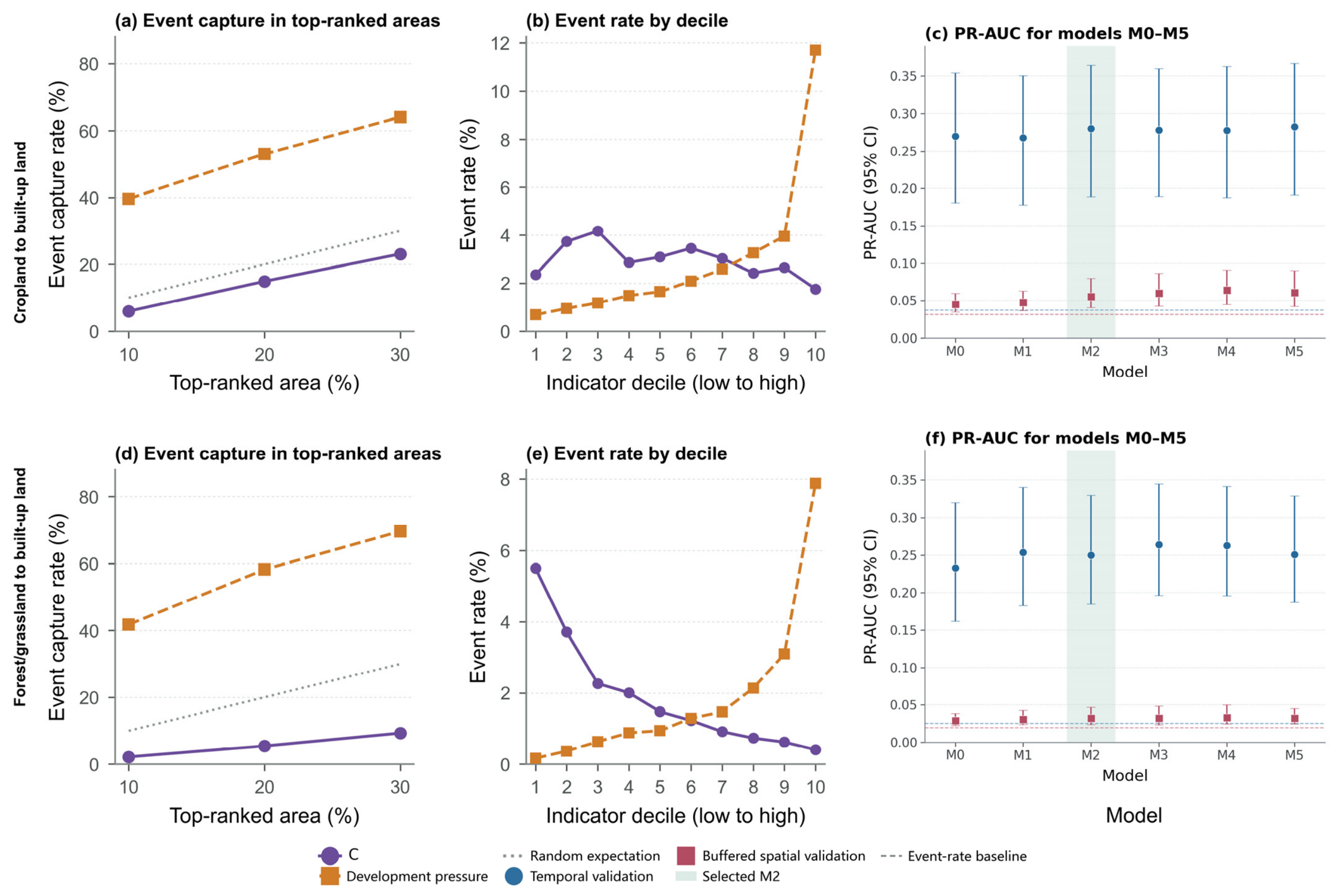
High-C areas contain less than their proportional share of subsequent conversion. Across the five windows, the highest 20% of C captured 14.91% of cropland events and 5.43% of forest/grassland events, both below the 20% share of eligible grid-period observations represented by this group. By comparison, the highest 20% of D captured 53.05% and 58.22% of the two event types, respectively (Figure 4a,d). The continuous rankings showed the same contrast: D achieved higher PR-AUC and a steeper positive event-rate gradient, whereas C did not show a monotonic positive event gradient and forest/grassland conversion declined at the highest C ranks (Figure 4b,e). The configuration analysis in Section 3.3 places this low capture in context: high-C locations span different levels of development pressure, and their conversion rates do not follow a uniformly inverse relationship with C.

Figure 4. Prospective identification of built-up land conversion using potential functional conflict (C), development pressure, and their corresponding model combinations. Note: Panels (a–c) show results for cropland, and panels (d–f) show results for forest/grassland. The left and middle panels present pooled results from the five risk sets, whereas the right panels show the results of the 2015–2020 temporal validation and buffered spatial validation within the 2000–2015 data. M0–M5 denote the six model specifications defined in Table 3, and pale green indicates M2, which contains development pressure and broad spatial structure.

The relative performance of M0–M5 varied with source type and validation design (Table 5). In temporal validation for cropland, PR-AUC ranged from 0.2679 (M1) to 0.2827 (M5); M2, M3, M4, and M5 had similar point estimates. For forest/grassland, M3 had the highest temporal estimate (0.2640), closely followed by M4 (0.2628). Buffered spatial validation reduced performance for every model. M4 had the highest spatial estimate for cropland (0.0640) and forest/grassland (0.0335), although differences among the models with higher point estimates were small relative to their uncertainty.

Table 5. Out-of-sample performance of the six candidate models under temporal and buffered spatial validation.

Panel A. PR-AUC (95% CI).
Model	Cropland Temporal	Cropland Buffered Spatial	Forest/Grassland Temporal	Forest/Grassland Buffered Spatial
M0	0.2698 (0.1810, 0.3543)	0.0454 (0.0348, 0.0598)	0.2330 (0.1620, 0.3202)	0.0290 (0.0225, 0.0388)
M1	0.2679 (0.1779, 0.3506)	0.0477 (0.0367, 0.0630)	0.2537 (0.1830, 0.3403)	0.0309 (0.0236, 0.0429)
M2	0.2803 (0.1891, 0.3645)	0.0556 (0.0405, 0.0797)	0.2501 (0.1850, 0.3299)	0.0325 (0.0239, 0.0469)
M3	0.2782 (0.1894, 0.3602)	0.0599 (0.0426, 0.0865)	0.2640 (0.1966, 0.3450)	0.0323 (0.0233, 0.0486)
M4	0.2777 (0.1876, 0.3630)	0.0640 (0.0450, 0.0907)	0.2628 (0.1959, 0.3413)	0.0335 (0.0245, 0.0500)
M5	0.2827 (0.1917, 0.3672)	0.0608 (0.0424, 0.0902)	0.2505 (0.1873, 0.3290)	0.0326 (0.0246, 0.0453)
Panel B. Event Coverage Within the Highest 20% Predicted-Risk Cells (95% CI).
Model	Cropland Temporal	Cropland Buffered Spatial	Forest/Grassland Temporal	Forest/Grassland Buffered Spatial
M0	67.99% (56.11–77.58%)	36.30% (26.40–46.60%)	75.87% (67.49–82.73%)	30.93% (22.60–39.33%)
M1	67.23% (56.40–76.82%)	36.78% (27.05–47.48%)	77.29% (69.70–83.42%)	32.58% (24.38–40.99%)
M2	73.20% (62.44–81.47%)	41.41% (31.31–51.98%)	77.81% (70.45–83.90%)	31.43% (23.27–39.68%)
M3	72.43% (62.01–80.57%)	42.49% (32.48–53.04%)	78.06% (70.84–83.87%)	31.70% (23.32–40.17%)
M4	73.66% (63.86–81.25%)	44.05% (34.98–54.25%)	78.97% (71.87–84.68%)	33.68% (25.04–42.20%)
M5	71.98% (61.36–80.45%)	41.83% (32.11–52.08%)	78.58% (71.47–84.26%)	34.29% (25.82–42.55%)

Note: PR-AUC is average precision. All models within a source type and validation design were evaluated on the same held-out observations. Temporal validation used 2015–2020 observations, whereas buffered spatial validation used the 2000–2015 observations in five geographically separated outer folds with a 10 km exclusion buffer. Confidence intervals were obtained from 1000 spatial-block bootstrap resamples. The 2020–2025 M2–M3 comparison is reported in Section 3.4.

Adding C to the development-pressure model did not improve discrimination consistently across both validation designs for either source type. With the main spatial smooth, k = 200, the paired M3−M2 difference was −0.0021 in temporal validation and +0.0042 in buffered spatial validation for cropland. For forest/grassland, it was +0.0140 temporally and approximately zero (−0.0003) spatially.

3.3. C–D Configurations and Event Concentration

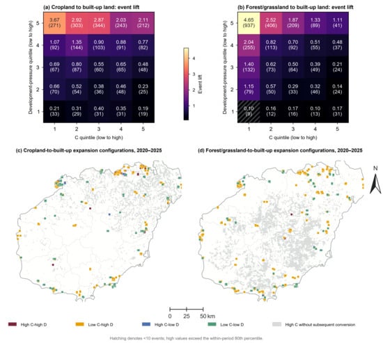
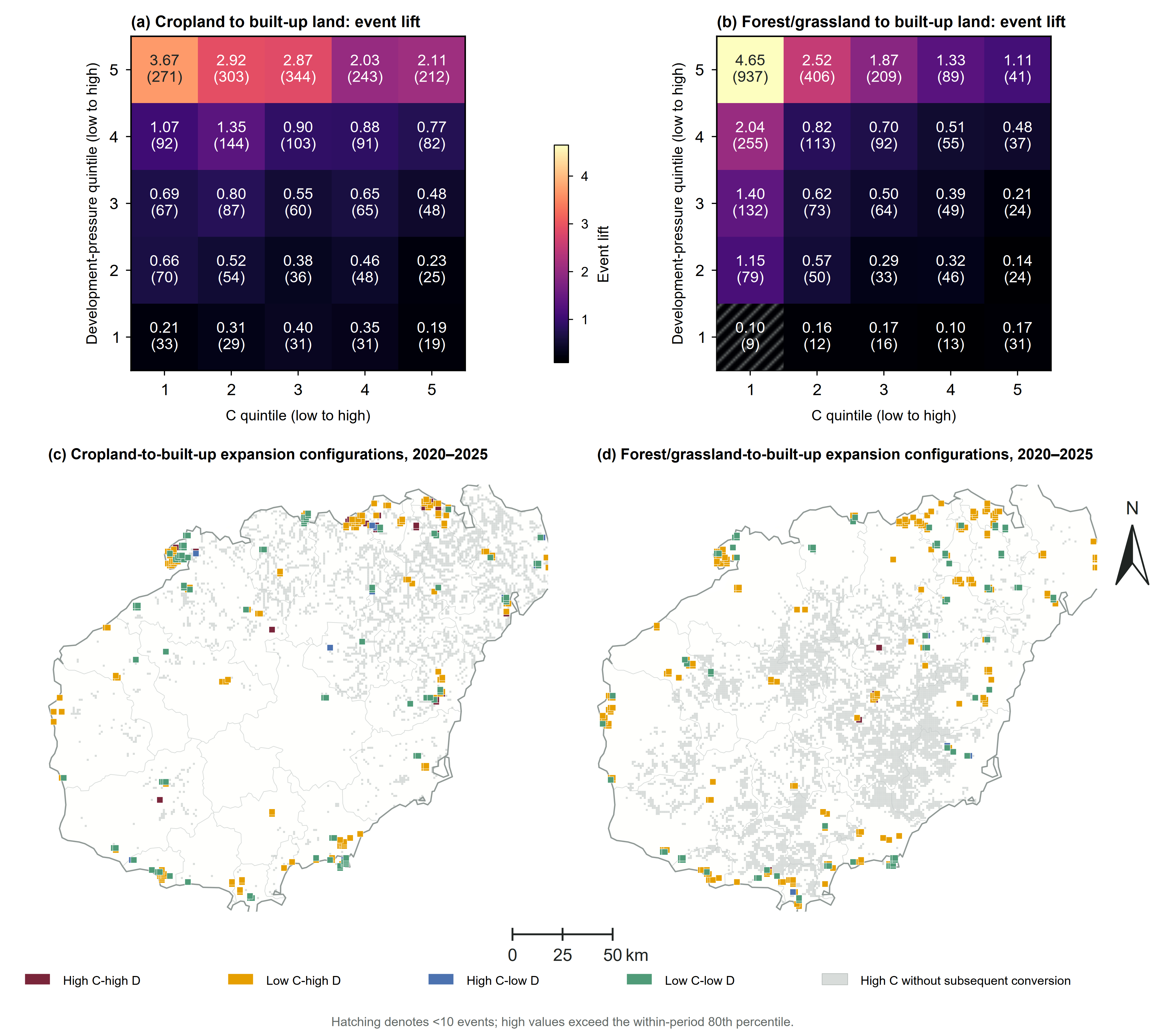
Event concentration increased with D, with no comparable increase along C (Figure 5a,b). Lift generally exceeded 1 in the highest D quintile. Within that quintile, cropland lift ranged from 2.03 to 3.67 across the C quintiles, whereas forest/grassland lift declined from 4.65 to 1.11. Conversion was thus concentrated near existing development even where C was low.

Figure 5. Event concentration and expansion configurations under different combinations of potential functional conflict (C) and development pressure (D). Note: Potential functional conflict (C) and development pressure (D) are classified into within-period quintiles. Heat maps show pooled event lifts, event counts, and hatched cells indicating areas with fewer than 10 events. The 80th percentile was used to distinguish high and low values. The maps show the 2020–2025 configurations; gray marks indicate high-C cells without conversion. Map lines delineate the study area and do not necessarily depict accepted national boundaries.

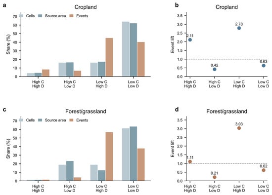
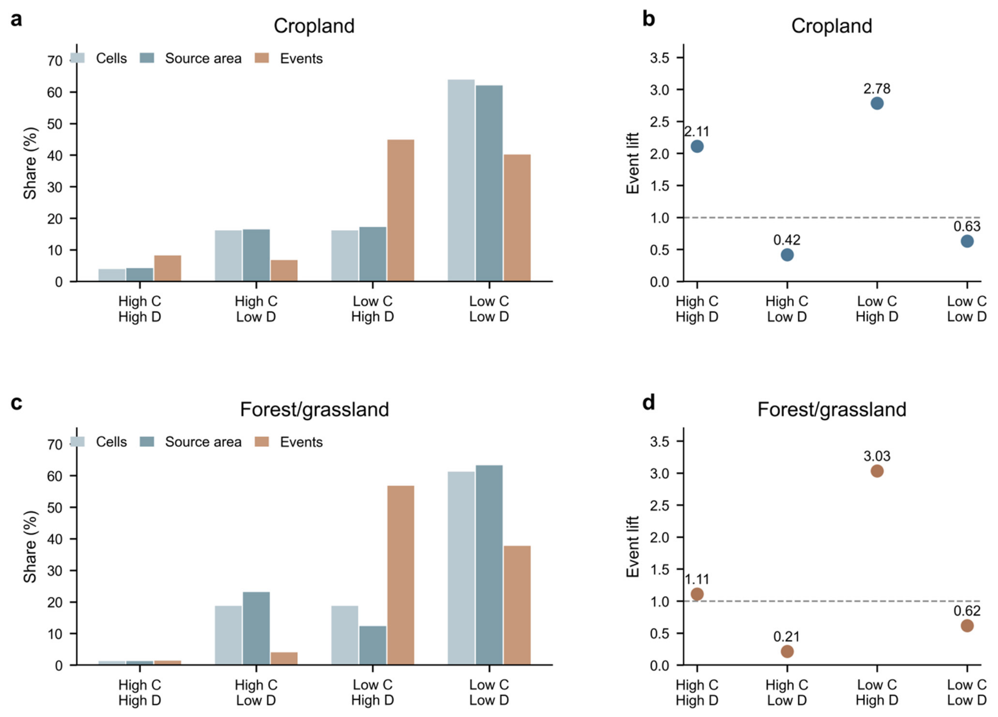
Across the five windows, low-C/high-D locations contained 44.86% of cropland events and 56.80% of forest/grassland events, despite occupying a smaller share of the observations and source-land area than low-C/low-D locations. For cropland, this configuration occupied 16.12% of grid-period observations and 17.22% of source-land area exposure, with an event rate of 8.22% and a lift of 2.78. For forest/grassland, it occupied 18.72% of observations and 12.35% of source-land area exposure but contained 56.80% of events; its event rate was 5.72%, and lift was 3.03.

Low-C/low-D was the largest exposure category for both source types, yet had substantially lower event rates. High-C/high-D contained smaller event shares, 8.19% for cropland and 1.42% for forest/grassland, and had lower pooled event rates than low-C/high-D. The pattern varied across periods: low-C/high-D contained the largest event share in all five forest/grassland windows, while low-C/low-D contained slightly more cropland events in 2005–2010 and 2010–2015. Event concentration in low-C/high-D locations reflects both their extent and their elevated within-category event rates (Figure 6).

Figure 6. Exposure and event concentration across the four C × D configurations. (a) Cropland shares of cells, source-land area, and events; (b) cropland event lift; (c) forest/grassland shares of cells, source-land area, and events; (d) forest/grassland event lift. Note: Shares pool five grid-period observation windows; source-land area is therefore an exposure measure summed across periods rather than a non-repeated geographic area. Event lift is the configuration-specific event rate divided by the overall event rate for the corresponding source type. High and low C and D follow the within-period 80th-percentile classification used in Figure 5.

3.4. Near-Term Expansion Risk and Spatial Transferability

Temporal discrimination exceeded buffered spatial discrimination across all six models (Table 5). Relationships persisted more strongly into a later period within Hainan than across geographically separated locations. This difference extended across the model set, regardless of whether C was included.

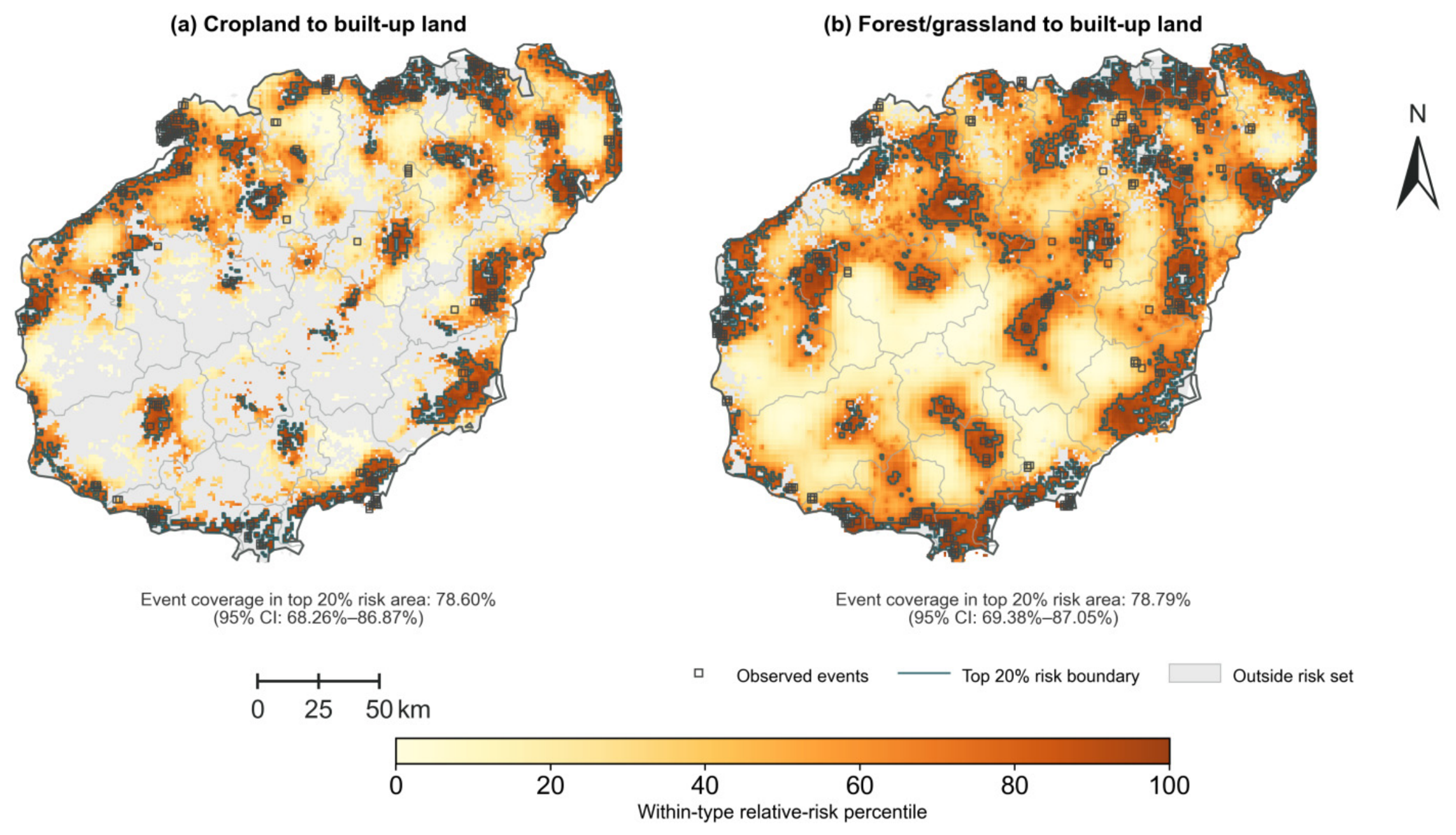
M2 and M3 performed similarly in the 2020–2025 out-of-time evaluation. Because event and risk-set thresholds had been informed by all five observation windows, this analysis was an out-of-time evaluation rather than a fully independent test set. Adding C increased cropland PR-AUC from 0.1382 to 0.1412, a paired difference of +0.0030 (95% CI −0.0069 to +0.0123). Coverage within the highest 20% of predicted risk increased by 1.48 percentage points (95% CI 0.00 to 3.38 percentage points). For forest/grassland, PR-AUC changed from 0.0942 to 0.0948, a difference of +0.0006 (95% CI −0.0088 to +0.0059), while the top-20% event coverage changed by −0.67 percentage points (95% CI −2.86 to +1.80 percentage points). These estimates provide no clear evidence that adding C improved discrimination in 2020–2025. The retained M2 mapping model captured 78.60% of cropland events and 78.79% of forest/grassland events within the highest-ranked 20% of eligible grid cells.

The M2 risk surfaces followed the existing built-up pattern, with different cluster shapes reflecting the distribution of each source land (Figure 7). Cropland risk formed continuous clusters around the northern urban cluster, the southeastern coast, and county seats. Forest/grassland risk extended along the island’s flanks and the margins of the central and southern mountains.

Figure 7. Relative expansion risk and observed conversions of cropland and forest/grassland to built-up land, 2020–2025. Note: Relative risk is estimated using M2, which includes development pressure and the broad spatial structure. Colors indicate within-type risk percentiles; these rankings should not be compared in absolute terms across land types. Boundaries delineate the highest-ranked 20% of eligible grid cells, and open symbols indicate the observed events. Map lines delineate the study area and do not necessarily depict accepted national boundaries.

3.5. Sensitivity of the Main Results

Changing the formulation of C altered local C rankings but had little effect on the main comparison at 1 km. When the relative contribution of P_s varied from 0.30 to 0.70, Spearman correlations with the original C were 0.985–0.996 for cropland and 0.957–0.989 for forest/grassland. Across weighting and overlap formulations, the top-20% event capture ranged from 10.66% to 22.72% for cropland and from 4.50% to 14.85% for forest/grassland. With the main spatial model, adding C under any alternative failed to improve performance consistently across both validation designs for either source type.

Forest/grassland results were more sensitive to the representation of broad spatial structure than cropland results. For cropland, the temporal M3−M2 difference remained negative when the spatial term was omitted and when k varied from 50 to 400; the buffered spatial difference was small and non-monotonic. For forest/grassland, the temporal difference declined from +0.0408 without the spatial term to +0.0135 at k = 400, while the spatial difference remained non-monotonic. Concurvity diagnostics indicated greater overlap between C and broad spatial structure for forest/grassland. The residual range remained 7.5 km, below the 10 km exclusion distance.

Alternative event definitions changed event counts but preserved the contrast between C and D at 1 km. Across the 11 threshold specifications, cropland M3−M2 ΔPR-AUC ranged from −0.0024 to +0.0015 temporally and from +0.0027 to +0.0047 spatially. Forest/grassland differences ranged from +0.0108 to +0.0152 temporally and from −0.0006 to +0.0016 spatially. Reducing minimum patch size from 25 to 16 pixels increased 2015–2020 event counts from 653 to 670 for cropland and from 775 to 795 for forest/grassland. D had higher direct PR-AUC and top-20% event coverage than C across threshold scenarios and all five periods.

Separate analyses of forest and grassland retained the direct ranking advantage of D over C but showed different event frequencies and uncertainty. Forest event rates were 0.57%, 1.32%, 3.82%, 2.44%, and 0.91% across the five windows; grassland rates were 0.39%, 0.98%, 2.20%, 1.42%, and 0.67%. Adding C to M2 increased temporal PR-AUC by +0.0133 for forest (95% CI +0.0040 to +0.0230) and +0.0067 for grassland (95% CI −0.0582 to +0.0303). Buffered spatial increments were +0.0002 (95% CI −0.0014 to +0.0017) and +0.0070 (95% CI −0.0030 to +0.0263), respectively. The wider intervals for grassland reflect its smaller event sample, which is obscured in the pooled forest/grassland comparison.

C and D retained similar spatial rankings across aligned 500 m, 1 km, and 2 km grids, with Spearman ρ > 0.96 for C and >0.999 for D. The gain from adding C nevertheless varied with grid size. For cropland, the buffered spatial increment at 1 km was not supported at 500 m or 2 km. For forest/grassland, the 500 m grid with a proportional event threshold produced positive increments in both temporal validation (+0.0142, 95% CI +0.0060 to +0.0233) and buffered spatial validation (+0.0017, 95% CI +0.0002 to +0.0056). The spatial increment at 1 km was approximately zero. The 500 m grid also identified additional small conversion events. Similar indicator rankings across scales therefore did not imply a stable predictive gain from C.

C and D captured different spatial information in the 2000–2015 training data. C was strongly associated with P_s (Spearman ρ = 0.961 for cropland and 0.761 for forest/grassland), whereas its association with Pᵤ was weaker and source-dependent (ρ = 0.492 and −0.397, respectively). D was weakly to moderately associated with Pᵤ (ρ = 0.244 and 0.533), while the C–D correlation was weak for cropland (ρ = 0.093) and moderately negative for forest/grassland (ρ = −0.322). D closely followed its proximity component, and local built-up share also provided substantial predictive information. Adding C to proximity alone, built-up share alone, the two continuity components entered separately, or the composite D did not improve paired PR-AUC in both temporal and buffered spatial validation for either source type. The more consistent performance of development continuity therefore extended to these alternative benchmarks (Table 6).

Table 6. Sensitivity of model performance to indicator construction, event definitions, spatial support, and development-pressure measures.

Sensitivity Dimension	Specifications	Quantitative Result
Potential functional conflict (C) construction	Ps/Pᵤ weights 0.30–0.70; γ = 0.5–2; minimum/product/harmonic; entropy/CRITIC	At k = 200, ΔPR-AUC ranges: cropland temporal −0.0030 to −0.0012, spatial +0.0014 to +0.0055; forest/grassland temporal +0.0048 to +0.0151, spatial −0.0008 to +0.0012.
Event definition	11 specifications; source share 5–15%; patch 16–36 pixels; absolute area 0.005–0.02 km2; relative share 0.5–2%	ΔPR-AUC ranges: cropland temporal −0.0024 to +0.0015, spatial +0.0027 to +0.0047; forest/grassland temporal +0.0108 to +0.0152, spatial −0.0006 to +0.0016. No threshold produced a CI-supported gain in both validations for either source.
Forest vs. grassland	Separate source-specific risk sets and events	Forest ΔPR-AUC: temporal +0.0133 (95% CI +0.0040,+0.0230), spatial +0.0002 (−0.0014,+0.0017). Grassland: temporal +0.0067 (−0.0582,+0.0303), spatial +0.0070 (−0.0030,+0.0263).
Analysis-grid size/MAUP	500 m, 1 km, 2 km; proportional and fixed 0.01 km2 event thresholds	C and D rankings remained similar across scales (C ρ > 0.96; D ρ > 0.999), but M3−M2 was scale-dependent. Forest/grassland at 500 m with proportional threshold: temporal +0.0142 (95% CI +0.0060,+0.0233), spatial +0.0017 (+0.0002,+0.0056).
Spatial smooth	Spatial smooth omitted; k = 50, 100, 200, 400	Cropland temporal ΔPR-AUC −0.0067 to −0.0020; spatial −0.0020 to +0.0042. Forest/grassland temporal +0.0135 to +0.0408; spatial −0.0003 to +0.0046. Effect was source- and specification-dependent.
Buffered spatial design	Fold-specific training-only residual-range check	Residual ranges were 7.5 km at 1 km analysis scale and 2.5–7.5 km at 500 m/2 km scales; the 10 km exclusion distance remained larger than the estimated range in every fold.
Development-continuity benchmark	Proximity only; local built-up share only; separate continuity components; composite D	Training Spearman C–D: 0.093 (cropland), −0.322 (forest/grassland). Adding C to any of the four continuity benchmarks did not yield a paired PR-AUC gain with a 95% CI above zero in both temporal and buffered spatial validation for either source. Composite D was not uniformly superior to built-up share or the separately entered components.
Source-interface structure	Contact-edge density; source distance to built-up land; patch density; common vs. source-specific D response; addition of interface metrics	Source-specific D smooths improved PR-AUC only for cropland under buffered spatial validation (Δ = +0.0015; 95% CI +0.0005 to +0.0029), not under temporal validation or for forest/grassland. Adding contact-edge density and patch density did not yield a paired PR-AUC gain with a 95% CI above zero in any source/protocol comparison.
D neighborhood scale	17 × 17 (~0.5 km), 33 × 33 (~1 km), 67 × 67 (~2 km); valid-pixel denominator check	D rankings remained highly similar (ρ = 0.9869–0.9997). M3−M2 validation pattern was preserved across windows; the 1 km window had no consistent unique advantage. For pooled 2000–2015 training observations, the valid-pixel denominator gave ρ = 0.999957 (cropland) and 0.999992 (forest/grassland) against reference D, with negligible direct-metric changes.

Note: ΔPR-AUC denotes M3−M2 unless another comparison is specified. Temporal and spatial results refer to temporal and buffered spatial validation, respectively. Intervals are 95% confidence intervals.

The approximately 1 km reference window had no consistent advantage over the alternative D neighborhoods. Across the 0.5, 1, and 2 km neighborhood specifications, D rankings remained highly similar (Spearman ρ = 0.9869–0.9997 across periods and training summaries). Cropland temporal M2 PR-AUC ranged from 0.2809 to 0.2829 and buffered spatial PR-AUC from 0.0536 to 0.0610; the corresponding forest/grassland ranges were 0.2500–0.2527 and 0.0322–0.0336. The M3−M2 pattern was also preserved: cropland showed small negative or uncertain temporal increments and positive buffered spatial increments, whereas forest/grassland showed positive temporal increments and near-zero buffered spatial increments. These results provide no evidence of a consistent performance advantage from matching the D window to the nominal 1 km analysis grid, although absolute spatial performance and high-D boundaries remain sensitive to neighborhood scale. In the pooled 2000–2015 training summaries, recomputing the neighborhood denominator with classified pixels only produced nearly identical D rankings (Spearman ρ = 0.999957 for cropland and 0.999992 for forest/grassland) and negligible changes in direct PR-AUC and the top-20% event coverage.

3.6. Source-Specific Interface Structure and Conversion Patterns

Cropland had more contact with existing development than forest/grassland. In the 2000–2015 training observations, mean source-built-up contact-edge density was 0.260 versus 0.096 km/km² of valid land, and mean distance to built-up land was 1616 versus 2903 m. Cropland also had a higher mean patch density, 5.33 versus 3.32 intersecting source patches per km² of source land. Event cells in both source types were closer to built-up land and had greater contact or frontier exposure than non-event cells. The direction of the patch-density difference varied by source type: it was slightly lower in cropland event cells than in non-event cells, but higher in forest/grassland event cells.

Allowing the D–conversion relationship to differ by source type had little effect on pooled discrimination: ΔPR-AUC was +0.0002 (95% CI −0.0023 to +0.0024) temporally and +0.0005 (−0.0001 to +0.0014) under buffered spatial validation. Cropland showed a small spatial gain (+0.0015; +0.0005 to +0.0029), with no corresponding temporal gain. Adding contact-edge density and patch-density terms for each source type produced no clear further improvement. These metrics distinguish the spatial exposure of the two source types, while development pressure accounts for most of the near-term discrimination in these models.

4. Discussion

4.1. From Functional-Trade-Off Mapping to Prospective Screening

A map of competing land-allocation potentials identifies a possible trade-off; using it to anticipate conversion additionally assumes that this trade-off helps locate future events. Our prospective tests examine that additional assumption. Viewed in this way, the study does not test the diagnostic value of potential functional conflict mapping itself; it tests whether a diagnostic trade-off signal remains informative when the task shifts to ranking later conversion. The results indicate that this transfer is conditional rather than automatic. This distinction parallels the broader separation between descriptive or explanatory modeling and prediction [23]. Land-use conflict research has developed several ways to identify conflict potential and priority areas for coordination [21,22,24,25,26,27,28,29], but prospective screening poses a different empirical question. In Hainan, C and D were only weakly related for cropland and moderately negatively related for forest/grassland, indicating that the two maps represent different spatial information.

The joint distribution of C and D helps explain why high-C areas captured fewer events than their share of eligible observations would suggest. For cropland, the pooled event-rate lift was 2.11 in high-C/high-D locations but only 0.42 in high-C/low-D locations; for forest/grassland, the corresponding lifts were 1.11 and 0.21. Strong functional trade-offs can therefore coincide with an active development frontier, but they can also persist where current development continuity is weak. A ranking based on C alone groups these contrasting development contexts together, giving high priority to many locations away from active expansion fronts. For forest/grassland, lift also declined along C within the highest D quintile, from 4.65 to 1.11. The mixture of development contexts therefore helps explain the overall low capture without excluding a negative association within particular configurations.

The predictive contribution of C also changed with source type, spatial support, and model specification. At the 1 km reference scale, adding C did not improve both temporal and buffered spatial validation for either source type, yet a finer 500 m forest/grassland analysis produced positive increments under both protocols. These scale-dependent results clarify the complementary roles of functional-trade-off mapping and prospective screening: the former characterizes competing allocation potentials, while the latter evaluates whether those potentials help rank future events for a specified target, scale, and transfer setting. This sensitivity is consistent with the MAUP: changing grid size changes the spatial support over which heterogeneous suitability values and conversion events are aggregated, which can alter model relationships even when C and D rankings remain similar [59]. Finer grids retain more localized contrasts and small conversion events, whereas coarser grids smooth within-cell heterogeneity; therefore, the incremental predictive contribution of C may vary across resolutions even when indicator rankings remain similar.

4.2. Development Continuity, Predictive Scope, and Spatial Transfer

Development continuity provided the more consistent near-term ranking signal. Its predictive value should be assessed relative to the event frequency, because the no-skill precision–recall baseline depends on the proportion of events [53]. In temporal validation, M2 PR-AUC was about 0.28 for cropland and 0.25 for forest/grassland, compared with event proportions of 3.75% and 2.54%. Under buffered spatial validation, PR-AUC fell to about 0.056 and 0.033, against event proportions of 3.15% and 1.97%. Thus, the temporal rankings substantially exceeded their event-frequency baselines, while this advantage narrowed markedly under spatial separation. Despite exceeding the event-frequency baselines, the buffered spatial models had limited ability to rank conversion at geographically separated locations. The existing built-up pattern captures one component of expansion path dependence [33,34,51]. Land allocation, changes in zoning and development boundaries, transport construction, tourism development, land-use approvals, market conditions, and landholder decisions may nevertheless redirect conversion away from historically active fronts. Evidence that zoning can alter built-up expansion illustrates the influence of planning institutions [60].

The large gap between temporal and buffered spatial performance shows the limits to geographic transfer. Relationships learned within Hainan ranked later events more effectively than events at geographically separated locations. Because the protocols also differ in observation periods, event frequency, and training samples, the full performance gap cannot be attributed to geographic separation alone. The same contrast appeared across M0–M5 and remained when the D neighborhood was varied from approximately 0.5 to 2 km. The reference 1 km D window showed no consistent advantage from matching the nominal analysis-grid size; cropland buffered spatial PR-AUC in fact increased somewhat at the 2 km neighborhood. Spatial support is therefore part of the model specification; this study does not establish a fixed physical radius of influence.

This study also differs from comprehensive land-change simulation. CA-Markov, FLUS, and PLUS are designed to generate future land-use configurations using transition demand, suitability, neighborhood competition, patch dynamics, and scenario constraints [30,31,32]. Our models estimate the prospective information contained in specific baseline signals and evaluate whether those signals rank later built-up conversion under out-of-sample tests. Their limited predictive performance suggests that variables representing land-development decisions may add information, although these tests cannot establish which omitted processes account for the remaining errors. In Hainan, information on land allocation, transport and tourism development, land-use approvals, and changing statutory boundaries could help represent these decisions, particularly because the provincial territorial spatial plan and Free Trade Port strategy jointly shape where development is permitted, encouraged, or constrained [39,40].

4.3. Source-Land Interfaces as Context for Development-Front Exposure

Cropland and forest/grassland meet development fronts through different landscape configurations. Cropland is more interspersed with settlements, has greater source-built-up contact, and lies closer to existing development, whereas forest/grassland is more concentrated along upland and ecological margins. This pattern is consistent with the view that land-use frontiers vary with local conditions as changing accessibility, institutions, actors, and land systems interact [61]. In Hainan, the agricultural interface therefore exposes more source land continuously to settlement expansion, while ecological conversion is concentrated at more selective upland and coastal margins.

The interface metrics support this geographical interpretation but add little independent discrimination once D and broad spatial structure are represented. Source-specific D responses improved buffered spatial performance only slightly for cropland, and contact-edge density and patch density did not consistently improve out-of-sample PR-AUC. This limited incremental value is consistent with overlap between simple interface geometry and the development-front context already captured by D. Measures of access created by new infrastructure, land demand associated with individual development proposals, or changes in planning status would be needed to distinguish exposed interfaces that are likely to convert from those that remain stable.

4.4. Using Potential Functional Conflict and Conversion-Risk Maps in Land-Use Planning

For Hainan, C and D can inform planning when interpreted within the province’s existing territorial-control framework. D and model-based risk can support short-horizon monitoring of active conversion fronts, while C can identify places where prospective development overlaps strongly with agricultural or ecological functions. The approved territorial spatial plan requires at least 7.2175 million mu (approximately 4812 km²) of cultivated land and 6.38 million mu (approximately 4253 km²) of permanent basic farmland, an ecological conservation redline of at least 17,600 km² across terrestrial and marine areas, and an urban-development-boundary expansion multiplier no greater than 1.3 relative to the 2020 urban construction-land scale, together with natural-coastline controls [39]. Overlaying these statutory constraints with C and D can identify where an active development frontier intersects protected or functionally valuable land. Decisions at these locations require land-allocation records, development proposals, and the applicable planning controls.

Table 7 summarizes these complementary planning uses and the evidence supporting each interpretation in the Hainan context.

Table 7. Decision matrix for interpreting potential functional conflict and near-term conversion-risk information in planning practice.

Planning Question	Primary Information	Evidence in This Study	Hainan-Specific Planning Use
Where is built-up conversion more likely in the near term?	Development pressure/model-based risk	Directly evaluated by temporal, buffered spatial, and 2020–2025 tests; temporal performance was much stronger than geographic transfer.	Use for short-horizon monitoring of active fronts around the northern urban cluster, coastal development belts, and county-seat margins; compare with the current urban development boundary and land-allocation plans and development proposals.
Where would conversion involve stronger potential functional trade-offs?	Potential functional conflict (C)	Identifies suitability overlap between mutually exclusive source-land retention and built-development alternatives; not independently validated against observed stakeholder or policy conflict.	Use as a screening layer where built-development suitability overlaps with cropland or ecological functions; give particular attention to permanent basic farmland, ecological conservation redlines, and sensitive coastal or mountain margins.
Where do high trade-off potential and active development continuity coincide?	C × D configuration/overlay	Descriptive configuration analysis shows where potential trade-offs intersect with near-term development pressure.	Prioritize joint review where high trade-off potential and high development pressure coincide, especially where active fronts approach statutory control lines or corridors of tourism development or transport construction.
Can zoning, compensation, approval, or long-term governance decisions be made directly from these maps?	C and D combined with planning controls, proposed land uses, market conditions, and stakeholder evidence	Not validated in this study as a stand-alone decision rule.	Combine C and D with permanent basic farmland, ecological conservation redlines, the urban development boundary, coastline controls, land-supply plans, land-use approvals, and stakeholder evidence before zoning, compensation, or approval decisions.

The C–D configurations suggest different monitoring priorities. High-C/high-D locations warrant immediate joint review because a strong functional trade-off coincides with an active development frontier. Low-C/high-D locations remain important for conversion monitoring because they contained the largest pooled event concentration even though measured functional trade-offs were modest. High-C/low-D locations warrant longer-term review of competing land-use functions, with renewed conversion monitoring where future infrastructure or tourism development could shift D upward. Low-C/low-D locations generally require the least immediate attention for near-term conversion monitoring.

This differentiation is especially relevant to Hainan’s current policy context. The Free Trade Port strategy emphasizes tourism, modern services, port and aviation connectivity, while the territorial spatial plan simultaneously fixes farmland, ecological, urban-development, and coastline constraints [39,40]. Around the northern urban cluster and county-seat margins, D can be used to update surveillance of active conversion fronts. Along the southeastern coast, risk screening should be read together with tourism, transport, and coastline controls. At central-southern mountain and urban-ecological interfaces, high C can flag locations for ecological-function review even when present development pressure is modest. These applications require interpretation alongside statutory plans and assessment of individual land-use proposals.

4.5. Limitations and Future Research

The representation of land functions remains an important limitation. P_s is based primarily on natural and remote-sensing indicators and does not directly measure agricultural output, ecosystem services, tenure, local preferences, or stakeholder relations. Entropy- and CRITIC-weighted alternatives assessed sensitivity to weighting, but they did not validate the substantive directions assigned to individual indicators, including higher terrain values in forest/grassland P_s and greater lake coverage in cropland P_s. These assumptions may not transfer across landscapes. Independent diagnostic evaluation against planning disputes, land-development disputes, or stakeholder evidence would address a different question from the predictive tests conducted here.

All six land-use dates, including 2025, came from the same CNLUCC series [41]. The 1 km grid and 5-year windows nevertheless smooth parcel-scale heterogeneity and can obscure very small or short-lived conversions. The 500 m and 2 km analyses show that the incremental contribution of C is scale-sensitive even when C and D rankings remain similar. D also depends on the neighborhood used to measure local built-up concentration: 0.5, 1, and 2 km windows produced very similar rankings and the same broad validation pattern, but some buffered spatial performance differences remained. The reference preprocessing used a fixed main-island mask for the built-up-share denominator. Excluding land-use NoData pixels produced almost identical pooled D rankings, although local coastal values can differ.

Further research should test whether incorporating land-allocation decisions, land-use approvals, land prices, and landholder behavior improves the identification of conversion at exposed interfaces. Evaluation in other regions and at spatially separated locations would establish how far the temporal–spatial contrast observed in Hainan extends to other land-development settings. Linking suitability-overlap maps with planning documents and stakeholder evidence would also help distinguish latent, collaborative, and escalated land-use conflict [62] from the spatial trade-off potential measured by C.

5. Conclusions

Prospective evaluation changes how a suitability-overlap map of potential functional conflict should be interpreted. Across five 5-year windows, the highest 20% of C captured 14.91% of cropland events and 5.43% of forest/grassland events, while the highest 20% of D captured 53.05% and 58.22%. The low event capture of high-C areas relative to their share of eligible observations is not a simple reverse relationship: high-C/high-D locations had elevated event rates, whereas high-C/low-D locations rarely converted. Functional trade-off intensity and transition imminence are therefore distinct spatial properties. A map of competing land-allocation potentials requires prospective evaluation before it is used to screen future conversion risk. This distinction narrows the prospective interpretation of such potential functional conflict maps without negating their diagnostic role in identifying competing allocation potentials.

Development continuity was the more consistent near-term benchmark within Hainan, with temporal rankings well above the event-frequency baseline but substantially weaker performance under geographic transfer. At the 1 km reference scale, adding C produced source- and validation-specific gains rather than an improvement consistently supported across both protocols. The 2020–2025 analysis was an out-of-time evaluation rather than a fully independent test set because event and risk-set thresholds had been informed by all five observation windows. Varying the D neighborhood from approximately 0.5 to 2 km preserved the same broad comparison and showed no unique advantage for the 1 km window. Together with the sensitivity analyses of grid size and the spatial smooth, these results show that predictive value depends on the target scale and transfer setting rather than being an intrinsic property of either map.

Cropland and forest/grassland also occupy different development interfaces, but simple interface geometry added little predictive information beyond development continuity. For planning, C and D are therefore best used as complementary screening layers: C identifies where development suitability overlaps strongly with agricultural or ecological functions, while D and the risk models help locate land exposed to near-term conversion. In Hainan, combining these layers with permanent basic farmland, ecological conservation redlines, urban development boundaries, coastline controls, land-supply plans, and information on proposed land development can support a more targeted review of where development pressure and functional trade-offs intersect.

References

- Lambin, E.F.; Meyfroidt, P. Land use transitions: Socio-ecological feedback versus socio-economic change. Land Use Policy 2010, 27, 108–118. [Google Scholar] [CrossRef] [Scilit]
- Long, H. Theorizing land use transitions: A human geography perspective. Habitat Int. 2022, 128, 102669. [Google Scholar] [CrossRef] [Scilit]
- Long, H.; Qu, Y. Land use transitions and land management: A mutual feedback perspective. Land Use Policy 2018, 74, 111–120. [Google Scholar] [CrossRef] [Scilit]
- Long, H.; Ma, L.; Zhou, G. Land use transition research in China: Progress, challenges and prospect. Acta Geogr. Sin. 2025, 80, 1993–2015, (In Chinese with English Abstract). [Google Scholar] [CrossRef]
- Seto, K.C.; Güneralp, B.; Hutyra, L.R. Global forecasts of urban expansion to 2030 and direct impacts on biodiversity and carbon pools. Proc. Natl. Acad. Sci. USA 2012, 109, 16083–16088. [Google Scholar] [CrossRef] [Scilit]
- Yang, L.; Fang, C.; Chen, W.; Zeng, J. Urban-rural land structural conflicts in China: A land use transition perspective. Habitat Int. 2023, 138, 102877. [Google Scholar] [CrossRef] [Scilit]
- Fang, X.; Deng, B.; Su, M.; Zhang, Y.; Cao, Y. Research progress and prospects of land use conflicts. Trans. Chin. Soc. Agric. Eng. 2024, 40, 313–322, (In Chinese with English Abstract). [Google Scholar] [CrossRef]
- Fang, X.; Cao, Y.; Cheng, N.; Zhang, Y.; Van Berkel, D. Connotation analysis, theoretical foundation, and research framework of land use functional conflicts. Trans. Chin. Soc. Agric. Eng. 2025, 41, 1–8, (In Chinese with English Abstract). [Google Scholar] [CrossRef]
- Huang, A.; Xu, Y.; Wang, Y.; Tian, L.; Xia, J.; Zhu, L.; Zhuang, Y.; Jiang, H.; Lei, B. The paradigms of research on production–living–ecological space conflict risk: Mechanism, evaluation, and optimization path. Econ. Geogr. 2024, 44, 173–183, (In Chinese with English Abstract). [Google Scholar] [CrossRef]
- Tian, J.; Wang, B.; Wang, S. The paradigms and main content of land use conflict research. Resour. Sci. 2023, 45, 465–479, (In Chinese with English Abstract). [Google Scholar] [CrossRef] [Scilit]
- Zheng, Y.; Cheng, L.L.; Wang, J.Q.; Wang, Y.F.; Cui, H.Z. Spatial conflict of land use based on element-pattern-effect: Logical main lines and coordination paths. J. Nat. Resour. 2025, 40, 316–329, (In Chinese with English Abstract). [Google Scholar] [CrossRef] [Scilit]
- Chen, L.; Cai, H. Study on land use conflict identification and territorial spatial zoning control in Rao River Basin, Jiangxi Province, China. Ecol. Indic. 2022, 145, 109594. [Google Scholar] [CrossRef] [Scilit]
- Dong, G.; Zhou, Q.; Sun, C.; Wang, J.; Ke, Q. Identification of land use conflicts in the Guangdong-Hong Kong–Macao Greater Bay Area based on ‘multi-suitability–scarcity–diversity’. Trans. Chin. Soc. Agric. Eng. 2023, 39, 245–255, (In Chinese with English Abstract). [Google Scholar] [CrossRef]
- Dong, G.; Wang, J.; Wang, K.; Li, W.; Jiang, Q. Identification and mediation of agricultural land use conflicts based on land use preference and location importance. Geogr. Res. 2024, 43, 1994–2009, (In Chinese with English Abstract). [Google Scholar] [CrossRef]
- Han, B.; Jin, X.; Sun, R.; Li, H.; Liang, X.; Zhou, Y. Land use sustainability evaluation based on conflict–adaptation perspective. Acta Geogr. Sin. 2021, 76, 1763–1777, (In Chinese with English Abstract). [Google Scholar] [CrossRef]
- Jing, W.; Yu, K.; Wu, L.; Luo, P. Potential land use conflict identification based on improved multi-objective suitability evaluation. Remote Sens. 2021, 13, 2416. [Google Scholar] [CrossRef] [Scilit]
- Kim, I.; Arnhold, S. Mapping environmental land use conflict potentials and ecosystem services in agricultural watersheds. Sci. Total Environ. 2018, 630, 827–838. [Google Scholar] [CrossRef] [Scilit]
- Li, J.; Zhou, X.; Yuan, W.; Qu, Y.; Wang, S. Research on multifunctional classification and conflict diagnosis of territorial space based on synergy–competition. Econ. Geogr. 2025, 45, 198–208, (In Chinese with English Abstract). [Google Scholar] [CrossRef]
- Wang, D.; Wang, M.; Zheng, W.; Song, Y.; Huang, X. A multi-level spatial assessment framework for identifying land use conflict zones. Land Use Policy 2025, 148, 107382. [Google Scholar] [CrossRef] [Scilit]
- Zou, L.; Liu, Y.; Wang, J.; Yang, Y. An analysis of land use conflict potentials based on ecological-production-living function in the southeast coastal area of China. Ecol. Indic. 2021, 122, 107297. [Google Scholar] [CrossRef] [Scilit]
- Fienitz, M. Taking stock of land use conflict research: A systematic map with special focus on conceptual approaches. Soc. Nat. Resour. 2023, 36, 715–732. [Google Scholar] [CrossRef] [Scilit]
- Zong, S.; Xu, S.; Jiang, X.; Song, C. Identification and dynamic evolution of land use conflict potentials in China, 2000–2020. Ecol. Indic. 2024, 166, 112340. [Google Scholar] [CrossRef] [Scilit]
- Shmueli, G. To explain or to predict? Stat. Sci. 2010, 25, 289–310. [Google Scholar] [CrossRef] [Scilit]
- Jiang, S.; Meng, J.; Zhu, L. Spatial and temporal analyses of potential land use conflict under the constraints of water resources in the middle reaches of the Heihe River. Land Use Policy 2020, 97, 104773. [Google Scholar] [CrossRef] [Scilit]
- Jiang, S.; Meng, J.; Zhu, L.; Cheng, H. Spatial-temporal pattern of land use conflict in China and its multilevel driving mechanisms. Sci. Total Environ. 2021, 801, 149697. [Google Scholar] [CrossRef] [Scilit]
- Liu, X.; Li, X.; Zhang, Y.; Wang, Y.; Chen, J.; Geng, Y. Spatiotemporal evolution and relationship between construction land expansion and territorial space conflicts at the county level in Jiangsu Province. Ecol. Indic. 2023, 154, 110662. [Google Scholar] [CrossRef] [Scilit]
- Zong, S.; Xu, S.; Ke, Q.; Jiang, X. Spatio-temporal evolution patterns and type differentiation of potential land use conflicts in China. J. Geogr. Sci. 2026, 36, 321–340. [Google Scholar] [CrossRef] [Scilit]
- Zou, Y.; Meng, J.; Zhu, L.; Han, Z.; Ma, Y. Characterizing land use transition in China by accounting for the conflicts underlying land use structure and function. J. Environ. Manag. 2024, 349, 119311. [Google Scholar] [CrossRef] [Scilit]
- Qin, S.; Wang, C.; Yan, Y. Identification of conflict and its evolution between land use and land suitability during urban expansion: A case of Guangzhou, China. Ecol. Front. 2024, 44, 1306–1319. [Google Scholar] [CrossRef] [Scilit]
- Liu, X.; Liang, X.; Li, X.; Xu, X.; Ou, J.; Chen, Y.; Li, S.; Wang, S.; Pei, F. A future land use simulation model (FLUS) for simulating multiple land use scenarios by coupling human and natural effects. Landsc. Urban Plan. 2017, 168, 94–116. [Google Scholar] [CrossRef] [Scilit]
- Liang, X.; Guan, Q.; Clarke, K.C.; Liu, S.; Wang, B.; Yao, Y. Understanding the drivers of sustainable land expansion using a patch-generating land use simulation (PLUS) model: A case study in Wuhan, China. Comput. Environ. Urban Syst. 2021, 85, 101569. [Google Scholar] [CrossRef] [Scilit]
- Li, Z.; Jiang, W.; Peng, K.; Wang, X.; Deng, Y.; Yin, X.; Ling, Z. Comparative analysis of land use change prediction models for land and fine wetland types: Taking the wetland cities Changshu and Haikou as examples. Landsc. Urban Plan. 2024, 243, 104975. [Google Scholar] [CrossRef] [Scilit]
- Herold, M.; Goldstein, N.C.; Clarke, K.C. The spatiotemporal form of urban growth: Measurement, analysis and modeling. Remote Sens. Environ. 2003, 86, 286–302. [Google Scholar] [CrossRef] [Scilit]
- Seto, K.C.; Fragkias, M. Quantifying spatiotemporal patterns of urban land-use change in four cities of China with time series landscape metrics. Landsc. Ecol. 2005, 20, 871–888. [Google Scholar] [CrossRef] [Scilit]
- Hu, Y.; Liang, Y.; Xiong, C. Has Hainan’s International Tourism Island strategy triggered a “Matthew effect” of rapid urban expansion between regions? China Land Sci. 2023, 37, 64–73, (In Chinese with English Abstract). [Google Scholar]
- Xiong, C.; Tian, Y.; Luan, Q. Causes and Temporal Heterogeneity of Land Use/Land Cover Changes Around High-Speed Railway Stations: A Case Study of Hainan Roundabout Railway. China Land Sci. 2023, 37, 124–134, (In Chinese with English Abstract). [Google Scholar]
- Xiong, C.; Hu, Y.; Zhou, B.; Liu, X.; Luan, Q. Construction land expansion and the influence mechanism around Hainan Roundabout Railway stations. Trop. Geogr. 2024, 44, 938–950, (In Chinese with English Abstract). [Google Scholar] [CrossRef]
- Zhao, L.; Guan, Y.; Zhou, J. Landscape pattern evolution and ecological security evaluation of Hainan Island, southern China, under the background of land use transformation. J. Beijing For. Univ. 2025, 47, 43–54, (In Chinese with English Abstract). [Google Scholar] [CrossRef]
- State Council of the People’s Republic of China. Hainan Approved to Implement Territorial Spatial Planning. 2023. Available online: https://english.www.gov.cn/policies/latestreleases/202309/20/content_WS650ae497c6d0868f4e8df9b4.html (accessed on 19 September 2026).
- CPC Central Committee; State Council of the People’s Republic of China. Overall Plan for the Construction of Hainan Free Trade Port. 2020. Available online: https://en.hnftp.gov.cn/policies/Document/202008/t20200818_3288396.html (accessed on 19 September 2026).
- Xu, X.; Liu, J.; Zhang, S.; Li, R.; Yan, C.; Wu, S. China Multi-Period Land Use/Land Cover Remote Sensing Monitoring Dataset (CNLUCC) [Data Set]; Resource and Environmental Science Data Registration and Publishing System: Beijing, China, 2026. [Google Scholar] [CrossRef]
- Didan, K. MODIS/Terra Vegetation Indices 16-Day L3 Global 250m SIN Grid V061 [Data Set]; NASA Land Processes Distributed Active Archive Center: Sioux Falls, SD, USA, 2021. [Google Scholar] [CrossRef]
- European Space Agency. Copernicus DEM GLO-30 [Data Set]; European Space Agency: Paris, France, 2022. [Google Scholar] [CrossRef] [Scilit]
- Fick, S.E.; Hijmans, R.J. WorldClim 2: New 1-km spatial resolution climate surfaces for global land areas. Int. J. Climatol. 2017, 37, 4302–4315. [Google Scholar] [CrossRef] [Scilit]
- Lehner, B.; Grill, G. Global river hydrography and network routing: Baseline data and new approaches to study the world’s large river systems. Hydrol. Process. 2013, 27, 2171–2186. [Google Scholar] [CrossRef] [Scilit]
- Messager, M.L.; Lehner, B.; Grill, G.; Nedeva, I.; Schmitt, O. Estimating the volume and age of water stored in global lakes using a geo-statistical approach. Nat. Commun. 2016, 7, 13603. [Google Scholar] [CrossRef] [Scilit]
- Poggio, L.; de Sousa, L.M.; Batjes, N.H.; Heuvelink, G.B.M.; Kempen, B.; Ribeiro, E.; Rossiter, D. SoilGrids 2.0: Producing soil information for the globe with quantified spatial uncertainty. Soil 2021, 7, 217–240. [Google Scholar] [CrossRef] [Scilit]
- Runfola, D.; Anderson, A.; Baier, H.; Crittenden, M.; Dowker, E.; Fuhrig, S.; Goodman, S.; Grimsley, G.; Layko, R.; Melville, G.; et al. geoBoundaries: A global database of political administrative boundaries. PLoS ONE 2020, 15, e0231866. [Google Scholar] [CrossRef] [Scilit]
- Sys, C.; Van Ranst, E.; Debaveye, J.; Beernaert, F. Land Evaluation. Part III: Crop Requirements; Agricultural Publications No. 7; General Administration for Development Cooperation: Brussels, Belgium, 1993; 191p. [Google Scholar]
- Li, Q.; Huang, J.; Wang, C.; Lin, H.; Zhang, J.; Jiang, J.; Wang, B. Land Development Suitability Evaluation of Pingtan Island Based on Scenario Analysis and Landscape Ecological Quality Evaluation. Sustainability 2017, 9, 1292. [Google Scholar] [CrossRef] [Scilit]
- Li, G.; Sun, S.; Fang, C. The varying driving forces of urban expansion in China: Insights from a spatial-temporal analysis. Landsc. Urban Plan. 2018, 174, 63–77. [Google Scholar] [CrossRef] [Scilit]
- Davis, J.; Goadrich, M. The relationship between precision-recall and ROC curves. In Proceedings of the 23rd International Conference on Machine Learning; ACM: New York, NY, USA, 2006; pp. 233–240. [Google Scholar] [CrossRef] [Scilit]
- Saito, T.; Rehmsmeier, M. The precision-recall plot is more informative than the ROC plot when evaluating binary classifiers on imbalanced datasets. PLoS ONE 2015, 10, e0118432. [Google Scholar] [CrossRef] [Scilit]
- Prentice, R.L.; Gloeckler, L.A. Regression analysis of grouped survival data with application to breast cancer data. Biometrics 1978, 34, 57–67. [Google Scholar] [CrossRef] [Scilit]
- Wood, S.N. Generalized Additive Models: An Introduction with R, 2nd ed.; Chapman and Hall/CRC Press: Boca Raton, FL, USA, 2017. [Google Scholar] [CrossRef] [Scilit]
- Roberts, D.R.; Bahn, V.; Ciuti, S.; Boyce, M.S.; Elith, J.; Guillera-Arroita, G.; Hauenstein, S.; Lahoz-Monfort, J.J.; Schröder, B.; Thuiller, W.; et al. Cross-validation strategies for data with temporal, spatial, hierarchical, or phylogenetic structure. Ecography 2017, 40, 913–929. [Google Scholar] [CrossRef] [Scilit]
- Valavi, R.; Elith, J.; Lahoz-Monfort, J.J.; Guillera-Arroita, G. block CV: An r package for generating spatially or environmentally separated folds for k-fold cross-validation of species distribution models. Methods Ecol. Evol. 2019, 10, 225–232. [Google Scholar] [CrossRef] [Scilit]
- Wang, Y.; Khodadadzadeh, M.; Zurita-Milla, R. Spatial+: A new cross-validation method to evaluate geospatial machine learning models. Int. J. Appl. Earth Obs. Geoinf. 2023, 121, 103364. [Google Scholar] [CrossRef] [Scilit]
- Jelinski, D.E.; Wu, J. The modifiable areal unit problem and implications for landscape ecology. Landsc. Ecol. 1996, 11, 129–140. [Google Scholar] [CrossRef] [Scilit]
- He, Z.; Ling, Y.; Fürst, C.; Hersperger, A.M. Does zoning contain built-up land expansion? Causal evidence from Zhangzhou City, China. Landsc. Urban Plan. 2022, 220, 104339. [Google Scholar] [CrossRef] [Scilit]
- Meyfroidt, P.; Abeygunawardane, D.; Baumann, M.; Bey, A.; Buchadas, A.; Chiarella, C.; Junquera, V.; Kronenburg García, A.; Kuemmerle, T.; le Polain de Waroux, Y.; et al. Explaining the emergence of land-use frontiers. R. Soc. Open Sci. 2024, 11, 240295. [Google Scholar] [CrossRef] [Scilit]
- Fienitz, M.; Siebert, R. Latent, collaborative, or escalated conflict? Determining causal pathways for land use conflicts. Land Use Policy 2023, 134, 106918. [Google Scholar] [CrossRef] [Scilit]
Disclaimer/Publisher’s Note: The statements, opinions and data contained in all publications are solely those of the individual author(s) and contributor(s) and not of MDPI and/or the editor(s). MDPI and/or the editor(s) disclaim responsibility for any injury to people or property resulting from any ideas, methods, instructions or products referred to in the content. |
© 2026 by the authors. Licensee MDPI, Basel, Switzerland. This article is an open access article distributed under the terms and conditions of the Creative Commons Attribution (CC BY) license.