AGConvLSTM: An Adaptive Graph Convolutional LSTM Network for Multi-Station Water Quality Classification

Abstract

Water quality classification is essential for freshwater ecosystem protection but faces challenges posed by spatiotemporal dependencies and class imbalance. To address these issues, this paper proposes the Adaptive Graph Convolutional Long Short-Term Memory Network (AGConvLSTM), which integrates adaptive graph convolution into the LSTM gating mechanism to explicitly capture spatiotemporal dependencies. As complementary components, station-wise Principal Component Analysis (PCA) preserves spatial heterogeneity in feature structures, while DTW-SMOTE with adaptive sampling and dynamic denoising mitigates class imbalance. Evaluated on five-year water quality data from 13 stations in the Taihu Basin, China, AGConvLSTM achieves a test accuracy of 69.34% and an F1 score of 69.68%, outperforming baseline models. Station-wise accuracy ranges from 49.12% to 88.48%, reflecting spatial heterogeneity. These results suggest that spatiotemporal fusion within recurrent units provides an effective pathway for multi-station water quality classification and offers practical value for watershed early warning systems.

1. Introduction

Water quality classification assigns water bodies at monitoring sections to categories defined by national standards, serving as the foundation for water environment assessment. Traditional methods rely on weighted aggregation of water quality indices (WQI), which are limited by subjective parameter selection, arbitrary weight assignment, and information loss from dimensionality reduction. Frincu [1] noted that WQI calculation is labor-intensive and prone to human error, whereas machine learning provides an alternative pathway for automated modeling of multi-parameter water quality data. By directly learning nonlinear relationships between parameters and quality categories, machine learning enhances classification performance and has emerged as a mainstream approach for water quality classification [2]. However, most existing studies concentrate on single-station time series analysis, with insufficient attention to multi-station scenarios. Key challenges remain regarding class imbalance, feature dimensionality reduction, and spatiotemporal coupling [3,4].

To address the above challenges, this paper introduces three key innovations.

(1)

Temporal adaptive oversampling. The dynamic time warping (DTW) distance is introduced to replace the Euclidean distance, constructing a DTW-SMOTE framework that integrates dynamic denoising and an adaptive sampling strategy based on the Mahalanobis distance.

(2)

Station-wise PCA dimensionality reduction. Unlike global PCA, which forces alignment of multi-site feature structures, independent PCA models are trained for each monitoring station, preserving spatial heterogeneity in feature structures across stations.

(3)

AGConvLSTM spatiotemporal fusion model. Adaptive graph convolution is embedded into the input gate, forget gate, output gate, and candidate memory cell of the LSTM, fusing spatial information at every step of memory update. A learnable adjacency matrix and gating constraints are adopted to enhance the model’s adaptability to dynamic spatial correlations.

2. Literature Review

2.1. Research Status

Water quality classification is undergoing a dual paradigm shift. In the indicator dimension, the field has moved from reliance on a composite index toward multi-indicator machine learning modeling. In the spatial dimension, it has expanded from single-station independent modeling toward multi-station collaborative analysis. The convergence of these two dimensions steers water quality modeling away from dimensionality reduction and point-wise independence and toward multi-parameter input and network synergy, representing a key frontier in current research.

2.1.1. Indicator Dimension Evolution: From Single Index to Multi-Indicator

Traditional water quality classification mainly relies on the WQI, which aggregates multiple parameters into a single value via weighted averaging. However, this approach suffers from two fundamental limitations. First, the determination of parameter weights is inherently subjective. Second, dimensionality reduction inevitably leads to information loss.

To address these issues, researchers have adopted multi-indicator water quality data as direct input features for machine learning models, enabling automatic learning of the relationships between individual parameters and water quality categories. In classification tasks, Ramya et al. (2024) evaluated 14 machine learning classifiers on 19 water quality parameters and reported that Gradient Boosting achieved a classification accuracy of 99.64% [5]. In regression tasks, Zhang et al. (2024) developed models incorporating multiple water quality indicators and attained a Nash–Sutcliffe efficiency coefficient of 0.967 for dissolved oxygen prediction [6]. Collectively, these studies indicate that water quality modeling is shifting from reliance on dimension-reduced composite indices toward utilization of multi-parameter information, improving information utilization efficiency.

2.1.2. Spatial Modeling Evolution: From Single-Station to Multi-Station

Early water quality monitoring research focused primarily on individual stations, using historical data for independent modeling. However, the need for multi-station water quality modeling has grown substantially. Wan et al. (2025) noted that existing deep learning research largely neglected the spatial dynamics of pollutants and proposed the Spatio-Temporal Feature Graph Neural Network (STF-GNN) to model multi-scale spatiotemporal dependencies among monitoring stations [7]. Yang et al. (2024) defined non-aligned spatial correlations inherent in multi-station water quality data and introduced the W-WaveNet model, which alternately stacks graph convolution and CNN-LSTM [8]. Li and Zhu (2026) developed the STGCN-WQ model, which employs spatiotemporal graph convolution and STT imputation strategies, achieving a 78% improvement in F1 score over the baseline for FIB classification at 24 beaches in Lake Erie [9]. Akash and Babu (2025) presented a water quality classification system that combines graph contextual embedding (GCE) feature extraction with Siamese networks for small and medium rivers, achieving a classification accuracy of 98.67% [10]. These studies demonstrate that water quality monitoring modeling is moving from single-station independent analysis toward multi-station collaborative modeling, organically integrating temporal dynamics with spatial topological constraints.

2.2. Evolution of Classification Methods

2.2.1. Machine Learning Methods

Traditional machine learning algorithms, such as support vector machines and random forests, exhibit high interpretability in processing structured data. Sangwan and Bhardwaj (2024) employed six machine learning models: random forest, AdaBoost, gradient boosting, XGBoost, SVM, and KNN, to classify water quality based on nine parameters across 242 stations [11]. Gao et al. (2025) combined PCA dimensionality reduction with C4.5 decision trees and BP neural networks to construct a multi-parameter water quality prediction system, achieving an overall accuracy of 94.52% for PCA-BP [12]. Despite their effectiveness, many machine learning models depend heavily on large, high-quality datasets, which pose significant challenges for applications in data-scarce regions.

2.2.2. Deep Learning Methods

With the growth of data volume and dimensionality, deep learning architectures have been increasingly adopted in water quality monitoring tasks. LSTM and its variants have shown strong capability in processing time-series water quality data [13]. Zhang et al. (2022) proposed the AT-BiLSTM model, which combines bidirectional LSTM with temporal attention [14]. The results showed that this model outperformed the standard LSTM on water quality data from the Lanzhou section of the Yellow River. Zamani et al. (2023) used the NSGA-II algorithm to construct a weighted ensemble of RNN, LSTM, GRU, and temporal convolutional networks (TCN), achieving improved prediction accuracy [15]. Furthermore, Achuthankutty et al. (2024) integrated IoT sensor data with LSTM models for water quality parameter classification, extending the application of deep learning to classification tasks [16].

2.2.3. Spatiotemporal Coupled Modeling Methods

Spatiotemporal coupling modeling represents a frontier in multi-station water quality classification. The core idea is to model monitoring stations and their pairwise relationships as a graph, then extract spatial features via graph neural networks and integrate them deeply with temporal modeling units. According to the manner of modeling spatial dependencies, existing methods can be divided into two categories: one employs predefined adjacency matrices, while the other learns data-driven spatial correlations through adaptive graph convolution. The STF-GNN architecture constructed by Wan et al. (2025) integrates GCN, GRU, and self-attention mechanisms to capture multi-scale spatiotemporal dependencies [7]. The W-WaveNet proposed by Yang et al. (2024) alternately stacks adaptive graph convolution and CNN-LSTM to handle temporal dependencies and non-aligned spatial correlations [8]. These approaches move beyond the constraints of traditional single-station modeling and offer new technical pathways for multi-station water quality classification.

2.3. Literature Review and Research Gap

Three trends emerge from the reviewed literature. First, feature input has shifted from single WQI indicators toward direct multi-indicator modeling. Second, spatial modeling has moved from single-station independent analysis toward multi-station collaborative modeling. Third, model architectures have evolved from traditional machine learning toward deep learning and spatiotemporal coupled models, accompanied by improved classification performance. Nevertheless, when applied to multi-station water quality classification tasks, the above methods still face several key limitations that warrant further investigation.

2.3.1. Inadequate Handling of Class Imbalance

Water quality data exhibit a highly imbalanced distribution. Nasaruddin et al. (2025) noted that the majority class accounts for approximately 74% of samples in water quality data, while the minority classes (clean and heavily polluted) account for only about 12% and 14%, leading to severely degraded classification performance for these classes [17]. To address this issue, Yu et al. (2024) introduced SMOTE into water quality classification, constructing an SMOTE-MLSTM-FCN framework and validating it on water quality data from nine stations along the main stream of the Xiangjiang River [18]. The results showed that the macro F1 score of this framework was 25.45% higher than that of a single LSTM model, confirming the effectiveness of combining oversampling with deep temporal models [18]. Shehab et al. (2025) combined SMOTE with fuzzy rough sets for feature selection, achieving a classification accuracy of 98.83% [19]. However, most existing methods perform interpolation based on Euclidean distance, which fails to handle the dynamic time warping problem inherent in time-series water quality data. The DTW-SMOTE method tailored for time-series data remains unexplored in the field of water quality classification.

2.3.2. Neglect of Spatial Heterogeneity in Multi-Station PCA

PCA is widely used in multivariate water quality analysis for dimensionality reduction and identification of potential pollution sources. Lokman et al. (2025) pointed out that PCA has become a standard dimensionality reduction tool in water quality classification research [20]. Guigues et al. (2013) combined PCA with hierarchical cluster analysis to redesign a water quality monitoring network and found that HCA could classify monitoring stations into 12 categories, indicating significant spatial differences in water quality characteristics across stations [21]. Gutiérrez et al. (2025) analyzed high-frequency water quality data from the Bode River catchment in Germany and observed that the multiple principal components extracted by PCA corresponded to distinct hydrological controlling factors [22]. However, existing studies typically apply a global, unified PCA dimensionality reduction to samples from different stations, overlooking heterogeneity in feature structures across stations.

2.3.3. Insufficient Spatiotemporal Coupling for Multi-Station Data

Zhi et al. (2024) noted that while deep learning can effectively fill temporal and spatial gaps in water quality prediction, current models exhibit insufficient spatiotemporal coupling for multi-station water quality grade classification [23]. Specifically, first, spatial dependency modeling is either completely absent or relies on predefined fixed adjacency matrices, which hinder the capture of dynamic spatial correlations driven by changes in hydrological conditions and pollution sources. Second, model architectures commonly adopt a serial design of “temporal then spatial” or “spatial then temporal”, lacking deep coupling of spatiotemporal features. Third, existing studies mostly focus on continuous single-indicator prediction rather than simultaneous classification of water quality grades oriented toward management needs.

3. Model Architecture

This chapter presents the theoretical foundation of the proposed AGConvLSTM model. It commences with an overview of the core components: LSTM and GCN, elucidating their fundamental principles. The chapter then describes the integrated AGConvLSTM architecture, which embeds adaptive graph convolution within the LSTM gating mechanism for multi-station water quality classification.

3.1. LSTM Architecture

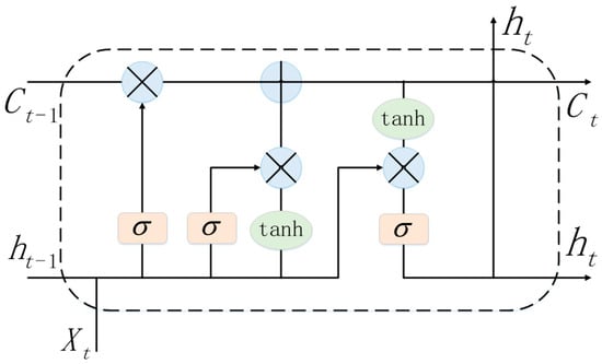
The Long Short-Term Memory network (LSTM) is a specialized recurrent neural network designed to address the vanishing and exploding gradient problems while capturing long-term dependencies in sequential data. Its core innovation lies in a gating mechanism and a persistent cell state that serves as the network’s memory, regulating information flow across extended temporal sequences [24]. Figure 1 illustrates a typical LSTM unit.

Figure 1. Architecture of the LSTM model (based on Hochreiter and Schmidhuber [24]).

The operational principle of LSTM is determined by its gated mechanism, which coordinates memory retention and update through the following mathematical formulation:

$$f_t=\sigma (W_f·[h_{t-1},x_t]+b_f)$$

(1)

$$i_t=\sigma (W_i·[h_{t-1},x_t]+b_i)$$

(2)

$$\widetilde{C_t}=\mathrm{t}\mathrm{a}\mathrm{n}\mathrm{h}(W_C·[h_{t-1},x_t]+b_C)$$

(3)

$${ C}_t=f_t\odot C_{t-1}+i_t\odot \widetilde{C_t}$$

(4)

$$o_t=\sigma (W_o·[h_{t-1},x_t]+b_o)$$

(5)

$$h_t=o_t\odot \mathrm{t}\mathrm{a}\mathrm{n}\mathrm{h}\left(C_t\right)$$

(6)

The forget gate ${ f}_t$ determines the retention of previous memory, the input gate ${ i}_{t }$ and candidate cell state $\widetilde{C_t}$ control the incorporation of new information, and the output gate ${ o}_{t }$ filters the updated cell state to produce the hidden state ${ h}_{t }$. In these equations, $\sigma$ denotes the sigmoid activation function, $\mathrm{t}\mathrm{a}\mathrm{n}\mathrm{h}$ the hyperbolic tangent function, and $⨀$ represents element-wise multiplication. The weight matrices $W_f, W_i, W_C, W_o$ and bias vectors $b_f, b_i, b_C, b_o$ are learnable parameters. This gating mechanism enables the model to leverage relevant historical patterns while adaptively incorporating new observations, making it suitable for capturing complex temporal relationships in multi-parameter water quality time-series data.

3.2. GCN Architecture

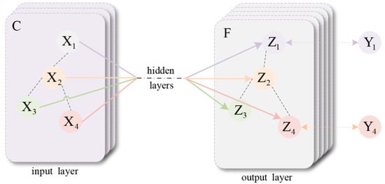
The Graph Convolutional Network (GCN), introduced by Kipf and Welling (2017) and illustrated in Figure 2, is a deep learning method for graph-structured data that performs a localized first-order approximation of spectral graph convolutions [25]. In multi-station water quality monitoring, each station is represented as a node. Edge weights between stations are determined by geographic distance or hydrological connectivity along the river network.

Figure 2. Architecture of the GCN model (based on Kipf and Welling [25]).

Consider a graph G = (V, E) with |V| = S nodes. Let $A\in {\mathbb{R}}^{S\times S }$ be the adjacency matrix and D be the degree matrix with $D_{ii}={\sum }_j{A}_{ij }$. To incorporate each node’s own features, a self-loop is added, yielding $\tilde{A}=A+I_S$, where $I_S$ is the identity matrix. Let $\tilde{D}$ be the corresponding degree matrix with ${\tilde{D}}_{ii}={\sum }_j{\tilde{A}}_{ij}$.

The layer-wise propagation rule of the GCN is then defined as:

$$H^{(l+1)}=\sigma ( {\tilde{D}}^{-{\displaystyle \frac{1}{2}}}\tilde{A}{\tilde{D}}^{-{\displaystyle \frac{1}{2}}}{H}^{\left(l\right)}{W}^{\left(l\right)} )$$

(7)

Here, $H^{\left(l\right)}$ is the node feature matrix at layer l; $W^{\left(l\right)}$ is a trainable weight matrix; and $\sigma (\cdot )$ is a nonlinear activation function. This operation computes a weighted average of the features of a central node and its first-order neighbors, enabling spatial feature smoothing.

3.3. AGConvLSTM Architecture

The Adaptive Graph Convolutional Long Short-Term Memory Network (AGConvLSTM) is the core model proposed in this paper. It integrates graph convolution into the LSTM framework, in contrast to conventional approaches that stack spatial and temporal modules in series. The core of AGConvLSTM is a GraphConvLSTMCell, in which adaptive graph convolution is embedded within the four LSTM gates (input, forget, output, and candidate memory cell). Consequently, spatial information is aggregated at every time step during each gating operation of the memory update.

3.3.1. GraphConvLSTMCell

Let $x_t\in {\mathbb{R}}^{B\times S\times F}$ be the input at time step $t$ and $h_{t-1}\in {\mathbb{R}}^{B\times S\times H}$ the previous hidden state, where B is the batch size, S the number of stations, F the input feature dimension, and H the number of hidden units. First, $x_t$ and $h_{t-1}$ are concatenated along the feature dimension to obtain $c_t=[x_t, h_{t-1}]\in {\mathbb{R}}^{B\times S\times (F+H)}$. Four adaptive graph convolutional layers then process this combined feature to generate the gate activations:

$$i_t=\mathsf{\sigma }\left({\mathrm{G}\mathrm{C}\mathrm{N}}_i\right(c_t)+b_i)$$

(8)

$$f_t=\mathsf{\sigma }\left({\mathrm{G}\mathrm{C}\mathrm{N}}_f\right(c_t)+b_f)$$

(9)

$$o_t=\mathsf{\sigma }\left({\mathrm{G}\mathrm{C}\mathrm{N}}_o\right(c_t)+{\mathrm{b}}_o)$$

(10)

$$\widetilde{C_t}=\mathrm{t}\mathrm{a}\mathrm{n}\mathrm{h}\left({\mathrm{G}\mathrm{C}\mathrm{N}}_c\right(c_t)+b_c)$$

(11)

Here, $\sigma$ denotes the sigmoid activation function, $\mathrm{t}\mathrm{a}\mathrm{n}\mathrm{h}$ is the hyperbolic tangent function, and $b_i, b_f, b_o, b_c$ are bias vectors. The cell state and hidden state are then updated following the standard LSTM rules:

$$C_t=f_t\odot C_{t-1}+i_t\odot \widetilde{C_t}$$

(12)

$$h_t=o_t\odot \mathrm{t}\mathrm{a}\mathrm{n}\mathrm{h}\left(C_t\right)$$

(13)

The key difference from conventional LSTM is that each gating signal is computed via adaptive graph convolution, which aggregates spatial information from all stations. Consequently, the model captures multi-station spatial correlations when forgetting, storing, and outputting information.

3.3.2. Adaptive Graph Convolution

The proposed adaptive graph convolution does not rely on a fixed predefined adjacency matrix. Instead, it learns an adjacency matrix from data, initialized with a geographic prior. A learnable logit matrix $\mathsf{\Theta }\in {\mathbb{R}}^{S\times S}$ is introduced, and the adaptive adjacency matrix is generated via the softmax function:

$$A_{adapt}=softmax\left(\mathsf{\Theta }\right)$$

(14)

A learnable self-loop weight $\alpha$ and a gating factor $\beta$ are also introduced, both constrained to the range (0, 1) via the sigmoid function. The final normalized adjacency matrix is constructed as:

$$\tilde{A}=A_{adapt}+\alpha I_S$$

(15)

$$A_{norm}=\beta \cdot {\tilde{D}}^{-{\displaystyle \frac{1}{2}}}\tilde{A}{\tilde{D}}^{-{\displaystyle \frac{1}{2}}}$$

(16)

where $I_S$ is the identity matrix and $\widetilde{D }$ is the degree matrix of $\tilde{A}$ (${\tilde{D}}_{ii}={\sum }_j{\tilde{A}}_{ij}$). The graph convolution operation is defined as:

$$\mathrm{G}\mathrm{C}\mathrm{N}\left(c\right)=\sigma (A_{norm}\cdot c\cdot W+b)$$

(17)

Here W is a learnable weight matrix and b is the bias vector.

3.3.3. Overall Parameter Configuration

The input data shape is (T, S, F) with T = 12 (time steps), S = 13 (stations), and F = 5 (PCA-reduced features). After batch normalization and a fully connected layer that maps the input to the hidden dimension H = 24, the data are fed into a bidirectional GraphConvLSTMCell. Following temporal attention pooling, residual connection, layer normalization, and dropout, the output is transformed into a 13 × 2 probability distribution. Key hyperparameters are listed in Table 1.

Table 1. Parameter configuration of the AGConvLSTM model.

Component	Parameter	Value
GraphConvLSTMCell	Hidden units	24
	Learnable adjacency matrix	$\mathsf{\Theta } \in {\mathrm{R}}^{13 \times 13}$
	Self-loop weight $\alpha$	Learnable (sigmoid-constrained)
	Gating factor $\beta$	Learnable (sigmoid-constrained)
	L2 regularization coefficient	1 × 10−2
AGConvLSTM	Direction	Forward + backward
Dropout	Dropout rate	0.4

The AGConvLSTM model addresses the limitations of serial spatiotemporal modeling by integrating adaptive graph convolution inside the LSTM gates. It learns dynamic spatial dependencies end-to-end and is specifically designed for multi-station water quality classification.

4. Empirical Analysis

4.1. Study Area and Data Source

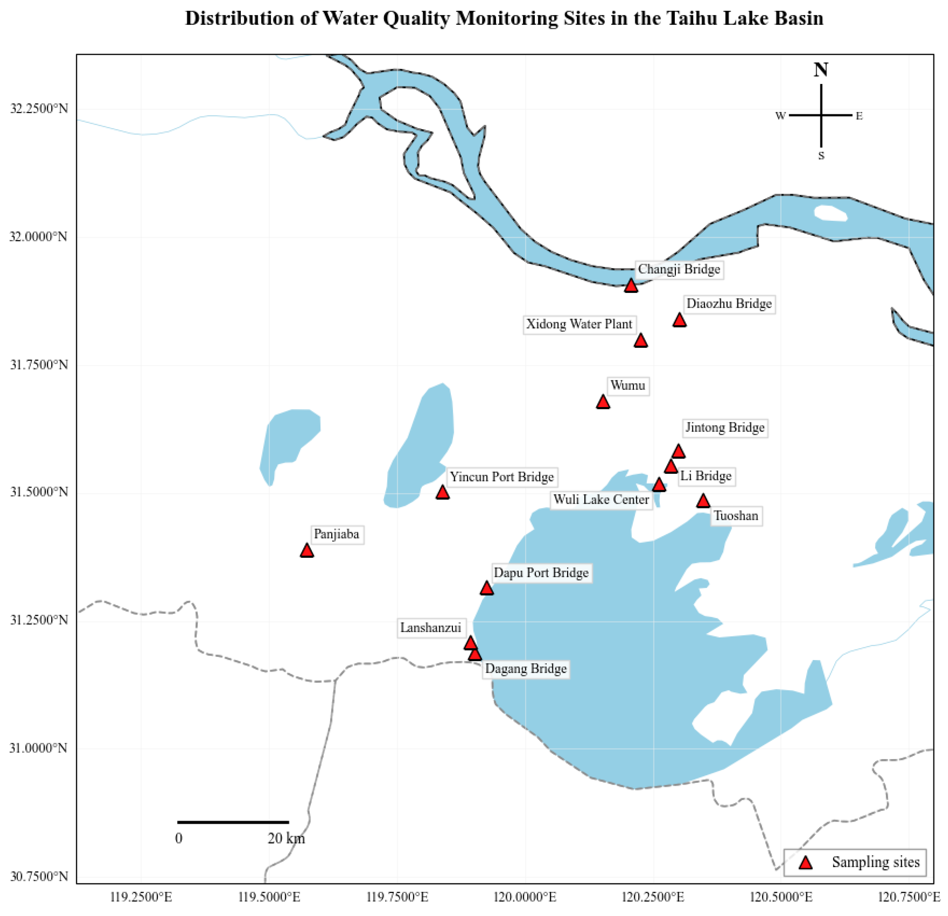
To evaluate the model, a comprehensive dataset was constructed from the Wuxi section of Lake Taihu. It comprises nine water quality parameters collected at 4 h intervals from 13 monitoring stations between May 2020 and May 2025. The data were obtained from the National Surface Water Quality Automatic Monitoring Real-time Data Release System. The monitoring stations include Xidong Water Plant, Lanshanzui, Liqiao, Yincungang Bridge, Dapugang Bridge, Wumu, Tuoshan, Wuli Lake Center, Jintong Bridge, Dagang Bridge, Panjiaba, Changji Bridge, and Diaozhu Bridge. Their spatial distribution is shown in Figure 3. The selected parameters are water temperature (WT), pH, dissolved oxygen (DO), permanganate index (CODMn), ammonia nitrogen (NH₃-N), total phosphorus (TP), total nitrogen (TN), electrical conductivity (EC), and turbidity (NTU). Total phosphorus and total nitrogen are expressed as elemental concentrations. All measurements comply with the Chinese Environmental Quality Standards for Surface Water (GB 3838-2002) [26], with necessary supplements. Table 2 summarizes the standard limits for the parameters relevant to this study.

Figure 3. Distribution of water quality monitoring sites in the Taihu basin.

Table 2. Surface water quality standards (Source: Chinese Environmental Quality Standards for Surface Water [26]).

Water Quality Parameter		Class I	Class II	Class III	Class IV	Class V	Inferior to Class V
Electrical Conductivity ($\mathsf{\mu }$S/cm)	≤	1000	2000	3000	4000	5000	Water quality parameters inferior to Class V
Turbidity (NTU)	≤	3	5	10	20	30
Total Nitrogen (mg/L)	≤	0.2	0.5	1.0	1.5	2.0
Total Phosphorus (mg/L)	≤	0.02	0.1	0.2	0.3	0.4
Ammonia Nitrogen (mg/L)	≤	0.15	0.5	1.0	1.5	2.0
Permanganate Index (mg/L)	≤	2	4	6	10	15
Dissolved Oxygen (mg/L)	≥	7.5	6	5	3	2
pH (dimensionless)		6~9
Water Temperature (°C)	Human-induced water temperature changes are limited to a decrease of 2 °C or an increase of 1 °C in the weekly average maximum temperature.

4.2. Data Preprocessing

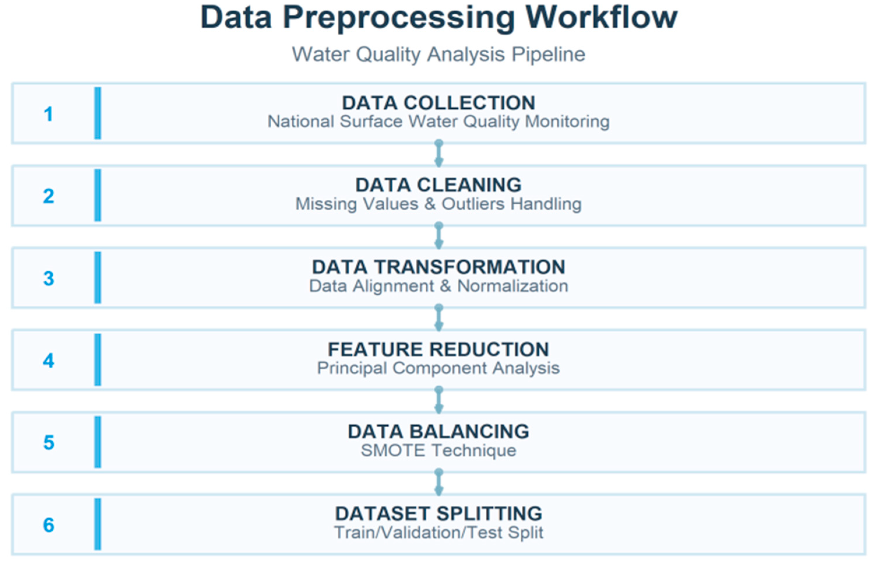
To ensure that data quality satisfies deep learning requirements, the following preprocessing steps were applied: data cleaning and alignment, station-wise PCA dimensionality reduction (from 9 to 5 features), and DTW-SMOTE oversampling with adaptive sampling and dynamic denoising to address class imbalance. The overall workflow is illustrated in Figure 4.

Figure 4. Data preprocessing workflow.

4.2.1. Data Cleaning and Missing Value Imputation

Samples with missing class labels were removed first. For numerical parameters, outliers were detected using the median absolute deviation (MAD) method with a threshold of 6 × MAD and replaced with NaN. A forward fill (limit = 2) was applied within each station, and rows still containing NaN were dropped. To construct a complete spatiotemporal panel (full 4 h grid), a multi-stage imputation procedure was performed: spline interpolation, boundary fill (forward and backward), and global mean imputation as a final option. Class labels were filled using forward or backward fill. After these steps, the panel contained no missing values, with each timestamp covering all stations. The cleaned data were then split into training, validation, and test sets at a ratio of 0.6:0.2:0.2.

4.2.2. DTW-SMOTE with Adaptive Sampling and Dynamic Denoising

The original class distribution was severely imbalanced, which would bias model predictions toward the majority classes. To address this issue, a DTW-SMOTE framework was developed, operating directly in the time-series space rather than relying on Euclidean distance.

(1)

Synthetic sample generation: For each minority class, pairwise dynamic time warping (DTW) distances were computed using the fastdtw library. For each sample, its k = 3 nearest neighbors were identified based on DTW distance. A synthetic sample was generated as:

$$x_{\mathrm{new}}=x_i+\alpha · (x_j -{ x}_i) \alpha \sim \mathrm{U}(0,1)$$

(18)

where $x_j$ is a randomly chosen DTW neighbor of $x_i$.

(2)

Adaptive sampling: Instead of oversampling all minority classes to a uniform size, class-pairwise Mahalanobis distances were computed in the feature space. Classes with smaller pairwise distances received larger oversampling boosts. The target count for each class was set as:

$${target}_c=min(majority\times 0.5,\hspace{1em}{original}_c\times {boost}_c)$$

(19)

where the boost factor for each class was determined from the distance matrix and a confusion percentile threshold (the 30th percentile).

(3)

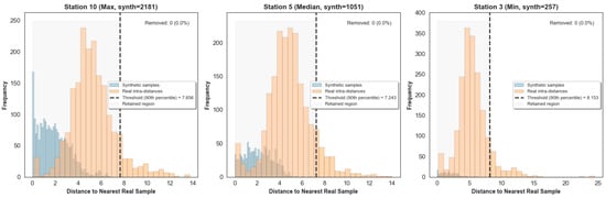
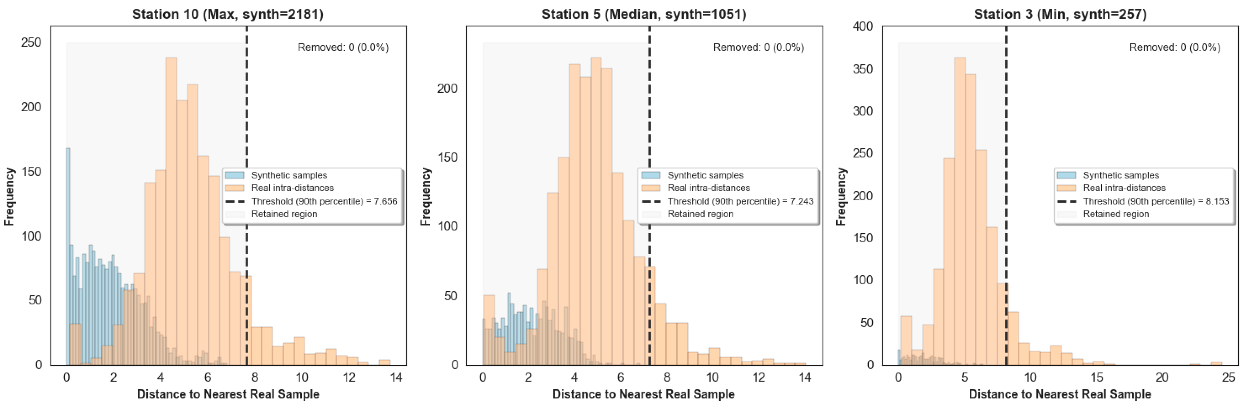
Dynamic denoising: After generating synthetic samples, each synthetic sample’s Euclidean distance to its nearest real sample was computed. The 90th percentile of distances from real samples to their nearest neighbors within the same class was used as a threshold. Synthetic samples with distances exceeding this threshold were discarded, effectively removing outliers that could blur class boundaries. Figure 5 illustrates the distance distributions and the filtering effect for three representative stations (with the maximum, median, and minimum numbers of synthetic samples). Synthetic samples with distances above the 90th percentile threshold were removed.

Figure 5. Distance distributions of synthetic samples to nearest real samples for three representative stations.

(4)

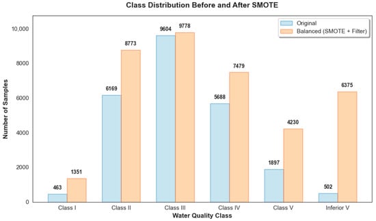
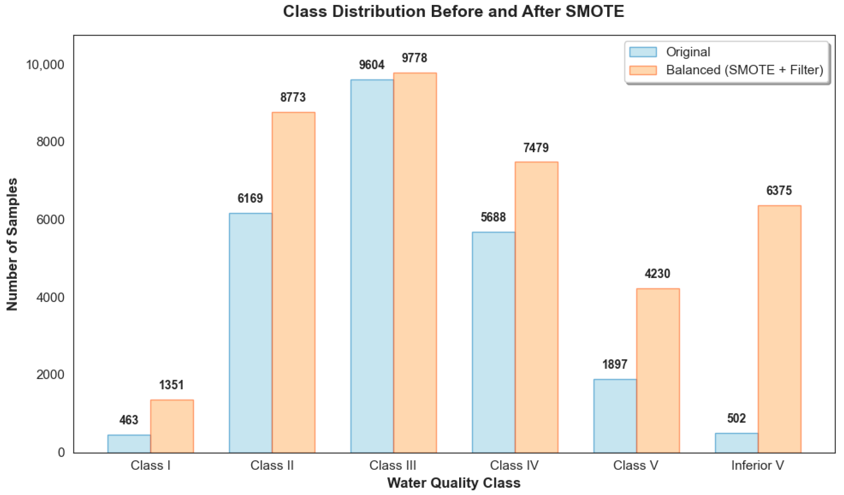
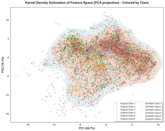
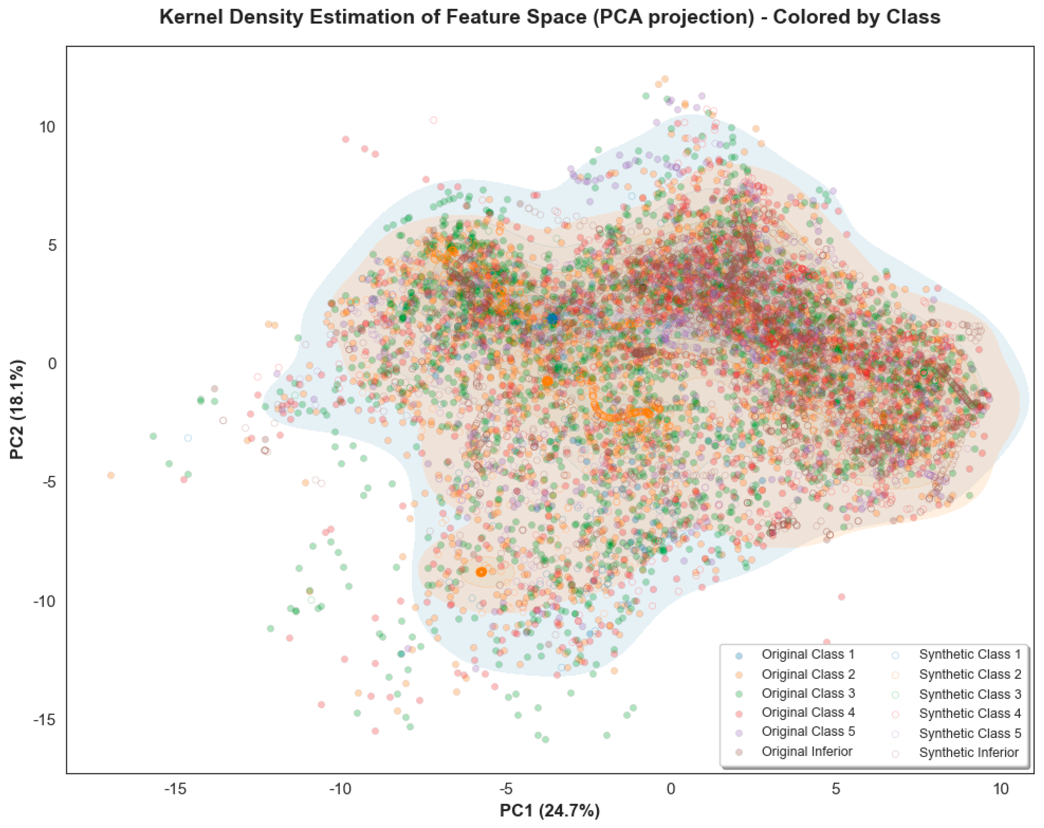
Final alignment: After applying the above steps independently to each of the 13 stations, the number of synthetic samples per station varied. The median count (1051) was chosen as the target, and all stations were aligned to this number through random sampling or light oversampling with small additive noise. The final balanced training set contained 2922 samples (originally 1871). The class distributions before and after balancing are shown in Figure 6. Additionally, Figure 7 presents the kernel density estimation of original and synthetic samples in the PCA-transformed feature space, confirming that the generated samples populate the same regions as the real ones.

Figure 6. Class distribution before and after balancing.

Figure 7. Kernel density estimation of feature space.

4.2.3. Station-Wise PCA for Dimensionality Reduction

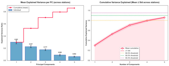
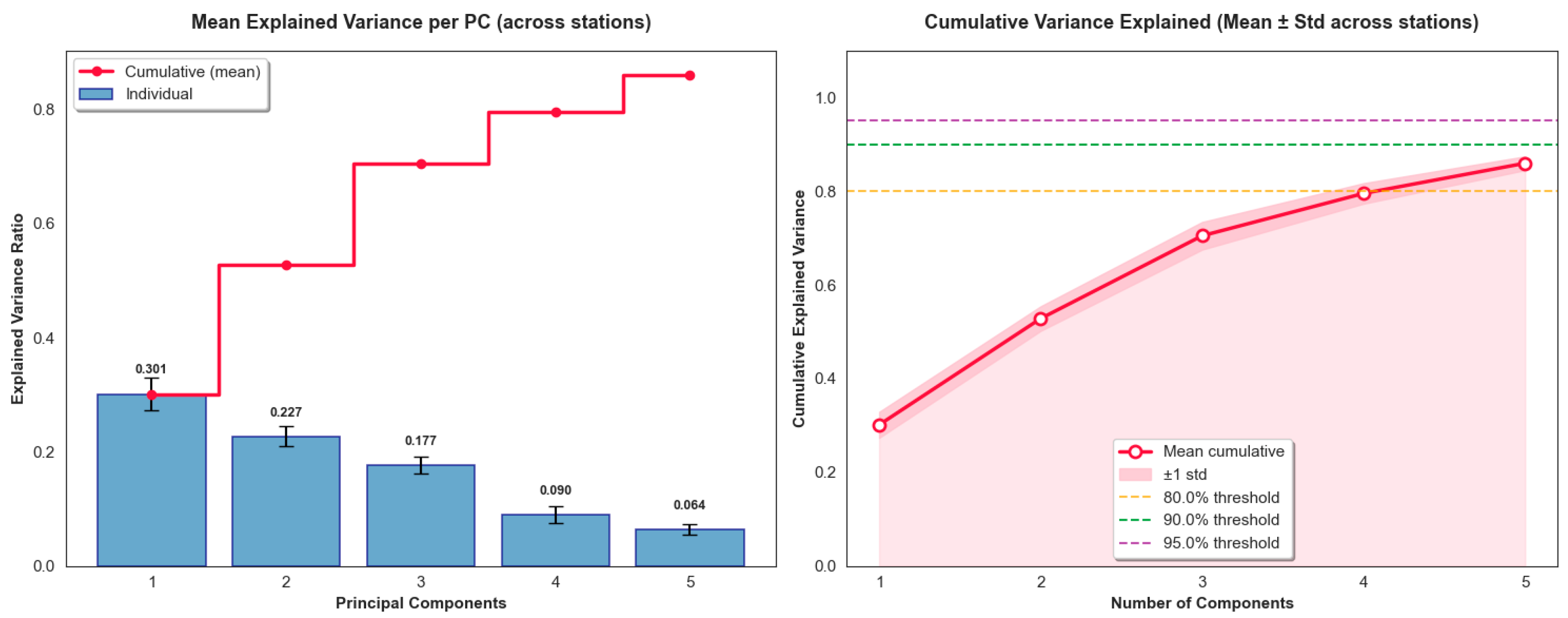
Conventional global PCA applies the same principal components to all stations, overlooking spatial heterogeneity. Instead, station-wise PCA was applied to each of the 13 stations: a separate PCA model was fitted on the standardized 9-dimensional feature vectors of each station. The first five principal components (PC1-PC5) were retained per station, reducing the feature dimension from 9 to 5. Across stations, the cumulative variance explained by PC1-PC5 ranged from 82% to 88% (mean = 85.96%). Figure 8 presents the per-component and cumulative explained variance.

Figure 8. Per-component and cumulative explained variance.

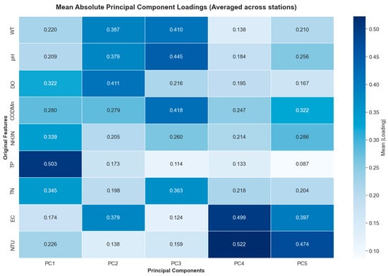
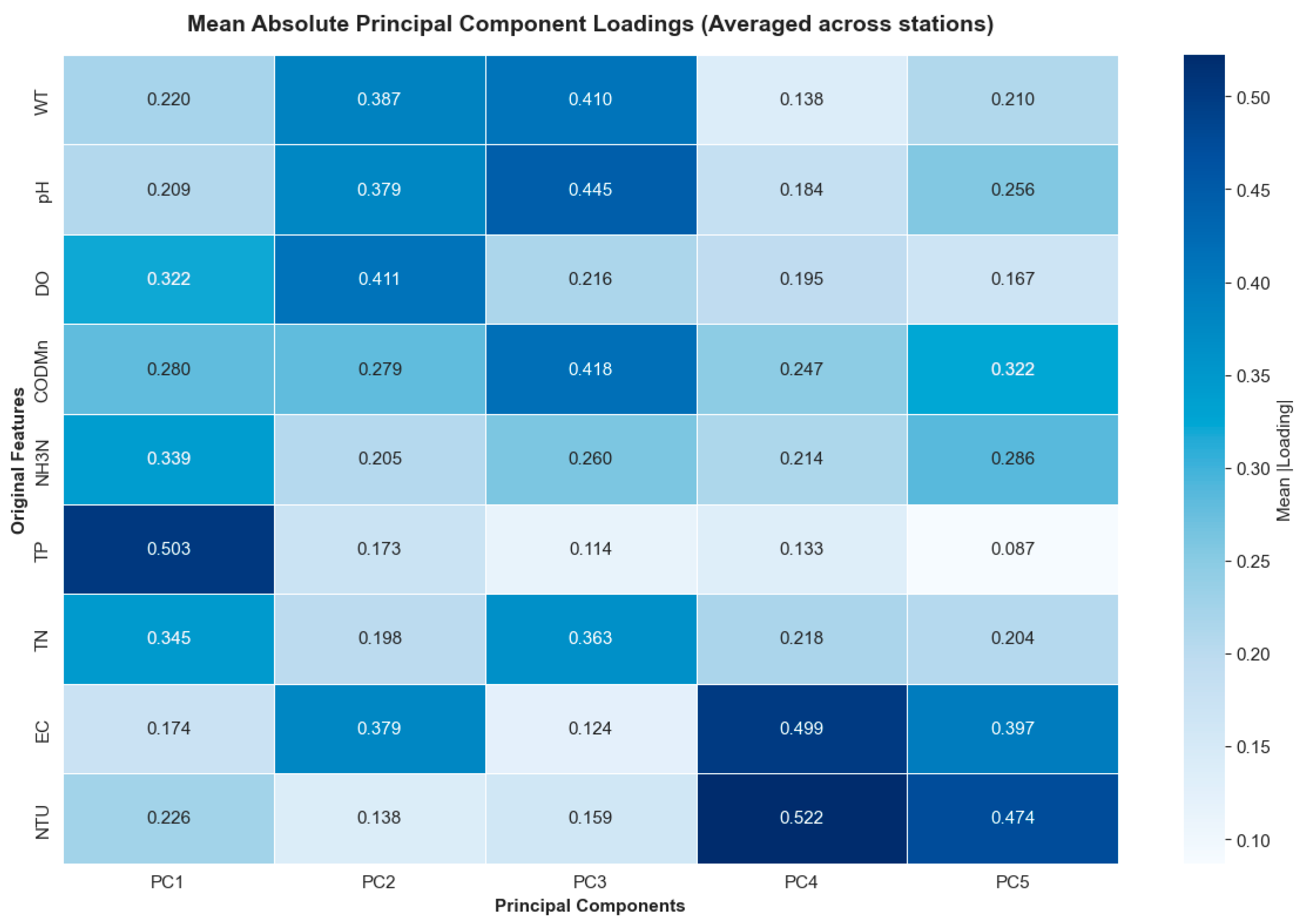
Figure 9 presents the mean absolute loadings across all stations. The analysis reveals that PC1 is dominated by nutrient-related parameters (NH₃-N, TP, TN), reflecting pollution loading; PC2 is mainly determined by dissolved oxygen (DO), water temperature (WT), pH, and electrical conductivity (EC), collectively representing the physicochemical environment; PC3 is primarily associated with permanganate index (CODMn), water temperature (WT), and pH, indicating organic pollution and seasonal variations. In summary, station-wise PCA not only reduces the feature dimension from 9 to 5 but also respects the spatial heterogeneity of water quality patterns across monitoring stations in Lake Taihu, avoiding the information loss caused by a single global transformation. This method provides a low-dimensional input that preserves local hydrological signatures for subsequent spatiotemporal classification models.

Figure 9. Mean absolute principal component loadings.

4.3. Model Performance

4.3.1. Model Training Design

The AGConvLSTM model was trained on the balanced dataset (2922 samples) derived after station-wise PCA and DTW-SMOTE preprocessing. A binary classification task was defined to align with water quality management needs: the original six classes (Class I to Inferior to Class V) were merged into two categories: “compliant” (Class 0), comprising Classes I, II, and III, and “non-compliant” (Class 1), comprising Classes IV, V, and Inferior to Class V. This grouping follows the Chinese surface water quality standard GB 3838-2002, where Classes I-III indicate water bodies meeting the national quality targets, whereas Classes IV-V and Inferior to Class V represent progressively elevated pollution levels. After merging, the two classes achieved a balanced distribution in the training set, mitigating class imbalance.

All models were implemented using Python 3.11.9, TensorFlow 2.20.0, NumPy 2.3.3, and Pandas 2.3.3. The same random seed (42) was used for reproducibility. Training hyperparameters are listed in Table 3.

Table 3. Training hyperparameters.

Hyperparameter	Value
Optimizer	AdamW (β1 = 0.9, β2 = 0.999)
Loss function	Weighted categorical crossentropy
Learning rate	0.0005
Weight decay	1 × 10−4
Gradient clipping norm	1.0
Batch size	256
Maximum epochs	100
L2 regularization coefficient	1 × 10−2

4.3.2. Classification Performance

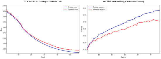
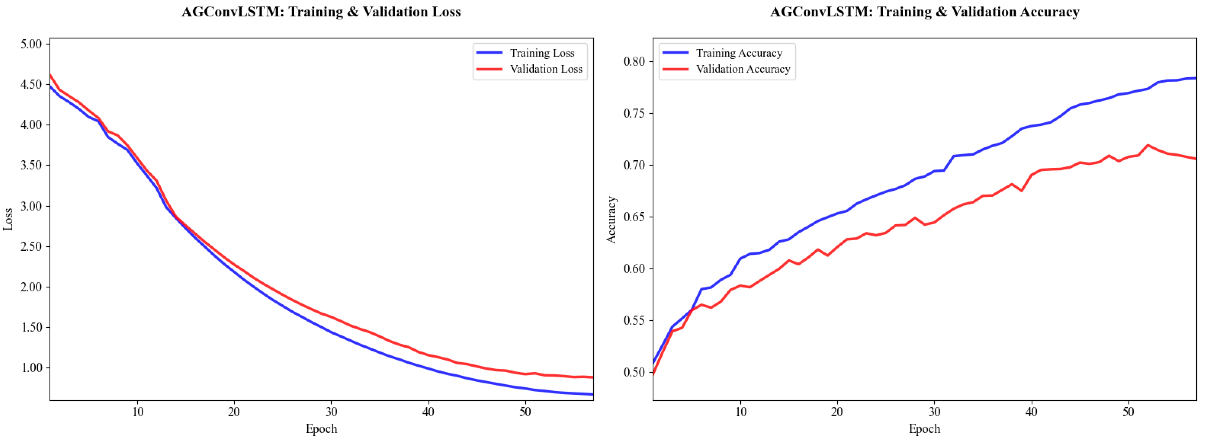
The AGConvLSTM model was trained following the hyperparameters described above. Figure 10 illustrates the training loss and accuracy curves. The training loss decreases smoothly and converges, while the validation accuracy improves in tandem with the training accuracy, indicating good generalization.

Figure 10. Training loss (left) and accuracy (right) curves of the AGConvLSTM model.

The model was evaluated on an independent test set of 625 samples. AGConvLSTM achieved an overall accuracy of 69.34% and an F1 score of 69.68%. However, performance varies substantially across the 13 monitoring stations, reflecting the spatial heterogeneity of water quality in Lake Taihu.

Table 4 summarizes the classification performance of five representative stations. Among them, Lanshanzui achieves the highest accuracy (88.48%) and F1 (85.85%). Notably, for stations such as Lanshanzui and Dagang Bridge, high accuracy aligns well with the F1 score, indicating balanced performance. For other stations, the gap between accuracy and F1 reflects the impact of class imbalance. These results demonstrate that AGConvLSTM can capture station-specific temporal dynamics, but its effectiveness varies with local water quality characteristics, and class imbalance remains a challenge for certain stations.

Table 4. Classification results of representative stations.

Station Name	Accuracy (%)	F1-Score (%)
Lanshanzui	88.48	85.85
Dagang Bridge	85.12	85.19
Liqiao	76.16	69.63
Dapugang Bridge	65.76	66.46
Xidong Water Plant	49.12	51.69

4.4. Comparative Analysis

To evaluate the proposed AGConvLSTM, we compare it against three baseline models: LSTM-AGCN, TCN-AGCN, and ST-AGCN. All four models share the same adaptive graph convolution for spatial modeling, ensuring a fair comparison of temporal processing strategies. The three baselines represent distinct spatiotemporal fusion paradigms: LSTM-AGCN follows a spatial-then-temporal serial design, applying graph convolution first and then a bidirectional LSTM; TCN-AGCN follows a temporal-then-spatial design, extracting temporal features via temporal convolutional networks before graph convolution; and ST-AGCN uses a stacked-block architecture that alternates between temporal and spatial processing. In contrast, AGConvLSTM couples spatial and temporal information by embedding graph convolution inside the LSTM gates. Thus, comparing AGConvLSTM with these baselines highlights the advantage of deep spatiotemporal fusion over conventional serial or stacked designs. All models were trained and tested under identical conditions (same data split, batch size, optimizer, and early stopping). Table 5 summarizes their overall performance on the test set in terms of accuracy, precision, and F1 score.

Table 5. Comparison of model performance metrics.

Model	Accuracy (%)	Precision (%)	F1-Score (%)
AGConvLSTM	69.34	70.19	69.68
LSTM-AGCN	61.40	66.65	62.48
TCN-AGCN	60.25	66.34	61.34
ST-AGCN	63.36	69.69	64.36

AGConvLSTM consistently outperformed all three baseline models across every evaluation metric. Compared to the second-best model (ST-AGCN), it achieved improvements of 5.98% in accuracy, 0.50% in precision, and 5.32% in F1. The largest gains were observed against TCN-AGCN, with increases of 9.09% in accuracy, 3.85% in precision, and 8.34% in F1. These results demonstrate that the deep spatiotemporal fusion strategy of AGConvLSTM, embedding adaptive graph convolution inside the LSTM gates, is more effective for multi-station water quality classification than serial (LSTM-AGCN, TCN-AGCN) or stacked-block (ST-AGCN) architectures.

5. Discussion and Conclusions

5.1. Superiority of AGConvLSTM

AGConvLSTM outperformed all baseline models across all evaluation metrics. Its advantage stems from a deep spatiotemporal coupling design: each LSTM gate (input, forget, output, candidate) receives spatial information via graph convolution at every time step, allowing the model to adjust memory and output based on current spatial dependencies. In contrast, LSTM-AGCN applies graph convolution only once per step before the LSTM, TCN-AGCN extracts temporal features first and adds spatial aggregation at the end, and ST-AGCN processes time and space in separate stacked blocks. These designs either fail to refresh spatial information during temporal updates or limit real-time interaction.

Compared with recent graph-based multi-station models, STF-GNN [7] integrates GCN, GRU, and self-attention to capture multi-scale dependencies, while W-WaveNet [8] stacks adaptive graph convolution and CNN-LSTM. Both models process spatial and temporal information in distinct modules. AGConvLSTM differs by fusing graph convolution inside LSTM gates, achieving tighter spatiotemporal integration.

Compared with non-spatiotemporal models such as PCA-BP [12], both methods use oversampling to handle class imbalance. PCA-BP applies standard SMOTE, while AGConvLSTM employs DTW-SMOTE, which preserves temporal similarity. After SMOTE balancing, PCA-BP reached 94.52% accuracy on a single-station dataset. AGConvLSTM achieved 69.34% test accuracy on a multi-station dataset balanced via DTW-SMOTE. The difference reflects the higher complexity of the multi-station task.

5.2. Practical Implications and Limitations

The AGConvLSTM model provides practical support for water quality management in Lake Taihu. First, it enables early warning of non-compliant events by processing real-time 4 h data and identifying stations that are predicted to fall below Class III. Second, the substantial performance gap between stations suggests reallocating monitoring resources: increase sampling frequency or add parameters at low-performing stations. Third, the DTW-SMOTE framework offers a methodological reference for other imbalanced environmental classification tasks.

Despite these practical benefits, several limitations must be acknowledged.

First, generalization limitations. The model has not been validated on independent data from other time periods or geographic locations. In contrast, STF-GNN [7] and W-WaveNet [8] have been evaluated on multiple river network datasets, demonstrating cross-basin generalization. Our model’s transferability to other lakes or river networks remains unknown.

Second, computational cost. The GraphConvLSTMCell increases training time due to four adaptive graph convolutions per time step. While inference remains fast, this cost is higher than that of a standard LSTM and comparable to other spatiotemporal graph models.

Third, class imbalance and initialization bias. Even after DTW-SMOTE, some stations still show a gap between accuracy and F1 scores, indicating that class imbalance is not fully resolved. Additionally, the adaptive adjacency matrix is initialized using a geographic distance prior, which may bias learning toward spatial proximity.

5.3. Conclusions and Future Work

This study proposes AGConvLSTM, a deep learning model for multi-station water quality classification, validated on a five-year dataset from 13 stations in Lake Taihu. The main contributions are threefold.

First, a deep spatiotemporal fusion architecture is developed. AGConvLSTM embeds adaptive graph convolution inside the LSTM gates, achieving tighter space–time coupling. Second, a DTW-SMOTE framework with adaptive sampling and dynamic denoising is introduced for time-series water quality data, effectively mitigating class imbalance. Third, a station-wise independent PCA strategy replaces global PCA, preserving local feature structures across stations and respecting spatial heterogeneity.

AGConvLSTM achieves a test accuracy of 69.34% and an F1 score of 69.68%, yet station-wise accuracy varies substantially, reflecting strong spatial heterogeneity. Nonetheless, the limitations discussed above remain.

Future work will focus on the following directions. First, transfer learning will be applied to other lakes or river basins to test generalizability. Second, integrating physical constraints may improve interpretability and robustness. Third, advanced generative models such as TimeGAN will be explored to replace DTW-SMOTE for producing higher-quality synthetic samples. Fourth, edge deployment will enable real-time on-site early warning. Fifth, explainability analysis, such as attention visualization, will reveal which stations and time steps most influence classification decisions.

References

- Frincu, R.M. Artificial intelligence in water quality monitoring: A review of water quality assessment applications. Water Qual. Res. J. 2025, 60, 164–176. [Google Scholar] [CrossRef] [Scilit]
- Muñoz-Alegría, J.A.; Núñez, J.; Oyarzún, R.; Chávez, C.A.; Arumí, J.L.; Rodríguez-López, L. A bibliometric-systematic literature review (B-SLR) of machine learning-based water quality prediction: Trends, gaps, and future directions. Water 2025, 17, 2994. [Google Scholar] [CrossRef] [Scilit]
- He, M.; Qian, Q.; Liu, X.; Zhang, J.; Curry, J. Recent progress on surface water quality models utilizing machine learning techniques. Water 2024, 16, 3616. [Google Scholar] [CrossRef] [Scilit]
- Oğuz, A.; Ertuğrul, Ö.F. A survey on applications of machine learning algorithms in water quality assessment and water supply and management. Water Supply 2023, 23, 895–922. [Google Scholar] [CrossRef] [Scilit]
- Ramya, S.; Srinath, S.; Tuppad, P. Comprehensive analysis of multiple classifiers for enhanced river water quality monitoring with explainable AI. Case Stud. Chem. Environ. Eng. 2024, 10, 100822. [Google Scholar] [CrossRef] [Scilit]
- Zhang, M.; Zhang, Z.; Wang, X.; Liao, Z.; Wang, L. The use of attention-enhanced CNN-LSTM models for multi-indicator and time-series predictions of surface water quality. Water Resour. Manag. 2024, 38, 6103–6119. [Google Scholar] [CrossRef] [Scilit]
- Wan, H.; Xiang, L.; Cai, Y.; Xie, Y.; Xu, R. Temporal and spatial feature extraction using graph neural networks for multi-point water quality prediction in river network areas. Water Res. 2025, 281, 123561. [Google Scholar] [CrossRef] [Scilit]
- Yang, S.; Zhong, S.; Chen, K. W-WaveNet: A multi-site water quality prediction model incorporating adaptive graph convolution and CNN-LSTM. PLoS ONE 2024, 19, e0276155. [Google Scholar] [CrossRef] [Scilit] [PubMed]
- Li, P.; Zhu, Z. STGCN-WQ: A new spatio-temporal graph convolutional network for predicting beach water quality. Environ. Model. Softw. 2026, 195, 106731. [Google Scholar] [CrossRef] [Scilit]
- Akash, P.V.; Babu, N.V. Feature-optimized multiclass water quality detection in Kerala’s medium minor rivers using Siamese networks. In Proceedings of the 2025 International Conference on Advances in Modern Age Technologies for Health and Engineering Science (AMATHE), Shivamogga, India, 24–25 April 2025. [Google Scholar] [CrossRef] [Scilit]
- Sangwan, V.; Bhardwaj, R. Machine learning framework for predicting water quality classification. Water Pract. Technol. 2024, 19, 4499–4521. [Google Scholar] [CrossRef] [Scilit]
- Gao, M.; Qian, Y.; Zhang, Q.; Liu, Y.; Zhang, Z. Surface water quality classification and prediction model based on multiple machine learning algorithms. Sci. Rep. 2025, 15, 39907. [Google Scholar] [CrossRef] [Scilit]
- Pyo, J.C.; Pachepsky, Y.; Kim, S.; Abbas, A.; Kim, M.; Kwon, Y.S.; Ligaray, M.; Cho, K.H. Long short-term memory models of water quality in inland water environments. Water Res. X 2023, 21, 100207. [Google Scholar] [CrossRef] [Scilit]
- Zhang, Q.; Wang, R.; Qi, Y.; Wen, F. A watershed water quality prediction model based on attention mechanism and Bi-LSTM. Environ. Sci. Pollut. Res. 2022, 29, 75664–75680. [Google Scholar] [CrossRef] [Scilit]
- Zamani, M.G.; Nikoo, M.R.; Jahanshahi, S.; Barzegar, R.; Meydani, A. Forecasting water quality variable using deep learning and weighted averaging ensemble models. Environ. Sci. Pollut. Res. 2023, 30, 124316–124340. [Google Scholar] [CrossRef] [Scilit]
- Achuthankutty, S.; Padma, M.; Deiwakumari, K.; Kavipriya, P.; Prathipa, R. Deep learning empowered water quality assessment: Leveraging IoT sensor data with LSTM models and interpretability techniques. Int. J. Comput. Exp. Sci. Eng. 2024, 10, 731–743. [Google Scholar] [CrossRef] [Scilit]
- Nasaruddin, N.; Masseran, N.; Idris, W.M.R.; Ul-Saufie, A.Z. A SMOTE PCA HDBSCAN approach for enhancing water quality classification in imbalanced datasets. Sci. Rep. 2025, 15, 13059. [Google Scholar] [CrossRef] [Scilit] [PubMed]
- Yu, Z.; Song, L.; Zhou, E.; Li, H.; Zhang, J.; Lin, H. Machine learning framework and spatiotemporal variation analysis for water quality classification in the Xiangjiang basin. In The International Conference on Computer Vision and Deep Learning (CVDL 2024); Association for Computing Machinery: New York, NY, USA, 2024. [Google Scholar] [CrossRef] [Scilit]
- Shehab, S.A.; Darwish, A.; Hassanien, A.E. Water quality classification model with small features and class imbalance based on Fuzzy Rough Sets. Environ. Dev. Sustain. 2025, 27, 1401–1419. [Google Scholar] [CrossRef] [Scilit]
- Lokman, A.; Wan Ismail, W.Z.; Ab Aziz, N.A. A review of water quality forecasting and classification using machine learning models and statistical analysis. Water 2025, 17, 2243. [Google Scholar] [CrossRef] [Scilit]
- Guigues, N.; Desenfant, M.; Hance, E. Combining multivariate statistics and analysis of variance to redesign a water quality monitoring network. Environ. Sci. Process. Impacts 2013, 15, 1692–1705. [Google Scholar] [CrossRef] [Scilit]
- Gutiérrez, K.; Lischeid, G.; Rode, M. Disentangling spatiotemporal water quality dynamics in a heterogeneous catchment using high-frequency data and principal component analysis. In Proceedings of the European Geosciences Union General Assembly 2025 (EGU25), Vienna, Austria, 27 April–2 May 2025; p. EGU25-3542. [Google Scholar] [CrossRef] [Scilit]
- Zhi, W.; Appling, A.P.; Golden, H.E.; Podgorski, J.; Li, L. Deep learning for water quality. Nat. Water 2024, 2, 228–241. [Google Scholar] [CrossRef] [Scilit]
- Hochreiter, S.; Schmidhuber, J. Long short-term memory. Neural Comput. 1997, 9, 1735–1780. [Google Scholar] [CrossRef] [Scilit] [PubMed]
- Kipf, T.N.; Welling, M. Semi-supervised classification with graph convolutional networks. In Proceedings of the International Conference on Learning Representations (ICLR 2017), Toulon, France, 24–26 April 2017. [Google Scholar] [CrossRef] [Scilit]
- GB 3838-2002; Environmental Quality Standards for Surface Water. China Environmental Science Press: Beijing, China, 2002.
Disclaimer/Publisher’s Note: The statements, opinions and data contained in all publications are solely those of the individual author(s) and contributor(s) and not of MDPI and/or the editor(s). MDPI and/or the editor(s) disclaim responsibility for any injury to people or property resulting from any ideas, methods, instructions or products referred to in the content. |
© 2026 by the authors. Licensee MDPI, Basel, Switzerland. This article is an open access article distributed under the terms and conditions of the Creative Commons Attribution (CC BY) license.