


Abstract
Given that flood disasters often occur in areas without sufficient instrumentation, conventional observation networks alone may be inadequate to capture the actual evolution of flood events. However, video content from diverse sources such as smartphones, dashboard cameras, surveillance cameras, and helicopters or drones used for rescue, reconnaissance, or reporting, are increasingly collected incidentally and are gaining attention as complementary sensing modalities. Quasi-viewpoint fixation is key to quantitative hydraulic measurements because such videos involve significant changes in their point of view over the course of a given clip. To this end, we developed a quasistatic stabilization technique for social sensing referred to as QS4. The results of a laboratory experiment show that QS4 reproduced velocity distributions comparable to those of a fixed camera for pan-dominant videos recorded with a moving camera. In the 2024 Tsukada River flood, QS4 yielded stable velocity fields despite high turbidity, driftwood, and partial occlusions. Following the blockage of a bridge, flows were detoured along buildings shifting from a channel to flow through farmland, where ~5 m/s flows caused building failures that could not be detected by fixed observations. QS4 offers a practical pathway for transforming incidental videos into quantitative hydraulic observations.
1. Introduction
In recent years, with the progression of climate change, heavy rainfall disasters have intensified and become more frequent worldwide [1,2,3,4]. Notable large-scale flood disasters include the 2022 Pakistani and 2023 Storm Daniel floods. During the 2022 floods in Pakistan, abnormal rainfall was induced by moisture transport from two atmospheric rivers passing over southern Pakistan, resulting in the evacuation of ~32 million people as well as significant mortality (~1500 human lives) [5]. The impacts of Storm Daniel in 2023 will extend across numerous countries, including Greece, Türkiye, Bulgaria, and Libya, where approximately 5923 deaths are expected to result from dam failures [6]. Many such extreme rainfall events are amplified by warm sea surface conditions, and their intensity and frequency are projected to increase with climate change [7,8]. Consequently, rising river water levels and discharge are of increasing concern along with expanding inundation from flooding [9,10,11].
Clarifying flow phenomena in rivers and inundation zones during extreme flood conditions is essential for designing and implementing both structural and nonstructural measures for extreme floods [12,13]. This includes investigating the spatiotemporal variability in water level, depth, velocity, and discharge. In addition to the flow within river channels, elementary flow processes in inundated areas, where direct human and physical damage occurs, are critically important [14,15]. For water-level observations, affordable internet of things (IoT) sensors, non-contact sensors based on computer vision and radar, and satellite-based aerial measurements are advancing [16,17,18]. For velocity measurements, which are necessary for discharge estimation, various instruments are used: classical point-velocity meters, such as propeller and electromagnetic current meters [19,20], acoustic Doppler current profiler (aDcp) systems [21,22], and horizontal (H)-aDcp systems [23,24,25] which can measure vertical and lateral profiles. Other options include microwave current meters that enable stable automatic continuous observations [26,27] and image processing methods that compute velocity distributions from camera images of the river surface [28,29,30]. Many of these methods have been practically applied in this field. However, their maturity, accuracy, and applicability are not equivalent. In particular, conventional in situ methods, such as propeller current meters and aDcp-based systems, are relatively mature and can provide reliable observations under appropriate deployment conditions. By contrast, image-based approaches, especially those using natural river-surface videos without tracers, may be more sensitive to hydraulic and imaging conditions, and their reliability may therefore be lower in some cases. At the same time, even well-established conventional systems are often costly and require substantial preparation and planning for field deployment, making it difficult to maintain sufficiently dense observations in all rivers and inundation areas. This suggests the importance of developing complementary observational approaches, together with the continued improvement of conventional monitoring systems.
Among these velocity measurement modalities, image-based methods that enable non-contact measurements are attracting attention because of their relatively low cost and their practical advantages for flood observations, including improved operator safety and a lower risk of direct sensor damage from high flows and floating debris [31]. In river flow applications, where discharge observation is often the primary objective, cameras are typically fixed on levee crests or banks to record oblique views [29]. The acquired images were geometrically corrected and mapped onto a plane coordinate system before applying the velocimetric algorithms. Common algorithms include large-scale particle image velocimetry (LSPIV) for planar velocity fields [28,30,32], space-time image velocimetry (STIV) for one-dimensional velocity profiles on a cross-section [29,33], and space-time volume velocimetry (STVV), which extends STIV to produce planar two-dimensional velocities [34]. Furthermore, studies using images captured by uncrewed aerial vehicles (UAVs) for image velocimetry are active [35,36,37,38]. As UAV images cannot be perfectly viewpoint-fixed, image stabilization is indispensable. Stabilization has also been applied to fixed cameras subjected to wind-induced shake [39]. The proposed stabilization process tracks static reference points or features in the image, either manually or automatically, to stabilize the video [35,40,41]. When UAV images are not orthoimages, orthorectification using ground control points (GCPs) is commonly performed, followed by adjustments to image contrast and related parameters [30].
Thus, a variety of instruments for measuring flow velocity in river environments have been implemented, and image-based methods, in particular, are rapidly advancing in both software and hardware applications. In contrast, in inundation zones, installing these velocity meters is unrealistic; measurement cases specifically aimed at flooding flows are virtually nonexistent. Meanwhile, numerous instances exist in which flood flows and disaster conditions are recorded by various camera devices for purposes other than hydrometric observation; for example, residents filming flood scenes with smartphones, or in-vehicle dashboard cameras recording conditions as vehicles traverse inundated zones. With the widespread use of cameras, still images and videos are routinely captured, uploaded, or shared on social media [42,43,44]. In parallel with these developments, citizen science has also become an important framework for public participation in environmental and disaster-related data collection and interpretation, and citizen-sensing activities have increasingly been discussed in connection with disaster management and mobile crowdsensing [45,46,47]. Integrated frameworks have also been proposed to combine citizen-contributed information, authoritative observations, and hydrodynamic modelling; for example, the RiverCure Portal provides a Web GIS platform for flood-risk management, and its later extension explicitly incorporates citizen-science functions for collecting field data and promoting public engagement [48,49]. For event-scale flood mapping, methods that map geo-tagged images posted on social media to estimate inundation extents have been proposed [43,50], whereas other studies have combined social media photographs of inundation with SAR imagery and digital elevation models to improve inundation mapping accuracy [51,52]. Text analysis from Weibo combined with image analysis from TikTok was used to map approximate inundation depths by comparing object dimensions with the observed submergence [53]. Deep learning has also been applied to crowdsourced flood photographs for flood detection and severity assessment; for example, Pereira et al. showed that convolutional neural networks can classify flood evidence and severity from social-media photos and complement other information sources such as satellite imagery [54]. While most prior studies targeted the extent of inundation and used highly simplified depth estimation, Chaudhary et al. proposed a deep learning–based method that infers water depth from the submerged state of objects in images and applied it to social media images [55]. LSPIV has also been applied to river flow videos on YouTube to estimate velocity and discharge [56].
In the present study, we use the term social sensing in a broader practical sense. More specifically, while social sensing overlaps with citizen-sensing activities and may include citizen-science-oriented contributions, it is not restricted to citizens alone. Rather, it refers more broadly to the generation and sharing of socially embedded observations by diverse actors, including residents, river administrators, media organizations, emergency responders, and other stakeholders who may capture useful information during disasters.
Although the use of citizen-captured imagery and videos for flood investigations is increasing, there are still no applications for reconstructing flooding flow velocity distributions. This is majorly because, contrary to survey cameras (except security cameras), recording cameras are not fixed, and their viewpoints change substantially. In practice, numerous videos span the surroundings or are recorded while the videographer is moving. To handle such videos, static stabilization must be applied, as noted above, to fix the image viewpoint before geometric correction and velocity analysis. However, robust static stabilization for large viewpoint changes has not yet been established; consequently, velocity analysis for such videos has not been performed. Moreover, images may not conveniently include sufficient GCPs for velocity retrieval; if GCPs lie outside the field of view, applying image velocimetry becomes difficult or inaccurate.
Accordingly, this study aims to develop an image processing technique that yields stable and accurate surface velocity distributions, even for videos with large viewpoint changes recorded by non-hydrometric observers (e.g., residents). This technique involves static stabilization, orthorectification, and flow analysis. For static stabilization, we built a quasi-static stabilization technique for social sensing (QS4) that generalizes prior automatic stabilization techniques [34,35] to handle dynamically changing viewpoints (pan, tilt, and rotation) in arbitrary directions. The stabilized result was projected onto a horizontal plane using an orthorectification technique, and the surface velocities of the flooding flow were estimated based on the optical flow [57]. To verify the basic performance, we conducted laboratory experiments on an open-channel flow to quantify the errors at each step and assess the overall effectiveness. Next, we analyzed videos captured by residents during the huge floods caused by the 2024 Noto Peninsula heavy rains [58] and then evaluated the velocity distributions. Many of these videos recorded the surroundings over approximately 10 s while panning, tilting, and rotating, which aligns well with the applicability conditions of the proposed method. The research questions were considered are presented as follows.
How can the viewpoint of videos that include large movements in the position of the camera be fixed to enable estimation of flow velocity equivalent to what would be possible with a fixed camera?
Can a method for estimating the flow velocity using video recordings captured by residents serve as a complementary approach to existing fixed observation methods?
The novelty of this study lies in estimating planar velocity fields from videos not intended for hydrometric observation that contain pronounced viewpoint motions—pan, tilt, and rotation—through robust viewpoint stabilization. In addition, our approach lies not only in the overall QS4 package, which stably enables velocity estimation for videos with large viewpoint changes, but also in optimizing QS4 specifically for velocity estimation.
2. Materials and Methods
2.1. Target Images and Framework of the Present Image Processing Methods
We targeted videos with large viewpoint changes recorded by residents and others and performed image-based velocity analysis. We assume that videos are recorded with ordinary cameras such as smartphones without tripods or hardware stabilizers, and the subject area changes substantially as the videographer pans, tilts, and rotates to capture the surroundings comprehensively. Both camera position and viewing direction varied. As the water level within the view was often not observed, we proceeded without water-level data. Compared to prior studies that addressed relatively small shakes (e.g., wind-induced vibrations of fixed cameras or hover-induced oscillations of UAVs) [34,35,36], the viewpoint movements assumed here are significantly larger.
An overview of the workflow is shown in Figure 1, which is divided into three components: static stabilization (Figure 1a), orthorectification (Figure 1b), and flow analysis (Figure 1c). After examining the video, we defined one or more velocimetry target areas and chose one or more reference frames (RFs) that best captured each area (Figure 1a). Each RF was expanded by adding margins around its outer edges, and static stabilization based on feature matching was applied to all the original frames (OFs) to produce quasi-static images (QSIs) with a nearly fixed viewpoint. Because feature matching is reliable only between frames with overlapping coverage and adequate image quality, videos containing severely motion-blurred frames are not suitable for stable alignment; therefore, we adopt only those overlapping regions that exhibit proper stabilization as QSIs. By expanding beyond the RF size, the GCPs that appear in the OFs but not in the RF can be included in the QSIs. Next, to orthorectify the QSIs, we provide paired pixel coordinates and real-world coordinates for multiple GCPs lying on the water surface in each QSI, and estimate a transformation matrix that projects the images onto a plane such that the GCPs coincide, yielding orthoimages (ortho-QSIs) (Figure 1b). Finally, the optical flow was applied to the ortho-QSIs obtained for each RF to compute the planar distributions of the surface velocity (Figure 1c). The results were mosaicked to produce a wide-area planar velocity field.
Figure 1.
Schematic view of the proposed image processing for social sensing of flooding velocity distribution: (a) quasi-static stabilization for social sensing (QS4) to obtain quasi-static images (QSI) from original images, (b) orthorectification of QSIs (ortho-QSIs) using ground control points (GCPs), and (c) flow analysis based on optical flow. The red, green, and blue rectangles represent several reference frames and their horizontal projection ranges. The shaded areas within them are the velocimetry target areas. Finally, the plane distribution of flow velocity vectors within the velocimetry target areas (the black vectors in the figure) is obtained.
2.2. Procedure of the Proposed Image Processing Methods
2.2.1. Quasi-Static Stabilization for Social Sensing
Contrary to simple handshake correction, we address videos with large changes in viewpoint and camera position. Frame overlaps are only partial, and thus quasi-static stabilization cannot be applied uniformly across the entire video. As shown in Figure 1a, we partitioned the velocimetry target area into multiple subareas and, for each, designated the frame that best captured it as the RF. With each RF as a reference, QS4 was applied to all OFs that had sufficient overlaps and for which stabilization was successful; whereas, where overlaps were insufficient, the projection failed. From these, only valid QSIs with clearly visible target areas were extracted. To prevent gaps between RFs, it is desirable to allow the RFs to overlap.
QS4 was implemented by extending feature-matching-based stabilization methods for nadir UAV videos [34,35] to tolerate large viewpoint changes, thereby increasing the computational cost and maximizing robustness. A flowchart of this process is shown in Figure 2. First, the video is decomposed into still frames, and the RF is selected as the stabilization reference (Step 0). The OFs overlapping each RF were collected. Feature matching between each RF and overlapping OFs (Step 1) uses the AKAZE (Accelerated KAZE) algorithm [59]. In the preliminary stage of method development, we tested several feature-matching algorithms, including AKAZE, SIFT (Scale-Invariant Feature Transform) [60], and SURF (Speeded-Up Robust Features) [61]. In our cases, the matching performance of AKAZE and SIFT was not markedly different, whereas AKAZE offered a computational advantage [62,63]. Therefore, AKAZE was adopted in this study. Brute-force matching using the k-nearest neighbor method [60] was used to associate the features.
Figure 2.
Procedure of Quasi-Static Stabilization for Social Sensing.
Using the matched feature sets of the RF and each OF, a projective transformation is computed (Step 2). Because the video includes complex motions, such as pan and tilt, an affine transformation limited to translation, rotation, scaling, and shear is insufficient. Therefore, we estimated a projective transformation matrix via a more flexible homography transformation, defined as follows [64].
where Xs and Ys denote the pixel coordinates of a feature in the RF, Xorg and Yorg denotes those in the OF, a–h represent the homography coefficients, and s denotes the scale factor. Solving the transformation matrix and scale factor requires four equations obtained by rearranging Equation (1); therefore, at least four matched feature points are necessary. Because combinations of feature points can include outliers, we used the random sample consensus (RANSAC) algorithm [65] to robustly remove them and estimate the projective transformation matrix.
Finally, by performing feature matching for each OF (Step 3), we identify its transformation matrix and scale factor and obtain a QSI that aligns well with the RF via homography transformation. In the subsequent orthorectification and velocity-estimation steps, GCPs are essential because they provide the correspondence between image coordinates and real-world coordinates. Without sufficient GCPs, the image sequence can only provide motion information in image units, such as [pixel/frame] or [pixel/s], and cannot be converted into physically meaningful velocities in [m/s]. In addition, although the homography matrix can in principle be estimated from four GCPs, reliable orthorectification requires not only a sufficient number of GCPs but also an appropriate spatial distribution, preferably with points distributed near the outer parts of the image rather than concentrated or nearly collinear. To alleviate the frequent shortage of usable GCPs in social-sensing videos, we introduced an extended reference frame (ERF), in which the QSI output frame is expanded beyond the original RF so that additional GCPs visible in the surrounding area of the original frames can be incorporated when necessary. Thus, the ERF is not intended as a fixed automatic step applied in all cases, but as a practical means of supplementing cases where the RF alone does not contain a sufficient number and spatial distribution of GCPs for reliable orthorectification. In the present cases, the frame was expanded by about 10% on all sides because useful additional GCPs were located close to the RF boundary. This 10% value is therefore an empirical, case-dependent setting rather than a universal parameter. If useful GCPs are located farther outside the RF, a larger expansion may be required; however, enlarging the frame further may also increase the influence of distortion in the peripheral image region. Note that explicit correction for lens distortion and other device-dependent image-processing effects was not considered in this study. When a wide-angle lens is used, estimating the transformation may be problematic, and consumer videos may also include internal processing such as stabilization, denoising, compression, or rolling-shutter-related correction, all of which may affect frame-based image analysis. If camera calibration is possible, standard correction methods [66] should be applied. However, the exact camera used in videos captured by residents is often unknown, making such corrections difficult in practice. In the cases analyzed here, we did not observe image degradation severe enough to prevent the quasi-static stabilization and subsequent analysis, but these issues remain important limitations and subjects for future work.
2.2.2. Orthorectification
Each ERF (or the corresponding QSI) obtained using QS4 was orthorectified and projected onto a horizontal plane. We set the GCPs that appeared to be stationary at the free-surface elevation within the image. The GCPs within the RF and those present in other QSIs were consolidated and reflected in the ERF (Figure 1b). Paired pixel coordinates and planar real-world coordinates of the GCPs were extracted, and a homography transformation matrix [64] is estimated by ordinary least squares (without outlier handling) using the following equation.
Here, x, y are planar coordinates in real space (Figure 1b), a′–h′ are transformation coefficients, and s′ is the scale factor for projecting a QSI into real space. Fixed objects, such as buildings, stakes, utility poles, and guardrails, are useful for selecting GCPs in images. The planar coordinates can be obtained from orthorectified satellite imagery or ground surveys. While QS4 requires only feature matching between images, shadows and vegetation textures can be useful features, whereas orthorectification requires fixed objects that are both clearly visible and geolocatable, imposing stricter demands on the video. The transformation process, including QS4, employs a method that allows orthorectification only from the GCPs in the image, eliminating the need for water level and camera position coordinates, which also contributes to the simplicity of this method. Because we orthorectify without water-level data, we assume that all the selected features at the free-surface elevation lie on a single plane. This assumption is questionable when local free-surface slopes exist (e.g., step flow) within the analysis area.
2.2.3. Image Velocimetry
We adopted the optical flow method because it is readily available in OpenCV, applicable to spatially complex flow fields, and suitable for very short video segments. In the real flood case analyzed here, some stabilized videos for a single viewpoint lasted only a few seconds. Under such conditions, LSPIV becomes sensitive to the choice of the frame interval Δt: a large Δt decreases the number of usable samples, whereas a small Δt may result in insufficient image displacement. For this reason, optical flow was used in this study, although other velocimetry methods may be more suitable depending on the video and flow conditions. Optical flow assumes that image luminance I is advected in a two-dimensional field and is based on the advection equation in the (x, y) plane.
Here, t denotes the time, and u and v denote the water surface velocities in the x and y directions, respectively. Because I(x,y,t) is obtained from video data, all the partial derivatives above are known; however, there is only one equation for the two unknowns (u,v). Representative solutions include the methods of Lucas & Kanade [57] and Farnebäck [67], commonly referred to as sparse and dense optical flows, respectively. To retrieve velocity distributions across the river/inundation domain, we adopted the dense Farnebäck method. In Farnebäck’s approach, local luminance variations in the frame at time t are approximated by a quadratic polynomial, and the inter-frame change in its coefficients yields a pixel translation (optical flow). The local luminance I(x,y,t) over a neighborhood is defined as.
Here, represents a pixel position vector, is a 2 × 2 symmetric matrix, is a 2-vector, and c is a constant. At time t + Δt, the same neighborhood is likewise approximated by a polynomial; assuming a parallel translation between the two frames.
where denote the polynomial coefficient at . Under the assumption that the local luminance structure changes slightly, . The relationships for translation d were derived from the coefficient differences between consecutive frames, and the local velocity was obtained accordingly. To accommodate large displacements, Farnebäck incorporated image pyramids that progressively reduced the resolution, estimated the coarse motion at a low resolution, and refined it at a higher resolution. In this study, we used OpenCV’s “calcOpticalFlowFarneback.” The parameter set is listed in Table 1, where the window size (winsize) for velocity estimation is 15 in both directions such that sufficient pixel information is aggregated within each neighborhood, suppressing noise while allowing the detection of fine flow variations.
Table 1.
List of the parameters in the Farneback optical flow.
Although LSPIV as provided by Fujita et al. has a proven record in velocity mapping, it was not used in this study because the analysis area is only briefly visible in videos with large movements in the camera point of view (sometimes <1 s), which makes obtaining the time spans required for LSPIV quite challenging [28]. The same limitation applies to STIV and STVV. In contrast, the optical flow estimates the advection vectors between consecutive frames based on the advection assumption, which can then be averaged over all frames to stabilize the velocity estimate. Depending on the imaging conditions, alternative methods may outperform the optical flow; thus, comparing and validating methods remains as a topic for future work.
2.3. Laboratory Experiments
Before the field application, we applied the proposed method to an open-channel flow in a laboratory where a detailed examination was possible. Using a small horizontal flume at Tokyo University of Science (length 4.16 m, width 0.20 m; Figure 3a), we generated steady flow and filmed from the side to measure surface velocities. The hydraulic conditions (Table 2a) included a discharge of 0.0149 m3 s−1; as the flume was horizontal, the flow was non-uniform. No weirs were used upstream or downstream. The water depth was ~0.11 m, with a cross-sectional mean velocity of 0.65–0.69 m s−1. The Froude number was 0.61–0.67 (subcritical flow); the flow was gradually varying, and the water-surface profile was O2, with standing waves present due to sidewall effects.
Figure 3.
Side (left) and plane (right) views of the open channel used in the laboratory experiment and camera setting (a), and Images taken in Case 1 with fixed camera (b), and Case 2 with panning camera (c) with GCPs and velocimetry target area. RFs in Case 2 are set for downstream, midstream, and upstream views. The black dashed line and the solid purple line in the plan view schematically indicate the camera coverage for Case 1 and Case 2, respectively.
Table 2.
Experimental conditions. (a) Flow and camera shooting conditions, (b) camera motion and image analysis.
For the camera shooting conditions (Table 2a), a common smartphone, an iPhone 13 (Apple Inc., Cupertino, CA, USA), with a wide-angle camera (26 mm focal length), recording at Full HD at 60 fps was used, considering the context of social sensing. The tripod-mounted camera was placed at 1.66 m downstream along the flow direction, 1.4 m laterally from the sidewall, and 0.78 m vertically above the channel bed (Figure 3a), providing an unobstructed oblique view of the flow. For the recording conditions (Table 2b), Case 1 was defined as the reference, with the camera fixed on a tripod, and Case 2 as the validation case, in which the camera performed a pan of approximately 120° over 17.1 s. Because the pan was performed manually, the angular velocity was not strictly constant. Case 1 was recorded continuously for 100 s.
2.4. Field Application
As a field case, we analyzed resident-recorded videos of flooding on Tsukada River (Wajima City, Ishikawa Prefecture), Japan, during heavy rainfall and flooding on 21 September 2024. The Tsukada River drains a 7.0 km2 basin, has a length of 2.0 km, and an average bed slope steeper than 1/60; it is a steep stream that quickly enters the sea after exiting the mountainous headwaters (Figure 4). The target area was approximately 1.4 km from the river mouth and included the river (width ~10 m) and adjacent lowlands (width 20–60 m). The detached houses are located in the lowlands near the channel, with farmland on the inner bank of a bend; the opposite right bank is a higher terrace where apartment buildings stand. Figure 5a shows the time series of basin-averaged rainfall for the Tsukada River (radar/rain-gauge-analyzed precipitation). The hourly rainfall reached approximately 80 mm at 09:00 AM JST and the total basin-averaged rainfall reached 400 mm. Numerous slope failures and extensive flooding have been reported in this area [68]. Only one water-level gauge, located downstream (Figure 4), exists in the area, and there are no water level data for the target area. However, residents in higher-elevation apartment buildings recorded numerous videos of the inundation.
Figure 4.
Maps of the field site in the Tsukada River, flowing in Wajima City, Ishikawa Prefecture, Japan. The curved river channel can be seen from apartment buildings at a relatively high elevation on the right bank. On the left bank, there are houses and agricultural lands, and several bridges.
Figure 5.
Temporal variation in the average rainfall in the Tsukada River basin from radar/rain-gauge-analyzed precipitation (a), and panoramic views of video 1 (b) and video 2 (c). The videos 1 and 2 were taken by the by residents at 9:33 and the flood peak of our dataset, 21 September 2024, shown as arrows in (a). The primary component of camera movement is panning, which involves looking from upstream to downstream. However, tilt and rotation movements are also incorporated into the panorama.
We obtained several videos of the flood through field interviews and social media platforms. The former provided basic metadata, such as filming times, whereas some of the latter lacked timestamps. To capture the temporal evolution, we selected two smartphone videos for analysis: the onset of flooding (21 September 2024 09:33 JST; Video 1) and the vicinity of the peak water level (estimated 09:36–09:56 JST; Video 2). Panoramic images are shown in Figure 5b,c. As the rainfall increased, flooding occurred in the channel by 09:33, with the overflowing water moving in a nearly straight path rather than along the channel. Near the peak water level, the inundated area expanded, submerging most of the lowlands; Bldg.-2–5 that remained at 09:33, were swept away.
Video 1 was filmed in a landscape orientation at 1920 × 1080 resolution with a duration of approximately 10 s. Video 2 was filmed in a portrait at 720 × 1280 resolution with a duration of 11 s. Both videos are dominated by pan motion, which indicates that Video 2 also includes rotation (Figure 5c). As the flood progressed, the fraction of the frame occupied by water rapidly increased, and the loss of buildings and utility poles reduced the density of the fixed features. If planar velocity distributions could be estimated from approximately 10 s of videos under such unsteady conditions, this would be promising for rapid monitoring.
Table 3 summarizes the image analysis settings. The velocimetry target areas were manually and conceptually defined by the user while inspecting each original video, rather than being selected automatically by the software. Their role was to divide the river/inundation region of interest into partially overlapping areas for analysis. For each such area, a reference frame (RF) was chosen at a time when the target area was most clearly visible and close to a frontal view. In Video 1, the camera was located relatively downstream and panned at ~90°; therefore, three RFs were set to cover the upstream, midstream, and downstream velocimetry target areas (Figure 6a). After QS4 processed all the frames, we extracted periods with good stabilization and clear views of the water surface in the target areas, setting 8–95 QSIs per RF for analysis. In Video 2, the viewpoint was slightly upstream, with a pan plus rotation of ~90°; accordingly, we used five RFs and 19–60 QSIs per RF (Figure 6b). For the GCP surveying required for orthorectification, the surviving objects were surveyed on-site using the RTK-GNSS (R12i, Trimble, Westminster, CO, USA) during a post-flood field visit (8 October 2024). Lost objects (e.g., buildings) were assigned planar coordinates from the aerial photos. In total, 31 GCPs were used.
Table 3.
Outline of image analysis of field application taken in the Tsukada River due to Oku-Noto flood on 21 September 2024. Arrows in Location indicates flow direction.
Figure 6.
RFs with velocimetry target area at (a) Video 1 and Video 2 (b). Three and five RFs were set in Video 1 and Video 2, respectively, from upstream and downstream.
3. Results
3.1. Results of Laboratory Experiments
3.1.1. Characteristics of Target Movies
We verified the accuracy and basic performance of the method using an open-channel flow in the laboratory. To evaluate the results of QS4, Figure 7 shows snapshots of the OFs in Case 2 and the QSIs fixed to the downstream, midstream, and upstream views. OFs and QSIs at 2 s intervals are displayed along with the RFs for each view. As the camera pans, the subject area transitions from downstream to midstream and upstream, and each OF partially overlaps all three RFs. Inspecting the QSIs (Figure 7b–d), the recorded content initially appears only on the left side of the frame, shifts rightward, passes through the center of the RF, and exits to the right—and thus the QSI appears as if the viewing direction were fixed while a peep window moves across the scene.
Figure 7.
Time series of the snapshot at every 2 s for the original frames (a), and the QSIs in the downstream view (b), the midstream view (c), and the upstream view (d) in Case 2. In all three views, the QSIs were generated so as to match the corresponding RFs well, indicating successful quasi-static stabilization. The RFs in each view are drawn at the top of the figure (b–d).
3.1.2. Accuracy of Quasi-Static Stabilization
To quantify stabilization accuracy in Case 2, Figure 8a shows an example of feature matching between the RF and the OF at t = 6.00 s for the midstream view. The blue lines in the figure connect the combinations of feature points selected for OF and RF and are the results before RANSAC processing (Step 1 in Figure 2). This result indicates that, in addition to the flume frame in the image, numerous small stains and scratches on the frame were also extracted as feature points, resulting in 992 correspondences in this case. In Case 2, a pan operation was performed. Therefore, if this blue line is parallel to the image, it indicates that there is no problem with matching, and it can be evaluated that the matching was performed properly. However, some of the blue lines are oriented diagonally and there are scattered mismatches. We confirmed that many of these mismatches were removed using RANSAC in Step 2 (Figure 2). Stabilizing this OF yields a QSI (Figure 8b) that closely resembles that of the RF. The overall luminance differences between the RF and QSI were small. To assess the transformation accuracy, Figure 8c shows the mean luminance difference between the RF and each QSI (601 QSIs averaged; blacked-out regions excluded). For comparison, Figure 8d shows the same metric for fixed-camera Case 1 (6038 frames, using t = 0 s as the RF). In Case 1, except for the moving water surface, the luminance differences were negligible (Figure 8d). In the moving camera Case 2, the distribution was similar to that of Case 1, indicating good viewpoint fixation (Figure 8c). In contrast to Case 1, differences occurred outside the channel in Case 2. Specifically, as in Case 1, the luminance difference was almost zero on the front side of the channel; however, on the back side of the channel (opposite bank), a luminance difference occurred, which was especially noticeable in the upper-left corner of the image. One factor contributing to this is motion parallax. Motion parallax is a phenomenon in which objects in the foreground move more and objects in the background move less when the camera moves. In this video, because there were numerous feature points on the front side, stabilization was applied to fit the movement of the front side. It is assumed that the stabilization accuracy of the back side, which has a different amount of movement, decreased, resulting in a large difference in luminance.
Figure 8.
Results of QS4 in the laboratory experiment (Case 2): (a) comparison of the RF and OF at t = 6.00 s in the midstream view with the feature points, (b) obtained QSI for the same OF and color map of luminance difference between the RF and the same OF, (c) color contour of averaged difference in luminance between the RF and OFs in the midstream view in Case 2, and (d) color contour of averaged difference in luminance in Case 1 with the fixed camera. The edge line on the channel frames is added for visualization.
To quantitatively evaluate the accuracy of viewpoint fixation and the estimated transformation parameters, two feature points in the QSIs of Case 2 were selected. The time variation in the difference between their positions on the image in the QSIs and RFs is shown in Figure 9a. In this case, two feature points were selected for the midstream view: the bolt in the green frame on the lower side of the channel, and the residue on the glass surface in front of the channel. Note that the bolt is located in the center of the RF and is included in all QSIs, whereas the residue located on the left side of the RF is framed out in the middle due to pan (Figure 7c). Kinovea [69] was used to track the two feature points and the time variation in the pixel distance (Err) between the QSI and RF. Note that at t = 15.41–15.76 s (arrows in Figure 9a), the data were missing because Kinovea was unable to track the data. The error Err reaches a minimum around the RF acquisition time (t = 8.13 s), and increases as the time deviates from that point, a trend common to both features. Thus, the error increases when the line-of-sight directions of the RF and OFs are significantly different and when the tracked object frames out. The time-series variation in Err includes spike-like data; however, if these are excluded, Err is approximately 2–3 pixels, which is sufficiently small from the perspective of the entire image.
Figure 9.
Results for the evaluation of the accuracy of the QS4 by feature tracking: (a) time series of evaluation error Err in the QSI for the bolt and residue as the features. Snapshots of the residue on the glass wall and the bolt of channel are shown. (b) Time series of the number of feature points used for quasi-static stabilization. (c) Time series of the coefficients a–h in the homography matrix written in Equation (1). (d) in the Ortho-QSI.
To confirm the reason for the generally favorable viewpoint-fixation effect, Figure 9b and Figure 9c show the time variation in the number of feature points N used for matching and the homography matrix coefficients a–h, respectively. Here, coefficients c and f refer to the parallel translation components, a, b, d, and e denote the rotation and scale components, and g and h represent the perspective deformation components. The number of feature points N increased slowly from t = 0 s, reached its maximum value at the time of RF imaging, and then decreased slowly. When RF is used, that is, when feature point matching is performed between RF and itself, the ripples on the water surface also match, resulting in a significant spike-like increase in N. The minimum overall N values were 398 and 127 before (Step 1) and after (Step 2) the use of RANSAC, respectively, far exceeding the minimum of four points required to calculate the homography matrix. Next, we focus on matrix coefficients. In the early stages of the video in Case 2 (up to t = 3 s), the frame faced downstream and was stationary (Figure 7c); therefore, the coefficients were constant. From t = 3 s, the camera began panning and continued panning until the end (Figure 7c), and each coefficient changed continuously with the camera motion. Specifically, when focusing on the parallel translation components, c, which corresponds to the screen’s horizontal axis component, shifts from a negative value, indicating a parallel shift to the left side, to a positive value, indicating a parallel shift to the right side. In Case 2, there was almost no tilt movement; therefore, f corresponding to the screen vertical axis component was almost zero. All the coefficients were 1 or 0 at t = 8.13 s, which coincided with the RF. Furthermore, all coefficients varied smoothly over time, which may explain why stable viewpoint fixation was realized, and the error Err was suppressed to several pixels.
3.1.3. Orthorectification in Laboratory Experiments
Figure 10 shows an example of ortho-QSIs obtained by orthorectification with information on the assigned GCPs for QSIs with generally good viewpoint fixation. For downstream, midstream, and upstream views, the QSIs used for orthorectification and the results of ortho-QSIs for t = 2.00, 8.00, and 14.00 s are illustrated. Note that in the flume experiment, four GCPs were used, which were the intersections of the frame and water surface, and only two GCPs are shown in the RF for the downstream and upstream views (Figure 3c). Therefore, QSIs that captured all four GCPs were used for orthorectification. The rectangular area (0.95 m x 0.20 m) surrounded by GCPs and the velocimetry target area are also indicated on the water surface in the figure. The results show that the water surface of the ortho-QSIs corresponds to a rectangular area, indicating that the ortho-QSIs are well ortho-rectified. The planar positions after orthorectification for the two feature points shown in the previous section (Figure 9a), although not on the water surface, were obtained, and the results for the position error Err are shown in Figure 9d. The overall trend was that the position error was similar to the QSI error (Figure 9a), with a similar time-series variation pattern. Excluding spike-shaped errors, the position error Err is less than 5 mm, indicating good accuracy compared to the scale of the canal (0.20 m width).
Figure 10.
The Ortho-QSIs for the downstream, midstream, upstream views at t = 2.0, 8.0, 14.0 s in the experiment. The QSIs or ERF with four GCPs used for the orthorectification in each view are shown at the top. The red box represents RF. The blue, green and orange lines show the velocity target area in the downstream, midstream, upstream views, respectively.
3.1.4. Velocimetry
To evaluate the velocity calculation results for each image, the planar distribution of the water surface velocity in the target area is shown in Figure 11. For comparison, the orthorectified images and velocity calculation results for the fixed camera images in Case 1 (Figure 11a) and the velocity plane distributions for the three views in Case 2 (Figure 11b) are illustrated. Note that the velocity target area was different for each view in Case 2 (Figure 3c). For the velocity values, the arithmetic mean over all the frames of the target video was used. Here, the purpose of the comparison is not to identify the most accurate velocimetry algorithm, but to examine the panning video, once stabilized, can be analyzed in a manner comparable to the fixed-camera video under the same analysis procedure. First, focusing on the analysis results of Case 1, although the flow velocity was higher at the center of the channel within the target area, the velocity distribution was not uniform, and the flow appeared to increase or decrease locally. This is assumed to result from the flow condition being a gradually varied flow with standing waves. However, local low velocities occurred near the upper and lower edges of the target area and near x = 1.95 m. This is because the channel frame at the far end of the channel is transparent below the water surface near the upper and lower ends of the channel, and these areas remain stationary, resulting in an underestimation of the flow velocity. Furthermore, the glass surface residues are conspicuous around x = 1.90–1.96 m and 2.03–2.10 m, and it is inferred that they cause low velocities around the projected water surface. The range of influence of this underestimation of flow velocity is considerably large in relation to the pixel size of the residuals and needs to be improved by adjusting the parameters of the Farneback optical flow and selecting other image analysis methods. The results also suggest the need to pay attention to image quality when analyzing and interpreting the results of image analysis. Next, by comparing the velocity plane distribution in each view of Case 2 with that of Case 1, the overall velocity distribution patterns are generally similar. The high viewpoint fixation accuracy described above suggests that the flow velocity analysis can also be performed with high accuracy. Unnatural low-velocity areas near the upper and lower stream edges and near x = 1.95 m appear, as in Case 1, and the issues that arise when a fixed object is projected onto the water surface are common regardless of whether the camera is fixed or mobile.
Figure 11.
Velocity contour map and horizontal velocity vectors on water surface from fixed camera (Case 1) (a) and from panning camera (Case 2) in each view (b). Static image after orthorectification in Case 1 is shown in the figure (a).
Overall, these results support the basic effectiveness of the proposed viewpoint-stabilization framework for social-sensing videos. By applying the same velocity-analysis method to both the fixed-camera and panning-camera videos, the differences in the resulting velocity distributions remained sufficiently small. This indicates that QS4 can provide a practical basis for subsequent image-based velocimetry. In this sense, QS4 should be regarded as a preparatory framework rather than a specific velocimetry method itself, and after stabilization, users may select and apply the most suitable image-based velocity-analysis method according to the characteristics of the target flow phenomena and the video conditions.
To quantitatively evaluate the above, the spanwise distribution of the streamwise surface velocity in Cases 1 and 2 is shown in Figure 12. Here, five sections of x = 1.23, 1.43, 1.63, 1.83, and 2.03 m are targeted, and in Case 1 of the fixed camera, the mean ± standard deviation of all frames is plotted for the streamwise velocity for each section, to consider time variability as well. In Case 2 with the panning camera, the average value of each view is displayed in color. In Case 2, the velocimetry target area overlapped between the views; therefore, there were sections depicting the results of the two views. The spanwise distribution of the streamwise velocity in Case 2 agreed well with the mean value in Case 1 for all measurement lines. Both differences in the mean values were sufficiently small compared to the standard deviation of the flow velocities in Case 1. These results demonstrate the basic effectiveness of the flow velocity measurement performance of this method, and indicate that its capability to perform flow velocity image analysis is equivalent to that of a fixed camera.
Figure 12.
Lateral distribution of the surface velocity in the streamwise direction at x = 1.23, 1.43, 1.63, 1.83, 2.03 [m]. The average ± standard deviation of the surface velocities for fixed camera (Case 1) is shown in each section. The average values only for panning camera (Case 2) are shown.
3.2. Results of Field Application
3.2.1. Characteristics of Target Movies and Accuracy of Quasi-Static Stabilization
As in the laboratory experiment, the OFs and QSIs in Videos 1 and 2 are summarized in Figure 13 and Figure 14, respectively, to illustrate the situation in the field video. Snapshots at each second are shown. In Videos 1 and 2, the QSIs for three and five views are illustrated, respectively. Note that when the OFs frame fall outside the RF of each view, they are not shown in the figure, and that the time progresses vertically and horizontally in Figure 13 and Figure 14, respectively. Both videos show that at any given time, the camera begins by looking slightly upstream from the initial shooting position and then pans downstream, concluding the shot facing the downstream area. The QSIs appeared to be captured well around the RF time. However, even when QSI was available, frames in which the target area was cut off could not be used. The number of valid frames used for image velocimetry is listed in Table 3, with a minimum of eight frames in view-2 of Video 1.
Figure 13.
Time series of the snapshots of the OFs (a), the QSIs in the View-1, View-2, and View-3 (b) at every 1 s in Video 1. Time progresses vertically in the figure. Each RF in each view is shown at the top of the QSIs.
Figure 14.
Time series of the snapshots of the OFs (a), the QSIs in the View-1, 2, 3, 4, and 5 (b) at every 1 s in Video 2. Time progresses horizontally in the figure. Each RF in each view is shown on the left of the QSIs.
To evaluate the execution of QS4, Figure 15a presents an example of a feature point matching between the RF of view1 and the OF of t = 0 s in Video 1. This figure is the same as that in the laboratory experiment (Figure 8). The results show that the proposed method can detect and match features, such as buildings, bridges, guardrails, streetlights, and utility poles in the image. Some faults are included, such as matching a tree on the left side of the RF that is out of the angle of view in the OF with different herbaceous species; however, such faults are rejected by the RANSAC algorithm. In addition, dynamic patterns on the floodwater surface, such as ripples and drifting debris, were rarely detected as matched feature points in the present case, and therefore were not effectively used as anchors for the homography estimation. Similarly, vegetation swaying under wind or flood influence did not appear to provide stable matched features in most cases. Even when a small number of such pseudo-static correspondences may have been generated, they were qualitatively inferred to be sufficiently removed by the RANSAC-based outlier rejection. This behavior may reflect the fact that the present feature-matching scheme preferentially captured relatively stable static structures rather than temporally unstable patterns. However, this is a qualitative observation based on the present case, and under different hydraulic or imaging conditions, additional masking or filtering may be required. The luminance difference between the QSI and RF, simultaneously transformed by feature point matching, is shown in Figure 15b. As shown in the figure, the QSI did not show a large difference in luminance, except for the water surface area, where there was a large time variation in the overlapping area with the RF. In addition, the video-averaged luminance difference distribution is shown in Figure 15c to evaluate the occurrence of errors not only for a specific frame but also for the entire view 1 of Video 1. The difference in luminance was generally small, except for the water surface, which changed with time, and the electric wires, which swayed in the wind. In particular, the luminance differences among bridges, buildings, and utility poles were sufficiently small, suggesting that the viewpoints were well-fixed. However, a slightly larger luminance difference was observed on the left-hand side of the screen, where a part of the building housing observer was reflected. This suggests that the QS4 image, aligned to the far side of the screen, where the majority of feature points were located, likely contains errors on the near side due to parallax effects.
Figure 15.
Results of the QS4 in the field application of Video 1. An example of feature point detection and matching (a) and difference in luminance (b) between RF in view 1 and OF at t = 0 s. The averaged difference in luminance between RF in view 1 and QSIs (c).
3.2.2. Orthorectification in Field Application
To project the QSI onto a plane, GCPs must be set on the water surface in the RFs. Bridge parapets, guardrails, utility poles, and buildings in the image were used as GCPs. The numbers of GCPs were 12, 9, and 8 for views 1, 2, and 3 of Video 1, respectively, and 9, 9, 6, 7, and 9 for views 1, 2, 3, 4, and 5 of Video 2, respectively (Figure 16). The same GCPs were used for overlapping parts in each view. There are numerous GCPs in the foreground of an image, such as bridges, utility poles, and guardrails, and we selected them from almost all views. However, there are no clearly visible GCPs on the far side of the image that remained after the flood, and thus the water surface positions that appear to be vertically below the roof of the building and just downstream of the rice paddy field ridges were selected as GCPs and given planar coordinates from aerial photographs. In some RFs, the GCPs were not sufficiently and evenly distributed within the angle of view, causing orthorectification difficulties. Therefore, GCPs taken at the outer edge of the RF were used (view 4 in Video 2).
Figure 16.
Setting of the GCPs for RFs in the Video 1 (a) and Video 2 (b) obtained in the field site. GCPs are shown with red circles in each view.
The ortho-QSI obtained by orthorectification using these GCPs is shown in Figure 17. The upstream and downstream views from Videos 1 and 2 are presented as examples. In addition, rivers, roads, buildings, etc., are outlined with white lines, referring to Figure 4. It was confirmed that ortho-QSI after orthorectification produced accurate projections with good agreement for building footprints, bridges, road alignment, and guardrails. However, focusing on the position of the water’s edge on the far side of Vview-1, the water area was more widely distributed in Video 1, where the water level was relatively low, and the line of the water area did not match the line of the map, indicating that the accuracy of orthorectification at the far side of the camera was insufficient. This is due to the lack of appropriate GCPs on the far side of the camera, as well as the decreased resolution and blurring in that region, a problem common in image analysis.
Figure 17.
Ortho-QSIs in the field application for Video 1 (a) and Video 2 (b). RFs in view 1 and 3 (view 1 and 5) are exampled in the Video 1 (Video 2).
3.2.3. Horizontal Velocity Patterns
To evaluate the calculation status of the planar velocity distribution for the field image, Figure 18 shows the planar distribution of the water surface velocities obtained by optical flow for Ortho-QSI. For Videos 1 and 2, we first calculated the arithmetic means of the velocity values obtained from each view. Subsequently, the results are displayed after averaging the overlapping regions of the velocity target area between the views. In addition, the absolute value color contours of the water surface flow velocity were overlaid with the flow velocity vectors. In Video 1 (Figure 18a), where the flow is largely at full channel capacity, it predominantly follows the channel. Some of the overflow floodwater flowed downward along the road in addition to the channel. Although the floodplain on the left bank was submerged, no significant flow velocity was generated. Furthermore, owing to the accumulation of driftwood downstream of the lower-elevation Bridge B (view 3 in Figure 6a), the floodwater can divert toward the residential area and then bypass it to flow downstream (enlarged view in Figure 18a). However, when fixed obstacles, such as bridge girders, utility poles, and power lines, are present, the surrounding area exhibits a low flow velocity, which is consistent with the experimental results (Figure 11). Furthermore, high flow velocity values were observed in the left bank floodplain, specifically at locations with decreasing surface elevation. Because the analysis assumes a horizontal plane, this assumption breaks down locally, resulting in an overestimation of the flow velocity at the drop locations.
Figure 18.
Planar distribution of the water surface velocity in Video 1 (a), Video 2 (b) and its enlarged view around Bridge B. The color contour and vector indicate the water surface velocity magnitude and velocity vector, respectively.
Meanwhile, during the flood peak in Video 2 (Figure 18b), the flow velocity within the channel significantly decreased, and the main flow path shifted to the farmland in the left bank floodplain, moving straight toward the washed away Bldg.-4 and Bldg.-5. A highly straight-flowing current was observed to make a 90° turn and return toward the original channel direction upon reaching the remaining Bldg.-6 (enlarged view in Figure 18b). The flow velocity approaching buildings along this straight path reached approximately 5 m/s, indicating that extremely large fluid forces acted on these structures. While the overall flow appeared to have moved straight across the farmland, examining the individual flow velocity vectors revealed areas where the spanwise flow velocities dominated. At the road crossing of the farmland, false detection of the spanwise flow velocity occurred owing to the stepped flow. Furthermore, abnormal spanwise velocities appeared downstream of the most downstream stepped flow owing to the formation of large waves. The combination of the actual water surface profile and the assumption of a horizontal projection with a shallow downward angle of view represents a challenge inherent to orthorectification in general, rather than one specific to the proposed method.
4. Discussion
4.1. What Is the Key Technique That Can Achieve Sufficient Viewpoint Fixation Effect for Videos That Include Large Viewpoint Movements and Enable Flow Velocity Estimation Equivalent to That of a Fixed Camera?
In the proposed method, viewpoint stabilization is achieved by estimating the homography transformation matrix using AKAZE features and RANSAC. The results from laboratory experiments, where the pan was the primary camera motion, showed that the viewpoint stabilization error was generally 2–3 pixels, excluding spike-like errors, and corresponded to a real-world distance of approximately 5 mm or less, demonstrating sufficient accuracy for practical applications (Figure 9). This result suggests that even a simple homography transformation can function effectively for pan motions. A key finding was that the detected feature points corresponded to land areas, such as the channel frame and various objects within the laboratory and were not obtained on the water surface (Figure 8a). That is, whereas previous studies [34,35] performed feature point matching after masking the water area in every frame, this method utilizes surrounding fixed objects as image anchors without tracking ripples on the water surface as feature points. This demonstrates that cumbersome masking processes to exclude the water surface, which are necessary to improve the accuracy and stability, are unnecessary. However, because the homography transformation assumes a planar projection, shifts owing to parallax are unavoidable in the background (Figure 8c). If numerous feature points are detected in the background, the background may become fixed, whereas the foreground area around the waterway shifts owing to parallax during transformation. In particular, when shooting from the ground or buildings with few stories, the angle of the camera is minimal. Consequently, the captured image has a significant depth, making parallax effects potentially problematic. Conversely, when shooting from high altitudes, such as helicopters or drones, the impact of parallax is likely to be minimal.
After obtaining QSIs with viewpoint stabilization, GCPs were required for orthorectification as a preprocessing step for flow velocity image analysis. In the laboratory experiments, sufficient GCPs were not captured in the upstream and downstream RFs, thereby making orthorectification difficult. However, by utilizing the ERF, which employs GCPs captured in the QSIs, good orthorectification was achieved (Figure 10). This extended process relies on the accurate performance of the preceding static stabilization. Because the stabilization was highly accurate (Figure 9a), the ERF could be applied without issues, resulting in orthorectification with good precision (Figure 9d).
This high-precision viewpoint fixation and orthorectification resulted in generally good agreement between the flow velocity data from the fixed camera using optical flow and those from the present method (Figure 11 and Figure 12). In this study, a stable estimation of the flow velocity distribution was achieved using the parameters listed in Table 1. However, the underestimated flow velocity values appeared as band-like patterns around the stationary objects captured in the images. The extent of this effect increases with the number of pixels used to calculate the flow velocity in the optical flow. Therefore, improvements are necessary, such as applying masking to stationary objects to prevent them from affecting flow velocity calculations.
Based on the above, the key techniques enabling high-precision flow velocity estimation, even for videos with large viewpoint shifts comparable to fixed cameras, are: estimating the homography transformation matrix using AKAZE features and RANSAC while maintaining a fixed viewpoint, and employing an extended RF (ERF) to increase the number of GCPs required for orthorectification. However, this method requires sufficient terrestrial feature points and sufficiently small parallax effects, where the correspondence between RF and OF can be explained by the homography matrix. Furthermore, issues, such as the rolling shutter phenomenon, which becomes problematic when the camera moves at high speed, and distortion in wide-angle cameras are not currently addressed, and there is room for improvement.
4.2. Can a Method for Estimating Flow Velocity Using Video Recordings Taken by Residents Serve as a Complementary Approach to Existing Fixed Observation Methods?
This study analyzes two flood inundation videos captured by residents along the Tsukada River to verify the applicability of the proposed method to real floods. Dividing the footage into multiple angles based on field-of-view conditions yielded good stabilization and orthorectification accuracy (Figure 15 and Figure 17). This demonstrates that our method can achieve reliable flow velocity measurements even for resident-captured footage. The key to improving the accuracy of these analyses is the use of fixed terrestrial feature points and GCPs. Feature points require that their characteristics persist between the RF and OF. Because no feature point surveying is necessary, even tree or leaf shapes function sufficiently as anchors, and no problems arise even if they are washed away during a flood. Conversely, GCPs for orthorectification require further investigation. While the foreground of the Tsukada River footage contained structures, such as bridges, guardrails, and utility poles, the background primarily consisted of farmland with several distinct GCPs (Figure 16). This resulted in a tendency towards reduced homographic accuracy in the background (Figure 17). The characteristics of feature points and GCPs determine the applicability of this method in different environments. For example, in mountainous areas, trees and leaves function well as feature points, facilitating stabilization; however, they are difficult to use as GCPs, resulting in challenges in orthorectification and flow velocity calculation. Conversely, in urban areas, buildings and utility poles function as feature points and GCPs, facilitating orthorectification and flow velocity calculations. However, the presence of numerous obstructions indicates that the flow velocity distribution may contain numerous unanalyzed regions. Therefore, it is necessary to apply this method to cases beyond the Tsukada River to verify its effectiveness.
In the Tsukada River, a highly turbid flood discharge containing driftwood was observed. However, neither high turbidity nor the presence of driftwood hindered stabilization. Similar to the laboratory experiments, feature point matching was performed using fixed objects on land (Figure 15a). Furthermore, obstructions, such as utility poles and power lines, formed regions where flow velocity analysis was impossible, similar to the laboratory experiments (Figure 18). Regarding the parallax, which has been suggested as a potential issue in laboratory experiments, no adverse effects were observed around the target area. The only indication of an effect was observed in extremely close proximity, such as on building walls near the camera (Figure 15c).
The result in the Tsukada River demonstrates the vulnerability of fixed observations and the complementary value of incidental video recordings made by residents. Only one fixed water-level gauge located near the river mouth was operational and malfunctioned at 9:30 AM during the initial flood stage. Furthermore, the target area, where extensive building and structural damage had occurred, was distant from the water-level gauge (Figure 4). Relying solely on fixed observations creates significant gaps owing to equipment failure and mismatches between the installation location and the affected area. In contrast, diverse video sources have autonomously recorded footage during disasters in recent years. Beyond the smartphone footage captured by the residents examined in this study, diverse cameras—including dashboard cameras, surveillance cameras, helicopters, and drones conducting surveys, damage assessments, and rescue operations, as well as news helicopters and drones—exist or are deployed at disaster sites as potential sensors. These recordings are generated by the actions of individuals and organizations facing disasters, and many of these actions exhibit directionality, pointing cameras toward locations where abnormal phenomena or significant damage are occurring (Figure 5). This directionality can directly contribute to an understanding of damage mechanisms at critical disaster sites. Along the Tsukada River, videos shot by residents revealed bridge blockages caused by driftwood, the water level subsequently rose rapidly, the flow washing down the front of buildings, and the main channel shifting toward farmland, where a flooding flow of approximately 5 m/s washed away buildings. These are notable examples where videos captured by individuals facing a disaster function as sensors, revealing damage mechanisms that are impossible to explain through fixed observations. Therefore, fixed observations and incidental footage are complementary. Fixed observations excel in long-term continuity and measurement accuracy but face challenges in multi-point observation and resilience. Conversely, diverse cameras deployed at disaster sites, which face challenges such as spatial sparsity, inconsistent quality, and uncertainty, hold immense promise as flexible observation networks. They can dynamically record when, where, and how damage escalates.
4.3. Limitations and Future Work
However, several unresolved issues remain in image analysis using this method. Situations in which the flow velocity calculation was difficult were also observed, such as in the Tsukada River footage, where a high-speed pan resulted in only eight frames (approximately 0.23 s) suitable for image analysis in view 2 of Video 1. This high-speed pan not only results in fewer frames capturing the velocity target area but also introduces rolling shutter effects, unaccounted for in this method, causing blurred footage. This rolling shutter is likely the cause of the reduced accuracy in both stabilization and optical flow. The angular velocity tolerance varies depending on the camera performance, distance to the subject, and video frame rate. This tolerance has not yet been quantified, and further investigation is required.
Another important limitation concerns lens distortion. In this study, lens distortion was not explicitly corrected. For the videos analyzed here, including the laboratory video recorded with an iPhone 13 and the Tsukada River footage, no obvious distortion-related failure was observed in the viewpoint stabilization or subsequent velocity analysis. However, this does not imply that distortion can be neglected in general. In particular, videos recorded with wide-angle smartphones, and especially surveillance or dashboard cameras with a wide field of view, may require appropriate distortion correction to avoid non-linear errors in orthorectification. If camera specifications are known or additional calibration is possible, standard distortion-correction procedures can, in principle, be applied. Even when such information is unavailable, there may still be a way forward by exploiting the camera motion itself and estimating distortion parameters through self-calibration approaches similar to those used in SfM. In this sense, the moving-view nature of social-sensing videos may also provide an opportunity for future distortion correction.
Parallax is also an important issue. In the videos analyzed in this study, the camera motion was mainly panning, and the displacement of the camera was sufficiently small relative to the spatial scale of the target flood flow (approximately 150 m in the streamwise direction and 70 m in the transverse direction), so that parallax did not become a dominant source of error. This may also reflect the fact that the videos were recorded from confined locations such as apartment balconies or windows. In contrast, when the target is close to the camera and the camera itself moves substantially, parallax may become significant and the applicability of QS4 may be reduced. Although this effect might be alleviated by defining reference frames more finely, doing so may reduce the number of usable frames for analysis. Therefore, the applicable range of QS4 with respect to camera distance, field of view, and camera motion remains an important subject for future work.
The present method is vulnerable to insufficient GCPs, and an excess of fixed points on land can cause occlusion. These tradeoffs represent the fundamental constraints of this approach. For the latter issue, countermeasures include adjusting the optical flow parameters, masking, and optimizing the image analysis method. For the former, GCP-free geometric correction techniques are critical. Conventional Structure from Motion (SfM) [70] requires surrounding shots and sufficient multiview overlap, making it effective for estimating the camera position/orientation and reconstructing static objects in 3D. However, residents-generated images mostly result from “looking around” shooting behavior, limiting SfM’s applicability. In contrast, DUSt3R [71] has recently gained attention as an AI-based method that enables high-precision 3D reconstruction and camera pose estimation even with a small number of image pairs. This characteristic enables 3D reconstruction even from citizen-shot videos captured from limited viewing directions. Furthermore, MonST3R [72], which extends this framework to videos, can be used to construct temporal 3D reconstructions. It holds the potential for orthorectification while maintaining temporal consistency, even for continuous pans, such as those in citizen-captured videos. Furthermore, cross-modality matching, as exemplified by MatchAnything [73], performed between aerial photos (captured during normal times or after flooding) and flood-event videos, could potentially compensate for areas lacking GCPs, which represents a future challenge.
To utilize Social Sensing in society, public systems are indispensable along with video collection, filtering based on quality and subject matter, and operational analysis. Specifically, it is necessary to establish submission portals that aggregate footage captured during disasters under the premise of public interest use, and develop consent schemes that eliminate concerns regarding copyright and portrait rights. Furthermore, it is crucial to reach a consensus on measures, such as exempting videos publicly available on social media from requiring individual permissions when their public benefit is recognized. Such mechanisms must lower barriers to video utilization while raising public awareness that disaster footage has academic and engineering value, thereby encouraging video sharing. Once such information infrastructure is established, disaster footage can transcend its supplementary role and evolve into a core foundation supporting disaster observation. Therefore, future consideration of these factors is unavoidable.
5. Conclusions
In this study, we developed an image processing method comprising static stabilization, orthorectification, and flow analysis to evaluate the water surface velocity distributions in flood inundation scenes captured by residents in a stable and accurate manner. We applied this method to open-channel flows in controlled laboratory experiments and examined its fundamental performance in detail. Next, by applying this method to flood inundation footage from the Tsukada River, we examined its effectiveness and limitations when applied to actual flood inundation footage. The main conclusions are as follows:
Based on feature point matching using the AKAZE and RANSAC algorithms and the real-world coordinates of the GCPs, we constructed QSI and Ortho-QSIs from the RF and OF by estimating the homography matrix. By applying optical flow, we established a QS4 framework to estimate the flow velocity from incidental flood footage. The application of this method to controlled laboratory open-channel experiments demonstrated that estimating and applying a homography matrix based on fixed feature points, such as channel frames, achieved high-precision viewpoint stabilization. This yielded flow velocity distributions that agreed well with fixed-camera observations. However, challenges were identified, including reduced viewpoint stabilization accuracy owing to parallax unaccounted for in the homography transformation and underestimation of the flow velocity caused by obstructions.
When the present method was applied to the 2024 Tsukada River flooding case, it successfully extracted stable flow velocity distributions, even from footage captured by residents. Consequently, it quantitatively revealed the temporal and spatial development of flooding flow, which could not be captured by fixed observations. However, similar to the results of the laboratory experiments, the influence of the obstruction was confirmed. Additionally, several issues have been identified, such as the detection of abnormal flow velocities associated with significant changes in the water surface, and difficulties or low accuracy in orthorectification owing to insufficient GCPs at greater distances from the camera. Nevertheless, considering these challenges, the value of this new social sensing approach for extreme floods has been demonstrated.
The effectiveness, applicability, and limitations of the proposed method were verified through laboratory experiments and field applications. QS4 provided a systematic framework for transforming flood videos into hydrologically meaningful data, thereby expanding the role of image sensing in disaster prevention and mitigation. Overall, this study demonstrates that QS4 is a practical and highly scalable method that can extract quantitative flow velocity information from incidental flood footage. This paves the way for broader utilization of social sensing to understand flood inundation phenomena, increasing both the importance and difficulty under climate change and mitigating associated damage.
Author Contributions
Conceptualization, J.K. and Y.N.; methodology, J.K. and Y.N.; software, J.K.; validation, J.K.; formal analysis, J.K.; investigation, J.K.; resources, J.K. and Y.N.; data curation, J.K.; writing—original draft preparation, J.K. and Y.N.; writing—review and editing, J.K. and Y.N.; visualization, J.K.; supervision, Y.N.; project administration, J.K.; funding acquisition, J.K. All authors have read and agreed to the published version of the manuscript.
Funding
This study was partially supported by the River Fund of the River Foundation of Japan (No. 2025-5211-045).
Data Availability Statement
The source code used for the analysis in this study are publicly available at: https://github.com/jinkashiwada/QS4 (accessed on 24 April 2026).
Acknowledgments
We thank Riku Kubota, Kosuke Kawagishi, and other students of the Hydraulics Laboratory of the Tokyo University of Science for their efforts during the field campaign. We wrote the draft of the paper in our native language and used ChatGPT 5.5 (OpenAI) and DeepL (DeepL GmbH) to create an English draft. After the authors made revisions, the manuscript was proofread by Editage. We would like to thank Editage (www.editage.com) for the English language editing.
Conflicts of Interest
The authors declare no conflicts of interest.
References
- Guhathakurta, P.; Sreejith, O.P.; Menon, P.A. Impact of climate change on extreme rainfall events and flood risk in India. J. Earth Syst. Sci. 2011, 120, 359–373. [Google Scholar] [CrossRef] [Scilit]
- Hamlet, A.F.; Lettenmaier, D.P. Effects of 20th century warming and climate variability on flood risk in the western U.S. Water Resour. Res. 2007, 43, W06427. [Google Scholar] [CrossRef] [Scilit]
- Papalexiou, S.M.; Montanari, A. Global and regional increase of precipitation extremes under global warming. Water Resour. Res. 2019, 55, 4901–4914. [Google Scholar] [CrossRef] [Scilit]
- Wilby, R.L.; Beven, K.J.; Reynard, N.S. Climate change and fluvial flood risk in the UK: More of the same? Hydrol. Process. 2008, 22, 2511–2523. [Google Scholar] [CrossRef] [Scilit]
- Nanditha, J.S.; Kushwaha, A.P.; Singh, R.; Malik, I.; Solanki, H.; Chuphal, D.S.; Dangar, S.; Mahto, S.S.; Vegad, U.; Mishra, V. The Pakistan flood of August 2022: Causes and implications. Earth’s Future 2023, 11, e2022EF003230. [Google Scholar] [CrossRef] [Scilit]
- USAID; BHA. Libya Assistance Overview. 2024. Available online: https://reliefweb.int/report/libya/libya-assistance-overview-april-2024 (accessed on 11 March 2025).
- Alfieri, L.; Bisselink, B.; Dottori, F.; Naumann, G.; de Roo, A.; Salamon, P.; Wyser, K.; Feyen, L. Global projections of river flood risk in a warmer world. Earth’s Future 2017, 5, 171–182. [Google Scholar] [CrossRef] [Scilit]
- Hirabayashi, Y.; Mahendran, R.; Koirala, S.; Konoshima, L.; Yamazaki, D.; Watanabe, S.; Kim, H.; Kanae, S. Global flood risk under climate change. Nat. Clim. Chang. 2013, 3, 816–821. [Google Scholar] [CrossRef] [Scilit]
- Devitt, L.; Neal, J.; Coxon, G.; Savage, J.; Wagener, T. Flood hazard potential reveals global floodplain settlement patterns. Nat. Commun. 2023, 14, 2801. [Google Scholar] [CrossRef] [Scilit]
- Habeeb, B.; Bastidas-Arteaga, E. Assessment of the impact of climate change and flooding on bridges and surrounding area. Front. Built Environ. 2023, 9, 1268304. [Google Scholar] [CrossRef] [Scilit]
- Nihei, Y.; Oota, K.; Kawase, H.; Sayama, T.; Nakakita, E.; Ito, T.; Kashiwada, J. Assessment of climate change impacts on river flooding due to Typhoon Hagibis in 2019 using nonglobal warming experiments. J. Flood Risk Manag. 2023, 16, e12919. [Google Scholar] [CrossRef] [Scilit]
- Kumar, V.; Sharma, K.V.; Caloiero, T.; Mehta, D.J.; Singh, K. Comprehensive overview of flood modeling approaches: A review of recent advances. Hydrology 2023, 10, 141. [Google Scholar] [CrossRef] [Scilit]
- Fekete, B.M.; Looser, U.; Pietroniro, A.; Robarts, R.D. Rationale for monitoring discharge on the ground. J. Hydrometeorol. 2012, 13, 1977–1986. [Google Scholar] [CrossRef] [Scilit]
- Farrag, M.; Brill, F.; Dung, N.V.; Sairam, N.; Schröter, K.; Kreibich, H.; Merz, B.; de Bruijn, K.M.; Vorogushyn, S. On the role of floodplain storage and hydrodynamic interactions in flood risk estimation. Hydrol. Sci. J. 2022, 67, 508–534. [Google Scholar] [CrossRef] [Scilit]
- Thakali, R.; Bhandari, R.; Arif-Deen Kandissounon, G.-A.; Kalra, A.; Ahmad, S. Flood risk assessment using the updated FEMA floodplain standard in Ellicott City, Maryland, United States. In World Environmental and Water Resources Congress 2017; American Society of Civil Engineers: Reston, VA, USA, 2017; pp. 280–291. [Google Scholar] [CrossRef] [Scilit]
- Alsdorf, D.E.; Rodríguez, E.; Lettenmaier, D.P. Measuring surface water from space. Rev. Geophys. 2007, 45, RG2002. [Google Scholar] [CrossRef] [Scilit]
- Segovia-Cardozo, D.A.; Rodríguez-Sinobas, L.; Canales-Ide, F.; Zubelzu, S. Design and field implementation of a low-cost, open-hardware platform for hydrological monitoring. Water 2021, 13, 3099. [Google Scholar] [CrossRef] [Scilit]
- Wu, Z.; Huang, Y.; Huang, K.; Yan, K.; Chen, H. A review of non-contact water level measurement based on computer vision and radar technology. Water 2023, 15, 3233. [Google Scholar] [CrossRef] [Scilit]
- Staubli, T. Propeller-type current meters. In Discharge and Velocity Measurements; CRC Press: Boca Raton, FL, USA, 1988. [Google Scholar]
- Watral, Z.; Jakubowski, J.; Michalski, A. Electromagnetic flow meters for open channels: Current state and development prospects. Flow Meas. Instrum. 2015, 42, 16–25. [Google Scholar] [CrossRef] [Scilit]
- Muste, M.; Yu, K.; Spasojevic, M. Practical aspects of ADCP data use for quantification of mean river flow characteristics. Part I: Moving-vessel measurements. Flow Meas. Instrum. 2004, 15, 1–16. [Google Scholar] [CrossRef] [Scilit]
- Muste, M.; Yu, K.; Pratt, T.; Abraham, D. Practical aspects of ADCP data use for quantification of mean river flow characteristics. Part II: Fixed-vessel measurements. Flow Meas. Instrum. 2004, 15, 17–28. [Google Scholar] [CrossRef] [Scilit]
- Nihei, Y.; Kimizu, A. A new monitoring system for river discharge with horizontal acoustic Doppler current profiler measurements and river flow simulation. Water Resour. Res. 2008, 44, W00D20. [Google Scholar] [CrossRef] [Scilit]
- Noh, H.; Son, G.; Kim, D.; Park, Y.S. H-ADCP-based real-time sediment load monitoring system using support vector regression calibrated by global optimization technique and its applications. Adv. Water Resour. 2024, 185, 104636. [Google Scholar] [CrossRef] [Scilit]
- Sassi, M.G.; Hoitink, A.J.F.; Vermeulen, B.; Hidayat. Discharge estimation from H-ADCP measurements in a tidal river subject to sidewall effects and a mobile bed. Water Resour. Res. 2011, 47, W06504. [Google Scholar] [CrossRef] [Scilit]
- Melcher, N.B.; Costa, J.E.; Haeni, F.P.; Cheng, R.T.; Thurman, E.M.; Buursink, M.; Spicer, K.R.; Hayes, E.; Plant, W.J.; Keller, W.C.; et al. River discharge measurements by using helicopter-mounted radar. Geophys. Res. Lett. 2002, 29, 41-1–41-4. [Google Scholar] [CrossRef] [Scilit]
- Plant, W.J.; Keller, W.C.; Hayes, K. Measurement of river surface currents with coherent microwave systems. IEEE Trans. Geosci. Remote Sens. 2005, 43, 1242–1257. [Google Scholar] [CrossRef]
- Fujita, I.; Muste, M.; Kruger, A. Large-scale particle image velocimetry for flow analysis in hydraulic engineering applications. J. Hydraul. Res. 1998, 36, 397–414. [Google Scholar] [CrossRef] [Scilit]
- Fujita, I.; Watanabe, H.; Tsubaki, R. Development of a non-intrusive and efficient flow monitoring technique: The space-time image velocimetry (STIV). Int. J. River Basin Manag. 2007, 5, 105–114. [Google Scholar] [CrossRef] [Scilit]
- Jolley, M.J.; Russell, A.J.; Quinn, P.F.; Perks, M.T. Considerations when applying large-scale PIV and PTV for determining river flow velocity. Front. Water 2021, 3, 709269. [Google Scholar] [CrossRef] [Scilit]
- Chen, M.; Chen, H.; Wu, Z.; Huang, Y.; Zhou, N.; Xu, C.-Y. A review on the video-based river discharge measurement technique. Sensors 2024, 24, 4655. [Google Scholar] [CrossRef] [Scilit]
- Muste, M.; Fujita, I.; Hauet, A. Large-scale particle image velocimetry for measurements in riverine environments. Water Resour. Res. 2008, 44, W00D19. [Google Scholar] [CrossRef] [Scilit]
- Fujita, I.; Notoya, Y.; Tani, K.; Tateguchi, S. Efficient and accurate estimation of water surface velocity in STIV. Environ. Fluid Mech. 2019, 19, 1363–1378. [Google Scholar] [CrossRef] [Scilit]
- Tsuji, I.; Tani, K.; Fujita, I.; Notoya, Y. Development of aerial space time volume velocimetry for measuring surface velocity vector distribution from UAV. E3S Web Conf. 2018, 40, 06011. [Google Scholar] [CrossRef] [Scilit]
- Fujita, I.; Notoya, Y.; Shimono, M. Development of UAV-based river surface velocity measurement by STIV based on high-accurate image stabilization techniques. In E-Proceedings of the 36th IAHR World Congress, The Hague, The Netherlands; IAHR: Madrid, Spain, 2015; pp. 6602–6611. [Google Scholar]
- Al-Mamari, M.M.; Kantoush, S.A.; Kobayashi, S.; Sumi, T.; Saber, M. Real-time measurement of flash-flood in a wadi area by LSPIV and STIV. Hydrology 2019, 6, 27. [Google Scholar] [CrossRef] [Scilit]
- Chen, C.; Liang, D.; Wang, X.; Li, Z. Application of UAV-based PIV to rivers. In 7th International Conference on Hydraulic and Civil Engineering & Smart Water Conservancy and Intelligent Disaster Reduction Forum (ICHCE & SWIDR), Nanjing, China; IEEE: Piscataway, NJ, USA, 2021; pp. 1707–1712. [Google Scholar] [CrossRef] [Scilit]
- Legleiter, C.J.; Kinzel, P.J.; Engel, F.L.; Harrison, L.R.; Hewitt, G. A two-dimensional, reach-scale implementation of space-time image velocimetry (STIV) and comparison to particle image velocimetry (PIV). Earth Surf. Process. Landf. 2024, 49, 3093–3114. [Google Scholar] [CrossRef] [Scilit]
- Perks, M.T. KLT-IV v1.0: Image velocimetry software for use with fixed and mobile platforms. Geosci. Model Dev. 2020, 13, 6111–6130. [Google Scholar] [CrossRef] [Scilit]
- Mingkhwan, E.; Khawsuk, W. Digital image stabilization technique for fixed camera on small size drone. In Third Asian Conference on Defence Technology (ACDT), Phuket, Thailand; IEEE: Piscataway, NJ, USA, 2017; pp. 12–19. [Google Scholar] [CrossRef] [Scilit]
- Perks, M.T.; Russell, A.J.; Large, A.R.G. Technical note: Advances in flash flood monitoring using unmanned aerial vehicles (UAVs). Hydrol. Earth Syst. Sci. 2016, 20, 4005–4015. [Google Scholar] [CrossRef] [Scilit]
- Feng, Y.; Brenner, C.; Sester, M. Flood severity mapping from volunteered geographic information by interpreting water level from images containing people: A case study of Hurricane Harvey. ISPRS J. Photogramm. Remote Sens. 2020, 169, 301–319. [Google Scholar] [CrossRef] [Scilit]
- Fohringer, J.; Dransch, D.; Kreibich, H.; Schröter, K. Social media as an information source for rapid flood inundation mapping. Nat. Hazards Earth Syst. Sci. 2015, 15, 2725–2738. [Google Scholar] [CrossRef] [Scilit]
- Kankanamge, N.; Yigitcanlar, T.; Goonetilleke, A.; Kamruzzaman, M. Determining disaster severity through social media analysis: Testing the methodology with South East Queensland flood tweets. Int. J. Disaster Risk Reduct. 2020, 42, 101360. [Google Scholar] [CrossRef] [Scilit]
- Robinson, L.D.; Cawthray, J.D.; West, S.E.; Bonn, A.; Ansine, J. Ten Principles of Citizen Science; UCL Press: London, UK, 2018. [Google Scholar]
- Boulos, M.N.K.; Resch, B.; Crowley, D.N.; Breslin, J.G.; Sohn, G.; Burtner, R.; Pike, W.A.; Jezierski, E.; Chuang, K.-Y.S. Crowdsourcing, citizen sensing and sensor web technologies for public and environmental health surveillance and crisis management: Trends, OGC standards and application examples. Int. J. Health Geogr. 2011, 10, 67. [Google Scholar] [CrossRef] [Scilit]
- Cicek, D.; Kantarci, B. Use of mobile crowdsensing in disaster management: A systematic review, challenges, and open issues. Sensors 2023, 23, 1699. [Google Scholar] [CrossRef] [Scilit] [PubMed]
- Cravo, M.; Estima, J.; da Silva, A.R.; Matos, J.; Ricardo, A.M.; Ferreira, R.M. Citizen participation in flood risk management: Usability Insights from the RiverCure Portal. Int. J. Disaster Risk Reduct. 2025, 133, 105961. [Google Scholar] [CrossRef] [Scilit]
- da Silva, A.R.; Estima, J.; Marques, J.; Gamito, I.; Serra, A.; Moura, L.; Ricardo, A.M.; Mendes, L.; Ferreira, R.M.L. A web GIS platform to modeling, simulate and analyze flood events: The RiverCure portal. ISPRS Int. J. Geo-Inf. 2023, 12, 268. [Google Scholar] [CrossRef] [Scilit]
- Dashti, S.; Palen, L.; Heris, M.P.; Anderson, K.M.; Anderson, T.J.; Anderson, S. Supporting disaster reconnaissance with social media data: A design-oriented case study of the 2013 Colorado floods. In Proceedings of the 11th International ISCRAM Conference, University Park, PA, USA, 18–21 May 2014. [Google Scholar]
- Hultquist, C.; Cervone, G. Integration of crowdsourced images, USGS networks, remote sensing, and a model to assess flood depth during Hurricane Florence. Remote Sens. 2020, 12, 834. [Google Scholar] [CrossRef] [Scilit]
- Rosser, J.F.; Leibovici, D.G.; Jackson, M.J. Rapid flood inundation mapping using social media, remote sensing and topographic data. Nat. Hazards 2017, 87, 103–120. [Google Scholar] [CrossRef] [Scilit]
- Guo, K.; Guan, M.; Yan, H.; Chan, F.K.S. Exploring the utility of social media data for urban flood impact assessment in data scarce cities. Nat. Hazards Earth Syst. Sci. Discuss. arXiv 2022. [Google Scholar] [CrossRef] [Scilit]
- Pereira, J.; Monteiro, J.; Silva, J.; Estima, J.; Martins, B. Assessing flood severity from crowdsourced social media photos with deep neural networks. Multimed. Tools Appl. 2020, 79, 26197–26223. [Google Scholar] [CrossRef] [Scilit]
- Chaudhary, P.; D’Aronco, S.; de Vitry, M.M.; Leitão, J.P.; Wegner, J.D. Flood-water level estimation from social media images. ISPRS Ann. Photogramm. Remote Sens. Spat. Inf. Sci. 2019, IV-2/W5, 5–12. [Google Scholar] [CrossRef] [Scilit]
- Le Boursicaud, R.; Pénard, L.; Hauet, A.; Thollet, F.; Le Coz, J. Gauging extreme floods on YouTube: Application of LSPIV to home movies for the post-event determination of stream discharges. Hydrol. Process. 2016, 30, 90–105. [Google Scholar] [CrossRef] [Scilit]
- Lucas, B.D.; Kanade, T. An iterative image registration technique with an application to stereo vision. In IJCAI’81: 7th International Joint Conference on Artificial Intelligence, Vancouver, Canada; American Association for Artificial Intelligence: Menlo Park, CA, USA, 1981; pp. 674–679. Available online: https://hal.science/hal-03697340/ (accessed on 19 November 2024).
- Faranda, D.; Alberti, T. September 2024 floods in Japan exacerbated by human-driven climate change & natural variability. In ClimaMeter; Institut Pierre Simon Laplace; CNRS: Paris, France, 2024. [Google Scholar] [CrossRef]
- Alcantarilla, P.F.; Nuevo, J.; Bartoli, A. Fast explicit diffusion for accelerated features in nonlinear scale spaces. In British Machine Vision Conference (BMVC), Bristol; BMVA Press: Bristol, UK, 2013; pp. 13.1–13.11. [Google Scholar] [CrossRef] [Scilit]
- Lowe, D.G. Distinctive image features from scale-invariant keypoints. Int. J. Comput. Vis. 2004, 60, 91–110. [Google Scholar] [CrossRef] [Scilit]
- Bay, H.; Ess, A.; Tuytelaars, T.; Van Gool, L. Speeded-up robust features (SURF). Comput. Vis. Image Underst. 2008, 110, 346–359. [Google Scholar] [CrossRef] [Scilit]
- Ljubičić, R.; Strelnikova, D.; Perks, M.T.; Eltner, A.; Peña-Haro, S.; Pizarro, A.; Sasso, S.F.D.; Scherling, U.; Vuono, P.; Manfreda, S. A comparison of tools and techniques for stabilising unmanned aerial system (UAS) imagery for surface flow observations. Hydrol. Earth Syst. Sci. 2021, 25, 5105–5132. [Google Scholar] [CrossRef] [Scilit]
- Tareen, S.A.K.; Saleem, Z. A comparative analysis of SIFT, SURF, KAZE, AKAZE, ORB, and BRISK. In 2018 International Conference on Computing, Mathematics and Engineering Technologies (iCoMET), Sukkur, Pakistan; IEEE: Piscataway, NJ, USA, 2018; pp. 1–10. [Google Scholar] [CrossRef] [Scilit]
- Hartley, R.; Zisserman, A. Multiple View Geometry in Computer Vision, 2nd ed.; Cambridge University Press: Cambridge, UK, 2004; pp. 32–37. [Google Scholar]
- Fischler, M.A.; Bolles, R.C. Random sample consensus: A paradigm for model fitting with applications to image analysis and automated cartography. Commun. ACM 1981, 24, 381–395. [Google Scholar] [CrossRef] [Scilit]
- Zhang, Z. A flexible new technique for camera calibration. IEEE Trans. Pattern Anal. Mach. Intell. 2000, 22, 1330–1334. [Google Scholar] [CrossRef] [Scilit]
- Farnebäck, G. Two-frame motion estimation based on polynomial expansion. In Image Analysis; Bigun, J., Gustavsson, T., Eds.; Springer: Berlin/Heidelberg, Germany, 2003; pp. 363–370. [Google Scholar] [CrossRef] [Scilit]
- Kawano, T.; Kawamura, R. Impact of unusually high SSTs in the southern part of the Sea of Japan on heavy rainfall that occurred in Noto, Japan, on 21 September 2024. SOLA 2025, 21, 167–174. [Google Scholar] [CrossRef] [Scilit]
- Charmant, J. Kinovea, 2023.1.2. 2025. Available online: https://www.kinovea.org/ (accessed on 22 May 2025).
- Ozyesil, O.; Voroninski, V.; Basri, R.; Singer, A. A survey of structure from motion. arXiv 2017. [Google Scholar] [CrossRef] [Scilit]
- Wang, S.; Leroy, V.; Cabon, Y.; Chidlovskii, B.; Revaud, J. Geometric 3D vision made easy. arXiv 2024. [Google Scholar] [CrossRef] [Scilit]
- Zhang, J.; Herrmann, C.; Hur, J.; Jampani, V.; Darrell, T.; Cole, F.; Sun, D.; Yang, M.-H. Monst3r: A simple approach for estimating geometry in the presence of motion. arXiv 2024. [Google Scholar] [CrossRef] [Scilit]
- He, X.; Yu, H.; Peng, S.; Tan, D.; Shen, Z.; Bao, H.; Zhou, X. MatchAnything: Universal cross-modality image matching with large-scale pre-training. arXiv 2025. [Google Scholar] [CrossRef] [Scilit]
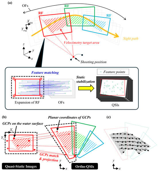
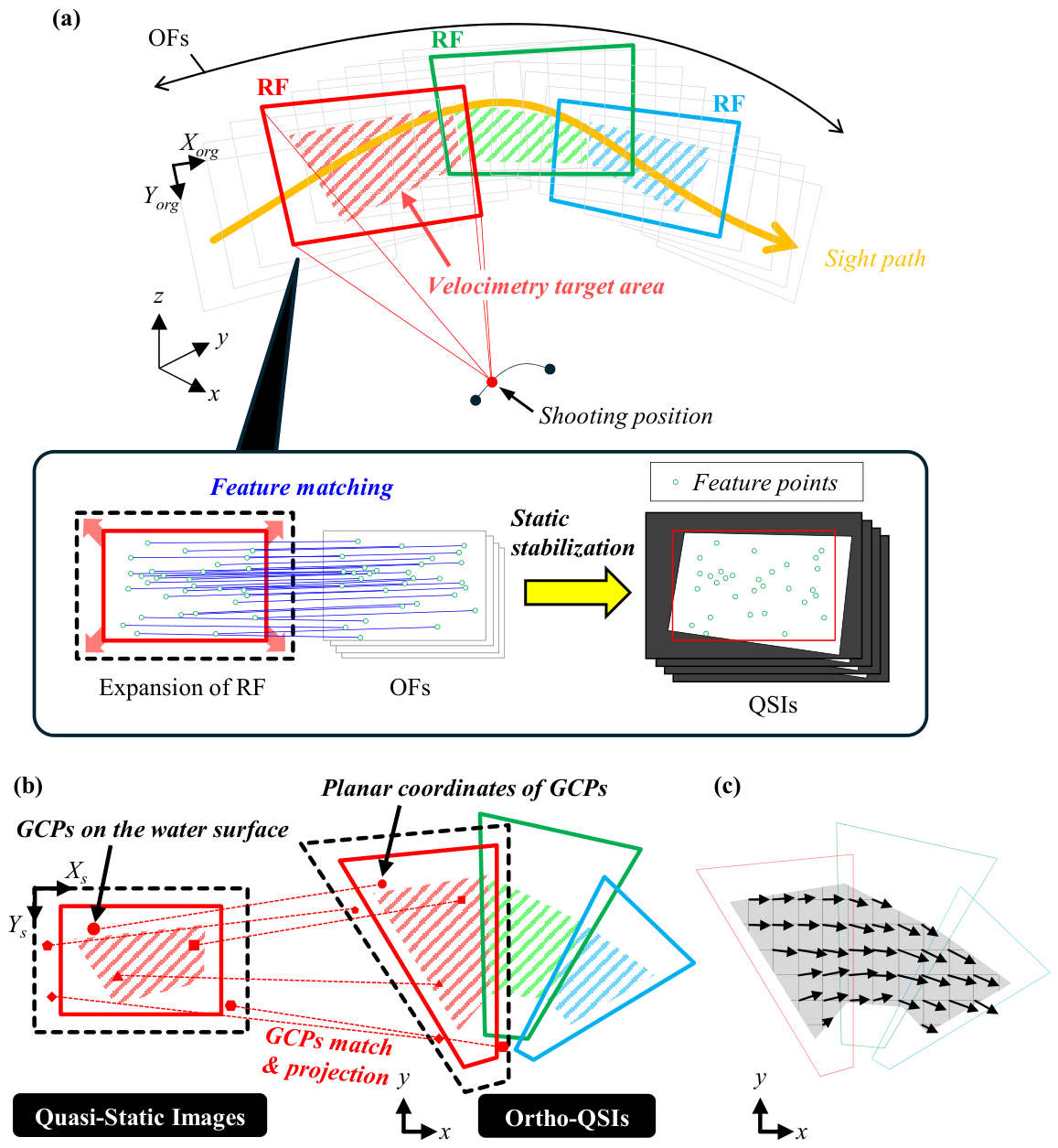
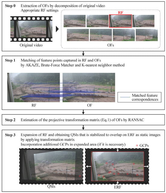
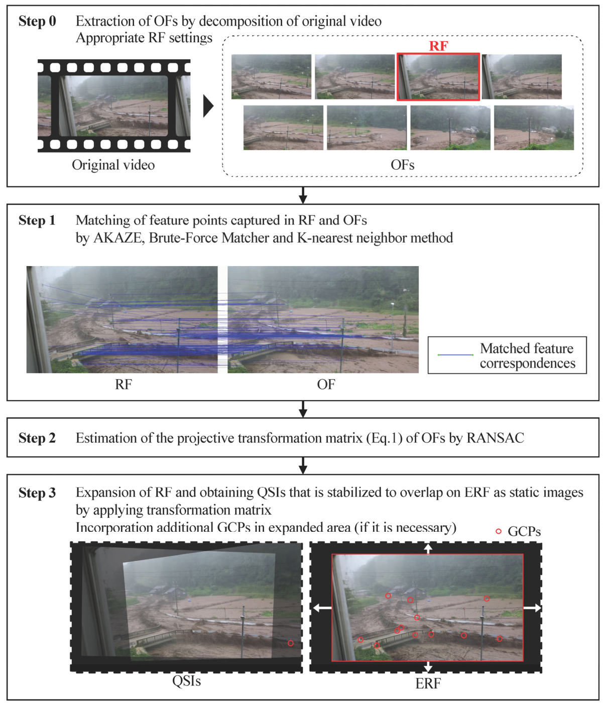
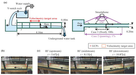
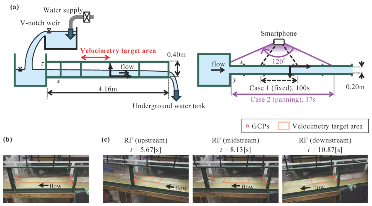
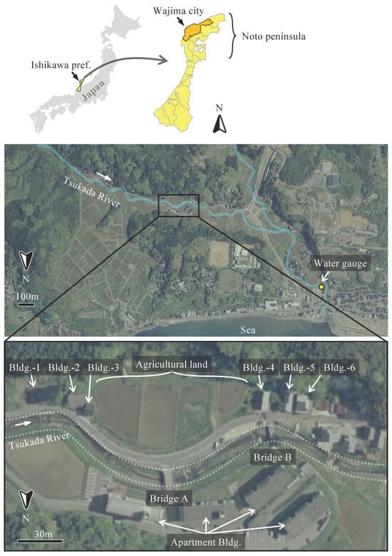
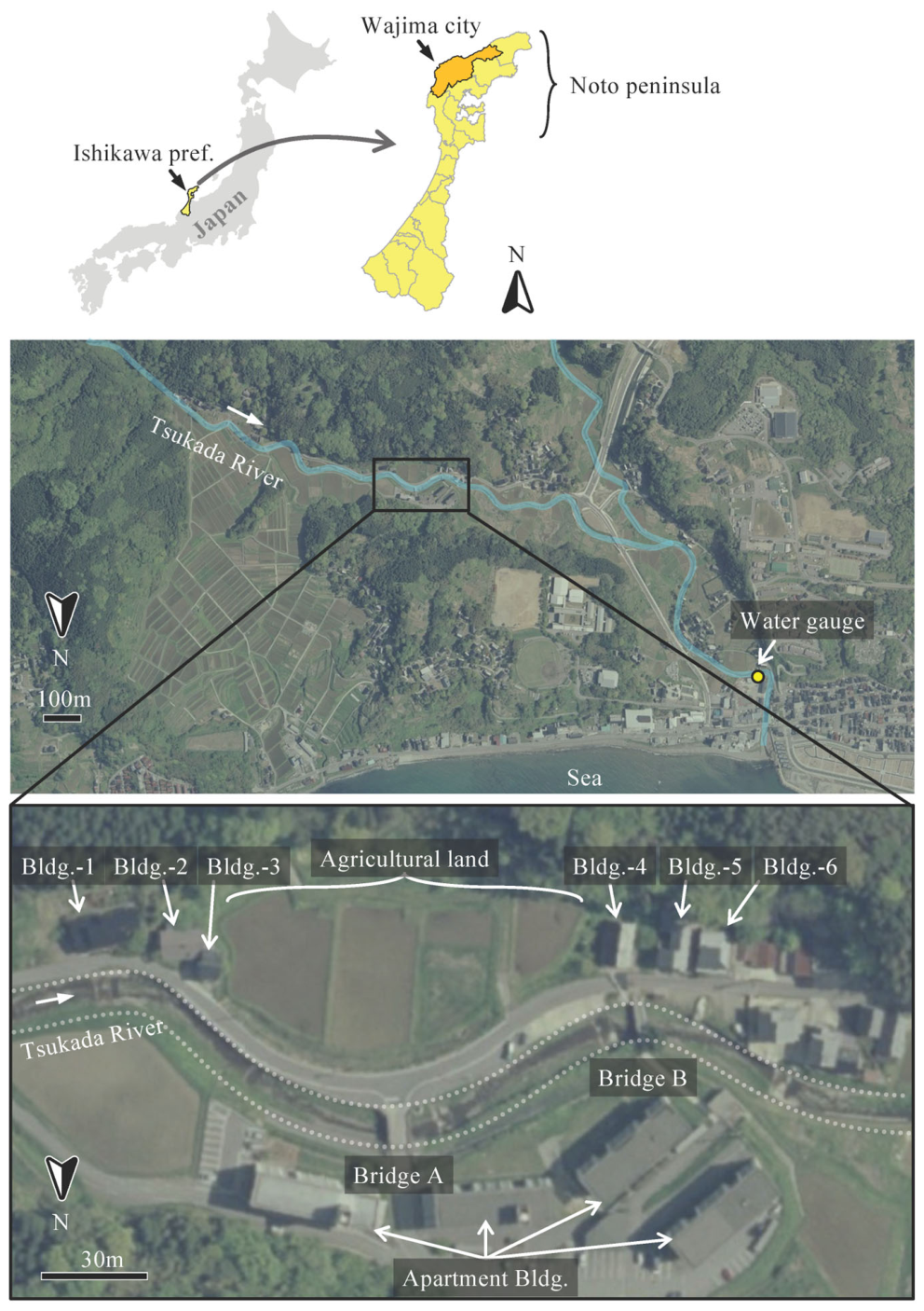
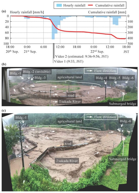
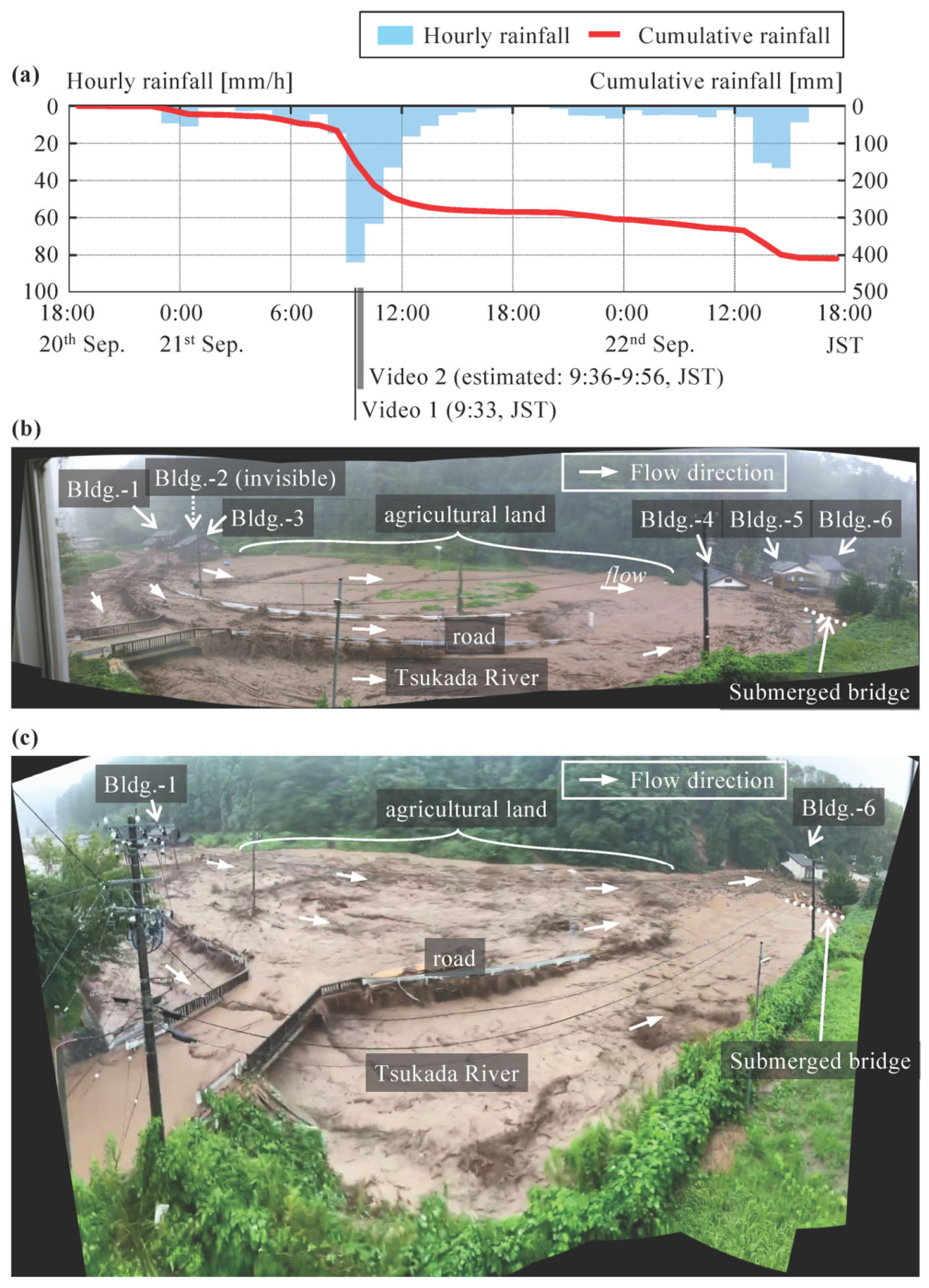
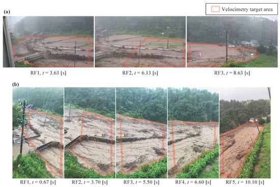
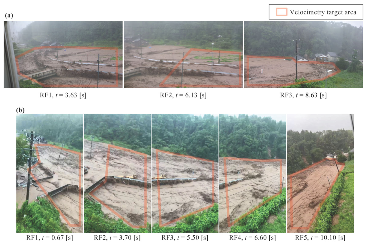
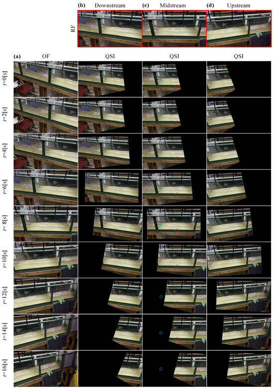
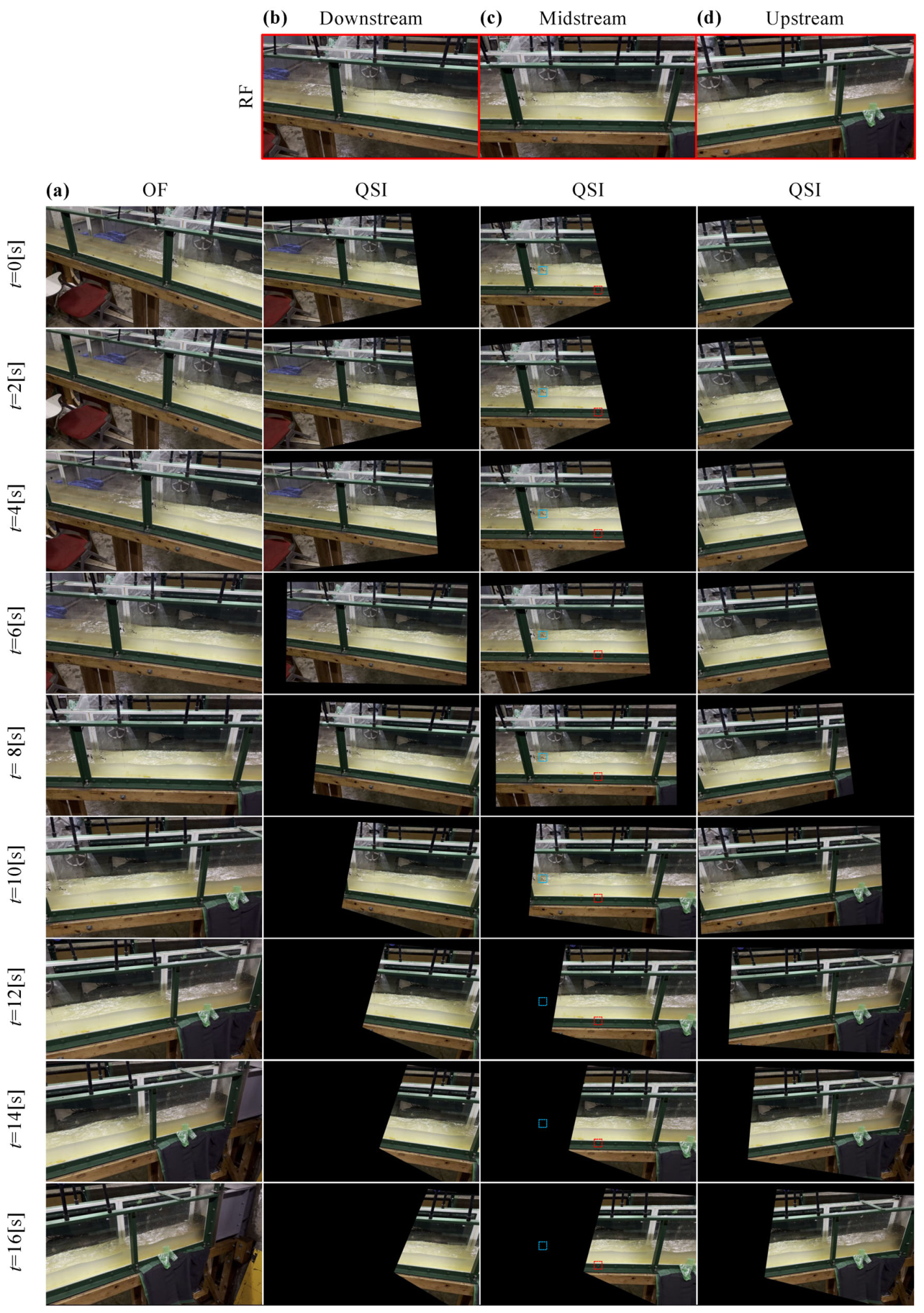
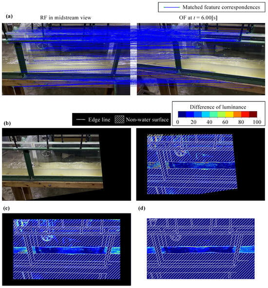
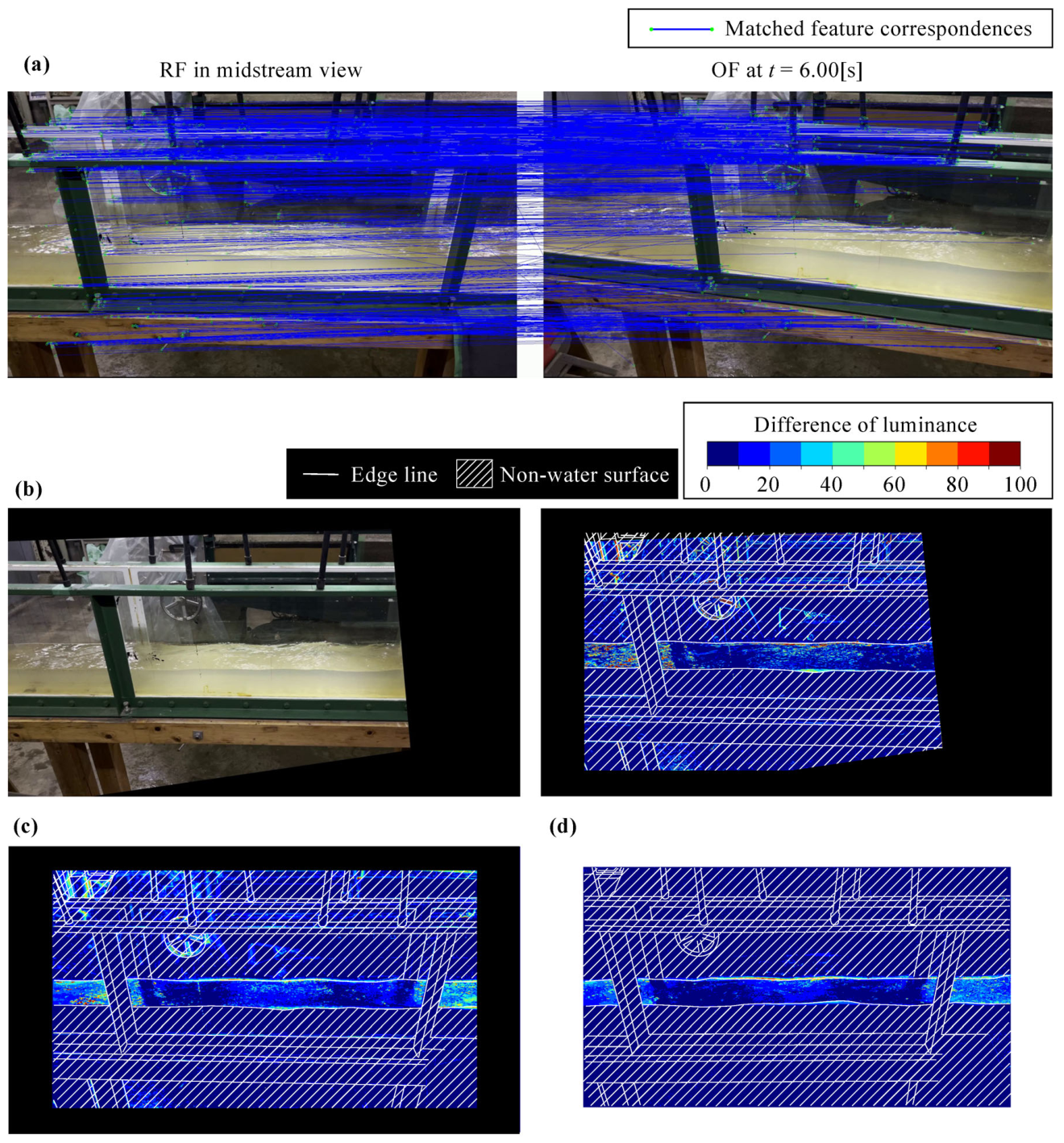
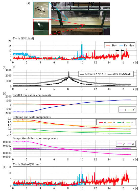
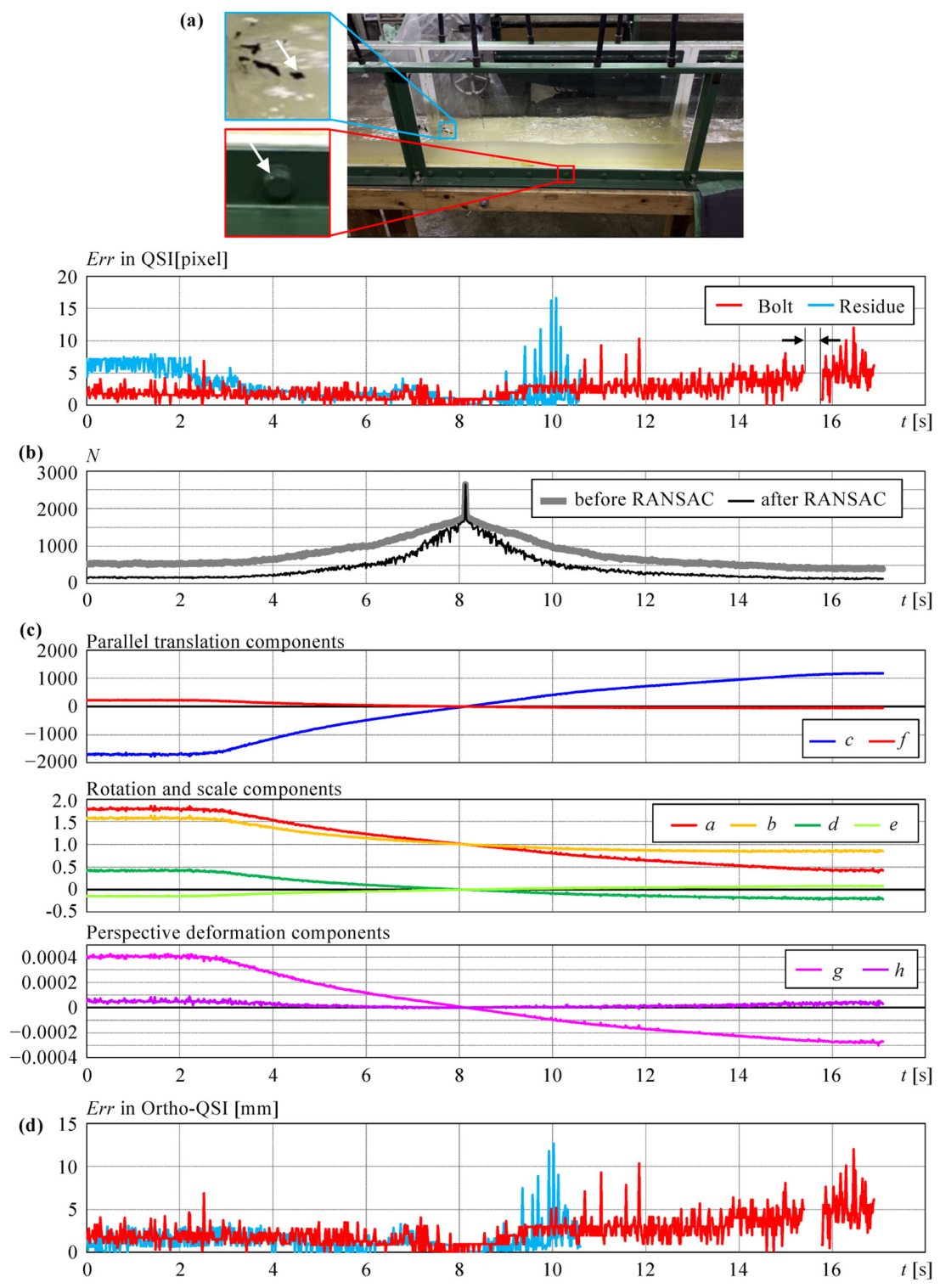
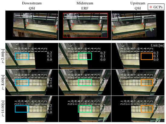
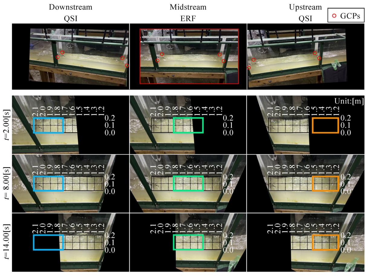
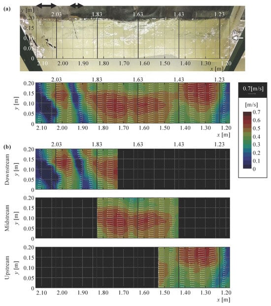
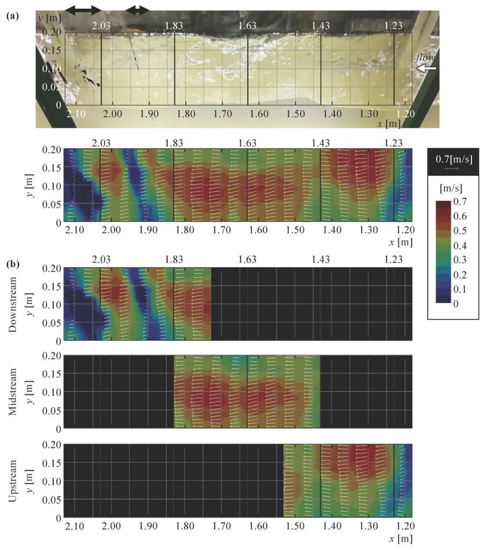
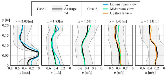
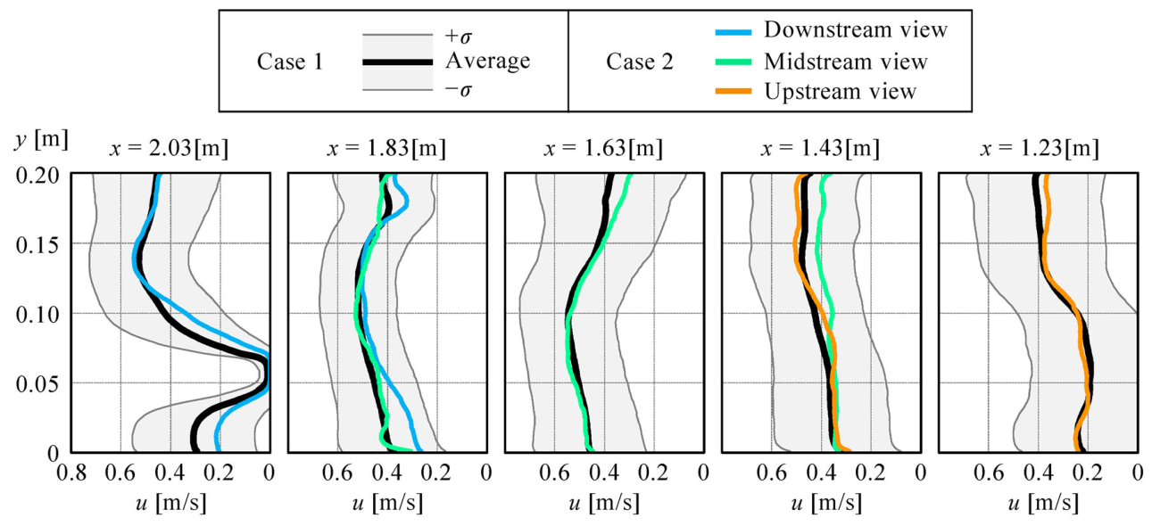
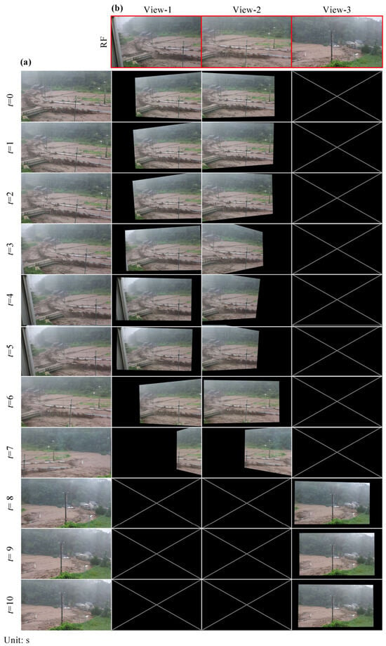
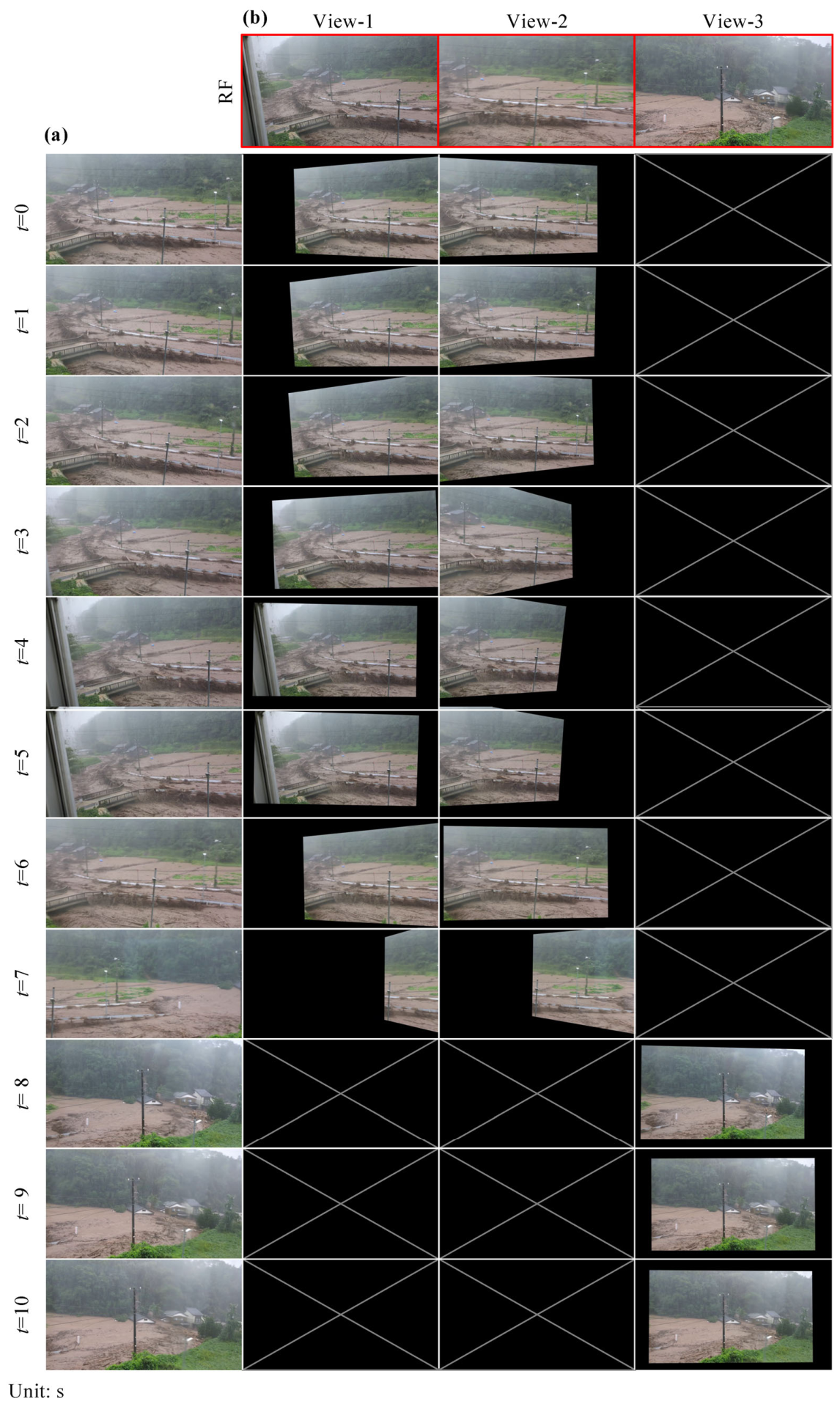
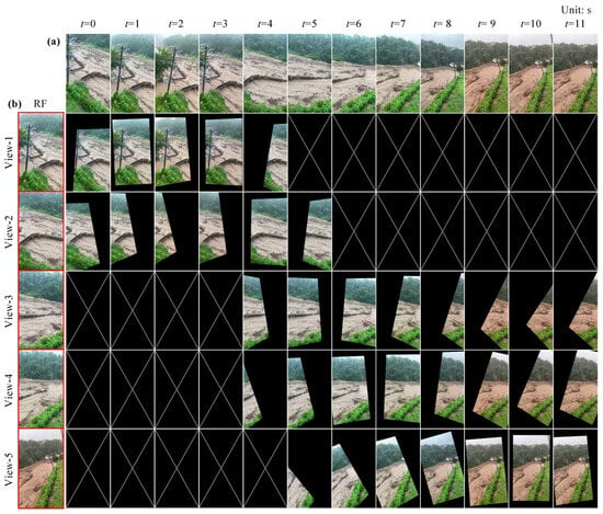
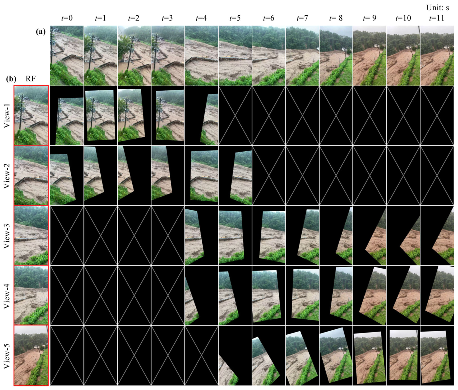
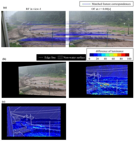
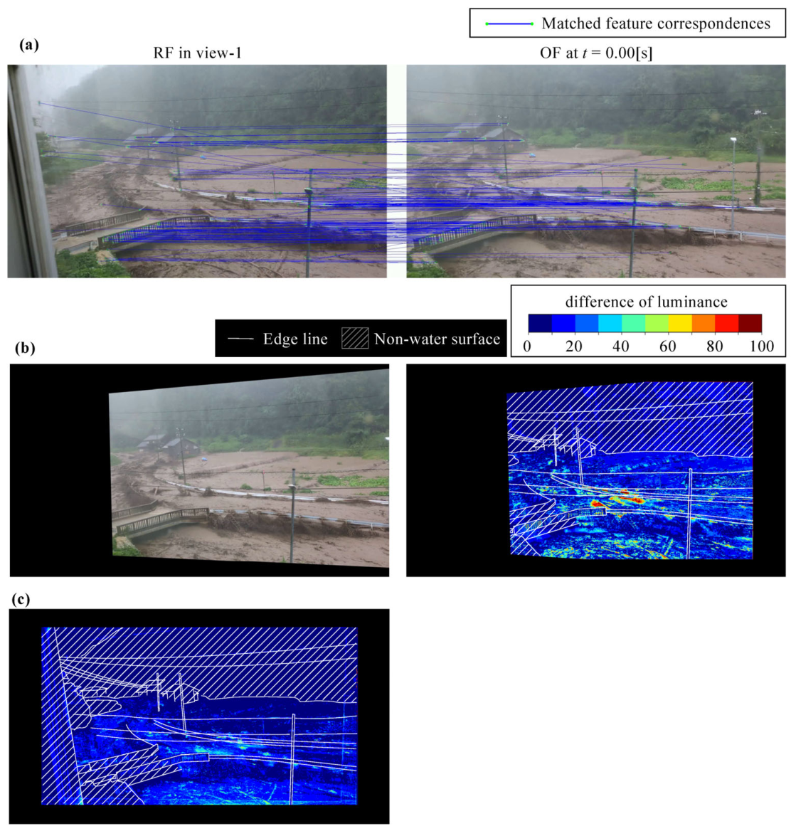
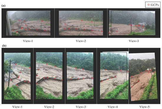
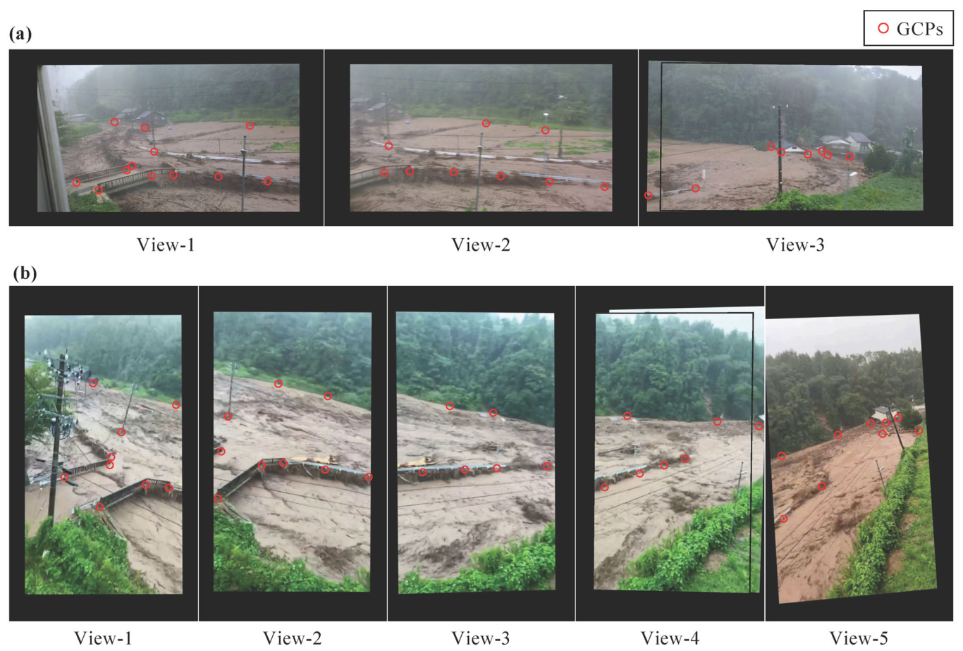
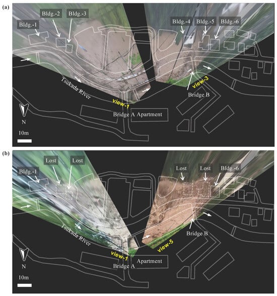
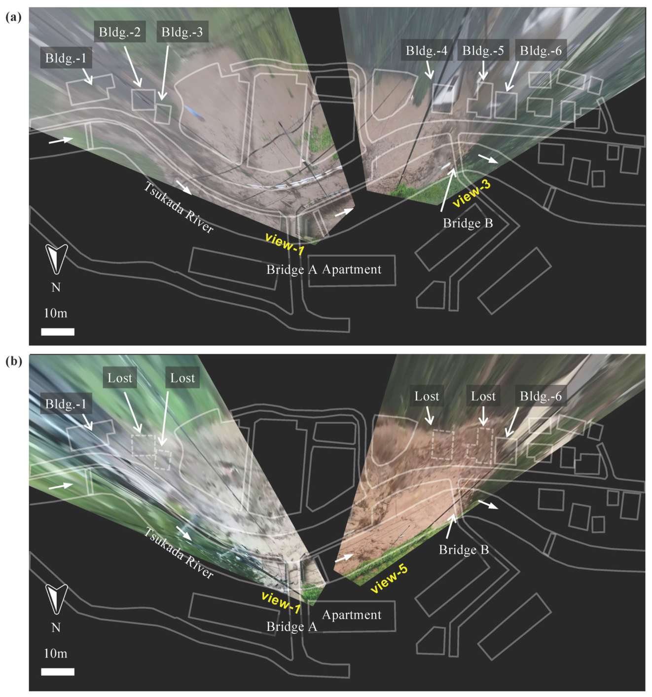
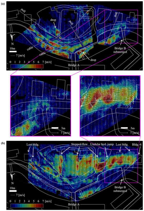
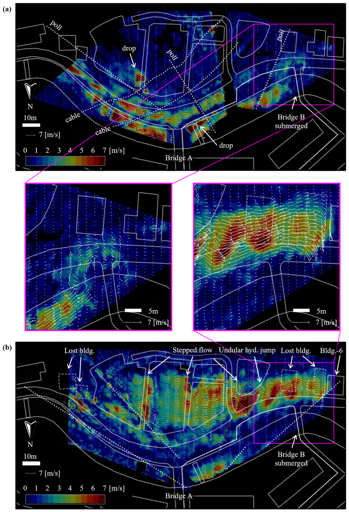

Disclaimer/Publisher’s Note: The statements, opinions and data contained in all publications are solely those of the individual author(s) and contributor(s) and not of MDPI and/or the editor(s). MDPI and/or the editor(s) disclaim responsibility for any injury to people or property resulting from any ideas, methods, instructions or products referred to in the content. |
© 2026 by the authors. Licensee MDPI, Basel, Switzerland. This article is an open access article distributed under the terms and conditions of the Creative Commons Attribution (CC BY) license.