


Abstract
Quantifying glacier contributions to river discharge is challenging because many land surface models (LSMs) lack glacier processes, whereas standalone glacier models are often disconnected from catchment hydrology. Here we develop the Conjunctive Surface–Subsurface Process model version 2-glacier coupled model (CSSPv2-GLC), and evaluate it over the Three-River Headwaters Region (TRHR) at 3 km during 1979–2017. The glacier coupling raises Nash–Sutcliffe Efficiency for monthly streamflow simulation at Tuotuohe station from 0.63 to 0.79 during calibration and from 0.61 to 0.76 during validation. CSSPv2-GLC reduces glacier surface temperature error to 1.85 K, compared with 3.09 K for the CSSPv2. Glacier meltwater contributions to total discharge reached 11.5% in July and 10.8% in August in the Yangtze headwaters. In contrast, the Lancang and Yellow headwaters contributed up to 4.5% and 1.8% in August. Dry-year contributions are 2–3 times higher than wet-year values, indicating a transient drought-buffering effect. These results demonstrate the value of integrating physically explicit glacier processes into land surface modeling frameworks for water resource assessment in glacierized headwater regions, and highlight the necessity of accounting for non-stationary glacier contributions to streamflow.
1. Introduction
Mountain glaciers worldwide are undergoing retreat in a warming climate, altering both the magnitude and seasonal distribution of runoff in glacierized basins. Glaciers act as cryospheric reservoirs that regulate seasonal water availability and buffer interannual hydroclimatic variability [1,2]. Across the Qinghai–Tibet Plateau (QTP), amplified warming has intensified glacier mass loss and reshaped the contribution of meltwater to river discharge [3,4]. As glaciers shift from near-equilibrium conditions toward sustained mass loss, their hydrological role evolves from a quasi-stationary seasonal regulator to a progressively declining and non-stationary water source, challenging the assumption of stationary cryospheric buffering that underpins conventional water resource assessments. Consequently, accurate, process-based quantification of glacier meltwater contributions has become an urgent scientific priority—particularly for high-altitude headwater regions such as the Three-River Headwaters Region (TRHR) on the QTP [5]. Indeed, a comprehensive review by Yao et al. [6] has emphasized that the accelerated transformation of the Asian water tower from solid to liquid conditions is creating a growing imbalance in freshwater availability across downstream basins, underscoring the urgency of developing cryosphere–hydrology coupled models. Recent studies have highlighted the complexity of these hydrological responses. For instance, Wang et al. [7,8] demonstrated significant impacts of cryospheric degradation on terrestrial water storage and discharge regimes across the plateau. Sun et al. [9,10] quantified the shifting partitioning between meltwater and precipitation runoff in headwater basins, emphasizing the non-stationary nature of these contributions. Furthermore, the role of landscape characteristics cannot be overlooked, as Gao et al. [11,12] pointed out that topographic and geomorphological features critically constrain catchment storage and recession behaviors in these alpine environments. Furthermore, Li et al. [13] documented how accelerated multiphase water transformation—including intensified glacier retreat and a declining snowfall-to-precipitation ratio—has fundamentally altered runoff recharge sources in the TRHR, underscoring the need for models to resolve the coupled energy and phase-change processes governing meltwater generation. Achieving such quantification, however, hinges critically on the physical realism of glacier process representation and its hydrological integration within modeling frameworks.
To date, physical process fidelity and hydrological integration have been pursued along largely independent modeling trajectories. Empirical temperature-index (degree-day) methods have been widely embedded within catchment-scale hydrological frameworks (e.g., HBV, VIC, and SWAT) and have demonstrated capability in reproducing observed streamflow in glacierized basins. These methods achieve tight hydrological coupling at low computational cost, yet their reliance on empirical melt factors precludes explicit representation of the radiative and turbulent heat fluxes that often control ablation, limiting parameter transferability across years and climatic regimes [14,15]. Meanwhile, glacier evolution frameworks such as the Open Global Glacier Model (OGGM v1.1) enable efficient large-scale simulations of glacier change but are not designed to close catchment-scale water and energy budgets within a land-surface system [16,17]. More recently, Rounce et al. [16] employed the PyGEM-OGGMv1.1 framework to project global glacier change under warming scenarios, demonstrating that a small increase in temperature matters for glacier mass loss. However, their approach is based on degree-day melt formulations and does not resolve the surface energy budget, limiting its applicability for diagnosing the physical mechanisms of ablation change. Standalone physically based energy-balance models, such as coupled snowpack and ice surface energy and mass balance model in Python (COSIPY v1.3) and distributed energy-balance schemes [18,19,20], achieve high physical fidelity by resolving the full surface energy budget and have advanced mechanistic understanding of glacier mass balance. However, because these models are typically forced offline and lack hydrological closure within broader land surface frameworks, meltwater generation remains disconnected from snowpack evolution, soil hydrology, and runoff routing that collectively determine basin water yield and timing [20,21].
Land surface models (LSMs) provide a promising framework for bridging the gap mentioned above, as they simulate the coupled exchanges of energy, water, and momentum across the entire land surface under consistent atmospheric forcing [22,23,24]. However, glaciers in current LSMs are treated in a highly simplified manner, which are typically represented as permanent snowpack or static ice surfaces with prescribed albedo, lacking a dedicated surface energy balance that resolves radiation, turbulent fluxes, and subsurface heat conduction [23]. The accurate representation of subsurface thermodynamics is particularly challenging. Meng et al. [25] revealed that standard parameterizations of soil thermal conductivity and freeze–thaw processes in current LSMs often lead to significant biases in surface energy partitioning on the Tibetan Plateau. Where glacier melt is parameterized, it generally relies on temperature-index formulations whose empirical coefficients cannot capture the shifting energy partitioning under a warming climate [14,15]. A few recent efforts have begun to embed glacier processes into LSMs, most notably for the Greenland Ice Sheet within CESM/CLM [26] and for Antarctic ice within JULES [24]. Yet, these developments target polar ice sheets at coarse resolution and do not address the distinct requirements of mountain glacier environments, including steep lapse-rate gradients, rapid snow-to-ice albedo transitions, and the dominant role of sublimation in cold continental climates [27,28]. Indeed, a multi-model intercomparison of global glacier projections revealed that structural divergence among model formulations remains the largest source of uncertainty [29,30,31,32], underscoring that physically consistent representation of mountain glacier processes within land surface frameworks is an unresolved issue.
Based on the above literature review, it is found that there is a lack of a coupled land surface–glacier framework that combines physically explicit glacier energy-balance simulation with full hydrological integration at the basin scale, which is critical for reasonably resolving the energy-water coupled processes for the glacier dynamics. To address this gap, we develop CSSPv2-GLC (Conjunctive Surface–Subsurface Process model version 2-glacier), a coupled land surface–glacier model. Building on the CSSPv2 land surface model [33] with a distributed hydrological scheme optimized for complex Tibetan Plateau terrain, we replace the default simplified glacier treatment with a process-based energy balance module that explicitly resolves surface radiation, turbulent heat exchange, multi-layer ice thermodynamics, and dynamic albedo evolution over glacierized grid cells. Through a sub-grid tiling framework, glacier meltwater is seamlessly routed into the catchment hydrological network alongside precipitation-driven runoff, ensuring full mass and energy conservation. Applied over the entire TRHR at 3 km resolution for 1979–2017, we pursue three objectives: (i) to quantify the improvement in monthly streamflow simulation attributable to glacier coupling; (ii) to validate simulated glacier surface temperature and mass balance; and (iii) to diagnose the glacier meltwater contributions across the TRHR.
2. Study Area, Materials and Methods
2.1. Study Area
The TRHR spans approximately 363,000 km2 in the east of the Qinghai–Tibet Plateau, with elevations ranging from 2600 to 6600 m a.s.l. (Figure 1). The region is governed by a continental monsoon climate in which precipitation and peak temperatures coincide during June–September [33]. This warm-wet synchronicity, combined with strong solar radiation exceeding 200 W m−2 in summer, produces complex accumulation–ablation dynamics in which snowfall and melt can occur within the same season and at overlapping elevations.
Figure 1.
Locations of the Three-River Headwaters Region (TRHR) on the Qinghai–Tibet Plateau and evaluation sites. The upper-left inset shows the geographical location of the TRHR within China. The main panel on the right displays the TRHR boundary, major river networks (blue lines), glacier distribution (light blue shading), and elevation (color scale). The Tuotuohe catchment is highlighted in pink. Red stars indicate the four hydrological stations: Tuotuohe (92.45° E, 34.22° N), Zaduo (95.28° E, 32.88° N), Zhimenda (97.20° E, 33.03° N), and Tangnaihai (100.15° E, 35.50° N). The red dot denotes the automatic weather station (AWS). The lower-left inset illustrates the topographic contours and outline of the Xiao Dongkemadi (XDKMD) Glacier, with the arrow indicating its location in the Yangtze River headwaters. The yellow and white shadings show the glacier and non-glacier areas.
Glaciers in the TRHR, with a total area of approximately 2200 km2 as of the CGI-2 baseline, circa 2005 [34], are predominantly of the continental type, characterized by ice temperatures well below the pressure-melting point and substantial mass loss through sublimation—a process that is energetically distinct from surface melt and is often inadequately represented in empirical melt schemes. Glacier coverage exhibits pronounced spatial heterogeneity across the three sub-basins (Figure 1), with 87.7% of the total glacier area located in the Yangtze headwaters, 7.5% in the Lancang headwaters and 4.7% in the Yellow headwaters. [35]. In addition, we also select two sub-areas at finer scale for validation (due to the data availability) as follows:
- (1)
- Catchment scale—the Tuotuohe catchment in the Yangtze River headwaters (Figure 1), with an outlet station at (34.22° N, 92.45° E; 4533 m a.s.l.), has daily discharge records for two non-contiguous periods (1979–1987 and 2007–2016), enabling assessment of model performance under contrasting cryospheric regimes.
- (2)
- Glacier scale—the Xiao Dongkemadi (XDKMD) Glacier (5380–5926 m a.s.l.) in the central Tanggula Mountains, a benchmark monitoring site of the Third Pole Environment program equipped with an on-glacier automatic weather station (AWS, operational since 2005) [36] and continuous stake-based mass balance measurements since 1989 [37], providing the multi-variable observational basis required for process-level validation of surface energy fluxes and mass balance. The observational site is also in the Yangtze River headwaters (Figure 1).
2.2. Data
2.2.1. Meteorological Forcings
The model simulations are driven by China Meteorological Forcing Dataset (CMFD) [38], which provides seven surface meteorological variables (air temperature, pressure, specific humidity, wind speed, downward shortwave and longwave radiation, and precipitation) at 0.1° spatial resolution and 3-hourly temporal resolution for 1979–2018. CMFD merges ground-based station observations with multiple reanalysis products and has been extensively validated over the Tibetan Plateau. The gridded forcing was spatially downscaled to the 3 km model grid using bilinear interpolation, with a fixed environmental lapse rate of −6.5 °C km−1 applied to air temperature and hypsometric adjustments applied to surface pressure [39].
To reduce systematic biases in the forcing data over glacierized surfaces—where station observations are sparse and reanalysis products are known to exhibit substantial errors in temperature and precipitation [40,41]—we applied a variable-specific quantile mapping correction to the air temperature and precipitation fields for the XDKMD Glacier, by using its data from automatic weather stations spanning 2005–2016 [36]. It should be noted that this bias correction was applied exclusively to the XDKMD Glacier grid cells used for point-scale validation. The uncorrected CMFD forcing was used for all regional simulations across the TRHR.
2.2.2. Land Surface and Glacier Data
Static land cover fractions were specified from the ESA CCI 2015 land cover product at 300 m resolution, aggregated to the 3 km model grid [42]. Baseline topography was derived from the 3-arc-second HydroSHEDS digital elevation model (SRTM-based) [43].
Glacier geometry was initialized from the Tibetan Plateau Glacier Inventory circa 1976 (TPG1976) [44], which provides outlines derived from Landsat MSS imagery of the mid-1970s. The initial glacier area in each 3 km grid cell was computed by intersecting the TPG1976 polygons with the model grid. Cells in which the resulting glacier fraction exceeded 5% of the cell area were flagged for explicit treatment by the glacier energy balance module, while cells with smaller glacier fractions were handled by the standard CSSPv2 scheme. Subsequent evolution of glacier area during the transient simulation (1979–2017) was determined prognostically via annual volume–area scaling (Section 2.3.4).
For independent validation of the simulated glacier area trajectory, we employed the long-term glacier boundary dataset of Zhang [45], which provides outlines at approximately decadal intervals (circa 1986, 1995, 2005, 2013, and 2021) derived from multi-source remote sensing. The circa-2005 outlines are consistent with the Second Chinese Glacier Inventory (CGI-2) [34], which reports a total glacier area of approximately 2200 km2 within the TRHR. These observed outlines were used solely for evaluation and were not assimilated into the model.
2.2.3. Validation Data
Multi-source observations were assembled for independent model evaluation. Importantly, all calibration data are clearly distinguished from validation data below to ensure assessment integrity.
- (a)
- Streamflow: Daily discharge records at the Tuotuohe hydrological station were obtained from the Hydrological Yearbook of China for two non-contiguous periods: 1979–1987 and 2007–2016.
- (b)
- Glacier surface mass balance: Annual mass balance at the XDKMD Glacier was compiled from two complementary sources: (i) the in situ stake measurement record for 1989–2016 [33] and (ii) a reconstructed mass balance dataset for seven Tibetan Plateau glaciers covering 1975–2013 [46]. These datasets show high consistency during their overlap period (1989–2013) and were merged to produce a continuous annual series for 1979–2016.
- (c)
- Surface temperature and energy fluxes: Daily clear-sky land surface temperature from MODIS Aqua (MYD11A1, Collection 6; 1 km resolution) [47] for 2000–2017 was used to evaluate simulated glacier surface temperature. In addition, net radiation observations from the XDKMD on-glacier AWS (2008–2010) were used to validate the modeled surface energy partitioning [36].
- (d)
- Albedo (calibration): The snow and ice albedo parameterization (Section 2.3.2) was calibrated against the topography-corrected daily albedo product of Ren et al. [48].
- (e)
- Streamflow used to estimate glacier meltwater contribution in the three head-water sub-basins was derived from hydrological observations at the Zhimenda, Zaduo, and Tangnaihai stations, representing the Yangtze, Lancang, and Yellow River source regions, respectively. These records were obtained from the China Hydrological Year-book and were aggregated to the temporal scale used in the contribution analysis. These stations were used as practical hydrological outlets to represent streamflow from the three headwater sub-basins, although the gauged drainage areas may not be perfectly identical to the glacier inventory-based sub-basin boundaries.
2.3. Model Description
The coupled CSSPv2-GLC model comprises two interacting components (Figure 2): (i) the CSSPv2 LSM, which simulates energy, water and carbon exchanges over non-glacierized terrain, and (ii) a newly developed glacier energy balance module that replaces the simplified glacier treatment in the CSSPv2 with a physically explicit representation of surface energy fluxes, subsurface thermodynamics, and mass changes over glacierized grid cells. At each time step, the two components are driven by identical atmospheric forcings but solved independently on their respective sub-grid tiles. The resulting surface fluxes are area-weighted to yield grid-cell mean values, and glacier meltwater is seamlessly routed into the hydrological network alongside precipitation-driven runoff. The following subsections describe each component.
Figure 2.
Schematic diagram of the coupled CSSPv2-GLC model framework, showing the interaction between the glacier energy-balance module and the CSSPv2 land surface model through a sub-grid tile coupling strategy.
2.3.1. CSSPv2 Land Surface Model
The non-glacierized fraction of each grid cell is simulated by the Conjunctive Surface–Subsurface Process model version 2 (CSSPv2) [33,49]. CSSPv2 explicitly resolves lateral surface and subsurface flows, which is a critical capability for representing the topography-driven drainage patterns over mountainous areas. CSSPv2 also incorporates a storage-based runoff generation scheme, together with organic-matter-dependent soil thermal and hydraulic parameterizations tailored to alpine environments. Previous high-resolution (3 km) simulations over the TRHR demonstrated that CSSPv2 significantly outperforms global reanalysis products in reproducing soil moisture, evapotranspiration, and streamflow, and successfully captures elevation-dependent warming trends [33]. In the default CSSPv2 configuration, glacierized grid cells are treated as permanent snowpack with static albedo and single-layer snow thermodynamics, which—as demonstrated in the Introduction—is physically inadequate for resolving ablation-season energy partitioning.
2.3.2. Glacier Energy Balance Module
To enable explicit simulation of glacier processes, we developed a glacier energy balance module that is coupled with CSSPv2. The module calculates the surface energy balance over glacierized grid cells and simulates the resulting mass changes.
The glacier surface energy balance is expressed as [14]:
where is the energy available for surface processes (W ), is incoming shortwave radiation (W ), is surface albedo, is surface emissivity, is incoming longwave radiation (W ), is the Stefan–Boltzmann constant, is the surface temperature (K), is the sensible heat flux (W ), is the latent heat flux (W ), and is the heat flux from precipitation (W ). Three key parameterizations govern the energy partitioning and are summarized below.
- (1)
- Surface albedo: The albedo scheme distinguishes snow cover from bare ice surfaces and accounts for snow aging, solar zenith angle, and snow depth. For snow-covered conditions, albedo decays exponentially with cumulative exposure time in both the visible and near-infrared bands. The transition from snow to bare-ice albedo is governed by an exponential snow depth decay function [18]:
The two coefficients were calibrated by grid search against the albedo product of Ren et al. [48], with search ranges setting to physically plausible bounds: a ∈ [0.003, 0.020] K−1 and b ∈ [0.45, 0.70]. The calibrated values are a = 0.0084 K−1 and b = 0.6487, consistent with the physically expected sensitivity of bare-ice reflectance to surface moisture conditions at continental high-altitude glaciers on the Qinghai–Tibet Plateau. This captures the observed dependence of bare-ice reflectance on surface moisture conditions: wetter (warmer) surfaces exhibit lower albedo due to meltwater film formation and enhanced particulate concentration. The albedo scheme was calibrated against the topography-corrected daily albedo product of Ren et al. [48] (Section 2.2.3d)
- (2)
- Turbulent Heat Fluxes: Sensible and latent heat fluxes are computed using Monin-Obukhov similarity theory with an iterative stability correction scheme [50]
- (3)
- Refreezing: The refreezing parameterization employs a dual-constraint scheme that explicitly limits refreezing by both the available cold content of each snow layer and the pore-space liquid water retention capacity at the snow–ice interface. This physically based treatment avoids the systematic overestimation of refreezing that can arise from simpler temperature-threshold approaches [54].
Conversely, if the temperature falls below freezing temperature and liquid water is present, refreezing occurs. The refreezing parameterization explicitly accounts for two physical constraints. First, the maximum refreezing rate in each snow layer is limited by the available cold content:
where the first term represents the cold-content-limited refreezing capacity and the second term ensures that refreezing cannot exceed the available liquid water. Second, at the snow–ice interface, refreezing is additionally constrained by the pore-space water retention capacity:
where is the porosity, is the liquid water density (kg m−3), and is the capillary retention coefficient. The released latent heat from refreezing raises the layer temperature accordingly. This dual-constraint refreezing scheme provides a more physically consistent treatment than simple temperature-based parameterizations commonly used in glacier models.
2.3.3. Glacier–LSM Coupling
The glacier module is integrated with CSSPv2 using a sub-grid tile approach. Each model grid cell is partitioned into a glacierized fraction () and a non-glacierized fraction () based on the glacier mask derived from TPG1976. Both fractions are driven by the same atmospheric forcing at each time step but solved independently: the glacierized fraction uses the glacier energy balance module described above, while the non-glacierized fraction uses the standard CSSPv2 land surface scheme. The grid-cell mean surface fluxes are computed as area-weighted averages:
where and denote fluxes from the glacier and non-glacier tiles, respectively. This applies to all output fluxes including sensible heat, latent heat, outgoing longwave radiation, and surface runoff.
Meltwater generated by the glacier module, including surface melt, internal melt, and rainfall on ice, is collected as glacier runoff:
where is the internal melt from subsurface phase change (kg m−2). This glacier runoff is added to the surface runoff of the corresponding grid cell and subsequently routed through the river network along with runoff from non-glacierized areas, using the same kinematic wave routing scheme [55] employed by CSSPv2. At each 3-hourly time step, the glacier module computes glacier runoff as the sum of surface melt, internal melt, and rainfall on ice, minus sublimation losses. is area-weighted by the glacier fraction and combined with non-glacierized runoff to yield the total surface runoff of the grid cell. The combined runoff is then routed downstream on the HydroSHEDS river network using the same kinematic-wave scheme as CSSPv2. This treatment ensures mass-conservative integration of glacier meltwater into the basin hydrological system.
2.3.4. Glacier Geometry Update
To represent the transient evolution of glacier extent over the simulation period, the coupled model employs an annual geometry update scheme based on volume–area (V–A) scaling. This approach translates the cumulative surface mass balance simulated by the glacier energy balance module (Section 2.3.2) into changes in glacier volume and, subsequently, glacier area within each grid cell. The V–A scaling method provides a computationally efficient yet physically grounded alternative to explicit ice flow dynamics.
Following Bahr et al. [56], glacier volume (km3) is related to glacier area (km2) through:
where and , which were adopted from the empirical calibration of Radić and Hock [57] for High Mountain Asia glaciers and were consistent with the theoretical derivation of Bahr et al. [56]. For reference, the published range for mountain glaciers is γ ∈ [1.25, 1.50] and c ∈ [0.02, 0.08] depending on glacier type and region [58]. The calibrated values fall within this range and correspond to the High Mountain Asia subset of the Radić and Hock [57] global calibration. While this approach provides a computationally efficient first-order approximation on decadal timescales, it assumes quasi-equilibrium glacier geometry and cannot resolve the mass–elevation feedback (whereby surface lowering exposes ice to warmer temperatures at lower elevations) or ice-dynamic processes such as flow acceleration. These limitations are discussed further in Section 4.4.
2.3.5. Standalone Benchmark Model COSIPY
To isolate the value of embedding glacier physics within a land surface framework, we employ the COSIPY [18] as a standalone benchmark. COSIPY is an open-source, physically based model that solves the surface energy balance over a one-dimensional snow–ice column and has been applied to mountain glaciers across a range of climatic settings
COSIPY and the CSSPv2-GLC glacier module share the same fundamental physical framework. They both solve the full surface energy budget, simulate multi-layer snow–ice thermodynamics, and parameterize albedo evolution with snow aging. However, CSSPv2-GLC introduces several process-level refinements relative to COSIPY. In particular, CSSPv2-GLC’s surface albedo scheme not only represents snow aging and snow-depth-controlled snow-to-ice transition, but also parameterizes bare-ice albedo as a function of surface dewpoint temperature, thereby allowing the radiative effect of surface moisture conditions to be represented explicitly. In addition, CSSPv2-GLC adopts a dual-constraint refreezing scheme in which refreezing is limited jointly by the available cold content of each snow layer and the pore-space liquid-water retention capacity at the snow–ice interface, whereas COSIPY uses its own snow-aging albedo formulation and bucket-type meltwater percolation/refreezing treatment. These differences reflect the structural uncertainty inherent in glacier energy balance modeling and are representative of the diversity encountered in the broader glacier modeling community [31,32]. In this study, COSIPY was driven by the same bias-corrected CMFD meteorological forcings applied to the glacier tiles in CSSPv2-GLC (Section 2.2.1), ensuring that differences in model performance stem from the model formulation and coupling architecture rather than from differences in atmospheric input.
2.4. Experimental Design
2.4.1. Numerical Experiments
For clarity, the overall workflow of the numerical experiments and evaluation strategy is summarized in Figure 3
Figure 3.
Experimental workflow of the study.
Three numerical experiments were conducted to progressively isolate the contributions of explicit glacier energy balance physics and the LSM coupling framework (Table 1). All experiments were driven by the same bias-corrected atmospheric forcings (Section 2.2.1) during 1979–2017. The experiments differ exclusively in their treatment of glacierized grid cells.
Table 1.
Summary of numerical experiments.
2.4.2. Initialization and Spin-Up
All simulations were initialized from climatological soil temperature and moisture profiles. To bring the deep soil and glacier ice columns into thermodynamic quasi-equilibrium, a recursive spin-up procedure was applied, where the 1979–2017 atmospheric forcing sequence was cycled through the model three times consecutively. Convergence was assessed by checking the annual mean temperature at all resolved depths in the glacier ice column (2 m, 10 m, and 20 m) across successive spin-up cycles. The absolute inter-cycle drift, computed from the 5-year tail-mean of each cycle, declined to 0.040 K at 2 m, 0.057 K at 10 m, and 0.058 K at 20 m by the end of simulation cycle 3, whereas the simulations cycle 2–cycle 1 drift at 20 m depth was still 0.571 K. These results indicate that a single simulation cycle would be insufficient and that three full cycles of the 1979–2017 forcing sequence (117 model years in total) were necessary to achieve thermodynamic quasi-equilibrium of the glacier ice thermal state.
A split-sample calibration–validation framework was adopted to evaluate model performance and ensure temporal transferability. The non-contiguous calibration period (1979–1987) and validation period (2007–2016) were determined by the availability of observed discharge data at Tuotuohe station, as no reliable continuous observations were available for the intervening years. The model was run continuously over 1979–2017 with one fixed parameter set, without reinitialization or recalibration during the gap years. Although model performance during the intervening period cannot be directly verified, the ability of one parameter set to reproduce streamflow reasonably well in both the early and late observed periods, separated by nearly two decades, provides evidence for the model temporal transferability under non-stationary hydroclimatic and cryospheric conditions.
The hydrological parameters controlling runoff generation and river routing were adopted from Yuan et al. [33] without modification. The parameters were calibrated over the TRHR against observed streamflow at multiple stations. Other land surface parameters in CSSPv2 (soil hydraulic and thermal properties, vegetation parameters) were adopted directly from the configuration of Yuan et al. [33] without further calibration against the discharge data used for validation in this study. This ensures strict independence between the model parameter set and the validation target. The only calibrated parameters in the coupled system are the glacier surface albedo coefficients, which were constrained against the independent albedo product of Ren et al. [48] prior to the validation experiments (Section 2.2.3).
2.4.3. Evaluation Metrics
Model evaluation was structured around the nested validation network described in Section 2.1. Table 2 summarizes the validation variables, observational data sources, spatial scales, and analysis periods:
Table 2.
Validation variables, data sources, and analysis periods.
Model performance was quantified using four metrics [59,60]: Nash–Sutcliffe Efficiency (NSE), Bias, Root Mean Square Error (RMSE), and Pearson Correlation Coefficient (CC).
3. Results
A consolidated summary of model performance metrics across all validated variables is provided in Table 3.
Table 3.
Model performance summary for CSSPv2, CSSPv2-GLC, and COSIPY.
3.1. Validation of Land Surface Temperature Simulation at Xiao Dongkemadi Glacier
Accurate simulation of surface temperature (Ts) is a fundamental prerequisite for resolving the glacier energy budget, as it governs outgoing longwave radiation, turbulent heat fluxes, and the onset of ablation. We evaluated the daily climatological Ts (2000–2017) against MODIS Aqua (MYD11A1) clear-sky retrievals (Figure 4).
Figure 4.
Validation of simulated glacier surface temperature and net radiation at Xiao Dongkemadi (XDKMD) Glacier. (a) Seasonal cycle of glacier surface temperature, comparing MODIS observations (OBS; black solid line) with simulations from CSSPv2-GLC (red solid line), COSIPY (blue dashed line), and CSSPv2 (green dash-dotted line). (b) Seasonal cycle of net radiation, comparing in situ observations from the XDKMD automatic weather station (OBS; black solid line) with simulations from CSSPv2-GLC (red solid line), COSIPY (blue dashed line), and CSSPv2 (green dash-dotted line).
All three simulations reproduce the seasonal cycle, transitioning from winter minima (~248 K) to the physical melting-point constraint (273.15 K) in summer (Figure 4a). However, the models differ markedly in quantitative fidelity. CSSPv2-GLC shows closer agreement with MODIS (RMSE = 1.85 K, Bias = −0.15 K, CC = 0.97), whereas COSIPY exhibits a substantially larger error (RMSE = 3.09 K, Bias = +0.82 K, CC = 0.92). The discrepancy is most pronounced during the cold season (October–March), when COSIPY displays high-frequency fluctuations and intermittent warm biases of 3–5 K (Figure 4a). These oscillations are a direct consequence of the shallow computational domain in the standalone model: without the deep subsurface thermal solver provided by the LSM host, the thin snow–ice column responds too rapidly to transient atmospheric perturbations, lacking the thermal inertia needed to buffer short-term forcing variability. In contrast, CSSPv2-GLC benefits from the multi-layer soil–ice thermal continuum of CSSPv2, which stabilizes through realistic subsurface heat storage.
The comparison with the uncoupled baseline (CSSPv2) isolates the value of the explicit glacier module (Figure 4a). The baseline systematically overestimates ablation-season by 2–5 K (Bias = +1.36 K), a bias that arises from its “snowpack” representation: once the seasonal snow depletes, the default scheme exposes a low-albedo soil surface that lacks the latent heat sink associated with ice melt. The resulting energy surplus is erroneously directed toward sensible heating rather than phase change, driving above the physical limit of a melting glacier surface. By explicitly partitioning surplus energy into the latent heat of fusion, CSSPv2-GLC substantially reduces this warm bias and more closely reproduces the observed temperature.
To diagnose the radiative mechanisms underlying these temperature improvements, we validated the simulated net radiation () against in situ observations from the XDKMD on-glacier AWS (2008–2010; Figure 4b). CSSPv2-GLC reproduces the observed seasonal cycle with high skill (CC = 0.88, RMSE = 21.27 W m−2), more closely capturing the transition from negative winter fluxes to peak summer values of approximately 50 W m−2. COSIPY overestimates the seasonal amplitude, producing excessive radiative cooling in winter (~−40 W m−2) and excessive gains in summer (~+50 W m−2), suggesting that its albedo scheme undergoes overly abrupt transitions between snow and ice optical properties. The uncoupled CSSPv2 baseline exhibits a large positive bias (+51.73 W m−2) throughout the year, driven by the albedo contrast between the dark soil surface exposed in the control run (albedo ~0.2–0.3) and the brighter bare ice (albedo ~0.4–0.6) appropriately represented in the coupled model. By resolving the snow-to-ice albedo transition rather than a snow-to-soil transition, CSSPv2-GLC reduces the RMSE by 63% relative to the baseline (from 58.01 to 21.27 W m−2).
3.2. Validation of Glacier Surface Mass Balance Simulation at Xiao Dongkemadi Glacier
We validated the simulated annual SMB against the long-term in situ record (1979–2016) at XDKMD Glacier (Figure 5), a critical reference for the central Tibetan Plateau. CSSPv2-GLC exhibits high fidelity in reproducing both the interannual variability and the trend of glacier mass. CSSPv2-GLC achieves a robust agreement with observations (CC = 0.76, RMSE = 345 mm w.e. yr−1), substantially outperforming the standalone COSIPY model (CC = 0.36, RMSE = 428 mm w.e. yr−1). This suggests that without the buffering effects of a coupled land surface (e.g., sublimation feedbacks and realistic snowpack persistence), the standalone energy balance solution is overly sensitive to instantaneous atmospheric forcing. In addition, the observations reveal a regime shift from near-equilibrium in the 1980s (mean SMB: ~−180 mm w.e. yr−1) to accelerated mass loss in the post-2000s (mean: ~−420 mm w.e. yr−1). CSSPv2-GLC reproduces the observed negative tendency more realistically, whereas COSIPY does not capture this shift and therefore tends to underestimate cumulative water loss in recent decades.
Figure 5.
Validation of simulated annual surface mass balance (SMB; mm w.e. yr−1) at XDKMD Glacier (1979–2016). The black line represents in situ observations (OBS); the red line represents the CSSPv2-GLC simulation; and the blue line represents the COSIPY model output. The dashed horizontal line indicates the zero-balance threshold.
To assess trend significance, we applied the Mann–Kendall test to the observed and simulated annual SMB series. For the observed series (1979–2016), the test yields τ = −0.097 (z = −0.84, p = 0.40), indicating no statistically significant monotonic trend, consistent with the high interannual variability (σ = 343 mm w.e. yr−1) that masks the underlying signal. For CSSPv2-GLC, τ = −0.175 (z = −1.53, p = 0.125), consistent with the observed trend direction. In contrast, COSIPY yields a positive trend with τ = +0.169 (p = 0.137), indicating an opposite tendency that is physically inconsistent with the warming-driven mass loss expected for the study period. A Pettitt change-point test applied to the CSSPv2-GLC series identifies a regime shift around year 1997 (K = 181, p = 0.061), separating a near-equilibrium phase (1979–1989 mean: −182 mm w.e. yr−1) from a stronger mass-loss phase (2000–2016 mean: −369 mm w.e. yr−1).
To assess the model’s ability to represent transient glacier retreat, we derived the annual glacier area change rate from the simulated cumulative mass balance using volume–area scaling and compared the results against the decadal glacier outlines of Zhang [45] (Figure 6). CSSPv2-GLC achieves substantially lower errors in reproducing the observed rate of glacier area change across all three sub-basins, with RMSE values of 1.00, 0.88, and 0.88 km2 yr−1 for the Yangtze, Lancang, and Yellow River source regions, respectively, which are approximately half the corresponding COSIPY errors of 1.96, 1.96, and 1.72 km2 yr−1. The larger errors in the COSIPY model arise from the cumulative propagation of the mass balance biases identified in Section 3.2. Without the stabilizing effect of land surface feedbacks, COSIPY tends to overestimate mass turnover, leading to exaggerated interannual fluctuations in geometric retreat rate. The consistently lower RMSE of CSSPv2-GLC indicates that the coupled framework successfully translates improved energy–mass partitioning into reliable geometric evolution, which is critical for long-term projections because the rate at which glacier area shrinks directly controls the surface available for future melt generation.
Figure 6.
Comparison of model performance in simulating the rate of glacier area change across the TRHR. The bar chart displays the Root Mean Square Error (RMSE) of the simulated annual glacier area change rate (km2 yr−1) for the CSSPv2-GLC (red) and COSIPY (blue-green) models across the Yangtze River, Lancang River, and Yellow River source regions.
3.3. Validation of Streamflow Simulation over the Tuotuohe Catchment
We evaluated the model’s ability to reproduce monthly discharge at the Tuotuohe station across the calibration period (1979–1987) and the independent validation period (2007–2016) (Figure 7). Because CSSPv2 and CSSPv2-GLC share identical hydrological parameters calibrated during Period I, any performance difference between the two configurations is attributable exclusively to the glacier coupling. During the calibration period (Period I), CSSPv2-GLC achieves a NSE of 0.79, compared with 0.63 for the uncoupled CSSPv2 baseline. This improvement is noteworthy because both models were calibrated with the same parameter set, and the additional skill of CSSPv2-GLC arises entirely from the explicit simulation of glacier meltwater, which supplements precipitation-driven runoff during the ablation season.
Figure 7.
Validation of simulated monthly streamflow at Tuotuohe station. (a) Calibration period (1979–1987). (b) Validation period (2007–2016). The results are from observation (black lines), CSSPv2-GLC simulation (red lines) and CSSPv2 simulation (blue lines).
Figure 7 shows that CSSPv2 systematically underestimates summer peak flows, particularly in July and August. This is because the default CSSPv2 treats glacierized areas as seasonal snowpack, where once the winter snow is depleted (typically by June), the model produces no further meltwater from the ice reservoir, cutting off the glacier contribution during the ablation season. In contrast, CSSPv2-GLC activates the glacier energy balance module and sustains meltwater generation through the summer by explicitly simulating energy-driven ablation of the ice column. This improvement reduces the underestimation of July–August discharge, especially for the peaks in 1981, 1982, 2009, and 2010.
To assess whether the NSE improvements are statistically robust, we applied a moving block bootstrap test (10,000 resamples, block length = 12 months) to the monthly streamflow residuals. Because the coupling of an explicit glacier module is physically expected to improve rather than degrade streamflow simulation, a one-sided test at the 90% confidence level was adopted. In the calibration period (1979–1987), the improvement is positive (ΔNSE = 0.136) with a one-sided p-value of 0.050, indicating a statistically significant improvement at the 90% confidence level. In the validation period (2007–2016), the improvement is larger (ΔNSE = 0.216) with a one-sided p-value of 0.001 and a two-sided 90% confidence interval of [0.071, 0.308] that does not include zero, further confirming a statistically significant improvement.
3.4. Spatiotemporal Characteristics of Glacier Meltwater Contributions
Having validated the CSSPv2-GLC model’s ability to simulate glacier surface temperature, mass balance, and streamflow, we now apply the model to diagnose the spatiotemporal characteristics of glacier meltwater contributions to river discharge across the TRHR. Glacier meltwater is computed as the sum of surface melt, internal melt, and rainfall on ice surfaces, minus sublimation losses, and is routed into the hydrological system through the tile-based coupling framework.
3.4.1. Long-Term Evolution of Glacier Geometry and Meltwater Production
Figure 8 shows that during Phase I (1981–circa 1997), glacier area declined gradually from approximately 2140 to 2100 km2, and the polynomial meltwater trend declined in parallel from approximately 22 × 106 m3 yr−1 to a minimum of approximately 15 × 106 m3 yr−1. During Phase II (circa 1997–2017), glacier area continued its monotonic decline (from ~2100 to ~2010 km2), yet the meltwater trend reversed direction, rising from its minimum back to approximately 22 × 106 m3 yr−1 by 2017. This divergence—rising meltwater yield from a diminishing ice reservoir—is characteristic of the ascending limb of the “peak water” trajectory described by Huss and Hock [2]. The year-to-year variability in meltwater volume is substantial throughout the record (ranging from approximately 5 to 33 × 106 m3 yr−1), reflecting the strong interannual modulation of melt rates by summer temperature and radiation anomalies.
Figure 8.
Co-evolution of simulated glacier area (blue line, left axis), annual meltwater volume (orange bars, right axis) and its polynomial meltwater trend (red dashed line) in the TRHR from 1979 to 2017.
3.4.2. Seasonal Dynamics of Glacier Meltwater Contribution
The glacier meltwater contribution to total streamflow exhibits a strongly seasonal pattern governed by the annual cycle of surface energy availability, with marked differences in magnitude and timing among the three source sub-basins (Figure 9). Across all three sub-basins, melt contributions are negligible during the cold season (November–March, <1% of total discharge). Contributions begin to increase in April–May as incoming solar radiation intensifies and surface temperatures approach the melting point, and peak in July–August during maximum ablation-season energy input when the snowline has retreated to expose bare glacier ice.
Figure 9.
Multi-year mean monthly glacier meltwater contribution to total streamflow (%) for the Yangtze River source (blue), Lancang River source (orange), and Yellow River source (green) sub-basins. The streamflow data used for calculating glacier contributions were compiled from the Zhimenda, Zaduo and Tangnaihai for Yangtze, Lancang and Yellow river sources (Figure 1). Peak contributions annotated in each sub-basin.
The Yangtze River source, which hosts the most extensive and highest-elevation glaciers in the Tanggula Mountains, exhibits the most pronounced and sustained seasonal melt. Contributions rise from approximately 2% in April to a peak of 11.5% in July, remain elevated at approximately 10.8% in August, and decline through September (~5.0%) to November. The broad shape of this seasonal curve—with contributions exceeding 5% from May through September—reflects the large glacier area available for melt generation. During the critical July–August period, glacier melt sustains approximately 10–11% of total discharge in this sub-basin, a contribution that is disproportionately large relative to the glacier-covered fraction of the catchment area.
The Lancang River source exhibits a lower-amplitude signal, rising to 3.2% in July and reaching its seasonal peak of approximately 4.5% in August (Figure 9), followed by a rapid decline through September (~1.5%). The Yellow River source, with its limited glacier extent, shows only a modest melt pulse confined primarily to June–August, peaking at approximately 1.8% in August.
3.4.3. Interannual Variability and Drought Buffering
To examine the relationship between hydroclimatic forcing and glacier meltwater contributions, we analyzed the covariability of annual precipitation and the simulated glacier melt-to-discharge ratio in the Yangtze River source over the full analysis period (1979–2017; Figure 10). Years were classified into dry (below the first quartile, Q1 = 251 mm), normal, and wet (above the third quartile, Q3 = 395 mm) categories based on the precipitation distribution. The results reveal an inverse tendency between precipitation and glacier meltwater contribution that is present across the full record but becomes increasingly distinct after the late 1990s (Figure 10). In dry years, glacier contributions are generally elevated. For example, in 1987 (precipitation ~220 mm) the contribution reached approximately 9.2%, and in 2009 (~245 mm) it reached approximately 9%. In the wettest years, contributions are suppressed. In 2008 (~700 mm) the contribution was only ~1.8%, and in 2005 (~480 mm) approximately 1.2%. However, the relationship is not uniformly inverse. Several years deviate from the general pattern—for instance, 2011 recorded both high precipitation (~565 mm) and an elevated melt contribution (~8.3%), while 2015 exhibited moderately low precipitation (~370 mm) yet a high contribution (~9.5%). These departures indicate that the precipitation–melt relationship is modulated by additional factors, notably summer temperature anomalies and monsoon timing.
Figure 10.
Interannual variations in annual precipitation (red bars, left axis) and glacier melt contribution ratio (blue line and circles, right axis) in the Yangtze River source region during 1979–2017. Horizontal dashed lines indicate the first quartile (Q1 = 251 mm) and third quartile (Q3 = 395 mm) of the precipitation distribution.
A notable temporal evolution is evident in the record. During the earlier period (1981–circa 1997), glacier melt contributions remained generally below 5% regardless of precipitation, and the inverse pattern was weak. After the late 1990s, both the mean level and the interannual range of contributions increased markedly, and the inverse tendency became more pronounced. Taking the post-2000 period as a whole, dry years (precipitation below Q1) exhibit a mean glacier melt contribution approximately 2–3 times that of wet years (above Q3). This pattern is consistent with a drought-buffering function in which glacier melt partially compensates for precipitation deficits. However, this compensatory capacity must be interpreted in the context of the concurrent glacier area decline, where the ice reservoir sustaining this buffer is itself being progressively depleted.
4. Discussion
4.1. Physical Mechanisms of Improved Fidelity
The systematic improvements in surface temperature, mass balance, and streamflow simulation stem from the correction of two fundamental physical misrepresentations inherent in the uncoupled LSM framework. The primary driver of the improved surface temperature simulation is the rectification of the lower boundary condition. In the default CSSPv2, glacierized grid cells are thermodynamically treated as soil columns covered by seasonal snow. Once the snowpack depletes in early summer, the model exposes a low-albedo soil surface that lacks the phase-change energy sink of ice, leading to unrealistic surface warming (bias > +5 K) and excessive net radiation absorption (+51 W m−2). By embedding the glacier module, CSSPv2-GLC replaces this soil boundary with a multi-layer ice column. This introduces a thermodynamic clamp at the freezing point (Ts ≤ 0∘C), forcing excess energy into latent heat of fusion rather than sensible heating. Secondly, the dynamic albedo-melt feedback is explicitly resolved. The default model’s static snow albedo fails to capture the drastic darkening of the glacier surface during the ablation season. CSSPv2-GLC captures this transition through two coupled pathways: (1) an exponential snow depth decay function that smoothly exposes the underlying ice, and (2) a dewpoint-dependent bare-ice parameterization. The latter serves as a physical proxy for surface hygroscopicity—where higher humidity (high dewpoint) correlates with the formation of meltwater films and cryoconite concentration, thereby reducing reflectance. This mechanism correctly amplifies shortwave absorption by 30–60 W m−2 during peak ablation, driving the accelerated melt rates observed in the mass balance validation.
4.2. Advantages of the Coupled LSM-Glacier Framework
A key finding of this study is that the coupled CSSPv2-GLC model outperforms not only the uncoupled baseline but also the standalone COSIPY model. There are two possible reasons. First, standalone models like COSIPY, which typically solve energy balance over a thin domain, lack the thermal memory provided by the deep subsurface. Our results show that COSIPY exhibits excessive high-frequency temperature oscillations during the cold season (Figure 4a). In contrast, CSSPv2-GLC benefits from the deep soil-glacier continuum of the LSM, which provides thermal inertia [61]. This subsurface heat storage dampens the response to transient atmospheric forcing, stabilizing the solution of the surface energy balance. Second, in standalone applications, glacier meltwater is a diagnostic output that must be externally added to hydrological models, often leading to temporal mismatches or mass conservation errors. The CSSPv2 vs. CSSPv2-GLC comparison captures the full glacier-coupling benefit, including both replacement of the simplified snowpack treatment by an explicit glacier energy-balance scheme and the access of that scheme to the deep soil–ice thermal continuum. In contrast, the COSIPY vs. CSSPv2-GLC comparison keeps the surface energy-balance framework broadly similar and mainly highlights the additional benefit of embedding glacier physics within an LSM, particularly the role of deep subsurface thermal inertia. A full attribution would require an additional sensitivity experiment using the same glacier module with and without deep soil coupling, which could be discussed in future studies, but corresponding observations are also needed. The tile-based coupling in CSSPv2-GLC ensures mass conservation. Meltwater generated by the glacier tile is instantaneously partitioned into surface runoff and routed through the same kinematic wave network as precipitation-driven runoff. This seamless integration is crucial for correctly simulating the superposition of rain peaks and melt peaks. The modular sub-grid tile architecture of CSSPv2-GLC is designed to be resolution-agnostic and region-transferable. The framework has been validated at 3 km resolution across the ~363,000 km2 TRHR and could, in principle, be applied at coarser resolution (e.g., 0.5°) for continental-scale assessments or at finer resolution (≤1 km) for individual glacier basins, providing that appropriate forcing data and glacier inventory initializations are available. However, application to other mountain regions would require region-specific calibration of the albedo parameterization and hydrological parameters.
4.3. Hydrological Implications
The simulated spatiotemporal patterns indicate that glaciers in the TRHR currently function as a transient hydrological stabilizer, particularly during the ablation season. Glacier meltwater contributions are strongly concentrated in summer and differ substantially among the three sub-basins, with the largest contribution in the Yangtze headwaters, a weaker but still evident signal in the Lancang headwaters, and only a modest contribution in the Yellow headwaters. During July–August, glacier melt sustains approximately 10–11% of total discharge in the Yangtze headwaters, compared with a peak contribution of about 4.5% in the Lancang headwaters and 1.8% in the Yellow River headwaters. These contrasts highlight the strong control of glacier extent and elevation distribution on the seasonal hydrological role of glacier meltwater across the TRHR.
However, this compensatory capacity is bounded by the “Peak Water” trajectory. As shown in Figure 8, while meltwater production has resurged since the late 1990s due to intense warming, the contributing glacier area has irreversibly declined. The system is currently in a phase where increased ablation rates mask the shrinking ice reservoir. A tipping point will occur once the geometric shrinkage (area loss) outweighs the ablation intensification, at which point the total meltwater volume will collapse. Management strategies for the Yangtze and Lancang headwaters must therefore transition from assuming a steady “water tower” to preparing for a non-stationary, declining cryospheric contribution.
4.4. Limitations and Future Directions
Despite the demonstrated improvements, two key limitations remain in the current framework. First, the current framework represents glacier geometry evolution throughan empirical volume–area scaling relationship applied annually to the prognostically simulated cumulative mass balance, rather than through explicit ice dynamics (advection, deformation) [56]. This approach assumes that the glacier maintains a quasi-equilibriumgeometry at each time step—an assumption that becomes increasingly tenuous under sustained, rapid mass loss. Consequently, the model cannot physically resolve the mass–elevation feedback, whereby surface lowering exposes the glacier to warmer temperatures at lower elevations, thereby accelerating ablation. For the continental glaciers of the TRHR, which exhibit relatively low flow velocities and moderate terminus retreat rates, V–A scaling provides an acceptable first-order approximation on decadal timescales, as evidenced by the <5% area errors. However, for centennial projections or for maritime-type glaciers with higher dynamical sensitivity, coupling with an explicit ice flow model (e.g., shallow-ice approximation) would be necessary to capture the full geometry–climate feedback loop. Second, the 3 km spatial resolution, while high for a regional LSM, is coarse for resolving individual valley glaciers. Although we employ sub-grid tiling, the model may underrepresent the shading effects of steep valley walls and the redistribution of snow by wind and avalanches, which are critical for mass accumulation in rugged terrain. Future work will focus on integrating a hyper-resolution (e.g., <500 m) downscaling scheme for radiative fluxes within the coupled framework. Additional limitations should also be noted. First, model performance during the gap years between calibration and validation cannot be directly verified because no continuous discharge observations are available. Second, the quantile-mapping bias correction applied to the XDKMD Glacier domain cannot be extended to other glacierized areas within the TRHR, leaving CMFD biases uncorrected elsewhere in the domain. Third, XDKMD Glacier provides the most comprehensive observational record in the region but may not be representative of all glacier types, aspects, and elevations within the TRHR. Fourth, glacier meltwater is transferred into the river-routing system without explicit subglacial storage delay, which may affect the timing of simulated peak discharge. Fifth, no direct observations of sublimation were available for the study region during the analysis period; therefore, sublimation could not be validated independently in the present study and is constrained only indirectly through the evaluation of surface temperature, net radiation, and annual mass balance. These should be addressed in future studies.
4.5. Uncertainty Analysis
Four main sources of uncertainty are identified in the present study. First, parameter uncertainty remains because model performance depends on both the hydrological parameter set adopted from previous CSSPv2 applications and the glacier-related parameterizations introduced here, especially those governing surface albedo and glacier geometry evolution. Second, meteorological forcing and observational validation data uncertainty arises because meteorological forcing over high-altitude glacierized terrain may contain biases, while the available validation datasets are spatially limited and do not fully constrain all modeled processes. Third, glacier inventory uncertainty originates from errors in the initial glacier extent and spatial distribution, which may propagate into simulated glacier fraction, surface flux partitioning, and long-term glacier evolution. Fourth, structural uncertainty is associated with simplifications in the model framework, particularly the use of volume–area scaling instead of explicit ice dynamics, as well as the omission of some small-scale glacier and routing processes.
5. Conclusions
This study developed and validated a coupled land surface–glacier model (CSSPv2-GLC) in which a process-based glacier energy balance module is embedded within the CSSPv2 land surface framework. By applying the developed CSSPv2-GLC model to the Three-River Headwaters Region (TRHR) at 3 km resolution for 1979–2017, the results are concluded as follows:
- (1)
- Explicit glacier energy balance coupling substantially improves hydrological simulation. The coupled model raises the Nash–Sutcliffe Efficiency for monthly streamflow at the Tuotuohe headwater station from 0.61–0.63 to 0.76–0.79, with the improvement concentrated in the July–August period where the baseline systematically underestimates discharge due to its inability to sustain ice-melt contributions beyond snowpack depletion. This result suggests that representing glaciers as dynamic energy-exchange surfaces—rather than as permanent snowpack—is important for simulating ablation-season runoff in glacierized headwater catchments.
- (2)
- The coupled framework outperforms the standalone glacier model at Xiao Dongkemadi glacier. As compared with the standalone COSIPY model, CSSPv2-GLC reduces the errors for simulating glacier surface temperature by 1.2 K and increases the correlation coefficient for simulating annual mass balance by 0.4. This performance gap demonstrates that glacier energy balance models benefit substantially from the thermodynamic context provided by a host land surface model—particularly the subsurface thermal memory that stabilizes the surface energy balance solution.
- (3)
- Glacier meltwater contributions exhibit pronounced spatial and seasonal heterogeneity across the TRHR. In all three source basins, glacier melt contributes little during the cold season (<1% from November to March), increases rapidly in April–May, and peaks in July–August under maximum ablation-season energy input. The strongest signal occurs in the Yangtze headwaters, where glacier melt contributes 11.5% of total discharge in July and 10.8% in August, remaining above 5% from May to September. In contrast, peak contributions are much smaller in the Lancang and Yellow headwaters, reaching 4.5% and 1.8%, respectively.
- (4)
- The glacier drought-buffering function is substantial but transient. In dry years, glacier melt contributions in the Yangtze source increase by a factor of 2–3 relative to wet years, partially compensating for precipitation deficits. However, cumulative glacier area decline and accelerating mass loss indicate that this compensatory capacity is being progressively depleted. The concurrent rise in meltwater production and decline in glacier area—characteristic of the ascending limb of the “peak water” trajectory—implies that the TRHR is in a transient phase that will not persist indefinitely.
These findings have implications for water resource management in the Yangtze, Lancang, and Yellow River headwaters. The documented drought-buffering function of glacier meltwater, whereby dry-year contributions are 2–3 times higher than wet-year contributions, highlights the critical role of glaciers in sustaining low-flow discharge for downstream populations and ecosystems. However, the concurrent transition toward peak water and the progressive depletion of the ice reservoir suggest that this compensatory capacity is declining. Water resource planning and adaptation strategies for these river systems must therefore account explicitly for the non-stationary, eventually declining nature of glacier meltwater. The CSSPv2-GLC framework developed here provides a process-based tool suitable for generating the decadal projections to inform such strategies.
Author Contributions
Conceptualization, X.Y.; Methodology, S.L. and X.Y.; Software, S.L.; Writing—Original Draft Preparation, S.L.; Writing—Review and Editing, X.Y.; Funding Acquisition, X.Y. All authors have read and agreed to the published version of the manuscript.
Funding
This work was supported by National Natural Science Foundation of China (U22A20556, 42330604).
Data Availability Statement
The data that support the findings of this study are available from the following sources. The China Meteorological Forcing Dataset (CMFD), used as atmospheric forcing, is publicly available from the National Tibetan Plateau Data Center [38] (https://data.tpdc.ac.cn, accessed on 21 April 2026). For bias correction of meteorological forcing over glacierized surfaces in the XDKMD/Dongkemadi area, we used multiple in situ observational datasets spanning 2005–2016. These include: (1) Meteorological Observation Data of Tangguladongkemadi Glacier Base Camp Meteorological Station from 2005 to 2010 (https://doi.org/10.12072/ncdc.nieer.db3163.2023, accessed on 21 April 2026); (2) annual datasets from the 5600 m meteorological station of the Tangguladongkemadi Glacier for 2007–2010, including 2007 (https://doi.org/10.12072/ncdc.tacos.db2972.2023, accessed on 21 April 2026), 2008 (https://doi.org/10.12072/ncdc.tacos.db2973.2023, accessed on 21 April 2026), 2009 (https://doi.org/10.12072/ncdc.tacos.db2957.2023, accessed on 21 April 2026), and 2010 (https://doi.org/10.12072/ncdc.tacos.db2974.2023, accessed on 21 April 2026); (3) Meteorological and hydrological data set of Dongkemadi basin from 2011 to 2015 (https://doi.org/10.12072/ncdc.CCI.db0007.2020, accessed on 21 April 2026); and (4) Xiaodongkemadi glacier meteorological station in October 2012–2016 [36] (https://doi.org/10.12072/ncdc.CCI.db0045.2020, accessed on 21 April 2026). These datasets are achived at the National Cryosphere Desert Data Center (NCDC). Annual mass balance measurements at Xiao Dongkemadi Glacier (1989–2016) are available from the National Cryosphere Desert Data Center [37] (https://cstr.cn/CSTR:11738.11.ncdc.CCI.2020.68, accessed on 21 April 2026). The reconstructed mass balance dataset for seven Tibetan Plateau glaciers (1975–2013) is available from the National Tibetan Plateau Data Center [46] (https://doi.org/10.11888/Glacio.tpdc.270382, accessed on 21 April 2026). The Third Pole glacier albedo dataset (2001–2020, 500 m) is available from the National Tibetan Plateau Data Center [48] (https://doi.org/10.11888/Cryos.tpdc.300448, accessed on 21 April 2026). The long-term glacier outline dataset for the Three-River Headwaters Region (1986–2021) is available from the National Cryosphere Desert Data Center [45] (https://doi.org/10.5281/zenodo.5512064, accessed on 21 April 2026). The Second Chinese Glacier Inventory (CGI-2) is publicly available from the National Tibetan Plateau Data Center [34] (https://data.tpdc.ac.cn, accessed on 21 April 2026). HydroSHEDS elevation data are freely available from HydroSHEDS [43] (https://www.hydrosheds.org, accessed on 21 April 2026). The ESA CCI Land Cover product is freely available from the ESA Climate Change Initiative Land Cover project [42] (https://www.esa-landcover-cci.org, accessed on 21 April 2026). The MODIS Aqua Land Surface Temperature product (MYD11A1, Version 6) is freely available from NASA LP DAAC [47] (https://doi.org/10.5067/MODIS/MYD11A1.006, accessed on 21 April 2026). Daily discharge records at Tuotuohe hydrological station were obtained from the Hydrological Yearbook of China and are available upon reasonable request from the corresponding author. The CSSPv2 land surface model code and the glacier energy balance module (CSSPv2-GLC) developed in this study are available upon reasonable request to the corresponding author (X.Y.; xyuan2@mail.iap.ac.cn). The COSIPY v1.3 benchmark model used for comparison is openly available at https://github.com/cryotools/cosipy (accessed on 21 April 2026).
Acknowledgments
We thank the technical support of the National Large Scientific and Technological Infrastructure “Earth System Numerical Simulation Facility” (https://cstr.cn/31134.02.EL, accessed on 21 April 2026)).
Conflicts of Interest
The authors declare that they have no known competing financial interests or personal relationships that could have appeared to influence the work reported in this paper.
Abbreviations
The following abbreviations are used in this manuscript:
| TRHR | Three-River Headwaters Region |
| LSM | Land Surface Model |
| CSSPv2 | Conjunctive Surface–Subsurface Process model version 2 |
| GLC | Glacier module |
| SMB | Surface Mass Balance |
| NSE | Nash–Sutcliffe Efficiency |
| RMSE | Root Mean Square Error |
| CC | Pearson Correlation Coefficient |
| AWS | Automatic Weather Station |
| CMFD | China Meteorological Forcing Dataset |
| XDKMD | Xiao Dongkemadi Glacier |
| CGI-2 | Second Chinese Glacier Inventory |
| COSIPY | Coupled Snowpack and Ice surface energy and mass balance model in PYthon |
| OGGM | Open Global Glacier Model |
| MODIS | Moderate Resolution Imaging Spectroradiometer |
| V_A | Volume–Area (scaling) |
References
- Pritchard, H.D. Asia’s shrinking glaciers protect large population from drought stress. Nature 2019, 569, 649–654. [Google Scholar] [CrossRef] [Scilit] [PubMed]
- Huss, M.; Hock, R. Global-scale hydrological response to future glacier mass loss. Nat. Clim. Change 2018, 8, 135–140. [Google Scholar] [CrossRef] [Scilit]
- Hugonnet, R.; McNabb, R.; Berthier, E.; Menounos, B.; Nuth, C.; Girod, L.; Farinotti, D.; Huss, M.; Dussaillant, I.; Brun, F.; et al. Accelerated global glacier mass loss in the early twenty-first century. Nature 2021, 592, 726–731. [Google Scholar] [CrossRef] [Scilit]
- You, Q.; Cai, Z.; Pepin, N.; Chen, D.; Ahrens, B.; Jiang, Z.; Wu, F.; Kang, S.; Zhang, R.; Wu, T.; et al. Warming amplification over the Arctic Pole and Third Pole: Trends, mechanisms and consequences. Earth-Sci. Rev. 2021, 217, 103625. [Google Scholar] [CrossRef] [Scilit]
- Immerzeel, W.W.; Lutz, A.F.; Andrade, M.; Bahl, A.; Biemans, H.; Bolch, T.; Hyde, S.; Brumby, S.; Davies, B.J.; Elmore, A.C.; et al. Importance and vulnerability of the world’s water towers. Nature 2020, 577, 364–369. [Google Scholar] [CrossRef] [Scilit] [PubMed]
- Yao, T.; Bolch, T.; Chen, D.; Gao, J.; Immerzeel, W.; Piao, S.; Su, F.; Thompson, L.; Wada, Y.; Wang, L.; et al. The imbalance of the Asian water tower. Nat. Rev. Earth Environ. 2022, 3, 618–632. [Google Scholar] [CrossRef] [Scilit]
- Wang, L.; Yao, T.; Chai, C.; Cuo, L.; Su, F.; Zhang, F.; Christoffersen, B.O. TP-River: Monitoring and quantifying total river runoff from the Third Pole. Bull. Am. Meteorol. Soc. 2021, 102, E948–E965. [Google Scholar] [CrossRef] [Scilit]
- Wang, L.; Koike, T.; Yang, K.; Jin, R.; Li, H. Frozen soil parameterization in a distributed biosphere hydrological model. Hydrol. Earth Syst. Sci. 2010, 14, 557–571. [Google Scholar] [CrossRef] [Scilit]
- Sun, H.; Wang, L.; Zhou, J.; Li, X.; Chen, D. Correcting precipitation in a high-mountain basin by a variable-threshold calibration method. J. Hydrol. 2020, 584, 124707. [Google Scholar] [CrossRef] [Scilit]
- Sun, H.; Su, F.; He, Z.; Ou, T.; Chen, D.; Li, Z.; Li, Y. Hydrological evaluation of high-resolution precipitation estimates from the WRF model in the Third Pole river basins. J. Hydrometeorol. 2021, 22, 2055–2071. [Google Scholar] [CrossRef] [Scilit]
- Gao, H.; Dong, J.; Chen, X.; Cai, H.; Liu, Z.; Jin, Z.; Mao, D.; Yang, Z.; Duan, Z. Stepwise modeling and the importance of internal variables validation to test model realism in a data scarce glacier basin. J. Hydrol. 2020, 591, 125457. [Google Scholar] [CrossRef] [Scilit]
- Gao, H.; Hrachowitz, M.; Fenicia, F.; Gharari, S.; Savenije, H.H.G. Testing the realism of a topography-driven model (FLEX-Topo) in the nested catchments of the Upper Heihe, China. Hydrol. Earth Syst. Sci. 2014, 18, 1895–1915. [Google Scholar] [CrossRef] [Scilit]
- Li, X.; Wang, N.; Wu, Y. Hydrological effects of multiphase water transformation in Three-River Headwaters Region, China. J. Hydrol. 2021, 601, 126662. [Google Scholar] [CrossRef] [Scilit]
- Hock, R. Glacier melt: A review of processes and their modelling. Prog. Phys. Geogr. 2005, 29, 362–391. [Google Scholar] [CrossRef] [Scilit]
- Gabbi, J.; Carenzo, M.; Pellicciotti, F.; Bauder, A.; Funk, M. A comparison of empirical and physically based glacier surface melt models for long-term simulations of glacier response. J. Glaciol. 2014, 60, 1140–1154. [Google Scholar] [CrossRef] [Scilit]
- Rounce, D.R.; Hock, R.; Maussion, F.; Hugonnet, R.; Kochtitzky, W.; Huss, M.; Berthier, E.; Brinkerhoff, D.; Compagno, L.; Copland, L.; et al. Global glacier change in the 21st century: Every increase in temperature matters. Science 2023, 379, 78–83. [Google Scholar] [CrossRef] [Scilit]
- Maussion, F.; Butenko, A.; Champollion, N.; Dusch, M.; Eis, J.; Fourber, K.; Gregor, P.; Jarosch, A.H.; Landmann, J.; Oesterle, F.; et al. The Open Global Glacier Model (OGGM) v1.1. Geosci. Model Dev. 2019, 12, 909–931. [Google Scholar] [CrossRef] [Scilit]
- Sauter, T.; Arndt, A.; Schneider, C. COSIPY v1.3—An open-source coupled snowpack and ice surface energy and mass balance model. Geosci. Model Dev. 2020, 13, 5645–5662. [Google Scholar] [CrossRef] [Scilit]
- Mölg, T.; Cullen, N.J.; Hardy, D.R.; Winkler, M.; Kaser, G. Mass balance of a slope glacier on Kilimanjaro and its sensitivity to climate. Int. J. Climatol. 2008, 28, 881–892. [Google Scholar] [CrossRef] [Scilit]
- Hock, R.; Holmgren, B. A distributed surface energy-balance model for complex topography and its application to Storglaciären, Sweden. J. Glaciol. 2005, 51, 25–36. [Google Scholar] [CrossRef] [Scilit]
- Hanzer, F.; Helfricht, K.; Marke, T.; Strasser, U. Multilevel spatiotemporal validation of snow/ice mass balance and runoff modeling in glacierized catchments. Cryosphere 2016, 10, 1859–1881. [Google Scholar] [CrossRef] [Scilit]
- Lawrence, D.M.; Fisher, R.A.; Koven, C.D.; Oleson, K.W.; Swenson, S.C.; Bonan, G.; Collier, N.; Ghimire, B.; Van Kampenhout, L.; Kennedy, D.; et al. The Community Land Model Version 5: Description of new features, benchmarking, and impact of forcing uncertainty. J. Adv. Model. Earth Syst. 2019, 11, 4245–4287. [Google Scholar] [CrossRef] [Scilit]
- Niu, G.-Y.; Yang, Z.-L.; Mitchell, K.E.; Chen, F.; Ek, M.B.; Barlage, M.; Kumar, A.; Manning, K.; Niyogi, D.; Rosero, E.; et al. The community Noah land surface model with multiparameterization options (Noah-MP): 1. Model description and evaluation with local-scale measurements. J. Geophys. Res. Atmos. 2011, 116, D12109. [Google Scholar] [CrossRef] [Scilit]
- Best, M.J.; Pryor, M.; Clark, D.B.; Rooney, G.G.; Essery, R.L.H.; Menard, C.B.; Edwards, J.M.; Hendry, M.A.; Porson, A.; Gedney, N.; et al. The Joint UK Land Environment Simulator (JULES), model description—Part 1: Energy and water fluxes. Geosci. Model Dev. 2011, 4, 677–699. [Google Scholar] [CrossRef] [Scilit]
- Meng, X.; Chen, H.; Li, Z.; Zhao, L.; Zhou, B.; Lyu, S.; Deng, M.; Liu, Y.; Li, G. Review of Climate Change and Its Environmental Influence on the Three-River Regions. Plateau Meteorol. 2020, 39, 1133–1143. [Google Scholar] [CrossRef]
- Van Kampenhout, L.; Lenaerts, J.T.M.; Lipscomb, W.H.; Sacks, W.J.; Lawrence, D.M.; Slater, A.G.; van den Broeke, M.R. Improving the representation of polar snow and firn in the Community Earth System Model. J. Adv. Model. Earth Syst. 2017, 9, 2583–2600. [Google Scholar] [CrossRef] [Scilit]
- Stigter, E.E.; Litt, M.; Steiner, J.F.; Bonekamp, P.N.J.; Shea, J.M.; Bierkens, M.F.P.; Immerzeel, W.W. The importance of snow sublimation on a Himalayan glacier. Front. Earth Sci. 2018, 6, 108. [Google Scholar] [CrossRef] [Scilit]
- Litt, M.; Shea, J.; Wagnon, P.; Steiner, J.; Koch, I.; Stigter, E.; Immerzeel, W.W. Glacier ablation and temperature indexed melt models in the Nepalese Himalaya. Sci. Rep. 2019, 9, 5264. [Google Scholar] [CrossRef] [Scilit]
- Shannon, S.; Smith, R.; Wiltshire, A.; Payne, T.; Huss, M.; Betts, R.; Caesar, J.; Koutroulis, A.; Jones, D.; Harrison, S. Global glacier volume projections under high-end climate warming scenarios. Cryosphere 2019, 13, 325–350. [Google Scholar] [CrossRef] [Scilit]
- Shean, D.E.; Bhushan, S.; Montesano, P.; Rounce, D.R.; Arendt, A.; Osmanoglu, B. A systematic, regional assessment of High Mountain Asia glacier mass balance. Front. Earth Sci. 2020, 7, 363. [Google Scholar] [CrossRef] [Scilit]
- Hock, R.; Bliss, A.; Marzeion, B.; Giesen, R.H.; Hirabayashi, Y.; Huss, M.; Radić, V.; Slangen, A.B.A. GlacierMIP—A model intercomparison of global-scale glacier mass-balance models and projections. J. Glaciol. 2019, 65, 453–467. [Google Scholar] [CrossRef] [Scilit]
- Marzeion, B.; Hock, R.; Anderson, B.; Bliss, A.; Champollion, N.; Fujita, K.; Huss, M.; Immerzeel, W.W.; Kraaijenbrink, P.; Malles, J.H.; et al. Partitioning the uncertainty of ensemble projections of global glacier mass change. Earth’s Future 2020, 8, e2019EF001470. [Google Scholar] [CrossRef] [Scilit]
- Yuan, X.; Ji, P.; Wang, L.; Liang, X.-Z.; Yang, K.; Ye, A.; Su, Z.; Wen, J. High-resolution land surface modeling of hydrological changes over the Sanjiangyuan region in the eastern Tibetan Plateau: 1. Model development and evaluation. J. Adv. Model. Earth Syst. 2018, 10, 2806–2828. [Google Scholar] [CrossRef] [Scilit]
- Guo, W.; Liu, S.; Xu, J.; Wu, L.; Shangguan, D.; Yao, X.; Wei, J.; Bao, W.; Yu, P.; Liu, Q.; et al. The second Chinese glacier inventory: Data, methods and results. J. Glaciol. 2015, 61, 357–372. [Google Scholar] [CrossRef] [Scilit]
- Wang, R.; Ding, Y.; Shangguan, D.; Cuo, L.; Zhao, Q.; Qin, J.; Li, J.; Song, M. Projections of glacier peak water and its timing in the Sanjiangyuan on the Tibetan Plateau. J. Hydrol. Reg. Stud. 2023, 45, 101313. [Google Scholar] [CrossRef] [Scilit]
- He, X. Automatic Weather Station Data at Xiao Dongkemadi Glacier, Tanggula Mountains, Tibetan Plateau (2012–2016); National Cryosphere Desert Data Center: Lanzhou, China, 2020. [Google Scholar] [CrossRef]
- He, X.; Ye, B.; Ding, Y. Xiao Dongkemadi Glacier Annual Mass Balance Data (1989–2016); National Cryosphere Desert Data Center: Lanzhou, China, 2021. [Google Scholar] [CrossRef]
- He, J.; Yang, K.; Tang, W.; Lu, H.; Qin, J.; Chen, Y.; Li, X. The first high-resolution meteorological forcing dataset for land process studies over China. Sci. Data 2020, 7, 25. [Google Scholar] [CrossRef] [Scilit]
- International Civil Aviation Organization. Manual of the ICAO Standard Atmosphere—Extended to 80 Kilometres (262 500 Feet), 3rd ed.; Doc 7488/3; International Civil Aviation Organization: Montreal, QC, Canada, 1993. [Google Scholar]
- Immerzeel, W.W.; Wanders, N.; Lutz, A.F.; Shea, J.M.; Bierkens, M.F.P. Reconciling high-altitude precipitation in the upper Indus basin with glacier mass balances and runoff. Hydrol. Earth Syst. Sci. 2015, 19, 4673–4687. [Google Scholar] [CrossRef] [Scilit]
- Gudmundsson, L.; Bremnes, J.B.; Haugen, J.E.; Engen-Skaugen, T. Technical Note: Downscaling RCM precipitation to the station scale using statistical transformations—A comparison of methods. Hydrol. Earth Syst. Sci. 2012, 16, 3383–3390. [Google Scholar] [CrossRef] [Scilit]
- ESA. Land Cover CCI Product User Guide Version 2; Technical Report; ESA Climate Change Initiative Land Cover Project; ESA: Paris, France, 2017. [Google Scholar]
- Lehner, B.; Verdin, K.; Jarvis, A. New global hydrography derived from spaceborne elevation data. Eos Trans. Am. Geophys. Union 2008, 89, 93–94. [Google Scholar] [CrossRef] [Scilit]
- Ye, Q.; Wu, Y. Glacier coverage data on the Tibetan Plateau in 1970s (TPG1976, Version 1.0); National Tibetan Plateau/Third Pole Environment Data Center: Beijing, China, 2018. [Google Scholar] [CrossRef]
- Zhang, W. Long-Term Glacier Outline Dataset for the Three-River Headwaters Region (1986–2021); National Cryosphere Desert Data Center: Lanzhou, China, 2023. [Google Scholar] [CrossRef]
- Liu, X. Reconstruction Dataset of Mass Balance of Seven Glaciers in Qinghai–Tibet Plateau (1975–2013); National Tibetan Plateau Data Center: Beijing, China, 2020. [Google Scholar] [CrossRef]
- Wan, Z.; Hook, S.; Hulley, G. MYD11A1 MODIS/Aqua Land Surface Temperature/Emissivity Daily L3 Global 1km SIN Grid V006; NASA EOSDIS Land Processes DAAC: Sioux Falls, SD, USA, 2015. [Google Scholar] [CrossRef] [Scilit]
- Ren, S.; Jia, L.; Yang, W.; Yao, T. Glacier Albedo Dataset over the Third Pole (2001–2020, 500 m); National Tibetan Plateau/Third Pole Environment Data Center: Beijing, China, 2023. [Google Scholar] [CrossRef]
- Yuan, X.; Liang, X.-Z. Evaluation of a conjunctive surface– subsurface process model (CSSP) over the contiguous United States at regional–local scales. J. Hydrometeorol. 2011, 12, 579–599. [Google Scholar] [CrossRef] [Scilit]
- Businger, J.A.; Wyngaard, J.C.; Izumi, Y.; Bradley, E.F. Flux-profile relationships in the atmospheric surface layer. J. Atmos. Sci. 1971, 28, 181–189. [Google Scholar] [CrossRef] [Scilit]
- Andreas, E.L. A theory for the scalar roughness and the scalar transfer coefficients over snow and sea ice. Bound.-Layer Meteorol. 1987, 38, 159–184. [Google Scholar] [CrossRef] [Scilit]
- Smeets, C.J.P.P.; van den Broeke, M.R. Temporal and spatial variations of the aerodynamic roughness length in the ablation zone of the Greenland ice sheet. Bound.-Layer Meteorol. 2008, 128, 315–338. [Google Scholar] [CrossRef] [Scilit]
- Guo, X.; Yang, K.; Zhao, L.; Yang, W.; Li, S.; Zhu, M.; Yao, T.; Chen, Y. Critical evaluation of scalar roughness length parametrizations over a melting valley glacier. Bound.-Layer Meteorol. 2011, 139, 307–332. [Google Scholar] [CrossRef] [Scilit]
- Coléou, C.; Lesaffre, B. Irreducible water saturation in snow: Experimental results in a cold laboratory. Ann. Glaciol. 1998, 26, 64–68. [Google Scholar] [CrossRef] [Scilit]
- Lighthill, M.J.; Whitham, G.B. On kinematic waves I. Flood movement in long rivers. Proc. R. Soc. Lond. Ser. A 1955, 229, 281–316. [Google Scholar] [CrossRef] [Scilit]
- Bahr, D.B.; Meier, M.F.; Peckham, S.D. The physical basis of glacier volume–area scaling. J. Geophys. Res. 1997, 102, 20355–20362. [Google Scholar] [CrossRef] [Scilit]
- Radić, V.; Hock, R. Regional and global volumes of glaciers derived from statistical upscaling of glacier inventory data. J. Geophys. Res. 2010, 115, F01010. [Google Scholar] [CrossRef] [Scilit]
- Huss, M.; Jouvet, G.; Farinotti, D.; Bauder, A. Future high-mountain hydrology: A new parameterization of glacier retreat. Hydrol. Earth Syst. Sci. 2010, 14, 815–829. [Google Scholar] [CrossRef] [Scilit]
- Nash, J.E.; Sutcliffe, J.V. River flow forecasting through conceptual models part I—A discussion of principles. J. Hydrol. 1970, 10, 282–290. [Google Scholar] [CrossRef] [Scilit]
- Gupta, H.V.; Kling, H.; Yilmaz, K.K.; Martinez, G.F. Decomposition of the mean squared error and NSE performance criteria: Implications for improving hydrological modelling. J. Hydrol. 2009, 377, 80–91. [Google Scholar] [CrossRef] [Scilit]
- Sturm, M.; Holmgren, J.; König, M.; Morris, K. The thermal conductivity of seasonal snow. J. Glaciol. 1997, 43, 26–41. [Google Scholar] [CrossRef] [Scilit]
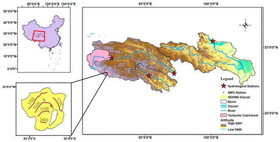
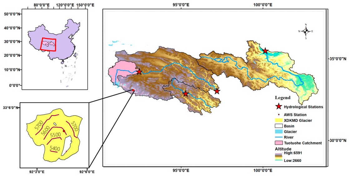
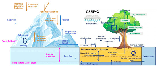
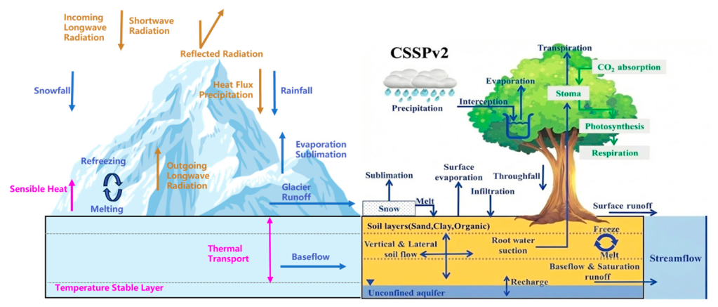
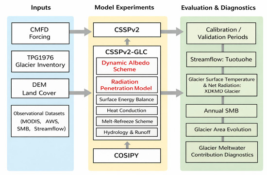
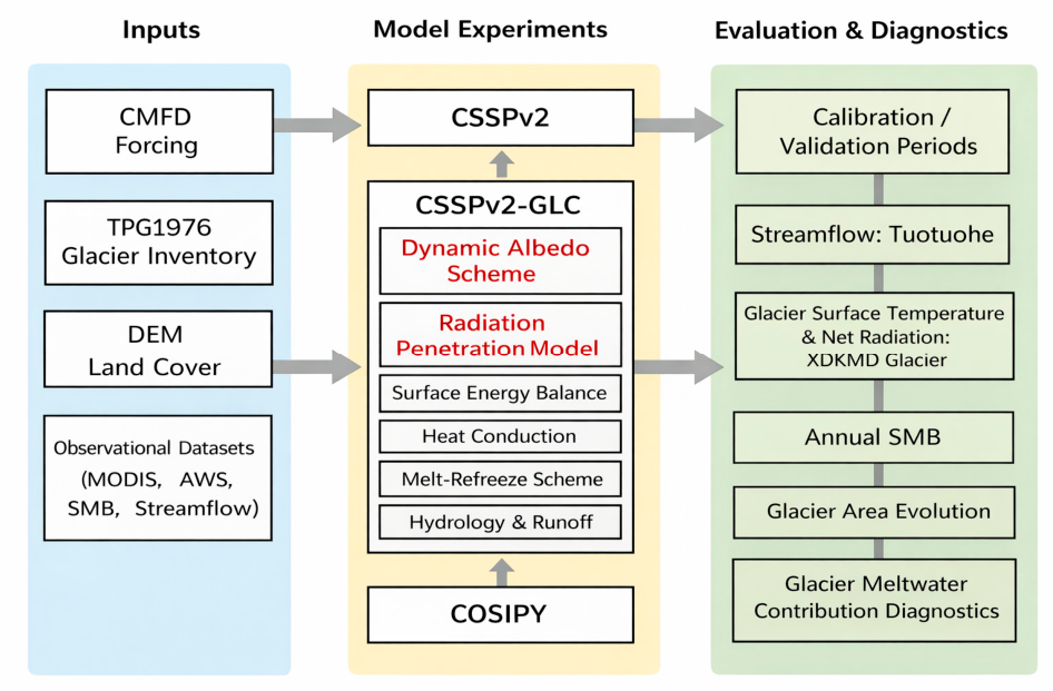
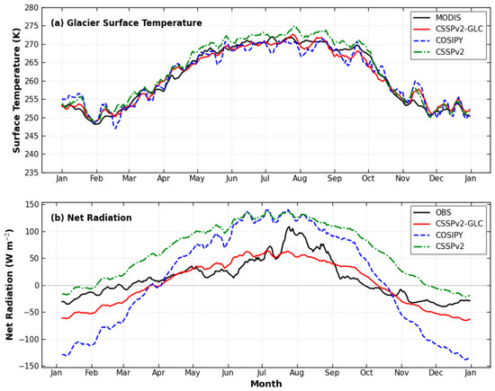
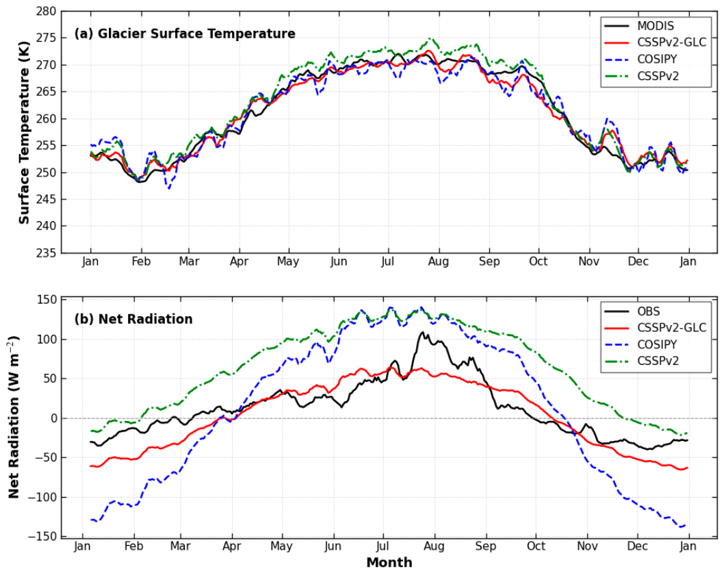
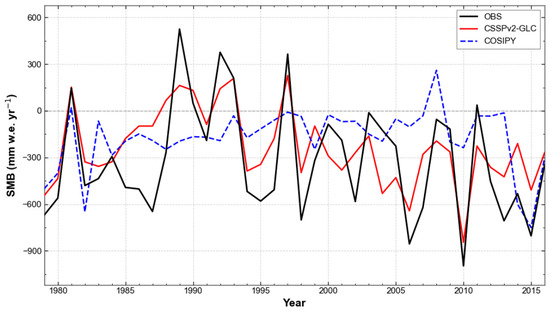
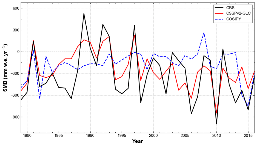
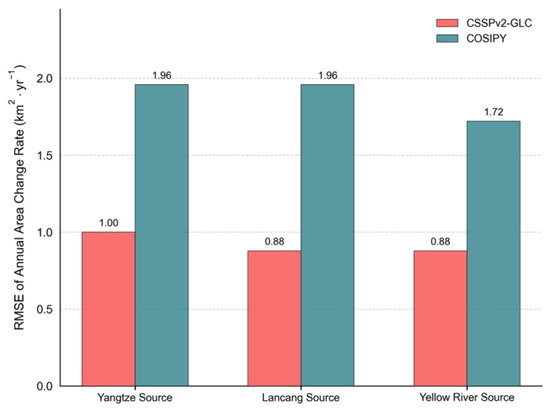
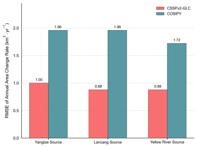
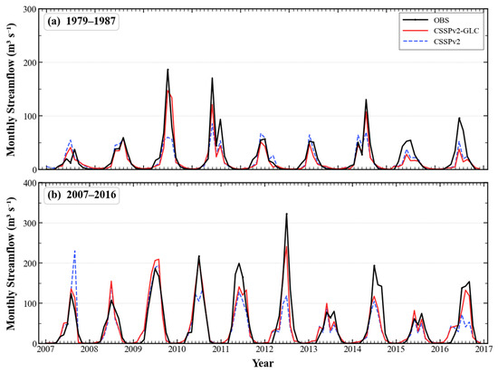
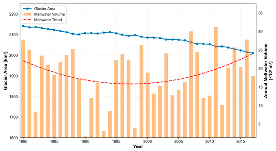
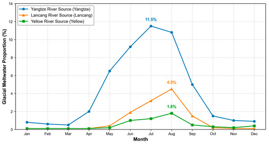
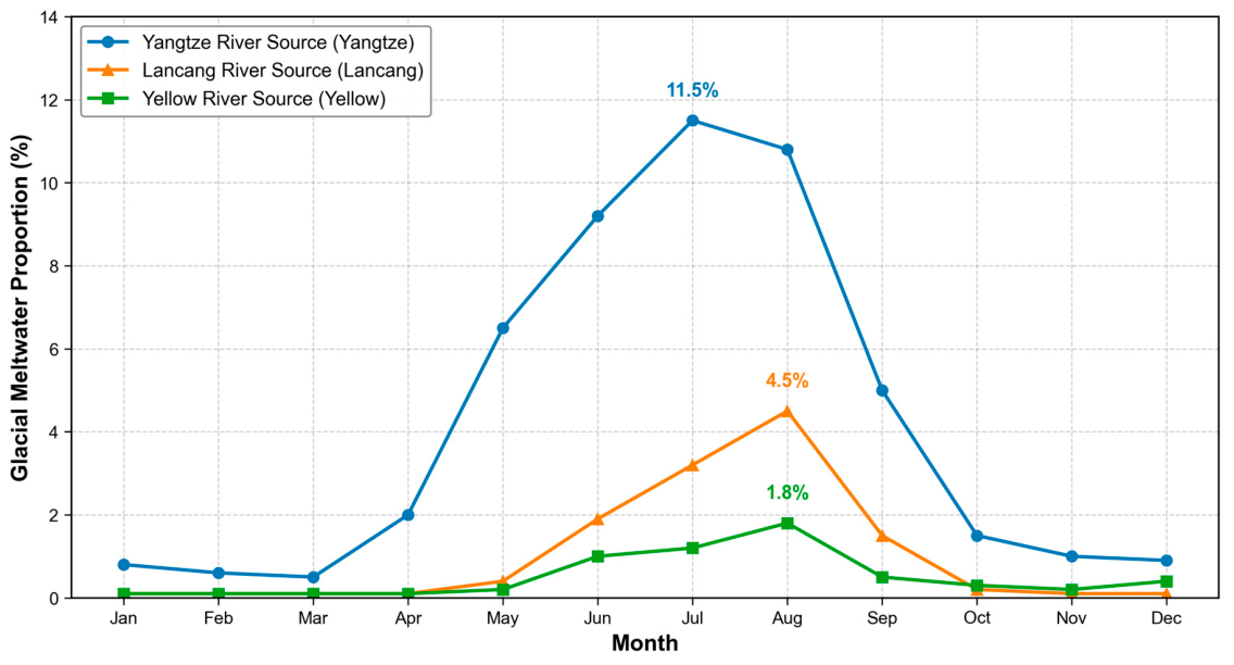
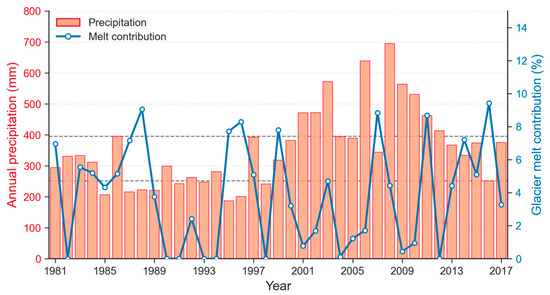
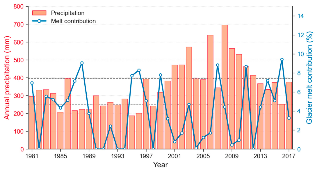

Disclaimer/Publisher’s Note: The statements, opinions and data contained in all publications are solely those of the individual author(s) and contributor(s) and not of MDPI and/or the editor(s). MDPI and/or the editor(s) disclaim responsibility for any injury to people or property resulting from any ideas, methods, instructions or products referred to in the content. |
© 2026 by the authors. Licensee MDPI, Basel, Switzerland. This article is an open access article distributed under the terms and conditions of the Creative Commons Attribution (CC BY) license.