Estimation of the Mean-to-Surface-Velocity Ratio in Shallow Streams with Rough Beds

Abstract

Estimating in a stream’s cross-section the depth-averaged velocity, V, from the free-surface velocity, v_surf, is an efficient, non-invasive hydrometric method. The ratio f_v = V/v_surf is typically assumed constant at f_v = 0.86 in field applications, despite observations to the contrary. Guidance is, therefore, needed in estimating actual f_v-ratios when velocity profile data are absent. This work provides field-verified guidance based on the hydromechanics of the logarithmic velocity law, which shows that f_v depends on the scaled resistance measure ‘friction length/depth’, y_o/h, with the y_o(k) function of the equivalent sand grain roughness, k. The mean-to-surface-velocity ratio in rough-bed streams is estimated from the bed roughness and stream morphology by modifying Nikuradze’s equation, y_o = k/30, to y_o = ck, with c(h/k) ≥ 1/30, and k ≈ D₈₄—data fit: c ≈ 8.61(h/k)^−1.821, ~5 ≤ h/k < ~30. Field-verification of the ratio’s modified hydromechanics, f_v = f$\left(h/y_o\right),$ with y_o(h/k) evaluated from bed roughness estimated by inspection or sieve analysis shows this ratio holding within ~|10|% error for shallow streamflow over a coarse bed of gravels and rocks, giving submergences of ~5 ≤ h/D₈₄ ≤ ~30; y_o = k/30 suits large streams with smooth beds (h/k ≥ ~30, f_v ≥ ~0.86). Variable roughness-estimated f_v-ratios appear to be more reliable than the fixed default, f_v(h/y_o ≈ 1000) = 0.86. This flow-gauging concept is based on observable physical characteristics of a monitoring cross-section and facilitates the rating of hard-to-access streams draining small basins in ragged upland terrain.

1. Introduction

Streamflow is the paramount quantity in surface hydrology, so considerable attention is paid to its monitoring, yet observations have decreased consistently since the 1980s [1]. Discharge through a stream’s cross-section is monitored operationally by converting observed stages, h, to flows, Q, via a rating curve, Q(h). Streamflow, however, is monitored regularly only in large rivers; in small streams, rating curves are often absent [2]. A rating curve is constructed by integrating velocities sampled in a cross-section of known bathymetry over a range of flows, ideally up to flood flows. However, practical issues exist; e.g., in-stream point-sampling with a current meter can be dangerous even at non-extreme flows (rule of thumb limit: velocity(m/s) × depth(m) ≤ ‘1’) and is prohibitive at high flows. In contrast, a fixed side-looking Acoustic Doppler Current Profiler (ADCP), which measures speed from the frequency shift (Doppler effect) of a transmitted signal scattered back to the transceiver through particles in the water [3], is safe but too expensive and often unsuitable for routine use in small, shallow streams [4], which may be also difficult to access. A portable ADCP can also be employed in shallow streams via wading; however, the hydrographer is again exposed to high-velocity risks. Rating curves are thus often extrapolated to high flows, despite such extrapolations being prone to significant errors.

Measuring velocities on the free surface of a stream can be a suitable hydrometric alternative if surface velocities can be related to depth-averaged velocities at the sampling locations. This approach rests on the ability to sense surface velocities remotely. Image velocimetry (e.g., Refs. [5,6,7,8]) and hand-held radar [9] allow us to carry out such non-invasive observations efficiently. Estimating the mean velocity, V, as a constant fraction. f_v, of the surface velocity,$v$_surf, V = f_v $v$_surf, is convenient. The default value, f_v ≈ 0.86 [10], fits a logarithmic velocity profile with the dispersion quantified by the momentum distribution coefficient β = 1 + (σ/μ)² ≈ 1.03, σ/μ ≈ 0.16; μ = V is the profile’s mean velocity and σ its standard deviation [11]; a power-law velocity profile with the exponent m = 6 also yields f_v = m/(m + 1) ≈ 0.86. Through hydraulic reasoning, however, a constant f_v-ratio is an approximation [12], and its variability with the discharge has been observed in the field, e.g., at the gauging station of a large river [13]. Analysis of 3611 streamflow datapoints from mostly medium to small French rivers (in 90% of cases: Q < 10.2 m³/s, hydraulic radius: R_h < 0.63 m, and width: b < 24.8 m) found f_v-values ranging from ~0.7 to 0.95 (5% to 95% quantiles) [14]. A large set of streamflow records from rivers across the USA was evaluated (mean values: Q = 483 m³/s, top width: B = 94.4 m, and depth: h = 2.32 m) in [15], cf. figure 2b, and significant variability in the maximum-to-mean-velocity ratio was found. At gauging stations on the Tiber River, f_v-ratios ranged in the interval 0.86 (wide section) ≤ f_v ≤ 1.05 (narrow section, profile dip) [16], while [17] found V/v_max ≈ 0.7 in three streams.

However, f_v-values generally vary also across a stream, particularly in upland catchments, due to the variable depth and bed roughness in irregular natural cross-sectional geometry; the relative roughness (=roughness/depth) thus varies across the stream. The logarithmic velocity profile (see Section 2) has been used in [13] to show that f_v is a function of the ratio friction length/depth, and, since the friction length depends on the roughness, the relative roughness is generally variable, and so is the f_v–ratio. This reasoning, supported by the data mentioned above, as well as by observations such as those in appendix C in [18], and [19] and also of the authors of [11], motivated this reassessment of the hydromechanics underpinning the f_v-ratio.

The emphasis here is on streamflow in shallow channels with rough beds. Accepting the logarithmic law, we modify the friction length from Nikuradze’s original value [20,21,22], relating it to the relative roughness, to fit the flow conditions in shallow channels with rough beds. The key to this work is determining f_v-ratios by estimating relative roughness from sampling/observations of the bed material and from the bathymetry of smaller streams with irregular cross-sections and rough beds. We use field-verified hydromechanics to estimate the mean-to-surface-velocity ratio when velocity profile data are absent, aiming to provide the guidance that hydrographers lack. Then, gauging the discharge from surface velocities would especially facilitate setting up rating curves at difficult-to-access ungauged streams with rough bed draining small basins in ragged upland terrain.

2. Concepts and Fundamental Equations

In the absence of a measured discharge, or of at least a measured velocity profile, an analytical model of the velocity variation in an open channel must be used in order to estimate an f_v-ratio that parameterizes the conversion of surface velocity to depth-averaged velocity. Such analytical models idealize steady free-surface streamflow as fully developed (longitudinally uniform) in an infinitely wide channel (2-D). Assuming an infinitely wide channel is a major approximation, as the velocity field in natural streams depends on cross-sectional shape and roughness. However, also traditional hydrometry applies quasi-2D analysis: it assumes a streamflow field as represented by velocities sampled at verticals on which the selection of sampling points is guided by the Prandtl–von Kármán logarithmic velocity profile in an infinitely wide channel, at 60% of a shallow (≤0.76 m) depth below the free surface, or at 20% and 80% or at 20%, 60% and 80% of depth; a midsection’s mean velocity is obtained by weighing the observations appropriately [3].

The Prandtl–von Kármán logarithmic law [20,21,22] and the mathematically simpler, but empirical, power law [20] are often used to fit measured velocities [9,23], doing so about equally well (as does the parabolic profile of [17]). The logarithmic law has been selected for this analysis because its parameters are observable, while the power-law exponent is not; see also [24].

The logarithmic Prandtl–von Kármán velocity law describes steady, uniform turbulent flow in an infinitely wide channel (approximately in channels of finite width, b, and depth, h, with h/b << 1):

$$v\left(y\right) = (v_{*}/\kappa ) \mathrm{l}\mathrm{n}\left(y/y_o\right), { y}_o\le y\le h$$

(1)

$v_{*}$ is the shear velocity, κ ≈ 0.4 is the von Kármán constant (clear water), and y is the normal distance from the bed; the friction length, $y_o$, positions the zero-velocity, $v\left(y_o\right)=0$, evading the logarithm’s infinite tail at zero [20,21,22]. The logarithmic law is derived by approximating the shear stress near the wall as constant (Prandtl’s mixing length model, l = $\kappa y$ [25]) but has been found to also describe the velocity profile well in the outer region [26]. The shear velocity, $v_{*}$ = $\sqrt{{\tau }_o/\rho }$ (ρ is the water density), expresses the wall shear, τ_o, i.e., the resistance force that macroscopically balances the gravity force in steady uniform flow. The derivative of Equation (1), dv/dy = $(v_{*}/\kappa )/y$, shows that the variation in the velocity increases with increasing bed resistance (higher ${ v}_{*}$) and decreases with increasing depth. Hence, velocity profiles over smooth beds in deep cross-sections, common to large rivers, are expected to be fairly uniform, i.e., high f_v. Conversely, velocity profiles in shallow streams with rough beds, common to headwaters, are expected to be more variable, i.e., low f_v.

According to Nikuradze’s [27] flow experiments on pipes, $y_o$ depends on the turbulence level and the wall roughness, except in the hydraulically smooth regime, where the roughness elements are submerged in the viscous sublayer, y_o = ν/9$v_{*}$, and ν is kinematic viscosity (e.g., [28], p. 201); such conditions may occur in certain laboratory settings and commercial pipes, but they rarely exist in natural streams. Nikuradze gives the friction length in hydraulically rough flow as a fixed fraction of the equivalent sand grain roughness, k, which he defines using the median grain diameter, D₅₀:

y_o = k/30.

(2)

This result holds for the roughness type and range of Nikuradze’s [27] experiments, in which sand grains of nearly uniform diameter, packed in the densest formation, were glued to an inner pipe wall [22] so that only a sector of those ‘spherical’ grains protruded above the glue layer into the flow. The large size of natural channels gives high Reynolds numbers, R = V(4R_h)/ν ≥ 10⁵–10⁶ (R_h is the hydraulic radius, and ν ≈ 10⁻⁶ m²/s is the kinematic viscosity of water), which, combined with a fairly rough wetted perimeter, for example, a relative roughness of k/(4R_h) ≥ 0.01, places the flow in the hydraulically rough regime, where resistance depends on the relative roughness alone [21,22,26]. Nikuradze’s relationship, however, must likely be modified for shallow channels with rough granular boundaries. Tentative results from Smart (reported in [18,19]) show that f_v decreases markedly for submergence values of h/D₈₄ < 10; h/D₈₄ is an inverse relative roughness measure, with D₈₄ the size of the 84th largest percentile of the grains of the bed material. The authors of [29] report similar results.

According to the Prandtl–von Kármán logarithmic law, f_v varies with the relative roughness length = y_o/(depth h) [13], and experiments by [29] using a laboratory flume demonstrate that V/$v$_max (log-profile: $v$_max = $v$_surf) depends on the submergence, h/k. The observed variability of f_v with discharge [13] is explained by the variation in relative roughness with depth, while the inherent variability of f_v across a natural stream is acknowledged in [18]. In ref [13], an ensemble profile was formed from velocity data sampled at several verticals, from which they extracted a cross-sectional f_v–value by fitting a log-profile to the normalized data ensemble; this method weighs profiles equally and suits streams of fairly uniform cross-sectional characteristics. An over-the-cross-section average f_v-value was also used in [9]. A key idea in our work is to determine local f_v-ratios by estimating variable relative roughness from bathymetry and by sampling or observing the bed material of smaller streams with irregular cross-sections and rough beds: f_v = f(k/h).

3. Review of the Hydromechanics of the Surface Velocity to the Depth-Averaged Velocity Ratio

3.1. The Equations of Hydromechanics, with Laboratory and Field Evidence

The presence of two parameters, $v$_* and y_o, makes the logarithmic law appear unsuitable for a parsimonious discharge estimation. However, upon forming the ratio of the mean velocity to the surface velocity, f_v =V/$v$_surf (Equation (5), below), the friction velocity is eliminated, and the only parameter remaining to be estimated is the friction length.

The profile’s mean velocity, V, is obtained by integrating Equation (1) over the nominal water column, from y_o to the free surface at y = h,

$$V=\left({\displaystyle \frac{v_{*}}{\kappa }}\right)\left[{\displaystyle \frac{h}{h{-y}_o}}\mathrm{l}\mathrm{n}\left({\displaystyle \frac{h}{y_o}}\right)-1\right],$$

(3)

and the surface velocity is given by evaluating Equation (1) at y = h,

$$v\left(h\right)=(v_{*}/\kappa ) \mathrm{l}\mathrm{n}\left(h/y_o\right).$$

(4)

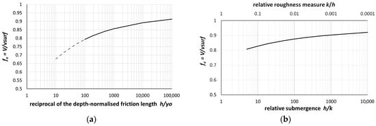
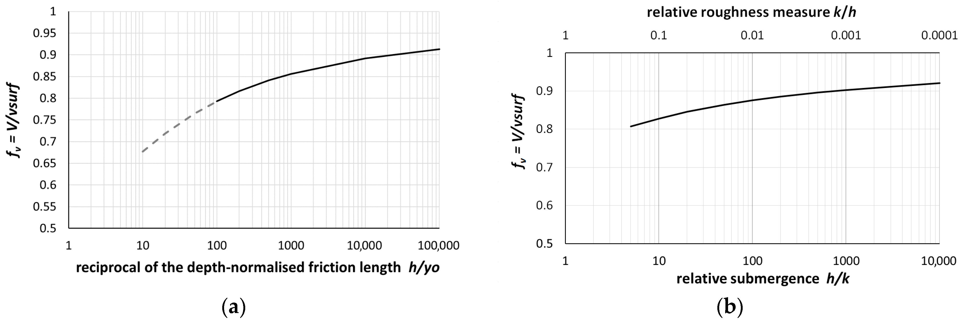
Dividing Equation (3) by Equation (4) gives the f_v-ratio as a function of $h/y_o$, as already derived by Le Coz et al. (2010) [13] and graphed in Figure 1a,

$$f_v=V/v_{\mathit{surf}}={\displaystyle \frac{h}{h{-y}_o}}-1/\mathrm{l}\mathrm{n}\left(h/y_o\right)={\displaystyle \frac{1}{1-y_o/h}}-{\displaystyle \frac{1}{\mathrm{l}\mathrm{n}\left(\frac{h}{y_o}\right)}},$$

(5)

(f_v ≈ 1 +${ y}_o$/h $-1$/$\mathrm{l}\mathrm{n}\left(h/y_o\right)$ for h/$y_o$ ≥ 100, error < 1%); typical values of the reciprocal of the depth-scaled friction length in streams are 10² ≤ h/y_o ≤ 10⁴ [13]. Equation (5) may be the basis for a parsimonious discharge estimation, provided that the friction length is linked to the bed roughness across the h/y_o-range of interest, so that V/$v$_surf is quantified as f_v(k/h); this is shown in Figure 1b for Nikuradze’s y_o = k/30, per Equation (2). Further, the logarithm in Equation (5) ‘forgives’ misestimating y_o by compressing uncertainties about the roughness.

Figure 1. fv = V/$v_{\mathit{surf}}$ as a function of (a) h/y_o, Equation (5), and (b), again with Equation (5), and for y_o = k/30, based on the Prandtl–von Kármán log-profile for uniform turbulent flow in an infinite-width channel.

As mentioned above, the laboratory experiments in [29] demonstrate that ϕ = V/$v$_max (for log-profile, $v$_max = $v$_surf) depends on the submergence. h/k. (NB: In pipe flows, the roughness scales with the hydraulic diameter, D_h = 4R_h, i.e., k/4R_h (≈k/4d in shallow channels, h/b << 1); therefore, the reciprocal of the submergence is four times the relative bed roughness, 4k/(4R_h) ≈ 4k/4h = k/h, in an infinitely wide channel.) Drawing on additional laboratory and field data, Greco and Martino [29] developed an empirical graph, ϕ(h/k), similar to Figure 1b but somewhat simplified. It consists of two straight lines: the horizontal, ϕ = 0.9, corresponds to beds with h/k ≥ 20, while for 2 < h/k < ~7 (quite rough beds), ϕ varies in the range 0.52–0.73; the intermediate zone, ~7 < h/k < ~30, is nearly unpopulated (the graph has a gap).

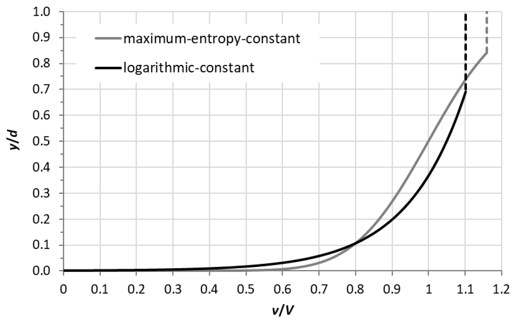
Field data in [13,14] (also citing a flume study) show that the logarithmic profile fits streamflow up to y/h ≈ 0.65, above which the data are approximated by a constant velocity. Koussis et al. [11] truncated a maximum-entropy (ME) velocity profile at y/h = 0.84 and fitted the constant velocity v_surf = v_ME(0.84) = V + σ above it; as it turns out, v_ME(0.84) = v_log(y/h = 1) (see Figure A1 in Appendix A for the log-constant and max-entropy-constant profiles). The authors of [17] found the $v$_max located at 0.71 ≤ y/h ≤ 0.8. Equation (6) (analogous to Equation (5)) was derived for the log-constant profile in [13], for which, typically, η = (y/h)_dip ≈ 0.6–0.7:

$$f_v = V/v_{\mathit{surf}} = {\displaystyle \frac{h}{h{- y}_o}}- {\displaystyle \frac{\eta h{- y}_o }{h{- y}_o}}1/\mathrm{l}\mathrm{n}\left(\eta h/y_o\right)$$

(6)

Values of h/y_o resulting from fitting a logarithmic profile to all observations and just to data of the logarithmic part of a log-constant profile are different, but only the friction length of the former has physical meaning [13]. Obviously, Equations (5) and (6) yield different values of h/y_o for the same f_v-value, with the log-constant profile indicating an apparently reduced friction length.

Biggs et al. [18] developed an equation that brackets the f_v-ratio estimates at ungauged sites from the bed slope, S_o, from the logarithmic law. Equation (4), solved for the friction length and substituted in Equation (5), gives

$$y_o=h/\exp (\kappa v_{\mathit{surf}}/v_{*}),$$

(7)

$$f_v=V/v_{\mathit{surf}}={\displaystyle \frac{h}{h{-y}_o}}-1/\mathrm{l}\mathrm{n}\left(h/y_o\right)={\displaystyle \frac{1}{1-\mathrm{e}\mathrm{x}\mathrm{p}\left(-\kappa \frac{v_{surf}}{v_{*}}\right)}}-{\displaystyle \frac{v_{*}}{{\kappa v}_{surf}}}.$$

(8)

The macroscopic momentum balance in the flow direction for uniform flow in an infinitely wide channel, ${\tau }_o$= $\rho g{S}_o,$ and the definition of the shear velocity, $v_{*}$ = $\sqrt{{\tau }_o/\rho }$, give $v_{*}$ = $\sqrt{gh{S}_o}$; S_o = sinθ, with θ the bed’s angle against the horizontal. Entering that result into Equation (8) eliminates the shear velocity and expresses the flow ratio in terms of the bed slope:

$$f_v = V/v_{\mathit{surf}} = {\displaystyle \frac{1}{1- \mathrm{e}\mathrm{x}\mathrm{p}\left(-\kappa \frac{v_{surf}}{\sqrt{gh{S}_o}}\right)}}-{\displaystyle \frac{\sqrt{g{hS}_o}}{{\kappa v}_{surf}}} .$$

(9)

This f_v estimator trades off the uncertainty about the friction length in y_o/h for the approximation of the friction slope by the bed slope that is assumed to hold under all flow conditions. Related drawbacks are (a) profiles in streams that may not be logarithmic (applies to either method), (b) a friction slope that generally differs from the bed slope, and (c) roughness that is not considered explicitly.

3.2. Flow Conditions in Shallow Channels with Rough Granular Boundaries

If flow conditions resemble those in Nikuradze’s lab experiments (uniform k/h << 0.1), estimates of y_o from Equation (2) likely yield plausible f_v-values. The equivalent sand grain roughness and the shear velocity appear in the wall Reynolds number, R_w = $v_{*}$k/ν, which classifies resistance in boundary layer flow: R_w < 4 hydraulically smooth, R_w > 100 hydraulically rough, and 4 < R_w < 100 the transition zone [30]. On the other hand, if the bed in a shallow stream is coarse, the data in [17,29] indicate f_v < ~0.7, which translates, via Equation (5), to h/y_o ≤ ~20 and then via Nikuradze’s Equation (2), y_o = k/30, to the uncommonly extreme h/k ≤ ~2/3. We therefore argue, in analogy to the work in [31,32] on flow resistance in streams with rough gravel beds, that a relationship different from Equation (2) is appropriate for estimating the friction length from a bed-material roughness size for, e.g., h/k < ~6, assuming k = D₈₄, or for h/k < 10, assuming k = D₅₀. These limits exceed the top of the intermediate roughness scale of [33] by ca. 1/3, defined as 1.2 < h/D₈₄ < 4 or 2 < h/D₅₀ < 7.5.

Various statistical roughness measures of the form k = aD_x, a ≥ 1 and x percent finer than D define k in this range of natural roughness in the literature. In [18], Smart characterized the roughness regime via h/D₈₄, and Greco and Martino [29] used h/D with D the diameter of sand grains forming the bed plus the diameter of the spheres fixed on it. In [27,34,35,36] h/D₅₀ was chosen. In [32] gravel-bed roughness was characterized with D₈₄, a size compatible with the observation that the bed of natural streams tends to be armored with the larger roughness elements ([30], Chapter 10). The h/D values in [29] are somewhat smaller than h/D₈₄; however, the two measures are comparable because the spheres are identical and the sand grains d_g << D; in those rough-bed experiments, h/D falls in the intermediate to the rough scales, 1.89 ≤ h/D ≤ 6.43, which explains values of V/v_max (≈f_v) in the range 0.52–0.73. Fairly large ranges of h/D₈₄ are assigned to single f_v-values in table 4.2 in [18]; e.g., 10 < h/D₈₄ < 30, f_v = 0.84, and 2 < h/D₈₄ < 10, f_v = 0.63; therefore, these correspondences to the roughness classification of [33] are quite approximate.

In principle, the bed roughness can be characterized on the basis of the standard deviation, σ_bed, of the distance from a reference plane to the top of a solid boundary’s granular elements [37] (an approach appropriate for laboratory research but impractical for field work). Monzavi’s method was applied in flume experiments of free-surface flow over a permeable rough bed of 20 mm average-diameter natural gravel in [38], and σ_bed = 7.83 mm was determined as the roughness; the submergence was calculated as H_o/σ_bed, with H_o = flow depth + σ_bed the nominal depth above the reference level, for two runs with depths h = 7.5 cm and 9.2 cm: H_o/σ_bed = 10.58 and 12.75, respectively.

4. Estimation of the f_v-Ratio in Rough-Bed Channels Based on the Relative Roughness

The velocity profile over a rough bed is linear in the thin laminar sublayer, logarithmic in the turbulent boundary layer above it, and slightly non-logarithmic in the outer layer [26]. In low-submergence flows, however, the velocity profile may deviate from the logarithmic form; nevertheless, several studies reported in [31] show that log-based resistance equations still afford adequate predictions. For irregular, large macro-scale roughness, Nikuradze’s roughness height (for hydraulically rough flows in pipes with inner walls covered with near-uniform sand grains) is not a suitable lower integration limit for the log-profile, as data show that this profile does not extend over the depth, h. A zero-displacement, d₀, was introduced in [35] to parameterize the space-and-time-averaged logarithmic profile, v(y) = $\left({\displaystyle \frac{v_{*}}{\kappa }}\right)$ln[(y − d₀)/(y_low − d₀)] + v_slip, from y_low, v(y_low) = v_slip ≠ 0, to y_high < h; this equation has a solid hydromechanics basis but is too complex for hydrometric practice. Therefore, we modify the f_v-relationship derived from the logarithmic law to apply it down to the start of the intermediate roughness range, with the generalized friction length expression

y_o = ck, variable c ≥ 1/30 and k ≈ D₈₄

(10)

such that Equation (10) fits the data in [29] well and that of Smart (in [18]) for ~5 ≤ h/D₈₄ ≤ ~10, merging smoothly with Equation (5) at h/k = 33 (Nikuradze’s y_o = k/30, f_v ≈ 0.86):

$$f_v = V/v_{\mathit{surf}} = {\displaystyle \frac{h}{h{- y}_o}}- 1/\mathrm{l}\mathrm{n}\left(h/y_o\right)={\displaystyle \frac{1}{1- ck/h}}-1/\mathrm{l}\mathrm{n}\left(h/ck\right)$$

(11)

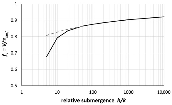
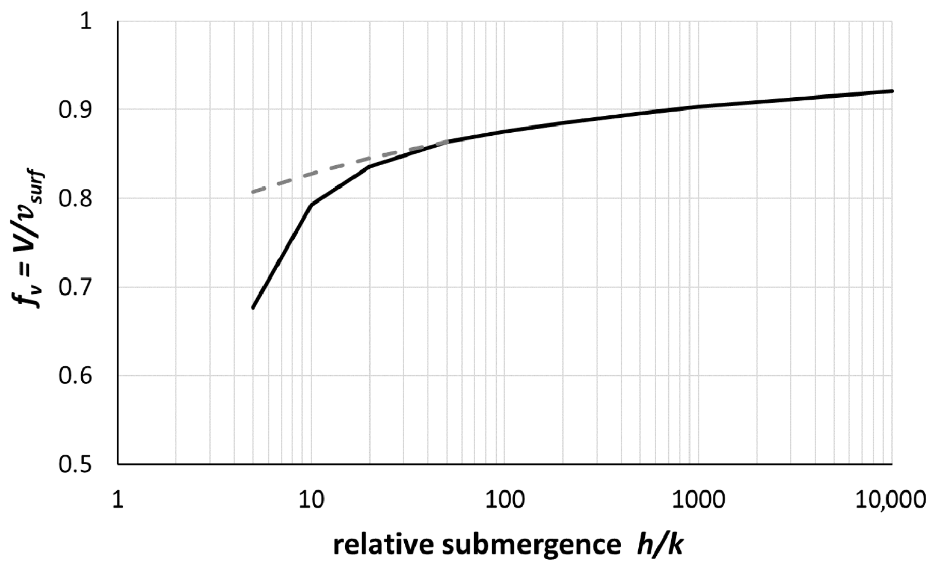
Figure 2 shows Equation (11) with c = 0.013 at h/D₈₄ = 33, c = 0.05 at h/D₈₄ = 20, c = 0.1 at h/D₈₄ = 10 and c = 0.5 at h/D₈₄ = 5, which yield f_v = 0.86, 0.836, 0.793 and 0.677, respectively; c = 0.013 derives from Nikuradze’s c = 1/30, after adjusting the k from D₅₀ to D₈₄ by assuming an exponential distribution. These (c, h/D₈₄)-data are regressed by the relationship

c = 8.61(h/D₈₄)^−1.821, r² ≈ 0.973, ~5 ≤ h/D₈₄ ≤ ~33

(12)

Figure 2. Ratio f_v = V/v_surf = f(h/k) based on log-profile: Equation (11) with c(h/D₈₄); Equation (11) with c = 1/30.

Increasing friction lengths are reflected in larger c-values as h/D₈₄ decreases, particularly for h/D₈₄ < 10, accounting, approximately, for the prominent form drag in the total resistance [21,26] in shallow flow over a rough bed [33]. The findings of [38], that logarithmic profiles fit the data in their two aforementioned runs with the equivalent sand grain roughness multiplied by 1.5 to 2, i.e., c = 0.05–0.067, are relevant in this context. In Section 4, we test Equations (10)–(12) with field data. We remind the reader that the constants in the log-profile, $v\left(y\right)/v_{*} = 2.5\mathrm{l}\mathrm{n}\left(y/k\right) + 8.5$, derive from y_o = k/30 and κ⁻¹ = 2.5 (8.5 = 2.5ln30) and should be adjusted in the case of fairly rough walls.

The sensitivity, S, of the f_v-ratio to variation (or to misestimation) in the roughness, k, is S = df_v/dk = (df_v/dy_o)(dy_o/dk), with y_o = c(k)k = N(h/k)^ζ k, N = 8.61 and ζ = −1.821, Equations (11)–(12). Evaluation of this expression gives S = {h⁻¹(1 − y_o/h)⁻² − y_o⁻¹[ln(y_o/h)]⁻²}[N(1 − ζ)(h/k)^ζ], which is restated as

S = {(y_o/h)(1 − y_o/h)⁻² − [ln(y_o/h)]⁻²}[N(ζ − 1)/k] = F(y_o/h)/k

(13)

The function, F, on the right-hand side of Equation (13) is F(y_o/h) = F(k/h); hence, given k/h and Δk, Δf_v = F(k/h)Δk/k. We consider, as an example, the case k/h = 0.1, f_v ≈ 0.79; if k = 0.05 m and Δk = 0.01 m, Δk/k = 0.2 or 20%, and then Δf_v ≈ 0.03 and Δf_v/f_v ≈ 4%; i.e., the uncertainty in estimating the roughness, k, causes a lesser uncertainty in f_v, and thus in estimating the discharge.

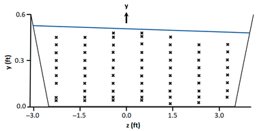
Before applying the method in the field, we prove the concept with high-accuracy data in [39] that were sampled nearly uniformly in the laboratory channel of a trapezoidal cross-section, with a base width of b_b = 6 ft (1 ft = 0.305 m), a depth across the base of h ≈ 0.5 ft (the free surface is tilted due to the meandering flow) and side slopes of 1:1. The Cartesian co-ordinates are indicated in Table 1, which lists the observations shown as velocity profiles in Figure 3. The channel’s meandering course induced a spiral secondary flow in the trapezoidal cross-section that was more pronounced than would have been solely due to finite width and inclined sides; this is contrary to the uniform longitudinal flow in the infinite-width cross-section assumed in the 2-D-flow theory.

Table 1. Velocities (ft/s) measured in a trapezoidal cross-section (Yen, 1965, [39]).

	0.4750	-	-	3.737	3.737	-	-	-
	0.4500	3.140	3.611	3.721	3.705	3.548	-	-
	0.4000	3.218	3.595	3.642	3.699	3.548	3.266	2.779
	0.3500	3.250	3.548	3.611	3.674	3.564	3.266	2.889
	0.3000	3.281	3.454	3.564	3.580	3.548	3.297	2.967
	0.2500	3.297	3.423	3.454	3.517	3.485	3.328	2.999
	0.2000	3.266	3.375	3.375	3.423	3.454	3.328	3.048
	0.1500	3.203	3.313	3.281	3.344	3.344	3.288	3.030
	0.1000	NaN	3.234	3.203	3.203	3.234	3.140	2.952
	0.0500	2.889	3.014	3.014	3.014	3.014	3.014	2.828
	0.0250	2.795	2.857	2.795	2.905	-	-	-
	0.0125	-	-	-	-	2.822	2.590	-
	depth (ft)/ distance (ft)	−2.35	−1.40	−0.45	0.50	1.45	2.40	3.35
	verticals	1	2	3	4	5	6	7

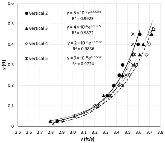
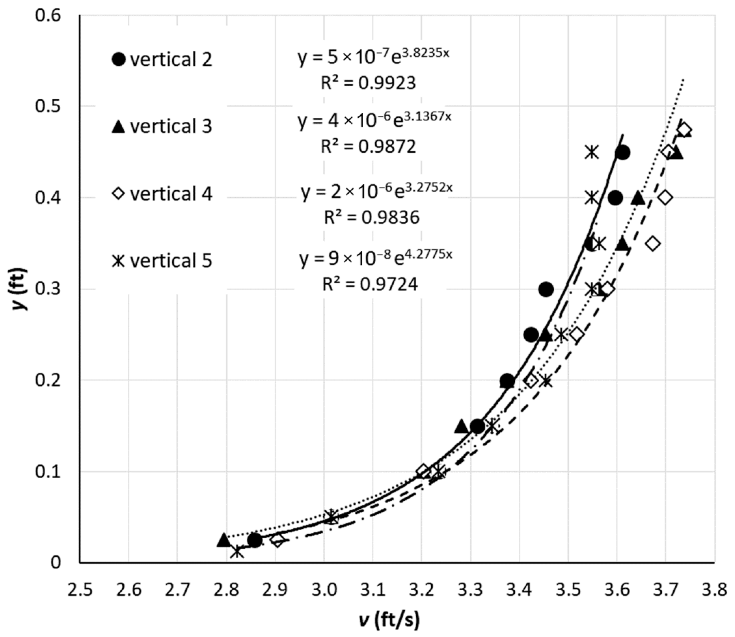
Figure 3. Velocity data and log-profiles in the trapezoidal cross-section of a laboratory channel.

The profiles measured on the verticals at z = −1.40, −0.45 and 0.5 ft conform very well to the logarithmic law idealization (r² ≈ 0.98), with friction lengths of 5 × 10⁻⁷ ft ≤ y_o ≤ 4 × 10⁻⁶ ft (1 ft = 0.305 m); the two central profiles give y_o ≈ 3 × 10⁻⁶ ft. The profile at z = 1.45 ft is log-constant, while the profiles at z = −2.35, 2.40 and 3.35 ft exhibit a maximum below the free surface (a dip) (see Table 1). The texture of the solid boundary is ‘well finished cement mortar’ ([39], p. 32), for which ([22], table 8.3.5.1) lists k in the range 0.012–0.170 mm; we use k = 0.1 mm (~average). Then, y_o = k/30 gives y_o ≈ 1.1 × 10⁻⁵ ft, so h/y_o ≈ 4.575 × 10⁴ and, via Equation (5), f_v = 0.906. The log-profiles on the two central verticals fit the data with y_o ≈ 3 × 10⁻⁶ ft, so h/y_o ≈ 1.67 × 10⁵ and f_v ≈ 0.916. The flat f_v-curve for h/y_o ≥ 10⁴, Figure 1a, explains the close agreement of these f_v estimates. Evaluation of the raw data on the two central verticals gives f_v ≈ 0.91. The resistance regime for equivalent sand grain roughness, k = 0.1 mm and κ/$v_{*}$ ≈ 3.2 s/ft (see Figure 3), with ν = 1 × 10⁻⁶ m²/s$, v_{*}$ ≈ 0.125 ft/s ≈ 0.038 m/s, is borderline smooth-transitional, R_w = $v_{*}$k/ν ≈ 4, which also explains f_v ≈ 0.9.

The validity of the proposed concept is supported by the agreement, within ~1%, of the mean to the surface velocity ratios based on the raw data and derived using Equation (5) with the friction length estimated: (a) from the observed (central) velocity profiles and (b) according to Nikuradze’s Equation (2) by adopting the value of the equivalent sand grain roughness from a table. These results are also fair, given that the flow was meandering in this trapezoidal channel (non-2D, h/b ≈ 1/12). Considering only the logarithmic part of the non-logarithmic profile on the off-center vertical, z = 1.45 ft (near-vertical for y > 0.35 ft, η ≈ 0.7, Figure 3, like those observed in [13]), yields the (lacking physical meaning) apparently reduced friction length, y_o = 1 × 10⁻⁶ ft (one-third of the estimates from the central log-profiles); Equation (5) then gives f_v ≈ 0.925 (little changed, due to the flat f_v-curve for h/y_o > ~10⁴, relative to f_v = 0.916 derived from the profiles on the central verticals). But if, for comparison, Equation (6) is applied with h = 0.5 ft, η = 0.7 and the inconsistent value, y_o = 1 × 10⁻⁶ ft, the estimate is f_v ≈ 0.95, while y_o = 3 × 10⁻⁶ ft gives f_v ≈ 0.94; these inconsistent results overestimate the ratio f_v = 0.916 from the observed data of the central profiles by ca. 3% and that from the raw-data-derived f_v ≈ 0.9 by almost 5%. In any case, however, f_v ≠ 0.86.

5. Field Applications of the Velocity Ratio V/v_surf = f(h/(ck)) in Open-Channels with Rough Bed

The procedure for applying the proposed methodology first consists of preparation: (a) ascertain the bathymetry from the water level and the cross-sectional geometry, and (b) estimate the roughness by either inspecting the stream bed, or better, through sieve-analysis of the sampled bed material. It then involves operation: measure (i) the stage and (ii) the surface velocity (remotely, e.g., with hand-held radar) at a number of positions to capture the lateral velocity variation, considering the variable macro-geometry, h, and bed roughness k, and (c) use Equations (11) and (12) to calculate f_v and V = f_v$v$_surf.

First, however, we assess how Equation (11) for f_v(k/h) applies in the field using streamflow data from monitoring stations in the Peloponnese, Greece: (i) at Atsicholos Bridge on the river Loussios, near Karytaina, Arcadia; (ii) near Karavas village, Laconia, on the Evrotas River; and (iii) at the Rentifi Mill on Alagonia Creek, Messinia. Detailed velocity profiles sampled with a current meter are used for verification; the data are stored in the database HYDRONET [40], https://hydronet.noa.gr (accessed on 17 January 2024), established in the OpenHi.net project [41]. The bed material was inspected carefully while recording the bathymetry of the monitoring cross-sections. The quality characteristics of the log-profiles fitting to the data are listed in the Supplementary Material B.

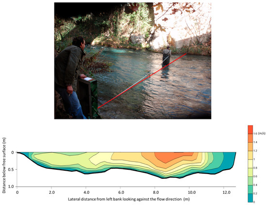
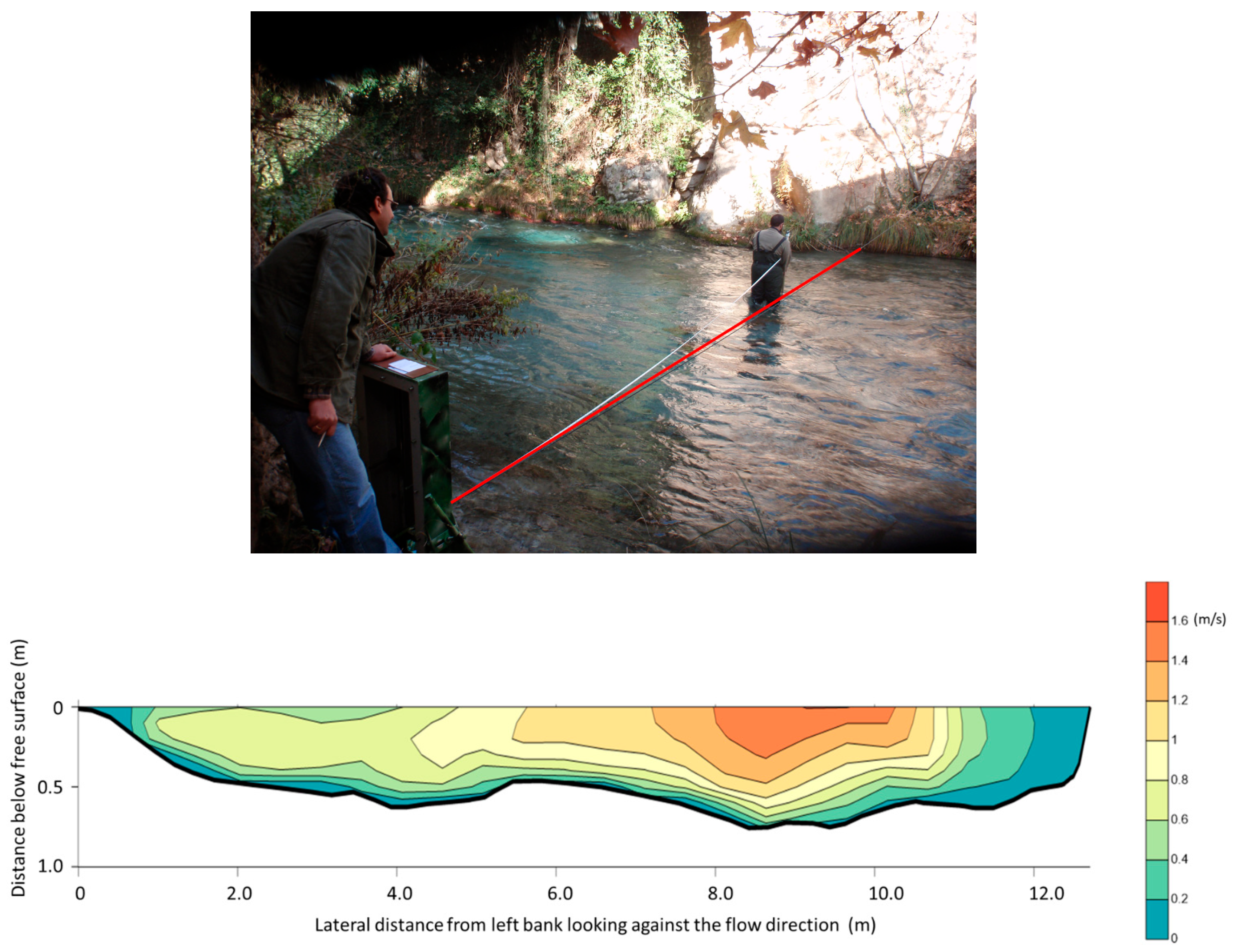
The cross-section of the Loussios River at Atsicholos Bridge is shallow with a depth/width ≈ 1:20 (Figure 4). The bed material for 0 m ≤ x ≤ ~8.5 m is initially coarse sand mixed with gravel, progressively turning into larger pebbles and stones; for ~8.5 m ≤ x ≤ ~11.5 m, large, irregular but smooth rocks form the bed; for x > 11.5, the steep river bank is rough. The goodness of fit of the velocity data from the log-profiles is important information in assessing the reliability of the f_v-predictions. The data from which the contour plot in Figure 4 has been produced are in Supplementary Material A. The discharge at the monitoring cross-section was Q = 5.264 m³/s [11].

Figure 4. Loussios River monitoring station at Atsicholos Bridge: upper panel—measuring cross-section (red line); lower panel—contours of the velocity field (display exaggerated 2H:1V). Reproduced with permission from [11] lower panel).

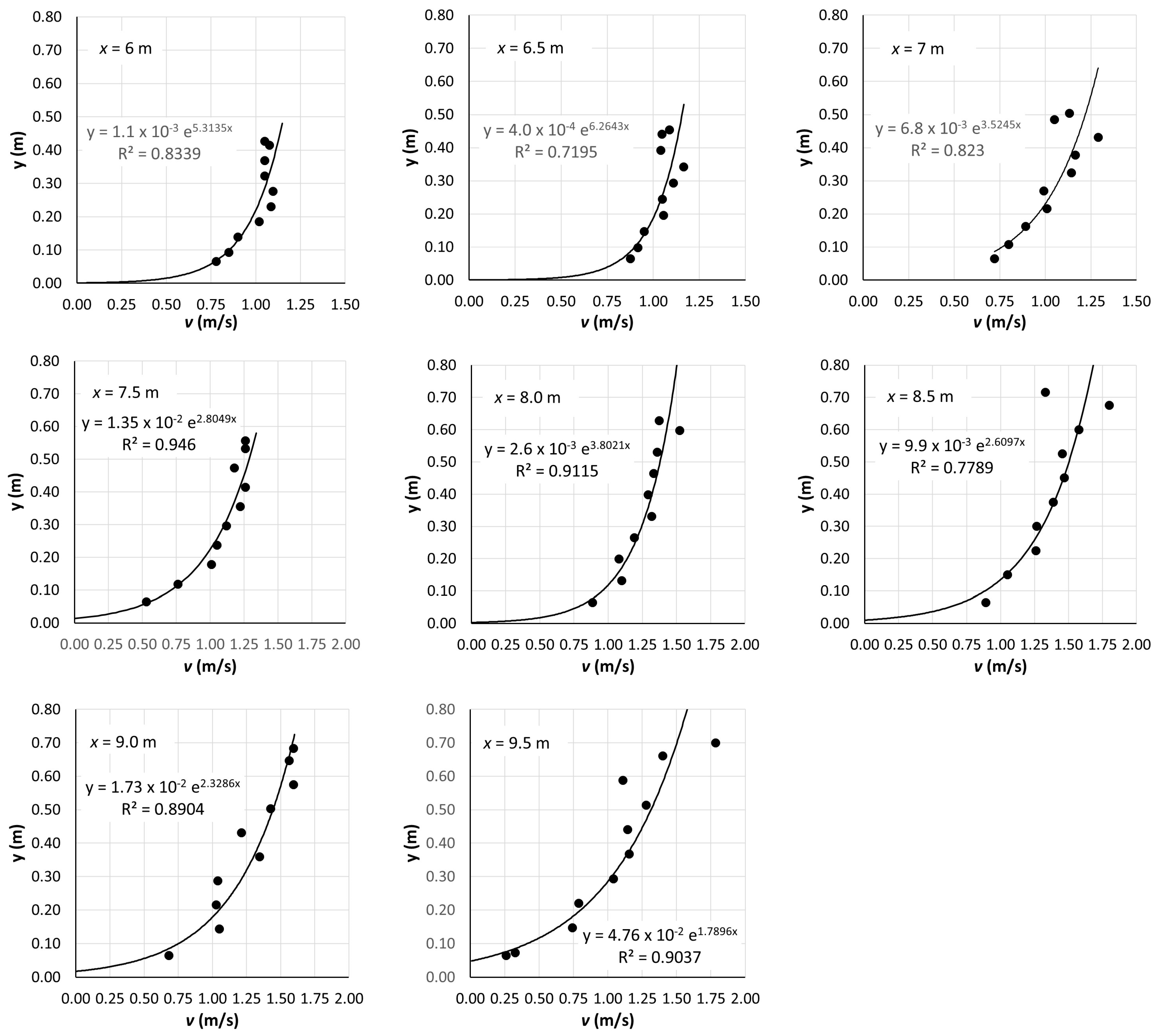
Up to approximately x = 5.5 m, the velocity profiles are not logarithmic (strong dip and r² < 0.5, except at x = 5 m where r² ≈ 0.74). A major reason for this is the influence of the left bank (looking upstream), while the mild hump at 5 m ≤ x ≤ 6.5 m may also cause deviations from the logarithmic law. The deceleration of the flow due to the proximity of the right bank is prominent for x ≥ 11 m. In the range ~6 m ≤ x ≤ ~11 m, all velocity profiles fit the logarithmic model with r² > ~0.7; however, on the verticals at x = 10, 10.5 and 11 m (as at x = 5 m), the profile-fit may be acceptable statistically: 0.7 ≤ r² ≤ 0.81, rather than hydraulically, i.e., conforming visually well to the logarithmic form. This leaves the span 6 m ≤ x ≤ 9.5 m for testing the concept, where the logarithmic model fits the data shown in Figure 5 with 0.72 ≤ r² ≤ 0.95 (average r² ≈ 0.85). Over this span, the bed consists, near the middle of the cross-section, of smooth pebbles of a gradually increasing size of ~5 cm long by ~1.5 cm thick to ~6 cm long by ~3 cm thick, with a rough patch of about x = 7.5 m of irregularly lying ~5–7 cm large stones in a gravely bed, and in the deepest part, x > 8.0 m, of irregularly lying but fairly smooth rocks, ~20 cm long by ~10 cm thick. Despite the smooth surface of many individual roughness elements for x ≥ 7.0 m, the macroscopic bed geometry of this shallow streamflow is fairly rough (submergence h/k < 10).

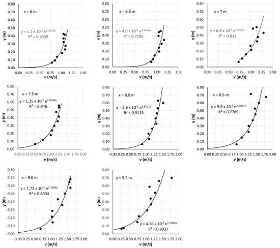
Figure 5. Measured velocities on the verticals x = 6 to 9.5 m in the monitoring cross-section at Atsicholos Bridge over the Loussios River and fitted logarithmic profiles; velocity (m/s) is given on the horizontal axis and distance from bed (m) on the vertical axis.

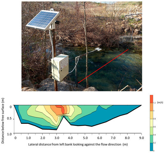
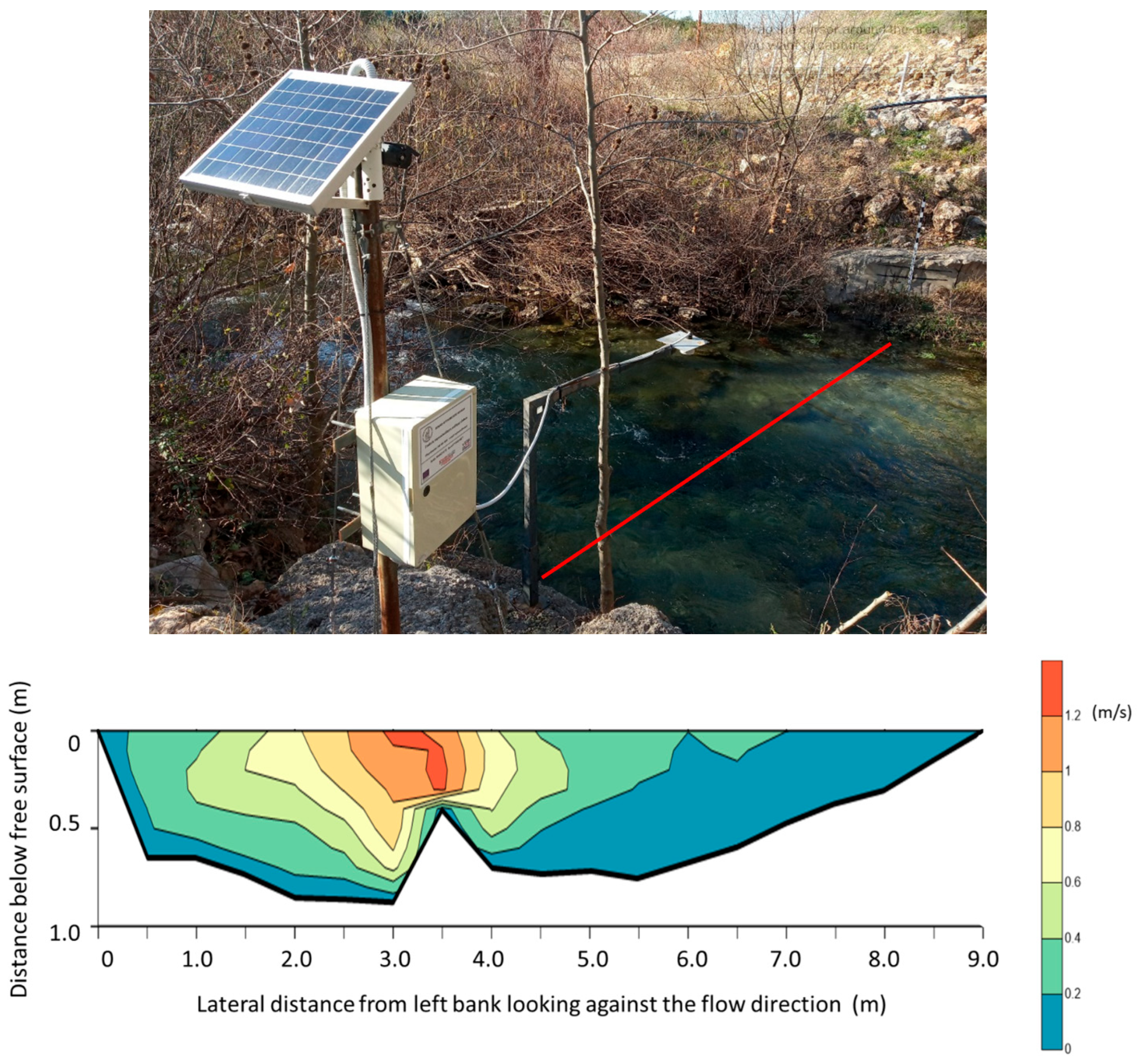
In the monitoring cross-section of the Evrotas River (Figure 6), a pronounced unevenness at x = 3.5 m creates two distinct sub-regions. The bed is largely rough—20 cm rough stones and 2–3 cm gravel over 0 m < x ≤ ~5.5 m—but less rough about the hump, as the larger stones lie on the flat part of the bed: over ~5.5 m ≤ x ≤ 9 m, rocks and gravel first and then sand and mud. The irregular geometry and diverse bed material promote the formation of very different velocity profiles.

Figure 6. Evrotas River monitoring station near the village of Karavas, Laconia: upper panel—location of the station and measuring cross-section (red line); lower panel—contours of the velocity field at the monitoring station (display is exaggerated 2V:1H dimension). Reproduced with permission from [11] (lower panel).

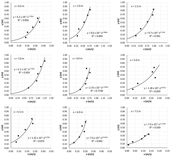
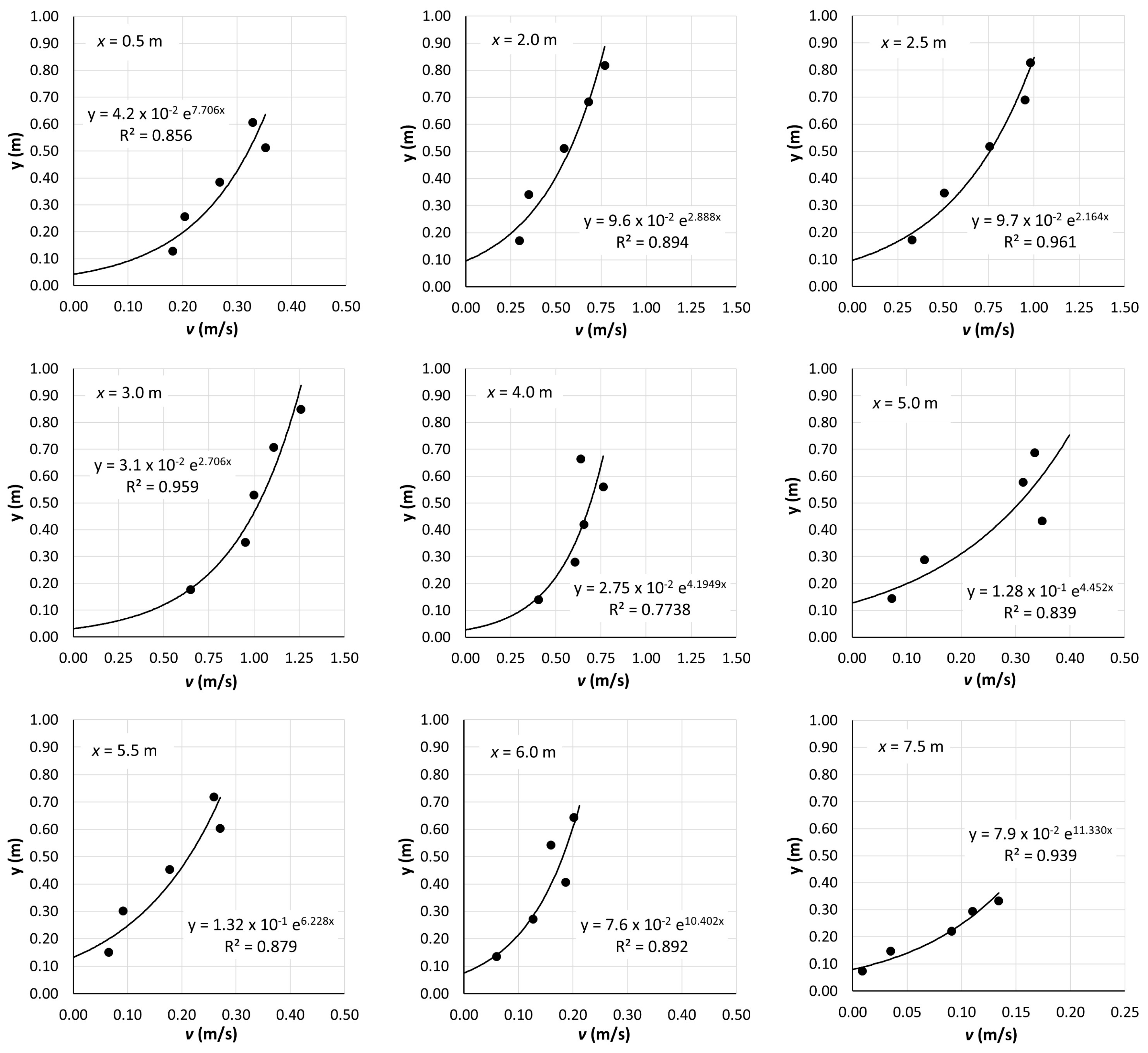
Figure 6 presents the velocity field in contour form; see Supplementary Material A for the data from the monitoring station of the Evrotas River near the village of Karavas. The discharge at the monitoring cross-section was Q = 1.995 m³/s [11]. Logarithmic profiles were fitted to the data on the verticals at x = 0.5, 2.0, 2.5, 3.0, 4.0, 5.0, 5.5, 6.0 and 7.5 m, from the left bank looking downstream (Figure 7). As noted, these profiles vary considerably across the stream, also indicated by markedly varying exponents and y_o-values of the regression curves. Velocities are expectedly higher in the deeper subsection, 1.5 m ≤ x < ~3.0 m; those in the shallower subsection, ~4.0 m < x ≤ 8.0 m, are noticeably lower (also, and especially close to the banks, x ≤ 1.0 m and x ≥ 8.0 m). Note that the velocity scale (horizontal axis) is ~1 m/s in the graphs for 2.0 m ≤ x ≤ 4.0 m but merely ~0.3 m/s in the other graphs, yet the depths differ only by a factor of 1.5–2. The uniformly high velocities of ~1.2 m/s at the hump at x = 3.5 m, h = 0.407 m, are expectedly regressed poorly (r² ≈ 0.32, not graphed). The poor fit at x = 4.0 m (r² = 0.77) is reasonably explained by the proximity to the hump and by the abrupt flow deceleration in the shallower subsection. The logarithmic law fits the data next to the bank, x = 0.5 m, surprisingly well (r² = 0.856), considering that the ‘infinitely wide channel, 2D flow’ assumption is poorly met, yet the log-profile fails to fit the data well at x = 1.0 m, r² ≈ 0.3. Near the opposite bank (x ≥ 6.0 m, approximately), the inclined boundary (1V:5H) slows down the shallow flow markedly (max v ≈ 0.2 m/s). In general, the logarithmic law appears to fit several profiles over ~0.5 m ≤ x ≤ ~7.5 m well enough to test the proposed concept (r² > 0.77).

Figure 7. Velocities measured at 9 verticals in the monitoring cross-section of the Evrotas River, with fitted logarithmic profiles; velocity is on the horizontal axis and distance from bed on the vertical axis.

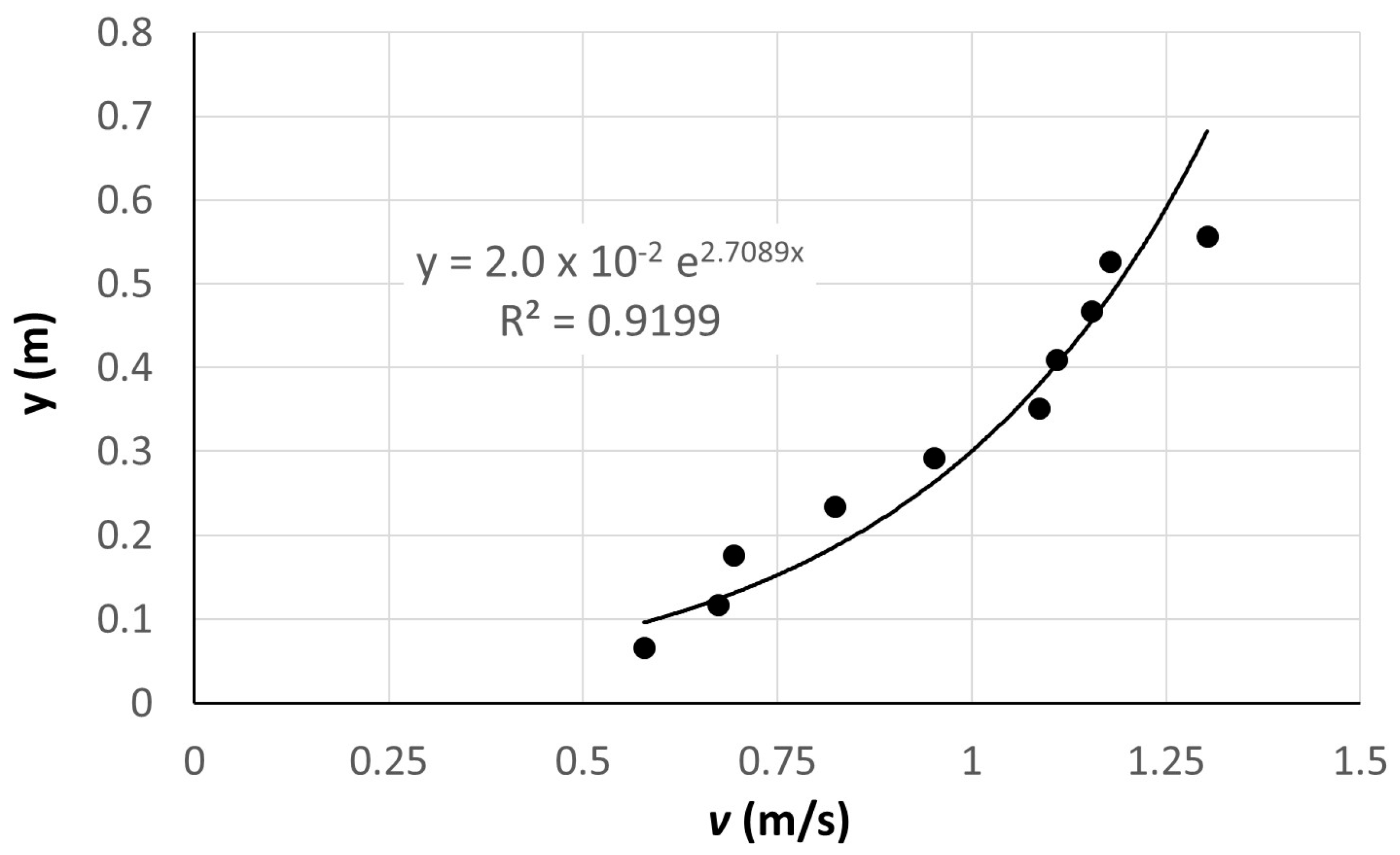
Alagonia Creek is a small tributary of the Upper Nedon River that originates on Mount Taygetos and discharges into the Messinian Bay, traversing the city of Kalamata, SW Peloponnese. During the sampling, the maximum depth in the cross-section near the Rentifi Mill was h = 0.584 m, and the surface width was b ≈ 2.95 m. Detailed sampling was carried out in intervals of ~10% depth, at verticals 0.2 to 0.5 m apart, plus at 0.2 m from the steep left bank and at 0.75 m from the intersection of the free surface with the sloping right bank (looking downstream). The data measured on the vertical with the maximum depth, h = 0.584 m, at the lateral distance x = 0.9 m from the left bank, are graphed in Figure 8, along with the fitted logarithmic profile (r² ≈ 0.92). Over the first meter from the left bank, the bed is armored with rough stones/rocks of 5–10 cm size.

Figure 8. Velocities measured at the x = 0.7 m vertical in the Rentifi Mill cross-section of Alagonia Creek and fitted log-profile; velocity is on the horizontal axis and distance from bed on the vertical axis.

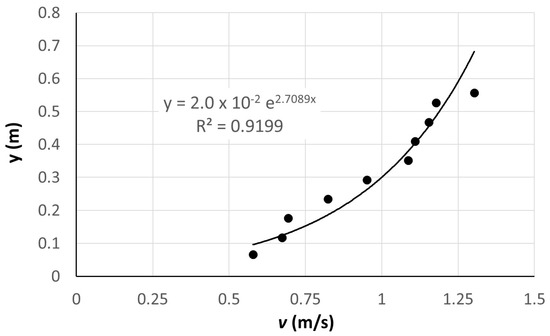
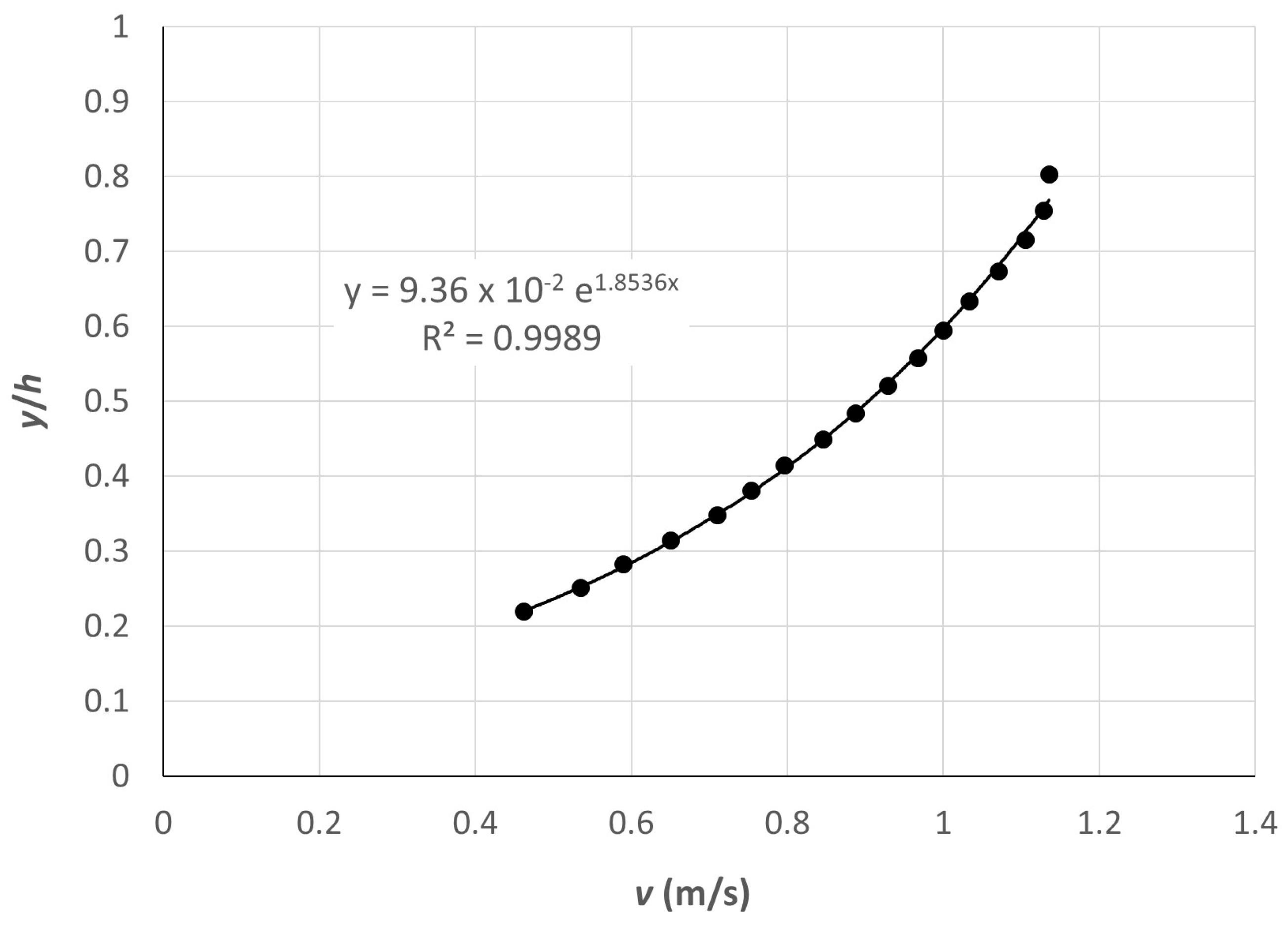
Finally, we sourced data for the Venoge River (canton Vaud, Switzerland) from [35]. The measuring cross-section is located in a straight reach, has a mean depth of h = 0.21 m, a width of b = 6.30 m, a bed slope of S_o = 0.33%, and D₅₀ = 40 mm. Detailed data were collected with an Acoustic Doppler Velocity Profiler (ADVP) over one half of the cross-section; a depth-scaled profile, <v> (0 < y/h ≤ ~0.85), was generated from the data ensemble—figure 8a in [35] (note the dip at y/h ≈ 0.85), reproduced here as Figure 9—excluding the top point and points with y/h < ~0.2. The ADVP’s blanking distance did not allow for measurement in the top ~15% of the water column, and the surface velocity was not measured, so the f_v-ratio cannot be estimated from the data directly (but see the Discussion Section below). However, we can test the friction velocity, length, and von Karman’s κ derived from the data against those equivalent parameters of the double-averaged logarithmic profile, as parameterized in [35].

Figure 9. Ensemble logarithmic velocity profile for Venoge River, adapted from [35].

6. Discussion

Loussios River. The f_v-ratio computed with the friction length determined from the observed data varies considerably across the stream [0.704, 0.860] (Table 2), with values of f_v < 0.8 corresponding to the region with h/y_o < 100; hence, the default ratio in hydrometry, f_v = 0.86, is a poor estimate for these profiles. The results differ when f_v is computed based on the inspected roughness, k, via (a) Equation (11) and y_o = ck; c(h/D₈₄) via Equation (12); and (b) Equation (5) with y_o = k/30. The former better approximates the f_v-ratios from the observed friction length. These two sets of predicted f_v-ratios differ substantially in the two areas of the cross-section where k = 0.1 m and h/k ≤ ~10, in which the results of Equation (11) are close (within ±~6%) to those of Equation (5), with y_o estimated from the observed profiles, while those of Equation (5) with Nikuradze’s friction length, y_o = k/30, are higher by ~9.6%, on average. It follows, therefore, that the amended friction-length formula—y_o = ck and c = 8.61(h/D₈₄)^−1.821 (Equations (10) and (12))—could be applied to shallow streams with a rough bed, for example, h/k ≤ 30. Also, all f_v values at x = 6.5 m, despite their agreement, seem less reliable due to the mediocre fit of the log-profile, r² ≈ 0.72, which can be attributed to the presence of a maximum-velocity dip to y ≈ 0.35 m, y/h ≈ 0.7.

Table 2. Loussios River: f_v = V/$v$_surf from Equation (5) based on (a) observed profiles and (b) Nikuradze’s y_o = k/30 and from Equation (11) based on estimated bed roughness and y_o = ck, c ≈ 8.61(h/D₈₄)^−1.821 ≥ 1/30.

Location	Depth	From Velocity Data			From Bed Inspection					With Nikuradze’s Formula
x [m]	h [m]	yo [m]	h/yo	fv Equation (5)	k [m]	h/k	yo = ck [m]	h/yo	fv Equation (11)	yo = k/30 [m]	h/yo	fv Equation (5)
6.0	0.460	0.0011	418	0.837	0.015	30.7	0.0003	1764	0.867	0.0005	920	0.855
6.5	0.489	0.0004	12225	0.860	0.015	32.6	0.0002	2096	0.870	0.0005	978	0.856
7.0	0.539	0.0068	79.3	0.784	0.03	18.0	0.0014	390	0.835	0.0010	540	0.843
7.5	0.591	0.0135	43.8	0.759	0.05	11.8	0.0049	120	0.799	0.0017	355	0.8325
8.0	0.664	0.0026	2555	0.824	0.03	22.1	0.0009	703	0.849	0.0010	664	0.848
8.5	0.751	0.0099	75.9	0.782	0.1	7.5	0.0225	33.3	0.746	0.0033	225	0.820
9.0	0.719	0.0173	41.6	0.756	0.1	7.2	0.0244	29.5	0.740	0.0033	216	0.819
9.5	0.735	0.0476	15.4	0.704	0.1	7.4	0.0234	31.4	0.743	0.0033	2205	0.819

Evrotas River. The data listed in Table 3 show that the f_v-ratios computed with Equation (5) using friction lengths determined from the observed profiles vary markedly [0.623, 0.738]. It is worth noting that all ratios are substantially less than the default f_v = 0.86; this is due to their association with the values of the inverted scaled friction length, h/y_o < 100, well below those suggested in [13] for streams: 10² ≤ h/y_o ≤ 10⁴. The h/y_o-values that are based on the inspected bed roughness are also in a relatively low range [9, 678] because they derive from large roughness elements in this shallow stream, so the amended friction length, y_o = ck, c = 8.61(h/D₈₄)^−1.821 (Equations (10) and (12)), yields fairly low h/y_o values. The range of the resulting f_v-ratios computed with Equation (11) is [0.666, 0.850] (Table 3), +10% on average relative to those obtained with observed friction lengths, but at x = 3, 4, and 6, 7.5 m ratios are overestimated by 10–20%. The corresponding f_v-ratios in Table 3 determined with Nikuradze’s friction length, y_o = k/30, are higher by ~22%, on average [0.802, 0.848], even though the h/y_o-values are relatively low too (128 to 678); therefore, Nikuradze’s formula cannot account adequately for the actual, high-roughness field conditions.

Table 3. Evrotas River: f_v = V/$v$_surf from Equation (5) based on (a) observed profiles and (b) Nikuradze’s y_o = k/30 and from Equation (11) based on estimated bed roughness and y_o = ck, c ≈ 8.61(h/D₈₄)^−1.821 ≥ 1/30.

Location	Depth	From Velocity Data			From Bed Inspection					With Nikuradze’s Formula
x [m]	h [m]	yo [m]	h/yo	fv Equation (5)	k [m]	h/k	yo = ck [m]	h/yo	fv Equation (11)	yo = k/30 [m]	h/yo	fv Equation (5)
0.5	0.641	0.042	15.3	0.703	0.15	4.3	0.0750 *	8.5	0.666	0.005	128	0.802
2	0.853	0.096	8.9	0.669	0.15	5.7	0.0750 *	11.4	0.685	0.005	171	0.811
2.5	0.862	0.097	8.9	0.669	0.15	5.7	0.0750 *	15.8	0.686	0.005	172	0.812
3	0.883	0.031	28.5	0.738	0.05	17.7	0.0024	373	0.834	0.00167	530	0.842
4	0.699	0.0275	25.4	0.732	0.05	14	0.0036	193	0.815	0.00167	419	0.837
5	0.722	0.128	5.6	0.637	0.15	4.8	0.0764	9.5	0.673	0.005	144	0.806
5.5	0.754	0.132	5.7	0.638	0.15	5	0.0709	10.6	0.681	0.005	151	0.807
6	0.678	0.076	8.9	0.669	0.03	22.6	0.0009	7455	0.850	0.001	678	0.848
7.5	0.367	0.079	4.6	0.623	0.03	12.2	0.0028	131	0.803	0.001	367	0.833

* Values from inspected k = 0.15 m in 4.3 ≤ h/k ≤ 5.7 are estimated as y_o = ck = 0.075 m with c fixed at c(h/k = 5) = 0.5.

Alagonia Creek. The logarithmic profile fitted to the data (r² ≈ 0.92) (Figure 8) is v(y) ≈ 0.37 ln(y/0.02) = 0.37 ln(50y), so y_o ≈ 0.02 m (and $v_{*}/\kappa$= 0.37, $v_{*}$ ≈ 0.152 m/s for κ = 0.41), which yields as mean velocity is V ≈ 0.88 m/s, and $v$_surf ≈ 1.248 m/s, and thus, f_v ≈ 0.705. Then, with h = 0.584 m, (a) h/y_o = 0.584/0.02 = 29.2, and Equation (5) gives f_v = 0.74; (b) if the roughness is estimated as the mean, <k> = (0.1 m + 0.05 m)/2 = 0.075 m, h/<k> ≈ 7.8. and c ≈ 0.2, Equations (10)–(12) yield f_v ≈ 0.75: f_v ≈ 0.74–0.75 is fair for a rugged headwater stream and much better than the default f_v = 0.86. In contrast, y_o = <k>/30 = 0.0025 gives h/y_o ≈ 232 and f_v ≈ 0.82 (a poorer but still more useful estimate than f_v = 0.86).

Venoge River. We used the ensemble profile with the average granularity of the bed material over the bed (no local variation). Fitting a depth-scaled logarithmic velocity profile, v(y/h) = (v_*/κ)ln[(y/h)/(y_o/h)], to the data ensemble yields v = 0.536 ln[(y/h)/0.0936], r² ≈ 0.999 (Figure 9); given h = 0.21 m [35], y_o ≈ 0.02 m with $v_{*}$ = $\sqrt{gh{S}_{\mathrm{o}}}$ ≈ 0.082 m/s, κ ≈ 0.152. The corresponding results in table 2 of [35] are y_o ≈ 0.066 m, v_* = 0.078 m/s and κ = 0.17. There is thus fair agreement between corresponding values of $v_{*}$ and κ, but not of y_o. However, y_o can be estimated directly as follows. Figure 4 in [35] at D₈₄ ≈ 85 mm yields h/D₈₄ ≈ 2.3. As this submergence value lies outside of the h/D₈₄-range [5,20] used to assign c-values (then fitted by Equation (12)), we extrapolate linearly from the (h/D₈₄, c)–pairs (10, 0.1) and (5, 0.5) to h/D₈₄ = 2.3 and obtain c = 0.716 and the good estimate y_o = 0.061 m (nevertheless, extrapolation beyond the calibration range of Equation (12) warrants caution). The f_v-ratio estimated from the ensemble log-profile, f_v = 0.7367/1.269 ≈ 0.58, and by Equation (5) with y_o(h/D₈₄ = 2.3) = 0.061 m, f_v ≈ 0.61, are just 5% apart and in excellent agreement with the estimate of Greco and Martino ([29], cf. Figure 4)) f_v ≈ 0.6, and all far from f_v = 0.86; (the error relative to the data-derived f_v is (0.86–0.58)/0.58 = 0.48, i.e., a 48% discharge overestimation). For comparison, Equation (9) ([18]), with v_* = 0.082 m/s, κ = 0.152 and v_surf ≈ 1.269 m/s, gives f_v ≈ 0.437 (for v_surf ≈ v(y/h = 0.8) ≈ 1.15 m/s, f_v ≈ 0.665). The wall Reynolds number, R_w ≈ 7000, classifies the flow regime of the Venoge River as hydraulically rough.

7. Conclusions

This work set out to provide guidance to hydrographers in estimating the ratio of mean to surface velocity in rough-bed streams when velocity profile data are absent. Considerations of hydromechanics and assessment of the reported laboratory and field cases support the following conclusions:

• The mean-to-surface-velocity ratio f_v(y_o/h) derived from the Prandtl–von Kármán logarithmic velocity profile with the friction length, y_o, evaluated based on an estimated bed roughness—through inspection or via sieve analysis of the bed material (cf. Venoge River case)—is more reliable than the default f_v = 0.86. This assessment rests on data fitted by log-profiles with r² ≥ 0.72 and holds regardless of whether y_o is described by Equation (2) or by Equations (10) and (12). The dependence of f_v on the depth-scaled friction length enables accounting for cross-sectional variability and better flow estimation after appropriate segmentation.
• Specifically, if the streambed is granular and rough, i.e., consisting of gravels and rocks, and the depth is shallow, giving submergence values ~5 ≤ h/D₈₄ < ~30, comparing f_v-ratios derived from velocity field data against f_v-ratios evaluated with the inspected roughness show that y_o = ck, 0.013 < c ≤ 0.5, k ≈ D₈₄, c ≈ 8.61(h/k)^−1.821, Equations (11) and (12) more closely estimate the field-data-derived f_v-ratios than Nikuradze’s y_o = k/30 with Equation (5). Practically, f_v(y_o/h) with y_o = ck, c ≈ 8.61(h/k)^−1.821, Equation (12), holds within ~|10|% error, on average (range 3–20%), for granular stream boundaries down to the start of the intermediate roughness scale of [33] and is robust against misestimating roughness; y_o = k/30 (Equation (2)) is suitable for shallow and large streams with smooth beds, for example, h/k ≥ 30, giving f_v ≥ 0.86.
• The classification of resistance in boundary-layer flow by the wall Reynolds number, R_w = $v_{*}$k/ν, for the two extreme test cases, Yeh’s laboratory experiment, R_w ≈ 4, and the Venoge River, R_w ≈ 7000, suggests that the proposed formulation describes flow from the start of the transition zone, R_w = 4, to well in the hydraulically rough regime, R_w > 100 [30].
• The proposed method merits consideration in hydrometry, as the present study assessed the suitability of the friction-length ansatz, y_o/k = c(h/k) ≥ 1/30, c ≈ 8.61(h/k)^−1.821 (Equation (12)), in challenging streamflow cases over a fairly wide range of relative roughness. With additional validation, this concept may also prove useful for h/k < 5, as shown by extrapolation in the case of the Venoge River. In the intermediate roughness scale of Bathurst et al. (1981) [33], fitting a logarithmic velocity profile to the data may require a von Kármán constant smaller than κ = 0.4 (cf. [35]), but care is due, as ‘κ operates in an inverse manner to $v$_*, an error in $v$_* can be concealed by adjusting κ and vice versa’ [42].

Suggestions for further research: The mean-to-surface-velocity ratio derived from the Prandtl–von Kármán logarithmic velocity law, by definition, cannot account for the variable macro-geometry of a natural stream’s cross-section, as the log-law assumes an infinitely wide channel (an assumption shared by current hydrometric practice). The influence of the macro-geometry could be studied initially by conducting laboratory experiments in rectangular flumes of various widths, but at the same depth (variable h/b) and with the same granular roughness (constant relative roughness).

References

- Tauro, F.; Selker, J.; van de Giesen, N.; Abrate, T.; Uijlenhoet, R.; Porfiri, M.; Manfreda, S.; Caylor, K.; Moramarco, T.; Benveniste, J.; et al. Measurements and Observations in the XXI century (MOXXI): Innovation and multidisciplinarity to sense the hydrological cycle. Hydrol. Sci. J. 2018, 63, 169–196. [Google Scholar] [CrossRef] [Scilit]
- Bandini, F.; Lüthi, B.; Peña-Haro, S.; Borst, C.; Liu, J.; Karagkiolidou, S.; Hu, X.; Lemaire, G.G.; Bjerg, P.L.; Bauer-Gottwein, P. A drone-borne method to jointly estimate discharge and Manning’s roughness of natural streams. Water Resour. Res. 2020, 57, e2020WR028266. [Google Scholar] [CrossRef] [Scilit]
- World Meteorological Organization. Manual on Stream Gauging; Vol. I Fieldwork, WMO-No. 1044; WMO: Geneva, Switzerland, 2010. [Google Scholar]
- Costa, J.E.; Cheng, R.T.; Haeni, F.P.; Melcher, N.; Spicer, K.R.; Hayes, E.; Plant, W.; Hayes, K.; Teague, C.; Barrick, D. Use of radars to monitor stream discharge by noncontact methods. Water Resour. Res. 2006, 42, W07422. [Google Scholar] [CrossRef] [Scilit]
- Muste, M.; Fujita, I.; Hauet, A. Large-scale particle image velocimetry for measurements in riverine environments. Water Resour. Res. 2008, 44, W00D19. [Google Scholar] [CrossRef] [Scilit]
- Fujita, I.; Notoya, Y.; Tani, K.; Tateguchi, S. Efficient and accurate estimation of water surface velocity in STIV. Environ. Fluid Mech. 2019, 19, 1363–1378. [Google Scholar] [CrossRef] [Scilit]
- LeGrand, M.; Luce, J.; Metcalfe, R.; Buttle, J. Development of an inexpensive automated streamflow monitoring system. Hydrol. Process. 2020, 34, 3021–3023. [Google Scholar] [CrossRef] [Scilit]
- Rozos, E.; Dimitriadis, P.; Mazi, K.; Lykoudis, S.; Koussis, A. On the uncertainty of the image velocimetry method parameters. Hydrology 2020, 7, 65. [Google Scholar] [CrossRef] [Scilit]
- Welber, M.; Le Coz, J.; Laronne, J.; Zolezzi, G.; Zamler, D.; Dramais, G.; Hauet, A.; Salvaro, M. Field assessment of noncontact stream gauging using portable surface velocity radars (SVR). Water Resour. Res. 2016, 52, 1108–1126. [Google Scholar] [CrossRef] [Scilit]
- US Geological Survey. Measurement and Computation of Streamflow in Measurement and Computation of Streamflow; US Geological Survey: Reston, VA, USA, 1982; Volume 1, p. 137. Available online: https://www.semanticscholar.org/paper/Measurement-and-computation-of-streamflow%3A-Volume-Rantz/35825c14729f8740803d953e63f4753c11b16841 (accessed on 11 February 2026).
- Koussis, A.D.; Dimitriadis, P.; Lykoudis, S.; Kappos, N.; Katsanos, D.; Koletsis, I.; Psiloglou, B.; Rozos, E.; Mazi, K. Discharge estimation from surface-velocity observations by a maximum-entropy based method. Hydrol. Sci. J. 2022, 67, 451–461. [Google Scholar] [CrossRef] [Scilit]
- ISO 748:2007; Hydrometry—Measurement of Liquid Flow in Open Channels Using Current-Meters or Floats. ISO: Geneva, Switzerland, 2007. Available online: https://www.iso.org/standard/37573.html (accessed on 17 January 2024).
- Le Coz, J.; Hauet, A.; Pierrefeu, G.; Dramais, G.; Camenen, B. Performance of image-based velocimetry (LSPIV) applied to flash-flood discharge measurements in Mediterranean rivers. J. Hydrol. 2010, 394, 42–52. [Google Scholar] [CrossRef] [Scilit]
- Hauet, A.; Morlot, T.; Daubagnan, L. Velocity profile and depth-averaged to surface velocity in natural streams: A review over a large sample of rivers. In Proceedings of the E3S Web of Conferences, River Flow, Lyon-Villeurbanne, France, 5–8 September 2018. [Google Scholar] [CrossRef] [Scilit]
- Bjerklie, D.M.; Fulton, J.W.; Dingman, S.L.; Canova, M.G.; Minear, J.T.; Moramarco, T. Fundamental hydraulics of cross sections in natural rivers: Preliminary analysis of a large data set of acoustic Doppler flow measurements. Water Resour. Res. 2020, 56, e2019WR025986. [Google Scholar] [CrossRef] [Scilit]
- Moramarco, T.; Dingman, S.L. On the theoretical velocity distribution and flow resistance in natural channels. J. Hydrol. 2017, 555, 777–785. [Google Scholar] [CrossRef] [Scilit]
- Song, S.; Schmalz, B.; Fohrer, N. Improved structure of vertical flow velocity distribution in natural rivers based on mean vertical profile velocity and relative water depth. Hydrol. Res. 2018, 49, 878–892. [Google Scholar] [CrossRef] [Scilit]
- Biggs, H.; Smart, G.; Holwerda, N.; Doyle, M.; McDonald, M.; Ede, M. River Discharge from Surface Velocity Measurements—A Field Guide for Selecting Alpha; Envirolink Advice Report; ResearchGate: Christchurch, New Zealand, 2021. [Google Scholar]
- Biggs, H.; Smart, G.; Doyle, M.; Eickelberg, N.; Aberle, J.; Randall, M.; Detert, M. Surface Velocity to Depth-Averaged Velocity—A Review of Methods to Estimate Alpha and Remaining Challenges. Water 2023, 15, 3711. [Google Scholar] [CrossRef] [Scilit]
- Schlichting, H. Grenzschicht-Τheorie; G. Braun Verlag: Karlsruhe, Germany, 1965. [Google Scholar]
- Daily, J.W.; Harleman, D.R.F. Fluid Dynamics; Addison-Wesley Publishing Co.: Reading, MA, USA, 1973. [Google Scholar]
- Schröder, R.C.M. Technische Hydraulik; Springer: Berlin/Heidelberg, Germany, 1994. [Google Scholar]
- Dingman, S.L. Comment on “Probabilistic approach to modeling of velocity distributions in fluid flows” by C.-L. Chiu and S.-M. Hsu, Journal of Hydrology 316:28–42. J. Hydrol. 2007, 335, 419–428. [Google Scholar]
- Cheng, N.-S. Power-law index for velocity profiles in open channel flows. Adv. Water Resour. 2007, 30, 1775–1784. [Google Scholar] [CrossRef] [Scilit]
- Tennekes, H.; Lumley, J.L. A First Course in Turbulence; MIT Press: Cambridge, MA, USA, 1972. [Google Scholar]
- Southhard, J. Introduction to Fluid Motion and Sediment Transport; MIT Press: Cambridge, MA, USA, 2022. [Google Scholar]
- Nikuradse, J. Stroemungsgesetze in Rauhen Rohren; Forschung auf dem Gebiete des Ingenieurwesens, Heft 361; Verein Deutscher Ingenieure: Düsseldorf, Germany, 1933. [Google Scholar]
- Chow, V.T. Open-channel Hydraulics; McGraw-Hill: Columbus, OH, USA, 1959. [Google Scholar]
- Greco, M.; Martino, G. 1-D versus 2-D entropy velocity law for water discharge assessment in a rough ditch. Entropy 2018, 20, 638. [Google Scholar] [CrossRef] [Scilit]
- Henderson, F.M. Open Channel Flow; Chapter 10; Macmillan Publishing Co.: New York, NY, USA, 1966. [Google Scholar]
- Ferguson, R. Flow resistance equations for gravel- and boulder-bed streams. Water Resour. Res. 2007, 43, W05427. [Google Scholar] [CrossRef] [Scilit]
- Rickenmann, D.; Recking, A. Evaluation of flow resistance in gravel-bed rivers through a large field data set. Water Resour. Res. 2011, 47, W07538. [Google Scholar] [CrossRef] [Scilit]
- Bathurst, J.C.; Li, R.M.; Simons, D.B. Resistance equation for large-scale roughness. J. Hydraul. Eng. 1981, 107, 1593–1613. [Google Scholar] [CrossRef] [Scilit]
- Keulegan, G.H. Laws of Turbulent Flow in Open Channels; National Bureau of Standards: Gaithersburg, MD, USA, 1938; Volume 21, pp. 707–741. [Google Scholar]
- Franca, M.J.; Ferreira, R.M.L.; Lemmin, U. Parameterization of the logarithmic layer of double-averaged streamwise velocity profiles in gravel-bed river flows. Adv. Water Res. 2008, 31, 915–925. [Google Scholar] [CrossRef] [Scilit]
- Haws, B.B. Ability of ADV Measurements to Detect Turbulence Differences Between Angular and Rounded Gravel Beds of Intermediate-Roughness Scale. Master’s Thesis, Brigham Young University, Provo, UT, USA, 2008. [Google Scholar]
- Monzavi, M.T. Widerstandsgesetz Auf Statistischer Basis Für Extreme und Natürliche Rauhigkeiten in Druckrohren; Tech. Ber. 8; Institut für Hydraulik & Hydrologie, T.H. Darmstadt: Darmstadt, Germany, 1972. [Google Scholar]
- Nassrullah, S.; Stubbs, A.; Stoesser, T.; Wilson, C.A.M.E. The validation of the logarithmic velocity profiles above rough-bed flows. In Proceedings of the 38th IAHR World Congress, Panama City, Panama, 1–6 September 2019. [Google Scholar] [CrossRef] [Scilit]
- Yen, B.C. Characteristics of Subcritical Flow in a Meandering Channel. Ph.D. Thesis, The University of Iowa, Iowa City, IA, USA, 1965. [Google Scholar]
- Mazi, K.; Koussis, A.D.; Lykoudis, S.; Psiloglou, B.E.; Vitantzakis, G.; Kappos, N.; Katsanos, D.; Rozos, E.; Koletsis, I.; Kopania, T. Establishing and operating (Pilot Phase) a telemetric streamflow monitoring network in Greece. Hydrology 2023, 10, 19. [Google Scholar] [CrossRef] [Scilit]
- Mamassis, N.; Mazi, K.; Dimitriou, E.; Kalogeras, D.; Malamos, N.; Lykoudis, S.; Koukouvinos, A.; Tsirogiannis, I.; Papageorgaki, I.; Panagopoulos, Y.; et al. OpenHi.net: A Synergistically Built, National-Scale Infrastructure for Monitoring the Surface Waters of Greece. Water 2021, 13, 2779. [Google Scholar] [CrossRef] [Scilit]
- Smart, G. A base for the log law and von Karman’s constant problem. J. Hydraul. Res. 2022, 60, 935–943. [Google Scholar] [CrossRef] [Scilit]
- Le Coz, J.; Pierrefeu, G.; Paquier, A. Evaluation of river discharges monitored by a fixed side-looking Doppler profiler. Water Resour. Res. 2008, 44, W00D09. [Google Scholar] [CrossRef] [Scilit]
Disclaimer/Publisher’s Note: The statements, opinions and data contained in all publications are solely those of the individual author(s) and contributor(s) and not of MDPI and/or the editor(s). MDPI and/or the editor(s) disclaim responsibility for any injury to people or property resulting from any ideas, methods, instructions or products referred to in the content. |
© 2026 by the authors. Licensee MDPI, Basel, Switzerland. This article is an open access article distributed under the terms and conditions of the Creative Commons Attribution (CC BY) license.