Reconstructing Shallow River Bathymetry Through Sequence-Based Modeling Approach

Abstract

Hydrological monitoring is crucial for protecting aquatic ecosystems, especially downstream of hydropower plants where water levels can change suddenly and cause the degradation of instream habitats. There are lot of traditional methods used to monitor water levels and river bathymetry, but most of them rely on in situ measurements. Drone-based remote sensing has received more attention in recent years, with the data in turn processed using CNNs. In this paper, we propose a new sequence-based method that uses multiple frames to expand the available context and compare it to already existing methods, such as Lyzenga, Stumpf, CNN, and SfM. The best performing models within this study end up being SfM and CNN, with the former being more accurate on rivers with clean riverbeds and the latter being the most consistent. The sequence-based model shows promise, and even outperforms CNN, in terms of MAE, on rivers where the same location across multiple views is mapped, achieving the most accurate results across different images. This shows that utilizing multiple views to increase the available context can improve the accuracy of riverine depth estimation based on multispectral visual information.

1. Introduction

Hydrological monitoring plays a critical role in understanding and protecting aquatic ecosystems. This need is especially pronounced in river systems where water levels fluctuate in response to human activities, such as hydropower operations. By rapidly increasing or decreasing discharge to meet energy demands, hydropower plants can induce substantial and recurrent changes in river stage. Over time, these fluctuations may lower overall water levels downstream, degrading habitat quality and threatening the stability of local freshwater ecosystems. Continuous monitoring of river water depth—known as bathymetry—is therefore essential for assessing these impacts and informing sustainable water-resource management.

Traditional bathymetric surveys rely on in situ measurements using specialized equipment, which provide high accuracy but are labor-intensive, costly, and often impractical for frequent or large-scale monitoring [1]. Other techniques, such as sonar-based systems [2], can improve efficiency but their use is limited in very shallow rivers, where signal performance degrades; therefore, they are generally used for deeper bodies of water, such as lakes and coastlines [1]. For more shallow waters, the use of Acoustic Doppler Current Profilers (ADCPs) has been proven to create accurate depth measurements; however, they are still not suitable for very shallow rivers [3]. With the advent and rapid advancement of satellite remote sensing, however, new opportunities have emerged for scalable, timely, and non-intrusive bathymetric mapping [4,5,6,7]. As a result, satellite-based bathymetry has become an increasingly active and promising area of research for monitoring river environments, but it is limited by the coarse resolution of satellite imagery [5,8].

In recent years, advances in unmanned aerial vehicle (UAV) technology have further increased interest in using drone-based remote sensing for river bathymetry [9,10]. UAV imagery offers higher spatial resolution and greater flexibility than satellite platforms, and numerous studies have demonstrated that drone-derived measurements can be more accurate for estimating water depth, particularly in shallow or narrow river systems. The use of multispectral sensors mounted on UAVs has shown even greater potential [11], as the additional spectral bands provide richer information on light reflectance from the riverbed, thereby improving depth retrieval models [12,13,14]. Traditional methods for bathymetry from optical data often involve creating a regression model that estimates the water depth based on light reflectance [15,16]. Another popular method that has been proven to be successful for water depth estimation is the use of photogrammetry algorithms, such as Structure-from-Motion [9,17], also known as SfM. The idea behind these methods is to use a set of river images to recreate a 3D representation of said river and calculate its depth in that way [9,18]. Finally, as various machine learning algorithms continue to improve, their use has also been tested and found to be successful for bathometry of various water bodies [4,7,12,19]. Since these methods use optical images to estimate river depth, convolutional neural networks have proven to be particularly successful in this task [11,14,20,21].

A fundamental limitation of optical remote sensing remains light penetration in water, which decreases rapidly with depth due to absorption and scattering. As a result, visual and multispectral methods become ineffective beyond a certain depth threshold, constraining the applicability of UAV-based bathymetry in deeper river sections [22]. In addition, different multispectral bands have different maximum depths that they can penetrate. Among these, the green and near infrared, also known as NIR, bands generally perform the best for accurate depth estimation [19]. Another challenge with visual river bathymetry is the diversity of sediment types in the riverbed, which makes it more difficult to correctly reconstruct the riverbed and calculate the potential depth of a body of water [23,24].

Most existing studies in this field focus on estimating water depth in comparatively deep aquatic environments, such as coastlines, lakes, and large river systems [2,24,25,26,27,28]. By contrast, far fewer investigations address shallow river bathymetry [29], particularly within the Eastern European region [18,30], where the hydrological dynamics and environmental pressures may differ substantially from those of well-studied areas. This paper specifically examines shallow river bathymetry using multispectral imagery acquired by UAVs. Its primary objective is to compare a range of depth-estimation techniques applied to UAV-based multispectral data. Furthermore, the study explores the potential of artificial intelligence (AI) methods to enhance the accuracy and robustness of depth retrieval in shallow river environments, comparing the results against established baselines derived from traditional physics-based depth estimation models. Finally, most existing studies use a single context to estimate the depth of a single region of a body of water. In this study, we aim to utilize multi-view, multi-temporal data from multiple rivers, which would increase the context provided for depth estimation methods and therefore improve the accuracy of such methods.

2. Materials and Methods

This section describes the materials and methods used in this study, including the data acquisition procedures and data sources, processing workflows, and techniques applied for river depth estimation. The methodology is structured to ensure reproducibility and consistency across all stages of the analysis.

2.1. Methodology

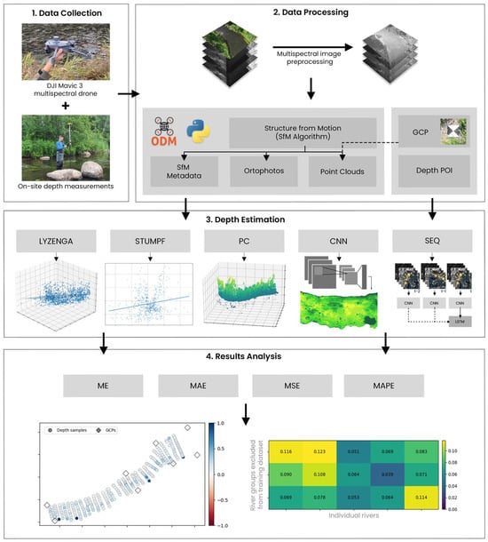
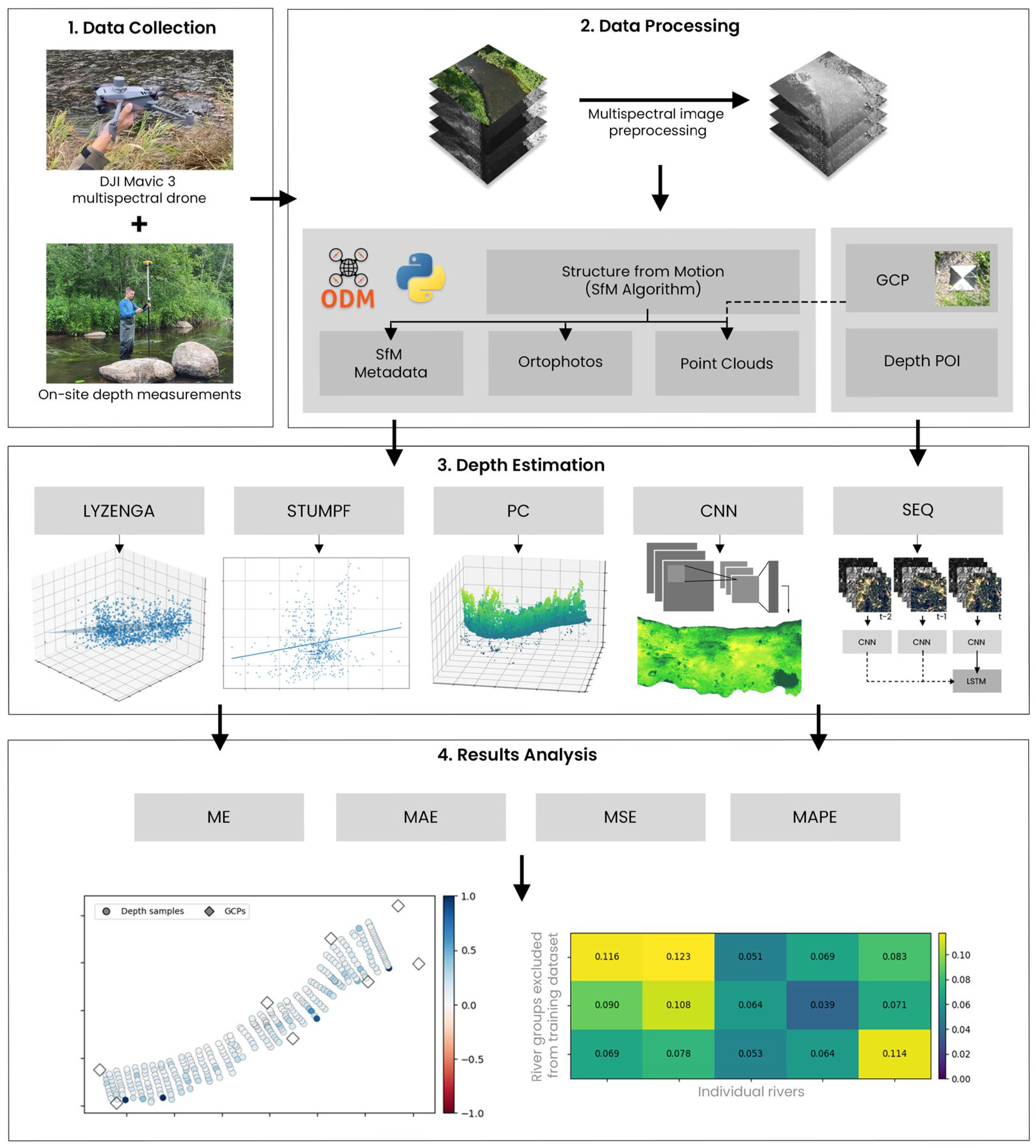
The workflow in this study is organized into four main components, integrating data collection, data processing, river depth estimation and analysis of the results. The overall structure of the workflow is illustrated in Figure 1, and each component is described in the following sections.

Figure 1. The workflow of this study.

The first part involved data collection and consisted of acquiring in situ measurements of the selected river reaches. In addition, RGB and multispectral imagery was collected using an UAV, which was required for the subsequent stages of this study. The second part was data processing, which primarily involved preprocessing the acquired imagery for subsequent application of the SfM algorithm. The resulting outputs were then further processed to ensure their suitability for use in depth estimation. The third part comprised depth estimation, in which various selected techniques were applied to generate depth heatmaps for specific river segments. Finally, the last stage focused on results analysis, where the accuracy of different depth estimation methods used to generate the depth heatmaps was calculated and methods were compared by applying cross-validation techniques to evaluate their ability to generalize across different river scenes.

2.2. Data Collection

The used dataset consisted of images collected over the stretches of three rivers located in Lithuania. Imagery data was collected using a DJI Mavic 3 Multispectral drone (Da-Jiang Innovations, Shenzhen, China) with a 4/3-inch CMOS sensor RGB camera with a resolution of 3840 × 2160 pixels. Each river was captured using four multispectral bands—green (560 nm ± 16 nm), near-infrared (NIR) (840 nm ± 26 nm), red (650 nm ± 16 nm), and red edge (730 nm ± 16 nm)—alongside standard RGB imagery. All captured images included metadata describing the acquisition conditions, including camera position and capture parameters. It is important to note that the RGB images differed in resolution and spatial alignment from the multispectral images, likely due to wind gusts and natural UAV motion during data collection. In addition to the imagery, in situ depth measurements were taken at predefined locations along each river, providing ground-truth georeferenced depth values and corresponding riverbed contours for use in model evaluation. The precise river water surface elevation was also collected and interpolated to digital elevation model (DEM). Finally, precise coordinates and heights for ground control points (GCPs) were also recorded for the use in image geographic calibration. All coordinates and height measurements were obtained using a high-precision GeoMax Zenith 40 GNSS receiver (GeoMax AG, Widnau, Switzerland) and X-PAD Ultimate Survey (version 24.5.1) software. The characteristics of each river can be seen in Table 1.

Table 1. Dataset summary.

River	Date	Point Count	Mean Depth	Minimum Depth	Maximum Depth
Jūra	13 July 2023	305	0.376 ± 0.155	0.090	0.900
	14 September 2023	207	0.439 ± 0.167	0.100	0.920
Mūša	23 September 2024	315	0.381 ± 0.162	0.110	0.850
Šušvė	22 September 2023	238	0.241 ± 0.073	0.080	0.410
	26 June 2024	96	0.256 ± 0.068	0.130	0.440

2.3. Data Processing

The direct application of the SfM algorithm on unprocessed raw multispectral data results in significant data gaps in resulting orthophotos and point clouds. This limitation is especially pronounced in riverbed regions, which are critical for depth estimation. To mitigate this issue, all multispectral were first preprocessed. In this work, this was separated into four parts: image masking, image normalization, SfM and calibration applied to data derived from SfM algorithm. The processes of each method are described in the following subsections.

2.3.1. Water Area Identification

To prepare multispectral imagery for SfM processing, the water area in each image must be identified. Each river image was first filtered using a custom masking procedure. The process began by calculating the Normalized Difference Water Index (NDWI), Normalized Difference Vegetation Index (NDVI), and Normalized Difference Red Edge Index (NDRE). All of these indexes are defined by Equations (1)–(3). Finally, inverted brightness mask, as seen in Equation (4), was calculated to highlight shaded areas from the multispectral images. All of these values were later used to generate an initial mask that highlighted areas covered by various surfaces.

$$NDWI={\displaystyle \frac{G - NIR}{G + NIR}}$$

(1)

$$NDVI={\displaystyle \frac{NIR-R}{NIR+R}}$$

(2)

$$NDRE={\displaystyle \frac{NIR-RE}{NIR+RE}}$$

(3)

$$Brightness={\displaystyle \frac{G+R}{2}}$$

(4)

Here G, R, RE, and NIR correspond to green, red, red edge, and near infrared spectral band reflection values, respectively. An example of these masks along with an example of a multispectral band image can be seen in Figure 2.

Figure 2. Image masking components.

The NDWI index highlighted water surfaces in the multispectral images; however it often failed to correctly identify water in shaded regions. To address this limitation, brightness-based masks were created. The NDWI mask ensured that low-brightness areas identified as land were excluded. A logical OR operation was then applied to combine the NDWI and brightness masks. In some cases, this combined mask failed to correctly identify the contour of the river. This occurred due to vegetated areas that have similar values as water. To solve this, the NDVI and NDRE indexes were used to highlight vegetation in the image. A logical OR operation was once again performed between these masks, and the result was inverted to obtain a mask that excluded all vegetation from the image. Finally, a logical AND operation was performed between the water and the inverted vegetation masks to obtain the final river masks.

2.3.2. Image Normalization

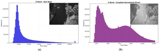
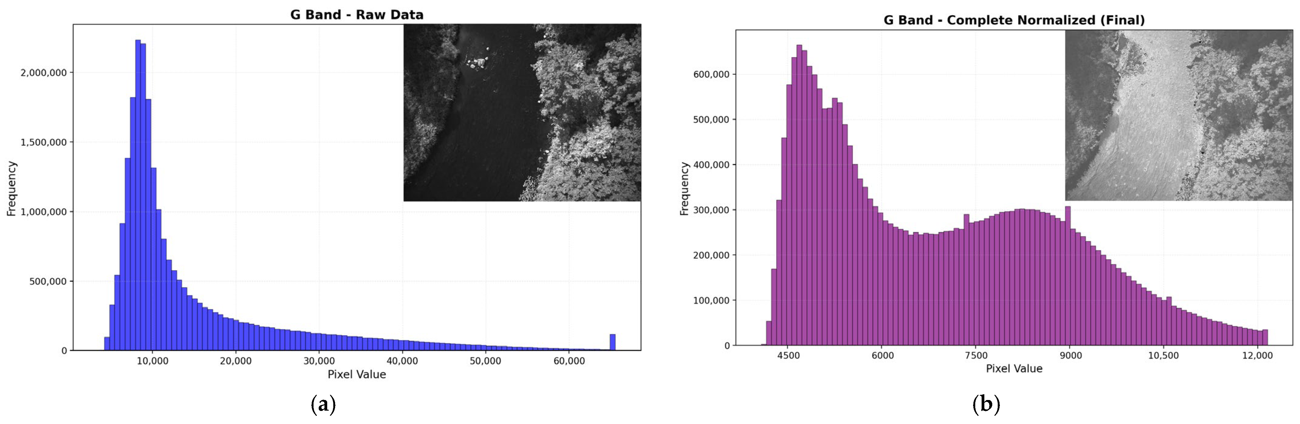
Segmentation masks were used to isolate river regions in multispectral imagery. Each multispectral image was partitioned into two components: one containing only valid river water pixels, and another containing all remaining pixels. Rather than discarding these non-water pixels, an analysis was performed on the valid river water pixels reflectance range. This range was then used as a reference for normalization. The riverbank and outlier pixels were then linearly rescaled so that their values fell within the same interval as the water pixels, ensuring that no non-water region dominated the overall intensity distribution, as seen in Figure 3.

Figure 3. Visual representations of before (a) and after (b) normalization, as well as the pixel value histograms for those representations. After performing image normalization, the pixel value distribution lies within a smaller interval (b) than the raw image (a).

To ensure consistent behavior across the entire dataset, a global reflectance threshold was first computed using only river water pixels extracted from all images. This threshold was determined using a percentile-based approach, which allowed us to remove reflection artifacts. This step was critical for reducing the dynamic range imbalance between water and non-water regions while retaining full spatial coverage.

After filtering and normalization, the processed riverbank and outlier pixels were reintegrated with the original, unmodified river water pixels to reconstruct a complete multispectral image. The resulting image preserved the original spectral relationships within the river while compressing the range of surrounding features. This produced a balanced radiometric representation in which river water details were no longer overshadowed by bright banks or reflective surfaces. The final images contained no missing data, which was essential for robust photogrammetric reconstruction. These normalized images were then used directly as input for point-cloud generation via the SfM workflow.

2.3.3. Structure from Motion

The SfM algorithm is a computer vision technique used to reconstruct a three-dimensional (3D) scene from a set of overlapping two-dimensional (2D) images. The process began with detecting distinctive features and matching them across different images. Accurate correspondences allowed the algorithm to estimate the relative positions and orientations of the cameras, which could be used to triangulate 3D coordinates of the matched points. A global optimization step was then applied, which yielded an optimized set of camera poses and a sparse point cloud, after which a dense reconstruction of the final point cloud began. In this stage, a depth map was computed for every input image using the optimized camera geometry and the sparse point cloud. These depth maps were subsequently fused into a single dense point cloud, which served as the final output of the SfM algorithm. The entire SfM-based 3D point reconstruction process can be summarized mathematically by Equation (5):

$$\lambda X_{3D}=K\left[R\right|t]X_{2D}$$

(5)

Here, $\lambda$ is a scaling factor, K is a camera-intrinsic matrix containing focal lengths and principal points, t is the translation vector (camera position coordinate in real world), and R is the rotation matrix.

For point cloud generation, OpenDroneMap software (version 3.6.0) was used, which was obtained from its official GitHub repository [31] and executed via Docker (version 28.4.0). This software was employed to produce both orthophotos and point clouds from the augmented multispectral images. The processing was performed using ultra-quality feature extraction and point-cloud settings, high-resolution orthophoto and DEM generation at 1 cm resolution, and iterative DEM gap filling. This ensured consistent reconstruction results.

2.3.4. Resulting Data Calibration Using GCPs

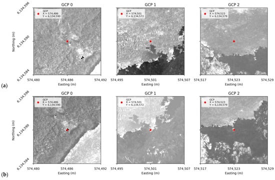
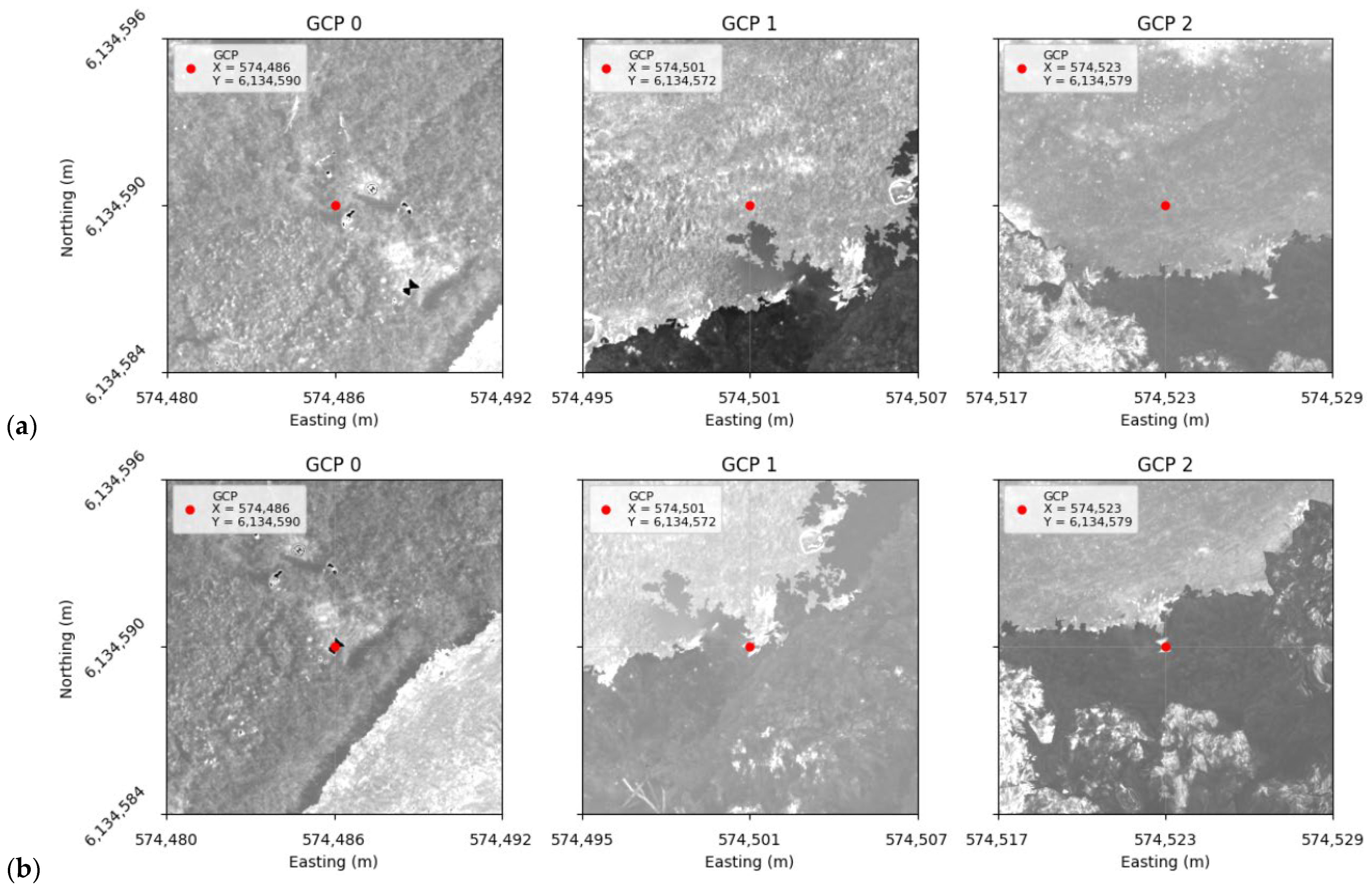
The resulting SfM products were not geographically accurate when referencing them with the known GCPs. This can be seen in Figure 4a. To address this issue, a global affine transformation was applied to the SfM outputs, as can be seen in Equation (6). First, the visual locations of the GCPs were manually identified in the SfM products and associated with their corresponding real-world coordinates. Subsequently, a least-squares formulation was used to estimate the transformation parameters that optimally aligned the visually identified GCPs with their actual GCP coordinates.

$$\begin{array}{cccccc}{x}_1& y_1& 1& 0& 0& 0\\ 0& 0& 0& x_1& y_1& 1\\ ⋮& ⋮& ⋮& ⋮& ⋮& ⋮\\ ⋮& ⋮& ⋮& ⋮& ⋮& ⋮\\ x_n& x_n& 1& 0& 0& 0\\ 0& 0& 0& x_n& y_n& 1\end{array}\times \begin{array}{c}a\\ b\\ \begin{array}{c}c\\ d\\ \begin{array}{c}e\\ f\end{array}\end{array}\end{array}=\begin{array}{c}{x}_1\prime \\ y_1\prime \\ \begin{array}{c}⋮\\ ⋮\\ \begin{array}{c}{x}_n\prime \\ y_n\prime \end{array}\end{array}\end{array}$$

(6)

Figure 4. Factual GCP comparison before (a) and after (b) performing affine transformation on an orthophoto. Red points represent the recorded coordinates for a GCP, while the highly contrasting hourglass shape shows where the point is seen.

Here, $x_n$ and $y_n$ are the visual coordinates for GCP $n$, and $x_n\prime$ and $y_n\prime$ are the factual GCP coordinates. And $a,b,c,d,e,$ and $f$ are the parameters needed to shift a point in the SfM outputs toward correct geographic locations, as can be seen in Equation (7):

$$\begin{array}{c}{x}^{\prime }=a\times x+b\times y+c\\ y^{\prime }=d\times x+e\times y+f\end{array}$$

(7)

The global affine transformation ensured that every visual GCP representation on both orthophotos and point clouds was as close to the true recorded coordinates as possible, while still maintaining coherence between points. The results of this transformation can be seen in Figure 4b.

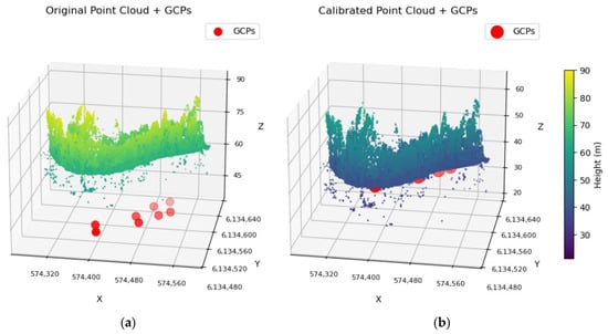
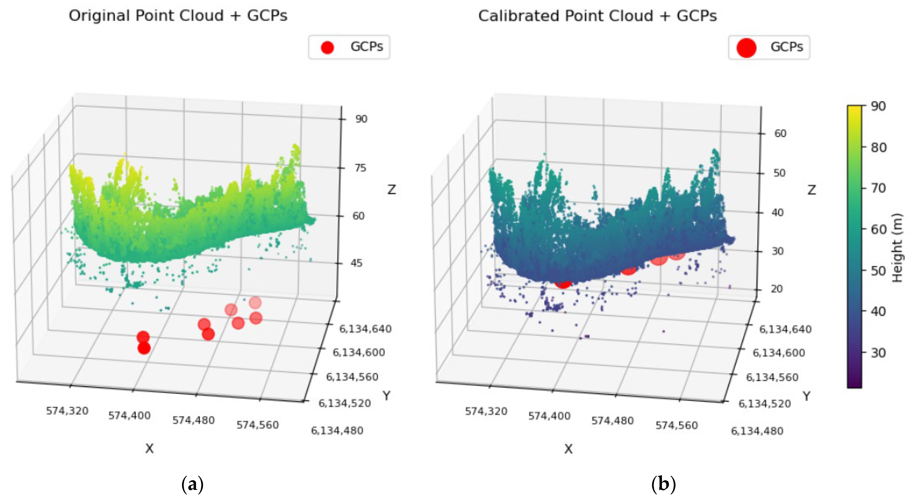
The factual GCP coordinates can be seen directly over the visual GCPs, which indicates that the affine transformation was successful. The same parameters were then also used to shift the SfM-constructed point cloud and the metadata showing how the products of SfM were constructed. After this, the height coordinate for every point in the point cloud was also calibrated, as can be seen in Figure 5.

Figure 5. Point cloud height comparison to GCP height visualization before (a) and after (b).

To correct the point cloud heights, a modified Shepard’s inverse distance weighting (IDW) interpolation, where GCPs were used as a reference, was performed. For each GCP, residuals between the observed point cloud elevations and the known GCP heights were calculated. After this, the Modified Shepard method was used to predict a height correction (delta) at every point, where each neighboring GCP contributed according to a distance-based weight with a specified power parameter and maximum radius. Exact matches were directly assigned to the GCP residual, while points with no neighbors within the radius were assigned to the nearest neighbor delta. Finally, the predicted corrections were applied to the original elevations to generate the calibrated point cloud.

2.4. Depth Estimation

The depth estimation methods explored in this study could be split into two different categories based on the SfM output used by the method. First, physics-based water depth estimation algorithms were applied to preprocessed multispectral orthographic images. Due to their simplicity and ties to the laws of physics, the baseline implementations included classic methods proposed by Lyzenga and Stumpf. Their primary limitation was that both methods required ground-truth data for river depth estimation; therefore other more robust methods were explored in further sections, such as the standard CNN network, which used the same orthographic views and allowed us to set another baseline to evaluate AI-based methods. Furthermore, an adaptive CNN-Stumpf method was implemented, which used a CNN to estimate regression coefficient values, allowing us to apply Stumpf algorithm inferences without actual depth points.

The second part of the study consists of an exploration of geometry-based approaches, such as estimating depth from calibrated point clouds resulting from the SfM algorithm and regression coefficient values, allowing us to apply Stumpf algorithm inferences without actual depth points. Finally, a sequence-based method, which used recurrent neural networks on sequences of images, was proposed and compared to the previously mentioned algorithms. This method utilized the image mapping information that was generated in the 3D reconstruction stages of the SfM algorithm to map pixels from separate images to the same geographic location, which in turn generated the sequence of images needed for this method.

2.4.1. SfM-Based Depth Estimation

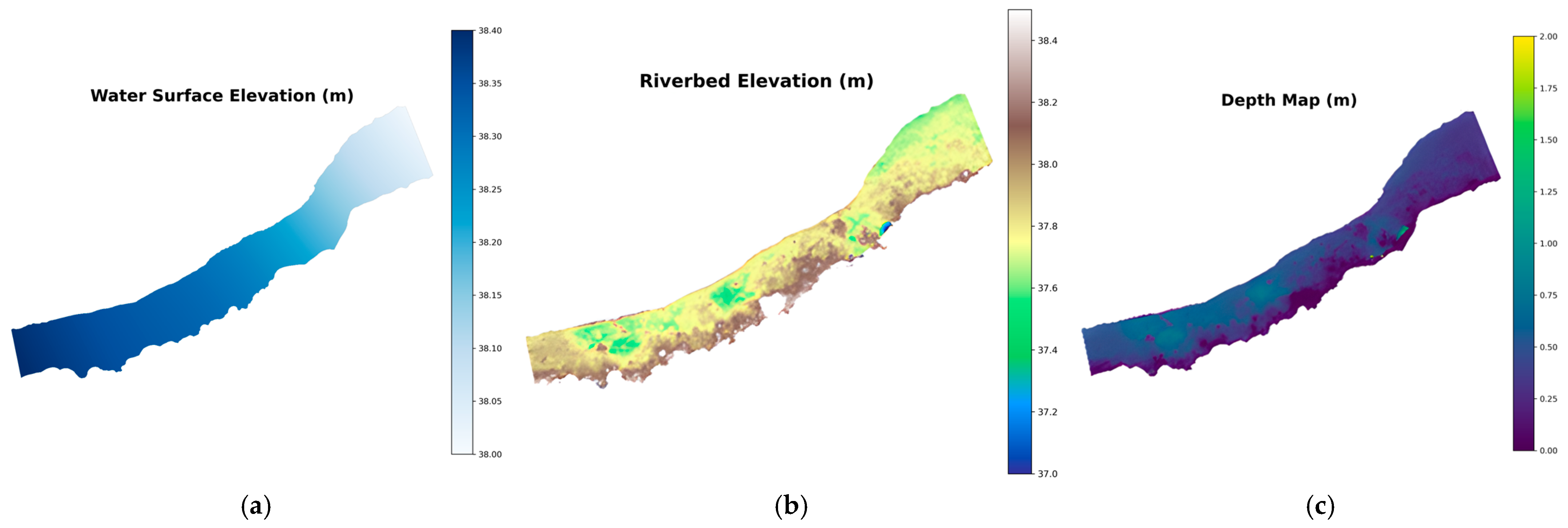
After performing the IDW interpolation to remove the nonlinear distortion along the Z axis, an intermediate depth map was generated directly from the corrected riverbed point cloud. From the corrected point cloud, height information was extracted for each point to generate a DEM, as seen in Figure 6b. This resulted in a digital 2D representation of the riverbed geometry. This representation was then subtracted from the factual water surface height, as seen in Figure 6a, to obtain a heatmap representing the river depths for the entire riverbed, as seen in Figure 6c.

Figure 6. Water surface elevation (a), riverbed elevation (b), and depth map generated from the previous two components (c).

Previous work in water depth estimation using the SfM have found that the calculated depths are usually lower than actual depths due to light refraction when light passes through the water surface [9,18]. This causes the riverbed to appear visually higher in images; therefore, after passing through the SfM, the reconstructed riverbed is also higher than it should be. This is usually solved by multiplying the calculated depth by the light refractive index, which is n = 1.34 between air and clear water.

2.4.2. Lyzenga

The method developed by Lyzenga is one of the most commonly used algorithms for satellite-derived bathymetry. The author proposes that reflectance values captured by sensors vary log-linearly with water depth, as grounded in the Beer–Lambert law [15]. The single-band linear relationship model is described in Equation (8):

$$Z=h_0+h_1\ln \left(R_j-R_{wj}\right)$$

(8)

where Z is the estimated water depth using spectral band j; h₀ and h₁ are the regression intercept and slope values, respectively; R_j is the reflectance value of spectral band j; and R_wj is the reflectance value of optically deep water.

Since the study field is oriented in shallow rivers, optically deep-water values were not present in the data. To be able to implement proposed method, an approach proposed by Flener was adopted, in which optically deep-water reflectance values were not taken into the calculation, enabling the model to be applied in shallow water sources [32].

In practice, light reflectance values are also impacted by other environmental factors, such as water turbidity, sun glare, or atmospheric scattering. To reduce the impact of such conditions, Lyzenga extended the original research by proposing a multiband regression model that integrates information from multiple spectral channels with the goal of minimizing the noise caused by environmental factors [16]. This proposal is described in Equation (9):

$$Z={\beta }_0+\sum _{j = 1}^N{\beta }_j\ln \left(R_j\right)$$

(9)

where Z is the estimated water depth, β₀ is the regression intercept, β_j is the regression coefficient derived from the equation (n), and R_j is the reflectance value of spectral band j. This multiple spectral band combination improves model performance by minimizing the error caused by environment variability.

2.4.3. Stumpf

Another physics-based approach used in this study was proposed by Stumpf, which linearizes the relationship between log-transformed reflectance ratio values and water bottom depth. The calculation for estimated depth using Stumpf’s algorithm is described in Equation (10):

$$Z=m_1· {\displaystyle \frac{\ln \left(R\left({\lambda }_i\right)\right)}{\ln \left(R\left({\lambda }_j\right)\right)}}-m_0$$

(10)

where Z is the estimated water depth, m₁ and m₀ are the regression coefficients, and both R(λ_i) and R(λ_j) are the reflectance values of different spectral bands, ideally with different light reflectance attenuation characteristics. This ratio-based approach was developed to reduce the sensitivity to differences in illumination and river bottom type variability.

The main limitation of the previously mentioned algorithms was their dependence on ground-truth measurements at every location that was being analyzed. Therefore, two unique methods were tested to circumvent these limitations—global calibration Stumpf (GC-Stumpf) and an adaptive CNN-Stumpf blend.

During global calibration, a set of points from multiple rivers was selected with the hope that the coefficients extracted from them would be enough to generalize the model for multiple rivers. Of course, to ensure that the model managed to generalize unseen data, one river was left out of the fitting set and instead was only used for validation.

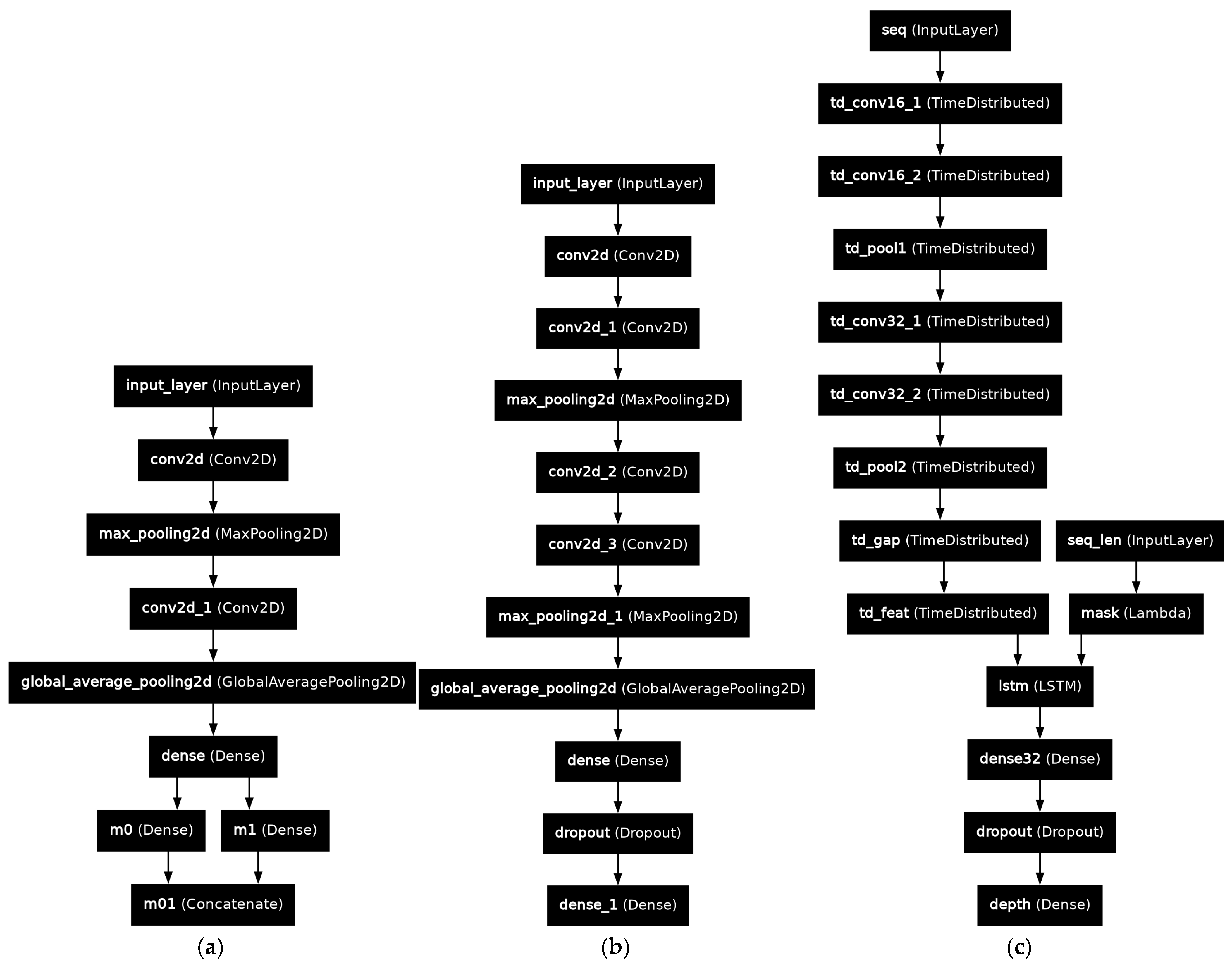
The adaptive CNN-Stumpf model works differently—it does not fit a single set of coefficients. Instead, it uses a convolutional neural network and N × N input images to infer the most suitable set of m0 and m1 values for the given location, as seen in Figure A1a.

2.4.4. CNN-Based Depth Estimation

For the CNN-based depth estimation approach, geographically calibrated orthophotos were used as inputs. For each training and validation sample, a specific ground coordinate in map space was picked, and N × N patches centered around this point were extracted for each available band—green, red, red edge, and NIR. Three additional channels from RGB orthophotos were also included, bringing the final input tensor to N × N × 7. Here, N is any positive integer, with higher values resulting in diminishing returns for accuracy but also increasing computational costs. The generated tensor was then passed to a lightweight convolutional neural network composed of two convolutional blocks, each containing two convolutional layers with ReLU activation functions and a max-pooling layer, followed by a head block with two fully connected layers that estimated the river depth at the center of the patch. The architecture of this model can be seen in Figure A1b.

The model was trained using the Adam optimizer, with a learning rate of 10⁻⁴, mean squared error (MSE) as the loss function, and mean absolute error (MAE) as an additional evaluation metric. Additionally, learning rate reduction on plateau and early stopping were implemented to ensure stable learning, and a checkpoint system was used to save only those weights that provided the lowest validation loss.

The training data were grouped by river, regardless of the date the images of the river were taken. For each river group, a unique model was trained, and the results can be seen in the results analysis. The model did not have access to that river in its training data, only in its validation set—this allowed us to test how well the models’ generalized to unseen rivers.

2.4.5. Sequence-Based Model

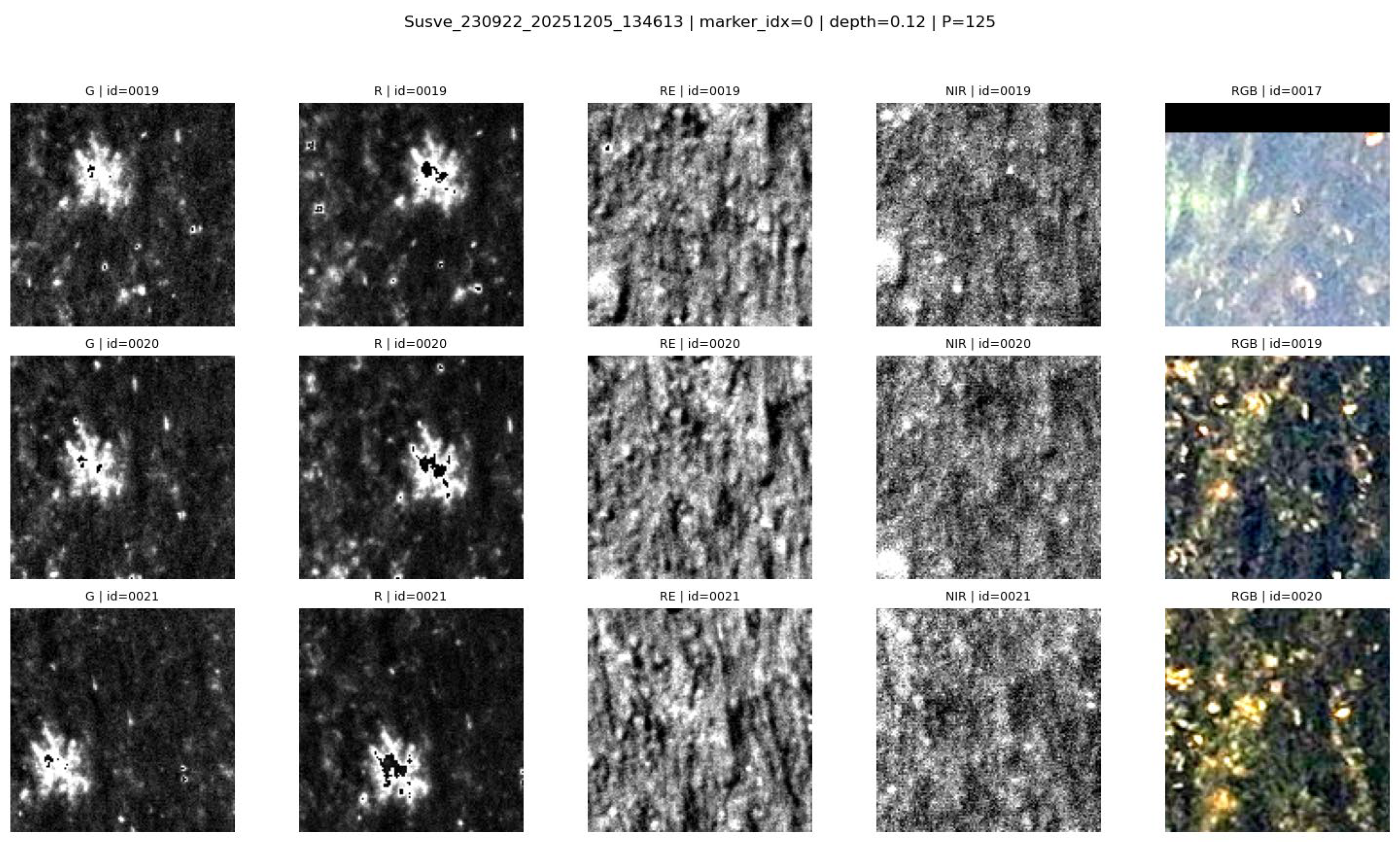
During SfM reconstruction, each 3D point was associated with the corresponding source images and their estimated camera orientation and focal parameters, which were used during point cloud and orthophoto generation. In addition, the resulting DEM could be used to retrieve the approximate height of a specific coordinate. Using this information, the exact pixel locations corresponding to any geographic point could be computed for every image. This procedure is represented by Algorithm 1.

Algorithm 1. World coordinate pixel location extraction from an image

Input: World point coordinate: P_w (X, Y, Z), Camera parameters: Rotation vector r, Translation vector C, Focal rato f, Image width W, Image height H Output: Pixel coordinates in image (u, v) or NULL if point is behind camera 1: Compute focal lengths:   f_x = f * W   f_y = f_x 2. Set central point:   C_x = W/2   C_y = H/2 3. Convert rotation vector r to rotation matrix R_cam->world 4. Compute inverse rotation matrix:   R_world->cam <- transpose(R_cam->world) 5. Transform world point to camera coordinates:   P_c <- R_world->cam * (P_w - C)   (x_c, y_c, z_c) <- P_c 6. If z_c <= 0 then   Return NULL 7: Perform perspective projection   x_n <- x_c/z_c   y_n <- y_c/z_c 8: Convert to pixel coordinates:   u <- f_x * x_n + c_x   v <- f_y * y_n + c_y 9: Return (u, v)

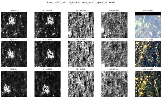
If the resulting pixel location lay within the image boundaries, the image was considered to contain the point; otherwise, it was discarded. This procedure was then performed for every separate image of the river. For every image in which the point was found, a square patch of a specified radius centered on the pixel was extracted, which ultimately was used to visualize the same physical location from multiple angles, as seen in Figure 7.

Figure 7. 125 × 125 frames of the same location.

The extracted patches were then used to create an input tensor of N × N × 7 × M, where N is the patch size and M is the number of patches featuring the point. M patches were ordered chronologically—photos taken earlier were used first. This tensor was passed through an LSTM model, defined in Figure A1c, where a depth value for the center point was returned.

The LSTM mechanism could be replaced by newer algorithms that can process varied sized tensors, such as transformers. However, due to the limited size of the dataset used, a conscious decision was made to use a simpler method that would require less data to train and the results of which would be easier to interpret.

2.5. Results Analysis

For assessing the correctness of the depth estimation method, estimated depths were compared to exact known depths. To evaluate the performance of implemented models, it was decided to calculate the MAE, MSE, and mean absolute percentage error (MAPE) between the calculated depth and factual depth.

$$MAE = {\displaystyle \frac{1}{n}}\sum _{i=1}^n|y_i-\widehat{y}|$$

(11)

$$MSE={\displaystyle \frac{1}{n}}\sum _{i=1}^n{(y_i-{\widehat{y}}_i)}^2$$

(12)

$$MAPE=100{\displaystyle \frac{1}{n}}\sum _{i=1}^n\left|{\displaystyle \frac{y_i-{\widehat{y}}_i}{y_i}}\right|$$

(13)

Here, n is the number of samples, y_i is the ground-truth value, and $\widehat{y_i}$ is the predicted value. Since methods implemented in this study heavily relied on training and fitting processes, a variant of the K-fold cross-validation technique, where each fold was a specific river with all of its occurrences in the training set, was also used. By leaving one river out, the models’ ability to generalize to unseen data became more apparent. This is highly important in all machine learning tasks, but especially in bathymetry, where including a high number of different rivers is infeasible.

Finally, the river images had certain areas that had vegetation or other objects sticking out of the water; therefore, height calculation around these areas tended to be skewed toward the height of those objects. This could cause our chosen mean error values to be increased due to the presence of singular data points that had significantly higher error values compared to all other data points for a river. To account for this issue, it was decided to track the percentage of how many depths point errors lay within certain absolute error ranges. Specifically, thresholds of 10, 20, and 50 cm were chosen. This allowed us to see how accurately a specific depth estimation method performed across all data points in a single river.

3. Results

This section presents an evaluation of the depth estimation approaches introduced in the methodology. All methods were evaluated using the same validation metrics and patch sizes, enabling a fair comparison across different rivers and conditions.

3.1. SfM-Based Depth Estimation Results

This section presents the results of the SfM-based depth estimation approach. For every river, every spectral band present in our dataset was evaluated. The combined results for this method can be seen in Table 2.

Table 2. SfM depth estimation results.

	Band	Light Refraction	MAE (m)	MSE, m2	MAPE, %	<10 cm Error, %	<20 cm Error, %	<50 cm Error, %
Jūra 230713	RGB	1	0.222	0.203	65.165	9.180	79.344	98.361
	RGB	1.34	0.171	0.302	53.611	47.869	91.475	98.361
	RE	1	0.260	0.440	77.922	33.77	72.459	93.77
	R	1	0.615	1.097	285.184	11.803	34.754	59.344
	NIR	1.34	0.652	2.879	160.956	35.410	64.918	80.328
	G	1.34	0.283	0.666	87.563	41.967	73.770	90.492
Jūra 230914	RGB	1	1.614	9.267	305.067	27.053	53.623	60.870
	RE	1	0.873	2.184	190.024	22.705	52.174	61.836
	R	1	0.663	2.492	146.779	28.502	62.802	76.812
	R	1.34	0.924	4.707	200.043	27.053	56.522	67.150
	NIR	1	1.541	7.472	321.965	14.010	38.647	50.242
	G	1	2.278	16.486	455.084	10.628	34.300	46.377
Mūša 240923	RGB	1.34	0.262	0.092	80.410	9.206	54.921	93.016
	RE	1	0.212	0.067	62.681	30.476	57.143	98.095
	R	1	0.233	0.075	74.191	57.563	99.580	100.000
	NIR	1.34	0.316	0.230	79.022	23.810	51.746	85.714
	G	1	0.213	0.065	65.994	27.302	60.635	97.778
Šušvė 230922	RGB	1.34	0.135	0.030	61.675	46.639	88.655	97.479
	RE	1.34	0.067	0.007	31.869	82.773	98.739	100.000
	R	1.34	0.049	0.004	22.934	92.017	99.580	100.000
	NIR	1.34	0.066	0.007	30.180	85.714	98.739	99.580
	G	1	0.085	0.009	37.427	71.429	99.580	100.000
	G	1.34	0.040	0.003	20.061	95.378	99.160	100.000
Šušvė 240626	RGB	1.34	0.145	0.029	62.883	29.670	86.813	98.901
	RE	1.34	0.155	0.075	68.674	63.736	83.516	92.308
	R	1.34	0.059	0.094	27.418	81.319	96.703	100.000
	NIR	1.34	0.212	0.123	93.209	40.659	80.220	89.011
	G	1.34	0.071	0.026	34.693	81.319	96.703	98.901

Applying the light refraction index of n = 1.34 generally improves the depth estimation results. This can especially be seen in both stretches of the Šušvė river, where applying this index on the depths estimated from the Šušvė 230922 G band causes the MAE to be cut in half. In addition, the number of points that have error values below 10 cm increases from 71.429% to 95.378%.

To better understand these results, specific SfM reconstruction cases were further examined through representative case studies. The following subsections provide a more detailed examination of the conditions under which SfM reconstructions perform poorly, as well as where this method demonstrates improved accuracy.

3.1.1. Worst Reconstruction Cases

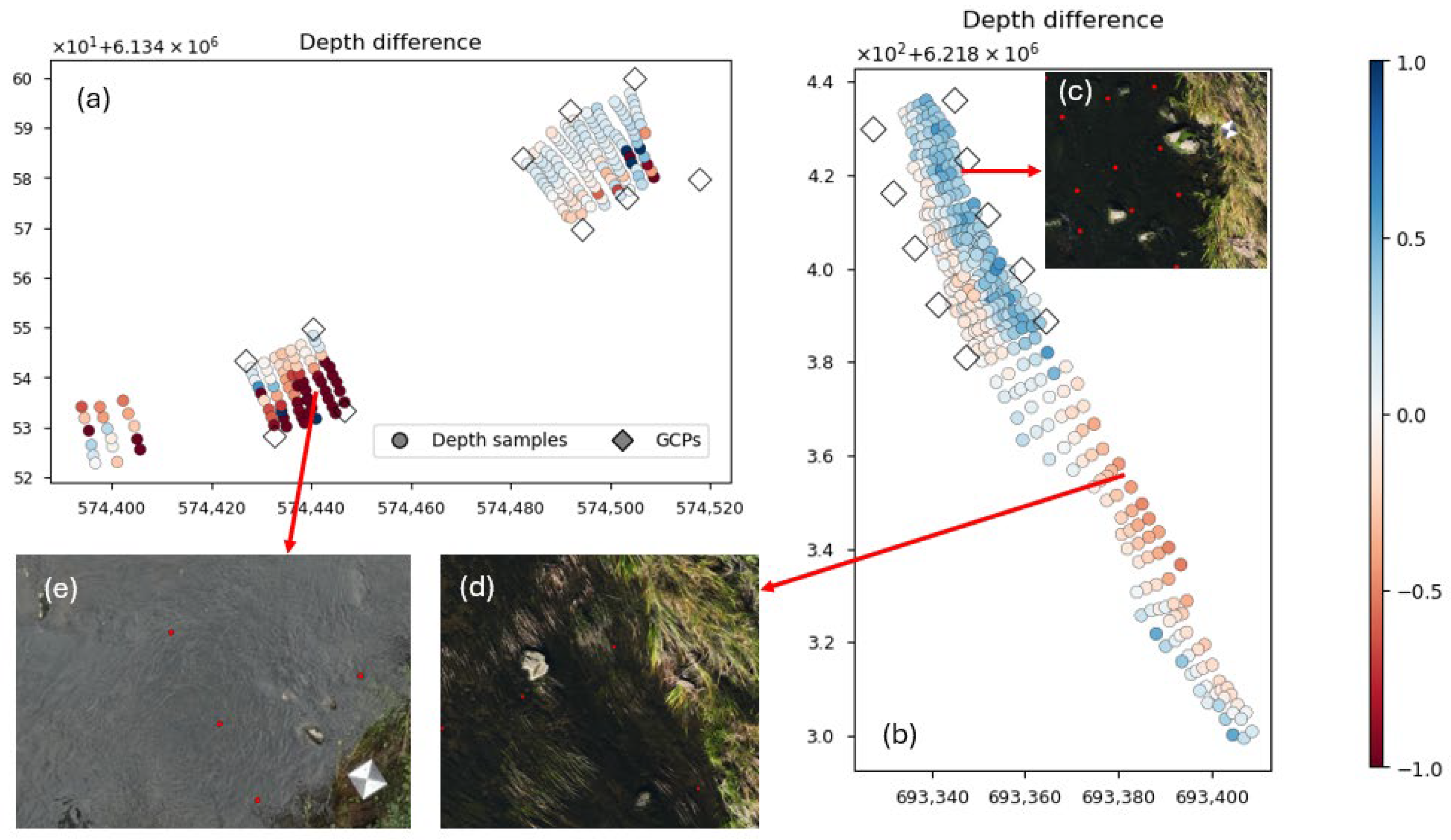
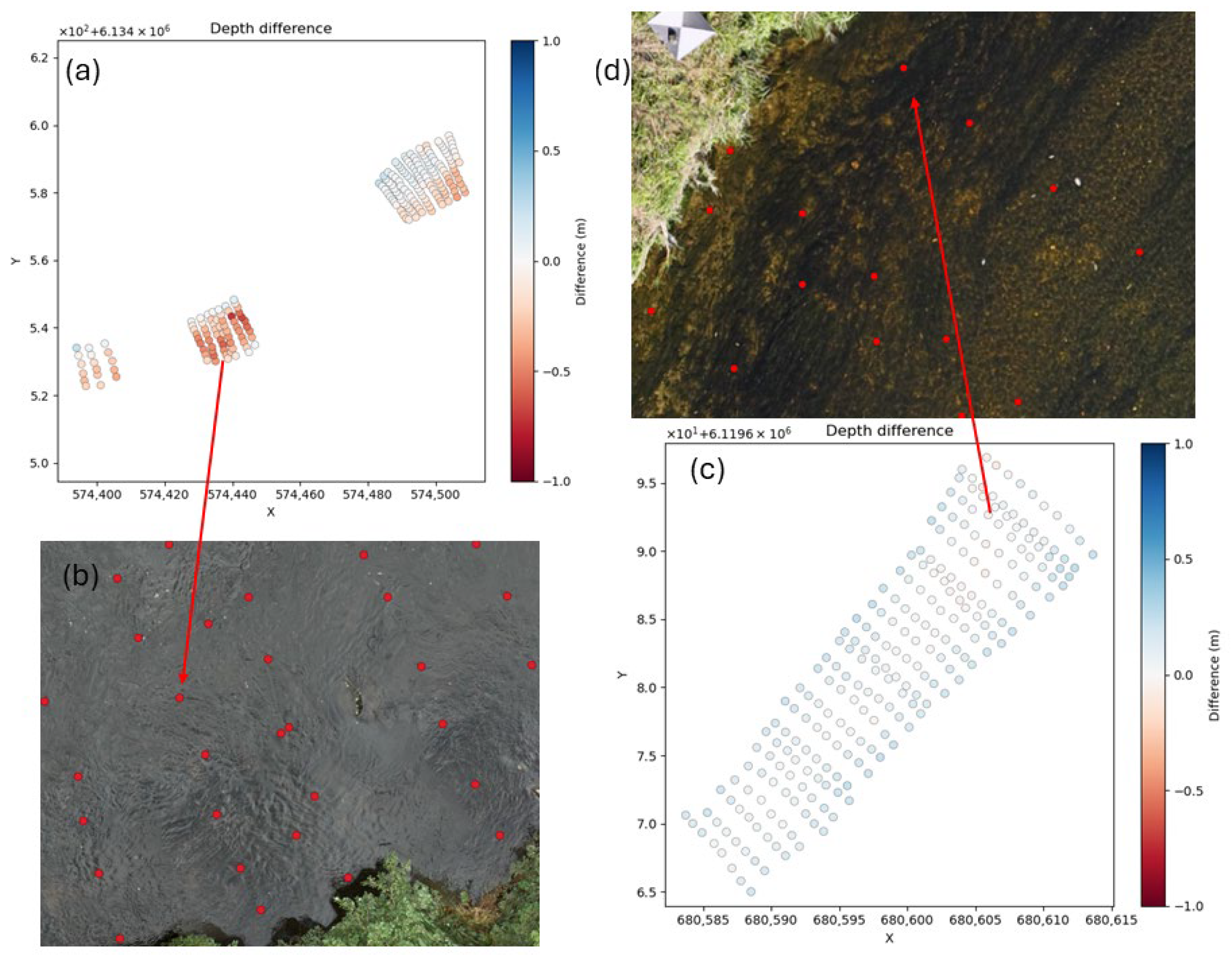
The two worst SfM reconstructions are for the Mūša 240923 and Jūra 230914 rivers. The result visualizations for both rivers can be seen in Figure 8.

Figure 8. SfM depth estimation results for Jūra 230914 (a) and Mūša 240923 (b). A darker blue color shows that the predicted depth is less than the factual depth. A darker red color shows that the predicted depth is greater than the factual depth. Figure (c) shows boulders protruding from the river, which cause the SfM algorithm to incorrectly reconstruct the surrounding area. Figure (d) shows vegetation growing out of the river, which causes the SfM algorithm to incorrectly reconstruct the surrounding area. Figure (e) shows the water clarity of the water, where large errors are made when trying to calculate the depth from the reconstructed point cloud. Red dots in Figure (c–e) show locations of known depth point locations.

Both rivers have large error values in various portions of their respective rivers, as can be seen in Figure 8a,b. The errors for the Mūša river are mainly caused by vegetation and various objects like boulders protruding from the river, as can be seen in Figure 8c,d. These obstacles cause the SfM to reconstruct the surrounding river areas at their height, which usually means that the reconstructed riverbed is above the water surface, causing the estimated depth of those areas to be negative. The complete opposite issue can be seen in the Jura 230914 river, where due to the clarity of the river, the SfM algorithm cannot see the riverbed, which causes the algorithm to reconstruct this area as much deeper than it should be. Since in both scenarios the depths of large areas of the river are either negative or significantly greater than the actual depth, applying the light refraction index further increases the error of these rivers.

3.1.2. Mixed Reconstruction Case

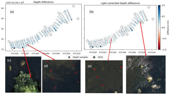
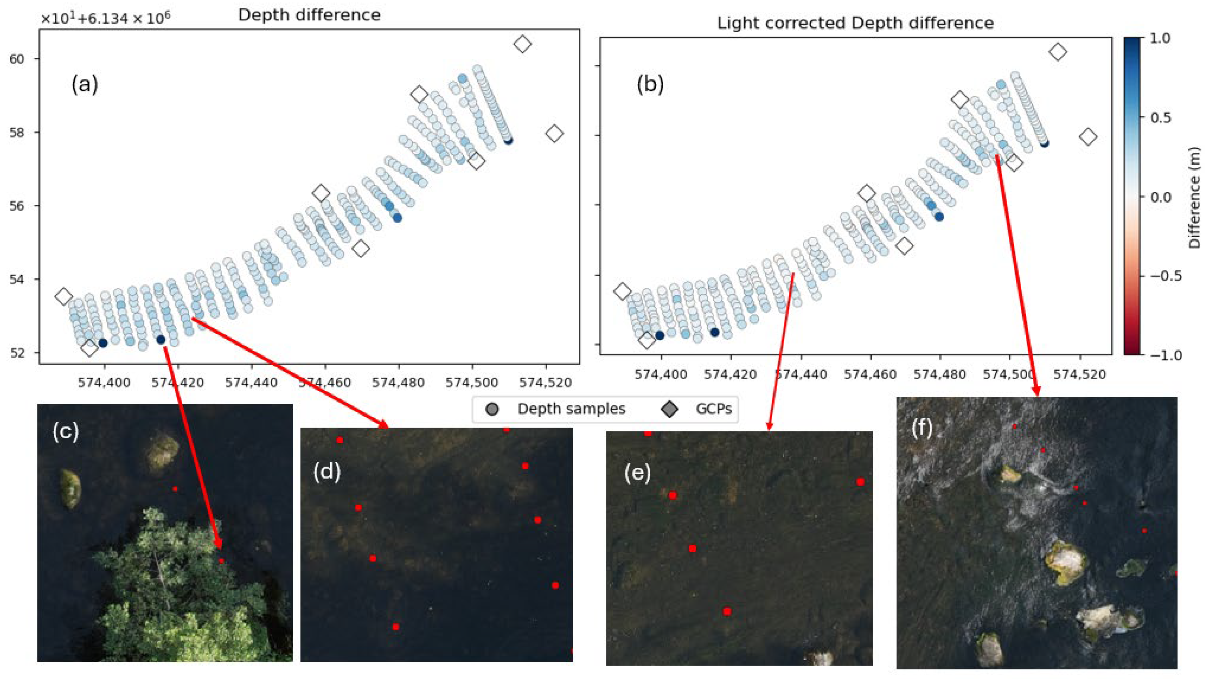
If the SfM reconstruction of a riverbed is correct, the estimated depth should be positive and slightly lower than the factual depth. After applying the light refraction index, the estimated depth should fall closer to the factual depths. This can be seen in the reconstruction of Jūra 230713 in Figure 9. This can also be seen in Table 2, where this river initially has 9.180% of its reconstructed points fall below 10 cm error, but after applying the light refractive index, this percentage increases to 47.869%.

Figure 9. SfM depth estimation results for Jūra 230713. Figure (a) shows the results for the uncorrected point cloud. Figure (b) shows the light refraction-corrected results. Figure (c) shows an overhanging tree blocking a delph point. Figures (d,e) show the comparison of depth errors in shaded and brightly lit areas. Figure (f) shows boulders protruding from the river surface alongside water ripples, which causes the surrounding area to have larger error values.

The Jūra 230713 river also has many of the problems seen in the Mūša river and the other Jūra river. Figure 9f shows boulders protruding from the water surface, as well as water ripples, which likely cause the reconstructed riverbed in that area to be above the water surface. Additionally, the bottom shore of this river has trees covering some of the depth points, which caused some of those depth points to have the height of those trees. Finally, due to those trees, portions of the river are shaded, as seen in Figure 9d. These shaded areas also tend to have higher error values compared to brightly lit areas, as can be seen in Figure 9e.

3.1.3. Best Reconstruction Case

Point clouds that use multispectral bands for 3D reconstruction generally achieve significantly higher accuracy. This can specifically be seen in both stretches of the Šūšvė river, where even the worst performing multispectral bands have about double the number of points that fall within an error range below 10 cm compared to that of a point cloud reconstructed using RGB images. Out of all the used bands, the green and red bands generally perform the best. This is the expected result, since those two bands have the highest water penetration out of the used bands. Under ideal conditions, the SfM algorithm reconstructs a riverbed with minimal errors, as can be seen in Figure 10.

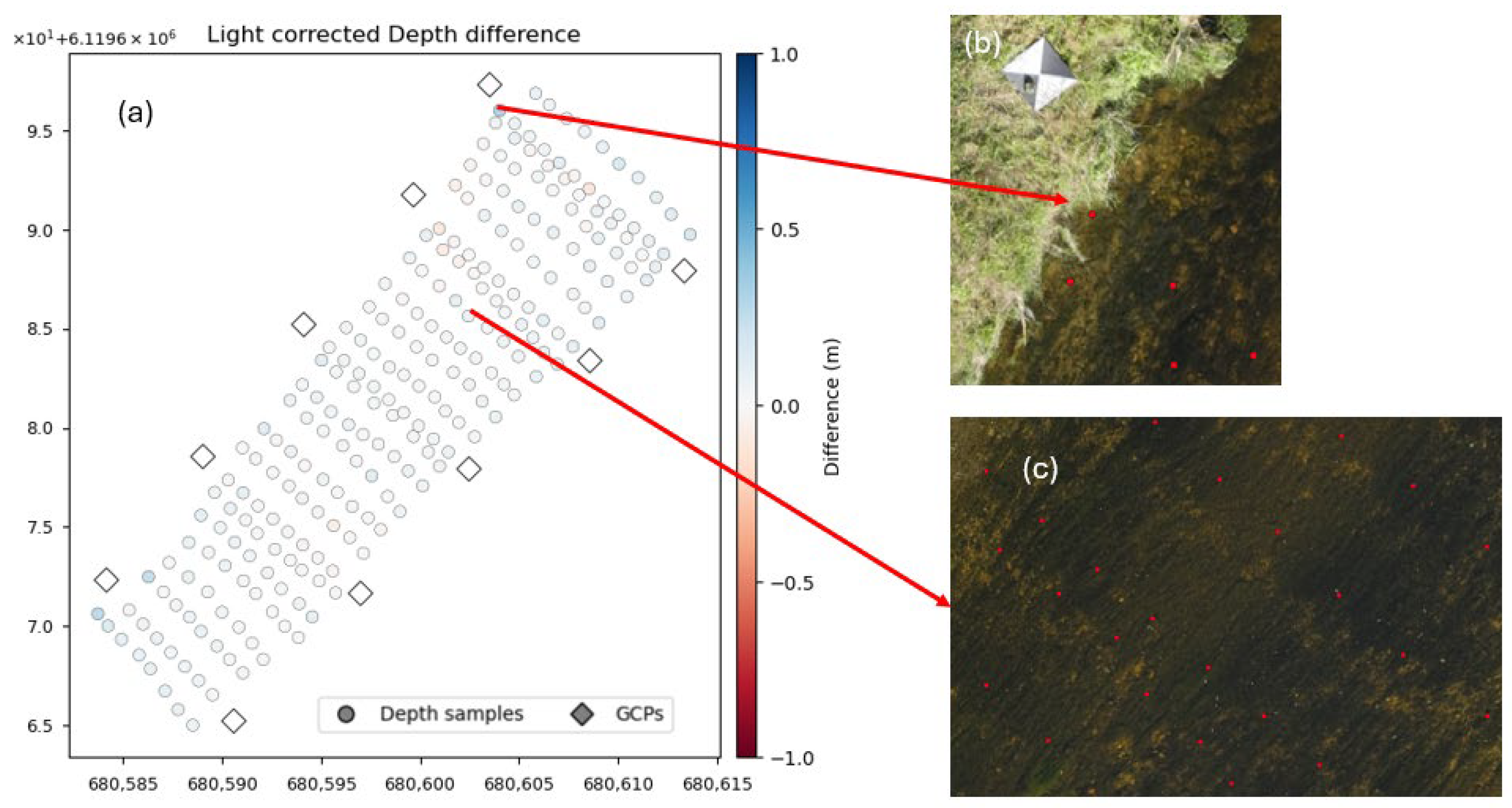
Figure 10. SfM depth estimation results for Šušvė 230922 (a). Figure (b) shows a point close to the shore of the river, which has the largest error value out of all the depth points. Figure (c) shows the water clarity, which has error values close to zero.

The Šušvė river does not have any of the problems present in the other rivers. There are not any boulders or other objects protruding from the river, which could cause the reconstruction to appear above the water surface. In addition, the riverbed is clearly visible, which likely contributes to almost perfect reconstructions of this river. Points that have the highest error values are generally very close to the shore, where the riverbank height, as well as the shifts in x- and y-coordinates during the 3D reconstruction of the entire river, likely cause the height values of these points to be closer to or at ground surface height.

3.2. Image-Based Depth Estimation Results

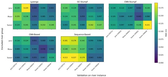
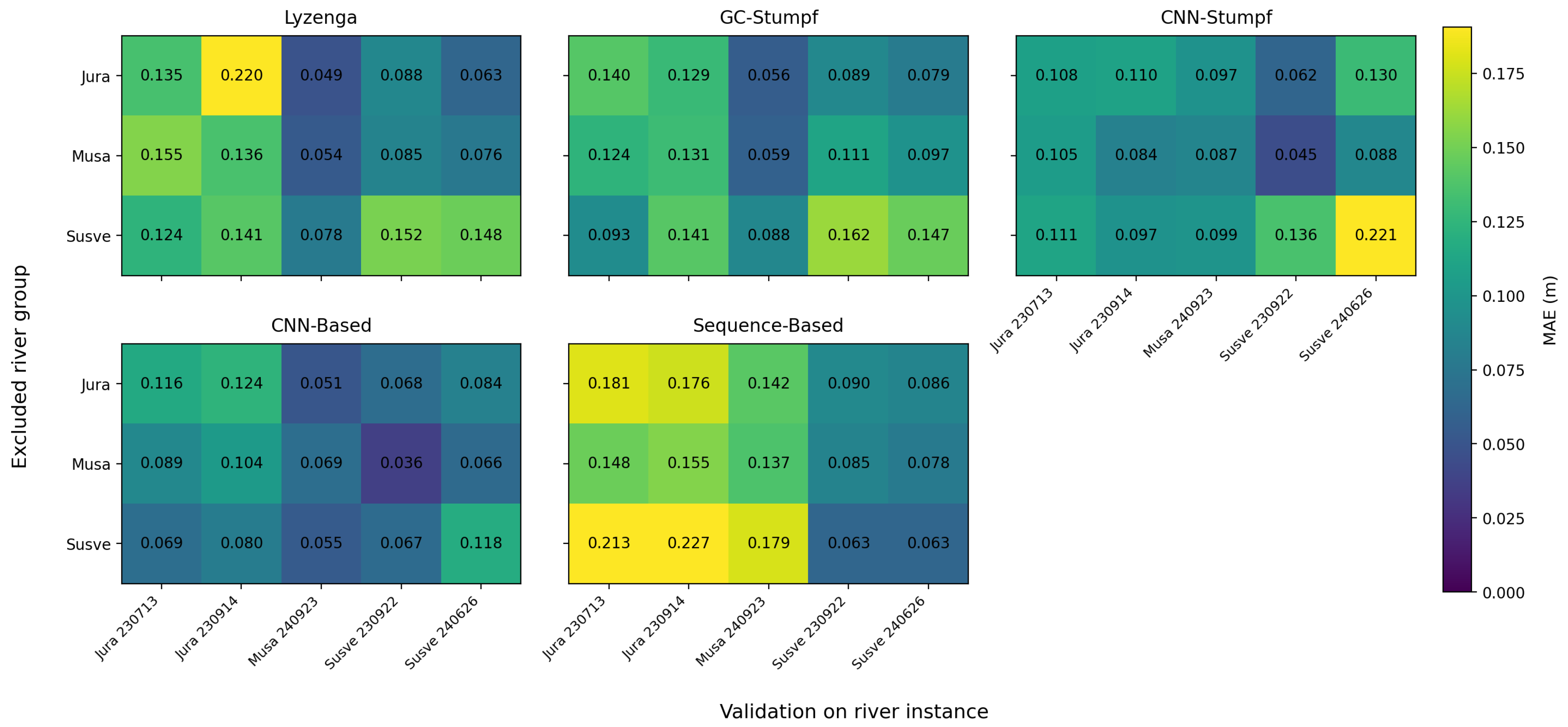
This section presents the results of all five image-based depth estimation methods. As described in the results analysis section, to evaluate the performance of each of these methods, a leave-one-river-out cross-validation strategy was applied to evaluate the performance of each method, the results of which can be seen in Figure 11. In this figure, each row represents a river, which has been excluded from training, while each column indicates the evaluation results for a specific river subset.

Figure 11. MAE matrices for Lyzenga, GC-Stumpf, CNN-Stumpf, CNN, and sequence-based depth estimation methods.

This unified presentation highlights the main cross-river generalization patterns without repeating fold-level descriptions for each method separately.

3.2.1. Physics-Based Depth Estimation Results

Following an initial spectral analysis, the green and red bands were selected for the implementation of the Lyzenga model. As expected, the performance varies between rivers and it is sensitive to changes in the environment, such as water turbidity, illumination, or vegetation coverage. The performance of GC-Stumpf is slightly more consistent across rivers. However, just like Lyzenga, the performance of the model is still highly reliant on environmental conditions. Nevertheless, in addition to Lyzenga, these results establish a physics-based baseline for further evaluation. To address the environmental conditions, an adaptive CNN-Stumpf model was also developed. It estimated the optimal m₀ and m₁ values for any given patch before applying the Stumpf equation. While this model results in overall improved performance, it still struggles to generalize consistently, which is especially noticeable for the Šušvė river. This suggests that the addition of adaptive parameter estimation is not sufficient to fully compensate for environmental variables.

Overall, the physics-based approach shows that the incorporation of physical relationships alone is not enough to ensure consistent results, especially when encountering inconsistent variables in the environment.

3.2.2. CNN-Based Depth Estimation Results

The CNN-based model manages to achieve better results than the previously explored physics-based models, including the inherently similar CNN-Stumpf model, which severely underperforms on the Šušvė river.

The fold-level results also suggest that the contribution of each river to the training set is not uniform. For example, the exclusion of Mūša has the least impact on the results, whereas the exclusion of Jūra or Šušvė has higher impacts on the MAE.

These results indicate that the ability to capture broader spatial context, including vegetation, reflection and local texture cues, is more important for depth estimation than relying on predefined spectral relationships.

3.2.3. Sequence-Based Model Depth Estimation Results

Because sequence-based models can use multiple images of the same physical location, there were high hopes for this model. However, the alignment errors, which vary from photo to photo, introduced while extracting patches mean that an exact representation of the measured point is not possible, in turn making precise estimation infeasible. Nevertheless, the model still manages to train and estimate depth in the area, rather than a precise point. In most cases, with the exception of Šušvė, this sort of estimation is not as efficient as the CNN model, which used a preprocessed orthophoto as the source image.

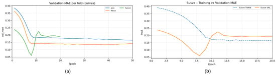
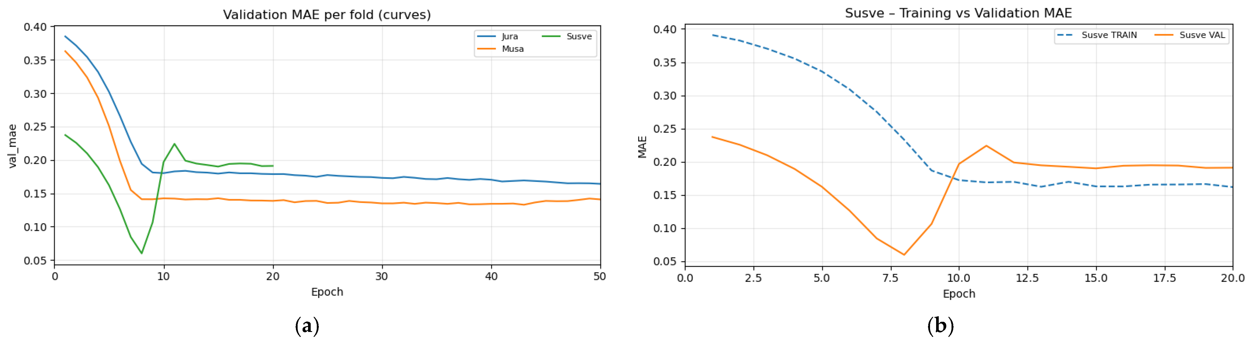
Another issue that is apparent in this model is overfitting—some folds quickly lose the ability to generalize for unseen data. This is illustrated in Figure 12.

Figure 12. Training history MAE. (a) All folds and (b) Šušvė validation and training MAE.

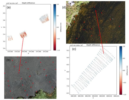
For this reason, all model inference was performed using the weights of the lowest validation MAE. Regardless of these limitations, the sequence-based model manages to outperform the CNN model on the Šušvė river. This is consistent with earlier observations that Šušvė allows for more accurate point cloud generation, which in turn makes coordinate-to-pixel mapping more reliable across multiple images. The opposite is seen with Mūša and Jūra, where this mapping is less accurate. This can be seen in Figure 13.

Figure 13. Sequence-based model depth estimations for Jūra 230914 (a) showcasing unclear riverbed due to turbulent water (b) and depth estimation for Šušvė 230922 (c) showing clearly visible riverbed (d).

The turbulent water in Jūra leads to a worse riverbed reconstruction during previous steps, making the mapping of geographic coordinates and pixel locations less accurate. Whereas in the example of Šušvė, the model manages to achieve higher accuracy since it is easier to reference the same spot consistently. This leads to the conclusion that improving upon the precision of the algorithm used to map coordinates to pixels in separate images would also lead to improved results in a sequence-based model, making the sequence-based model more accurate than the others explored in the paper.

Overall, these findings highly suggest that a sequence-based approach is limited by the precision of the coordinate-to-pixel mapping workflow. Any improvements made upon this algorithm would most likely improve the final quality of the model and allow it to outperform the CNN model in other rivers as well.

3.3. Results Summary

Table 3 summarizes the results that were obtained for each river using each of the tested methods and highlights the best performing ones. For methods that created models to predict water depth from light reflection values at image points, the presented results are for those methods that exclude the selected river depth predictions.

Table 3. Depth estimation method results comparison.

Method	MAE, m	MSE, m2	MAPE, %	<10 cm Error, %	<20 cm Error, %	<50 cm Error, %
Jūra
Lyzenga	0.188	0.057	43.109	32.813	63.672	95.508
GC-Stumpf	0.133	0.031	34.657	47.887	76.995	99.061
CNN-Stumpf	0.127	0.027	35.793	48.828	80.078	99.609
CNN	0.132	0.029	35.048	49.023	78.516	99.219
Sequence	0.179	0.054	41.660	38.281	63.281	96.875
SfM	0.171	0.302	53.611	47.869	91.475	98.361
Mūša
Lyzenga	0.138	0.035	33.875	52.063	75.556	97.778
GC-Stumpf	0.129	0.028	36.408	49.673	80.719	99.673
CNN-Stumpf	0.117	0.026	32.615	59.683	80.000	99.048
CNN	0.113	0.025	27.604	58.095	81.270	99.365
Sequence	0.137	0.034	34.651	50.794	76.825	97.778
SfM	0.212	0.067	62.681	30.476	57.143	98.095
Šušvė
Lyzenga	0.139	0.027	74.994	35.029	78.443	100.000
GC-Stumpf	0.142	0.025	72.057	26.199	80.074	100.000
CNN-Stumpf	0.142	0.030	69.419	39.820	74.551	100.000
CNN	0.083	0.011	37.861	67.665	95.808	100.000
Sequence	0.063	0.006	29.818	79.940	99.401	100.000
SfM	0.040	0.003	20.061	95.378	99.160	100.000

As can be seen from the table above, no single method dominates across all river groups. SfM performs exceptionally well on the Šušvė river since its riverbed is better suited for point cloud reconstruction. This method manages to capture 95% of the river with less than 10 cm error. However, this method does not manage to recreate this success on different rivers, especially Mūša.

The models that best perform on Mūša and Jūra are the CNN and adaptive CNN-Stumpf models. They both perform similarly well on these rivers due to their very similar architecture—the only difference between the two being an explicit link to a physics-based equation in the adaptive CNN-Stumpf model, whereas the CNN model directly estimates depth. The worst performing models turn out to be Lyzenga and GC-Stumpf—they do not generalize well to unseen data due to their reliance on river-specific parameters, such as water quality, illumination, or even vegetation quantity. Finally, the sequence-based model falls right in between the best and worst performing models. Its reliance on point clouds means that it performs very well on Šušvė, outperforming the CNN model, but it struggles to reach higher accuracy where point cloud reconstructions are not as accurate.

4. Discussion

The results of the data normalization demonstrated that balancing multispectral imagery is a critical preprocessing step for reliable river reconstruction. The findings showed that unnormalized multispectral data led to feature dominance by bright riverbank elements and incomplete riverbed reconstruction. By normalizing non-water pixels to the range of river water, while preserving full spatial coverage, the proposed approach enhanced water-related features without suppressing contextual information required for stable matching. This supports the working hypothesis that improving radiometric consistency across the scene directly benefits Structure-from-Motion–based depth estimation in fluvial environments. Future work could explore adaptive or physics-based normalization strategies that account for varying illumination conditions and water turbidity.

Depth estimation based on SfM-derived point clouds performed well under favorable conditions, as demonstrated by the results from the Šušvė river. However, the presence of unfavorable conditions, such as protruding objects and poor riverbed visibility, substantially hindered the accurate reconstruction of riverbed topography, as observed in the results for the Jūra and Mūša rivers. Depth estimates derived from multispectral imagery generally outperformed those obtained from RGB imagery. Applying a light refractive index correction with n = 1.34 to the estimated depths generally reduced depth estimation errors in cases where the riverbed was reconstructed correctly. However, this correction was ineffective when the reconstructed riverbed was reconstructed above the water surface or below the factual riverbed height. Overall, SfM-based depth estimation was most effective for small, clear, and unobstructed river segments. For larger areas, computational costs increased substantially. Moreover, the method performed poorly in rivers with dense vegetation, poor riverbed visibility, or with numerous objects, such as boulders, protruding above the water surface.

Physics-based methods, such as Lyzenga and GC-Stumpf, gave a useful baseline for estimating shallow water depth. Their performance was closely tied to river-specific optical properties, such as water clarity, bottom composition, and illumination conditions. Because of this, they performed well under similar conditions to the ones seen during calibration. However, their reliance on globally fitted parameters limited their ability to generalize to rivers with different environmental characteristics. Evaluations across multiple rivers confirmed that even moderate variations in water quality or surrounding vegetation led to a noticeable degradation in performance, which showed the inherent constraint of purely physics-driven formulations in heterogeneous river environments.

The confirmed advantage of machine learning–based approaches lies in their ability to incorporate local spatial context. The CNN model, which operated on small image patches extracted from geographically aligned orthophotos, consistently achieved lower errors across diverse river conditions compared to physics-based baselines. This suggests the importance of contextual visual cues, such as texture, shading patterns, and local contrast between the riverbed and water surface. These features play a significant role in depth estimation. This improvement was not driven by increased model complexity, but rather by the careful alignment of multispectral inputs, controlled window sizes, and strict validation using leave-one-river-out evaluation. These results support the interpretation that incorporating local visual context is essential for robust depth estimation in real-world river settings where optical conditions vary spatially and temporally.

Sequence-based models aim to improve depth estimation by incorporating multi-view contextual information; however, their performance is primarily constrained by the accuracy of geometric alignment. Because coordinate-to-pixel mapping relies on SfM-derived point clouds, even small spatial errors introduce inconsistencies between image patches representing the same physical location. As a result, additional views do not always improve performance and may instead introduce conflicting information. This explains the strong dependency on river conditions: the model performed well when point cloud reconstruction was accurate (e.g., Šušvė), where this model outperformed the CNN model, but degraded significantly when vegetation, turbidity, or shading reduced reconstruction quality (e.g., Jūra and Mūša). These findings indicate that the current limitation lies not in the sequence-based modeling approach itself but in the reliability of cross-view alignment. Future improvements are therefore most likely to arise from advances in point cloud generation, refinement of SfM calibration procedures, or alternative strategies for establishing cross-view correspondence without relying exclusively on dense geometric reconstruction.

5. Conclusions

This study highlights the importance of data radiometric normalization in enhancing multispectral data for reliable SfM-based river bathymetry reconstruction. Adjusting non-water pixels to the radiometric range of water proved effective in mitigating feature dominance from bright surfaces and improving depth estimation.

Traditional physics-based methods performed well only when applied to familiar conditions, lacking generalizability. Photometry-based depth estimation methods were strongly influenced by environmental conditions. By contrast, machine learning models, particularly convolutional neural networks (CNNs), achieved the most consistent and accurate overall results across diverse river conditions.

While sequence-based models offer theoretical advantages by leveraging multi-angle spatial context, their performance is highly dependent on data quality. They outperformed CNNs only in ideal scenarios (e.g., Šušvė), but generally underperformed in more complex environments (e.g., Jūra) due to image misalignment from low-quality point clouds, likely caused by identified positional inaccuracies in SfM outputs.

Improving point cloud accuracy or developing more reliable pixel-to-coordinate mapping methods is essential for unlocking the full potential of multi-view–based approaches. Enhancements in these areas would increase spatial consistency across views and preserve crucial visual information, ultimately leading to more reliable depth estimation in challenging environments.

References

- Pathan, A.I.; Patel, D.; Samal, D.R.; Prieto, C.; Eslamian, S. River Bathymetry acquisition techniques and its utility for river hydrodynamic modeling. In Handbook of HydroInformatics: Volume III: Water Data Management Best Practices; Elsevier: Amsterdam, The Netherlands, 2023; pp. 339–351. [Google Scholar] [CrossRef] [Scilit]
- Arseni, M.; Voiculescu, M.; Georgescu, L.P.; Iticescu, C.; Rosu, A. Testing Different Interpolation Methods Based on Single Beam Echosounder River Surveying. Case Study: Siret River. ISPRS Int. J. Geo-Inf. 2019, 8, 507. [Google Scholar] [CrossRef] [Scilit]
- Kasvi, E.; Salmela, J.; Lotsari, E.; Kumpula, T.; Lane, S.N. Comparison of remote sensing based approaches for mapping bathymetry of shallow, clear water rivers. Geomorphology 2019, 333, 180–197. [Google Scholar] [CrossRef] [Scilit]
- Jiang, H.; Rutherfurd, I. Potential to use free satellite imagery to retrieve the past bathymetry of large rivers. Remote Sens. Appl. 2024, 33, 101133. [Google Scholar] [CrossRef] [Scilit]
- Maps of Water Depth Derived from Satellite Images of Selected Reaches of the American, Colorado, and Potomac Rivers Acquired in 2020 and 2021 (ver. 2.0, September 2024). Available online: https://www.sciencebase.gov/catalog/item/66c78ca2d34e0338828b41fa (accessed on 23 September 2025).
- Ai, B.; Wen, Z.; Wang, Z.; Wang, R.; Su, D.; Li, C.; Yang, F. Convolutional neural network to retrieve water depth in marine shallow water area from remote sensing images. IEEE J. Sel. Top. Appl. Earth Obs. Remote Sens. 2020, 13, 2888–2898. [Google Scholar] [CrossRef] [Scilit]
- Kutser, T.; Hedley, J.; Giardino, C.; Roelfsema, C.; Brando, V.E. Remote sensing of shallow waters—A 50 year retrospective and future directions. Remote Sens. Environ. 2020, 240, 111619. [Google Scholar] [CrossRef] [Scilit]
- Wang, E.; Li, D.; Wang, Z.; Cao, W.; Zhang, J.; Wang, J.; Zhang, H. Pixel-level bathymetry mapping of optically shallow water areas by combining aerial RGB video and photogrammetry. Geomorphology 2024, 449, 109049. [Google Scholar] [CrossRef] [Scilit]
- Dietrich, J.T. Bathymetric Structure-from-Motion: Extracting shallow stream bathymetry from multi-view stereo photogrammetry. Earth Surf. Process. Landf. 2017, 42, 355–364. [Google Scholar] [CrossRef] [Scilit]
- Szostak, B.; Specht, M.; Burdziakowski, P.; Stateczny, A.; Specht, C.; Lewicka, O. Methodology for performing bathymetric measurements of shallow waterbodies using an UAV, and their processing based on the SVR algorithm. Measurement 2023, 223, 113720. [Google Scholar] [CrossRef] [Scilit]
- Rossi, L.; Mammi, I.; Pelliccia, F. UAV-Derived Multispectral Bathymetry. Remote Sens. 2020, 12, 3897. [Google Scholar] [CrossRef] [Scilit]
- Shen, Q. Estimation of Water Depth from Multispectral Drone Imagery: A Suitability Assessment of CNN Models for Bathymetry Retrieval in Shallow Water Areas. Master’s Thesis, KTH Royal Institute of Technology, Stockholm, Sweden, 2022. [Google Scholar]
- Shen, Q.; Mahima, K.T.Y.; De Zoysa, K.; Mottola, L.; Voigt, T.; Flierl, M. CNN-Based Estimation of Water Depth from Multispectral Drone Imagery for Mosquito Control. In 2023 IEEE International Conference on Image Processing (ICIP); IEEE: Piscataway, NJ, USA, 2023. [Google Scholar] [CrossRef] [Scilit]
- Mandlburger, G.; Kölle, M.; Nübel, H.; Soergel, U. BathyNet: A Deep Neural Network for Water Depth Mapping from Multispectral Aerial Images. PFG J. Photogramm. Remote Sens. Geoinf. Sci. 2021, 89, 71–89. [Google Scholar] [CrossRef] [Scilit]
- Lyzenga, D.R. Remote sensing of bottom reflectance and water attenuation parameters in shallow water using aircraft and landsat data. Int. J. Remote Sens. 1981, 2, 71–82. [Google Scholar] [CrossRef] [Scilit]
- Lyzenga, D.R.; Malinas, N.P.; Tanis, F.J. Multispectral bathymetry using a simple physically based algorithm. IEEE Trans. Geosci. Remote Sens. 2006, 44, 2251–2259. [Google Scholar] [CrossRef] [Scilit]
- Pan, L.; Baráth, D.; Pollefeys, M.; Schönberger, J.L. Global Structure-from-Motion Revisited. Available online: https://github.com/colmap/glomap (accessed on 18 November 2025).
- Witek, M.; Walusiak, G.; Halicki, M.; Remisz, J.; Borowicz, D.; Parzóch, K.; Kasprzak, Ł.; Langhammer, J.; Gallay, M.; Miřijovský, J.; et al. Reconstructing bed topography of a shallow river from close-range aerial imagery: Multi-UAV experimental campaign in the Izera river (SW Poland/N Czechia). Geomorphology 2025, 471, 109544. [Google Scholar] [CrossRef] [Scilit]
- You, H.; Kim, D.; Gwon, Y. Morphological Dune Mapping in Shallow Alluvial Stream Using UAV-Based Hyperspectral Images. KSCE J. Civ. Eng. 2024, 28, 1594–1606. [Google Scholar] [CrossRef] [Scilit]
- Das, S.; Salimi Tari, S. Deep Learning for Efficient Riverine Bathymetry Inversion. In CS230: Deep Learning; Stanford University: Stanford, CA, USA, 2019. [Google Scholar]
- Kabir, S.; Patidar, S.; Xia, X.; Liang, Q.; Neal, J.; Pender, G. A deep convolutional neural network model for rapid prediction of fluvial flood inundation. J. Hydrol. 2020, 590, 125481. [Google Scholar] [CrossRef] [Scilit]
- Deidda, M.; Pala, A.; Sanna, G. A new IDL implementation of the jupp method for bathymetry extraction in shallow waters. Int. Arch. Photogramm. Remote Sens. Spat. Inf. Sci. 2016, 41, 467–474. [Google Scholar] [CrossRef] [Scilit]
- Gwon, Y.; Kwon, S.; Kim, D.; Seo, I.W.; You, H. Estimation of shallow stream bathymetry under varying suspended sediment concentrations and compositions using hyperspectral imagery. Geomorphology 2023, 433, 108722. [Google Scholar] [CrossRef] [Scilit]
- Xu, X.; Pan, Q.; Wu, H.; Zhang, D.; Zhang, Z.; Gu, Y.; Wang, Z. Research on improving the accuracy of remote sensing-based bathymetry on muddy coasts. Estuar. Coast. Shelf Sci. 2025, 313, 109126. [Google Scholar] [CrossRef] [Scilit]
- Sukmono, A.; Aji, S.; Amarrohman, F.J.; Bashit, N.; Saputra, L.R. The Extraction of Near-Shore Bathymetry using Sentinel-2A Satellite Imagery: Algorithms and Their Modifications. TEM J. 2022, 11, 150–158. [Google Scholar] [CrossRef] [Scilit]
- Danesh-Yazdi, M.; Bayati, M.; Tajrishy, M.; Chehrenegar, B. Revisiting bathymetry dynamics in Lake Urmia using extensive field data and high-resolution satellite imagery. J. Hydrol. 2021, 603, 126987. [Google Scholar] [CrossRef] [Scilit]
- Amini, L.; Kakroodi, A.A. Bathymetry of shallow coastal environment using multi-spectral passive data under rapid sea–level change. J. Sea Res. 2023, 194, 102403. [Google Scholar] [CrossRef] [Scilit]
- Zhang, X.; Al Shehhi, M.R. Bathymetry estimation for coastal regions using self-attention. Sci. Rep. 2025, 15, 970. [Google Scholar] [CrossRef] [Scilit]
- Lee, C.H.; Liu, L.W.; Wang, Y.M.; Leu, J.M.; Chen, C.L. Drone-Based Bathymetry Modeling for Mountainous Shallow Rivers in Taiwan Using Machine Learning. Remote Sens. 2022, 14, 3343. [Google Scholar] [CrossRef] [Scilit]
- Akstinas, V.; Gurjazkaitė, K.; Meilutytė-Lukauskienė, D.; Kriščiūnas, A.; Čalnerytė, D.; Barauskas, R. Suitability of UAV-Based RGB and Multispectral Photogrammetry for Riverbed Topography in Hydrodynamic Modelling. Water 2026, 18, 38. [Google Scholar] [CrossRef] [Scilit]
- OpenDroneMap/ODM: A Command Line Toolkit to Generate Maps, Point Clouds, 3D Models and DEMs from Drone, Balloon or Kite Images. Available online: https://github.com/OpenDroneMap/ODM (accessed on 20 December 2025).
- Flener, C. Estimating Deep Water Radiance in Shallow Water: Adapting Optical Bathymetry Modelling to Shallow River Environments. Boreal Environ. Res. 2013, 18, 488–502. [Google Scholar]
Disclaimer/Publisher’s Note: The statements, opinions and data contained in all publications are solely those of the individual author(s) and contributor(s) and not of MDPI and/or the editor(s). MDPI and/or the editor(s) disclaim responsibility for any injury to people or property resulting from any ideas, methods, instructions or products referred to in the content. |
© 2026 by the authors. Licensee MDPI, Basel, Switzerland. This article is an open access article distributed under the terms and conditions of the Creative Commons Attribution (CC BY) license.