


Abstract
This study characterizes the multifractal structure of monthly precipitation in the semi-arid state of Guanajuato, Mexico, using Multifractal Detrended Fluctuation Analysis with quadratic detrending (MFDFA-2). We analyze 65 quality-controlled meteorological stations covering the period 1981–2016. All series exhibit multifractality, with generalized Hurst exponents indicating predominantly persistent dynamics and long-term positive autocorrelation (64.6% of stations). The multifractal spectrum width () ranges from 0.15 to 0.72 (mean = 0.2423), revealing substantial spatial variability in scaling complexity. K-means clustering based on multifractal features identifies the following four hydroclimatic groups: one random cluster (29.2% of stations) and three persistence-dominated clusters (70.8%), with coherent spatial organization. These findings provide new insights into the temporal scaling properties of precipitation in semi-arid regions and have important implications for water resource management and regionalized drought-risk assessment.
1. Introduction
Water availability in semi-arid regions is a critical challenge for sustainable development, particularly in regions such as central Mexico, where agricultural productivity depends heavily on seasonal precipitation patterns [1,2]. The state of Guanajuato, located in Mexico’s central highlands, exemplifies this challenge with 19 of its 20 aquifers classified as overexploited [3]. While recent studies have shown no significant linear trends in precipitation over the past decades [4], the internal temporal structure of rainfall—its scaling properties, persistence, and multifractal characteristics—remains largely unexplored in this region.
1.1. Fractal and Multifractal Analysis of Precipitation
Fractal and multifractal analyses have emerged as powerful tools for characterizing the complex temporal structure of hydroclimatic variables [5,6]. Unlike traditional statistical methods that assume stationarity and linearity, fractal approaches can reveal scaling properties and long-range dependencies in non-stationary time series [7]. The Multifractal Detrended Fluctuation Analysis (MFDFA), introduced by Kantelhardt et al. [8], has become a standard method for investigating multifractal properties in various natural systems, including precipitation records [9,10]. As comprehensively reviewed by Monjo and Meseguer-Ruiz [11], precipitation is a clear example of a chaotic variable resulting from a highly nonlinear dynamical system—the atmosphere—which can be characterized by fractal indices that represent its complexity. This method quantifies how fluctuations of different magnitudes scale with temporal resolution, providing insights into the complexity and predictability of climatic processes.
1.2. Recent Advances in Multifractal Applications
Recent applications of multifractal analysis have expanded across diverse climatic regions and temporal scales. In semi-arid environments, López-Lambraño et al. [6] examined the spatial variability of the Hurst exponent in northern Mexico, finding persistent behavior consistent with long-term memory in rainfall series. Similarly, Peñate et al. [12] reported anti-persistence in the Canary Islands, whereas Rehman [13] documented persistent dynamics in Saudi Arabia, highlighting that multifractal properties vary significantly across semi-arid regions, depending on local atmospheric dynamics.
In Mexico, multifractal analyses have been primarily focused on tropical regions. Morales Martínez et al. [14] applied an enhanced MFDFA method to daily precipitation in Tabasco, revealing strong multifractality and persistence related to physiographic characteristics and convective processes. Valle et al. [15] analyzed Hurst exponent variability in Zacatecas, another semi-arid region, but their study focused on daily-scale spatial patterns rather than the multifractal structure across temporal scales.
Several international studies have applied MFDFA to precipitation in different climatic contexts. Yu et al. [9] analyzed daily rainfall in the Pearl River basin, China, revealing strong multifractality associated with monsoon dynamics. Du et al. [10] characterized extreme precipitation in northeast China, demonstrating that multifractal parameters can distinguish between different precipitation regimes.
Recent methodological advances have further expanded the applicability of multifractal approaches. Gacon et al. [16] applied a multifractal approach to extreme precipitation in Barcelona, Spain, demonstrating that the n-index—a fractal parameter characterizing precipitation intensity—can effectively capture changes in rainfall regimes under climate change scenarios. Their results projected a sustained increase of up to 10% in the n-index by 2100, highlighting the sensitivity of multifractal parameters to climate variability.
In the context of Mexico, Serpa-Usta et al. [17] conducted a multifractal analysis of meteorological variables associated with Santa Ana Winds in Baja California, employing MFDFA to extract multifractal complexity parameters (, , and r) and characterize persistence, anti-persistence, or randomness in temperature, pressure, relative humidity, wind speed, and wind direction time series. Their study demonstrated the utility of multifractal parameters as quantitative indicators for describing the dynamics of meteorological processes in semi-arid environments.
Stosic et al. [18] investigated the multifractal properties of daily air temperature in Serbia, finding that all series exhibited multifractal behavior with persistent long-term correlations. Their spatial analysis revealed that multifractal parameters vary significantly between periods (1961–1990 vs. 1991–2020), indicating increased complexity in temperature dynamics, potentially related to climate change. Importantly, they employed K-means clustering on multifractal parameters to identify spatially coherent regions, a methodological approach that we adopt in our study.
The integration of multifractal concepts with emerging technologies is also advancing the field. Qiu et al. [19] developed a scale-invariance framework within the Universal Multifractal (UM) framework to assess hydrological effectiveness and economic costs of nature-based solutions across spatial scales, demonstrating the practical applicability of multifractal concepts in water resource management. Niu et al. [20] applied MFDFA to groundwater level series in the Baotu Spring Basin, China, revealing that groundwater level fluctuations exhibit multifractal characteristics originating from both broad probability density functions and long-range correlations. Importantly, they introduced a complexity index (CI)-based on multifractal parameters to quantitatively classify groundwater dynamics across wells, demonstrating that multifractal analysis can effectively capture the spatial heterogeneity of aquifer-system complexity in response to natural and anthropogenic stressors, such as precipitation and exploitation.
More recently, Tatli [21] adopted MF-DFA to ERA5 monthly precipitation totals over the Mediterranean and Middle East from 1940–2024, identifying five clusters of precipitation (via k-Medoids) and extracting widths of the multifractal spectrum () ranging between 0.7960–0.9159; semi-arid zones were shown to display the greatest complexity. Pachore et al. [22] used MFDFA to study the propagation of meteorological-to-agricultural drought across 34 Indian sub-divisions and reported that longer drought propagation times and marked multifractality tend to occur in arid and semi-arid regions. Recently, Rahmani [23] published a detailed state-of-the-art review of contemporary multifractal techniques (MF-DFA, MF-DCCA, and wavelet-based methods) used for drought, temperature, and precipitation analyses, from which it can be inferred that those methods are more appropriate in capturing complex nonlinear dynamics intrinsic to hydroclimatic systems than traditional statistical techniques. López-Lambraño et al. [24] performed a multifractal singularity analysis of rainfall in the semi-arid central Mexican plateau, a region climatically similar to Guanajuato, providing direct evidence of scale-invariant properties in precipitation structures. Additionally, Stosic et al. [25] applied their multifractal decomposition of standardized precipitation indices to Serbia and climate change, confirming that the multifractal parameters capture regime shifts in precipitation complexity across different climates within a region. Da Silva et al. [26] used MFDFA on standardized precipitation indices across Northeast Brazil and found that semi-arid inland regions of NEB exhibit greater multifractality and complexity for long-duration rainfall anomalies than areas closer to the coast, where greater water availability leads to less variance in long-duration precipitation. Furthermore, Mendonca et al. [27] formulated a generalized MFDFA based on Box–Cox transformations, which yielded a unified framework and rid the definition of the fluctuation function of its piecewise component for .
1.3. Research Gap and Study Motivation
Despite these advances, no systematic multifractal characterization exists for the semi-arid central Mexican highlands (Guanajuato), where precipitation regimes differ substantially from both tropical and northern semi-arid regions due to complex orography and the influence of the North American monsoon [28]. This gap is particularly significant because Guanajuato faces severe water stress, with overexploited aquifers and a growing agricultural demand. Understanding the temporal structure of precipitation—not just its averages and trends—is critical for improving seasonal forecasts, designing resilient water infrastructure, and developing adaptive management strategies. The choice of detrending polynomial order in MFDFA significantly affects results, with quadratic detrending (MFDFA-2) offering an optimal balance between flexibility and overfitting for precipitation series [29,30].
1.4. Study Objectives and Contribution
This study represents the first multifractal characterization of precipitation in a semi-arid region of central Mexico. We apply MFDFA-2 to 65 monthly precipitation series from Guanajuato (1981–2016) to accomplish the following: (1) estimate generalized Hurst exponents and characterize persistence patterns, (2) compute multifractal spectra and quantify multifractal strength, (3) analyze spatial patterns of multifractal parameters across the region, and (4) identify homogeneous hydroclimatic regions through K-means clustering analysis based on multifractal properties, following the methodological approach validated by recent studies [17,18]. The integration of MFDFA-2 with clustering analysis provides a novel framework for translating complex scaling properties into practical, region-specific tools for water resource management in semi-arid environments.
2. Materials and Methods
2.1. Study Area and Data
2.1.1. Geographical and Climatic Context
The State of Guanajuato is located in north-central Mexico between and north latitude, and and west longitude (Figure 1). It covers an area of 30,471.06 km2 with elevations ranging from approximately 700 m above sea level (masl) in the Santa María River Canyon to over 3000 masl in the Sierra de Los Agustinos [31]. The state’s topography combines the Mesa del Centro’s mountainous relief with volcanic formations of the Trans-Mexican Volcanic Belt, creating diverse microclimates that significantly influence precipitation patterns.
Figure 1.
Geographical location of Guanajuato in Mexico and distribution of the 65 meteorological stations used in this study.
Guanajuato’s climate is predominantly semi-arid with summer rainfall, classified as BS (steppe) and C (temperate) according to the Köppen system modified by García [32]. Precipitation exhibits marked seasonality, with approximately 75% of the total occurring between June and September due to the influence of the North American monsoon [28]. Mean annual precipitation ranges from 500 to 800 mm, while mean temperatures vary from 18 to 20 °C annually, with summer maxima exceeding 30 °C and winter minima approaching 0°C. This climatic regime, combined with intensive agricultural water use, has led to severe groundwater depletion, with 19 of 20 aquifers classified as overexploited [3,33].
2.1.2. Station Selection and Data Quality Control
We utilize the same quality-controlled monthly precipitation dataset (temporal resolution: 1 month) analyzed by Morales Martínez et al. [4], consisting of precipitation series from 65 meteorological stations across Guanajuato (Figure 1) for the period January 1981–December 2016 (432 months per station). Station selection adhered to rigorous quality criteria as follows: (1) minimum record length of 30 continuous years following World Meteorological Organization (WMO) standards [34], and (2) maximum 10% missing data to preserve statistical integrity. From an initial network of 162 stations, 65 met these criteria, covering 82% of Guanajuato’s municipalities.
- Homogeneity assessment: To ensure data reliability for trend and scaling analysis, we conducted comprehensive homogeneity testing using Pettitt, Standard Normal Homogeneity Test (SNHT), Buishand, and von Neumann tests [35]. Results classified 60 stations (92.3%) as “useful” (homogeneous), 3 stations (4.6%) as “doubtful,” and 2 stations (3.1%) as “suspicious.” Detected breakpoints clustered around documented periods of instrumental changes (2000–2003 and 2011–2014), confirming their non-climatic origin related to station maintenance and equipment upgrades rather than genuine climate shifts. Given the minor nature of these inhomogeneities and their identifiable causes, all 65 stations were retained for analysis, with appropriate interpretive caution for the non-homogeneous series.
- Missing data imputation: Missing values were handled using Multiple Imputation by Chained Equations with Predictive Mean Matching (MICE-PMM) [36,37], a robust method that preserves the statistical distribution and autocorrelation structure of precipitation time series. The imputation quality was validated through Kolmogorov–Smirnov tests ( for all stations).
2.1.3. Spatial and Temporal Coverage
The 65 selected stations span latitudes from 20.00° N to 21.65° N and longitudes from −101.95° W to −100.09° W, with elevations ranging from 1318 to 2552 masl (Table 1). This spatial distribution captures Guanajuato’s diverse topographic and climatic gradients, from the high mountains of the Sierra de Guanajuato to the semi-arid plains of the Bajío region. The monthly precipitation records span January 1981 to December 2016 (36 years, 432 months), providing a robust temporal basis for multifractal analysis.
Table 1.
Characteristics of the selected stations.
The data were obtained from Mexico’s National Meteorological Service (SMN) through the CLICOM system (https://cucapa-clicom.cicese.mx/, accessed on 1 January 2024). Missing data percentages in the original series ranged from 0% at several stations to 9.95% at Station 11053 (San Luis De La Paz), all within the established 10% threshold for inclusion.
2.2. Statistical Characteristics of Monthly Precipitation
The statistical properties of the imputed precipitation series (Table 1) reveal several important features of Guanajuato’s rainfall regime.
2.2.1. Variability and Orographic Controls
Monthly precipitation standard deviation ranged from 38.37 mm/month at Station 11144 (San José Iturbide, semi-arid highland) to 97.43 mm/month at Station 11141 (Guanajuato, mountainous central region at 2475 masl). This 2.54-fold difference underscores the profound orographic control on rainfall variability. High-elevation stations (e.g., 11141, 11007, 11103 above 2000 masl) consistently exhibit higher means (>55 mm/month) and greater variability (Std > 70 mm/month), acting as effective precipitation amplifiers that force moist air ascent and enhance convective activity [38,39]. Conversely, stations in rain-shadowed positions exhibit moderated regimes, though they remain subject to intermittent large-scale disturbances.
A striking feature is the exceptionally high correlation between monthly mean precipitation and its standard deviation (, ). This nearly perfect linear relationship indicates that stations receiving higher average rainfall experience proportionally greater intra-annual variability. This scaling behavior aligns with hydrological theory [40], in which the same meteorological mechanisms that generate intense precipitation (convective storms and tropical waves) inherently produce greater dispersion around the mean. For instance, Station 11061 (Dolores Hidalgo), with a moderate mean of 42.43 mm/month, exhibits a standard deviation of 67.26 mm/month, largely driven by an extreme event of 465 mm/month—nearly 11 times the average.
2.2.2. Distributional Properties
All stations display strongly positive skewness (S ranging from 1.19 to 2.29) and high kurtosis (K from 3.34 to 9.37), defining a leptokurtic and right-skewed distribution characteristic of semi-arid to sub-humid climates. This statistical signature reveals a dual-regime structure as follows: (1) frequent months with below-average rainfall creating a sharp peak near the mode, and (2) infrequent but extremely intense events generating a long right tail that heavily influences long-term statistics.
At Station 11004 (Irapuato), a monthly mean of 33.21 mm/month masks the impact of an extreme of 355.4 mm/month, which alone contributes over 10% of the typical annual rainfall. Similarly, Station 11161 (San Luis De La Paz) exhibits a kurtosis of 7.02, indicating a high concentration of values near its mean of 34.17 mm/month, despite the potential for extreme events. This leptokurtic pattern reflects the underlying meteorological dynamics as follows: stable, dry atmospheric conditions predominating, interrupted by sporadic high-intensity disturbances—typically convective systems in moist easterly flows or tropical cyclone remnants [41,42].
2.2.3. Spatial Patterns and Hydrological Implications
The coefficient of variation (VC) exceeded 112% at all stations, with a maximum of 165.9% at Station 11004, highlighting the inherent unpredictability of monthly rainfall. Northeastern stations (e.g., 11061, 11140, and 11004) exhibit the highest skewness (>2.0) and kurtosis (>7.0), indicating the most extreme event-dominated regimes, likely influenced by moisture influx from the Gulf of Mexico. Western stations (e.g., 11034 and 11166) exhibit more moderate distributions (S ≈ 1.2–1.3, K ≈ 3.3–3.7), suggesting more frequent, less intense rainfall patterns, possibly associated with Pacific moisture sources or localized convection.
These distributional characteristics have critical hydrological implications. The extreme skewness confirms that precipitation occurs as episodic “bursts” separated by extended dry periods, implying that aquifer recharge, surface runoff, and soil moisture dynamics are governed by a few high-magnitude events rather than by frequent, low-intensity rain. This poses significant challenges for agricultural planning and water allocation, as reliable seasonal forecasting becomes difficult in such stochastic regimes.
The combination of high variability, strong skewness, and spatial heterogeneity makes Guanajuato an ideal region for examining how scaling properties of precipitation relate to topographic and climatic gradients. These statistical characteristics provide essential context for the subsequent multifractal analysis using MFDFA-2, which will characterize how these patterns manifest across different temporal scales in this complex, semi-arid environment.
2.3. Data Preprocessing
Prior to MFDFA-2 application, seasonal components were removed to isolate long-term scaling behavior from deterministic annual cycles. Following established protocols for precipitation analysis [14,43], we first remove the seasonal cycle by subtracting the climatological monthly mean as follows:
where is the original monthly precipitation at time t, and is the climatological mean for month k (calculated over the entire 36-year period). This transformation preserves interannual variability and long-term trends while removing the deterministic seasonal signal that could otherwise interfere with scaling-exponent estimation.
The choice of subtracting the climatological monthly mean is a standard approach in MFDFA-based hydroclimatic studies [14,43]. More sophisticated decomposition methods, such as Seasonal-Trend decomposition using LOESS (STL), could be considered; however, they introduce a smoothing parameter that may affect the scaling exponents in the range from 12 to 24 months. Given that our primary interest lies in the long-term persistence and multifractal characteristics across interannual scales, the simpler mean-subtraction method is preferred for its transparency, comparability with previous work, and avoidance of additional parameter sensitivity.
To satisfy the MFDFA requirement of zero mean, the deseasonalized series are then normalized by subtracting the global mean:
where denotes the temporal average over the entire series, this two-step procedure yields a stationary series with zero mean, suitable for multifractal analysis.
Stationarity Verification
To assess the stationarity of the deseasonalized series, we applied complementary statistical tests. The Augmented Dickey-Fuller (ADF) test [44] was used to check for unit roots; all 65 series rejected the null hypothesis of a unit root (), confirming stationarity in mean. Additionally, the Kwiatkowski-Phillips-Schmidt-Shin (KPSS) test [45] was employed, with 45 out of 65 series fulfilling the null hypothesis of stationarity (). The combined evidence from ADF and KPSS indicates that most series are stationary in mean after deseasonalization.
We further evaluated variance stability by computing the moving standard deviation using a 60-month window. The coefficient of variation (CV) of the moving standard deviation averaged , indicating relatively stable variance over the study period.
It is important to note that MFDFA is inherently robust to local non-stationarities because its detrending step removes polynomial trends within each segment [8]. Therefore, the stationarity tests serve primarily as a quality check of the preprocessing, confirming that the series are suitable for scaling analysis. The high consistency of the results (e.g., the absence of unit roots and stable variance) further supports the reliability of the estimated multifractal parameters.
These preprocessing steps produced stationary time series suitable for MFDFA-2 analysis, isolating the scaling properties associated with long-term memory from seasonal and trend components.
3. Methodology: MFDFA-2
3.1. Theoretical Foundation
The Multifractal Detrended Fluctuation Analysis (MFDFA) method, introduced by Kantelhardt et al. [8], extends the Detrended Fluctuation Analysis (DFA) [7] to multifractal signals. MFDFA quantifies scaling properties and multifractal characteristics in non-stationary time series by removing local trends at multiple scales. For precipitation series with potential nonlinear trends, MFDFA-2 (quadratic detrending) provides an optimal balance between flexibility to capture curvature and avoidance of overfitting [29,30].
3.2. Algorithm Description
To facilitate reader comprehension, we present the MFDFA-2 algorithm as a step-by-step procedure with explicit physical interpretation at each stage. The method transforms the original precipitation series into a cumulative profile, segments it at multiple temporal scales, removes local quadratic trends within each segment, and then examines how the resulting fluctuations scale with segment size. The dependence of this scaling on the statistical moment order q reveals the multifractal nature of the series. Given a deseasonalized and normalized monthly precipitation series with months, the MFDFA-2 algorithm proceeds as follows, adapted from Kantelhardt et al. [8] for monthly hydroclimatic series:
- Step 1.
- Profile Calculation: Compute the integrated series (profile) by subtracting the mean and accumulating:where is the mean of the monthly series. This transformation converts the original series into a random walk-like trajectory, which is necessary for analyzing scaling properties [8]. Physical interpretation: The profile represents the cumulative departure of precipitation from its long-term mean. Periods of above-average rainfall produce upward trends in , while dry periods produce downward trends. This integration step converts the original fluctuating series into a “random walk” whose scaling properties can be systematically analyzed [8].
- Step 2.
- Segmentation: Divide the profile into non-overlapping segments of equal length s, where s represents the scale in months and denotes the integer part. To avoid discarding data at the end of the profile, the segmentation is repeated from the opposite end, yielding a total of segments. This bidirectional segmentation ensures that all data points contribute to the fluctuation function [8].
- Step 3.
- Detrending with Quadratic Polynomial: For each segment v (), fit a quadratic polynomial using least squares regression:where the superscript “2” in denotes the quadratic polynomial order (not a squaring operation). Quadratic detrending () is particularly suitable for monthly precipitation data because it captures curvilinear patterns such as seasonal transitions without overfitting short-term variability [29]. Why quadratic detrending? The choice of polynomial order is critical. Linear detrending () cannot capture the curvature inherent in seasonal transitions of monthly precipitation, potentially leaving residual trends that bias the scaling exponents. Cubic or higher-order polynomials () risk overfitting short segments, absorbing genuine fluctuations into the trend estimate. Quadratic detrending provides an optimal compromise as follows: it effectively removes smooth, slowly varying trends—such as gradual seasonal transitions and low-frequency climate oscillations—while preserving the stochastic fluctuations of interest [29,30]. This choice has been validated in recent hydroclimatic applications [21,22]. The detrended variance for each segment is then calculated as follows:
- Step 4.
- Fluctuation Function Calculation: Compute the qth-order fluctuation function by averaging over all segments as follows:In this study, q is varied in the range to capture both small () and large () fluctuations [8]. Steps 2–4 are repeated for multiple scale values s (in months) to examine scale-dependent behavior. Role of the moment order q: The parameter q acts as a “magnifying lens” for different fluctuation magnitudes. For (especially large positive values), is dominated by segments with the largest detrended variances, corresponding to extreme precipitation events such as intense storms or prolonged wet spells. For , amplifies segments with the smallest variances, reflecting periods of low variability such as extended dry seasons. The case recovers the standard DFA and yields the classical Hurst exponent. If is constant for all q, the series is monofractal; if varies with q, the series exhibits multifractal behavior, indicating that small and large fluctuations follow different scaling laws [8].
- Step 5.
- Scaling Analysis: Determine the scaling behavior by examining the relationship between and s on a double logarithmic scale. For fractal time series, the following power-law relationship holds over a range of scales:The generalized Hurst exponent is obtained as the slope of versus using ordinary least squares regression. For , we obtain the classical Hurst exponent for stationary series, or for non-stationary series [46].
3.3. Scale Range Selection
Following standard MFDFA practice for monthly hydroclimatic series, the scaling exponents are estimated using an intermediate-scale window. The scale range from 12 to 108 months was chosen to (1) eliminate residual seasonality by setting the minimum scale to one year, and (2) ensure stable fluctuation estimates by avoiding scales exceeding (108 months for months), following standard recommendations [8].
To ensure the robustness of our scaling exponent estimates, we performed sensitivity analyses using different scale ranges. Specifically, we repeated the MFDFA-2 procedure with scale windows of 6–120 months and 12–96 months, in addition to our primary range of 12–108 months. The generalized Hurst exponents obtained from these alternative ranges varied by less than (coefficient of variation ) for all stations, confirming that the estimated scaling properties are not critically dependent on the specific choice of scale range within the mesoscale window.
3.4. Multifractal Characterization
From the generalized Hurst exponents , we derive the following multifractal characteristics:
- Scaling Exponent: The multifractal scaling exponent is obtained via the following Legendre transform [8]:
- Singularity Spectrum: The singularity strength and its dimension are calculated as follows [8]:
- Multifractal Strength: The degree of multifractality is quantified by the following:where and are the minimum and maximum q values considered, respectively. Larger indicates stronger multifractality [47,48].
- Interpretation of q Range: In this study, based on monthly precipitation data, q is varied in the range to capture the scaling behavior of both small and large fluctuations. Negative q values () emphasize fluctuations with small magnitudes, which correspond to months with low rainfall intensity, while positive q values () emphasize large-magnitude fluctuations associated with extreme monthly rainfall events. The asymmetry in the spectrum—whether decays more rapidly for positive or negative q—reveals whether extreme rainfall events exhibit different persistence dynamics compared to moderate rainfall. A steeper decay for positive q suggests that extreme rainfall events are less persistent than background variability, indicating a stronger influence of localized convective processes [49]. While this methodological framework applies to any temporal resolution, the interpretation of q values should be contextualized to the specific scale of analysis. For monthly data, positive q values capture interannual variability and the clustering of wet/dry months, whereas for daily data, they would capture short-term convective extremes [14].
- Fractal Dimension and Predictability: The fractal dimension D and predictability index are derived from as follows:These metrics provide insights into the persistence and predictability of the monthly precipitation series [13,50].
3.5. Interpretation of Multifractal Parameters
Practical interpretation of multifractal parameters: Table 2 summarizes the physical meaning of each multifractal parameter in the context of precipitation analysis.
Table 2.
Summary of multifractal parameters and their hydroclimatic interpretation.
The interpretation of MFDFA-2 results follows established principles in fractal geometry and time series analysis, with specific implications for precipitation dynamics.
3.5.1. Generalized Hurst Exponent and Classical Hurst Exponent H
The relationship between the generalized Hurst exponent and the classical Hurst exponent H depends on the stationarity properties of the time series. For stationary series such as fractional Gaussian noise (fGn), , while for non-stationary series like fractional Brownian motion (fBm), [46]. Precipitation series typically exhibit non-stationary characteristics due to seasonal cycles and long-term climate variability, necessitating careful interpretation of scaling exponents.
The classical Hurst exponent H, derived from , characterizes the long-term memory and correlation structure of precipitation time series as follows:
- Anti-Persistent Behavior (): Indicates negative long-term correlations where wet months tend to be followed by dry months and vice versa. This “mean-reverting” behavior suggests the system frequently reverses its direction, exhibiting what is termed anti-memory or anti-persistence. Hydrologically, this implies that precipitation deficits are likely compensated by subsequent surpluses, thereby reducing the risk of prolonged drought but increasing interannual variability.
- Random Behavior (): Corresponds to uncorrelated random fluctuations where past precipitation provides no information about future values. This represents a classic random walk or Brownian motion, where the autocorrelation function decays rapidly to zero. In climatic terms, this suggests that precipitation is driven primarily by stochastic processes, with negligible memory effects.
- Persistent Behavior (): Reflects positive long-term correlations where wet months tend to be followed by wet months and dry by dry. The autocorrelation function decays slowly as a power law, indicating long-term memory. This persistence implies that precipitation anomalies tend to persist over time, potentially leading to extended wet or dry periods. For water resource management, this has critical implications for drought and flood forecasting [51].
3.5.2. Multifractal Strength
The multifractal strength quantifies the degree of multifractality in the precipitation series as follows:
- Large (>0.2): Indicates strong multifractality where small and large precipitation fluctuations exhibit different scaling behaviors. This reflects complex underlying dynamics with intermittent behavior, often associated with multiplicative cascade processes in atmospheric systems [49].
- Small (≈0): Suggests monofractal behavior where all fluctuations scale similarly, typical of simpler, additive processes.
- Asymmetry in : When differs significantly for positive versus negative q values, it indicates asymmetric multifractality where extreme events (large fluctuations) scale differently from background variability.
3.5.3. Fractal Dimension D and Predictability Index
The fractal dimension and predictability index provide complementary insights as follows:
- Fractal Dimension D: Measures the complexity and space-filling capacity of the precipitation time series. Values close to 1 indicate smooth, less complex patterns, while values approaching 2 represent highly irregular, space-filling behavior.
- Predictability Index : Quantifies the theoretical predictability of precipitation patterns as follows:
- -
- : Low predictability, approaching random behavior.
- -
- : High predictability, with strong persistence or anti-persistence.
- -
- Intermediate : Moderate predictability with mixed correlation structures.
High values suggest that established precipitation trends are more likely to continue, providing valuable information for seasonal forecasting [13].
3.6. Advantages and Hydrological Applications
The MFDFA-2 method offers significant advantages for analyzing monthly precipitation time series, with direct applications to water resource management in Guanajuato.
3.6.1. Methodological Advantages
- 1.
- Optimal Temporal Resolution: Monthly data capture essential seasonal patterns while smoothing high-frequency noise present in daily records, providing a balanced representation of precipitation variability across multiple temporal scales.
- 2.
- Effective Nonlinear Detrending: Quadratic polynomial detrending () removes both linear trends and curvilinear patterns characteristic of precipitation records, including annual cycles and multi-year oscillations, without overfitting that can occur with higher-order polynomials.
- 3.
- Robust Scaling Characterization: The method reliably estimates scaling exponents across scales from 1 to approximately 9 years, encompassing the critical range for hydrological planning, agricultural cycles, and climate variability studies.
- 4.
- Comprehensive Multifractal Diagnostics: Derived parameters (, , D, and ) provide insights into the memory properties, intermittency, and predictability of precipitation systems, offering a holistic view of their dynamical organization.
- 5.
- Regional Comparability: Using monthly resolution and standardized MFDFA-2 methodology facilitates comparison with other precipitation studies in Mexico and similar semi-arid to sub-humid regions [6,15].
3.6.2. Hydrological Implications for Guanajuato
The interpretation of MFDFA-2 results has direct implications for water resource management in Guanajuato’s diverse climatic regions:
- Water Storage and Allocation:
- -
- Persistent behavior () indicates that wet or dry periods may extend beyond seasonal timeframes, justifying investments in long-term storage infrastructure and contingency planning for multi-year droughts.
- -
- Anti-persistent patterns () suggest rapid alternation between wet and dry conditions, favoring flexible water allocation systems and smaller, distributed storage solutions.
- Agricultural Planning and Risk Management:
- -
- Strong multifractality () signals high variability in precipitation extremes, necessitating adaptive agricultural practices, drought-resistant crops, and dynamic irrigation scheduling.
- -
- A high predictability index () enables more reliable seasonal forecasts, supporting optimized planting decisions and water allocation for irrigation districts.
- Climate Change Adaptation:
- -
- Temporal trends in H or may indicate shifts in precipitation regimes associated with climate change, providing early warning for hydrological system transformations [51].
- -
- Spatial patterns of multifractal parameters help identify regions most vulnerable to changing precipitation characteristics.
- Spatial Water Management:
- -
- Differences in multifractal parameters across stations reflect the influence of topography, altitude, and local climatic factors, informing differentiated regional water management strategies.
- -
- Stations with similar scaling properties may belong to coherent hydroclimatic regions, suggesting opportunities for coordinated management approaches.
This comprehensive approach positions MFDFA-2 as both a robust analytical tool for characterizing precipitation multifractality and a practical framework for informed water resources decision-making in Guanajuato’s complex hydroclimatic environment.
4. Results
4.1. Selection of Stations for Graphical Presentation
While the Multifractal Detrended Fluctuation Analysis (MFDFA) was applied to all available meteorological stations in Guanajuato, six representative stations were selected for detailed graphical presentation to illustrate the key findings and patterns observed across the entire dataset. The six stations were chosen to represent the main environmental gradients and precipitation regimes observed across Guanajuato as follows: (1) Abasolo (11001, 1761 m) exemplifies central valley conditions with moderate precipitation; (2) Guanajuato (11007, 2357 m) represents mid-altitude mountainous areas; (3) León (11014, 1837 m) illustrates precipitation patterns in the state’s largest urban area; (4) San Miguel de Allende (11042, 2009 m) represents the central highlands; (5) San Luis de la Paz (11053, 2206 m) characterizes the drier northern region; and (6) the higher Guanajuato station (11141, 2475 m) demonstrates orographic effects at maximum altitudes.
This subset encompasses the full range of multifractal behaviors observed in the comprehensive analysis and provides clear visual illustrations of the methodology and results. The stations selected for this study span an altitudinal gradient ranging from 1761 to 2475 m above sea level. These stations also encompass the state’s geographic diversity and represent a range of precipitation characteristics, from semi-arid to relatively humid conditions. Statistical comparisons confirmed that the multifractal parameters of these six stations are representative of the broader dataset, with their mean values falling within one standard deviation of the overall means for all stations. The graphical presentation prioritizes these six stations to mitigate visual complexity while upholding scientific rigor, aligning with established practices in climatological research that use representative subsets to elucidate patterns across extensive datasets.
4.2. Descriptive Analysis of Precipitation Series
Figure 2 presents the monthly precipitation time series for the six selected stations. All stations exhibit characteristic seasonal patterns of semi-arid climates, with well-defined rainy seasons from May to October and pronounced dry seasons from November to April. Considerable interannual variability is observed across all stations, with extended drought periods (e.g., 1990–1995, 2005–2010) alternating with years of above-average precipitation (e.g., 1998, 2003, 2010).
Figure 2.
Monthly precipitation time series for six representative meteorological stations in Guanajuato, Mexico (1981–2016). Dashed lines indicate mean monthly precipitation values. (a) Station 11001 (Abasolo, 1761 m), (b) Station 11007 (Guanajuato, 2357 m), (c) Station 11014 (León, 1837 m), (d) Station 11042 (San Miguel de Allende, 2009 m), (e) Station 11053 (San Luis de la Paz, 2206 m), and (f) Station 11141 (Guanajuato, 2475 m).
Station 11141 (Guanajuato, 2475 m.a.s.l.) exhibited the highest mean monthly precipitation (76.62 mm), which can be attributed to orographic effects at higher altitudes. In contrast, Station 11053 (San Luis de la Paz, 2206 m.a.s.l.) recorded the lowest mean precipitation (39.74 mm), reflecting drier conditions in the northern part of the state. The coefficient of variation for monthly precipitation ranged from 58% to 72% across stations, indicating high climatic variability characteristic of transition zones between tropical and temperate climates.
4.3. Power-Law Scaling Analysis
The scaling properties of precipitation time series were investigated through log–log analysis of the fluctuation function versus scale s (Figure 3). All six stations exhibit strong linear relationships in the log–log plots, confirming power-law scaling behavior of the form over the analyzed scale range (12–108 months).
Figure 3.
Log–log plots of versus scale s for precipitation time series at six representative stations in Guanajuato. Dashed lines represent linear regressions, with equations, determination coefficients (), and Hurst exponents indicated in each panel. (a) Station 11001 (Abasolo), (b) Station 11007 (Guanajuato), (c) Station 11014 (León), (d) Station 11042 (San Miguel de Allende), (e) Station 11053 (San Luis de la Paz), and (f) Station 11141 (Guanajuato).
The regression equations, determination coefficients (), and corresponding Hurst exponents are presented directly in each panel of Figure 3. The values range from 0.9478 to 0.9710, indicating an excellent fit to the power-law model. The slopes of the regression lines, corresponding to , range from 0.8217 to 0.9096, with all values significantly greater than 0.5 (), confirming persistent behavior across all stations.
The highest value (0.9096) was observed at Station 11141 (Guanajuato, 2475 m.a.s.l.), while the lowest (0.8217) was found at Station 11001 (Abasolo, 1761 m.a.s.l.). This variation in persistence strength may reflect differences in precipitation generation mechanisms, with higher-altitude stations exhibiting more stable orographic influences than lower-elevation stations, where convective processes are more variable.
4.4. Generalized Hurst Exponents and Scaling Functions
The multifractal characteristics of precipitation time series are further elucidated through the generalized Hurst exponents and scaling functions . Figure 4 presents the spectra for the six representative stations, revealing nonlinear dependence on the moment order q, a hallmark of multifractal behavior.
Figure 4.
Spectra of generalized Hurst exponents versus moment order q for six stations in Guanajuato. The dashed red line indicates (white noise). Black squares mark values. Multifractal strength is indicated in each panel. (a) Station 11001 (Abasolo, ), (b) Station 11007 (Guanajuato, ), (c) Station 11014 (Cuerámaro, ), (d) Station 11042 (San Miguel, ), (e) Station 11053 (San Luis, ), and (f) Station 11141 (Guanajuato, ).
All spectra exhibit decreasing trends with an increase in q, confirming multifractal behavior. The multifractal strength, quantified as , ranges from 0.2230 to 0.4607 across stations (Table 3), with all values falling within the moderate multifractality range (). Station 11042 (San Miguel) exhibits the strongest multifractality (), while Station 11053 (San Luis) shows the weakest ().
Table 3.
Multifractal metrics for six representative stations in Guanajuato.
The corresponding scaling functions are presented in Figure 5. All functions exhibit concave shapes, with varying degrees of curvature. Station 11042 shows the highest curvature (0.0473), indicating the most pronounced nonlinear scaling behavior. Station 11053 exhibits the lowest curvature (0.0227), suggesting relatively weaker multifractal characteristics. The curvature values show moderate variation across stations, ranging from 0.0227 to 0.0473. Notably, the following two stations exhibit negative values: Station 11001 (, ) and Station 11053 (, ), indicating anti-persistent behavior at the classical scaling level. In contrast, Station 11014 shows the strongest persistence with and .
Figure 5.
Scaling functions for six stations in Guanajuato. Dashed red line indicates reference. (a) Station 11001: , , curvature = 0.0330. (b) Station 11007: , , curvature = 0.0333. (c) Station 11014: , , curvature = 0.0305. (d) Station 11042: , , curvature = 0.0473. (e) Station 11053: , , curvature = 0.0227. (f) Station 11141: , , curvature = 0.0273.
The comparison of all spectra in Figure 6 reveals interesting patterns. Figure 6a shows that while all spectra decrease with q, they do so at different rates, reflected in their values. Station 11042 shows the steepest decrease (), while Station 11053 shows the most gradual decrease (). Figure 6b demonstrates considerable variation in curvature, with Station 11042 showing the most pronounced nonlinearity (curvature = 0.0473), followed by Station 11007 (curvature = 0.0333). Station 11053 exhibits the flattest curve (curvature = 0.0227). This variation in curvature suggests that scaling properties change across moment orders at different locations.
Figure 6.
Comparison of multifractal spectra for all six stations. (a) spectra with labels indicating values: Station 11001 (), 11007 (), 11014 (), 11042 (), 11053 (), 11141 (). The red dashed line at represents the threshold for uncorrelated noise. (b) spectra showing varying degrees of curvature, with some stations labeled with their and curvature (C) values; the red dashed line at serves as a reference to highlight the non-linear scaling.
Table 3 summarizes the key findings, revealing several important patterns as follows:
- 1.
- Varied persistence patterns: The values range from 0.4690 (anti-persistent) to 0.6632 (persistent), with a mean of 0.5592 indicating overall persistent behavior.
- 2.
- Consistent moderate multifractality: All values fall within 0.2230–0.4607 (mean = 0.3157), confirming moderate multifractality across all stations.
- 3.
- Diverse values: ranges from −0.0620 to 0.3263, with three stations showing values near or below zero despite having near 0.5.
- 4.
- Curvature variations: The curvature of ranges from 0.0227 to 0.0473, with Stations 11007 and 11042 showing the highest values.
An interesting observation is the discrepancy between and values for some stations. For Station 11001, suggests near-random behavior, yet is slightly negative. Similarly, Station 11042 has (persistent) but . These discrepancies highlight the importance of examining both and when characterizing scaling behavior, as they capture different aspects of the multifractal structure.
The moderate multifractality observed across all stations () suggests that precipitation in Guanajuato exhibits a consistent level of complexity in its scaling properties. This complexity manifests differently across stations, as evidenced by the variation in the curvature of (range: 0.0227–0.0473). Station 11042 shows the strongest nonlinear scaling behavior (curvature = 0.0473), while Station 11053 exhibits the weakest (curvature = 0.0227). This variation indicates that while all stations exhibit multifractal characteristics, the degree of nonlinearity in their scaling properties differs across locations, possibly reflecting local climatic or topographic influences.
These findings have practical implications for hydrological modeling in the region. The moderate multifractality indicates that precipitation time series exhibit scale-invariant correlations extending beyond simple persistence. Models that account for this multifractal structure will better capture the full range of precipitation variability, particularly extreme events that are associated with large q values in the MFDFA analysis. The variation in the curvature of across stations further suggests that location-specific parameterization may be necessary for accurate precipitation modeling across different parts of Guanajuato.
4.5. Long-Range Persistence in Precipitation Series
The multifractal analysis using the Multifractal Detrended Fluctuation Analysis (MFDFA) method [8,52] was applied to 65 deseasonalized monthly precipitation series from Guanajuato, revealing consistent patterns of temporal persistence. The mean value of the generalized Hurst exponent was , significantly higher than the theoretical value of corresponding to completely random processes (white noise) [53]. This predominance of long-range persistence indicates that, in most of the analyzed meteorological stations, precipitation periods tend to cluster temporally.
The distribution of temporal correlation types (detailed in Table 4) showed that 64.6% (42/65) of stations exhibit persistent behavior (), 32.3% (21/65) show random dynamics (), and only 3.1% (2/65) manifest anti-persistent behavior (). The stations with the highest persistence were Acámbaro (station 11149, ) and Maravatío (station 11166, ), whereas Xichú (station 11083, ) showed the most pronounced anti-persistence pattern.
Table 4.
Variability of the Hurst exponent for the Guanajuato state precipitation series. : mean ± SE. , . Behavior: Persistent (P, ), Random (R, ), and Anti-persistent (A, ).
The observed range (–) reflects the documented variability in dry-climate regions. The lower values (e.g., Xichú, ) are consistent with anti-persistent series reported in other arid zones such as the Canary Islands [12] or Zacatecas, Mexico [15]. Conversely, higher values (close to ) align with persistent behavior observed in regions such as Israel [54] or Saudi Arabia [13]. This distribution is consistent with previous studies in semi-arid regions [6]. The marked internal difference, particularly the lower persistence in Xichú, could be related to local topographic or climatic factors that warrant further investigation. The clear predominance of persistent behavior has important implications for water resource management in the region, as it suggests a higher probability of prolonged dry or wet periods, increasing the risk of long-duration droughts or floods [55]. This finding is fundamental for the development of adaptation strategies in the context of projected climate variability for north-central Mexico [56].
4.6. Multifractal Properties and Their Spatial Variability
The fractal dimension () showed a mean value of , indicating that the series possesses intermediate complexity between fractional Brownian motion () and more regular processes [57]. The predictability index (), with an average of , indicates that higher-persistence series exhibit greater long-term predictive potential, notably, Acámbaro () and Maravatío (). This result is similar to that reported by [58] for climatic series.
The PI values exhibit considerable variability across the study area, ranging from (station 11002, Acámbaro) to (station 11149, Acámbaro), with a median of and an interquartile range of . Stations with (e.g., stations 11149, 11166, 11061, and 11134) are more amenable to reliable seasonal forecasting, whereas those with (e.g., stations 11002, 11034, 11041, 11099, 11142, and 11148) require probabilistic approaches with higher uncertainty. When considering the four hydroclimatic clusters (Table 5), the mean values are as follows: Cluster 0 (random behavior) , Cluster 1 (strong persistence, high multifractality) , Cluster 2 (moderate persistence, low multifractality) , and Cluster 3 (persistence, moderate multifractality) . These results confirm that stations with higher persistence (Clusters 1, 2, and 3) tend to have higher , reinforcing the link between long-term memory and improved theoretical predictability.
Table 5.
Summary of multifractal cluster characteristics for precipitation series in Guanajuato.
The multifractality of the series, quantified by the spectrum width , showed a mean value of , confirming that precipitation fluctuations cannot be described by a single scaling exponent [50,59,60,61]. The stations with the highest multifractality were Salvatierra (station 11021, ) and San Miguel de Allende (station 11042, ), suggesting more complex precipitation formation mechanisms in these regions. This result is characteristic of climatic systems governed by multiple interacting processes at different temporal scales [62].
The quality of MFDFA fits was exceptionally high, with an average coefficient of determination , and 100% of stations presented , validating the robustness of the estimates according to criteria established by [8]. The standard errors of were consistently low (average of 0.014), indicating high precision in determining Hurst exponents.
The spatial correlation analysis revealed weak relationships between and geographic variables as follows: the correlation with altitude was minimal (, ), whereas the correlation with mean annual precipitation was practically null (, ).
To assess whether these weak correlations could be influenced by data heterogeneity, we performed a sensitivity analysis excluding the three “doubtful” and two “suspicious” stations identified by the homogeneity tests. The correlation between and altitude remained essentially unchanged (, ), confirming that the weak correlation is intrinsic to the relationship rather than an artifact of inhomogeneities. This independence suggests that the fractal properties of precipitation series in Guanajuato are determined primarily by regional atmospheric dynamic processes, rather than by local topographic factors or total precipitation amount [63]. The multifractal strength () also showed no significant correlation with the analyzed geographic variables (, for all comparisons), reinforcing the hypothesis that the temporal complexity of the series responds to atmospheric dynamics at meso- and synoptic scales that transcend local characteristics [64].
It is important to note that the weak Pearson correlation coefficient () measures linear association at the individual station level, which is indeed weak. However, the spatial distribution of clusters in Figure 7 reveals a clear geographical organization that does not follow a simple linear relationship with altitude. Instead, this pattern reflects the influence of shared mesoscale atmospheric forcings (e.g., mountain orientation, exposure to moist winds, and regional convective regimes). Thus, the weak linear correlation does not imply a complete absence of relationship; rather, the connection between topography and precipitation persistence is more complex and manifests through regional spatial patterns captured by the clustering analysis. This interpretation has been incorporated in the text to emphasize that the organization of clusters responds primarily to regional atmospheric dynamics rather than to a simple altitudinal gradient.
Figure 7.
Geographical distribution of multifractal behavior clusters across Guanajuato. Colors represent the four clusters identified by K-Means analysis: Cluster 0 (red, , random behavior), Cluster 1 (blue, , strong persistence, high multifractality), Cluster 2 (cyan, , moderate persistence, low multifractality), and Cluster 3 (green, , persistence, moderate multifractality). Symbol size is proportional to multifractal strength (). Background shading represents elevation (darker = higher altitude), revealing the strong orographic control on the distribution of clusters. Scale bar (50 km) and north arrow are included.
In Figure 8, it can be observed that the geographical distribution of behavior types showed heterogeneous spatial patterns, without clear regional groupings. However, stations exhibiting anti-persistence (Xichú and Comonfort) are located in mountainous areas, whereas the most persistent stations are distributed across valleys and high-altitude zones.
Figure 8.
Geographic distribution of precipitation correlation regimes across Guanajuato. Colors indicate behavior types: red for anti-persistent (), yellow for random (), and green for persistent (). Background shading represents elevation (darker = higher altitude). The map includes a scale bar (50 km) and a north arrow.
4.7. Clustering Analysis of Multifractal Precipitation Dynamics
To identify homogeneous regions based on similar multifractal behavior in precipitation time series, a clustering analysis was performed on the derived multifractal metrics. This approach enables the categorization of stations exhibiting comparable scaling properties and long-range correlations, thereby providing a deeper understanding of the spatial variability of precipitation dynamics in Guanajuato.
4.7.1. Clustering Methodology
The K-Means algorithm was employed for clustering, leveraging its efficiency in partitioning data into distinct groups. The features used for clustering included the following key multifractal metrics: the generalized Hurst exponent , which characterizes the overall persistence of the series; the multifractal strength ; and additional metrics such as the curvature of . Features were standardized to zero mean and unit variance prior to clustering to ensure equal weighting.
To determine the optimal number of clusters (k), the Elbow method was initially used by plotting the inertia as a function of k. Complementary validation was performed using the following three statistical metrics: the Silhouette Score, the Calinski–Harabasz Index, and the Davies–Bouldin Index. The Silhouette Score measures the separation between clusters, with higher values indicating better clustering. The Calinski–Harabasz Index measures the ratio of between-cluster dispersion to within-cluster dispersion, with higher scores indicating denser, better-separated clusters. The Davies–Bouldin Index measures the average ratio of inter-cluster to intra-cluster separation for each cluster, with lower values indicating better clustering.
Based on the comprehensive evaluation of these metrics, an optimal number of four clusters () was selected. This choice is supported by a discernible elbow point in the inertia plot and consistent indications from the complementary validation metrics, as shown in Figure 9.
Figure 9.
Validation metrics for determining the optimal number of clusters in the K-Means analysis: (a) Elbow method showing inertia versus number of clusters; (b) Silhouette Score; (c) Calinski–Harabasz Index; and (d) Davies–Bouldin Index. The optimal cluster number is indicated by vertical dashed lines.
4.7.2. Cluster Characterization
The four identified clusters exhibit distinct multifractal characteristics, as summarized in Table 5 and described below.
Cluster 0: This cluster groups 19 stations (29.2% of the total) with similar multifractal characteristics. Geographically, these stations are located at an average altitude of 1931 m.a.s.l. (ranging from 1318 m to 2552 m), with a mean annual precipitation of approximately 53.0 mm. Representative municipalities include Guanajuato, Abasolo, and Acámbaro. The cluster is characterized by an average Hurst exponent and an average multifractal strength . The dominant correlation type is ’Random’ (73.7% of stations in the cluster). Hydrological implications: Precipitation behavior is closer to white noise, suggesting limited short-term predictability. Moderate multifractality indicates variability in the distribution of precipitation fluctuations, but with less heterogeneity than in strongly multifractal systems.
Cluster 1: This cluster includes nine stations (13.8% of the total), located at an average altitude of 1902 m.a.s.l. (range: 1720–2271 m), with a mean annual precipitation of approximately 53.2 mm. Representative municipalities are Pénjamo, Apaseo El Alto, and Yuriria. The cluster exhibits an average and , with 100% of stations showing persistent behavior. Hydrological implications: Precipitation displays long-term memory and a strong tendency toward persistent dry/wet periods. Strong multifractality indicates complex precipitation patterns that vary significantly across different temporal scales.
Cluster 2: This cluster comprises 16 stations (24.6% of the total) at an average altitude of 1925 m.a.s.l. (range: 1708–2247 m), with a mean annual precipitation of approximately 53.6 mm. Representative municipalities include León, Pénjamo, and Doctor Mora. The cluster has an average and , with 62.5% of stations classified as persistent. Hydrological implications: Precipitation shows long-term memory and persistence, but weak multifractality suggests a more homogeneous process approximating monofractal behavior, where a single scale dominates the dynamics.
Cluster 3: This cluster groups 21 stations (32.3% of the total) at an average altitude of 1961 m.a.s.l. (range: 1719–2475 m), with a mean annual precipitation of approximately 51.1 mm. Representative municipalities are Guanajuato, Irapuato, and San Miguel De Allende. The cluster exhibits an average and , with 95.2% of stations showing persistent behavior. Hydrological implications: Precipitation exhibits long-term memory and persistence, with moderate multifractality in the variability of precipitation fluctuations, though it is less heterogeneous than in strongly multifractal systems.
4.7.3. Geographical Distribution and Interpretation
The spatial distribution of the identified clusters reveals distinct geographical patterns across the study area, as depicted in Figure 7. Some clusters exhibit clear geographical cohesion, suggesting that regional physiographic features, including altitude, topography, and proximity to moisture sources, influence the multifractal characteristics of precipitation. For instance, clusters with higher persistence (Clusters 1, 2, and 3) are concentrated in areas where orographic effects or large-scale atmospheric patterns are more pronounced, leading to more stable precipitation regimes. Conversely, Cluster 0, exhibiting random behavior, corresponds to regions with more convective, localized, or highly variable weather phenomena.
4.7.4. Implications for Water Resources Management
The clustering analysis provides a practical framework for regionalized water management in Guanajuato as follows:
- Cluster 1 (Strong persistence, high multifractality): Justifies investments in long-term storage infrastructure and contingency planning for multi-year droughts, while requiring adaptive agricultural practices due to high variability in extremes.
- Clusters 2 and 3 (Moderate persistence, varying multifractality): Support the implementation of balanced water allocation systems and regional forecasting models that account for scale-invariant correlations.
- Cluster 0 (Random behavior): Suggests limited predictability, favoring flexible, distributed water management approaches and real-time adaptive strategies.
This clustering approach complements the station-level multifractal analysis by identifying coherent hydroclimatic regions that can inform targeted management policies, climate adaptation planning, and the validation of regional climate models.
5. Discussion
The multifractal analysis of precipitation series in Guanajuato reveals several important findings that contribute to understanding precipitation dynamics in semi-arid regions. The predominance of persistent behavior () observed in 64.6% of stations aligns with studies in similar semi-arid environments worldwide [6,13], suggesting that long-term memory is a characteristic feature of precipitation regimes in water-stressed regions. This persistence implies that dry and wet periods tend to extend temporally, with critical implications for drought and flood management [51].
5.1. Practical Implications for Surface Runoff and Water Management
The varied persistence patterns observed across Guanajuato have direct practical implications for surface runoff generation and water resource management. Stations exhibiting high persistence (), such as Acámbaro (11149, ) and Maravatío (11166, ), indicate that wet and dry periods tend to cluster over extended temporal scales. From a hydrological perspective, this clustering implies that periods of soil saturation—and consequently surface runoff events—are likely to occur in succession. This increases flood risk during rainy seasons, as the ground remains saturated and unable to absorb subsequent rainfall, and prolongs low-flow periods in rivers during dry spells, with significant implications for water supply and reservoir management.
Conversely, stations with low persistence (), such as Xichú (11083, ) and Comonfort (11122, ), exhibit anti-persistent behavior characterized by rapid alternation between wet and dry months. In these regions, surface runoff generation tends to be more frequent but of shorter duration, as soils have limited time to reach full saturation. While this pattern may reduce the risk of prolonged flooding, it poses challenges for reservoir management because sustained filling periods are less common, necessitating more flexible and distributed water-storage solutions.
These findings underscore the importance of region-specific water management strategies. Areas with high persistence warrant investments in long-term storage infrastructure and multi-year drought contingency planning, whereas regions with low persistence favor flexible, real-time, adaptive approaches and smaller-scale distributed storage systems. The integration of persistence patterns into hydrological models can improve the accuracy of runoff forecasts and inform the design of flood-control and water-supply infrastructure tailored to the distinct temporal dynamics of each region.
The moderate multifractality () indicates that precipitation variability results from multiple interacting processes operating at different temporal scales, consistent with multiplicative cascade models of atmospheric dynamics [49]. The spatial variability in multifractal strength, ranging from 0.15 to 0.72, reflects the complex interplay among orographic effects, moisture sources, and local convective processes across Guanajuato’s diverse topography [38].
Comparing these results with tropical regions in Mexico [14] reveals the following distinct multifractal signatures: while Tabasco exhibited stronger multifractality () associated with convective processes, Guanajuato shows moderate multifractality reflecting the mixed influence of large-scale atmospheric patterns and localized orographic effects. Although the analysis in Tabasco was performed on daily data, whereas ours uses monthly series, the comparison remains conceptually useful to illustrate how different climatic regimes (very humid tropical vs. semi-arid) can exhibit distinct multifractal signatures. This contrast underscores the importance of region-specific scaling parameterization in hydrological models.
The clustering analysis identified four hydroclimatic regions with distinct multifractal characteristics, providing a quantitative basis for regionalized water management. Cluster 1 (strong persistence, high multifractality) corresponds to areas where orographic effects dominate, requiring adaptive management strategies for multi-year droughts. Clusters 2 and 3 (moderate persistence) represent transitional zones that are suitable for balanced water-allocation approaches. Cluster 0 (random behavior) characterizes regions dominated by convective processes, favoring flexible, real-time adaptive strategies.
The weak correlations between multifractal parameters and simple geographic descriptors (, ) suggest that atmospheric dynamics primarily determine precipitation complexity at meso- and synoptic scales, rather than local topographic factors alone [63,64]. This finding has important implications for regional climate modeling, indicating that downscaling approaches must account for scale-invariant properties beyond simple geographic interpolation.
5.2. International Comparisons with Semi-Arid and Sub-Humid Regions
The multifractal properties observed in Guanajuato are consistent with findings from other semi-arid and sub-humid regions globally, even when those studies use different temporal resolutions. Most international applications of MFDFA to precipitation focus on daily data, whereas our analysis uses monthly series. Nevertheless, the emergence of similar multifractal signatures across scales supports the notion of scale invariance in precipitation dynamics.
In the Pearl River basin of China, Yu et al. [9] analyzed daily rainfall and reported multifractal strength values ranging from 0.15 to 0.45, which overlaps with our monthly results ( to , mean ). Likewise, Du et al. [10] characterized extreme daily precipitation in northeast China and found that multifractal parameters effectively distinguish between different precipitation regimes, reinforcing our interpretation that Cluster 1 (high multifractality) corresponds to areas where convective processes dominate.
In semi-arid environments, López-Lambraño et al. [6] examined the spatial variability of the Hurst exponent in northern Mexico using daily data and reported persistent behavior consistent with our monthly findings. Similarly, Rehman [13] documented persistent dynamics in Saudi Arabia (daily data), while Peñate et al. [12] reported anti-persistent behavior in the Canary Islands (daily data). The consistency between these daily-scale studies and our monthly analysis suggests that the long-term memory and multifractal characteristics of precipitation are robust across temporal resolutions, a key feature of scale-invariant processes [49].
In Mexico, Morales Martínez et al. [14] applied an enhanced MFDFA method to daily precipitation in Tabasco, revealing stronger multifractality () associated with intense convective activity. The more moderate multifractality we observe in Guanajuato reflects the mixed influence of large-scale atmospheric patterns (e.g., the North American monsoon) and localized orographic effects, and highlights the importance of region-specific parameterization in hydrological models.
Recent methodological advances have further expanded the applicability of multifractal approaches. Serpa-Usta et al. [17] employed MFDFA to characterize Santa Ana Winds in Baja California, demonstrating the utility of multifractal parameters as quantitative indicators of meteorological processes in semi-arid environments. Stosic et al. [18] used K-means clustering on multifractal parameters to identify spatially coherent temperature regimes in Serbia, a methodological approach that parallels our clustering analysis. Qiu et al. [19] developed a scale-invariance framework within the Universal Multifractal (UM) framework to assess the hydrological effectiveness of nature-based solutions, showing the practical applicability of multifractal concepts in water resource management. Niu et al. [20] applied MFDFA to groundwater level series in China, introducing a complexity index (CI) that captures spatial heterogeneity in aquifer system response, analogous to our use of for precipitation complexity.
Collectively, these international comparisons—across daily and monthly scales—reinforce that Guanajuato’s multifractal characteristics are representative of semi-arid regions globally, while also underscoring the importance of region-specific factors such as orography and monsoon influence. The consistency of our results with studies across Asia, Africa, and the Americas suggests that multifractal parameters may serve as robust indicators of regional hydroclimatic regimes, useful for climate model validation and downscaling applications.
5.3. Power-Law Scaling and High-Intensity Rainfall Persistence
The multifractal analysis revealed that precipitation in Guanajuato follows a single power-law scaling regime across the analyzed temporal scales (12 to 108 months), as evidenced by the linearity of the log–log plots of versus s (Figure 3). No evidence of crossover behavior—i.e., a change in scaling exponent at different temporal scales—was detected for any station, confirming that the scaling properties are consistent across the entire range of interannual variability.
To further investigate the persistence of high-intensity rainfall events, we examined the conditional scaling behavior across different q- moments. The generalized Hurst exponent decreases monotonically with increasing q for all stations, indicating that fluctuations of different magnitudes exhibit distinct scaling properties. Notably, the difference , which quantifies the multifractal strength, is larger for stations with higher multifractality (e.g., Cluster 1, ). This asymmetry reveals that extreme rainfall events (associated with positive q values) are generally less persistent than background low-intensity rainfall (associated with negative q values).
For stations such as Acámbaro (11149, ) and Maravatío (11166, ), which exhibit strong persistence in overall precipitation, the value of was consistently lower than , indicating that extreme monthly rainfall events tend to be less persistent than moderate rainfall. This pattern suggests that the mechanisms governing extreme precipitation—such as localized convective systems or tropical wave activity—operate on shorter temporal scales compared to the large-scale atmospheric patterns that drive background rainfall variability [49].
From a hydrological perspective, these findings have important implications for flood-risk assessment. The lower persistence of extreme rainfall implies that, while wet periods may persist overall, the most intense monthly rainfall events are more isolated and less likely to cluster consecutively. However, the combination of persistent background wet conditions (high ) with intermittent extreme events may still lead to elevated flood risk, as antecedent soil moisture remains high, reducing infiltration capacity. This highlights the need for flood management strategies that account for both long-term persistence and the specific scaling behavior of extreme events.
5.4. Limitations and Future Research
Several limitations should be acknowledged. First, the 36-year period, while adequate for scaling analysis, may not capture multi-decadal climate variability. Future studies should extend the temporal coverage as longer records become available. Second, the analysis was limited to monthly resolution; daily or sub-daily data could reveal additional scaling regimes associated with convective processes. Third, while clustering identified coherent regions, the boundaries between clusters should be interpreted as gradual transitions rather than sharp divisions. Future research should explore the relationships between multifractal parameters and large-scale climate indices (e.g., ENSO, PDO) to understand teleconnections better. Future work should also incorporate downscaled climate model projections (e.g., CMIP6) to evaluate how the multifractal parameters may evolve under different emission scenarios, thereby providing quantitative support for climate adaptation planning and policy development in the water sector.
6. Conclusions
This study demonstrates that precipitation in Guanajuato exhibits a complex multifractal structure with dominant persistence and significant spatial variability. The main conclusions are as follows:
- 1.
- Multifractal behavior: All 65 stations exhibit multifractality (), confirming that multiple interacting processes across temporal scales govern precipitation.
- 2.
- Persistence dominance: The mean Hurst exponent reveals persistent behavior in 64.6% of stations, implying that dry and wet periods tend to extend temporally with important implications for drought and flood management.
- 3.
- Spatial heterogeneity: Four homogeneous clusters were identified: Cluster 0 (29.2%, random behavior), Cluster 1 (13.8%, strong persistence, high multifractality), Cluster 2 (24.6%, moderate persistence, low multifractality), and Cluster 3 (32.3%, persistence, moderate multifractality).
- 4.
- Orographic influence: While higher-altitude stations exhibit stronger multifractality, weak correlations with geographic descriptors () suggest that local atmospheric dynamics dominate over static physiographic gradients.
The identification of homogeneous clusters based on multifractal properties provides an innovative framework for regionalized water resource management, enabling differentiated strategies that consider long-term memory and the intrinsic complexity of precipitation patterns. This study provides the first multifractal characterization of precipitation in a semi-arid region of central Mexico, establishing a quantitative basis for adaptive water resource management under high hydroclimatic stress.
Author Contributions
Conceptualization, J.L.M.M., G.S.-G., and J.E.L.H.; methodology, J.L.M.M. and G.S.-G.; validation, X.D.-G. and V.M.O.C., J.L.M.M. and J.M.N.C.; formal analysis, J.L.M.M., G.S.-G., and V.M.O.C.; investigation, J.L.M.M. and G.S.-G., writing—original draft preparation, J.L.M.M., G.S.-G., and V.M.O.C.; writing—review and editing, X.D.-G.; J.L.M.M. and J.M.N.C.; supervision, X.D.-G. All authors have read and agreed to the published version of the manuscript.
Funding
This research received no external funding.
Data Availability Statement
The original contributions presented in this study are included in the article. Further inquiries can be directed to the corresponding author.
Acknowledgments
The authors appreciate the support provided by the Engineering Division of the Guanajuato Campus of the University of Guanajuato.
Conflicts of Interest
The authors declare that they have no known competing financial interests or personal relationships that could have appeared to influence the work reported in this paper.
References
- Arnell, N.W. Climate change and global water resources. Glob. Environ. Chang. 1999, 9, S31–S49. [Google Scholar] [CrossRef] [Scilit]
- Tzanakakis, V.A.; Paranychianakis, N.V.; Angelakis, A.N. Water supply and water scarcity. Water 2020, 12, 2347. [Google Scholar] [CrossRef] [Scilit]
- Comisión Nacional del Agua (Conagua). Estadísticas del Agua en México 2021. 2021. Available online: https://files.conagua.gob.mx/conagua/publicaciones/Publicaciones/EAM%202021.pdf (accessed on 1 January 2024).
- Morales Martínez, J.L.; Ortega Chávez, V.M.; Carreño Aguilera, G.; González Cruz, T.; Delgado Galván, X.V.; Navarro Céspedes, J.M. Spatio-Temporal Trends of Monthly and Annual Precipitation in Guanajuato, Mexico. Water 2025, 17, 2597. [Google Scholar] [CrossRef] [Scilit]
- Kantelhardt, J.W. Fractal and multifractal time series. In Encyclopedia of Complexity and Systems Science; Springer: Berlin/Heidelberg, Germany, 2015; pp. 1–37. [Google Scholar]
- López-Lambraño, A.A.; Fuentes, C.; López-Ramos, A.A.; Mata-Ramírez, J.; López-Lambraño, M. Spatial and temporal Hurst exponent variability of rainfall series based on the climatological distribution in a semiarid region in Mexico. Atmósfera 2018, 31, 199–219. [Google Scholar] [CrossRef] [Scilit]
- Peng, C.K.; Buldyrev, S.V.; Havlin, S.; Simons, M.; Stanley, H.E.; Goldberger, A.L. Mosaic organization of DNA nucleotides. Phys. Rev. E 1994, 49, 1685–1689. [Google Scholar] [CrossRef] [Scilit]
- Kantelhardt, J.W.; Zschiegner, S.A.; Koscielny-Bunde, E.; Havlin, S.; Bunde, A.; Stanley, H.E. Multifractal detrended fluctuation analysis of nonstationary time series. Phys. A Stat. Mech. Its Appl. 2002, 316, 87–114. [Google Scholar] [CrossRef] [Scilit]
- Yu, Z.G.; Leung, Y.; Chen, Y.D.; Zhang, Q.; Anh, V.; Zhou, Y. Multifractal analyses of daily rainfall time series in Pearl River basin of China. Phys. Stat. Mech. Its Appl. 2014, 405, 193–202. [Google Scholar] [CrossRef] [Scilit]
- Du, H.; Wu, Z.; Zong, S.; Meng, X.; Wang, L. Assessing the characteristics of extreme precipitation over northeast China using the multifractal detrended fluctuation analysis. J. Geophys. Res. Atmos. 2013, 118, 6165–6174. [Google Scholar] [CrossRef] [Scilit]
- Monjo, R.; Meseguer-Ruiz, O. Review: Fractal Geometry in Precipitation. Atmosphere 2024, 15, 135. [Google Scholar] [CrossRef] [Scilit]
- Peñate, I.; Martín-González, J.M.; Rodríguez, G.; Cianca, A. Scaling properties of rainfall and desert dust in the Canary Islands. Nonlinear Process. Geophys. 2013, 20, 1079–1094. [Google Scholar] [CrossRef] [Scilit]
- Rehman, S. Study of Saudi Arabian climatic conditions using Hurst exponent and climatic predictability index. Chaos Solitons Fractals 2009, 39, 499–509. [Google Scholar] [CrossRef] [Scilit]
- Martínez, J.L.M.; Segovia-Domínguez, I.; Rodríguez, I.Q.; Horta-Rangel, F.A.; Sosa-Gómez, G. A modified multifractal detrended fluctuation analysis (MFDFA) approach for multifractal analysis of precipitation. Phys. A Stat. Mech. Its Appl. 2021, 565, 125611. [Google Scholar] [CrossRef] [Scilit]
- Velásquez Valle, M.A.; Medina García, G.; Cohen, I.S.; Oleschko, L.K.; Ruiz Corral, J.A.; Korvin, G. Spatial variability of the hurst exponent for the daily scale rainfall series in the state of zacatecas, Mexico. J. Appl. Meteorol. Climatol. 2013, 52, 2771–2780. [Google Scholar] [CrossRef] [Scilit]
- Gacon, B.; Santuy, D.; Redolat, D. Temporal Distribution of Extreme Precipitation in Barcelona (Spain) under Multi-Fractal n-Index with Breaking Point. Atmosphere 2024, 15, 804. [Google Scholar] [CrossRef] [Scilit]
- Serpa-Usta, Y.; López-Lambraño, A.A.; Fuentes, C.; Flores, D.L.; González-Durán, M.; López-Ramos, A. Santa Ana Winds: Multifractal Measures and Singularity Spectrum. Atmosphere 2023, 14, 1751. [Google Scholar] [CrossRef] [Scilit]
- Stosic, T.; Stosic, B.; Tošić, M.; Lazić, I.; Djurdjević, V.; Tošić, I. Multifractal Analysis of Temperature Time Series in Serbia. Atmosphere 2023, 14, 1532. [Google Scholar] [CrossRef] [Scilit]
- Qiu, Y.; Gires, A.; Tchiguirinskaia, I.; Schertzer, D. Assessing spatial scales in hydrological effectiveness and economic costs of nature-based solutions within a scale-invariance framework. Sci. Total Environ. 2024, 909, 168653. [Google Scholar] [CrossRef] [Scilit]
- Niu, S.; Shu, L.; Li, H.; Li, Y.; Guo, J. Groundwater level complexity analysis based on multifractal characteristics: A case study in Baotu Spring Basin, China. Theor. Appl. Climatol. 2024, 155, 1–15. [Google Scholar] [CrossRef] [Scilit]
- Tatli, H. Nonlinear precipitation patterns in the Mediterranean and Middle East: Insights from ERA5 reanalysis (1940–2024). Environ. Earth Sci. 2025, 84, 406. [Google Scholar] [CrossRef] [Scilit]
- Pachore, A.B.; Remesan, R.; Kumar, R. Multifractal characterization of meteorological to agricultural drought propagation over India. Sci. Rep. 2024, 14, 18889. [Google Scholar] [CrossRef] [Scilit] [PubMed]
- Rahmani, F. Unveiling climate complexity: A multifractal approach to drought, temperature, and precipitation analysis. Acta Geophys. 2025, 73, 3007–3024. [Google Scholar] [CrossRef] [Scilit]
- López-Lambraño, A.A.; Fuentes, C.; Serpa-Usta, Y.; González Tejada, N.M.; López-Ramos, A. Multifractal Measures and Singularity Analysis of Rainfall Time Series in the Semi-Arid Central Mexican Plateau. Atmosphere 2025, 16, 639. [Google Scholar] [CrossRef] [Scilit]
- Stosic, T.; Tošić, I.; Lazić, I.; Tošić, M.; Filipović, L.; Djurdjević, V.; Stosic, B. Multifractal Analysis of Standardized Precipitation Evapotranspiration Index in Serbia in the Context of Climate Change. Sustainability 2024, 16, 9857. [Google Scholar] [CrossRef] [Scilit]
- Da Silva, A.S.A.; Stosic, T.; Arsenić, I.; Menezes, R.S.C.; Stosic, B. Multifractal analysis of standardized precipitation index in Northeast Brazil. Chaos Solitons Fractals 2023, 172, 113600. [Google Scholar] [CrossRef] [Scilit]
- Mendonça, S.M.; Cabella, B.C.; Martinez, A.S. A Multifractal Detrended Fluctuation Analysis approach using generalized functions. Phys. A Stat. Mech. Its Appl. 2024, 637, 129577. [Google Scholar] [CrossRef] [Scilit]
- Barrett, B.S.; Esquivel Longoria, M.I. Variability of precipitation and temperature in Guanajuato, Mexico. Atmósfera 2013, 26, 521–536. [Google Scholar] [CrossRef] [Scilit]
- Zhang, X.; Zhang, G.; Qiu, L.; Zhang, B.; Sun, Y.; Gui, Z.; Zhang, Q. A modified multifractal detrended fluctuation analysis (MFDFA) approach for multifractal analysis of precipitation in Dongting Lake Basin, China. Water 2019, 11, 891. [Google Scholar] [CrossRef] [Scilit]
- Raky, R.; Zieba, P. Multifractal flexibly detrended fluctuation analysis. Acta Phys. Pol. B 2015, 46, 1925–1938. [Google Scholar] [CrossRef] [Scilit]
- INEGI. Instituto Nacional de Estadística y Geografía (INEGI). Conjunto de Datos Vectoriales de Uso del Suelo y Vegetación. Serie IV (Escala 1:250,000); INEGI: Aguascalientes, México, 2010; Available online: https://www.inegi.org.mx/app/mapas/default.html?t=7900000&ag=09 (accessed on 1 January 2024).
- García, E. Modificaciones al Sistema de Clasificación Climática de Köppen; Universidad Nacional Autónoma de México: Ciudad de México, México, 2004. [Google Scholar]
- Instituto de Ecología del Estado de Guanajuato. Diagnóstico Climatológico y Prospectiva sobre Vulnerabilidad al Cambio Climático en el Estado de Guanajuato; IEE Guanajuato: Guanajuato, México, 2009. [Google Scholar]
- Arguez, A.; Vose, R.S. The definition of the standard WMO climate normal: The key to deriving alternative climate normals. Bull. Am. Meteorol. Soc. 2011, 92, 699–704. [Google Scholar] [CrossRef] [Scilit]
- Wijngaard, J.B.; Klein Tank, A.M.G.; Können, G.P. Homogeneity of 20th century European daily temperature and precipitation series. Int. J. Climatol. 2003, 23, 679–692. [Google Scholar] [CrossRef] [Scilit]
- Van Buuren, S. Flexible Imputation of Missing Data; CRC Press: Boca Raton, FL, USA, 2012. [Google Scholar]
- Rubin, D.B. Multiple imputation. In Flexible Imputation of Missing Data; Chapman and Hall/CRC: Boca Raton, FL, USA, 2018; pp. 29–62. [Google Scholar]
- Houze, R.A., Jr. Orographic effects on precipitating clouds. Rev. Geophys. 2012, 50, RG1001. [Google Scholar] [CrossRef] [Scilit]
- Roe, G.H. Orographic precipitation. Annu. Rev. Earth Planet. Sci. 2005, 33, 645–671. [Google Scholar] [CrossRef] [Scilit]
- Allan, R.P.; Soden, B.J.; John, V.O.; Ingram, W.; Good, P. Current changes in tropical precipitation. Environ. Res. Lett. 2010, 5, 025205. [Google Scholar] [CrossRef] [Scilit]
- Wilks, D.S. Statistical Methods in the Atmospheric Sciences, 3rd ed.; Academic Press: New York, NY, USA, 2011. [Google Scholar]
- Yue, S.; Pilon, P.; Phinney, B.; Cavadias, G. The influence of autocorrelation on the ability to detect trend in hydrological series. Hydrol. Process. 2002, 16, 1807–1829. [Google Scholar] [CrossRef] [Scilit]
- Livina, V.; Ashkenazy, Y.; Kizner, Z.; Strygin, V.; Bunde, A.; Havlin, S. A stochastic model of river discharge fluctuations. Phys. A Stat. Mech. Its Appl. 2003, 330, 283–290. [Google Scholar] [CrossRef] [Scilit]
- Dickey, D.A.; Fuller, W.A. Distribution of the estimators for autoregressive time series with a unit root. J. Am. Stat. Assoc. 1979, 74, 427–431. [Google Scholar] [CrossRef] [Scilit] [PubMed]
- Kwiatkowski, D.; Phillips, P.C.; Schmidt, P.; Shin, Y. Testing the null hypothesis of stationarity against the alternative of a unit root: How sure are we that economic time series have a unit root? J. Econom. 1992, 54, 159–178. [Google Scholar] [CrossRef] [Scilit]
- Movahed, M.S.; Jafari, G.R.; Ghasemi, F.; Rahvar, S.; Tabar, M.R.R. Multifractal detrended fluctuation analysis of sunspot time series. J. Stat. Mech. Theory Exp. 2006, 2006, P02003. [Google Scholar] [CrossRef] [Scilit]
- Koscielny-Bunde, E.; Kantelhardt, J.W.; Braun, P.; Bunde, A.; Havlin, S. Long-term persistence and multifractality of river runoff records: Detrended fluctuation studies. J. Hydrol. 2006, 322, 120–137. [Google Scholar] [CrossRef] [Scilit]
- Mali, P. Multifractal characterization of global temperature anomalies. Theor. Appl. Climatol. 2015, 121, 641–648. [Google Scholar] [CrossRef] [Scilit]
- Tessier, Y.; Lovejoy, S.; Hubert, P.; Schertzer, D.; Pecknold, S. Multifractal analysis and modeling of rainfall and river flows and scaling, causal transfer functions. J. Geophys. Res. Atmos. 1996, 101, 26427–26440. [Google Scholar] [CrossRef] [Scilit]
- Rangarajan, G.; Sant, D.A. Fractal dimensional analysis of Indian climatic dynamics. Chaos Solitons Fractals 2004, 19, 285–291. [Google Scholar] [CrossRef] [Scilit]
- Koutsoyiannis, D. Climate change, the Hurst phenomenon, and hydrological statistics. Hydrol. Sci. J. 2003, 48, 3–24. [Google Scholar] [CrossRef] [Scilit]
- Ihlen, E.A. Introduction to multifractal detrended fluctuation analysis in Matlab. Front. Physiol. 2012, 3, 141. [Google Scholar] [CrossRef] [Scilit]
- McCauley, J.L. Dynamics of Markets: The New Financial Economics; Cambridge University Press: Cambridge, UK, 2009. [Google Scholar]
- Broday, D.M. Studying the time scale dependence of environmental variables predictability using fractal analysis. Environ. Sci. Technol. 2010, 44, 4629–4634. [Google Scholar] [CrossRef] [Scilit] [PubMed]
- Livina, V.N.; Ashkenazy, Y.; Bunde, A.; Havlin, S. Seasonality effects on nonlinear properties of hydrometeorological records. In Extremis; Springer: Berlin/Heidelberg, Germany, 2011; pp. 266–284. [Google Scholar]
- Comisión Nacional del Agua (CONAGUA). Programa Nacional Hídrico 2020–2024; Secretaría de Medio Ambiente y Recursos Naturales: Ciudad de México, México, 2020; Available online: https://www.gob.mx/cms/uploads/attachment/file/642632/PNH_2020-2024__ptimo.pdf (accessed on 1 January 2024).
- Feder, J. Fractals; Plenum Press: New York, NY, USA, 1988. [Google Scholar]
- Ghil, M.; Yiou, P.; Hallegatte, S.; Malamud, B.D.; Naveau, P.; Soloviev, A.; Friederichs, P.; Keilis-Borok, V.; Kondrashov, D.; Kossobokov, V.; et al. Extreme events: Dynamics, statistics and prediction. Nonlinear Process. Geophys. 2011, 18, 295–350. [Google Scholar] [CrossRef] [Scilit]
- Leung, Y.; Ge, E.; Yu, Z. Temporal scaling behavior of avian influenza A (H5N1): The multifractal detrended fluctuation analysis. Ann. Assoc. Am. Geogr. 2011, 101, 1221–1240. [Google Scholar] [CrossRef] [Scilit]
- Pinel, J.; Lovejoy, S.; Schertzer, D. The horizontal space–time scaling and cascade structure of the atmosphere and satellite radiances. Atmos. Res. 2014, 140, 95–114. [Google Scholar] [CrossRef] [Scilit]
- Lovejoy, S.; Schertzer, D.; Tsonis, A.A. Functional box-counting and multiple elliptical dimensions in rain. Science 1987, 235, 1036–1038. [Google Scholar] [CrossRef] [Scilit]
- Lovejoy, S. Scaling fluctuation analysis and statistical hypothesis testing of anthropogenic warming. Clim. Dyn. 2014, 42, 2339–2351. [Google Scholar] [CrossRef] [Scilit]
- Efstathiou, M.N.; Varotsos, C.A. On the altitude dependence of the temperature scaling behaviour at the global troposphere. Int. J. Remote Sens. 2010, 31, 343–349. [Google Scholar] [CrossRef] [Scilit]
- Meseguer Ruiz, Ó. La Fractalidad Temporal de la Precipitación en la España Peninsular y Baleares. Ph.D. Thesis, Universitat de Barcelona, Barcelona, Spain, 2015. [Google Scholar]
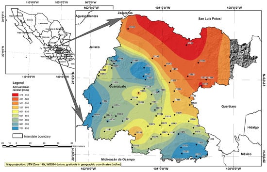
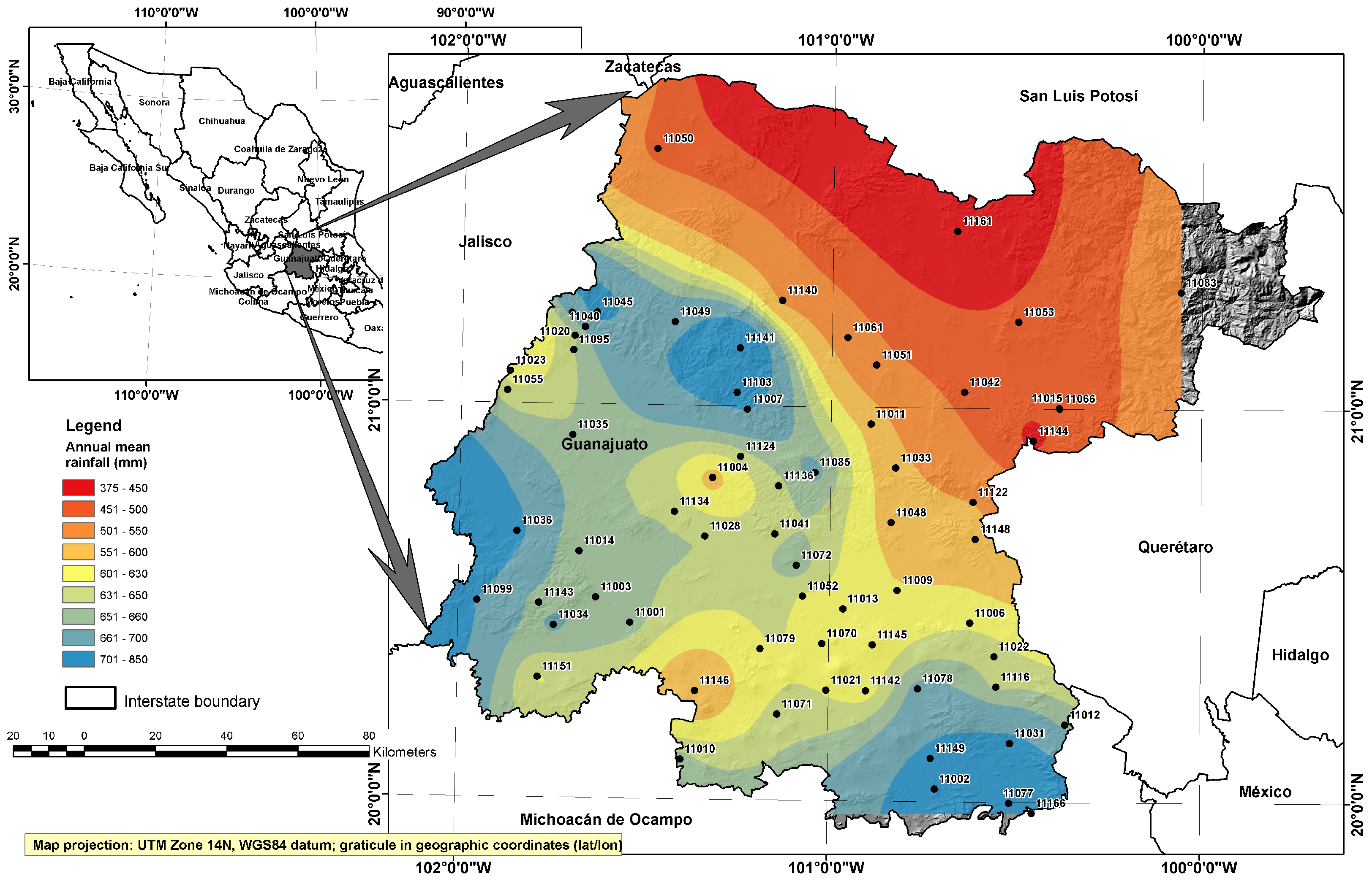
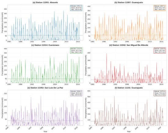
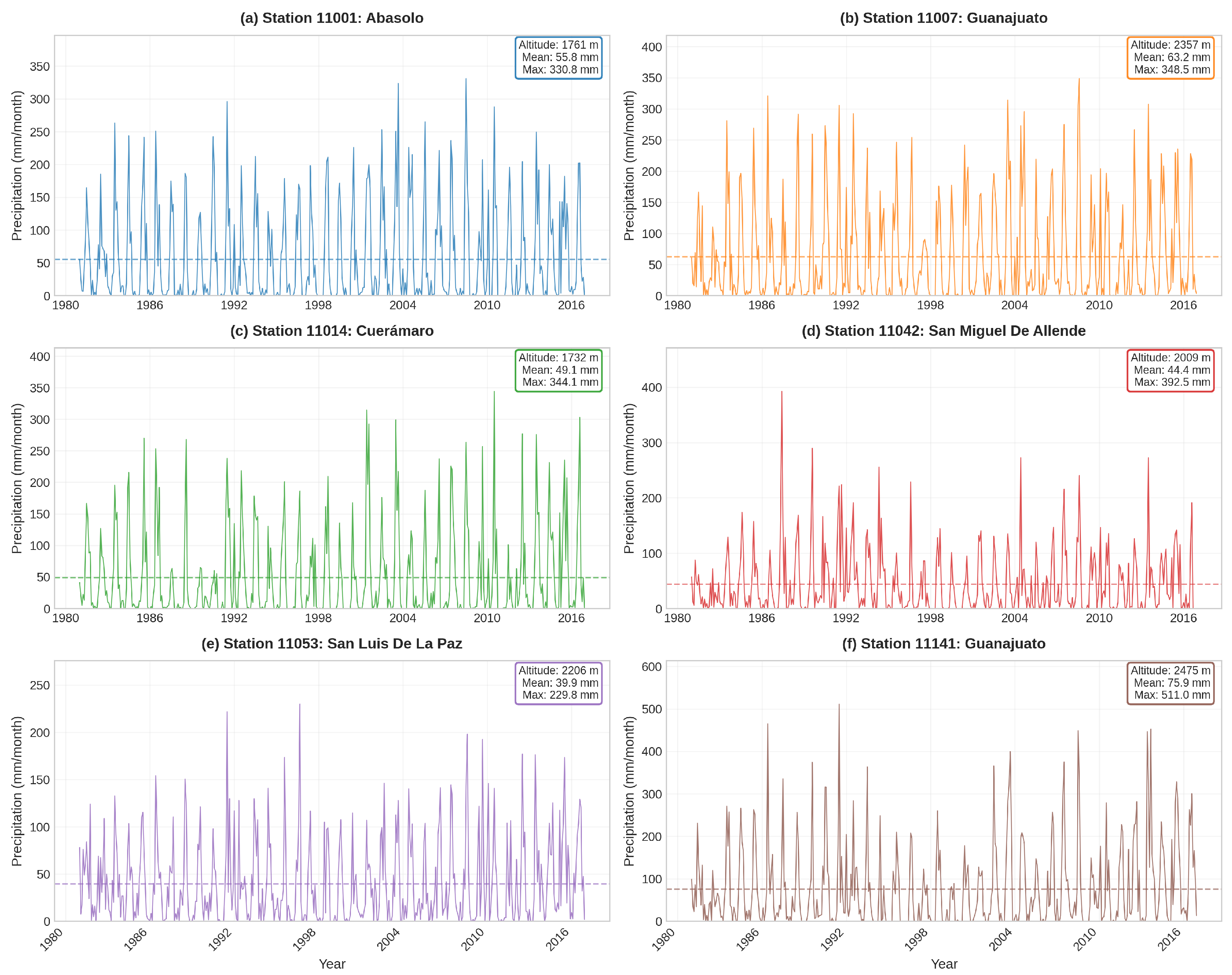
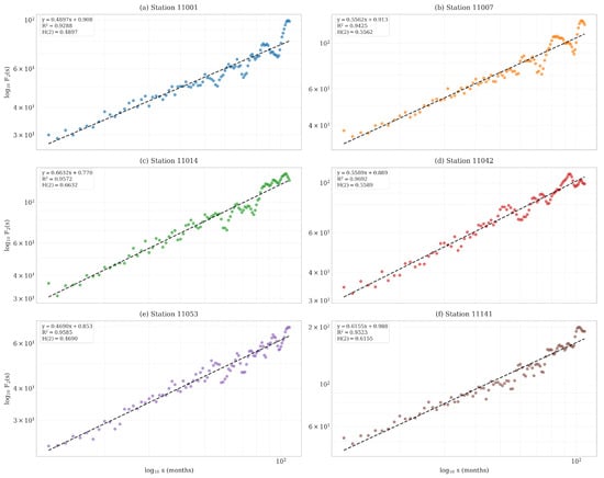
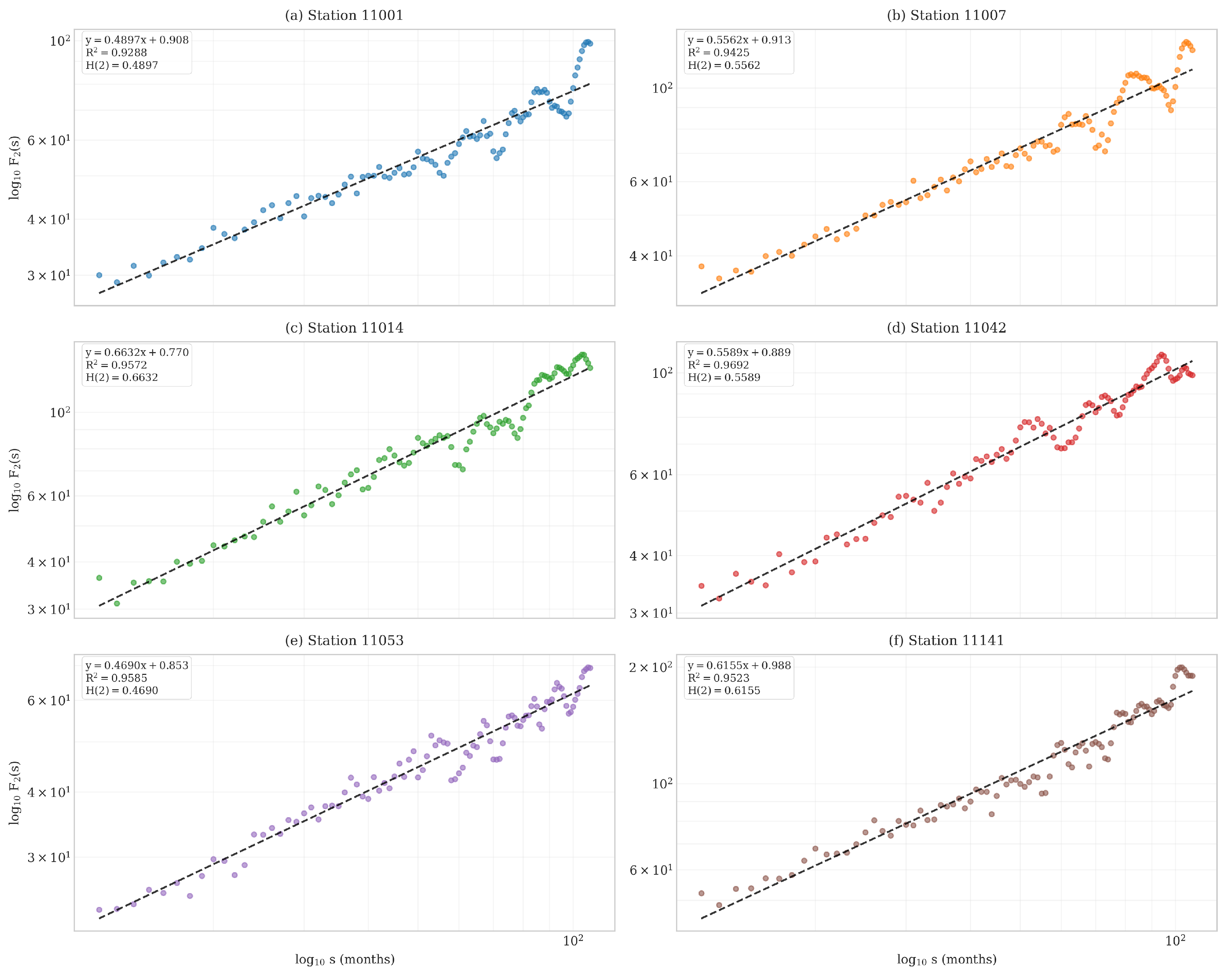
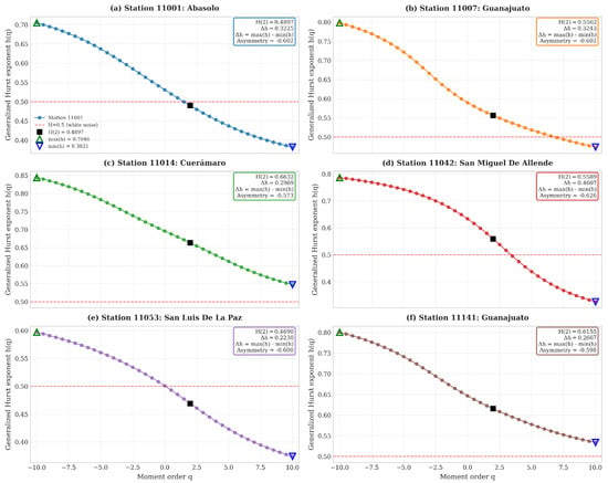
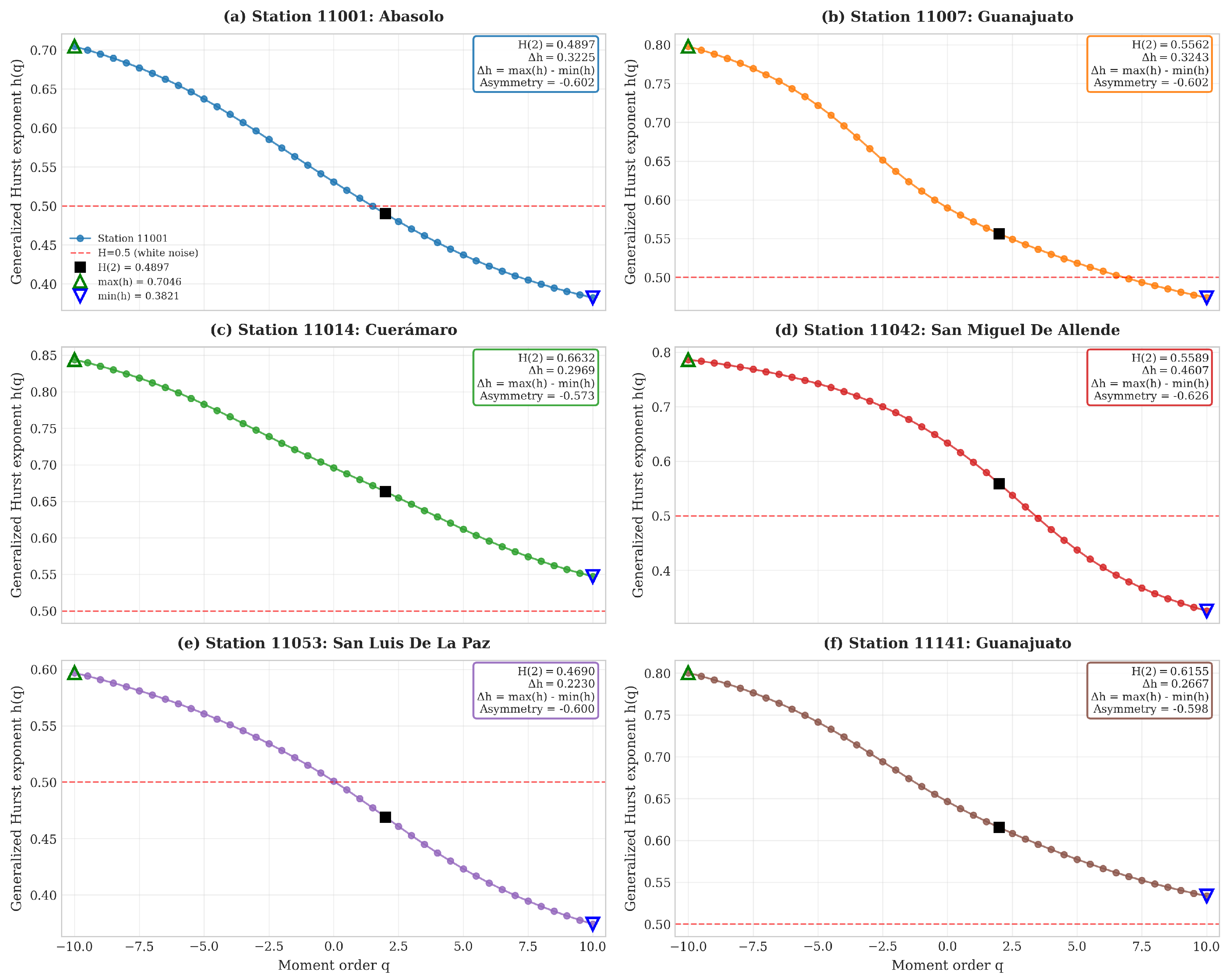
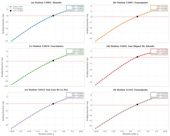
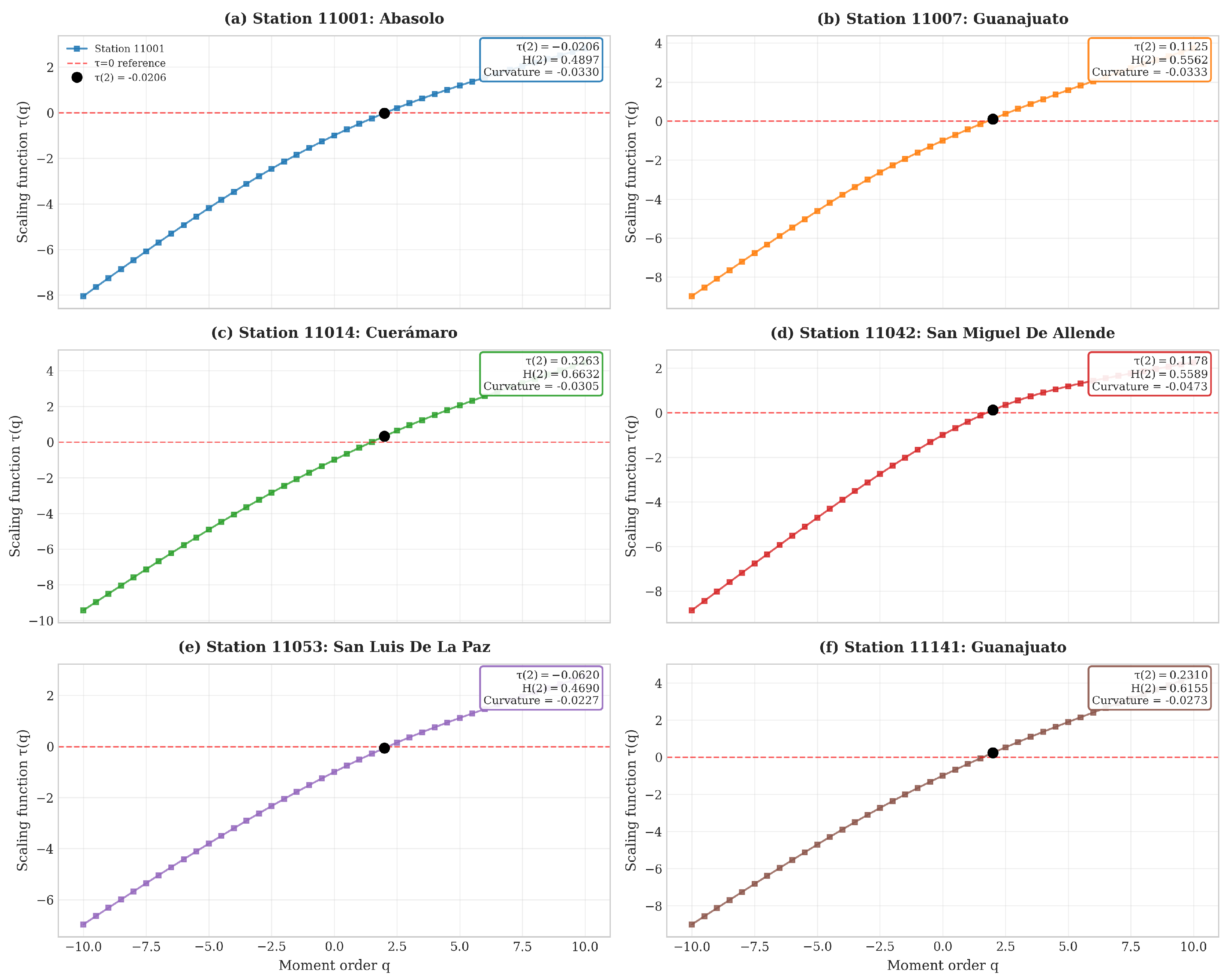
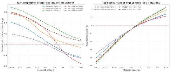
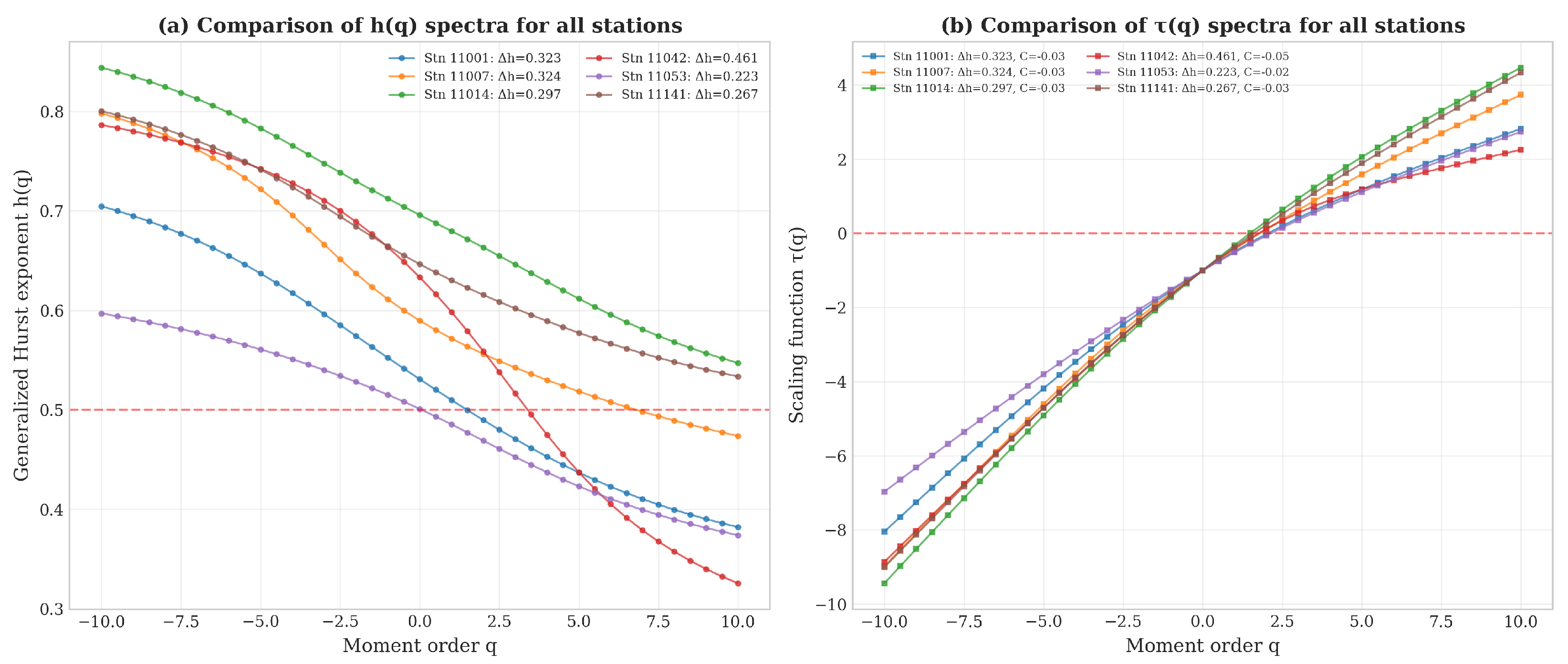
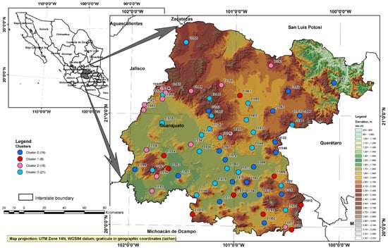
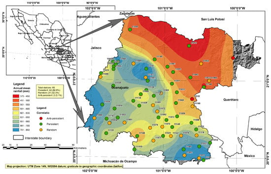
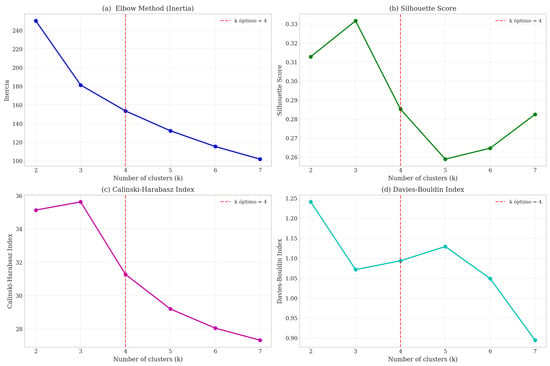
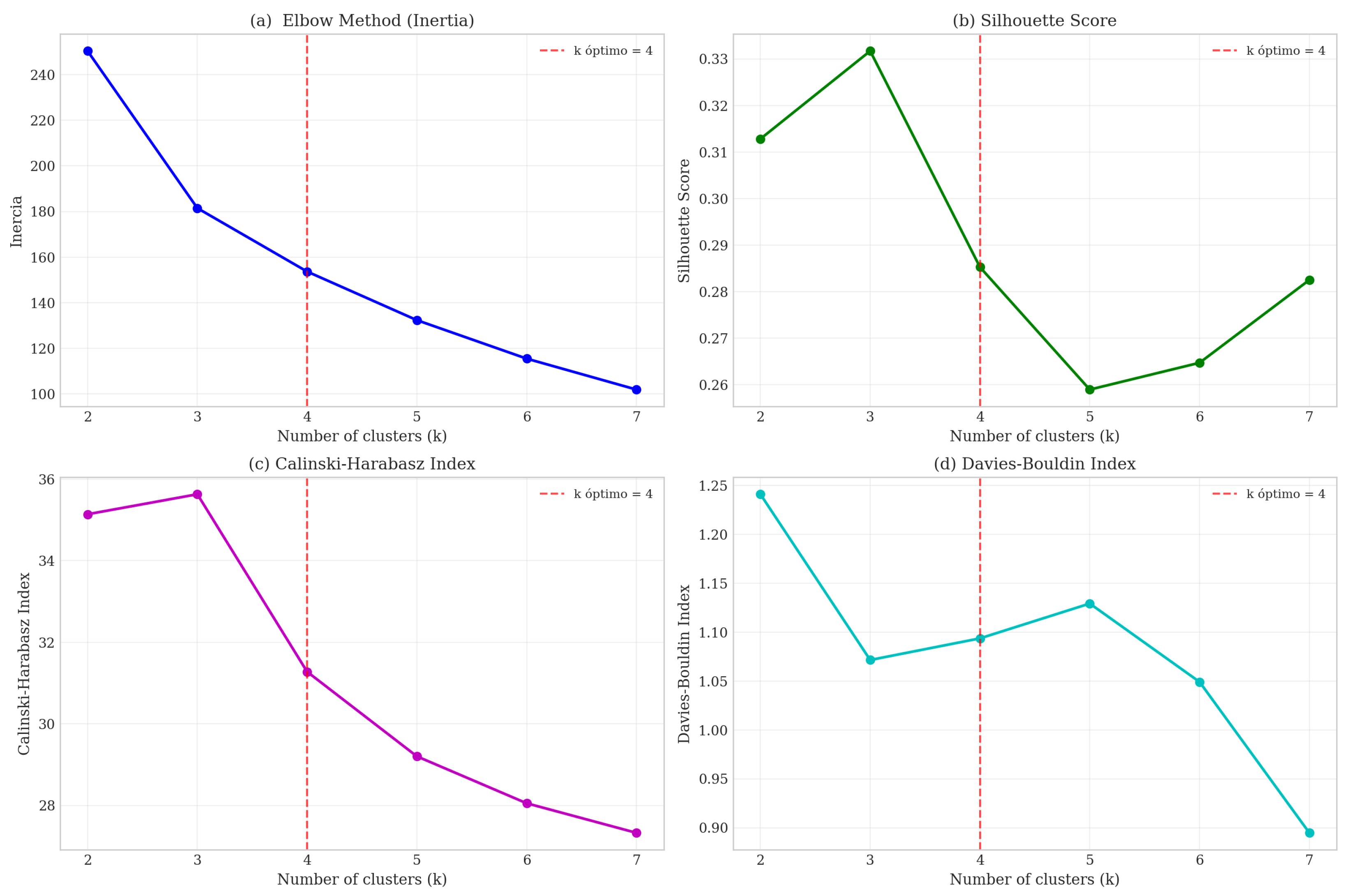

Disclaimer/Publisher’s Note: The statements, opinions and data contained in all publications are solely those of the individual author(s) and contributor(s) and not of MDPI and/or the editor(s). MDPI and/or the editor(s) disclaim responsibility for any injury to people or property resulting from any ideas, methods, instructions or products referred to in the content. |
© 2026 by the authors. Licensee MDPI, Basel, Switzerland. This article is an open access article distributed under the terms and conditions of the Creative Commons Attribution (CC BY) license.