Analysis of Driving Factors and Trend Prediction of Groundwater Levels in the West Liao River Basin Based on the STL-LSTM Model

Abstract

In the ecologically fragile West Liao River Basin, characterizing groundwater dynamics is crucial for sustainable water management. Using 2000–2016 groundwater level data, this study applies Seasonal-Trend decomposition using Loess (STL) and change-point detection to analyse trends. Driving factors are quantified via random forest combined with SHapley Additive exPlanations (SHAP) analysis, and a novel STL–Long Short-Term Memory (STL-LSTM) hybrid model is developed for forecasting. Key findings include: (1) Groundwater levels declined persistently, with a significant change point in 2009. The post-2009 decline rate accelerated to −0.749 m/yr, a 55.7% increase. (2) Statistical attribution reveals that soil moisture (43.5%) and climatic factors (29.0%) are the primary predictors of groundwater variability. The dominance of soil moisture highlights the key role of agricultural irrigation, which strongly modifies soil water dynamics during the growing season. (3) The STL-LSTM model achieves optimal predictive performance (R² = 0.8805, RMSE = 0.7081 m), demonstrating enhanced accuracy for non-stationary sequences. This integrated framework combines trend diagnosis, driver interpretation, and hybrid modelling, offering scientific support for precise groundwater management in semi-arid agricultural basins.

1. Introduction

Groundwater is a vital strategic freshwater resource that supports agricultural production, domestic and industrial water supply, and the stability of riverine and terrestrial ecosystems, especially in arid and semiarid regions where surface water is relatively scarce [1,2]. Under the combined pressures of increasing climate variability and intensifying human water use, groundwater depletion has become a major global resource and environmental issue, posing persistent threats to water security, food production, and ecological sustainability [3,4]. In northern China, this problem is particularly severe in the agro-pastoral ecotone, where limited precipitation, strong evaporation, and a high dependence on agricultural irrigation further increase the vulnerability of groundwater systems [5,6]. The West Liao River Basin (WLRB), located in the transitional zone from semi-humid to semiarid climate in northeastern China, is a typical ecologically fragile basin [7]. The basin receives only about 338.8–406.7 mm of annual precipitation, more than 75% of which is concentrated between June and September, whereas annual evaporation reaches 1700–2000 mm, indicating inherently limited water availability. Meanwhile, the West Liao River Plain is one of China’s important grain-producing regions, where agricultural irrigation accounts for 75–88.9% of total regional water consumption [8]. Long-term intensive groundwater abstraction has led to a pronounced imbalance between recharge and discharge, resulting in continuous groundwater decline, reduced surface runoff, and increasing hydrological and ecological stress [9]. Therefore, the WLRB provides a representative setting for investigating groundwater level evolution and its driving mechanisms under the combined influences of climate change and human activities [10].

In recent years, groundwater changes and their driving factors have attracted increasing attention, providing an important basis for understanding the evolution of regional water resources [11]. Existing studies have mainly relied on groundwater monitoring records, Gravity Recovery and Climate Experiment (GRACE) satellite observations, multisource remote sensing products, and hydrometeorological data to analyze long-term trends, spatial heterogeneity, and stage-wise changes in groundwater levels or groundwater storage [12]. These studies indicate that groundwater decline has become a widespread phenomenon in many arid and semiarid regions [13]. In the WLRB, previous research based on GRACE and in situ observations has shown that groundwater storage has continuously decreased, and that persistent drought since the late 1990s, together with excessive groundwater abstraction, has accelerated regional groundwater depletion [14]. Studies focusing on the WLRB and the broader agro-pastoral ecotone of northern China have further demonstrated that terrestrial water storage in this region has remained persistently deficient and is closely associated with climate variability, vegetation change, and human activities [7]. At the same time, research on the driving mechanisms of groundwater change has continued to deepen [15]. Existing evidence suggests that both natural and anthropogenic factors, including climate variability, vegetation dynamics, land use change, irrigation expansion, and groundwater pumping, jointly shape groundwater evolution [16]. In recent years, machine learning methods such as random forests, support vector machines, and neural networks have also been increasingly applied to groundwater-related analysis and prediction, providing new technical pathways for identifying nonlinear responses in complex systems [17,18]. In addition, studies using SHapley Additive exPlanations (SHAP) have shown that the impacts of climatic and human-related factors on groundwater are often not independent, but instead arise through coupled interactions among multiple variables [19]. However, most existing studies still remain limited to whole-period attribution, static importance ranking, or broad stage-wise comparisons, and there is still a lack of dynamic understanding of whether driving mechanisms shift across critical transition periods [20]. Therefore, there is a clear need to better integrate groundwater change diagnostics with driver attribution so as to more systematically reveal the dynamic mechanisms underlying groundwater evolution [21].

Compared with groundwater change diagnostics and driver attribution, groundwater level prediction places greater emphasis on accurately characterizing complex temporal features [22]. Groundwater level series usually contain long-term trends, seasonal fluctuations, and irregular disturbances simultaneously, while also being influenced by precipitation, evapotranspiration, groundwater abstraction, irrigation activities, and hydrogeological conditions [23,24]. Consequently, such series often exhibit pronounced nonlinearity, nonstationarity, and multiscale variation [25]. Traditional physically based models such as MODFLOW can describe groundwater evolution from a mechanistic perspective, but they generally require detailed information on aquifer structure, boundary conditions, and model parameters, and often face high data demands and computational costs in parameter calibration and real-time prediction [26,27]. In recent years, with the rapid development of data-driven approaches, Long Short-Term Memory (LSTM), Transformer, and related deep learning models have gradually been applied to groundwater level prediction, showing clear advantages in capturing temporal dependencies and improving forecasting accuracy [28]. However, most existing studies still model raw groundwater level series directly, making it difficult to effectively distinguish long-term trends, seasonal cycles, and random fluctuations at different scales [29]. In addition, the understanding gained from earlier change diagnostics and driver attribution has rarely been incorporated into subsequent forecasting frameworks [30]. Previous studies have shown that, for nonstationary series, decomposing the original sequence into different components and then modeling and reconstructing each component separately can help reduce the adverse effects of nonstationarity on predictive performance and improve the representation of complex dynamic processes [28]. Therefore, for a typical region such as the WLRB, where groundwater level variations are strongly affected by both climate change and intensive human activities, a decomposition-based prediction strategy is needed [31]. On this basis, integrating Seasonal-Trend decomposition using Loess (STL) with deep learning models may provide more robust methodological support for groundwater level prediction.

Based on the above considerations, this study takes the WLRB as the study area and systematically investigates groundwater level changes during 2000–2016 by integrating STL decomposition, change-point detection, random forest and SHAP attribution analysis, and deep learning prediction methods. This study aims to address two major limitations in current research: the insufficient integration between groundwater evolution diagnostics and dynamic attribution of driving mechanisms, and the relative lack of high-accuracy forecasting frameworks for nonstationary groundwater level series. We propose that groundwater level evolution in the WLRB exhibits clear stage-dependent characteristics, and that the effects of major driving factors may differ before and after critical transition points. Furthermore, for nonstationary groundwater level series, the introduction of STL decomposition is expected to enhance the ability of deep learning models to characterize complex variation processes. Specifically, this study aims to: (1) identify the spatiotemporal evolution characteristics of groundwater levels in the WLRB and detect their key transition points; (2) analyze the dominant driving factors and their changing influences before and after the transition, with particular emphasis on the impacts of human activities; and (3) compare the applicability of different deep learning models for groundwater level prediction and develop an integrated analytical framework linking evolution diagnostics, driver attribution, and trend forecasting. Through these efforts, this study seeks to deepen understanding of groundwater system responses in the WLRB from the perspectives of evolutionary pattern identification, driving mechanism quantification, and nonstationary time-series prediction, thereby providing a scientific basis for regional groundwater resource management.

2. Materials and Methods

2.1. Study Area

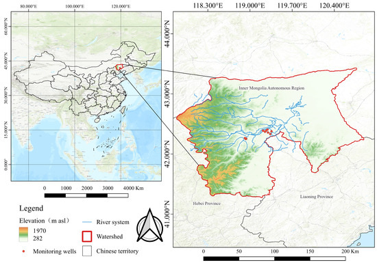
The West Liao River Basin is located in the southwestern part of Northeast China (116°32′ E–124°29′ E, 41°08′ N–45°22′ N). The total basin area is approximately 138,300 km², comprising about 51,600 km² of plains and 83,600 km² of mountainous and hilly terrain. The basin has a temperate continental monsoon climate and lies in the transition zone between semi-humid and semi-arid regions, with limited water availability due to high evaporative demand relative to precipitation [32].

Hydrogeologically, the plain area is characterised by pore water in loose rock formations [33]. The West Liao River Plain is situated within the ‘Golden Corn Belt’ and serves as a key national grain production base [34]. Agricultural irrigation is the dominant water user, and due to intensive extraction, groundwater pumping has now surged to four times the level recorded in 1980 [35].

2.2. Data Sources

This study collected multi-source spatiotemporal data spanning 204 months, from January 2000 to December 2016, covering groundwater depth monitoring, meteorological data, vegetation indices, soil moisture, and agricultural statistics. All data were standardised to a monthly scale for analysis; details regarding data types, spatial resolution, and sources are provided in Table 1.

Table 1. Data Source Description.

Data	Spatial Resolution	Data Source
Groundwater Level	Point Data	Monitoring Wells Actual Measurement Data
Air Temperature and Precipitation	0.25° × 0.25° Grid Cells	National Centres for Environmental Information (NCEI), National Oceanic and Atmospheric Administration (NOAA)
Evapotranspiration (EVAP)	0.25° × 0.25° Grid Cells	Global Land Surface Assimilation System jointly developed by NASA Goddard Space Flight Centre (GSFC) and the National Centres for Environmental Prediction (NCEP)
Normalised Difference Vegetation Index (NDVI)	0.25° × 0.25° Grid Cells	NASA Earth Observing (NEO) website
Soil moisture at 7 cm, soil moisture at 28 cm	0.25° × 0.25° Grid Cells	Global Land Surface Assimilation System jointly developed by NASA Goddard Space Flight Centre (GSFC) and the National Centres for Environmental Prediction (NCEP)
Agricultural cropland area	Panel Data	Local Statistics Bureaus, Local Statistical Yearbooks

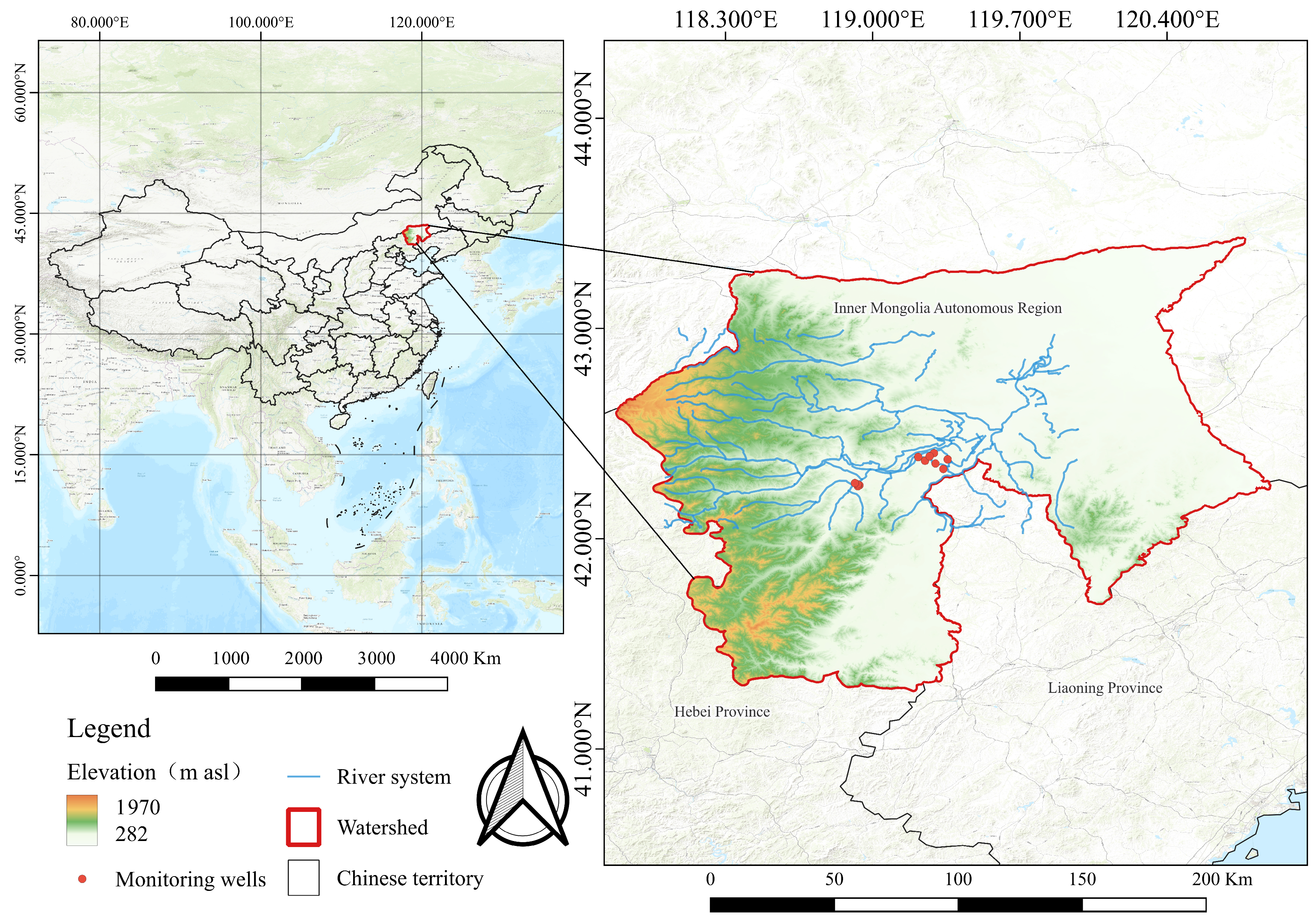
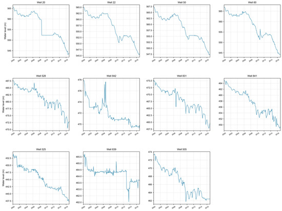
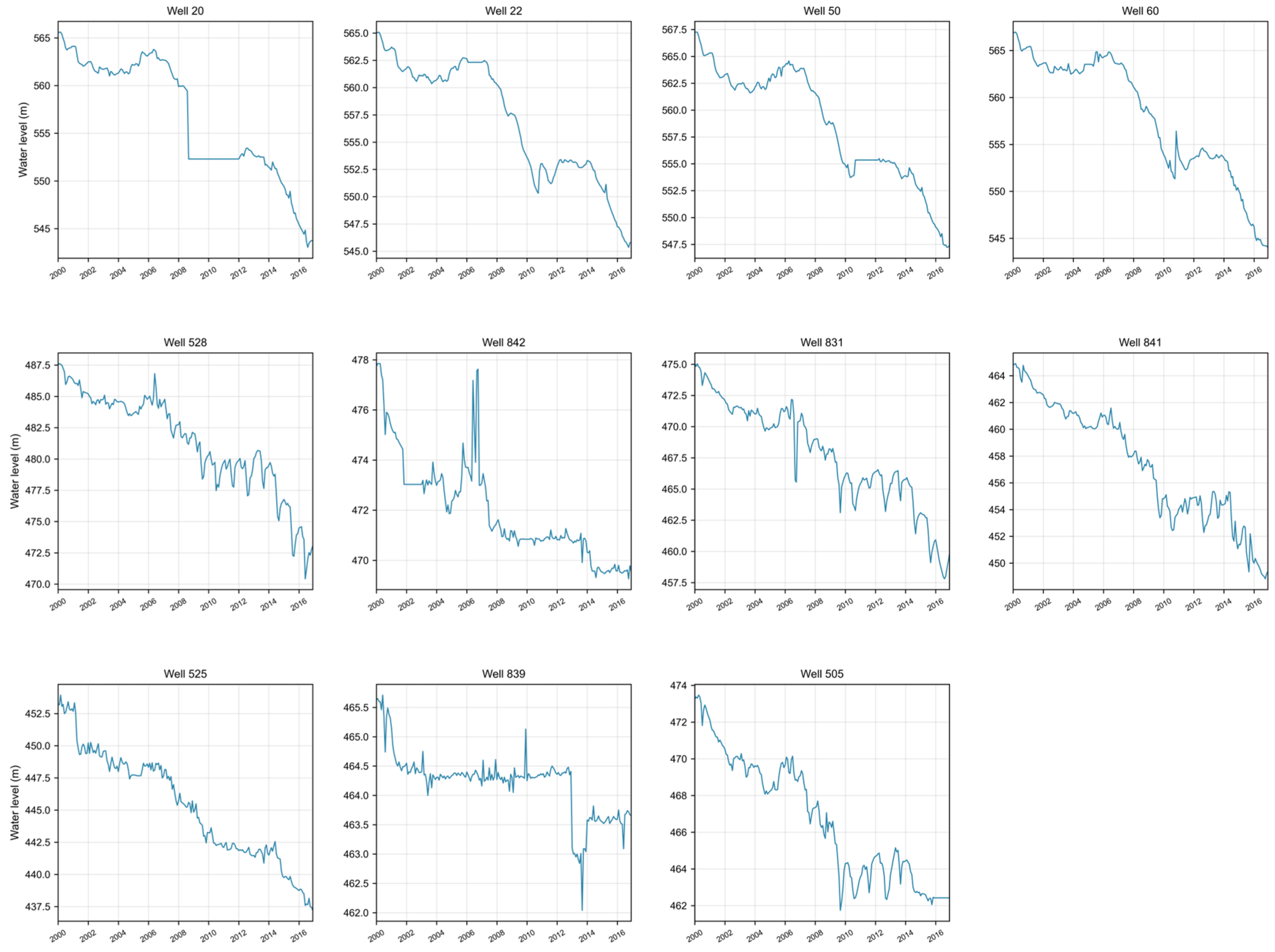
The groundwater depth monitoring network comprises 11 wells (Figure 1). Among these, Wells 20, 22, 50, and 60 are located in the western part of the watershed and serve as urban monitoring wells; the remaining seven wells (528, 842, 831, 841, 525, 839, and 505) are distributed across the central and eastern regions and function as regional monitoring wells. Figure 2 shows the raw time series of groundwater levels for each well during the study period (2000–2016), reflecting a sustained downward trend and spatial heterogeneity.

Figure 1. Location Map of the West Liao River Basin.

Figure 2. Raw groundwater level time series from 11 monitoring wells (2000–2016).

2.3. Analysis of Spatiotemporal Characteristics and Driving Factors of Groundwater Dynamics

2.3.1. Geostatistical Analysis

To systematically reveal the spatial patterns of groundwater changes in the West Liao River Basin, this study employed a multilevel geostatistical approach. First, monthly variations in water levels at each monitoring well relative to the January 2000 baseline were calculated to eliminate initial differences in water levels between sites. Spatial dispersion was assessed using the coefficient of variation, while spatial autocorrelation was tested with the global Moran’s I index [36].

The semivariogram was employed to quantify the spatial structure of groundwater variations, expressed in Equation (1):

$$\widehat{\gamma }(h)={\displaystyle \frac{1}{2N(h)}}{\displaystyle \sum _{i=1}^{N(h)}{\left[Z(x_i)-Z(x_i+h)\right]}^2}$$

(1)

where $Z(x_i)$ and $Z(x_i+h)$ represent the observed values at positions $x_i$ and $x_i+h$; $h$ denotes the lag distance; $N(h)$ is the number of samples at distance $h$.

Analysis indicates that the annual groundwater variation exhibits significant spatial clustering (Moran’s $I=0.083$, $p<0.001$), but the spatial autocorrelation of the multi-year average variation is not significant (Moran’s $I=0.083$, $p<0.062$). Water level change sequences across stations exhibited high synchrony (mean correlation coefficient 0.86), supporting the use of spatially averaged time series to characterize the regional system as a whole. Consequently, subsequent time-series analyses were conducted based on the spatially averaged water level change sequences.

2.3.2. Time Series Decomposition

To effectively separate long-term trends, seasonal cycles, and random fluctuations from raw groundwater level sequences, this study employed the Seasonal-Trend decomposition procedure based on Loess (STL) to decompose regional average water level sequences [37]. The STL method exhibits strong robustness against non-stationary time series and outliers. Its additive decomposition model can be expressed in Equation (2):

$$Y_t=T_t+S_t+R_t$$

(2)

Among these, $Y_t$ represents the original observation at time $t$, $T_t$ is the trend component, $S_t$ is the seasonal component, and $R_t$ is the residual component. STL decomposition parameter settings for the 17-month monthly series: The seasonal component period is fixed at 12 months to reflect the annual rhythm of agricultural irrigation, while the seasonal component smoothing window is set to 13 months to capture stable periodic patterns.

2.3.3. Breakpoint Analysis

To identify the phased evolution characteristics of the groundwater system in the West Liao River Basin, this study employed a combined test method integrating the Sliding t-test with the Mann–Kendall (M-K) trend test to perform breakpoint analysis on regional spatially averaged relative water level sequences [38]. The sliding t-test examines point-by-point differences in the means of preceding and subsequent sub-sequences by setting a sliding window (this study employed an adaptive window $w=\max (3,\min (7,⌊N/3⌋))$. For a water level sequence $\left\{x_i\right\}$ of length $N$, the $T$ statistic at position $i$ is calculated using Equation (3):

$$t_i={\displaystyle \frac{{\overline{X}}_1-{\overline{X}}_2}{S_p\sqrt{\frac{2}{w}}}}$$

(3)

where ${\overline{X}}_1$ and ${\overline{X}}_1$ denote the means of the preceding and subsequent sub-sequences, respectively, and $S_p$ is the pooled standard deviation. A potential mutation point is identified when the two-tailed test yields $p<0.01$. The Mann-Kendall trend test is used to verify the significance of trends in the overall data and each segment $(\alpha =0.05)$. Its statistic $S$ is defined in Equation (4):

$$S={\displaystyle \sum _{i=1}^{N-1}{\displaystyle \sum _{j=i+1}^N\mathrm{sgn}}}(x_j-x_i)$$

(4)

The rate of trend change is estimated by Sen’s slope: $\beta =\mathrm{median}\left({\displaystyle \frac{x_j-x_i}{j-i}}\right)$. To enhance the reliability of results, a minimum segmentation length of 5 years was set, with a minimum interval of 3 years between transition points. Post-processing algorithms were employed to select transition points exhibiting the highest statistical significance and clear hydrological relevance. This method effectively identifies phased evolution characteristics of groundwater systems, providing a scientific basis for subsequent analysis of driving mechanisms.

2.3.4. Analysis of Driving Mechanisms

To quantify the nonlinear driving contributions of various natural and anthropogenic factors to groundwater levels, this study employed a Random Forest ensemble learning model combined with the SHAP (SHapley Additive Explanations) game theory interpretation framework for attribution analysis [39,40].

Random forests effectively handle complex nonlinear relationships among high-dimensional features by constructing multiple decision trees and integrating their predictions. Its core principle can be expressed in Equation (5):

$$\widehat{y}={\displaystyle \frac{1}{B}}{\displaystyle \sum _{b=1}^B{T}_b}(x)$$

(5)

After training the random forest model, SHAP values are employed for attribution analysis. SHAP value ${\varphi }_i$, based on cooperative game theory, provides a unified and fair allocation scheme for each feature $i$ contribution to a single prediction, as defined in Equation (6):

$${\varphi }_i(f_x)={\displaystyle \sum _{S\subseteq N\setminus \left\{i\right\}}\frac{\left|S\right|!(|N|-|S|-1)!}{\left|N\right|!}}\left[f_x(S\cup \{i\})-f_x(S)\right]$$

(6)

Here, $N$ is the set of all features, $S$ is a subset of features, and $f_x(S)$ is the model prediction value using feature subset $S$.

To ensure the reliability and interpretability of attribution results, this study initially screened candidate features using the mutual information method, subsequently excluding variables exhibiting significant multicollinearity (variance inflation factor $VIF>5$) or overlapping physical meanings. The final input features include: air temperature, precipitation, evapotranspiration, NDVI, surface soil moisture (7 cm), deep soil moisture (28 cm), and seasonal sine and cosine components, totaling eight variables. These features comprehensively reflect the direct impacts of climate, vegetation, soil moisture, and seasonal cycles on the groundwater system.

Model training employed random forest regression $(\mathrm{n}\_\mathrm{estimators} = 200, \max \_\mathrm{depth} = 8, \min \_\mathrm{samples}\_\mathrm{leaf} = 5)$. Based on breakpoint analysis results (2009), the study period was further divided into an early phase (2000–2008) and a late phase (2009–2016). SHAP values were calculated for each phase to reveal dynamic changes in driving factors.

2.4. Groundwater Level Prediction Model Development and Performance Comparison

To enhance prediction capabilities for non-stationary groundwater sequences, this study developed and compared four deep learning models: LSTM, Transformer, STL-LSTM, and STL-Transformer. All models utilised a unified multi-source feature set. Training sequences were constructed using a sliding window approach with a window length of 5 months. Data were divided into training (143 samples) and testing (61 samples) sets in a 7:3 ratio based on chronological order. To ensure transparency and reproducibility of the forecasting framework, Table 2 summarizes the key technical parameters used in this study.

Table 2. Summary of key forecasting parameters.

Parameter	Value
Temporal resolution	Monthly
Time series length	204 months (2000–2016)
Target variable	Relative change (Δh)
Historical window size	5 months
Prediction horizon	1 month (single-step)
Forecasting type	Sequence-to-single
Training samples	143 (70%)
Testing samples	61 (30%)

2.4.1. Data Preparation and Input Variable Construction

The regional average relative water level change sequence $(\Delta h)$, defined in Section 2.3.1, was used as the prediction target. An input variable set comprising 24 variables (Table 3) was constructed, covering climatic factors, vegetation-soil factors, human activity indicators, and temporal encoding. Before constructing the training dataset based on the aforementioned 5-month sliding window, all variables were normalised using Z-score standardization.

Table 3. List of Input Variables for Groundwater Level Prediction Model. Note: The weighting of the irrigation index is set according to agricultural activity patterns, with values ranging from 0.10 to 0.30 during the irrigation season (March to September) and from 0.02 to 0.05 during the non-irrigation season.

Feature Category	Specific Variables	Quantity	Description
Climate Factors	Air Temperature, Precipitation, Evapotranspiration	3	Raw Values
	Air Temperature/Precipitation/Evapotranspiration_lag1–3	9	1st to 3rd Order Lags—Capturing Dynamic Climate Memory
Vegetation & Soil Factors	NDVI, Soil Moisture (7 cm/28 cm)	3	Raw Values—Direct Indicators of Surface Dynamics
	NDVI/Soil Moisture_lag1–3	9	Lagged Effects—Uncovering Delayed Responses in Eco-Hydrology
Human Activity Indicators	Cropland Area	1	Hectares—Scaling Agricultural Footprint
	Irrigation Index	1	Cropland Area × Monthly Weight—Quantifying Seasonal Irrigation Impact
Time Series Encoding	month_sin, month_cos	2	Monthly Sine-Cosine Encoding—Embedding Cyclical Temporal Patterns

2.4.2. Benchmark Prediction Model

The LSTM model employs a long short-term memory network architecture [41]. This model employs a two-layer LSTM architecture with 48 hidden units and a dropout rate of 0.1; these parameters were optimised through grid search. It performs end-to-end temporal modelling and prediction directly on the raw regional average water level change sequence.

The Transformer model employs an encoder architecture based on self-attention mechanisms [42]. The model configuration includes four attention heads with a feature dimension of 64 and uses sine-cosine position encoding. This model also directly predicts the raw water level sequence, leveraging its self-attention mechanism to capture global dependencies within the sequence.

2.4.3. Ensemble Model Construction

To enhance modelling capabilities for non-stationary sequences, this study proposes two types of ensemble prediction models based on STL decomposition. Their core workflow follows the “decomposition-prediction-reconstruction” steps:

(1)

Decomposition: STL decomposition is applied to the entire time series to extract trend, seasonal, and residual components. These components serve as the prediction targets for three independent submodels, rather than as input features. The dataset is then split chronologically into a training set (70%) and a test set (30%).

(2)

Forecasting: After decomposition, dedicated sub-models are established for each sub-sequence, enabling each model to focus on learning evolutionary patterns at a single scale:

The STL-LSTM model designs differentiated LSTM sub-networks tailored to the distinct characteristics of the three components. Given that trend components change slowly and exhibit long-term dependencies, the forecasting subnetwork employs a two-layer LSTM architecture with 48 hidden units. The seasonal and residual components exhibit relatively complex yet clearly periodic variations. To balance model complexity and overfitting risk, their prediction subnetworks use a single-layer LSTM structure with 32 hidden units. All LSTM subnetworks take the 24-dimensional multi-source features constructed in Section 2.4.1 as input and use the 5-month historical window specified in Table 2.

The STL-Transformer model framework is identical to STL-LSTM, aiming to evaluate the applicability of attention mechanisms in this task. The only difference lies in replacing the prediction subnetworks of each component with Transformer encoders. Each encoder consists of two layers, each with four attention heads. The feature dimension is consistent with the baseline Transformer model, set to 64.

(3)

Reconstruction: The final water level prediction value is obtained by summing the predictions ${\widehat{T}}_t$, ${\widehat{S}}_t$ and ${\widehat{R}}_t$ from the three component models, as shown in Equation (7):

$${\widehat{Y}}_t={\widehat{T}}_t+{\widehat{S}}_t+{\widehat{R}}_t$$

(7)

2.4.4. Hyperparameter Optimization

To ensure optimal model performance, grid search was employed for systematic tuning (Table 4). All models utilised the AdamW optimizer (weight decay 0.005), cosine annealing learning rate scheduling, a batch size of 32, a maximum training epoch of 400, and an early stopping mechanism (patience value 40). The tuning objective was the minimized validation set RMSE.

Table 4. Hyperparameter Grid Search Space.

Model	Hyperparameter	Search Range	Combinations	Optimal Value
LSTM	Hidden Layer Size	[32, 48, 64]	81	48
	Number of Layers	[1, 2, 3]	3	2
	Dropout Rate	[0.1, 0.25, 0.4]	3	0.1
	Learning Rate	[0.001, 0.003, 0.005]	3	0.003
Transformer	Feature Dimension	[32, 48, 64]	189	64
	Number of Attention Heads	[2, 4, 6]	3	4
	Number of Encoder Layers	[1, 2, 3]	3	1
	Dropout Rate	[0.1, 0.25, 0.4]	3	0.1
	Learning Rate	[0.001, 0.003, 0.005]	3	0.003

Prediction performance is evaluated using four metrics: Root Mean Square Error (RMSE), Mean Absolute Error (MAE), Coefficient of Determination (R²), and Mean Absolute Percentage Error (MAPE). All experiments were conducted under identical hardware conditions to ensure comparability of results.

2.4.5. Sensitivity Analysis of Window Length

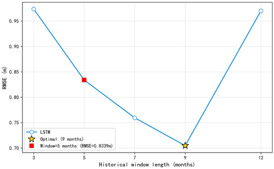
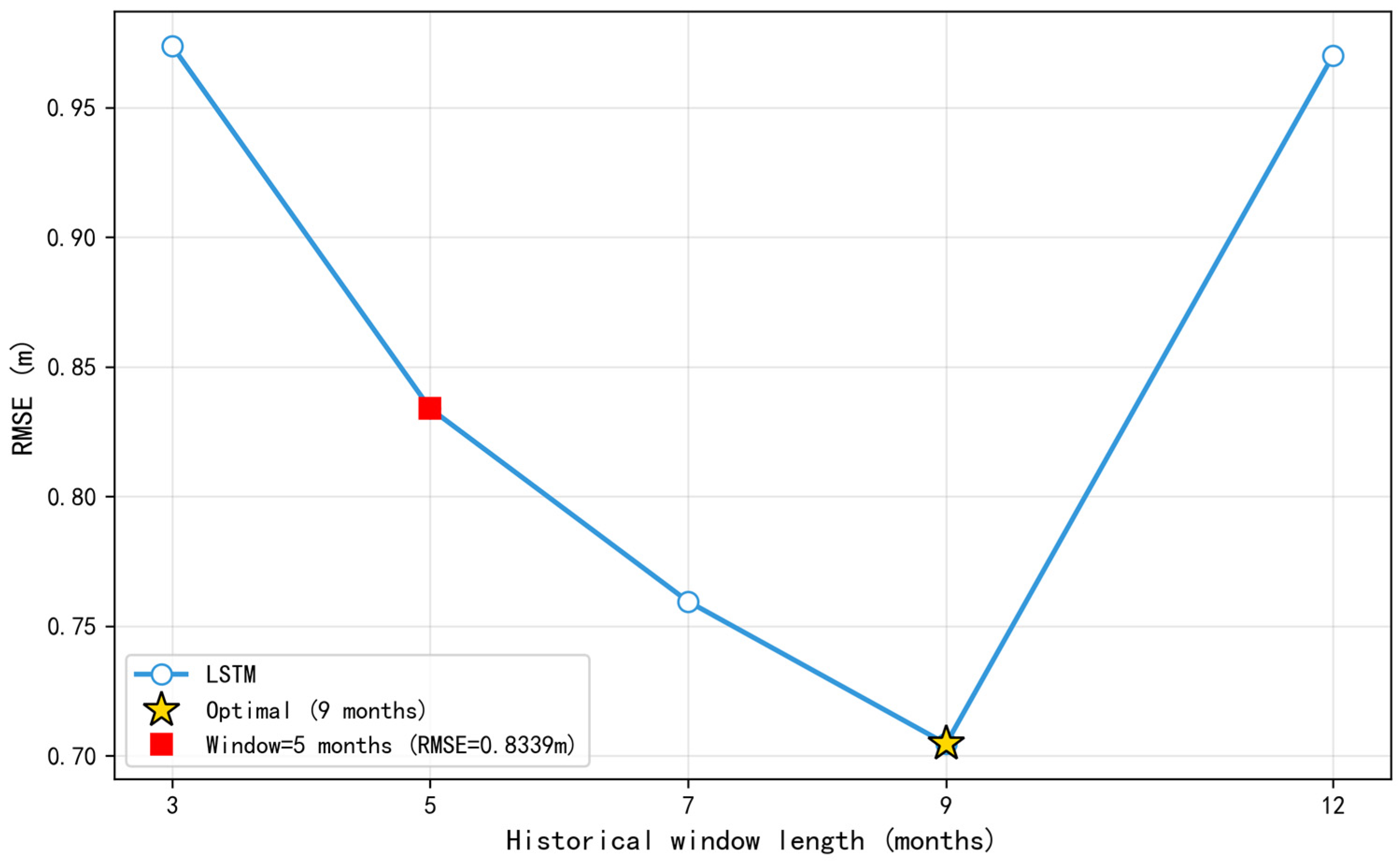
The historical window length is a key hyperparameter that influences the predictive performance of LSTM-based models [43]. To validate the appropriateness of the 5-month window, this study conducted a sensitivity analysis on window length. Using the last 59 samples from the original dataset as the fixed test set, window lengths of 3, 5, 7, 9, and 12 months were set, and LSTM models were trained for each. Their predictive performance (RMSE) on the same test set was then compared to assess the impact of different window lengths on model accuracy.

3. Results and Discussion

3.1. Analysis of Spatiotemporal Evolution Characteristics

3.1.1. Spatial Distribution Pattern

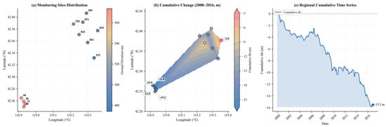
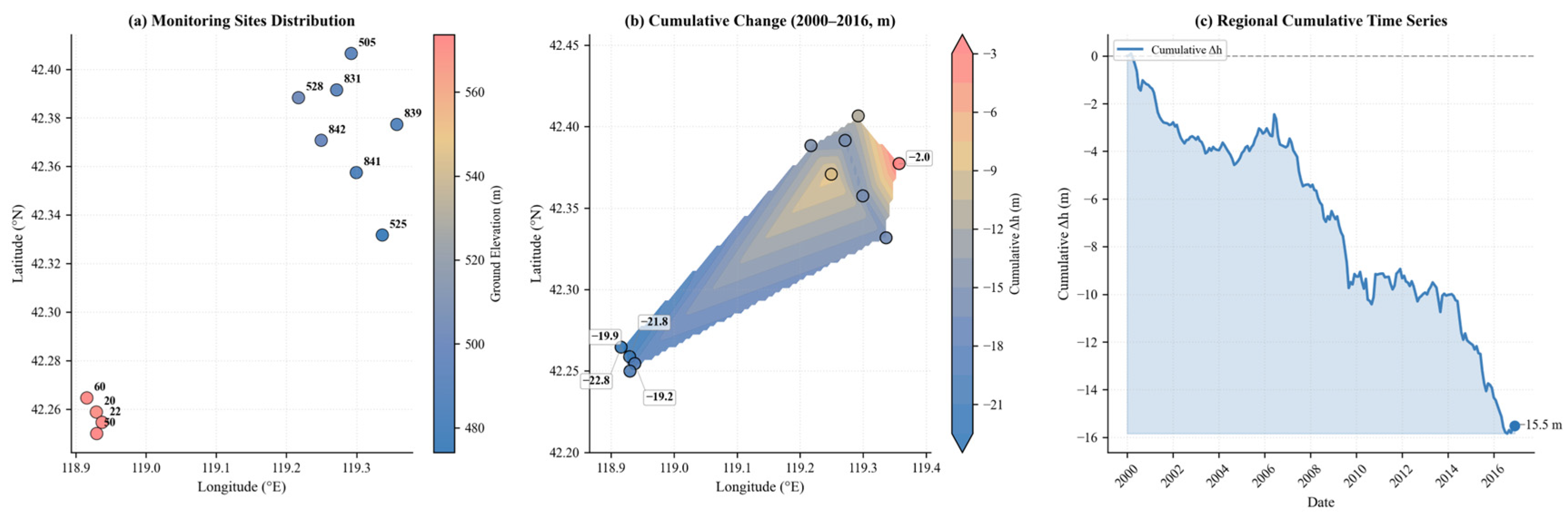
The distribution of the 11 monitoring wells in the West Liao River Basin is shown in Figure 3a; their ground elevations decrease from west to east. Spatial interpolation of the cumulative groundwater level change from January 2000 to December 2016 (Figure 3b) reveals a distinct “west-high, east-low” differentiation: Stations in the western area (20, 22, 50, 60) showed cumulative decline, ranging from −8.20 to −9.14 m over the 17-year period, with annual rates of decline reaching −0.984 to −1.536 m/year; while eastern stations like 839 exhibited the smallest decrease at only −1.42 m, with an annual trend of −0.082 m/year (Table 5). The coefficient of variation for site changes was 30.33%, indicating moderate spatial differentiation.

Figure 3. Spatio-temporal distribution of changes in groundwater depth in the West Liao River Basin (2000–2016). (a) Location of 11 monitoring wells, represented by circles; colours indicate ground elevation. (b) Spatial interpolation of cumulative changes in groundwater depth from January 2000 to December 2016. Western sites (20, 22, 50, 60) experienced the largest declines (>8 m), while the eastern site 839 showed the smallest change (−1.4 m). (c) Regional average cumulative change time series (with January 2000 as the baseline), showing a total decline of 15.27 m by 2016. The gray dashed line indicates the baseline (Δh = 0).

Table 5. Cumulative Decline and Annual Trend of Groundwater Levels at Monitoring Wells.

Site	Cumulative Change 2000–2016 (m)	Annual Change Trend (m/Year)
20	−7.9969	−1.536
22	−8.479	−1.109
50	−8.211	−1.119
60	−9.1444	−1.279
528	−6.2073	−0.747
842	−5.8214	−0.413
831	−7.3052	−0.79
841	−7.3964	−0.858
525	−7.9946	−0.897
839	−1.4181	−0.082
505	−6.2463	−0.678

The regional spatial average sequence (Figure 3c) reveals a continuous decline in groundwater levels from 2000 to 2016, with a cumulative decrease of 15.27 m and an average annual rate of −0.781 m/year (MK test $p < 0.001$).

Spatial autocorrelation analysis further indicates that the annual trend exhibits significant clustering (Moran’s $I = 0.354$, $p < 0.01$), forming a high-rate decline zone centred in the west. Simultaneously, the sequences across stations show high synchrony (mean correlation coefficient 0.86), which weakens with increasing distance. This spatial distribution pattern aligns with the findings of Yan Lingjia et al. [44] regarding the spatial distribution of groundwater overexploitation zones in the western Liaohe Plain. Specifically, parts of Tongliao City and Chifeng City constitute concentrated overexploitation areas, with the western region exhibiting more pronounced overexploitation.

These results indicate that despite spatial variations, the groundwater system in the study area exhibits an overall response to external drivers. Therefore, spatially averaged sequences were selected as regional representatives for subsequent time-series decomposition, abrupt change identification, and driver analysis.

3.1.2. Long-Term Trend and Seasonal Characteristics

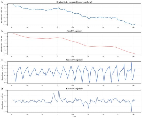
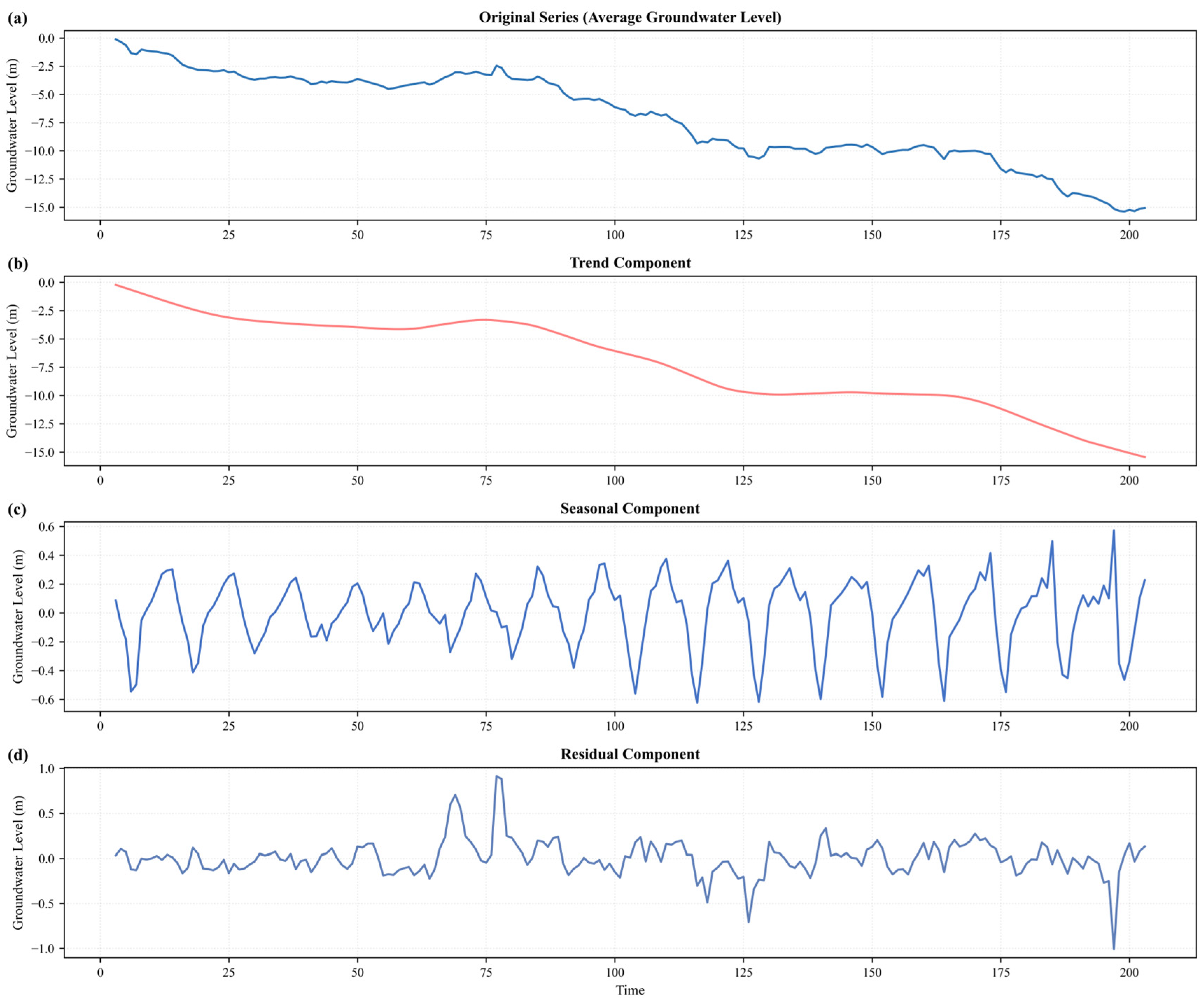
STL decomposition based on relative water level change sequences (Figure 4) indicates that between 2000 and 2016, regional groundwater levels exhibited a pronounced and persistent downward trend, with an average decline of 7.05 m and a maximum drop of 15.38 m. The trend component accounted for 99% of the variation, indicating that intensive human water-use activities are the primary driver of sustained groundwater level evolution in this region, despite limited natural recharge.

Figure 4. STL Time Series Decomposition Results. (a) Original Series; (b) Trend Component; (c) Seasonal Component; (d) Residual Component.

Seasonal analysis reveals a pronounced annual rhythm of “spring rise and autumn fall” in water levels: a relative peak (+0.25 m) occurs in March, while a relative trough (−0.39 m) is reached in September. This pattern aligns closely with the agricultural activity cycle with regional spring irrigation replenishment and concentrated water use during the summer-autumn crop growing season. Research by Chai Zhifu et al. indicates that agricultural irrigation water consumption in the West Liao River Basin reached 4.269 billion m³ in 2022, with Tongliao City and Chifeng City as the primary water-consuming areas [45]. This further confirms the dominant influence of agricultural irrigation on annual groundwater dynamics. However, the amplitude of seasonal fluctuations ($\pm$0.6 m) is significantly smaller than the trend variation (approximately 15 m), indicating that long-term, sustained human water use pressures exert a stronger controlling influence on groundwater dynamics than the modulating effects of natural seasonal variations.

This “spring rise, autumn fall” seasonal pattern closely aligns with the agricultural irrigation cycle in the West Liao River Basin [46]. Spring (March–May) represents the concentrated pre-sowing irrigation period. Combined with snowmelt recharge, groundwater receives some replenishment, leading to a slight rise in water levels. Summer to autumn (June–September) represents the critical growth period for crops like corn, during which irrigation water demand increases significantly. This leads to sustained groundwater extraction, resulting in monthly water level declines that reach their annual low in September. This seasonal fluctuation reflects the cyclical pressure of human irrigation activities on the groundwater system. It confirms that agricultural water use is the key anthropogenic factor regulating the annual dynamics of regional groundwater.

The groundwater drawdown rate of 0.781 m/year in the West Liao River Basin indicates significant regional depletion. This rate is comparable to that of typical international over-exploitation areas, such as the Great Plains of the United States (0.5–1.0 m/year) and California’s Central Valley (0.6–1.0 m/year), higher than that of the Murray-Darling Basin in Australia (0.2–0.4 m/year), but lower than that of the North China Plain (1.0–2.0 m/year) [47,48,49,50]. As in the aforementioned regions, agricultural irrigation is the primary driver. This indicates that the groundwater decline in the West Liao River Basin is not an isolated phenomenon but rather a regional manifestation of irrigation-induced overexploitation in China’s semi-arid agricultural areas.

3.1.3. Change Point Detection

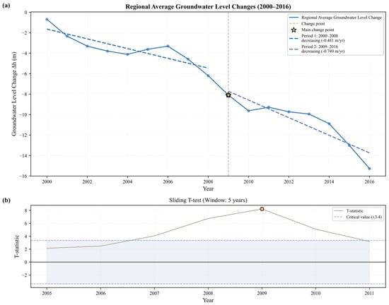
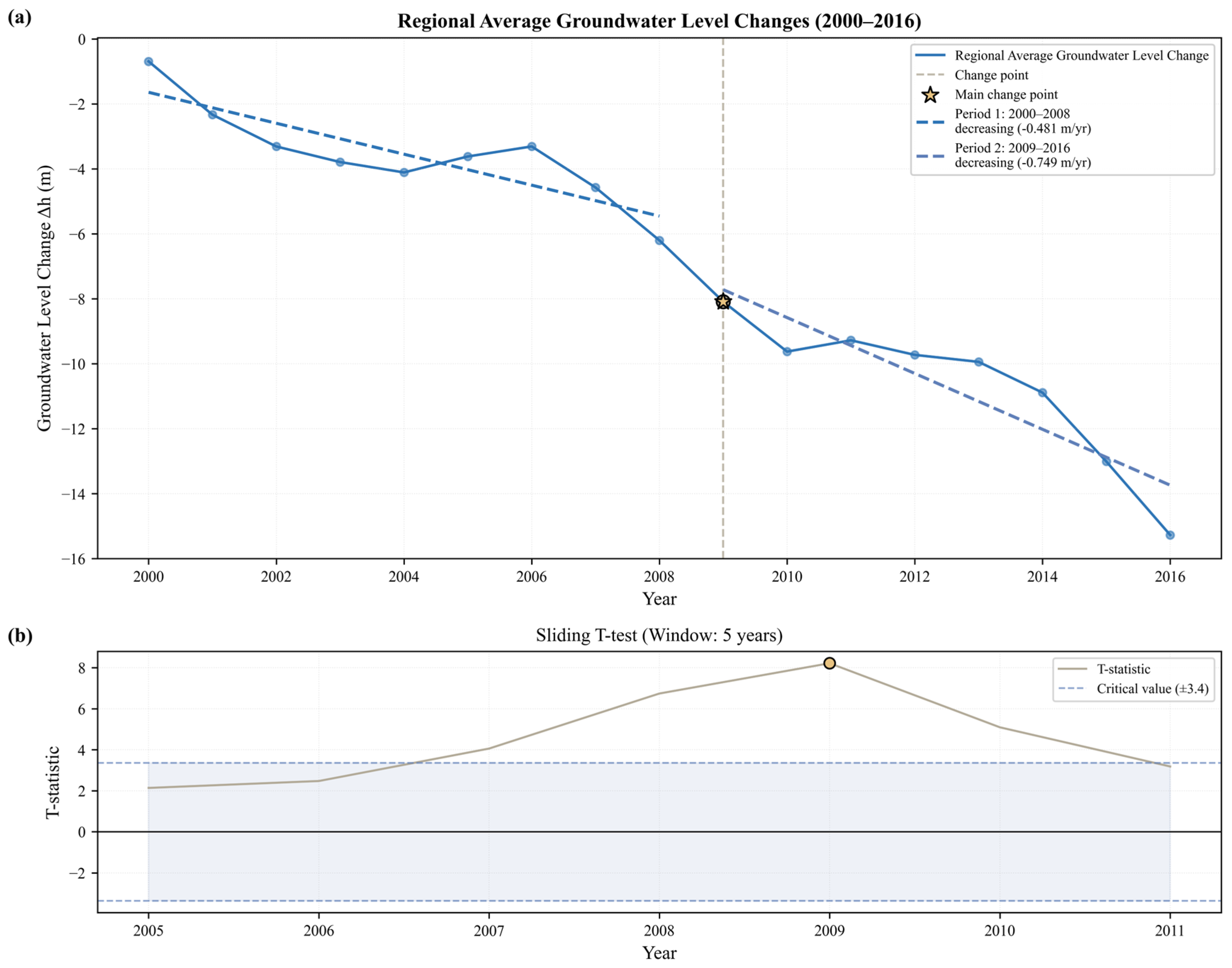
Breakpoint tests were conducted on the regional spatial average groundwater level series of the West Liao River Basin from 2000 to 2016 using the sliding t-test and the combined Mann–Kendall test. Results indicate a statistically significant inflection point detected in 2009 ($p$ < 0.01 for sliding t-test) (Figure 5a). This inflection point divides the entire study period into two phases with markedly different trend characteristics (Table 6): 2000–2008 represented a slow decline phase with a rate of −0.481 m/yr ($p$ = 0.0165); 2009–2016 transitioned to an accelerated decline phase, with the rate increasing significantly to −0.749 m/yr ($p$ = 0.0020), representing a 55.7% increase. The entire sequence exhibited a highly significant downward trend (Sen’s slope = −0.781 m/yr, MK test $p < 0.001$), with a cumulative decline of 15.27 m from 2000 to 2016.

Figure 5. Results of inflection point detection for groundwater depth in the West Liao River Basin. (a) Regional average cumulative change curve from 2000 to 2016, with 2009 marked as the inflection point (yellow star). The blue solid circles represent the annual average values, and the blue shaded area indicates the range of inter-annual fluctuations. The rate of decline increased from −0.481 m/year during 2000–2008 to −0.749 m/year during 2009–2016, representing a 55.7% increase. (b) The sliding T-statistic series (3-year window) indicates that the 2009 inflection point exceeded the critical threshold (p < 0.01).

Table 6. Segmented Trend Analysis Results for Mutation Points. Note: All trends are significant at the α = 0.05 level; Inflection point: 2009 (p < 0.01).

Period	Trend	Sen’s Slope (m/yr)	p-Value	Significance
2000–2008	Decreasing	−0.481	0.0165	Significant
2009–2016	Decreasing	−0.749	0.0020	Significant

Further analysis of the magnitude of change indicates that, with 2009 as the boundary, the average water level in the three years following the change (2009–2011) decreased significantly by approximately 4.30 m compared to the average water level in the three years preceding the change (2006–2008). This quantitative indicator provides a direct reflection of the intensity of the abrupt change event. The sliding $T$-statistic sequence (Figure 5b) shows that the $T$-value reached an extreme value in 2009 ($|t|>$ critical threshold), further confirming the reliability of the abrupt change in that year from a statistical testing perspective.

3.2. Quantitative Analysis of Driving Factors

Building upon the identified spatiotemporal evolution characteristics of groundwater levels, this study employed a Random Forest-SHAP framework to analyse key natural factors and elucidate their driving mechanisms quantitatively.

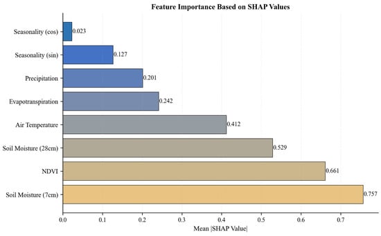
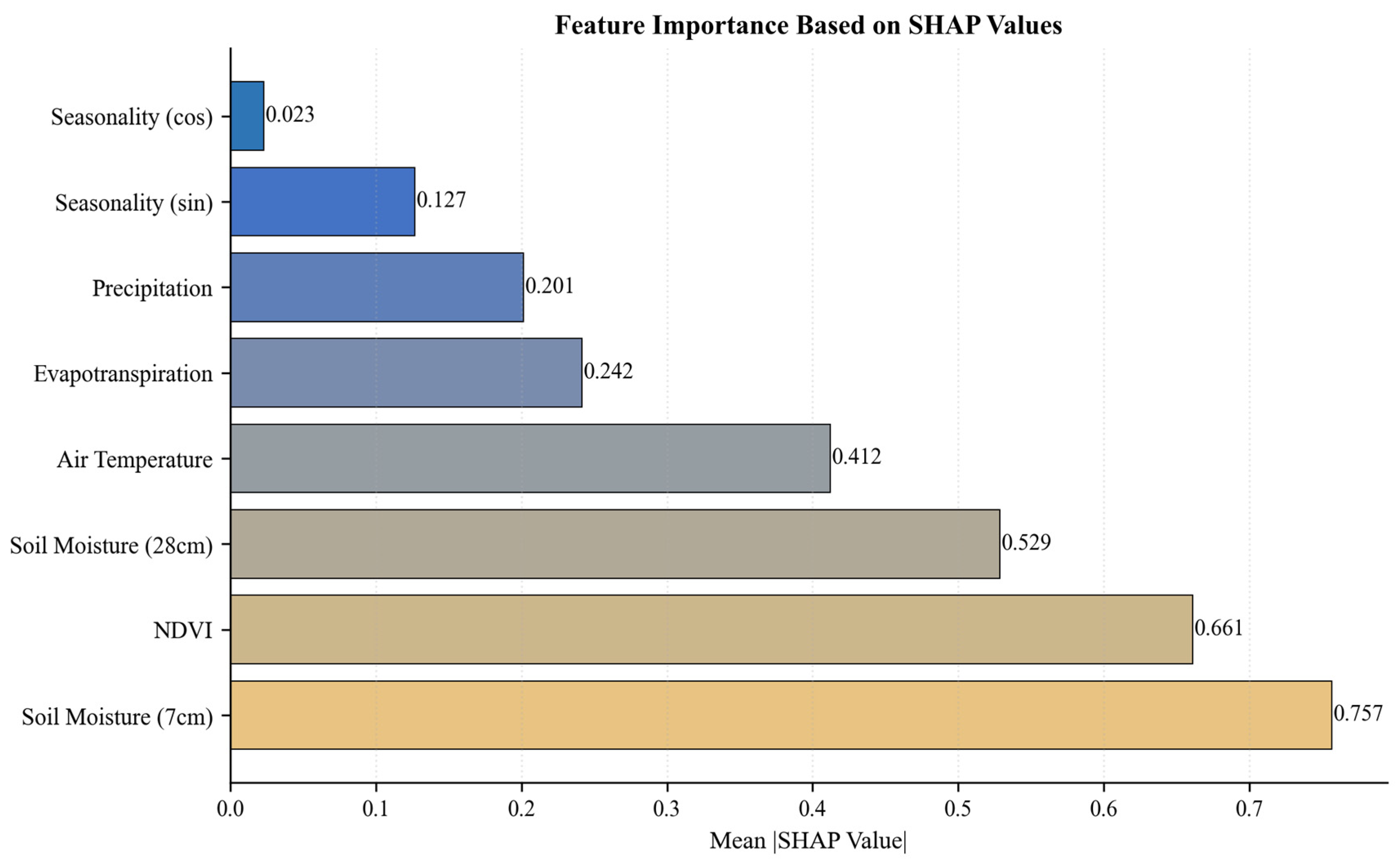
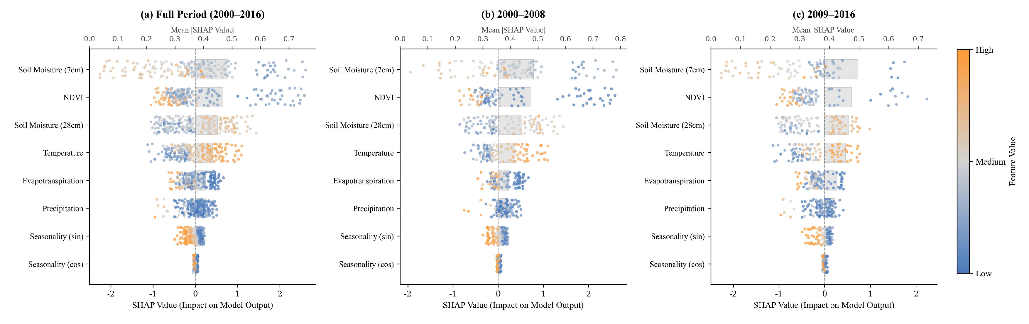
SHAP analysis across the entire period (2000–2016) indicates that surface soil moisture (7 cm) contributed the most (25.6%), highlighting the dominant role of surface hydrological processes in groundwater dynamics. NDVI contributed 22.4%. Combined with the regional ecological restoration context, this indicates significant vegetation-driven hydrological processes. This aligns with Wang et al. (2024)’s findings that groundwater depth in the West Liao River Basin is closely linked to vegetation development [51]. Deep soil moisture (28 cm), air temperature, evapotranspiration, and precipitation contributed 17.9%, 14.0%, 8.2%, and 6.8%, respectively, collectively forming a multifaceted combination of factors influencing the groundwater system. Feature importance analysis based on average absolute SHAP values (Figure 6) indicates that soil moisture (7 cm) makes the most significant contribution to groundwater level changes. Its importance is 1.13 times that of the second-ranked NDVI and 1.5 times the combined contribution of climatic factors (air temperature, precipitation, evapotranspiration). This quantitative ranking reveals the dominant role of soil moisture conditions in the evolution of groundwater in the West Liao River Basin. This aligns with the perspective proposed by Wang et al. [51], who suggested that a surge in groundwater supply has led to an imbalance between recharge and discharge.

Figure 6. Feature Importance Ranking Based on SHAP Values (Average Absolute SHAP Value).

A segmented comparison reveals that, with the 2009 inflection point as the boundary, the significance of temperature increased markedly in the later period (rate of change +22.3%), suggesting intensifying climate change pressures on the groundwater system. NDVI influence showed a weakening trend (−18.7%), while surface soil moisture influence slightly decreased (−7.0%), potentially reflecting adjustments from human activities, potentially reflecting changes in human activities or land management practices (such as shifts in agricultural practices, crop types, or water conservation measures). Seasonal components and evapotranspiration influence slightly strengthened, indicating heightened system sensitivity to climatic seasonality.

SHAP visualization results (Figure 7) further reveal the nonlinear characteristics of driving factors. The three-panel comparison shows that surface soil moisture and NDVI maintained high importance throughout the entire period, while temperature influence significantly increased in the later period. The SHAP value distribution for temperature exhibits pronounced negative skewness, consistent with the pressure of warming on groundwater resources. The high contribution of soil moisture underscores the importance of surface processes in groundwater dynamics.

Figure 7. Distribution of SHAP values for key drivers. (a) Full-period SHAP analysis; (b) Early-period (2000–2008) SHAP analysis; (c) Late-period (2009–2016) SHAP analysis.

In summary, soil moisture collectively contributed 43.5%, and climatic factors collectively contributed 29.0%, forming the primary driving system for groundwater level changes in the West Liao River Basin. This result aligns with spatiotemporal evolution patterns: the initial slower decline (−0.481 m/yr) corresponded to a pattern dominated by NDVI and soil moisture, a pattern consistent with the known regional trends of vegetation restoration and agricultural expansion during that period; while the accelerated decline in the later period (−0.749 m/yr) aligns with the intensifying influence of temperature. The dominant contribution of soil moisture to changes in groundwater depth highlights the critical role of surface hydrological processes in regional groundwater dynamics. It provides quantitative evidence for understanding the “nature-human” composite driving mechanism.

SHAP analysis indicates that soil moisture content is the most significant predictor of groundwater level variability in the West Liao River Basin; when surface and subsurface data are combined, the model achieves an explanatory power of 43.5%. In hydrological modeling, soil moisture dynamics are regulated not only by natural processes (precipitation, evapotranspiration) but also by human activities—particularly agricultural irrigation, which significantly alters soil moisture conditions during the growing season by artificially replenishing water. This finding is highly consistent with the regional context: previous studies have confirmed that irrigation accounts for 75–88.9% of total water use and is the primary driver of groundwater depletion [8]. Therefore, the significance of soil moisture content aligns closely with the region’s history of intensive agricultural irrigation, a pattern consistent with substantial anthropogenic influence in this region.

However, limitations should be noted: GLDAS soil moisture data primarily reflect surface–atmosphere interactions and do not directly measure groundwater extraction. Thus, while soil moisture is the dominant predictor, it cannot be directly interpreted as a quantitative proxy for irrigation intensity. Rather, it strongly indicates that hydrological processes—shaped by both natural and anthropogenic factors and centered on changes in soil moisture—play a primary regulatory role in regional groundwater dynamics.

3.3. Comparison of Model Prediction Performance

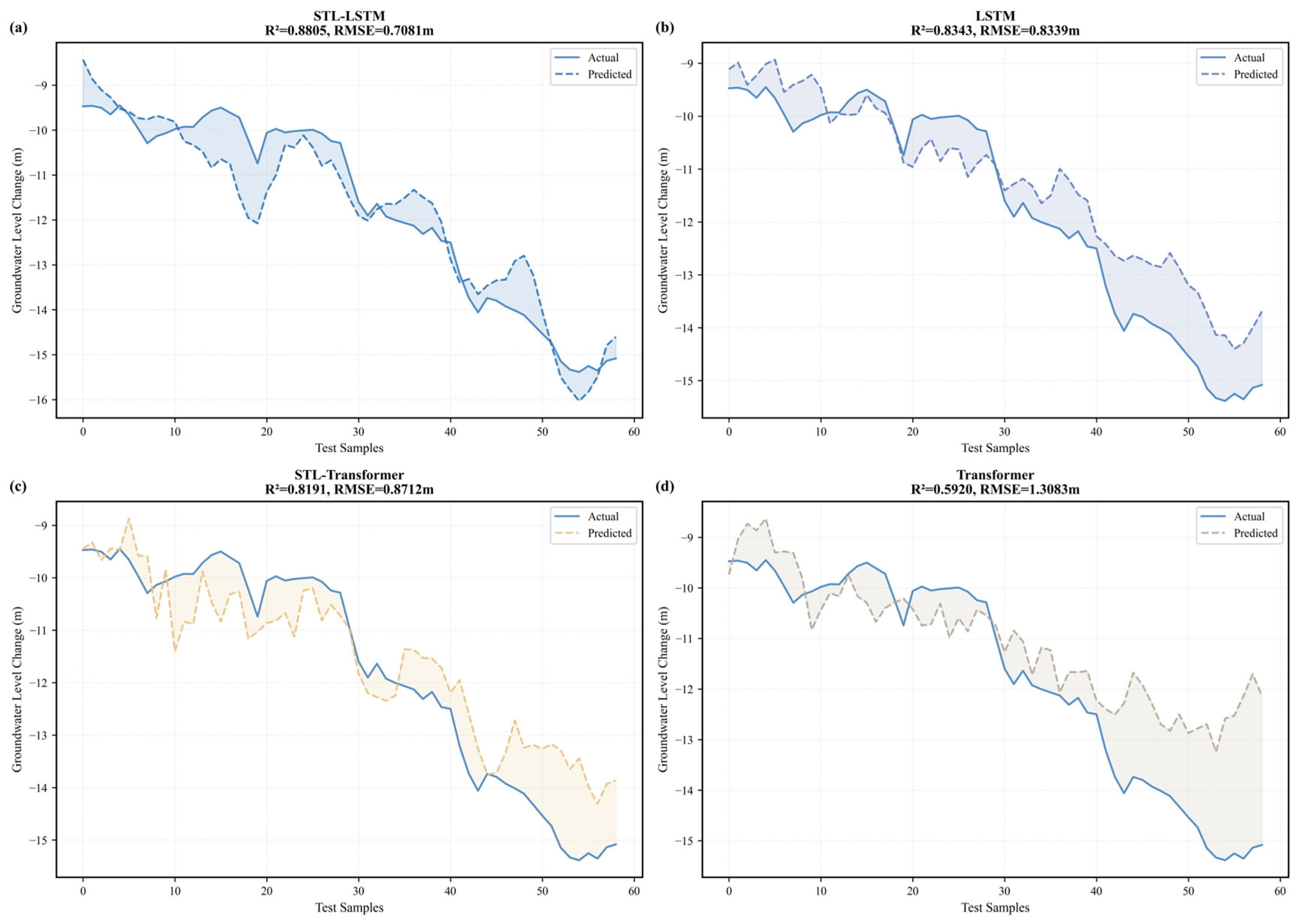
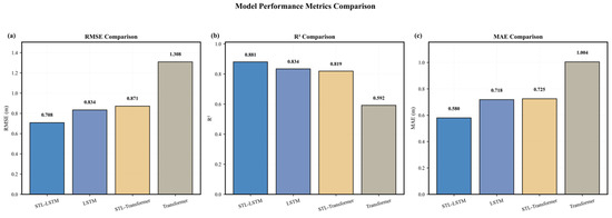
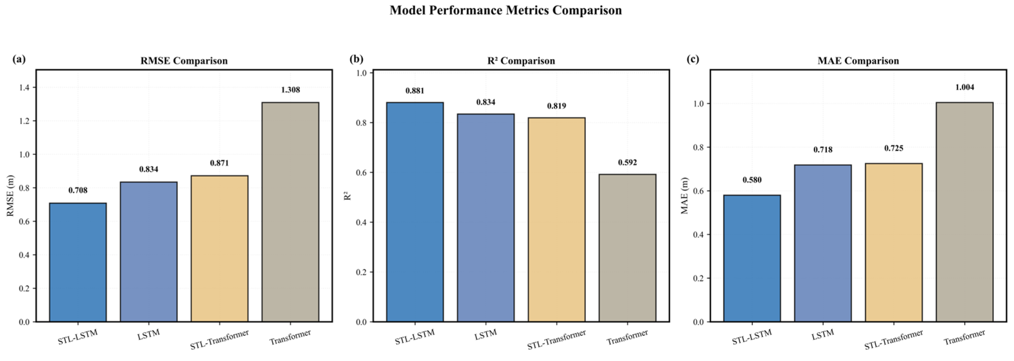
The four prediction models exhibit significant differences in performance on the test set. Quantitative evaluation results (Table 7) indicate that the STL-LSTM model achieved the best performance across all metrics, with a coefficient of determination of 0.8805, a root mean square error of 0.7081 m, and a mean absolute percentage error of 5.19%. This demonstrates the model’s high accuracy in predicting groundwater level changes in the West Liao River Basin. The LSTM model ranked second, with a coefficient of determination of 0.8343 and an RMSE of 0.8339 metres, demonstrating significantly better performance than the two Transformer-based models.

Table 7. Comparison of Model Prediction Performance (Sorted in Descending Order by R²).

Model	RMSE (m)	MAE (m)	R2	MAPE (%)
STL-LSTM	0.708	0.580	0.881	5.19
LSTM	0.834	0.718	0.834	5.85
STL-Transformer	0.871	0.725	0.819	6.01
Transformer	1.308	1.004	0.592	7.89

STL decomposition significantly enhances predictive performance. Compared to the baseline LSTM, STL-LSTM improves the coefficient of determination by 5.5% and reduces the root mean square error by 15.1% over LSTM. STL-Transformer achieves a remarkable 38.4% increase in the coefficient of determination and a 33.4% reduction in root mean square error compared to Transformer. The strong trendiness and seasonal characteristics of groundwater sequences in the West Liao River Basin enable STL decomposition to effectively separate components across different scales, helping models better learn the evolution patterns across various dimensions [44].

Comparing the prediction results over time (Figure 8), the STL-LSTM model exhibits the highest alignment with actual water level changes, particularly accurately capturing the inflection point during the accelerated decline phase in mid-2015. While the LSTM model generally follows the correct trend, it shows slightly larger deviations at certain inflection points. Accurate prediction of this inflection point has significant implications for regional groundwater overexploitation management, providing timely early warning support for “water-based management” control strategies [34]. The two Transformer-based models exhibited relatively larger prediction fluctuations and insufficient capture of long-term sequence trends. This may be attributed to the relatively short sequence length in this study, which failed to fully leverage the Transformer’s advantage in capturing long-term dependencies.

Figure 8. Sequential Comparison of Prediction Results Across Model. (a) STL-LSTM; (b) LSTM; (c) STL-Transformer; (d) Transformer. The shaded area indicates the prediction error between observations and predictions.

The bar chart (Figure 9) visually compares core metrics—RMSE, R², and MAE—across models. STL-LSTM demonstrated the best performance across all three metrics, with its R² value (0.8805) significantly higher than that of other models.

Figure 9. Comprehensive Comparison of Prediction Performance Metrics. (a) RMSE; (b) R²; (c) MAE.

The poor performance of the Transformer model can be attributed primarily to two factors: firstly, the dataset was too small (137 training samples), falling far short of the tens of thousands of samples required for its self-attention mechanism to function effectively; secondly, the historical window was too short (five months), limiting the model’s ability to capture long-range dependencies, which is precisely the core strength of the Transformer. This is consistent with existing research, which indicates that Transformers require larger datasets and longer sequences to outperform recurrent neural networks. It is worth noting that STL decomposition significantly improved model performance (R² increased by 38.4%), suggesting that pre-processing techniques can partially mitigate data constraints. The use of larger datasets and longer sequences in future studies is expected further to unlock the potential of Transformers in groundwater level prediction.

To validate the rationality of the selected historical window length, a sensitivity analysis of the window length was conducted (Figure 10). The results indicate that as the window length increases from 3 months to 12 months, the performance of the LSTM model first improves and then declines; the 9-month window achieves the optimal performance (RMSE = 0.7046 m), while the 5-month window (RMSE = 0.8339 m) differs from the optimal window by only 15.5%. Taking into account data utilization (the 9-month window reduces the number of training samples by 4), real-time requirements, and computational efficiency, the 5-month window balances practical application needs while ensuring high accuracy. Therefore, selecting a 5-month window as the final historical window length is reasonable and effective.

Figure 10. Model Performance (RMSE) under Different Window Lengths.

3.4. Discussion

Soil moisture, as the dominant factor (43.5%) in groundwater variability, highlights the crucial role of surface hydrological processes, indicating that groundwater dynamics in the West Liao River Basin are primarily controlled by anthropogenically modulated surface processes rather than purely climatic variability.

The STL-LSTM model (R² = 0.8805) demonstrates the effectiveness of combining time-series decomposition with deep learning for processing non-stationary hydrological data. The poor performance of the Transformer model suggests that such architectures require larger datasets, which is of reference value for hydrological studies with limited data.

This study has limitations, including a lack of direct irrigation data and the ‘black-box’ nature of the models. Future work should integrate remote-sensing irrigation data to quantify anthropogenic disturbances and explore the use of physically constrained neural networks to enhance interpretability. From a management perspective, this predictive framework can provide early warnings of groundwater depletion for the ‘water-based demand’ approach in the West Liao River Basin, assisting decision-makers in optimising crop patterns and irrigation schedules to prevent ecological degradation caused by falling water levels [52]. It also provides a basis for assessing water resource carrying capacity, thereby contributing to improved agricultural water use efficiency and the sustainable utilisation of groundwater, and safeguarding the ecological and food security of the ‘Golden Corn Belt’ [53].

4. Conclusions

This study investigates the West Liao River Basin using groundwater level monitoring data from 2000 to 2016. By integrating STL time series decomposition, abrupt change detection, random forest-SHAP attribution analysis, and deep learning prediction models, this study systematically analyses the spatiotemporal evolution patterns and key driving mechanisms of groundwater levels, establishing a high-precision prediction model. Key findings are as follows:

(1)

Groundwater levels exhibit a sustained decline trend, with 2009 identified as a critical inflection point. The basin experienced a cumulative decline of 15.27 m, with a spatial pattern of “higher in the west, lower in the east,” and the most significant decrease occurring in the Hongshan area. Breakpoint analysis revealed that the decline rate accelerated significantly from −0.481 m/yr before 2009 to −0.749 m/yr after 2009, representing a 55.7% increase.

(2)

Statistical attribution indicates that soil moisture (43.5%) and climatic factors (29.0%) are the primary predictors of groundwater variability. SHAP analysis reveals that surface soil moisture (7 cm) contributes the most (25.6%), followed by deep soil moisture (17.9%); together, these account for 43.5% of the total variation. The dominant role of soil moisture highlights the critical importance of agricultural irrigation; in this intensively irrigated region, agricultural irrigation has significantly altered soil water dynamics. Climate factors (including air temperature, evapotranspiration and precipitation) contributed a total of 29.0%. Notably, the influence of air temperature increased significantly during the later stages of the transition, confirming the continuing intensification of pressures resulting from climate change.

(3)

The STL-LSTM hybrid model demonstrated optimal predictive performance in this study area. Compared to LSTM, Transformer, and STL-Transformer models, STL-LSTM achieved the highest coefficient of determination (0.8805), lowest root mean square error (0.7081 m), and an average absolute percentage error of only 5.19%, significantly enhancing the prediction accuracy and robustness for non-stationary groundwater series.

This study provides a scientific basis for regional groundwater management in the West Liao River Basin through an integrated framework combining trend diagnosis, driver attribution, and hybrid forecasting. Future work should integrate higher spatiotemporal resolution irrigation data to develop more physically interpretable models, thereby enhancing the decision-support capacity of predictions.

References

- Saito, L.; Christian, B.; Diffley, J.; Richter, H.; Rohde, M.M.; Morrison, S.A. Managing groundwater to ensure ecosystem function. Groundwater 2021, 59, 322–333. [Google Scholar] [CrossRef] [Scilit] [PubMed]
- Gleeson, T.; Cuthbert, M.; Ferguson, G.; Perrone, D. Global groundwater sustainability, resources, and systems in the Anthropocene. Annu. Rev. Earth Planet. Sci. 2020, 48, 431–463. [Google Scholar] [CrossRef] [Scilit]
- Perez, N.; Singh, V.; Ringler, C.; Xie, H.; Zhu, T.; Sutanudjaja, E.H.; Villholth, K.G. Ending groundwater overdraft without affecting food security. Nat. Sustain. 2024, 7, 1007–1017. [Google Scholar] [CrossRef] [Scilit]
- Karandish, F.; Liu, S.; de Graaf, I. Global groundwater sustainability: A critical review of strategies and future pathways. J. Hydrol. 2025, 657, 133060. [Google Scholar] [CrossRef] [Scilit]
- Li, X.; Xu, X.; Tian, W.; Tian, J.; He, C. Contribution of climate change and vegetation restoration to interannual variability of evapotranspiration in the agro-pastoral ecotone in northern China. Ecol. Indic. 2023, 154, 110485. [Google Scholar] [CrossRef] [Scilit]
- Zhong, Y.; Zhong, M.; Feng, W.; Zhang, Z.; Shen, Y.; Wu, D. Groundwater depletion in the West Liaohe River Basin, China and its implications revealed by GRACE and in situ measurements. Remote Sens. 2018, 10, 493. [Google Scholar] [CrossRef] [Scilit]
- Xu, Y.; Yang, D.; Tang, L.; Qiao, Z.; Ma, L.; Chen, M. Evaluating main drivers of terrestrial water storage depletion in the agro-pastoral ecotone of northern China. J. Hydrol. 2023, 626, 130242. [Google Scholar] [CrossRef] [Scilit]
- Gao, Z.; He, J.; Dong, K.; Li, X. Trends in reference evapotranspiration and their causative factors in the West Liao River basin, China. Agric. For. Meteorol. 2017, 232, 106–117. [Google Scholar] [CrossRef] [Scilit]
- Yu, Y.; Zhang, G.; Qi, P.; Sun, J.; Zhang, Q.; Hu, B.; Xu, Y. Irrigated agriculture expansion drives groundwater storage decline in Black Soil Region of Northeast China. Agric. Water Manag. 2025, 319, 109813. [Google Scholar] [CrossRef] [Scilit]
- Gao, M.; Liu, Q.; Liu, Y.; Yang, N.; Wang, Y.; Li, X. Spatial and temporal variations of vegetation water use efficiency and its response to climate change and human activities in the West Liao River Plain, China. Front. Ecol. Evol. 2023, 11, 1176131. [Google Scholar] [CrossRef] [Scilit]
- Kuang, X.; Liu, J.; Scanlon, B.R.; Jiao, J.J.; Jasechko, S.; Lancia, M.; Biskaborn, B.K.; Wada, Y.; Li, H.; Zeng, Z.; et al. The changing nature of groundwater in the global water cycle. Science 2024, 383, eadf0630. [Google Scholar] [CrossRef] [Scilit]
- Adams, K.H.; Reager, J.T.; Rosen, P.; Wiese, D.N.; Farr, T.G.; Rao, S.; Haines, B.J.; Argus, D.F.; Liu, Z.; Smith, R.; et al. Remote sensing of groundwater: Current capabilities and future directions. Water Resour. Res. 2022, 58, e2022WR032219. [Google Scholar] [CrossRef] [Scilit]
- Jasechko, S.; Seybold, H.; Perrone, D.; Fan, Y.; Shamsudduha, M.; Taylor, R.G.; Fallatah, O.; Kirchner, J.W. Rapid groundwater decline and some cases of recovery in aquifers globally. Nature 2024, 625, 715–721. [Google Scholar] [CrossRef] [Scilit]
- Zhao, Z.; Lin, A.; Feng, J.; Yang, Q.; Zou, L. Analysis of water resources in Horqin Sandy Land using multisource data from 2003 to 2010. Sustainability 2016, 8, 374. [Google Scholar] [CrossRef] [Scilit]
- Liu, K.; Zhang, J.; Wang, M. Drivers of groundwater change in China and future projections. Remote Sens. 2022, 14, 4825. [Google Scholar] [CrossRef] [Scilit]
- Green, T.R.; Taniguchi, M.; Kooi, H.; Gurdak, J.J.; Allen, D.M.; Hiscock, K.M.; Treidel, H.; Aureli, A. Beneath the surface of global change: Impacts of climate change on groundwater. J. Hydrol. 2011, 405, 532–560. [Google Scholar] [CrossRef] [Scilit]
- Jesse, G.; Boateng, C.D.; Aryee, J.N.; Osei, M.A.; Wemegah, D.D.; Gidigasu, S.S.; Britwum, A.; Afful, S.K.; Touré, H.; Mensah, V.; et al. A systematic review of machine learning models for groundwater level prediction. Appl. Comput. Geosci. 2025, 28, 100303. [Google Scholar] [CrossRef] [Scilit]
- Dhapre, M.; Jadhav, S.; Das, D.; Khan, J.; Kim, Y.; Chiao, S.; Danielson, T. A systematic review of machine learning in groundwater monitoring. Environ. Model. Softw. 2025, 192, 106549. [Google Scholar] [CrossRef] [Scilit]
- Zhang, Q.; Li, P.; Ren, X.; Ning, J.; Li, J.; Liu, C.; Wang, Y.; Wang, G. A new real-time groundwater level forecasting strategy: Coupling hybrid data-driven models with remote sensing data. J. Hydrol. 2023, 625, 129962. [Google Scholar] [CrossRef] [Scilit]
- Obergfell, C.; Bakker, M.; Maas, K. Identification and explanation of a change in the groundwater regime using time series analysis. Groundwater 2019, 57, 881–893. [Google Scholar] [CrossRef] [Scilit] [PubMed]
- Talib, A.; Desai, A.R.; Huang, J. Spatial and temporal forecasting of groundwater anomalies in complex aquifer undergoing climate and land use change. J. Hydrol. 2024, 639, 131525. [Google Scholar] [CrossRef] [Scilit]
- Boo, K.B.W.; El-Shafie, A.; Othman, F.; Khan, M.M.H.; Birima, A.H.; Ahmed, A.N. Groundwater level forecasting with machine learning models: A review. Water Res. 2024, 267, 121249. [Google Scholar] [CrossRef] [Scilit]
- Zhu, F.; Han, M.; Sun, Y.; Zeng, Y.; Zhao, L.; Zhu, O.; Hou, T.; Zhong, P.-A. A machine learning framework for multi-step-ahead prediction of groundwater levels in agricultural regions with high reliance on groundwater irrigation. Environ. Model. Softw. 2024, 180, 106146. [Google Scholar] [CrossRef] [Scilit]
- Lafare, A.E.A.; Peach, D.W.; Hughes, A.G. Use of seasonal trend decomposition to understand groundwater behaviour in the Permo-Triassic Sandstone aquifer, Eden Valley, UK. Hydrogeol. J. 2016, 24, 141–158. [Google Scholar] [CrossRef] [Scilit]
- Liu, W.; Yu, H.; Yang, L.; Yin, Z.; Zhu, M.; Wen, X. Deep learning-based predictive framework for groundwater level forecast in arid irrigated areas. Water 2021, 13, 2558. [Google Scholar] [CrossRef] [Scilit]
- Attea, Z.H.; Hassan, W.H.; Al-Shammari, M.H. Integration of MODFLOW and deep learning models for groundwater level prediction. Results Eng. 2025, 27, 106268. [Google Scholar] [CrossRef] [Scilit]
- Sun, K.; Hu, L.; Sun, J.; Cao, X. Enhancing groundwater level prediction accuracy at a daily scale through combined machine learning and physics-based modeling. J. Hydrol. Reg. Stud. 2023, 50, 101577. [Google Scholar] [CrossRef] [Scilit]
- Nazari, A.; Jamshidi, M.; Roozbahani, A.; Golparvar, B. Groundwater level forecasting using empirical mode decomposition and wavelet-based long short-term memory (LSTM) neural networks. Groundw. Sustain. Dev. 2025, 28, 101397. [Google Scholar] [CrossRef] [Scilit]
- Cui, X.; Wang, Z.; Xu, N.; Wu, J.; Yao, Z. A secondary modal decomposition ensemble deep learning model for groundwater level prediction using multi-data. Environ. Model. Softw. 2024, 175, 105969. [Google Scholar] [CrossRef] [Scilit]
- Cai, H.; Liu, S.; Shi, H.; Zhou, Z.; Jiang, S.; Babovic, V. Toward improved lumped groundwater level predictions at catchment scale: Mutual integration of water balance mechanism and deep learning method. J. Hydrol. 2022, 613, 128495. [Google Scholar] [CrossRef] [Scilit]
- Sun, J.; Hu, L.; Li, D.; Sun, K.; Yang, Z. Data-driven models for accurate groundwater level prediction and their practical significance in groundwater management. J. Hydrol. 2022, 608, 127630. [Google Scholar] [CrossRef] [Scilit]
- Huang, X.; Li, Y.N. Analysis of water resources variation trend in the Xiliaohe River Basin of Inner Mongolia. In Proceedings of the 2021 Academic Annual Conference of the Chinese Hydraulic Engineering Society; China Water & Power Press: Beijing, China, 2021; pp. 293–297. [Google Scholar]
- Wang, Z.; Zhao, H.; Zhao, C. Temporal and spatial evolution characteristics of land use and landscape pattern in key wetland areas of the West Liao River Basin, Northeast China. J. Environ. Eng. Landsc. Manag. 2022, 30, 195–205. [Google Scholar] [CrossRef] [Scilit]
- Yang, Y.; Liu, D.X. Understanding and thoughts on the “Water-Based Development” work in the Xiliaohe River Basin of Inner Mongolia. Water Resour. Dev. Res. 2022, 22, 94–97. (In Chinese) [Google Scholar]
- Wang, Y.D.; Ma, S.Q.; Li, L.; Guo, F. Some thoughts on “Water-Based Development” in the Xiliaohe River Basin of Inner Mongolia. Inn. Mong. Water Resour. 2023, 44, 6–9. (In Chinese) [Google Scholar]
- Moran, P.A.P. Notes on continuous stochastic phenomena. Biometrika 1950, 37, 17–23. [Google Scholar] [CrossRef] [Scilit] [PubMed]
- Cleveland, R.B.; Cleveland, W.S.; McRae, J.E.; Terpenning, I. STL: A seasonal-trend decomposition procedure based on loess. J. Off. Stat. 1990, 6, 3–73. [Google Scholar]
- Mann, H.B. Nonparametric tests against trend. Econometrica 1945, 13, 245–259. [Google Scholar] [CrossRef] [Scilit]
- Breiman, L. Random Forests. Mach. Learn. 2001, 45, 5–32. [Google Scholar] [CrossRef] [Scilit]
- Lundberg, S.M.; Lee, S.I. A unified approach to interpreting model predictions. In Proceedings of the 31st Annual Conference on Neural Information Processing Systems (NeurIPS), Long Beach, CA, USA, 4–9 December 2017. [Google Scholar]
- Greff, K.; Srivastava, R.K.; Koutník, J.; Steunebrink, B.R.; Schmidhuber, J. LSTM: A search space odyssey. IEEE Trans. Neural Netw. Learn. Syst. 2017, 28, 2222–2232. [Google Scholar] [CrossRef] [Scilit]
- Vaswani, A.; Shazeer, N.; Parmar, N.; Uszkoreit, J.; Jones, L.; Gomez, A.N.; Kaiser, Ł.; Polosukhin, I. Attention is all you need. In Proceedings of the 31st Annual Conference on Neural Information Processing Systems (NeurIPS), Long Beach, CA, USA, 4–9 December 2017. [Google Scholar]
- Kumar, R.; Kumar, P.; Kumar, Y. Integrating big data driven sentiments polarity and ABC-optimized LSTM for time series forecasting. Multimed. Tools Appl. 2022, 81, 34595–34614. [Google Scholar] [CrossRef] [Scilit]
- Yan, L.J.; He, X.; Lu, C.Y.; Liu, J.X.; Ma, F.H.; Li, Z.P. Variation trend and over-exploitation analysis of groundwater depth in the Xiliaohe Plain. Hydrology 2021, 41, 96–102. (In Chinese) [Google Scholar]
- Chai, Z.F.; Bai, M.Z.; Kuai, T.; Wang, X.C. Study on agricultural irrigation area and irrigation water consumption in the Xiliaohe River Basin of Inner Mongolia based on multi-temporal remote sensing images. Inn. Mong. Water Resour. 2023, 12, 6–7. (In Chinese) [Google Scholar]
- Yu, Y.X.; Zhang, G.X.; Sun, J.X.; Wu, Y.F.; Zhang, Q.S.; Li, B. Variation characteristics and driving factors of groundwater storage in the Xiliaohe River Basin. South-to-North Water Transf. Water Sci. Technol. 2025, 23, 975–986. (In Chinese) [Google Scholar]
- Haacker, E.M.K.; Kendall, A.D.; Hyndman, D.W. Water level declines in the High Plains Aquifer: Predevelopment to resource senescence. Groundwater 2016, 54, 231–242. [Google Scholar] [CrossRef] [Scilit]
- Scanlon, B.R.; Faunt, C.C.; Longuevergne, L.; Reedy, R.C.; Alley, W.M.; McGuire, V.L.; McMahon, P.B. Groundwater depletion and sustainability of irrigation in the US High Plains and Central Valley. Proc. Natl. Acad. Sci. USA 2012, 109, 9320–9325. [Google Scholar] [CrossRef] [Scilit] [PubMed]
- Walker, G. A potential approach of reporting risk to baseflow from increased groundwater extraction in the Murray-Darling Basin, South-Eastern Australia. Water 2022, 14, 2118. [Google Scholar] [CrossRef] [Scilit]
- Feng, W.; Shum, C.K.; Zhong, M.; Pan, Y. Groundwater storage changes in China from satellite gravity: An overview. Remote Sens. 2018, 10, 674. [Google Scholar] [CrossRef] [Scilit]
- Wang, X.; Guo, L.; Hu, C.; Zhou, L.; Sun, J.Y.; Zhao, J. Exploration of the relationship between groundwater and vegetation development in the Xiliaohe River Basin based on RS and GIS. Ground Water 2024, 46, 20–22+70. (In Chinese) [Google Scholar]
- Tang, S.N.; Ding, Y.Y.; Yu, L.L.; Zhang, Y.; Chen, F.; Guan, X.; Ma, S.Q.; Wang, Q. The idea of “the demand and management for water resources are determined by water quantity” in Xiliao River Basin, Inner Mongolia. Water Resour. Plan. Des. 2019, 36, 28–31. (In Chinese) [Google Scholar]
- Fu, Y.H. Groundwater resources development and ecological environmental protection strategies in Chifeng City. China Resour. Compr. Util. 2025, 43, 163–165+169. (In Chinese) [Google Scholar]
Disclaimer/Publisher’s Note: The statements, opinions and data contained in all publications are solely those of the individual author(s) and contributor(s) and not of MDPI and/or the editor(s). MDPI and/or the editor(s) disclaim responsibility for any injury to people or property resulting from any ideas, methods, instructions or products referred to in the content. |
© 2026 by the authors. Licensee MDPI, Basel, Switzerland. This article is an open access article distributed under the terms and conditions of the Creative Commons Attribution (CC BY) license.