An Efficient Real-Time Anomaly Detection Scheme for Water Quality Monitoring ^†

Abstract

Maintaining high quality of water resources is essential to the physical health of mankind and sustainable development of society. Accordingly, it is necessary to detect anomalies in water quality variations, which may be caused by pollution. However, prompt anomaly detection is a challenging task, either demanding a lot of human effort or yielding low accuracy, due to the nonlinear and non-stationary characteristics of water quality data. In this paper, we present an efficient real-time anomaly detection scheme which boosts detection accuracy while mitigating human effort. The scheme takes a prediction–detection–verification approach in which a deep learning prediction model is built from historical data and is used to predict future values. The predicted values are compared with the actual measurements, and the residuals are inspected by a detection model. An alarm is sent to field engineers for verification for each anomaly detected by the detection model, and the verification result is analyzed by the scheme to maintain high prediction and detection accuracy. Experiments on multiple water quality datasets show that the proposed scheme achieves significantly higher recall rates and lower false alarm rates in almost all test scenarios, compared with schemes that do not utilize verification.

1. Introduction

Clean water resources are vital to mankind’s survival and development. However, with population growth and economic development around the world, many surface water resources are contaminated by various pollutants, putting human health at risk [1,2]. Prompt detection of water pollution becomes critical to surface water resource protection. In order to continually monitor the quality of surface water resources, governments and organizations have deployed monitoring stations in many water bodies that regularly measure water quality parameters. When water is polluted, values of some water quality parameters usually deviate from normal values, i.e., they stand out as anomalies among the data. Thus by detecting anomalies in water quality measurements, we may discover whether a pollution event has occurred to the water body.

Traditionally, researchers used mechanistic models, such as the Streeter–Phelps model, for water quality modeling and anomaly detection [3,4]. A mechanistic model requires extensive hydrological and meteorological knowledge as well as information of the specific water body, and thus is very difficult to establish. Moreover, even if such a model fits well for a certain water body, it may be hard to adapt to other water bodies.

Therefore, more researchers have turned to the data-driven approach, which relies on the historical data collected through a long period instead of complex expertise in hydrology. Data-driven statistical methods, such as autoregression and principal component analysis, have been frequently used in anomaly detection for water quality as well as other time series data [5,6].

Recently, with the fast development of artificial intelligence, machine learning techniques (including deep learning) have been widely adopted in anomaly detection. Such methods are also data-driven, but they are more capable of catching the intrinsic nonlinear and non-stationary characteristics of water quality data than pure statistical methods, and thus are more effective in anomaly detection.

One group of machine learning-based anomaly detection schemes conquers the issue directly based on the water quality measurements. Bi [7] and Liu [8] adopted a supervised learning approach and built classification models, using Convolutional Neural Network (CNN) or Long Short-Term Memory (LSTM), to detect anomalies in the time series of water quality measurements. Supervised learning approaches require data labeling and thus involve extra labor costs. On the other hand, Bourelly [9] and others [10,11,12] adopted an unsupervised learning approach using algorithms such as Local Outlier Factor, Isolation Forest, or Hidden Markov Model, while Audibert [13] used an adversarial training framework, consisting of two autoencoders, to detect anomalies in time sequences also in an unsupervised way. To deal with the nonlinear and non-stationary characteristics of the water quality data, Jiang [14], Ni [15], and Zhang [16] extracted relatively stable features from the measurements as the first step, using techniques such as Fourier transform and wavelet transform, then applied supervised or unsupervised learning algorithms to find outliers in the features which denote the anomalies in the original measurements.

Anomalies are behaviors that deviate from normal patterns. Given a sufficiently long sequence of normal water quality measurements, through statistical or machine learning methods, prediction models may be established that essentially describe the normal fluctuation patterns of the data and can be used to predict future values in the sequence [17,18,19]. Thus the second group of machine learning-based anomaly detection schemes builds prediction models and utilizes the differences between actual measurements and predicted values (known as prediction residuals) to detect anomalies, where a larger prediction residual often indicates a higher probability of anomaly. For example, Li et al. proposed an anomaly scoring scheme for general time sequences, in which an LSTM model was used to predict future values, and anomaly scores were computed according to the prediction residuals and compared with a dynamically adjusted threshold to determine anomalies [20]. For time series of water quality measurements, Liu et al. [21] used a Bayesian autoregressive model and Wang et al. [22] used an LSTM model for prediction; both of their works used Isolation Forest to detect anomalies in the prediction residuals. Liao et al. [23] and Jiang et al. [24] also proposed prediction-based frameworks for anomaly detection.

All these studies showed that anomaly detection based on prediction residuals achieves higher accuracy than using actual measurements directly. However, they did not explicitly specify a viable scheme for real-world application. When a pollution event occurs, the water quality measurements become anomalous, which may be detected by an anomaly detection scheme. Naturally, what the measurements would be if the pollution had not occurred is unknown. Yet a prediction-based scheme needs to maintain normal historical data in order to predict normal future values. Using anomalous data as part of input to the prediction model would apparently distort the output of the model. Therefore, a mechanism that maintains the normality of the historical data must be incorporated into a prediction-based anomaly detection scheme in order for the scheme to be viable for real-world application.

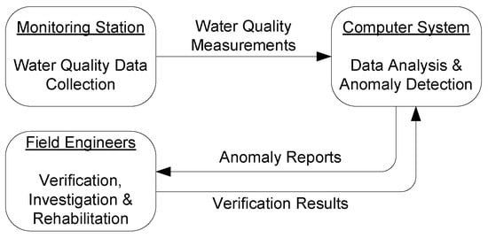
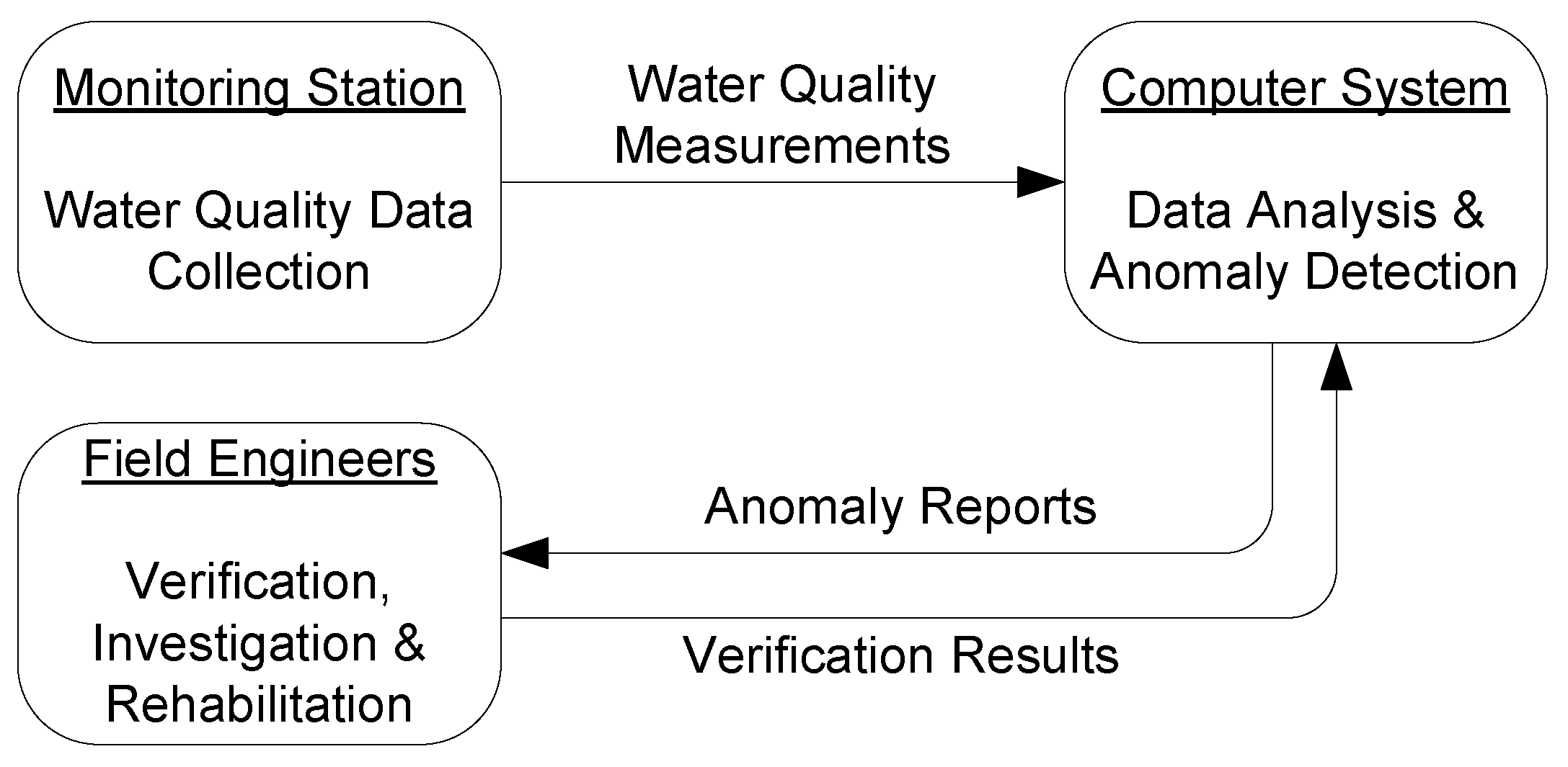
In real world, a typical water quality monitoring system often consists of one or more monitoring stations, a computer system, and a team of field engineers, as shown in Figure 1. The monitoring stations periodically collect water quality data and send them to the computer system. The computer system stores and analyzes the data. The use of the computer system greatly reduces human labor since there is no need for the field engineers to regularly check the health of the water body in normal situations. However, once the computer system detects an anomaly in the data, which indicates a possible occurrence of pollution, it promptly sends an alarm to the field engineers. The field engineers then verify if the anomaly detected is indeed the result of pollution, investigate its cause if so, and try to rehabilitate the water condition. The verification result, whether the alarm is a true positive (meaning water pollution actually happened) or a false one, if sent back to the computer system, can be used by the latter to enhance the detection accuracy for future events. While human verification is an indispensable component of a practical water quality monitoring system, most of the existing research does not utilize it in anomaly detection.

Figure 1. Framework of a typical water quality monitoring system.

In addition, due to various reasons, water quality data collected from the monitoring stations in the field may experience occasional missing values or errors [25,26]. Existing prediction-based schemes often presume a well-established long history of data, which may not be available in reality. A practical solution should be adaptive to imperfect histories.

On the other hand, some existing schemes analyze an entire time sequence to find anomalies in the sequence, implicitly using future information (in the later part of the sequence) for the detection of past events (in the earlier part of the sequence) [20]. Such approaches are not proper for real-time detection.

To address these issues, in this study, we propose a novel anomaly detection scheme for water quality monitoring, named PADSV (prediction-based anomaly detection with selective verification). PADSV takes a prediction–detection–verification approach. The scheme adopts a deep learning model to predict future water quality based on the historical data. When an actual measurement is reported by the monitoring station, the prediction residual, which is the difference between the predicted data and the measurement, is computed. The residual is passed to a detection model which computes an anomaly score for the residual. The anomaly score is compared with a threshold to determine whether the current measurement indicates an anomaly, and an alarm is sent to the field engineers if so. The verification result from the field engineers is used to maintain accurate prediction and detection for future values and events.

Using self-collected datasets with simulated anomalies and a public water quality dataset from real world, we evaluated PADSV along with some reference schemes. The results show that PADSV achieved significantly higher recall rates and lower false alarm rates in almost all test scenarios, compared with a state-of-the-art anomaly detection algorithm as well as similar schemes that do not utilize human verification.

The main contribution of our work is as follows.

• The detection process in the proposed scheme is truly real-time. Only the recorded normal data are used to determine whether the current measurement is an anomaly. And the result is promptly generated soon after the measurement arrives.
• The proposed scheme is efficient in that it greatly reduces human labor. While the scheme does rely on verification by the field engineers, only raised alarms need to be verified manually, which are only a small portion of detection results, since anomalies are rare events in reality [27,28]. Moreover, as shown in the experimental results, the performance of the scheme is hardly affected by occasional verification misses, which further alleviates the burden of the field engineers. In addition, unlike the classification-based schemes [7,8], this scheme does not require data labeling. This makes the scheme more viable for real-world use.
• The proposed scheme builds its prediction and detection models based on segmented sequences of normal data, instead of relying on a fully consecutive sequence of historical data. This is consistent with the reality that normal data sequences are interrupted by occasional anomalies as well as missing values.

This work is an extension of our prior work [29]. Based on the preliminary idea of PADSV presented in [29], this work gives a full description of the scheme and evaluates it with more extensive data and experiments. To the best of our knowledge, PADSV is the first work that takes human verification into consideration in water quality anomaly detection.

The rest of the paper is organized as follows. Section 2 elaborates on the proposed PADSV scheme, the datasets used in the study, and the evaluation methodology. Section 3 presents the experimental results. Section 4 discusses the findings of our study as well as the limitations of the scheme.

2. Methods and Materials

In this section, we present the PADSV scheme, which integrates deep learning-based prediction, Isolation Forest-based anomaly detection, and verification-based model updating. We also give a description of the datasets, the anomaly models, and the metrics that were used to evaluate the performance of the scheme.

2.1. The PADSV Scheme

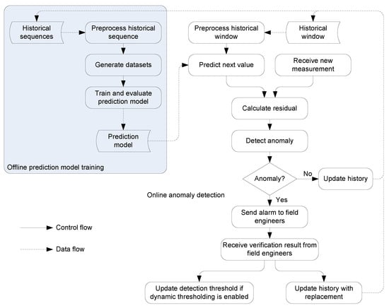
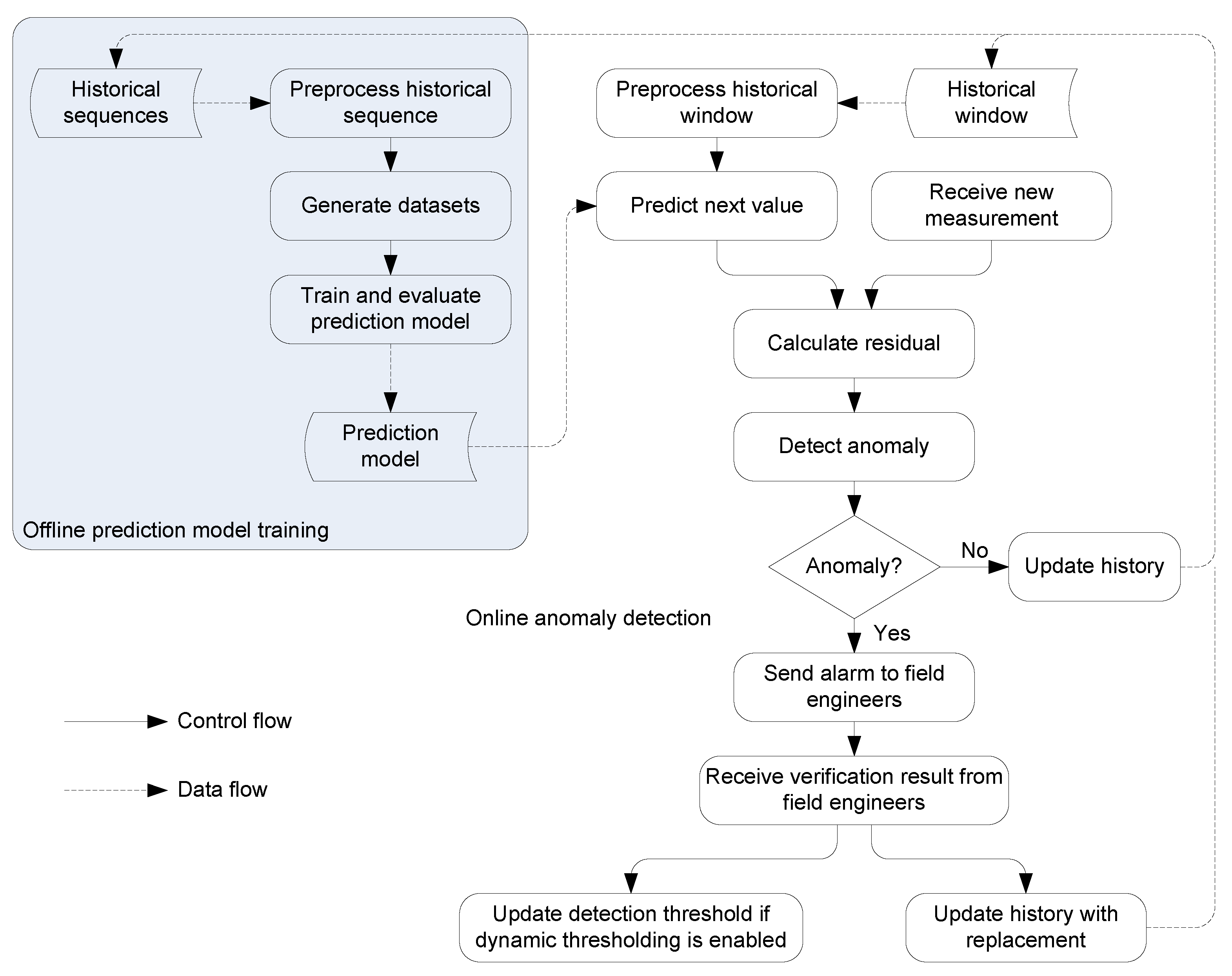
Figure 2 shows the flowchart of the PADSV scheme. The scheme consists of an offline prediction model training process and an online prediction-based anomaly detection process. The offline process, which runs at regular intervals, uses the long-term historical sequence of water quality measurements (possibly multiple sequences separated by anomalies and missing values) to train and evaluate the prediction model.

Figure 2. Flowchart of PADSV.

The online process, which runs in real time, predicts the next value based on the prediction model and a small window of recent data (i.e., historical window) once it receives a new measurement from the monitoring station. Then the residual between the predicted value and the measurement is calculated. Using an Isolation Forest-based anomaly detection model, the process computes an anomaly score for each residual.

Internally the online process maintains a threshold. If the anomaly score of a residual exceeds the threshold, which indicates that the current measurement significantly deviates from the normal variation pattern of the water quality, then the measurement is regarded as an anomaly. An alarm is sent to the field engineers, who verify whether it is a true anomaly (for example, some sort of pollution did occur) or a false alarm. The result of verification is sent back to the anomaly detection process. The historical sequence and historical window are updated according to the verification result. The threshold is also updated if dynamic thresholding is enabled. Since only the measurements that trigger alarms are verified by the field engineers, the verification is rather selective. By selective verification, the scheme greatly reduces human labor in water quality monitoring. More details of the scheme are elaborated in the following subsections.

In order for the scheme to work, we made the following assumptions.

1.

A sufficient amount of normal data have been collected to train the prediction model.

2.

When the scheme detects an anomaly and raises an alarm, field engineers put forth their best effort to verify it, and give the correct verification result if they finish verification before the next measurement time.

Assumption 1 ensures that the prediction model in our scheme can be initially trained to reflect the normal patterns of the water quality data. Note that the building of the models does not require the sequence of historical data to be continuous. In the real world, sporadic missing values do occur, breaking the time sequence into segments. Moreover, in our scheme, when the models are re-trained with newly accumulated data to reflect the current trend, confirmed anomalous measurements should not be used and should be excluded from the historical sequence, inevitably causing missing values in the sequence. In our study, more than four years of data from the same monitoring station in normal situations were used to train and validate the initial prediction model.

Assumption 2 was established because the detection performance of our scheme relies on the verification results from the field engineers. While having correct verification for each alarm is desirable, to achieve acceptable performance, only a portion of alarms need to be verified, as shown in our experiments, which makes the scheme more viable in reality. However, this assumption also implies that the field engineers do not give incorrect verification results.

2.1.1. Prediction

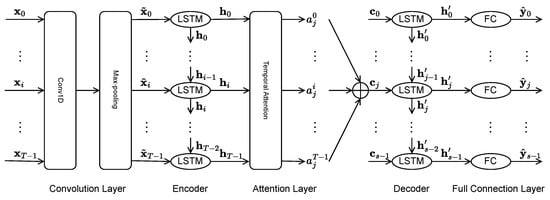
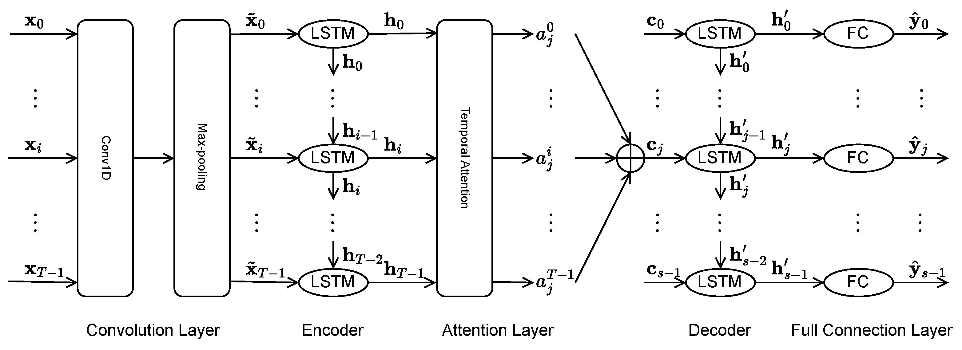
While there were many prediction models for time sequences, we adopted the deep learning model that we had proposed in our previous work, ED-CLA (encoder–decoder with CNN, LSTM, and attention), for its simple design and good performance [30]. As shown in Figure 3, the model consists of a convolution layer, an LSTM-based encoder, a temporal attention layer, an LSTM-based decoder, and a full connection (FC) layer.

Figure 3. Structure of the prediction model.

As one of the popular algorithms in the field of deep learning, Convolutional Neural Network (CNN) is commonly used to extract intrinsic features from the input data. A CNN is often followed by a pooling layer which reduces the size of the output of the CNN. ED-CLA uses a one-dimensional CNN to extract the correlation between water quality data at different time points, followed by a one-dimensional max-pooling layer that picks the maximum value in each region of the output of the CNN. The input to the convolution layer is a window of historical data, which are the normal measurements at the last T time points, $\mathbf{X}=({\mathbf{x}}_0,{\mathbf{x}}_1,\dots ,{\mathbf{x}}_{T-1})$, where ${\mathbf{x}}_i(0\le i\le T-1)$ represents the feature vector at time point i. A feature vector contains values of multiple water quality parameters at the same time point. The output of the convolution layer, $\tilde{\mathbf{X}}=({\tilde{\mathbf{x}}}_0,{\tilde{\mathbf{x}}}_1,\dots ,{\tilde{\mathbf{x}}}_{T-1})$, is sent to the encoder to encode the sequence information.

The encoder–decoder structure is a powerful model for sequence-to-sequence tasks. In ED-CLA, both the encoder and the decoder use a Long Short-Term Memory (LSTM) network, which is a type of neural network that captures long-term dependencies in sequential data and embeds the information of the sequence in its hidden states. The encoder in ED-CLA processes the output of the convolution layer, $\tilde{\mathbf{X}}$, one vector at a time, and updates its hidden state accordingly. The resulting T hidden states of the encoder, $({\mathbf{h}}_0,{\mathbf{h}}_1,\dots ,{\mathbf{h}}_{T-1})$, are sent to the attention layer to generate the current context.

Attention is yet another powerful mechanism in sequence-to-sequence learning [31], which helps the model focus on the more important parts of the input sequence by assigning higher weights to them when generating the output sequence. ED-CLA was designed to predict multiple data points (i.e., s prediction steps, $s\ge 1$) for each given historical window.When predicting the jth $(0\le j\le s-1)$ data point, ${\widehat{\mathbf{y}}}_j$, the attention layer computes the context, ${\mathbf{c}}_j$, for the prediction. The context is a weighted sum of the encoder’s T hidden states, where each weight, $a_j^i$, is trained to reflect how important the hidden state ${\mathbf{h}}_i$ is to the current prediction. The context is sent to the decoder to update the latter’s hidden state, ${\mathbf{h}}_j^{\prime }$, which is then sent to the full connection layer to generate the prediction.

For model training, the “true” next values for each input window $\mathbf{X}$ are known. The predicted values are compared with the true values, and the error is back-propagated through the entire model to update the parameters of the model, so that the prediction accuracy of the model is improved in each iteration. After being fed with many input windows and corresponding true values, the model eventually learns to make accurate predictions.

As shown in Figure 2, the proposed scheme uses the historical sequence to train the prediction model. As we have known, the historical sequence is not necessarily continuous; it can be split into a set of continuous segments at time points where water quality measurements are missing. In the pre-processing phase, each of such segments is checked. If the length of a segment is less than or equal to T, then it is too short to be used in model training and is discarded. If the length of the segment is $N(N>T)$, i.e., the segment is $({\mathbf{x}}_0,{\mathbf{x}}_1,\dots ,{\mathbf{x}}_T,\dots ,{\mathbf{x}}_{N-1})$, then a set of $({\mathbf{X}}_i,{\mathbf{y}}_i)$ pairs is generated, where ${\mathbf{X}}_i=({\mathbf{x}}_i,{\mathbf{x}}_{i+1},\dots ,{\mathbf{x}}_{i+T-1}(0\le i\le (N-T-1))$ denotes the ith input window in the segment, and ${\mathbf{y}}_i={\mathbf{x}}_{i+T}$ is the corresponding true value at the next time point after the window, which is to be used to measure the accuracy of the prediction. The combined set of the resulting $({\mathbf{X}}_i,{\mathbf{y}}_i)$ pairs from all usable segments is divided into a training set and a test set, where the training set is used to train the prediction model, and the test set is used to evaluate the prediction accuracy of the model.

Once the prediction model has been trained and its accuracy reaches the desired level, it can be used in the online anomaly detection process. The anomaly detection process maintains a historical window, which consists of the latest T normal measurements. In case of a missing value or an anomalous measurement, it is replaced by the predicted value, so that the historical window is always complete and the next value can always be predicted by feeding the historical window to the prediction model.

2.1.2. Anomaly Detection

The PADSV scheme adopts the Isolation Forest algorithm [32] for anomaly detection. An Isolation Forest is an ensemble of isolation trees, each of which is built from a random sample of the given dataset. More specifically, for each random sample, the algorithm recursively partitions it by randomly picking an attribute of the data and then randomly selecting a split value between the maximum and minimum values of the attribute, which in fact yields a tree with each node associated with the selected attribute, the split value, and one or more instances from the sample. The recursion stops when a node contains only one instance. Such a node becomes a leaf node of the tree. In the partitioning process, anomalous instances (the “few and different” ones) in the dataset are sooner to be left alone than the normal ones. That is, the leaf node corresponding to an anomalous instance usually has a shorter path from the root than the leaf node corresponding to a normal instance. Thus, based on the length of the path from the root to each leaf node, the algorithm discovers anomalies in the dataset.

Given a sample of data with n instances, the Isolation Forest algorithm computes the average path length of instances as

$$c\left(n\right)=2H(n-1)-\left(2\right(n-1)/n),$$

(1)

where $H\left(i\right)$ is the harmonic number, which can be estimated by $\ln \left(i\right)+0.5772156649$. Then the anomaly score of an instance $\mathbf{x}$ is defined as

$$s(\mathbf{x},n)=2^{-{\displaystyle \frac{E\left(\right(h\left(\mathbf{x}\right))}{c\left(n\right)}}},$$

(2)

where $h\left(\mathbf{x}\right)$ denotes the path length of $\mathbf{x}$ in a tree, and $E\left(h\right(\mathbf{x}\left)\right)$ is the average path length of the instance over the ensemble of trees [32]. From Equation (2), we can know that anomaly scores are real numbers between 0 and 1, and a higher score indicates a higher probability of being an anomaly.

Due to the fluctuation of the water quality, detecting anomalies in actual measurements may not yield good results [22]. This is the main reason for using prediction-based methods, in which the residuals between predicted values and actual measurements are passed to an anomaly detection algorithm. Compared with actual measurements, residuals are more sensitive to abnormal changes in water quality, causing the detection algorithm to achieve a higher accuracy.

In PADSV, when the anomaly detection process receives an actual measurement from the monitoring station at a time point (say t), it uses the prediction model and the historical window to predict the next value, which is an estimate of the water quality at time t under the assumption that the water quality remains normal. The process then computes the residual between the predicted value and the actual measurement. The residual is then passed to the Isolation Forest, which has been built from the past residuals. According to the average path length of the residual in the Isolation Forest, the process computes its anomaly score using Equation (2). A score greater than the threshold, $0.5$ by default (or a dynamically adjusted one if dynamic thresholding is enabled; see Section 2.1.4), indicates that the corresponding measurement is likely an anomaly, and an alarm is raised accordingly.

2.1.3. Selective Verification

When the anomaly detection process raises an alarm, field engineers are allocated to verify the event (investigation and rehabilitation procedures would follow if it is indeed an anomaly, but that is beyond the scope of our study). As a feedback, the result of verification, which indicates whether an anomalous event has actually occurred or not (i.e., whether the alarm is a true positive or a false one), is sent to PADSV by the field engineers. An anomaly could be caused by pollution, technical errors, or other factors [33,34]. While it is meaningful to find the specific cause of an anomaly [23], whatever the cause is, the anomalous measurement is a deviation from the normal pattern and should not be used to predict future values. Therefore, in the PADSV scheme, if a measurement is a confirmed anomaly, then the predicted value takes the place of the measurement in the historical window; thus, the next prediction still reflects what the water quality would be under the normal condition.

For the same reason, in case of a confirmed anomaly, the actual measurement is not recorded in the historical sequence which is used for prediction model training. However, unlike the way we update the historical window, which must be continuous, the anomalous measurement is not replaced by the predicted value in the historical sequence, since otherwise it would cause propagation of prediction errors. Only the normal measurements should be used to train the prediction model in order to have the model reflect the normal variation pattern of the water quality. Thus, confirmed anomalies cause missing values at the corresponding time points in the historical sequence. The offline training process periodically uses the latest historical sequence to train the prediction model, properly handling the missing values, as we discussed in Section 2.1.1.

Since only the positive detection results are sent to the field engineers for verification (hence “selective verification”), the scheme induces only necessary human labor and thus is highly efficient.

2.1.4. Dynamic Thresholding

Isolation Forest itself is an unsupervised learning algorithm. Given a set of instances, the algorithm assigns an anomaly score to each instance. If the true labels of instances (normal or anomalous) are known, then we can draw the Receiver Operating Characteristic (ROC) curve and compute the Area Under Curve (AUC) based on the instances’ anomaly scores and their true labels. The coordinate of each point on the ROC curve is a pair of the False Positive Rate (FPR) and the True Positive Rate (TPR), computed using Equations (8) and (7) (see Section 2.4.1) for an arbitrary threshold. The AUC indicates how well the algorithm may perform—the greater the AUC is, the better.

When applying the Isolation Forest algorithm to a classification problem such as anomaly detection, we must set a threshold, either fixed or dynamically adjusted, in order to determine whether each instance is an anomaly or not by comparing its anomaly score with the threshold. While Isolation Forest usually achieves a larger AUC, compared with other unsupervised learning algorithms [32], a large AUC does not guarantee a high detection accuracy, since a bad choice of the threshold may lead to a high FPR or a low TPR. By default, PADSV uses a fixed threshold, $0.5$. Optionally, the threshold can also be dynamically adjusted (called dynamic thresholding) to achieve better performance on certain metrics.

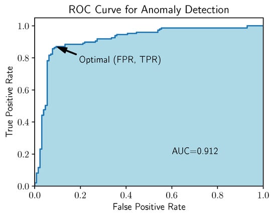
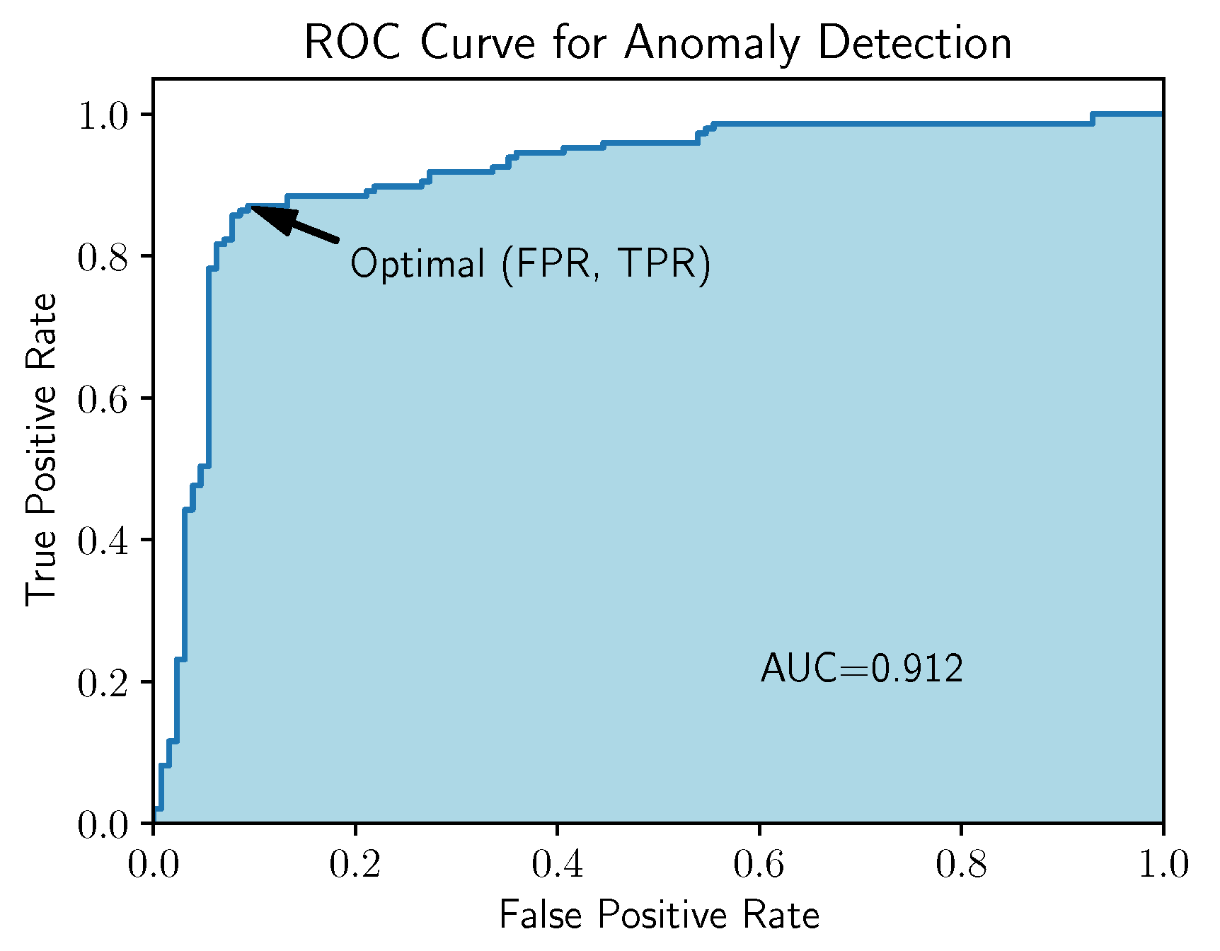
The idea of dynamic thresholding is not new [20,22]. The authors of [22] pointed out that the optimal threshold is the one corresponding to the upper left corner of the ROC curve, which is a good trade-off between low FPR and high TPR, as shown in Figure 4. While our method is also based on the ROC curve, it differs from the previous work in two aspects. First, our method uses only the anomaly scores of the reported instances and their verification results to construct the ROC curve, since the ground truths of all instances are not available due to selective verification. Second, anomaly detection tasks in different application scenarios may have different preferences in performance metrics; therefore, the dynamic thresholding algorithm in our scheme is configurable. The threshold actually used to determine whether an instance is an anomaly, ${\Theta }_{anom}$, is updated at run time by

$${\Theta }_{anom}=0.5+ϵ\times ({\Theta }_{roc}-0.5),$$

(3)

where ${\Theta }_{roc}$ is the optimal threshold computed from the ROC curve. The coefficient $ϵ(0\le ϵ\le 1)$ controls the trade-off between the default threshold (i.e., $0.5$) and ${\Theta }_{roc}$. Setting $ϵ$ to 0 is equivalent to disabling dynamic thresholding.

Figure 4. ROC curve and the optimal (FPR, TPR) that corresponds to the optimal threshold.

Note that dynamic thresholding does not utilize any information of future instances. Therefore, it can be integrated into a real-time anomaly detection scheme. The PADSV scheme with dynamic thresholding enabled is called PADSV-DT hereafter.

2.1.5. The Complete Algorithms

The PADSV scheme can be described by Algorithms 1 and 2. Algorithm 1 shows the steps of the offline prediction model training process, while Algorithm 2 shows the steps of the online anomaly detection process.

Algorithm 1: Offline model training.

Input: $\mathbf{S}$-historical sequence   Output: $\mathcal{M}$-prediction model   1 Construct and initialize an ED-CLA model, $\mathcal{M}$.   2 Convert $\mathbf{S}$ into a set of $({\mathbf{X}}_i,{\mathbf{y}}_i)$ pairs.   3 Split the set of $({\mathbf{X}}_i,{\mathbf{y}}_i)$ into a training set $S_{tr}$ and a test set $S_{te}$.   4 // Training:   5 for n epochs do   6       Feed each ${\mathbf{X}}_i$ in $S_{tr}$ to $\mathcal{M}$ to get the output ${\widehat{\mathbf{y}}}_i$.   7       Compute the mean squared error e between all ${\widehat{\mathbf{y}}}_i$’s and ${\mathbf{y}}_i$’s.   8       Back propagate e through the network of $\mathcal{M}$.   9 end 10 // Evaluation: 11 Feed each ${\mathbf{X}}_j$ in $S_{te}$ to $\mathcal{M}$ to get the output ${\widehat{\mathbf{y}}}_j$. 12 Compute the mean squared error between all ${\widehat{\mathbf{y}}}_j$’s and ${\mathbf{y}}_j$’s. 13 return $\mathcal{M}$

Algorithm 2: Online anomaly detection.

Input: $\mathcal{M}$-prediction model   1 Initialize the historical window, $\mathbf{W}$.   2 Initialize the Isolation Forest, $\mathcal{F}$.   3 Initialize the anomaly score threshold, ${\Theta }_{anom}=0.5$.   4 for every time point t do   5       Receive a new measurement, ${\mathbf{x}}_t$.   6       Feed $\mathbf{W}=({\mathbf{x}}_{t-T},{\mathbf{x}}_{t-T+1},\dots ,{\mathbf{x}}_{t-1})$ to $\mathcal{M}$ to generate ${\widehat{\mathbf{y}}}_t$.   7       Compute the residual ${\mathbf{r}}_t=|{\widehat{\mathbf{y}}}_t-{\mathbf{x}}_t|$.   8       Send ${\mathbf{r}}_t$ to $\mathcal{F}$ to get the anomaly score $s_t$.   9       if $s_t\ge {\Theta }_{anom}$ then 10            Send an alarm to the field engineers. 11            Receive and save the verification result. 12            if dynamic thresholding is enabled then 13                  Compute ROC using anomaly scores and verification results. 14                  Update ${\Theta }_{anom}$ based on ROC and Equation (3). 15            end 16       end 17       if verified and verification result is true anomaly then 18            Left-shift $\mathbf{W}$ and append ${\widehat{\mathbf{y}}}_t$ to it. 19       else 20            Left-shift $\mathbf{W}$ and append ${\mathbf{x}}_t$ to it. 21            Append ${\mathbf{x}}_t$ to the historical sequence, $\mathbf{S}$. 22       end 23 end

2.2. Self-Collected Datasets

The water quality data used to evaluate the proposed scheme were collected at three monitoring stations (Station A, B, and C) over an eight-year period (from January 2017 to May 2025). These monitoring stations were deployed by the Department of Ecology and Environment of Zhejiang Province, China in the water bodies around Hangzhou city. The stations measured five water quality parameters every four hours, i.e., pH, dissolved oxygen (DO), total phosphorus (TP), permanganate index (COD_Mn), and ammonia nitrogen (NH₃-N). As the capital of Zhejiang Province, Hangzhou has more than 12 million inhabitants and numerous industrial parks. It is very important to monitor the quality of water resources around the city.

There were many missing values and sporadic erroneous values in the collected time sequences. The missing instances accounted for 30–40% for each station (note: each instance contains five water quality parameter values). Since we had no information of anomalous events that might have occurred to the monitored water bodies during the collection time, we took common pre-processing steps to clean the data.

1.

We removed instances that were beyond sensor ranges, such as instances with pH values greater than 14, which were apparently caused by instrumental failures.

2.

We removed instances that were beyond a certain bound of “normal” data. More specifically, for each water quality parameter, for any instance x at time point t, we calculated the first quartile $Q_1$ and the third quartile $Q_3$ of instances between $t-15$ and $t+15$ (this is about a 5-day range given the measurement interval of 4 h). Then x was removed if $x<Q_1-1.5\times \mathrm{IQR}$ or $x>Q_3+1.5\times \mathrm{IQR}$ where $\mathrm{IQR}$ is the inter-quartile range, i.e., $\mathrm{IQR}=Q_3-Q_1$. The removal of x caused a missing instance at t.

3.

For each single-point missing instance, that is, the instance at t was missing but both instances at $t-1$ and $t+1$ were present, we filled the missing instance with the average value of the two adjacent instances.

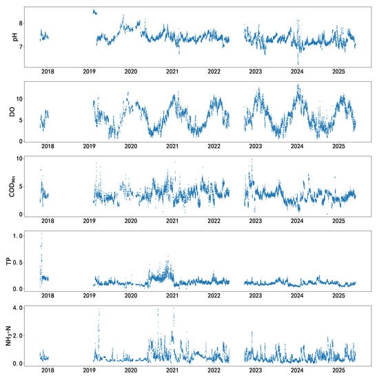
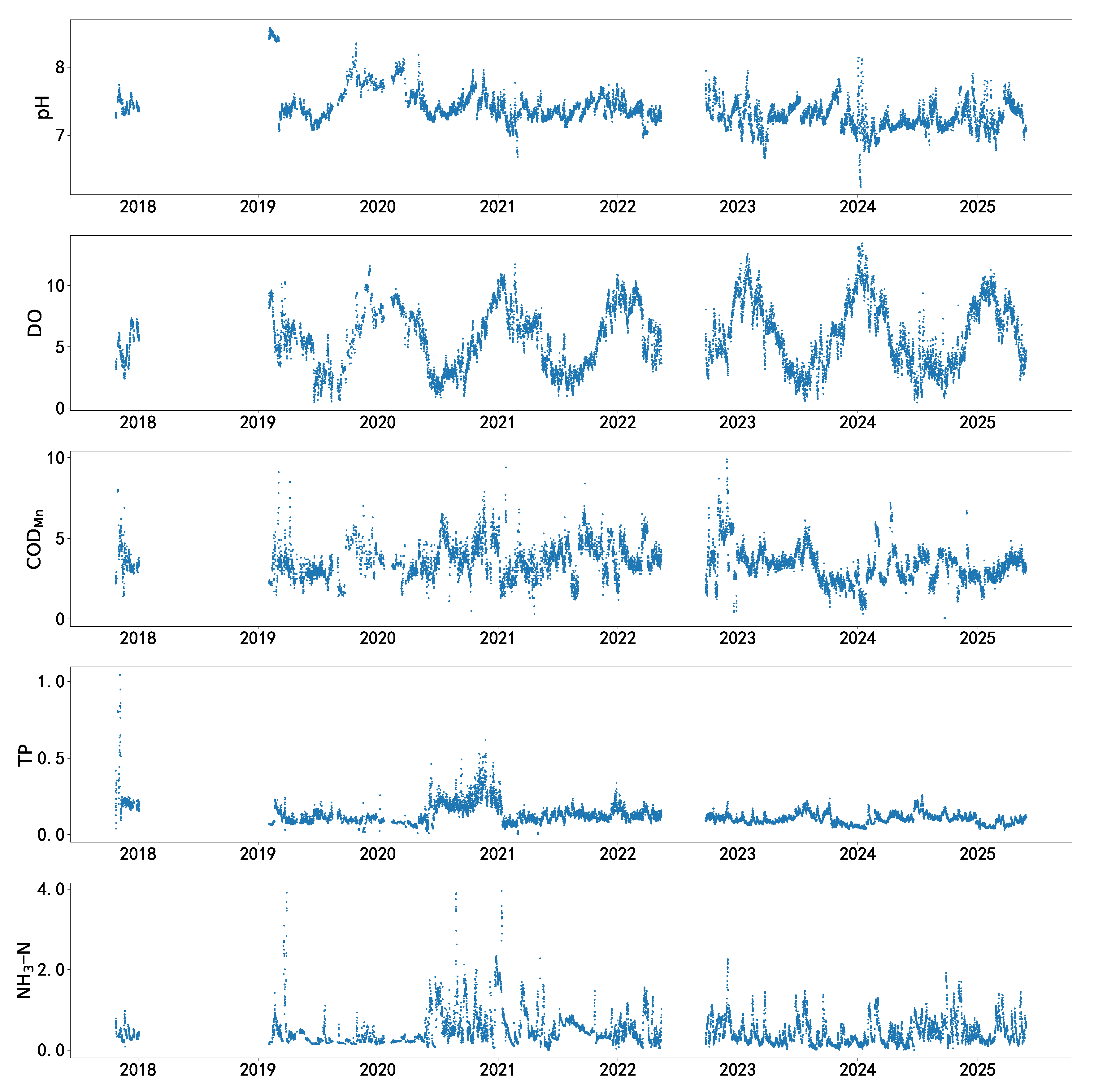
The data after these pre-processing steps were regarded as “normal” data, which, we assume, reflect the normal patterns of water quality at the specific monitoring station. Figure 5 shows the data from Station A after the above pre-processing steps. From the figure, we can see that (1) a lot of data are missing, especially those of 2017, 2018, and 2022; (2) while DO shows seasonal variation patterns, the other parameters have no explicit patterns, which makes it difficult for statistical approaches to make accurate predictions.

Figure 5. Data from Station A after pre-processing.

After pre-processing, the “normal” time sequence of each parameter from each station can be treated as a list of segments separated by missing values. Since we need a window of consecutive historical data, which has the size T, to predict the next value, segments not longer than T were discarded. Throughout our experiments, $T=24$, which corresponds to the result of grid search in our previous work [30].

Then the remaining instances from each station were divided into two sets, with the first 80% being prepared for prediction model training (known as training set), and the last 20% for prediction model testing and anomaly detection (known as test set). Finally, the training set were min-max normalized [35], and the minimum and maximum values of the training set before normalization were used to normalize the test set.

Anomaly Models

As aforementioned, the data from the three monitoring stations were cleaned and we assume that the resulting data were all normal measurements. In order to evaluate the proposed scheme, we manually added anomalies to each test set of the cleaned data.

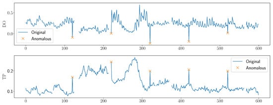
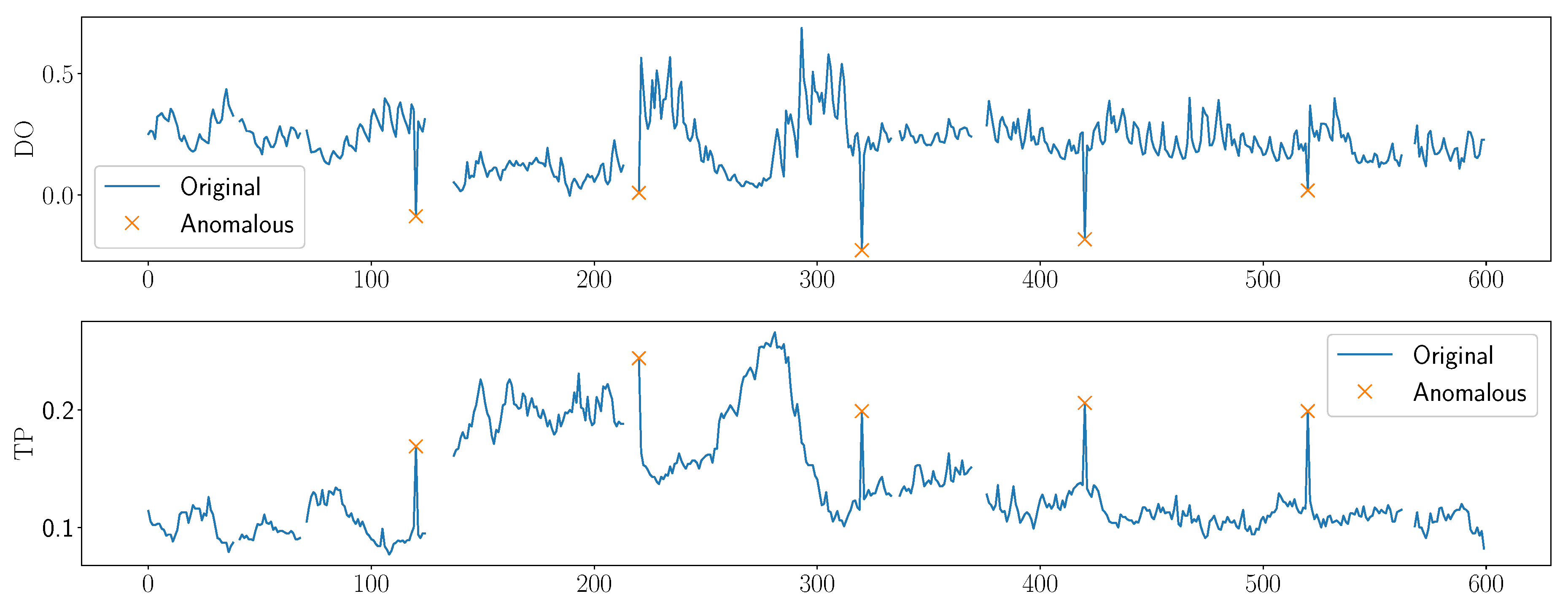
While there may be various types of anomalies in reality [36,37], in this study, we only simulated two types of anomalies, i.e., single-point anomalies and U-shaped (either upright or inverted) anomalies. A single-point anomaly is a measurement that is very different from those before and after it. Such anomalies are often results of technical failures in the monitoring devices. Though the anomalies are not related to water pollution, such failures should also be detected promptly, so that the devices can be fixed as soon as possible. Furthermore, successful detection of such events is crucial since we should not include these measurements in the history which is used to predict future values.

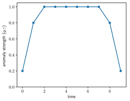
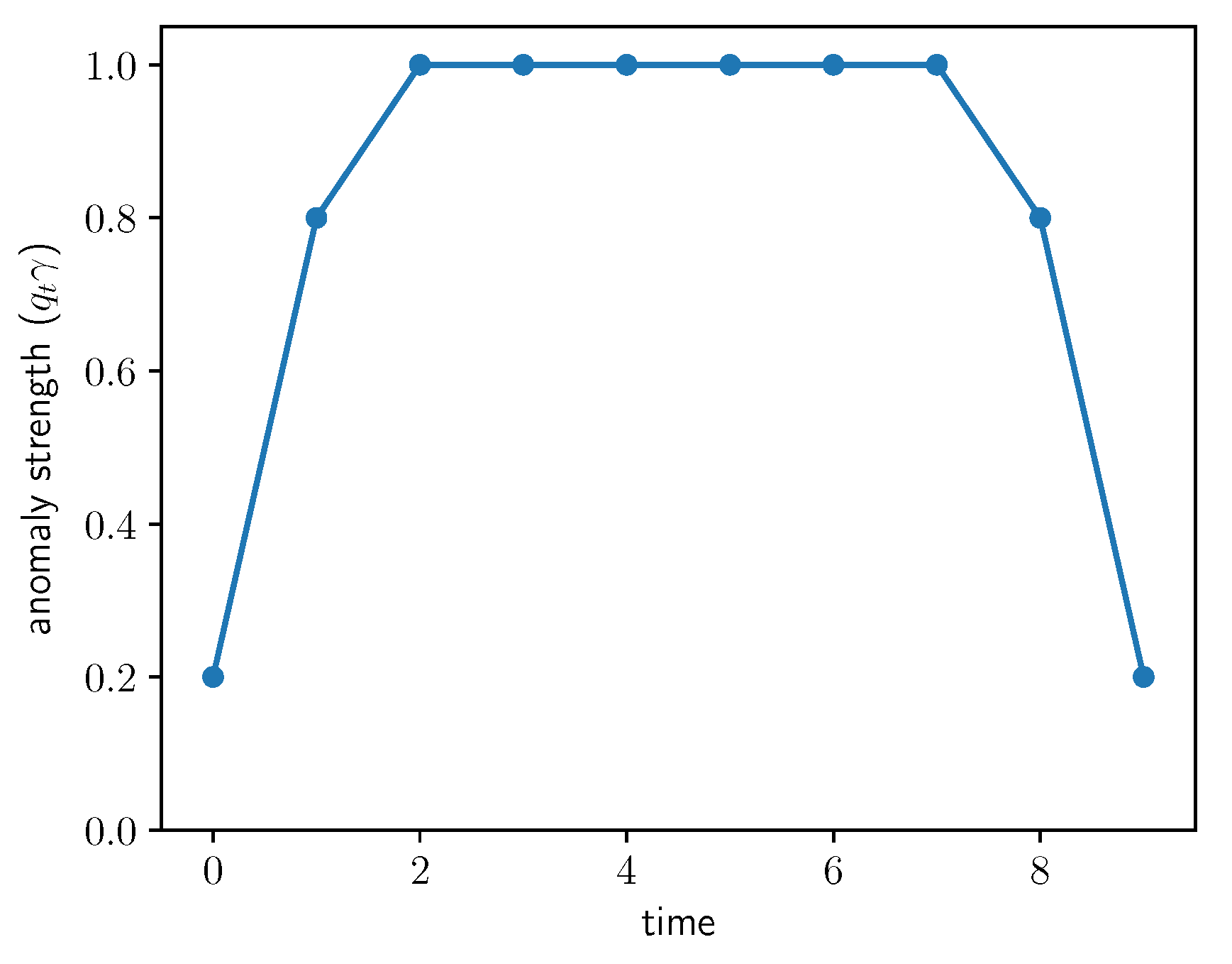
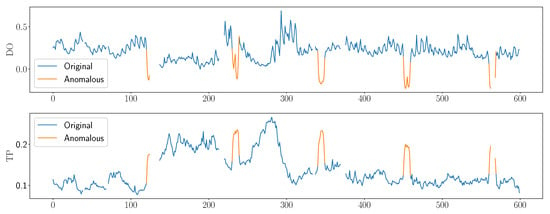
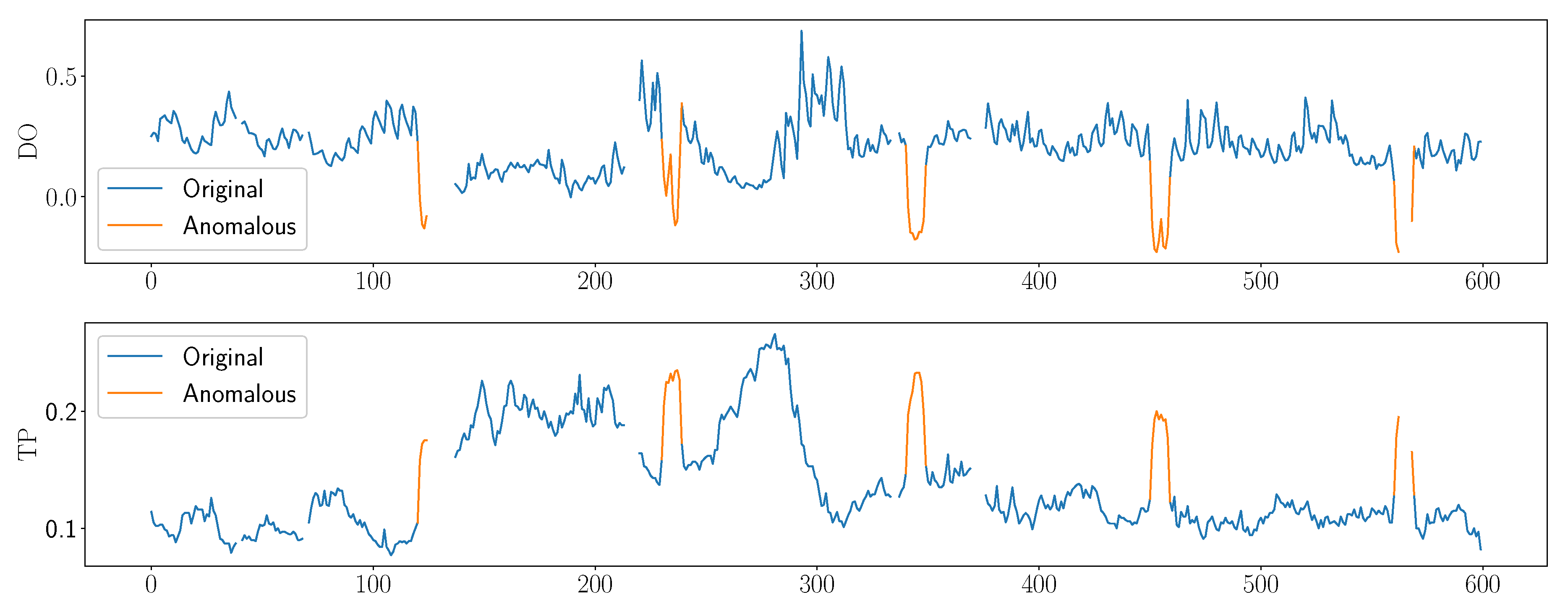
Inverted U-shaped anomalies have been widely used in water quality anomaly simulation [38]. Figure 6 shows an inverted U-shaped model, which is a burst of 10 time units of anomalies that can be superimposed to the original time sequence. The strength of the anomalies, denoted by the product of $\mathbf{q}$ and $\gamma$, rises at the first two time units in the burst until it reaches the plateau, and decreases at the last two time units. The anomaly intensity, $\gamma$, is a hyperparameter that adjusts the overall strength of the anomalies in the burst, while $\mathbf{q}$ is a vector of coefficients to vary the strength of each anomaly in the burst; in Figure 6, $\mathbf{q}=(q_0,q_1,\dots ,q_9)=(0.2,0.8,1.0,1.0,1.0,1.0,1.0,1.0,0.8,0.2)$. Such models are a simplification of the usual patterns of anomaly bursts in reality.

Figure 6. An inverted U-shaped anomaly model ($\gamma =1.0$).

If such a burst of anomalies is superimposed to a time sequence $\mathbf{X}=({\mathbf{x}}_0,{\mathbf{x}}_1,\dots ,{\mathbf{x}}_t,\dots )$ at time t, then the values in the time sequence between t (inclusive) and $t+10$ (exclusive) are updated by

$${\mathbf{x}}_{t+i}^{\prime }={\mathbf{x}}_{t+i}+q_i\times \gamma \times {\sigma }_{\mathbf{x}},$$

(4)

where ${\sigma }_{\mathbf{x}}$ is the standard deviation of the original sequence $\mathbf{X}$, and $0\le i\le 9$. Replace the + sign in Equation (4) with a − sign to apply an upright U-shaped anomaly model (whether it is upright U-shaped or inverted U-shaped makes no difference in a prediction-based anomaly detection scheme; therefore, both models are referred to as the U-shaped model hereafter unless otherwise stated). Multiple bursts of anomalies can be superimposed to the original time sequence. It is easily seen that a single-point anomaly is a special case of the U-shaped anomaly with $\mathbf{q}$ containing only one coefficient $1.0$.

Figure 7 and Figure 8 each show an example of single-point anomalies and U-shaped anomalies, respectively, added to the originally normal DO and TP sequences (originally missing values were excluded from anomaly superimposition). Since pollution events usually cause the DO amount in the water to decrease and TP to increase, in these examples, we applied downward single-point and upright U-shaped anomalies to DO, and upward single-point and inverted U-shaped anomalies to TP.

Figure 7. An example of single-point anomalies ($\gamma =2.0$).

Figure 8. An example of U-shaped anomalies ($\gamma =2.0$).

2.3. Public Dataset: GECCO2018

The GECCO2018 dataset [39] is a real-world water quality time sequence with every instance in the sequence clearly labeled as normal or anomalous. In addition to the values of water quality parameters, the dataset also contains columns that are not directly related to water quality, such as temperature and flow rate. In our experiments, we focused on the water quality parameters only, which are shown in Table 1.

Table 1. Water quality parameters in the GECCO2018 dataset.

Column	Description
pH	pH value
Redox	Redox potential, measured in mV
EC	Electric conductivity, measured in μS/cm
Turb	Turbidity, measured in NTU
Cl	Amount of chlorine dioxide, measured in mg/L (MS1)
Cl_2	Amount of chlorine dioxide, measured in mg/L (MS2)

The dataset contains 139,566 instances, among which 1726 are anomalies (1.24% of the total). Since the first 16,000 instances are all normal ones, we used them as the training set, and the remaining instances as the test set.

2.4. Evaluation Methodology

This section describes the metrics and experimental settings that were used to evaluate the proposed scheme.

2.4.1. Performance Metrics

The result of anomaly detection for one particular instance is one of the following:

• True Positive: An actual anomaly is correctly detected as anomalous.
• True Negative: A normal instance is correctly detected as normal.
• False Positive: A normal instance is incorrectly detected as anomalous.
• False Negative: An actual anomaly is incorrectly detected as normal.

Accuracy measures the overall detection performance and is defined as

$$\mathrm{Accuracy}={\displaystyle \frac{\mathrm{TP}+\mathrm{TN}}{\mathrm{TP}+\mathrm{TN}+\mathrm{FP}+\mathrm{FN}}},$$

(5)

where $\mathrm{TP}$, $\mathrm{TN}$, $\mathrm{FP}$, and $\mathrm{FN}$ are the numbers of true positives, true negatives, false positives, and false negatives, respectively.

However, for imbalanced data, which are commonly seen in anomaly detection tasks [27,28,40], precision and recall are used more often than accuracy. They are defined as

$$\mathrm{Precision}={\displaystyle \frac{\mathrm{TP}}{\mathrm{TP}+\mathrm{FP}}}$$

(6)

and

$$\mathrm{Recall}=\mathrm{TPR}={\displaystyle \frac{\mathrm{TP}}{\mathrm{TP}+\mathrm{FN}}}.$$

(7)

Note: Recall is the same as the True Positive Rate (TPR).

In PADSV, each detected anomaly is reported (in the form of an alarm) to field engineers for verification, which induces a certain amount of labor cost. The false alarm rate (i.e., False Positive Rate, FPR) measures the labor efficiency of the scheme, which is defined as

$$\mathrm{FPR}={\displaystyle \frac{\mathrm{FP}}{\mathrm{FP}+\mathrm{TN}}}.$$

(8)

Note that the TPR and FPR computed in evaluation are different from those computed in dynamic thresholding. In evaluation, the TPR and FPR are computed based on the detection results and the ground truths of all instances in the entire test set. In dynamic thresholding, the TPR and FPR are computed based on the detection results and the verification results of the reported instances only. The true labels of unreported instances are unknown to the detection scheme at run time.

As a prediction-based scheme, accurate anomaly detection highly relies on the accurate prediction of future values. Prediction accuracy is often measured by Root Mean Square Error (RMSE) and Nash–Sutcliffe Efficiency (NSE) [41]. RMSE measures the errors between the predicted values and the observed (i.e., true) values, while NSE measures how well the predicted values match the true values. Thus, an RMSE close to zero and an NSE close to 1 indicate good prediction performance. The two metrics are defined as

$$\mathrm{RMSE}=\sqrt{{\displaystyle \frac{1}{N}}{\displaystyle \sum _{i=1}^N}{(y_i-{\widehat{y}}_i)}^2}$$

(9)

and

$$\mathrm{NSE}=1-{\displaystyle \frac{{\sum }_{i=1}^N{({\widehat{y}}_i-y_i)}^2}{{\sum }_{i=1}^N{(y_i-\overline{y})}^2}},$$

(10)

where ${\widehat{y}}_i$ represents a predicted value, $y_i$ represents the corresponding true value, $\overline{y}$ represents the mean of the true values, and N is the total number of predictions.

2.4.2. Experimental Settings

While the idea of prediction-based anomaly detection has been widely investigated in the existing research, most of such work focuses on the improvement of algorithms, and lacks implementation details for real-time deployment. For comparison purposes, we constructed two reference schemes, ${\mathcal{S}}_0$ and ${\mathcal{S}}_1$, that are similar to existing ones to some degree. Additionally, we chose a more general-purpose algorithm called USAD [13], which is one of the state-of-the-art anomaly detection algorithms designed for all types of time sequences, as another reference scheme. They are briefly described as follows.

• ${\mathcal{S}}_0$: In this scheme, alarms are sent to field engineers; however, the scheme does not expect or utilize the verification results from the engineers. The scheme solely depends on the built-in anomaly detection capability of the Isolation Forest algorithm to detect anomalies. The actual measurements in the historical window are never replaced by predicted values in spite of the detection results. ${\mathcal{S}}_0$ represents the class of prediction-based anomaly detection schemes that does not consider verification.
• ${\mathcal{S}}_1$: In this scheme, every detection result is reported to the field engineers, and every verification result is utilized. For confirmed anomalies, corresponding measurements are replaced by predicted values. ${\mathcal{S}}_1$ represents the class of prediction-based anomaly detection schemes that assumes the ground truths of all instances are known. While this scheme is certainly labor inefficient, it provides a reference for the proposed PADSV scheme in which verification is selective.
• USAD: USAD is an unsupervised anomaly detection algorithm for multivariate time sequences. The detection model is trained with normal sequential data, sliced into a set of small windows. When running in the inference mode, the detection model also receives the data in the form of windows. The model assigns an anomaly score to each window, depending on how much the window deviates from the windows used in training, and raises an alarm if the score exceeds the threshold. Due to the design of USAD, its deployment in our experiments differed from the other schemes in two significant ways.

  1.

  Detection results from USAD were evaluated on per-window basis rather than on per-time point basis. For each window that was detected as anomalous, if the window did contain an actual anomaly, despite the location of the anomaly in the window, the result was regarded as a true positive.

  2.

  The algorithm did not provide a default threshold. The anomaly scores and the ground truths of all test windows were used to find the optimal threshold, following the ROC-based method similar to that discussed in Section 2.1.4. Then the threshold was used to determine anomalies. Therefore, the performance we got from USAD was its upper bound; had we chosen a sub-optimal threshold (since in reality we might not be able to learn the ground truths of all windows and thus would not be able to compute the optimal threshold), the performance would have been worse than reported.

The USAD implementation was based on https://github.com/manigalati/usad (accessed on 26 February 2026). Hyperparameters of the prediction model of PADSV were set to the default as in [30], which were the result of the grid search in the previous work. For Isolation Forests, we adopted the default parameters as defined in scikit-learn (https://scikit-learn.org (accessed on 19 September 2025)). The code of PADSV, ${\mathcal{S}}_0$ and ${\mathcal{S}}_1$ can be found at https://github.com/eastlakesoft/anomaly-detect-pub (accessed on 15 March 2026). The experiments were run on a desktop computer equipped with an Intel 2.50 GHz CPU and 16 GB memory.

3. Results

We evaluated the performance of PADSV and PADSV-DT (with $ϵ=0.5$ unless stated otherwise), as well as the reference schemes, through extensive experiments using the data collected from the monitoring stations and the GECCO2018 dataset. The results are reported in this section.

3.1. Prediction Accuracy

Table 2 shows the RMSEs and NSEs of the prediction on the original test data (after min-max normalization but before anomaly superimposition) for all of the three monitoring stations. From the table, we can see that most of the RMSEs are between 0.01 and 0.04, which seem to be small for the normalized data. However, since the normalization of the test data was based on the minimum and maximum values of the training data, unlike the training data, the normalized test data may not be bounded by zero and one. Therefore, we should also check the NSEs, which indicate how the predicted values match the true values (i.e., measurements). Table 2 shows that the NSEs for DO, TP, and NH₃-N of Station A are all over 0.9, and NSEs for pH and COD_Mn are close to 0.8. As shown in Figure 5, the pH and COD_Mn curves of Station A contain fewer regular patterns than the other three water quality parameters, making them more difficult to predict. The NSEs for DO of all three stations are above 0.95, indicating high prediction accuracy for this parameter, as we expected since it has the most regular variation pattern among all of the five water quality parameters.

Table 2. RMSEs and NSEs of the prediction on the original test data.

Station		pH	DO	CODMn	TP	NH3-N
A	RMSE	0.0349	0.0407	0.0359	0.0097	0.0222
	NSE	0.8076	0.9573	0.7904	0.9415	0.9277
B	RMSE	0.0268	0.0394	0.0330	0.0088	0.0232
	NSE	0.9360	0.9650	0.7986	0.8212	0.9484
C	RMSE	0.0292	0.0243	0.0355	0.0106	0.0346
	NSE	0.9491	0.9881	0.7553	0.7899	0.8707

In reality, the measurements from monitoring stations may be mixed with anomalies. According to our design, when PADSV detects an anomaly and receives confirmation from the field engineers, it replaces the anomalous measurement with the predicted value in the historical window, preventing the anomaly from “contaminating” the intrinsic patterns of the normal data. Thus, if the subsequent measurements are still anomalous, the corresponding residuals will remain large and prone to detection.

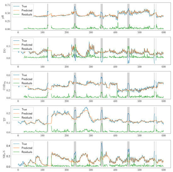
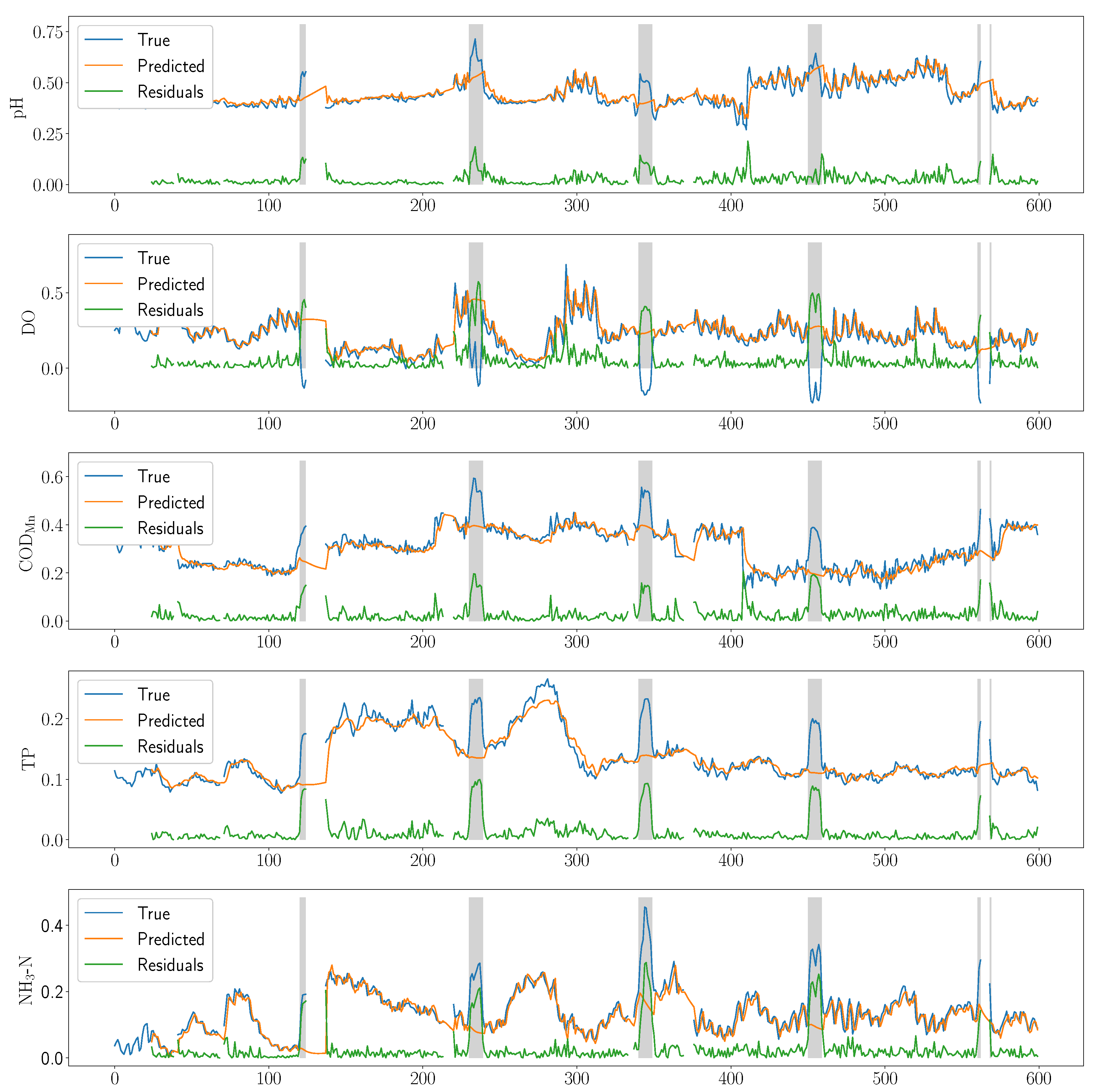
The effectiveness of this design is illustrated in Figure 9, which shows the prediction results on the test data from Station A. The measurements of all five water quality parameters were superimposed with periodic U-shaped anomalies with intensity $\gamma =2.0$, following the approach depicted in Section 2.2. For clarity, only data at the first 600 time points are shown, indexed by integers instead of dates and times. The gray bars in the figure indicate when the anomalies occurred. We can see that normally the predicted values closely matched the measurements, resulting in small residuals. During each anomaly burst, the actual measurements significantly deviated from the normal values, while the prediction still followed the previous trend, resulting in large residuals, which would trigger successive alarms.

Figure 9. Predicted values and residuals as the intermediate outcome of PADSV ($\gamma =2.0$) (gray bars: actual anomaly bursts).

Moreover, at the time points where the measurements were missing (such as $127\le t\le 138$ in Figure 9), the prediction model was still able to make predictions based on the previous data (either measurements or previously predicted values), although the residuals could not be computed.

For comparison, Figure 10 shows the prediction results of TP from the ${\mathcal{S}}_0$ scheme using the same test data. Since ${\mathcal{S}}_0$ employed no verification and correction, the prediction was highly impacted by the anomalous measurements. From the figure, we can see abrupt rises in prediction residuals at both edges of an anomaly burst. However, the residuals were small in the middle of the burst. Therefore, if the detection process had missed the signals at the beginning of an anomaly burst, it would be very likely that the pollution event remained undiscovered until the end when it might be too late to prevent the event from causing serious damage.

Figure 10. Predicted values and residuals as the intermediate outcome of ${\mathcal{S}}_0$ ($\gamma =2.0$) (gray bars: actual anomaly bursts).

3.2. Performance of Anomaly Detection in Various Anomaly Scenarios

In reality, a pollution event may affect the values of one or more water quality parameters, or one or more sensors in a monitoring station may go wrong. Therefore, we experimented with PADSV and the other schemes in different scenarios in which measurements of one, three, or all of the five water quality parameters contained either single-point or U-shaped anomalies. For convenience of description, these scenarios are denoted by SpA-i and UsA-i hereafter, where SpA stands for single-point anomalies and UsA for U-shaped anomalies, and $i=1,3,5$ is the number of anomalous water quality parameters in a scenario. In the SpA-1 and UsA-1 scenarios, only one water quality parameter was anomalous, which could be any one of pH, DO, TP, COD_Mn, and NH₃-N; thus, we ran experiments with each possibility and averaged the performance metrics over the multiple runs. The SpA-3 and UsA-3 scenarios were processed in the same way. For the SpA-5 and UsA-5 scenarios, we ran the same experiment multiple times, each time with a different random seed, and then averaged the performance metrics.

We also evaluated the schemes under various anomaly intensities. While extensive experiments were run for test data from all three monitoring stations, to save space, only the results of Station A are shown. the results of the other stations are similar to those of Station A.

3.2.1. On Test Data with Single-Point Anomalies

Table 3 lists the average performance of the five schemes on the test data with single-point anomalies added to one, three, or all five water quality parameters, respectively.

Table 3. Anomaly detection performance on test data with single-point anomalies (±half of the confidence interval at the 95% confidence level; values less than 0.005 are shown as 0.00. USAD was run only once for each SpA-5 scenario due to lack of randomization in the inference mode).

		SpA-1			SpA-3			SpA-5
$\gamma$	Scheme	Precision	Recall	FPR	Precision	Recall	FPR	Precision	Recall	FPR
1.0	USAD	0.09 ± 0.00	0.46 ± 0.01	0.54 ± 0.01	0.09 ± 0.00	0.47 ± 0.01	0.53 ± 0.01	0.10	0.48	0.51
	${\mathcal{S}}_0$	0.05 ± 0.03	0.69 ± 0.38	0.11 ± 0.00	0.08 ± 0.00	1.00 ± 0.00	0.10 ± 0.00	0.08 ± 0.00	1.00 ± 0.00	0.10 ± 0.00
	${\mathcal{S}}_1$	0.05 ± 0.03	0.70 ± 0.42	0.10 ± 0.00	0.08 ± 0.00	1.00 ± 0.00	0.10 ± 0.00	0.08 ± 0.00	1.00 ± 0.00	0.10 ± 0.00
	PADSV	0.05 ± 0.03	0.70 ± 0.39	0.10 ± 0.00	0.08 ± 0.00	0.99 ± 0.01	0.10 ± 0.00	0.08 ± 0.00	1.00 ± 0.00	0.10 ± 0.00
	PADSV-DT	0.06 ± 0.03	0.39 ± 0.33	0.05 ± 0.02	0.15 ± 0.02	0.98 ± 0.03	0.05 ± 0.01	0.21 ± 0.01	1.00 ± 0.00	0.03 ± 0.00
2.0	USAD	0.10 ± 0.03	0.48 ± 0.08	0.50 ± 0.08	0.13 ± 0.02	0.55 ± 0.05	0.44 ± 0.05	0.17	0.62	0.37
	${\mathcal{S}}_0$	0.08 ± 0.00	1.00 ± 0.00	0.10 ± 0.01	0.08 ± 0.00	1.00 ± 0.00	0.09 ± 0.00	0.08 ± 0.00	1.00 ± 0.00	0.09 ± 0.00
	${\mathcal{S}}_1$	0.08 ± 0.01	0.99 ± 0.03	0.10 ± 0.01	0.09 ± 0.00	1.00 ± 0.00	0.09 ± 0.00	0.09 ± 0.00	1.00 ± 0.00	0.09 ± 0.00
	PADSV	0.08 ± 0.01	0.97 ± 0.09	0.10 ± 0.00	0.09 ± 0.00	1.00 ± 0.00	0.09 ± 0.00	0.09 ± 0.00	1.00 ± 0.00	0.09 ± 0.00
	PADSV-DT	0.12 ± 0.03	0.89 ± 0.20	0.06 ± 0.01	0.25 ± 0.01	1.00 ± 0.00	0.02 ± 0.00	0.30 ± 0.01	1.00 ± 0.00	0.02 ± 0.00
3.0	USAD	0.13 ± 0.08	0.52 ± 0.15	0.47 ± 0.14	0.20 ± 0.06	0.64 ± 0.09	0.35 ± 0.09	0.29	0.76	0.23
	${\mathcal{S}}_0$	0.08 ± 0.01	1.00 ± 0.00	0.09 ± 0.01	0.09 ± 0.00	1.00 ± 0.00	0.09 ± 0.00	0.09 ± 0.00	1.00 ± 0.00	0.08 ± 0.00
	${\mathcal{S}}_1$	0.08 ± 0.01	1.00 ± 0.00	0.09 ± 0.01	0.09 ± 0.00	1.00 ± 0.00	0.08 ± 0.00	0.09 ± 0.00	1.00 ± 0.00	0.08 ± 0.00
	PADSV	0.08 ± 0.00	1.00 ± 0.00	0.09 ± 0.00	0.09 ± 0.00	1.00 ± 0.00	0.08 ± 0.00	0.09 ± 0.00	1.00 ± 0.00	0.08 ± 0.00
	PADSV-DT	0.14 ± 0.02	0.98 ± 0.06	0.05 ± 0.01	0.30 ± 0.01	1.00 ± 0.00	0.02 ± 0.00	0.34 ± 0.02	1.00 ± 0.00	0.02 ± 0.00

From Table 3, we can see that in the scenario of SpA-1 with $\gamma =1.0$, all of the five schemes reported a very low precision, meaning that most of the detected anomalous instances were actually normal ones. Given the low anomaly intensity and as few as one anomalous water quality parameter, it is not beyond our expectation that all of these schemes showed poor performance. The recall of ${\mathcal{S}}_0$ was close to those of ${\mathcal{S}}_1$ and PADSV, since in scenarios with single-point anomalies that were separated by long intervals, the occurrence of one anomaly would not affect the detection of later anomalies even without verification of the former one. Regarding false alarms, USAD reported a very high FPR. The FPRs of ${\mathcal{S}}_0$, ${\mathcal{S}}_1$ and PADSV were close, with that of ${\mathcal{S}}_0$ slightly higher since without verification, the occurrence of one anomaly would more likely make the prediction of the next instance deviate from the normal value, leading to a false positive.

On the other hand, by dynamically adjusting the anomaly threshold, PADSV-DT significantly reduced FPR by almost 50% compared with PADSV, at the cost of a lower recall. As we have discussed in Section 2.1.4, PADSV-DT attempts to hit the balance between TPR and FPR based on the verification results, and accordingly, the experiments showed that it achieved a higher accuracy than PADSV. Therefore, if accuracy is the top priority in an anomaly detection task, PADSV-DT is a better option than PADSV.

When there were more anomalous water quality parameters (from left to right in Table 3), all of the five schemes reported higher precision and recall rates as well as lower FPRs, since with more anomalous attributes, anomalous instances were easier to separate from normal instances. The trend was also true when the anomaly intensity increased (from top to bottom in Table 3), as anomalies were easier to detect when they were more outstanding. Yet the trend was not so notable for USAD as for the other schemes. Since all of the other schemes are prediction-based, the difference in the trend indicates the advantage of using prediction-based approaches in water quality anomaly detection.

In all scenarios, PADSV showed very similar precision, recall, and FPRs compared with ${\mathcal{S}}_1$. While they both enforce verification, ${\mathcal{S}}_1$ requires verification of every instance, which demands unrealistically high labor costs. PADSV, on the other hand, only requests verification for instances that are detected positive, which makes it a realistic solution to anomaly detection problems.

Table 3 also lists the confidence intervals at the 95% confidence level for each performance value. The confidence intervals from the SpA-1, $\gamma =1.0$ scenario, especially those of the recall rates of the four prediction-based schemes, were unacceptably large, due to two reasons: first, the low anomaly intensity made it difficult for the schemes to detect all anomalies; second, as we have seen, different water parameters exhibited different levels of regularity, causing large variations in detection performance. However, with the increase in anomaly intensity or the number of anomalous water parameters, the performance became more consistent across multiple runs.

3.2.2. On Test Data with U-Shaped Anomalies

Table 4 lists the average performance of the five schemes on the test data with U-shaped anomalies added to one, three, or all five water quality parameters, respectively. It can be seen that USAD had the highest FPR among the five schemes in all scenarios, yet its precision and recall were not higher than the others. Among the four prediction-based schemes, ${\mathcal{S}}_0$ achieved the lowest precision and recall and the highest FPR in almost all scenarios. PADSV and ${\mathcal{S}}_1$ had comparable precision, recall, and FPR, especially in the scenarios where there were more anomalous water quality parameters. In the scenario of UsA-5 and $\gamma =1.0$, the precision and recall rates of PADSV were almost twice as high as those of ${\mathcal{S}}_0$, while the FPR was 20% lower, showing a significant improvement in performance by utilizing human verification in anomaly detection.

Table 4. Anomaly detection performance on test data with U-shaped anomalies (±half of the confidence interval at the 95% confidence level; values less than 0.005 are shown as 0.00. USAD was run only once for each UsA-5 scenario due to lack of randomization in the inference mode).

		UsA-1			UsA-3			UsA-5
$\gamma$	Scheme	Precision	Recall	FPR	Precision	Recall	FPR	Precision	Recall	FPR
1.0	USAD	0.13 ± 0.01	0.42 ± 0.02	0.57 ± 0.03	0.14 ± 0.01	0.44 ± 0.02	0.55 ± 0.02	0.16	0.47	0.53
	${\mathcal{S}}_0$	0.13 ± 0.04	0.22 ± 0.08	0.11 ± 0.00	0.22 ± 0.01	0.40 ± 0.04	0.11 ± 0.00	0.23 ± 0.01	0.43 ± 0.01	0.11 ± 0.00
	${\mathcal{S}}_1$	0.31 ± 0.07	0.55 ± 0.14	0.09 ± 0.01	0.43 ± 0.02	0.83 ± 0.03	0.08 ± 0.00	0.44 ± 0.01	0.86 ± 0.01	0.08 ± 0.00
	PADSV	0.21 ± 0.08	0.34 ± 0.17	0.09 ± 0.01	0.38 ± 0.03	0.71 ± 0.07	0.09 ± 0.00	0.44 ± 0.01	0.87 ± 0.01	0.08 ± 0.00
	PADSV-DT	0.21 ± 0.09	0.24 ± 0.12	0.06 ± 0.01	0.36 ± 0.03	0.45 ± 0.06	0.06 ± 0.00	0.50 ± 0.02	0.69 ± 0.06	0.05 ± 0.00
2.0	USAD	0.17 ± 0.07	0.48 ± 0.11	0.52 ± 0.11	0.25 ± 0.05	0.60 ± 0.06	0.39 ± 0.06	0.33	0.70	0.30
	${\mathcal{S}}_0$	0.22 ± 0.11	0.40 ± 0.26	0.10 ± 0.00	0.32 ± 0.04	0.62 ± 0.09	0.09 ± 0.00	0.34 ± 0.01	0.64 ± 0.02	0.09 ± 0.00
	${\mathcal{S}}_1$	0.41 ± 0.05	0.79 ± 0.09	0.08 ± 0.01	0.47 ± 0.01	0.89 ± 0.01	0.07 ± 0.00	0.49 ± 0.01	0.92 ± 0.00	0.07 ± 0.00
	PADSV	0.33 ± 0.09	0.58 ± 0.19	0.09 ± 0.01	0.47 ± 0.01	0.88 ± 0.01	0.07 ± 0.00	0.48 ± 0.01	0.92 ± 0.01	0.07 ± 0.00
	PADSV-DT	0.32 ± 0.12	0.40 ± 0.23	0.06 ± 0.01	0.61 ± 0.02	0.84 ± 0.01	0.04 ± 0.00	0.65 ± 0.01	0.85 ± 0.01	0.03 ± 0.00
3.0	USAD	0.22 ± 0.15	0.55 ± 0.16	0.44 ± 0.18	0.39 ± 0.07	0.74 ± 0.06	0.26 ± 0.06	0.49	0.82	0.18
	${\mathcal{S}}_0$	0.28 ± 0.12	0.50 ± 0.29	0.09 ± 0.01	0.39 ± 0.05	0.76 ± 0.12	0.09 ± 0.00	0.44 ± 0.01	0.90 ± 0.01	0.09 ± 0.00
	${\mathcal{S}}_1$	0.45 ± 0.03	0.88 ± 0.03	0.08 ± 0.01	0.50 ± 0.01	0.93 ± 0.02	0.07 ± 0.00	0.52 ± 0.01	0.97 ± 0.01	0.07 ± 0.00
	PADSV	0.41 ± 0.07	0.74 ± 0.12	0.08 ± 0.01	0.50 ± 0.01	0.92 ± 0.02	0.07 ± 0.00	0.52 ± 0.01	0.97 ± 0.01	0.07 ± 0.00
	PADSV-DT	0.39 ± 0.12	0.50 ± 0.22	0.06 ± 0.01	0.66 ± 0.01	0.85 ± 0.01	0.03 ± 0.00	0.67 ± 0.01	0.90 ± 0.00	0.03 ± 0.00

Similar to the cases of single-point anomalies, PADSV-DT always had the lowest FPR, boosting accuracy at the cost of recall (i.e., having more detection misses). For each scheme, the precision and recall increased with the anomaly intensity and the number of anomalous water quality parameters, and the FPR decreased in the meantime, indicating better detection performance.

From Table 3, we can see that in some SpA scenarios, the recall of most schemes became 1.0, meaning that all anomalies were captured. However, in the scenarios with U-shaped anomalies, none of the five schemes achieved a recall of 1.0. In each scenario, there were some anomalies that had eluded detection, though the number of such anomalies became smaller when $\gamma$ or the number of anomalous parameters became larger. This is because a U-shaped anomaly burst differs from a single-point one in that it gradually deviates from the normal trend at the beginning of the burst and gradually returns to the normal trend in the end. Therefore, it is difficult to capture the anomalies at the two ends of a U-shaped burst, where the prediction residuals are small. Once the prediction residual is large enough to flag an anomaly, PADSV keeps prediction on the normal track with the help of verification, maintaining large prediction residuals during the burst. In ${\mathcal{S}}_0$, where no verification is utilized, prediction is distorted by the anomalous data, yielding small prediction residuals in the middle of the burst and causing many detection misses, as validated by Figure 10 and the recall rates in Table 4.

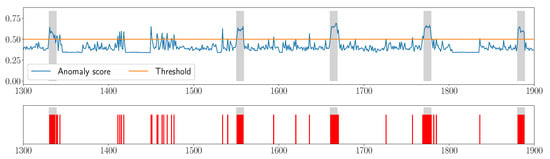
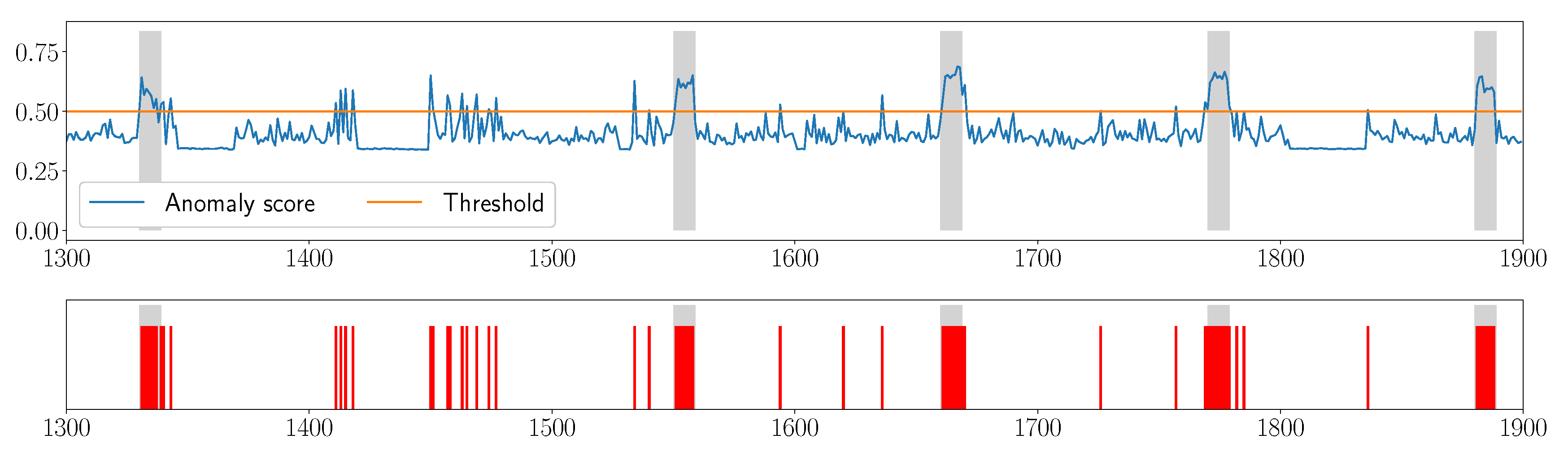
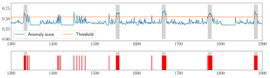
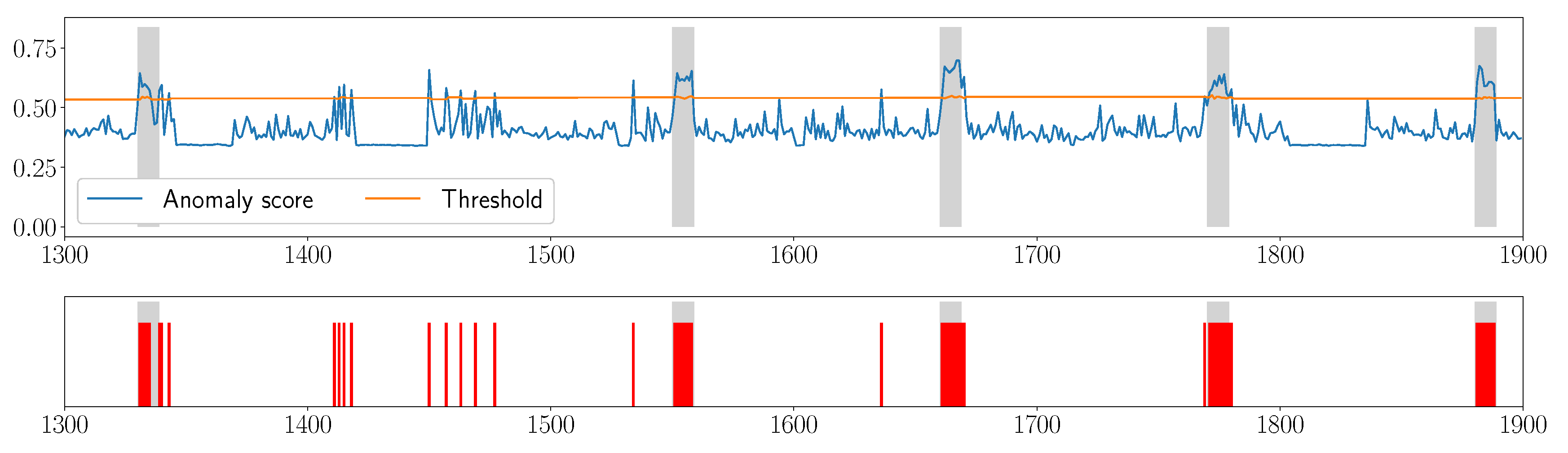
Figure 11 shows the anomaly scores calculated and alarms sent by PADSV on the test data in a run of the UsA-5 scenario with $\gamma =1.0$. In addition to anomaly scores, the top plot also shows the anomaly threshold, which remained constant (i.e., 0.5) per the design of PADSV. Instances with prediction residuals’ anomaly scores above the threshold were reported as anomalies and alarms were sent to the field engineers for verification. From the bottom plot, we see that all of the five displayed anomaly bursts were detected by PADSV, though the scheme missed a few anomalies at the beginning of most bursts. The scheme also sent a few false alarms. Since the anomaly intensity $\gamma$ was as low as 1.0, the anomalous data were not very outstanding compared with the normal ones, and some bumpy normal data were regarded as anomalies by PADSV.

Figure 11. Anomaly scores, thresholds, and sent alarms of PADSV in UsA-5 with $\gamma =1.0$ (gray bars: actual anomaly bursts; red bars: alarms).

Dynamically adjusting the threshold based on the field engineers’ verification can reduce these false alarms, as illustrated in Figure 12. Meanwhile, the PADSV-DT scheme missed more anomalies than PADSV, especially those not so prominent such as those in the first burst in the plot. However, the scheme did capture all of the anomaly bursts. If the requirement is that at least one alarm is raised for each anomaly burst, then PADSV-DT is a good trade-off between coverage and cost.

Figure 12. Anomaly scores, thresholds, and sent alarms of PADSV-DT ($ϵ=0.5$) in UsA-5 with $\gamma =1.0$ (gray bars: actual anomaly bursts; red bars: alarms).

3.3. Effect of Reporting Selectivity

The parameter $ϵ$ controls the reporting selectivity in the PADSV-DT scheme. When $ϵ=1.0$, the threshold returned from the ROC-based adjustment (which is always greater than or equal to 0.5, since the initial threshold that the scheme starts with is 0.5) is used to determine whether a prediction residual indicates an anomaly. When $ϵ=0$, the constant threshold 0.5 is used instead, just like how PADSV works.

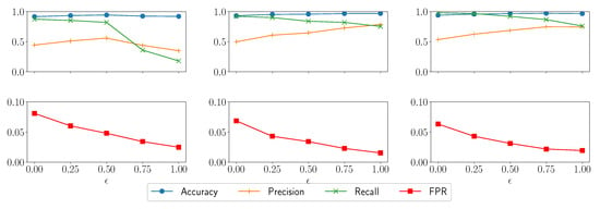
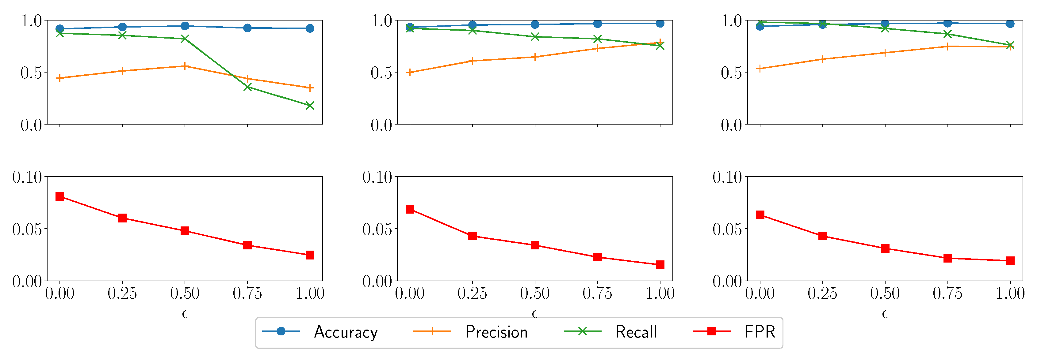
Figure 13 shows how the reporting selectivity affected the performance of the scheme in the sense of accuracy, precision, recall, and FPR in the UsA-5 scenario when the anomaly intensity $\gamma$ was 1.0, 2.0, and 3.0, respectively. In all of the three cases, when $ϵ$ increased from 0 to 1.0, the FPR decreased significantly. The recall also decreased, while the accuracy remained at a high level with a slightly upward trend. The precision increased monotonically in the cases of $\gamma$ = 2.0 and 3.0, because the reduction of false positives was faster than the reduction of true positives. In the case of $\gamma$ = 1.0, the precision decreased when $ϵ$ approached 1.0, since the reduction of true positives overtook the reduction of false positives.

Figure 13. Effect of reporting selectivity on detection performance (from left to right: $\gamma =1.0,2.0,3.0$).

The ROC-based threshold computation algorithm seeks the trade-off between TPR and FPR, without giving TPR (i.e., recall) extra weights. If recall has a higher priority than FPR in an anomaly detection task, we should preferentially adopt PADSV or PADSV-DT with a small $ϵ$ value.

3.4. Effect of Verification Probability

Requiring prompt and accurate verification from the field engineers for every alarm may be a strong assumption that is difficult to realize, especially when a pollution event is quite subtle. The field engineers may not be able to determine whether pollution did occur, or the verification process may take a longer time than the measurement interval. What if the anomaly detection process executing the PADSV scheme does not always receive the verification? In the experiments, we varied the probability of getting verification and collected the performance data for various probabilities.

In the case with incomplete verification, PADSV discarded the measurements that were detected as anomalous but were not verified, and replaced them with predicted values when making future predictions. This is different from ${\mathcal{S}}_0$, in which measurements that were detected as anomalous were kept in the history; only missing values were filled with the predicted values. PADSV with verification probability 1.0 behaved exactly the same as the original design described in Section 2.

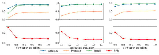
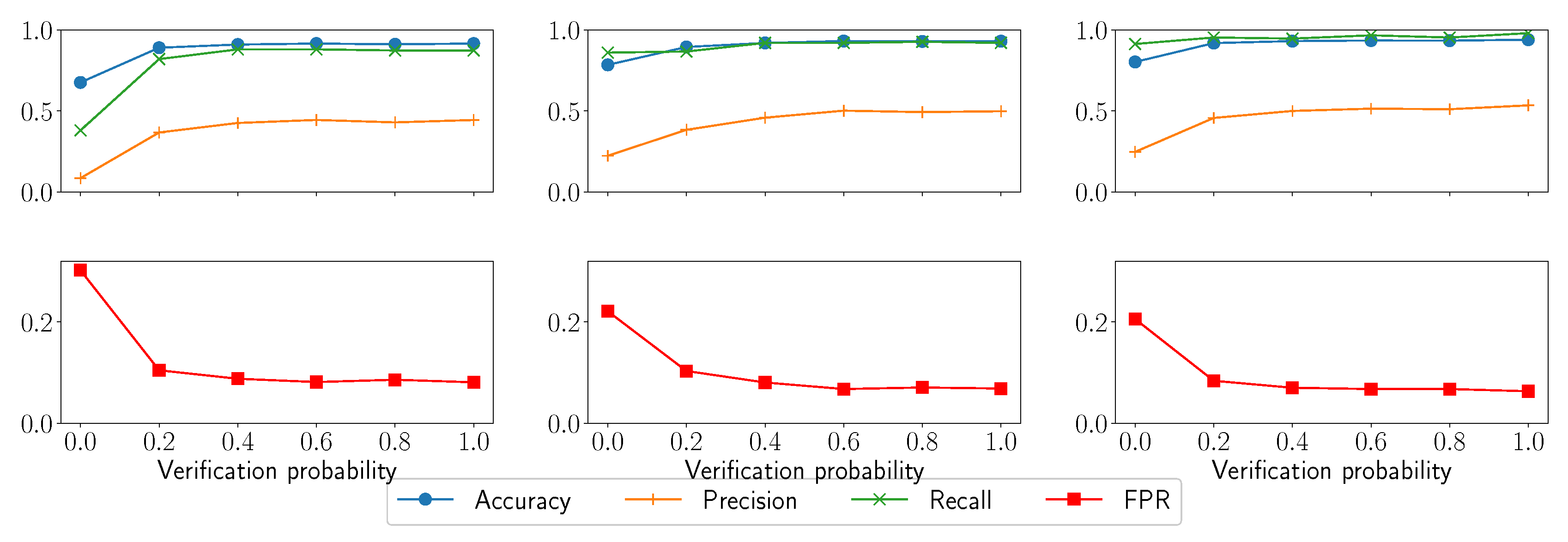
Figure 14 shows the results of PADSV in the UsA-5 scenarios with $\gamma =1.0,2.0$ and $3.0$. From the figure, we are delighted to see that verification for even a small fraction of detected anomalies had a significant impact on the performance. Without verification, the scheme suffered low recall and high FPR; with 20% verification, it boasted greatly improved recall, FPR, and overall accuracy, especially in the case of low anomaly intensity ($\gamma =1.0$). The detection performance changed little when the verification probability increased from 0.2 to 1.0. Therefore, when PADSV is deployed in the real world, we do not demand verification for every alarm, which is a relief for field engineers.

Figure 14. Effect of verification probability on detection performance (from left to right: $\gamma =1.0,2.0,3.0$).

3.5. Time Performance

We measured the detection time of PADSV and PADSV-DT on the self-collected datasets. For the sequences consisting of five water quality parameters, the average detection time of PADSV for each instance was 103 ± 5 ms (95% confidence level) on the CPU. When dynamic thresholding was enabled, the detection was slightly slower (110 ± 4 ms). Thus, the scheme can meet the real-time requirement. However, if data from hundreds of monitoring stations need to be processed simultaneously, then multiple computers should be deployed to share the load, so that anomalies at each station can be detected promptly.

The offline training procedure is performed at regular time intervals, and does not have strict time constraints. As for the self-collected datasets, the training time was about 1.6 s per epoch per water quality parameter on the CPU. Thus, for five water quality parameters and 50 epochs (the training and validation losses usually converged before this number of epochs), the training took approximately 400 s. Since data from different monitoring stations often exhibit different variation patterns, separate models should be trained for each station. If one computer system manages multiple stations, the training procedure should be scheduled to balance the use of the computing resource.

3.6. Performance on the Public Dataset

Table 5 shows the performance data of the five schemes on the GECCO2018 dataset. As one of the state-of-the-art anomaly detection algorithms, USAD achieved an impressive recall rate of 0.9073 at the cost of triggering false alarms for 9.22% of the actual negative instances. The prediction-based and verification-free scheme, ${\mathcal{S}}_0$, achieved precision and recall rates both a little lower than USAD, with a comparable FPR. However, by utilizing selective verification, PADSV significantly boosted the recall rate to 0.9907, meaning that it captured almost all of the anomalies in the test sequence, with a slightly higher FPR. The performance of PADSV was very close to that of ${\mathcal{S}}_1$, a theoretical scheme with every instance verified. By dynamically adjusting the anomaly score threshold, PADSV-DT reduced the false alarms down to 10% of those of PADSV, at the cost of a lower recall rate (0.9635; still higher than that of USAD). As a result, its precision was boosted significantly.

Table 5. Performance on the GECCO2018 dataset.

Scheme	Accuracy	Precision	Recall	FPR
USAD	0.9078	0.1577	0.9073	0.0922
${\mathcal{S}}_0$	0.9013	0.1097	0.8523	0.0980
${\mathcal{S}}_1$	0.9005	0.1225	0.9936	0.1008
PADSV	0.8997	0.1214	0.9907	0.1016
PADSV-DT	0.9891	0.5653	0.9635	0.0105

The performance gain of PADSV and PADSV-DT over USAD can be attributed to the two components in the design. First, by using a prediction-based approach and inspecting the prediction residuals, the schemes are more sensitive to the fluctuations in the time sequence, compared with USAD, which inspects the actual measurements directly. Second, by utilizing verification results from field engineers, even though partially, the schemes are able to keep their prediction on the normal track, without being distorted by anomalous instances.

4. Discussion

As we have seen from the experimental results, PADSV significantly improves the detection performance by utilizing the verification results from field engineers, compared with the schemes that do not employ verification. This is especially true for U-shaped anomalies which are often caused by pollution events and are more complicated than single-point anomalies.

For a pollution event, finding the pollution source and recovering the water quality may take a long time (or maybe nothing can be done until the pollution naturally fades out). A scheme without using verification may adapt to the anomalous data and fail to raise alarms, even before the pollution has been cleared. However, PADSV would keep sending alarms until the water quality goes back to normal, which is more acceptable in real-world water quality monitoring.

Would the detection performance improve if a non-verification-based scheme autonomously replaced the measurements that had been detected anomalous with the predicted values? The answer is negative based on our experiments and analysis. Such a feature may help boost the True Positive Rate at the beginning. However, prediction errors and short-term water quality fluctuations may cause occasional false positives at normal times. If actual measurements were replaced with the predicted values at these time points, the prediction errors would be augmented as the snowball effect and more false positives and false negatives would occur in the future. This again shows the power of verification, which helps keep the prediction on the track of normal water quality variation.

While prompt verification and feedback does put a burden on the field engineers, PADSV only requests verification for instances that have positive detection results, which amount to a small fraction of total instances. We observed that in various experiments where 10% of measurements were actual anomalies, the percentage of reported instances by PADSV, in the form of alarms, was always only slightly more than 10%. Compared with the ${\mathcal{S}}_1$ scheme, which requires verification for every instance, PADSV achieves similar performance with greatly reduced verification cost. Moreover, even if the alarms are not all verified, PADSV can still maintain high detection performance. Our experiments showed that the degradation in performance was negligible when only 20% of alarms were verified. What is the lower bound of the verification rate in order to maintain reasonable performance, given a certain rate of anomalies in a time sequence? Answers to this question would help us establish the minimal requirement of the field engineers’ effort. The question remains unsolved in this study, which we will investigate in future research.

On the other hand, when no verification is received for an alarm, PADSV does replace the detected anomalous data with predicted values. So the risk of prediction error propagation still exists, especially when the field engineers fail to verify multiple alarms in a row. Due to time limitations, the problem was not analyzed in this study, which may be another topic of our future work.

It seems that dynamic thresholding is not an indispensable feature in water quality anomaly detection, since coverage (i.e., capturing as many anomalies as possible) has usually a higher priority than labor cost in such applications and the Isolation Forest algorithm already has great detection capability. However, it may be useful in other application areas where reducing the false alarm rate has a higher priority than coverage.

Water resources in the natural environment are highly affected by human activities and meteorological factors; accordingly, the collected water quality time sequences often show nonlinear and non-stationary characteristics, with a mixture of long-term fluctuations and short-term abrupt changes. While it is of great significance to explore the impact of normal human activities on the nearby water resources in the long run, such an impact can only be mitigated by governmental and economic policies and regulations. The scope of our study, however, is to detect pollution events and equipment failures that cause short-term anomalies in water quality, so that proper actions can be taken in a timely fashion to reduce the loss and to recover the health of the water resources. If the water quality changes slowly over a long period, similar to the test scenarios with very low anomaly intensities, our scheme may not be able to detect such changes and may instead learn the trend as the new normal pattern. Therefore, the proposed scheme is not proper for the detection of long-term gradual deterioration of water quality.

Due to the non-stationary characteristics of water quality, anomaly detection models should be regularly updated with new data, in order to accurately detect anomalies which do not fit the new pattern. We believe that the ideas of human verification and historical data management in PADSV can also be applied to other existing approaches to achieve durative water quality monitoring and anomaly detection.

While PADSV was derived from our work on water quality time sequences, it is also applicable to anomaly detection in other fields.

References

- Jiang, X.; Zhang, H.; Wang, X.; Zhang, X.; Ding, K. Comprehensive analysis of the association between human diseases and water pollutants. Int. J. Environ. Res. Public Health 2022, 19, 16475. [Google Scholar] [CrossRef] [Scilit] [PubMed]
- Morin-Crini, N.; Lichtfouse, E.; Liu, G.; Balaram, V.; Ribeiro, A.R.L.; Lu, Z.; Stock, F.; Carmona, E.; Teixeira, M.R.; Picos-Corrales, L.A.; et al. Worldwide cases of water pollution by emerging contaminants: A review. Environ. Chem. Lett. 2022, 20, 2311–2338. [Google Scholar] [CrossRef] [Scilit]
- Mendivil-Garcia, K.; Amabilis-Sosa, L.E.; Guadalupe Salinas-Juarez, M.; Pat-Espadas, A.; Rodriguez-Mata, A.E.; Figueroa-Perez, M.G.; Roe-Sosa, A. Climate change impact assessment on a tropical river resilience using the Streeter-Phelps dissolved oxygen model. Front. Environ. Sci. 2022, 10, 903046. [Google Scholar] [CrossRef] [Scilit]
- Lung, W.S. Progression of river BOD/DO modeling for water quality management. Water Environ. Res. 2023, 95, e10864. [Google Scholar] [CrossRef] [Scilit]
- Peterson, K.T.; Sagan, V.; Sloan, J.J. Deep learning-based water quality estimation and anomaly detection using Landsat-8/Sentinel-2 virtual constellation and cloud computing. GISci. Remote Sens. 2020, 57, 510–525. [Google Scholar] [CrossRef] [Scilit]
- Rigueira, X.; Olivieri, D.; Araujo, M.; Saavedra, A.; Pazo, M. Multivariate functional data analysis and machine learning methods for anomaly detection in water quality sensor data. Environ. Model. Softw. 2025, 190, 106443. [Google Scholar] [CrossRef] [Scilit]
- Bi, J.; Yuan, M.; Yuan, H.; Wang, Z.; Qiao, J. Water quality anomaly detection with dual sliding windows and convolutional LSTM. In Proceedings of the IEEE International Conference on Systems, Man, and Cybernetics (SMC), Kuching, Malaysia, 6–10 October 2024; pp. 3559–3564. [Google Scholar] [CrossRef] [Scilit]
- Liu, J.; Wu, D.; Mohammed, H.; Seidu, R. A novel method for anomaly detection and signal calibration in water quality monitoring of an urban water supply system. Water 2024, 16, 1238. [Google Scholar] [CrossRef] [Scilit]
- Bourelly, C.; Bria, A.; Ferrigno, L.; Gerevini, L.; Marrocco, C.; Molinara, M.; Cerro, G.; Cicalini, M.; Ria, A. A preliminary solution for anomaly detection in water quality monitoring. In Proceedings of the IEEE International Conference on Smart Computing (SMARTCOMP), Bologna, Italy, 14–17 September 2020; pp. 410–415. [Google Scholar] [CrossRef] [Scilit]
- Almuhtaram, H.; Zamyadi, A.; Hofmann, R. Machine learning for anomaly detection in cyanobacterial fluorescence signals. Water Res. 2021, 197, 117073. [Google Scholar] [CrossRef] [Scilit]
- Obiri, N.; Maina, C.; Kiragu, H. Anomaly detection for raw water quality—A comparative analysis of the local outlier factor algorithm and the random forest algorithms. Int. J. Comput. Appl. 2021, 174, 47–54. [Google Scholar] [CrossRef] [Scilit]
- Santos-Fernandez, E.; Hoef, J.M.V.; Peterson, E.E.; McGree, J.; Villa, C.A.; Leigh, C.; Turner, R.; Roberts, C.; Mengersen, K. Unsupervised anomaly detection in spatio-temporal stream network sensor data. Water Resour. Res. 2024, 60, e2023WR035707. [Google Scholar] [CrossRef] [Scilit]
- Audibert, J.; Michiardi, P.; Guyard, F. USAD: UnSupervised Anomaly Detection on multivariate time series. In Proceedings of the 26th ACM International Conference on Knowledge Discovery and Data Mining (KDD), Virtual Event, USA, 23–27 August 2020. [Google Scholar] [CrossRef] [Scilit]
- Jiang, J.; Zheng, Y.; Pang, T.; Wang, B.; Chachan, R.; Tian, Y. A comprehensive study on spectral analysis and anomaly detection of river water quality dynamics with high time resolution measurements. J. Hydrol. 2020, 589, 125175. [Google Scholar] [CrossRef] [Scilit]
- Ni, Q.; Cao, X.; Zhao, Z.; Yuan, J.; Tan, C. An unsupervised water quality anomaly detection method based on a combination of time-frequency analysis and clustering. Environ. Sci. Pollut. Res. 2024, 31, 15920–15931. [Google Scholar] [CrossRef] [Scilit]
- Zhang, Y.; Wang, F.; Zhao, W.; Xu, F.; Zhang, J.; Jiang, S. Water quality anomaly detection: An improved empirical wavelet transform method. Water Resour. 2025, 52, 581–598. [Google Scholar] [CrossRef] [Scilit]
- Li, W.; Zhao, Y.; Zhu, Y.; Dong, Z.; Wang, F.; Huang, F. Research progress in water quality prediction based on deep learning technology: A review. Environ. Sci. Pollut. Res. 2024, 31, 26415–26431. [Google Scholar] [CrossRef] [Scilit]
- Zhang, Q.; You, X.Y. Recent advances in surface water quality prediction using artificial intelligence models. Water Resour. Manag. 2024, 38, 235–250. [Google Scholar] [CrossRef] [Scilit]
- Yan, X.; Zhang, T.; Du, W.; Meng, Q.; Xu, X.; Zhao, X. A comprehensive review of machine learning for water quality prediction over the past five years. J. Mar. Sci. Eng. 2024, 12, 159. [Google Scholar] [CrossRef] [Scilit]
- Li, T.; Comer, M.L.; Delp, E.J.; Desai, S.R.; Mathieson, J.L.; Foster, R.H.; Chan, M.W. Anomaly scoring for prediction-based anomaly detection in time series. In Proceedings of the IEEE Aerospace Conference, Big Sky, MT, USA, 7–14 March 2020; pp. 1–7. [Google Scholar] [CrossRef] [Scilit]
- Liu, J.; Wang, P.; Jiang, D.; Nan, J.; Zhu, W. An integrated data-driven framework for surface water quality anomaly detection and early warning. J. Clean. Prod. 2020, 251, 119145. [Google Scholar] [CrossRef] [Scilit]
- Wang, L.; Dong, H.; Cao, Y.; Hou, D.; Zhang, G. Real-time water quality detection based on fluctuation feature analysis with the LSTM model. J. Hydroinform. 2023, 25, 140–149. [Google Scholar] [CrossRef] [Scilit]
- Liao, Z.; Zhang, M.; Chen, Y.; Zhang, Z.; Wang, H. A “prediction-detection-judgment” framework for sudden water contamination event detection with online monitoring. J. Environ. Manag. 2024, 355, 120496. [Google Scholar] [CrossRef] [Scilit]
- Jiang, D.; Zhu, H.; Liu, J.; Feng, X.; Ma, F.; Wang, J. Dynamic surface river pollution identification by a hybrid multivariate-based anomaly detection algorithm. J. Clean. Prod. 2024, 467, 142923. [Google Scholar] [CrossRef] [Scilit]
- McAfee, B.J.; Pradhan, A.; Neog, A.; Fatemi, S.; Hensley, R.T.; Lofton, M.E.; Karpatne, A.; Carey, C.C.; Hanson, P.C. LakeBeD-US: A benchmark dataset for lake water quality time series and vertical profiles. Earth Syst. Sci. Data 2025, 17, 3141–3165. [Google Scholar] [CrossRef] [Scilit]
- Karim, M.R.; Syeed, M.M.M.; Rahman, A.; Rabbani, K.A.; Fatema, K.; Khan, R.H.; Hossain, M.S.; Uddin, M.F. A comprehensive dataset of surface water quality spanning 1940–2023 for empirical and ML adopted research. Sci. Data 2025, 12, 391. [Google Scholar] [CrossRef] [Scilit] [PubMed]
- Dogo, E.M.; Nwulu, N.I.; Twala, B.; Aigbavboa, C.O. Empirical comparison of approaches for mitigating effects of class imbalances in water quality anomaly detection. IEEE Access 2020, 8, 218015–218036. [Google Scholar] [CrossRef] [Scilit]
- Chen, X.; Liu, H.; Xu, X.; Zhang, L.; Lin, T.; Zuo, M.; Huang, Y.; Shen, R.; Chen, D.; Deng, Y. Identification of suitable technologies for drinking water quality prediction: A comparative study of traditional, ensemble, cost-sensitive, outlier detection learning models and sampling algorithms. ACS ES&T Water 2021, 1, 1676–1685. [Google Scholar] [CrossRef] [Scilit]
- Luo, W.; Huang, L. Prediction-based real-time anomaly detection for water quality time sequences. In Proceedings of the 4th International Conference on Computational Modeling, Simulation and Data Analysis (CMSDA), Hangzhou, China, 6–8 December 2024; pp. 364–371. [Google Scholar] [CrossRef] [Scilit]
- Luo, W.; Huang, L.; Shu, J.; Feng, H.; Guo, W.; Xia, K.; Fang, K.; Wang, W. Predicting water quality in municipal water management systems using a hybrid deep learning model. Eng. Appl. Artif. Intell. 2024, 133, 108420. [Google Scholar] [CrossRef] [Scilit]
- Bahdanau, D.; Cho, K.; Bengio, Y. Neural machine translation by jointly learning to align and translate. In Proceedings of the 3rd International Conference on Learning Representations (ICLR), San Diego, CA, USA, 7–9 May 2015. [Google Scholar]
- Liu, F.T.; Ting, K.M.; Zhou, Z.H. Isolation forest. In Proceedings of the 8th IEEE International Conference on Data Mining (ICDM), Pisa, Italy, 15–19 December 2008; pp. 413–422. [Google Scholar] [CrossRef] [Scilit]
- Rodriguez-Perez, J.; Leigh, C.; Liquet, B.; Kermorvant, C.; Peterson, E.; Sous, D.; Mengersen, K. Detecting technical anomalies in high-frequency water-quality data using artificial neural networks. Environ. Sci. Technol. 2020, 54, 13719–13730. [Google Scholar] [CrossRef] [Scilit]
- Jesus, G.; Casimiro, A.; Oliveira, A. Using machine learning for dependable outlier detection in environmental monitoring systems. ACM Trans. Cyber-Phys. Syst. 2021, 5, 1–30. [Google Scholar] [CrossRef] [Scilit]
- Han, J.; Kamber, M.; Pei, J. Data Mining: Concepts and Techniques, 3rd ed.; Morgan Kaufmann Publishers: Waltham, MA, USA, 2012; pp. 113–114. [Google Scholar]
- Leigh, C.; Alsibai, O.; Hyndman, R.J.; Kandanaarachchi, S.; King, O.C.; McGree, J.M.; Neelamraju, C.; Strauss, J.; Talagala, P.D.; Turner, R.D.; et al. A framework for automated anomaly detection in high frequency water-quality data from in situ sensors. Sci. Total Environ. 2019, 664, 885–898. [Google Scholar] [CrossRef] [Scilit]
- Balta, D.; Kac, S.B.; Balta, M.; Eken, S. Water quality estimation and anomaly detection: A review. EAI Endorsed Trans. Internet Things 2023, 9, 1–20. [Google Scholar] [CrossRef] [Scilit]
- Yang, Y.J.; Haught, R.C.; Goodrich, J.A. Real-time contaminant detection and classification in a drinking water pipe using conventional water quality sensors: Techniques and experimental results. J. Environ. Manag. 2009, 90, 2494–2506. [Google Scholar] [CrossRef] [Scilit]
- Moritz, S.; Rehbach, F.; Chandrasekaran, S.; Rebolledo, M.; Bartz-Beielstein, T. GECCO industrial challenge 2018 dataset: A water quality dataset for the “Internet of Things: Online anomaly detection for drinking water quality” competition. In Proceedings of the Genetic and Evolutionary Computation Conference (GECCO), Kyoto, Japan, 15–19 July 2018. [Google Scholar] [CrossRef]
- Dogo, E.M.; Nwulu, N.I.; Twala, B.; Aigbavboa, C.O. Accessing imbalance learning using dynamic selection approach in water quality anomaly detection. Symmetry 2021, 13, 818. [Google Scholar] [CrossRef] [Scilit]
- Wang, X.; Li, Y.; Qiao, Q.; Tavares, A.; Liang, Y. Water quality prediction based on machine learning and comprehensive weighting methods. Entropy 2023, 25, 1186. [Google Scholar] [CrossRef] [Scilit]
Disclaimer/Publisher’s Note: The statements, opinions and data contained in all publications are solely those of the individual author(s) and contributor(s) and not of MDPI and/or the editor(s). MDPI and/or the editor(s) disclaim responsibility for any injury to people or property resulting from any ideas, methods, instructions or products referred to in the content. |
© 2026 by the authors. Licensee MDPI, Basel, Switzerland. This article is an open access article distributed under the terms and conditions of the Creative Commons Attribution (CC BY) license.