Coordinated Control of Valves and Protective Devices for Pressure Drop Mitigation in Gravity Irrigation Systems

Abstract

To address pressure-drop-induced safety risks in high-drop gravity-fed irrigation pipelines, this study investigates coordinated prevention and control strategies that integrate air release and vacuum valve groups with flow-adaptive valve closure rules. A large-scale self-pressurized irrigation network (1.33 × 10⁸ m²) in Karamay, Xinjiang, China, is selected as a representative case study. Based on one-dimensional transient flow modeling, pressure drop and negative-pressure characteristics induced by inlet valve closure in the main pipeline are analyzed using wave speed theory, governing differential equations, and the finite difference method. A coordinated protection framework is proposed that explicitly links valve operating patterns with the spatial configuration of protective devices. Unlike conventional schemes that rely on empirical layouts and fixed closure rules, this study introduces a critical-flow-velocity-based valve grouping method combined with flow-dependent valve closure strategies. Simulation results demonstrate that a strategically optimized configuration of air release and vacuum valves along the main pipeline is sufficient to eliminate negative pressure under all operating conditions. For flow rates below 6 m³/s, linear valve closure ensures safe operation, whereas a two-stage closure is required for higher flow rates (6–10 m³/s). As flow increases, reducing the fast-closure ratio and extending the total closure time effectively suppress pressure-drop-dominated transient effects at vulnerable inlet sections. By effectively mitigating transient pressure surges, the proposed coordinated “valve closure-protection device” strategy improves system adaptability to flow variability and provides practical engineering guidance for the safe operation of gravity irrigation systems, particularly high-gradient self-pressurized networks.

1. Introduction

Gravity irrigation systems rely on terrain elevation differences to achieve gravity-driven water flow without additional power. They play a crucial role in agricultural irrigation in arid and semi-arid regions with uneven water distribution. Across Central Asia, irrigated lands contribute the dominant share of regional crop production (≈80%), underscoring the representative and transferable value of gravity-fed schemes in arid oases; in Xinjiang, China, recent policies and practice emphasize large-scale expansion of water-saving irrigation (e.g., extensive drip irrigation targets), making the Karamay self-pressurized network a typical case with broader relevance [1,2,3]. These systems are key to improving water use efficiency and ensuring stable agricultural production [4]. Such systems typically consist of long-distance water conveyance pipelines, valves, pump stations, and other core components. Their safe operation directly impacts the lifespan and effectiveness of irrigation projects. However, during actual operation, valve closures, sudden pump shutdowns, and similar actions can easily trigger pressure transients, including pressure rise and pressure drop. These phenomena may cause severe issues such as pipeline rupture, joint loosening, cavitation, and column separation [5,6]. Especially in high-gradient gravity flow pipelines, the concentrated hydraulic potential energy intensifies pressure-transient-induced fluctuations, resulting in more severe damage risks [7].

Water hammer is a general term describing transient pressure waves in pressurized pipelines; often called the silent killer in water conveyance systems, it is essentially a pressure transient caused by sudden changes in fluid momentum. In long-distance water transport projects, these transient pressures can reach several times the steady-state value—at minimum causing pipeline vibrations and [8], in severe cases, leading to pipe bursts [9,10]. Classical water hammer theory indicates that sudden changes in flow velocity caused by valve closures or pump station failures trigger pressure waves. The intensity of these pressure fluctuations is directly related to the water hammer wave speed, which is influenced by both the fluid’s compressibility and the pipe material’s elastic modulus [11]. Existing studies have extensively investigated the mitigation and control of water hammer-related pressure transients, using numerical simulations and experimental approaches to optimize protective-device layouts and valve operation strategies. For example, air release and vacuum valves effectively mitigate negative pressure through gas–liquid exchange. However, their spacing and configuration must be dynamically adjusted based on the pipeline topology and critical flow velocity [11,12,13]. The two-stage valve closure strategy significantly reduces pressure peaks by controlling the rate of flow velocity change, demonstrating superior performance compared to linear valve closure [14,15]. Further research shows that using variable-rate valve closure can delay the occurrence of pressure peaks, thereby enhancing safety beyond that achieved with traditional piecewise-linear valve closures [16]. Building on these strategy-level advances, mechanistic studies of valve–transient interactions provide crucial underpinning and limits: Bergant, Simpson, and Tijsseling synthesized the column-separation/rejoining mechanism and its coupling with closure maneuvers, identifying triggers of extreme over-/under-pressure and local cavitation dynamics [17]; however, their analysis is largely single-device/single-scenario, with limited coverage of time-segmented, periodic operations typical of irrigation networks. Subsequently, Meniconi et al. experimentally demonstrated the self-adjusting dynamics of pressure-relief valves (PRVs), showing how inherent valve response reshapes local waveforms and peak timing [18]; yet these studies were conducted under simplified boundaries and single-valve settings, without closed-loop multi-valve/networked coordination. On the modeling side, Vítkovský et al. systematically evaluated one-dimensional unsteady-friction formulations—convolution/weight function versus instantaneous acceleration—thereby clarifying their impact on peak prediction and damping [19]; still, quasi-steady inflows are typically assumed, and closure timing/rate laws are not co-designed. Extending this, Duan et al. quantified scale effects (pipe length/diameter) on the relevance of unsteady friction [20]; yet the linkage to seasonal flow variability and coordinated device placement remains open. Moreover, Tijsseling highlighted fluid–structure interaction (FSI) in long or thick-walled pipes, warning that neglecting wall elasticity/structural vibration biases wave propagation and peaks [21]; this line of work, however, focuses on FSI physics rather than co-optimizing operations and protections under periodic regulation. In sum, despite progress at both strategy and mechanism levels, most studies still assume steady or idealized inflows and single-device contexts, leaving a gap in closed-loop coordinated optimization that links flow-adaptive closure timing/rates with the spatial configuration of protective devices under periodic irrigation scheduling. To operationalize the above closed-loop coordinated optimization, a quantitative “mechanism–operation interface” is needed; here, 3-D CFD provides several viable routes for resolving near-valve flows and transient pressures during maneuvers, including dynamic meshes, sliding meshes, immersed-solid/immersed-boundary and overset-mesh approaches, each with distinct accuracy–cost trade-offs [22]. Comparative studies indicate that, for selected cases, sliding meshes reproduce peak pressures and wall shear with high fidelity, whereas dynamic-mesh and immersed-solid formulations can achieve acceptable accuracy at comparable or lower cost [22]; general 3-D frameworks have been applied to pressurized-pipe transients [23] and to valve-induced water hammer with experimental comparisons and detailed flow visualization [24]; and overset meshes offer a robust option for complex valve kinematics [25]. Building on these advances, we treat 3-D CFD as a complement to operational design: by resolving near-valve vortex-core evolution and peak timing to calibrate the rates and trigger thresholds of two-stage or variable-rate closures, while simultaneously diagnosing under-pressure/cavitation-prone regions to inform the spatial optimization of air/vacuum-valve placement, and—when coupled with 1-D MOC—enabling a closed-loop co-design of operations and protections [26].

In long-distance water conveyance projects, the coordinated optimization of protective devices and valve operations is crucial for enhancing system safety. Especially under extreme conditions such as pipe bursts, employing a combined “fast closure + slow closure” strategy for upstream and downstream valves can simultaneously reduce leakage and suppress secondary pressure-transients effects [9]. Previous studies have shown that combining air chambers with PRVs can achieve the same level of surge protection with fewer or smaller devices, while keeping maximum pressure fluctuations within safe limits [10,27]. Moreover, coordinated regulation of multiple valves can further mitigate pressure surges through the interference effects of water hammer waves [28,29,30]. In gravity flow systems, the high-pressure water hammer at the pipeline outlet and negative-pressure risks at the inlet are particularly pronounced. Therefore, differentiated valve closure strategies are necessary: prolonged or two-stage valve closure is recommended at the outlet, while enhanced air release and vacuum capabilities are required at the inlet [31,32,33]. Typical cases show that applying a 400 s two-stage valve closure at the inlet (75% fast closure + 25% slow closure) can completely eliminate negative pressure. At the outlet, a 600 s two-stage closure (85% fast closure + 15% slow closure) reduces the maximum positive pressure by over 40% compared to linear closure, while shortening the closure time to one-fifth [34]. However, existing coordinated optimization schemes face two major limitations in agricultural irrigation contexts: first, the layout of protective devices relies heavily on empirical formulas and lacks closed-loop feedback with valve operations; second, valve closure strategies are not adapted to the seasonal flow fluctuations of irrigation networks. This results in insufficient research on water hammer-coordinated prevention and control for self-pressurized irrigation pipelines, especially in high-gradient, large-flow agricultural irrigation scenarios [35,36,37]. Such systems often face challenges including significant terrain variations, wide flow fluctuations, and complex branch networks. Traditional protection schemes suffer from poor adaptability and low economic efficiency in addressing these issues [38,39].

Therefore, the primary objective of this study is to propose a coordinated optimization strategy integrating flow-adaptive valve operational control and critical-velocity-based protective device configuration to mitigate water hammer risks in high-gradient gravity irrigation systems.

2. Materials and Methods

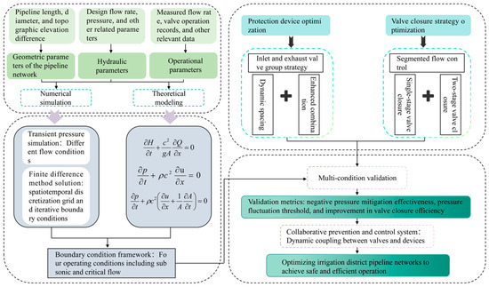
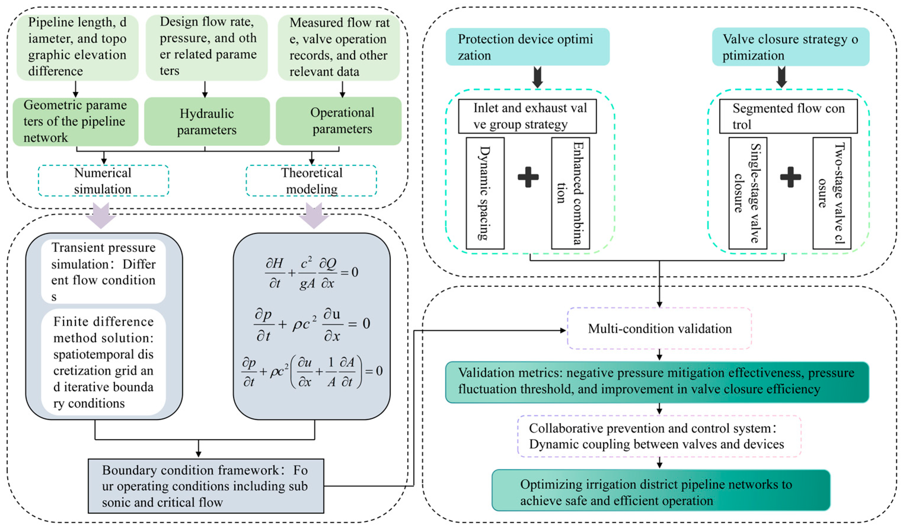
To address the complex transient pressure challenges in high-gradient gravity irrigation systems, this study focuses on a 1.33 × 10⁸ m² self-pressurized network in Karamay, Xinjiang, China. Unlike conventional water hammer protection studies that design valve operation strategies and protection-device layouts independently, this research adopts a multi-method integrated approach to examine their combined effects within a unified analytical framework that reflects actual operating characteristics. First, based on pipeline fluid mechanics, differential governing equations for water hammer are established to quantify pressure wave propagation. Subsequently, numerical simulation techniques utilizing the finite difference method are applied to discretize and solve these equations in time and space, accurately capturing transient pressure field distributions under complex boundary conditions. Within this numerical framework, the spatial deployment of air release and vacuum valves is optimized through a grouping approach based on critical flow velocity and gas–liquid exchange dynamics, ensuring the protection configuration responds dynamically to local hydraulic sensitivities. Concurrently, a flow-adaptive, segmented two-stage valve-closing strategy is formulated through comparative verification across multiple scenarios, adjusting the closing timing and angle ratios based on operational flow rates rather than relying on a single prescribed condition. Together, these theoretical and numerical methods support the construction of a dynamic, coordinated prevention and control system integrating valve operation and protective devices. The complete technical approach and logical framework are illustrated in Figure 1.

Figure 1. Methodological framework.

2.1. Water Hammer Effect Calculation and Analysis Methods

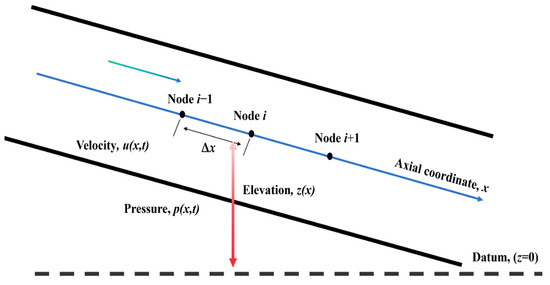
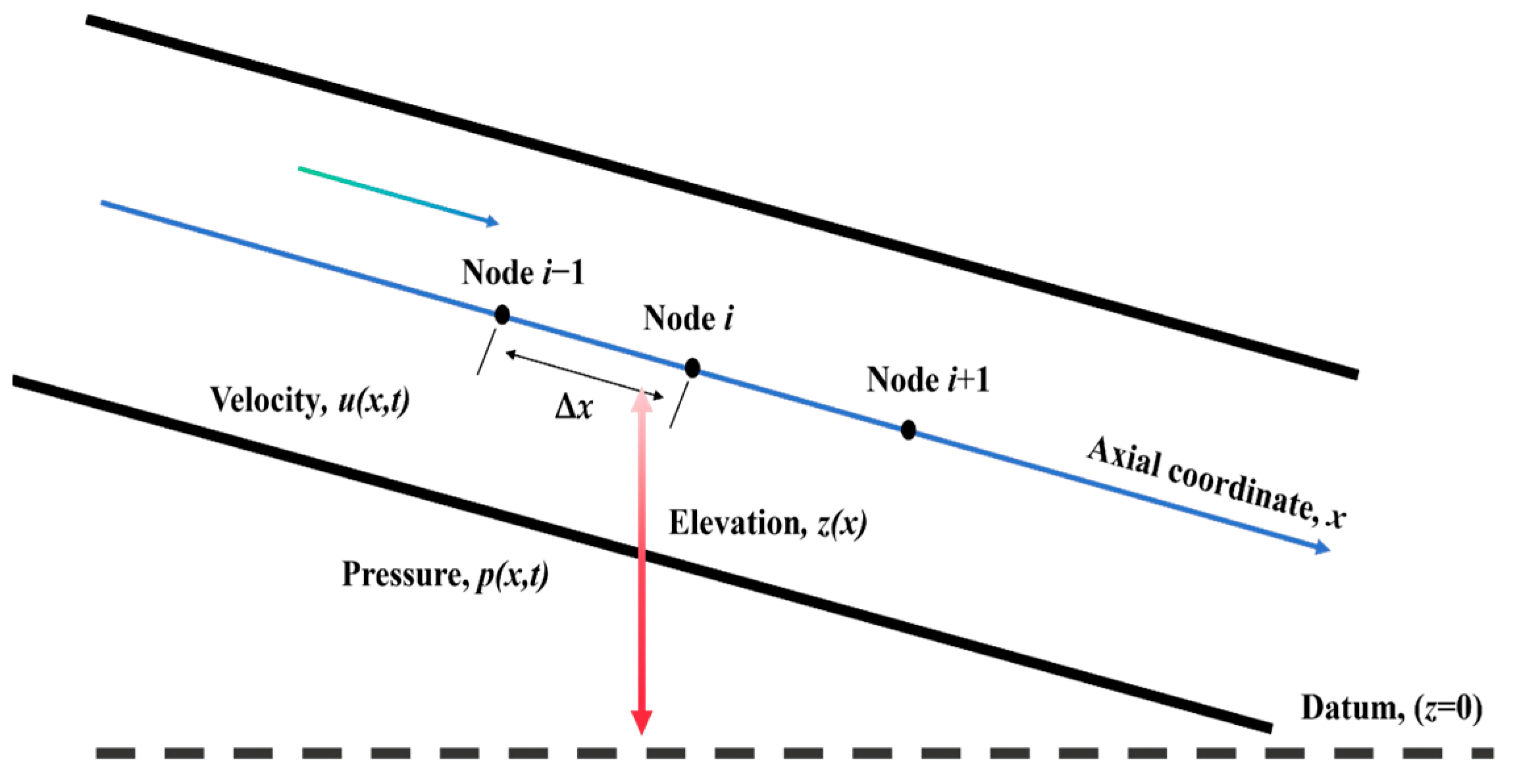
Water hammer risk during pipeline valve closure arises from rapid changes in fluid momentum that generate pressure waves. In this study we formulate a pressurized, full-bore transient model based on one-dimensional, cross-sectionally averaged conservation laws and standard water hammer theory, and we solve the resulting equations numerically to quantify pressure and velocity transients under different valve closure schedules. To clearly illustrate the one-dimensional hydraulic system under consideration and the spatial discretization of the mathematical model, a schematic diagram of the pipeline within the established coordinate system is presented in Figure 2. As shown, the longitudinal axis x aligns with the pipeline centerline, while z(x) represents the elevation head relative to a horizontal datum. The transient flow variables, including cross-sectional mean velocity u(x,t) and pressure p(x,t), are defined along this axis. For the subsequent finite difference solution, the spatial domain is discretized into continuous nodes (e.g., i − 1, i, i + 1) separated by a spatial step of Δx.

Figure 2. Schematic diagram of the one-dimensional pipeline transient flow model.

(1)

Calculation of water hammer wave velocity. For a thin-walled elastic pipe, the effective wave speed c is given by the Korteweg expression [40]:

$$c={\displaystyle \frac{\sqrt{\frac{K}{\rho }}}{\sqrt{1+\frac{KD}{Ee}}}}$$

(1)

where K is the fluid bulk modulus, ρ density, E Young’s modulus of the wall, e the wall thickness, and D the internal diameter of the pipe. In this study, the effective wave speed is taken as c = 1000 m/s for the steel main pipeline, which is a practical value for water in rigid metallic pipes.

(2)

Governing momentum equation. With the axial coordinate x along the pipeline and the terrain elevation z(x), the 1-D cross-sectionally averaged momentum equation reads as follows [40,41]:

$${\displaystyle \frac{\partial \mathrm{u}}{\partial \mathrm{t}}}+{\displaystyle \frac{1}{\rho }}{\displaystyle \frac{\partial p}{\partial x}}+\mathrm{g}{\displaystyle \frac{\partial z}{\partial \mathrm{x}}}+{\displaystyle \frac{f}{2D}}u\left|u\right|+{\displaystyle \frac{{\displaystyle \sum K_m}}{2\Delta x}}u\left|u\right|=0$$

(2)

where u(x,t) is the mean axial velocity, p(x,t) pressure, ρ density, g gravity, D pipe diameter, and f the Darcy–Weisbach friction factor, and z(x) denotes the pipeline elevation profile along the axial coordinate x. Additionally, to accurately capture the impact of local flow resistance, a generic minor loss term has been explicitly incorporated into the momentum equation, where K_m represents the minor loss coefficient for valves or structural fittings, and Δx is the local spatial discretization step over which the loss is distributed.

(3)

Transient continuity equation (pressurized full-bore). Since the pipe is fully filled and the geometric cross-section A is constant in time, the unsteady mass conservation is [40,41]

$${\displaystyle \frac{\partial p}{\partial t}}+\rho c^2{\displaystyle \frac{\partial u}{\partial x}}=0$$

(3)

where the wave speed c accounts for fluid compressibility and wall elasticity. The more general form

$${\displaystyle \frac{\partial p}{\partial t}}+\rho c^2\left({\displaystyle \frac{\partial u}{\partial x}}+{\displaystyle \frac{1}{A}}{\displaystyle \frac{\partial A}{\partial t}}\right)=0$$

(4)

reduces to the equation above when the pipe cross-sectional area (A) is treated as a constant and the pipe wall elasticity is incorporated into the wave speed (c). Because this study assumes the pipeline remains fully pressurized with a constant cross-sectional area during transient events, the term ${\displaystyle \frac{1}{A}}{\displaystyle \frac{\partial A}{\partial t}}$ vanishes, allowing Equation (4) to effectively reduce to Equation (3).

Introducing discharge Q = Au and piezometric head H = p/(ρg) + z, Equations (2) and (3) are equivalently written as [40]

$${\displaystyle \frac{\partial H}{\partial t}}+{\displaystyle \frac{c^2}{gA}}{\displaystyle \frac{\partial Q}{\partial x}}=0$$

(5)

$${\displaystyle \frac{\partial Q}{\partial t}}+gA{\displaystyle \frac{\partial H}{\partial x}}+{\displaystyle \frac{f}{2DA}}\left|Q\right|Q=0$$

(6)

which naturally embeds gravity via the elevation z(x).

The finite difference method is used to solve the basic differential equations and transient continuity equations. The pipeline space is discretized into equally spaced grids. To ensure physical consistency, a lower bound corresponding to absolute vacuum was imposed on the computed gauge pressure head. Pressures below −10 m were not interpreted as further physical pressure reduction, but as indicators of cavitation or air admission through vacuum valves, and were truncated at this limit for post-processing and visualization.

With spatial and temporal steps Δx and Δt, a first-order explicit scheme for Equations (2) and (3) is

$$p_i^{n+1}=p_i^n-\rho c^2{\displaystyle \frac{\Delta t}{\Delta x}}\left(u_i^n-u_{i-1}^n\right)$$

(7)

$${\mathrm{u}}_i^{n+1}=u_i^n-{\displaystyle \frac{\Delta t}{\rho \Delta x}}\left(p_{i+1}^n-p_i^n\right)-g\Delta t\left({\displaystyle \frac{z_{i+1}-z_i}{\Delta x}}\right)-{\displaystyle \frac{f\Delta t}{2D}}{u}_i^n\left|u_i^n\right|$$

(8)

The Courant condition cΔt/Δx ≤ 1 is enforced for stability. Unsteady (frequency-dependent) friction, if required, can be incorporated via the Zielke/Vardy–Brown weighting-function approach [42].

2.2. Design and Validation Methods of Safety Protection Measures

To address the high vulnerability of the main pipeline, an air release and intake valve group is used for water hammer protection. The specific methods are as follows:

2.2.1. Air Release and Intake Valve Arrangement Scheme

(1)

Spacing design is based on empirical design values combined with dynamic adjustment of the critical flow velocity V_c. Here, V_c is defined as the cross-sectionally averaged flow velocity at which sub-atmospheric pressure first appears at the inlet section during valve closure transients in the baseline simulation without additional air valve grouping. When the cross-sectionally averaged flow velocity u exceeds V_c, the spacing between air valves is increased; otherwise, it is reduced.

(2)

Valve group optimization: Multiple valve groups are installed at bends near the pipeline inlet. Their combined operation is simulated to eliminate negative pressure.

(3)

Standards-based deployment: In terms of valve selection, arrangement, and operation strategies, this study follows internationally recognized standards for the operation and protection of gravity pipeline systems. Specifically, it refers to AWWA M51 (Air-Release, Air/Vacuum, and Combination Air Valves) [43] for principles related to valve selection, spacing design, and installation locations. This standard recommends installing combination air valves at pipeline high points, elevation breaks, long horizontal sections, and locations prone to air accumulation, in order to effectively prevent negative pressure and air entrapment. Based on this standard, the design of the main pipeline in this study prioritizes the placement of valves at these critical locations.

2.2.2. Boundary Condition Verification

Based on nozzle gas dynamics principles, boundary condition equations are established for four operating scenarios to ensure efficient gas–liquid exchange. The formulas are as follows:

(1)

Air flows in as subsonic isentropic flow [44]. (p₀ > p > 0.5283 p₀)

$$\stackrel{•}{m}=C_{in}{A}_{in}\sqrt{7p_0{\rho }_0\left[{\left({\displaystyle \frac{p}{p_0}}\right)}^{1.4286}-{\left({\displaystyle \frac{p}{p_0}}\right)}^{1.714}\right]}$$

(9)

where m represents the air mass flow rate through the air valve cross-section; C_in is the flow coefficient when air enters the valve; A_in is the inlet area of the air valve (m²); p is the absolute gas pressure inside the air valve (MPa); and p₀ is the atmospheric pressure (MPa).

(2)

Air flows in as isentropic flow at critical velocity [44]. (p ≤ 0.5283 p₀)

$$\stackrel{•}{m}=C_{in}{A}_{in}{\displaystyle \frac{0.686}{\sqrt{R{T}_0}}}{p}_0$$

(10)

where R is the gas constant, and T₀ is the atmospheric temperature in Kelvin (K).

(3)

Air flows out as subsonic isentropic flow [44].

$$\stackrel{•}{m}=-C_{out}{A}_{out}p\sqrt{{\displaystyle \frac{7}{RT}}\left[{\left({\displaystyle \frac{p_0}{p}}\right)}^{1.4286}-{\left({\displaystyle \frac{p_0}{p}}\right)}^{1.7143}\right]}$$

(11)

where C_out is the flow coefficient for air exiting the air valve; A_out is the outlet area of the air valve (m²); and T is the gas temperature inside the air valve (K).

(4)

Air flows out as isentropic flow at critical velocity [44].

$$\stackrel{•}{m}=-C_{out}{A}_{out}{\displaystyle \frac{0.686}{\sqrt{R{T}_0}}}p$$

(12)

2.2.3. Effectiveness Verification

The pressure characteristics at different flow rates of 5 m³/s and 9.5 m³/s were simulated using software after installing the valve groups to evaluate improvements in vulnerability.

For the initial condition at time t = 0, the pipeline is assumed to operate under a steady-state flow prior to any valve operation. Thus, the initial flow rate is uniform along the pipeline, given by Q(x,0) = Q₀, and the initial piezometric head distribution H(x,0) is governed by steady-state friction losses from the upstream source. Based on the modeling framework described above, boundary conditions were defined to represent typical operating conditions of the self-pressurized gravity irrigation system. The upstream boundary at x = 0 was treated as a constant-head reservoir. Reflecting the relatively large storage capacity of the water source compared with transient flow variations, short-term water-level fluctuations were neglected, yielding the upstream boundary condition H(0,t) = H_res. All transient events analyzed in this study were initiated by the inlet butterfly valve. The downstream boundary at x = L was represented by a prescribed time-dependent valve-controlled condition corresponding to practical irrigation operations; the downstream valve operated under controlled conditions and did not serve as an independent trigger of transients. No additional surge protection devices were considered at the downstream end. Along the pipeline, the flow was assumed to remain fully pressurized, with air–water mass exchange occurring only through the air release and vacuum valves considered above.

2.3. Valve-Closing Model Development

Two valve closure models are proposed: linear closure and two-stage closure. In the linear closure of a slow-closing butterfly valve, the closing angle decreases linearly over time. In the two-stage closure process, the fast-closing phase lasts for t₁ with a fast-closing angle of φ₁, while the slow-closing phase lasts for t₂ with a slow-closing angle of φ₂. The closing angle θ at any given time t can be determined as follows:

$$\theta ={\displaystyle \frac{{\varphi }_1}{t_1}}t$$

(13)

$$\theta ={\varphi }_1+{\displaystyle \frac{{\varphi }_2}{t_2}}(t-t_1)$$

(14)

$${\varphi }_1+{\varphi }_2={90}^{\circ }$$

(15)

where θ is the closing angle (°); t is the time (h); t₁ is the fast-closing duration (h); t₂ is the slow-closing duration (h); φ₁ is the fast-closing angle (°); and φ₂ is the slow-closing angle (°).

When 0 ≤ t ≤ t₁, the valve is in the fast-closing phase and the closing angle follows Equation (13); when t₁ < t ≤ t₁ + t₂, the valve enters the slow-closing phase governed by Equation (14); when t ≥ t₁ + t₂, the valve is assumed to be fully closed, and the closing angle reaches its maximum value θ_max = φ₁ + φ₂ = 90°, as defined in Equation (15).

2.4. Model Validation and Sensitivity Analysis Setup

2.4.1. Model Validation Procedures

As detailed in Section 2.1 and Section 2.2, the model’s reliability and physical consistency are ensured through strict numerical and empirical controls. Specifically, the Courant condition is enforced to guarantee numerical stability and prevent non-physical divergence during finite difference solving. Furthermore, to accurately simulate actual pipeline physics, an absolute vacuum threshold of −10 m is implemented to physically constrain extreme negative pressures. Additionally, the selection, spatial arrangement, and operation of protective devices are validated against the internationally recognized AWWA M51 standard for gravity pipeline systems, ensuring the practical engineering validity of the simulation framework.

2.4.2. Sensitivity Analysis Design

To systematically assess the robustness and generalizability of the proposed water hammer protection strategy, comprehensive parameter sensitivity analyses are incorporated into the study design. The sensitivity of the pipeline’s transient response to critical boundary and operational parameters is rigorously evaluated. These key variables include: (i) varying initial steady-flow rates ranging from 0.01 to 10.0 m³/s; (ii) different spatial configurations of air valve groups; (iii) a wide spectrum of single-stage valve-closing durations; and (iv) varying fast-closure angle ratios for the two-stage closure strategy. The detailed quantitative outcomes and dynamic pressure envelope curves for these sensitivity scenarios are extensively presented in the subsequent results, specifically in Section 3.1, Section 3.2 and Section 3.3.

2.5. Case Study

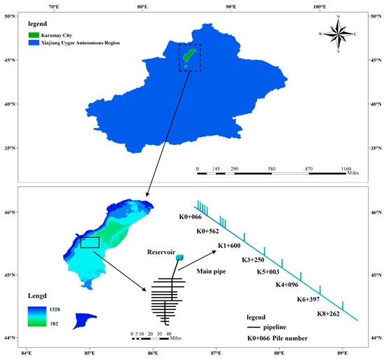
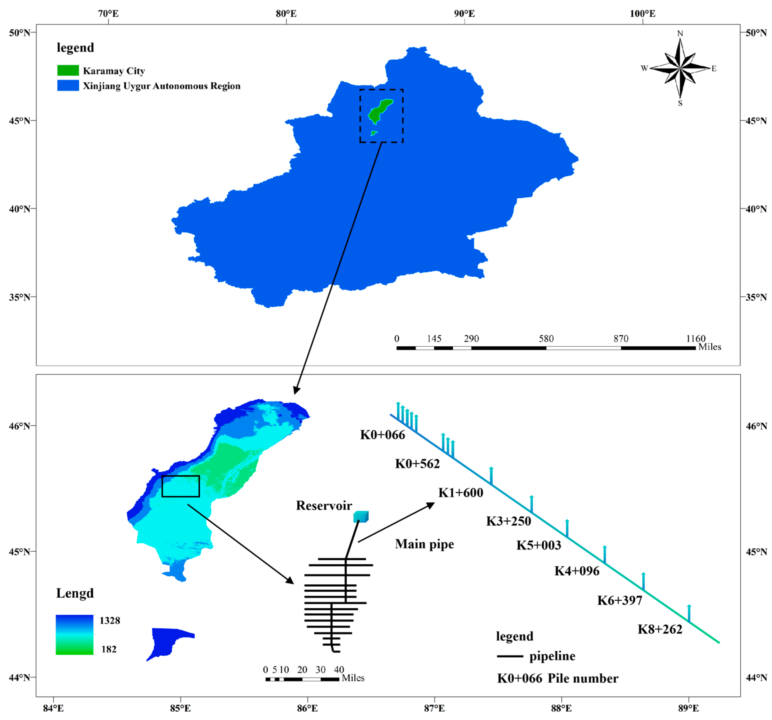
A large-scale gravity-fed irrigation system in Karamay, Xinjiang, China, is used to investigate coordinated water hammer control strategies in this paper. The irrigation network serves an agricultural area of approximately 1.33 × 10⁸ m² and is supplied by a reservoir, with water conveyed entirely under gravity-driven conditions. The modeled system consists of a steel main pipeline with a total length of 9574 m and an internal diameter of 2.20 m. The inlet elevation of the main pipeline is 351.64 m, while the terminal elevation is 273.02 m, resulting in an overall elevation drop of 78.62 m. A DN2200 butterfly valve is installed at the pipeline inlet to regulate discharge. The network further includes 28 branch pipelines with diameters ranging from DN600 to DN200, constructed from fiberglass-reinforced plastic (FRP) for diameters above 300 mm and unplasticized polyvinyl chloride (UPVC) for smaller pipes. In the numerical model, the upstream reservoir is represented by a fixed-head boundary condition, while transient flow regulation is achieved through the inlet valve. Based on this configuration, multiple operating scenarios involving different flow rates and valve-closing strategies are investigated to analyze water hammer responses and evaluate the effectiveness of coordinated protection measures. The location of the study area and the general layout of the irrigation network are shown in Figure 3.

Figure 3. Study area map (k0+066 represent the engineering chainage (pile numbers), indicating the longitudinal distance from the pipeline inlet).

3. Results

3.1. Pressure Simulation Analysis of the Main Pipeline Without Protective Measures

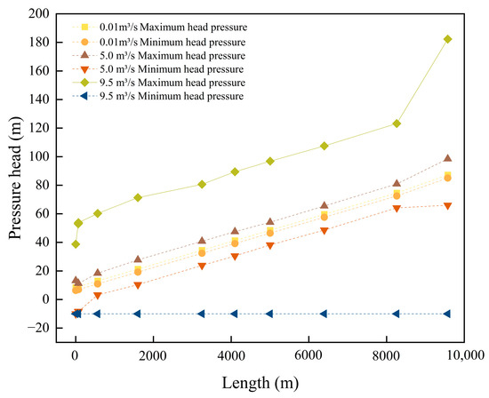
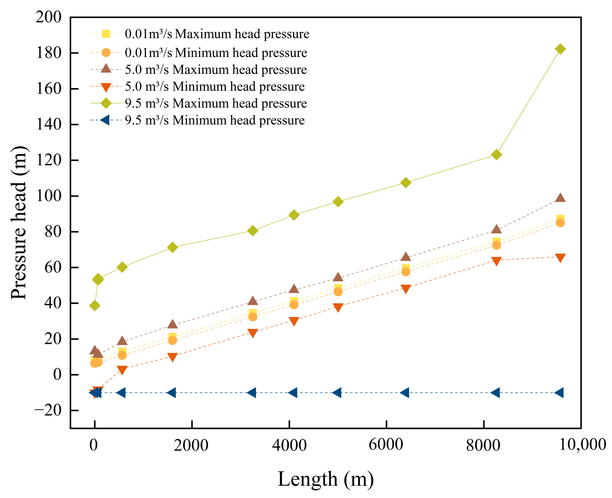
The transient (unsteady) flow and valve transient processes of the pressurized pipeline system were simulated using numerical software to model water hammer events. The main pipeline was modeled to reproduce the pipeline operating conditions and to obtain time-history curves of the pressure head for analysis of water hammer effects. Numerical simulations were performed for the main pipeline under different flow rates. Valve closure pressure transients were simulated for flow rates of 0.01, 5.0, and 9.5 m³/s. The results are presented in Figure 4.

Figure 4. Valve-closing pressure diagram without installation of protective measures.

When the flow rate is 0.01 m³/s, the pipeline remains under positive pressure throughout the entire length, with a minimum pressure of 6.41 m water column. As the flow rate increases to 5 m³/s, the minimum pressure decreases to the physical lower bound of −10 m, indicating the onset of cavitation or vacuum conditions during valve closure. When the flow rate further increases to 9.5 m³/s, the minimum pressure also reaches −10 m, suggesting that severe sub-atmospheric pressure conditions occur over a larger portion of the pipeline. These results demonstrate that increasing flow rate significantly elevates the risk and spatial extent of sub-atmospheric pressure during valve closure.

The pressure results indicate that sub-atmospheric pressure develops at the pipeline inlet. As water is conveyed from the reservoir downstream through the diversion pipeline, rapid valve closure induces a pronounced transient pressure reduction at the inlet section. Owing to the combined effects of flow inertia and elevation change at the inlet bend, this pressure drop is most significant at the local high point. When the local pressure falls below atmospheric pressure or approaches the vapor pressure of water, column separation and the release of dissolved gas may occur, leading to the formation of a low-pressure cavity within the pipeline. This mechanism explains the simulated occurrence of negative pressure at the inlet. Meanwhile, at the pipeline outlet, the inertia of the flowing water generates impact pressures during valve closure, resulting in strong pressure fluctuations. In the absence of protective measures, the combined interaction of inlet under-pressure and outlet over-pressure intensifies the water hammer response, thereby jeopardizing the safe operation of the pipeline.

3.2. Water Hammer Protection-Coordinated Optimization of Valve Regulation

To address the water hammer damage occurring in the main pipeline, this study employs air release and vacuum valves to mitigate water hammer during valve closure. Air release and vacuum valves are therefore introduced as key protective measures against inlet sub-atmospheric pressure. When air accumulates and fluid velocity changes, water hammer can occur. Air release valves reduce this phenomenon, protecting the pipeline system and equipment. Additionally, air release valves must be spaced appropriately to avoid mutual interference, ensuring sufficient distance for normal valve operation. By setting suitable boundary conditions, the system can maintain stable operation under varying conditions, guaranteeing proper valve function. A CARX-DN200 composite air release valve is selected as the water hammer protection device. Valves are installed according to the pipeline’s terrain and structure, and pipeline pressure variations are simulated accordingly.

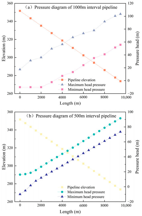
At the maximum simulated flow rate of 9.5 m³/s, the pressure variations in the pipeline after installing air release and vacuum valves were analyzed. Based on experience, these valves are typically spaced every 500–1000 m or installed at pipeline high points and bends. First, a valve spacing of 1000 m was simulated. The resulting pipeline pressure is shown in Figure 5a.

Figure 5. Pressure distribution diagram of pipelines with 500 m and 1000 m intervals.

As shown in Figure 5a, a region of negative pressure is observed within the first 3000 m of the pipeline. The negative pressure gradually intensifies along the upstream section and is eliminated at point (K3+000). At the pipeline inlet, the minimum pressure reaches −10 m water column. The simulation results indicate that installing air release valves at 1000 m intervals cannot completely eliminate the negative pressure induced by valve closure. Therefore, a second scenario was simulated with valves spaced every 500 m. The results are shown in Figure 5b.

Figure 5b shows that the length of the pipeline experiencing negative pressure is reduced from 3000 m to approximately 1000 m compared with the previous case. The minimum pressure at the pipeline inlet reaches −10 m in both cases. Although the extent of the negative-pressure region is significantly reduced, negative pressure still occurs at the pipeline inlet. This indicates that adjusting the spacing of air release valves alone cannot effectively eliminate inlet negative pressure. Therefore, it is proposed to install multiple air release valves at the negative pressure locations to form an air valve group, which can improve air release efficiency at the pipeline inlet.

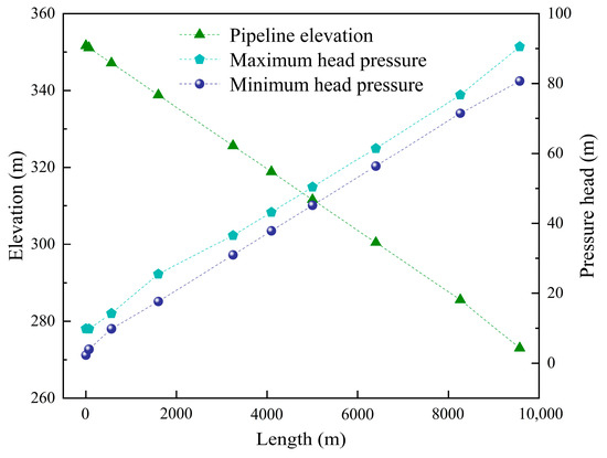
Multiple air release valves were installed at the pipeline inlet bend (K0+066) to form an air valve group, and additional groups of valves were installed at (K0+500). Combined simulations were conducted with various configurations. The results show that installing five air release valves at (K0+066) and three at (K0+500) can eliminate negative pressure at the pipeline inlet. The results are presented in Figure 6, and the pressure outcomes for each configuration are summarized in Table 1.

Figure 6. Inlet and exhaust valve combination pipe pressure diagram.

Table 1. Intake and exhaust valve combination pipeline pressure table.

Station	Number Installed	Station	Number Installed	Minimum Pipeline Pressure (m)	Maximum Pipeline Pressure (m)	Whether it Meets Requirements
K0+066	2	K0+500	1	−10.00	90.28	no
K0+066	3	K0+500	1	−9.66	88.65	no
K0+066	4	K0+500	1	−8.96	87.53	no
K0+066	5	K0+500	1	−7.74	86.69	no
K0+066	2	K0+500	2	−6.87	85.94	no
K0+066	3	K0+500	2	−5.88	84.57	no
K0+066	4	K0+500	2	−4.56	83.66	no
K0+066	5	K0+500	2	−3.49	82.95	no
K0+066	2	K0+500	3	−2.68	81.98	no
K0+066	3	K0+500	3	−1.69	81.65	no
K0+066	4	K0+500	3	−0.85	81.11	no
K0+066	5	K0+500	3	2.32	80.7	yes

According to the simulation results shown in Figure 6, installing five air release valves at (K0+066), three at (K0+500), and one valve every 1100 m along the remaining pipeline sections eliminates negative pressure throughout the entire pipeline. The minimum pressure is maintained at 2.32 m water column. The selection and placement of water hammer protection measures should ensure that sub-atmospheric pressure is avoided under all operating conditions. Adding air release valves effectively eliminates negative pressure, ensuring the pipeline operates normally and meets the required safety standards.

3.3. Optimization of Pipeline Valve Closure Time

In large-diameter, high-flow pipelines, high fluid inertia makes rapid valve closure prone to inducing excessive pressure fluctuations, necessitating staged closure strategies. High-pressure conditions in large-flow pipeline systems mean that rapid valve closure can cause local pressure spikes, potentially exceeding the pipeline’s pressure limits. Staged valve closure allows for gradual pressure release, preventing sudden pressure changes and ensuring the system pressure remains within safe limits.

3.3.1. Analysis of Single-Stage Linear Valve Closure

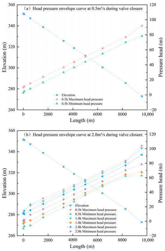
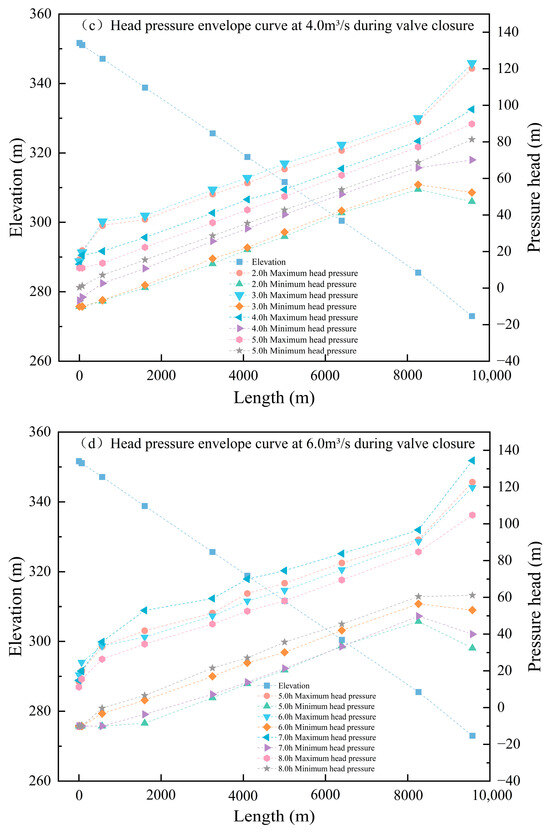
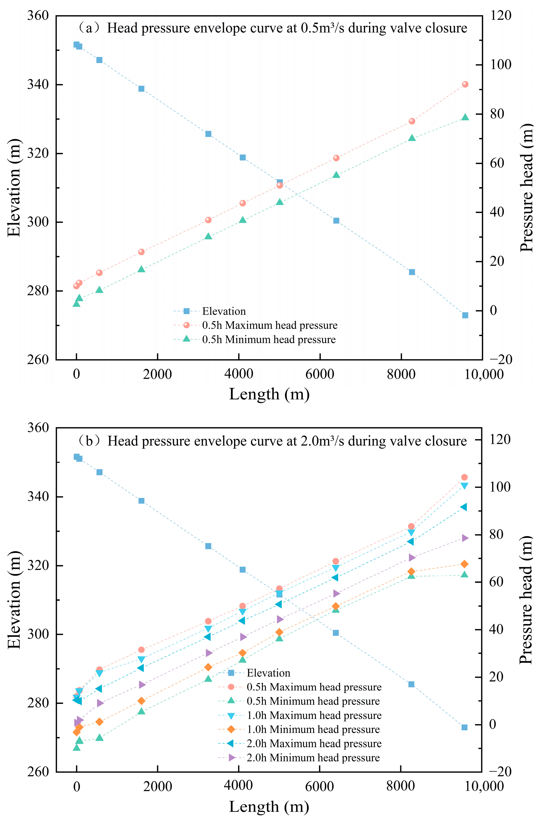
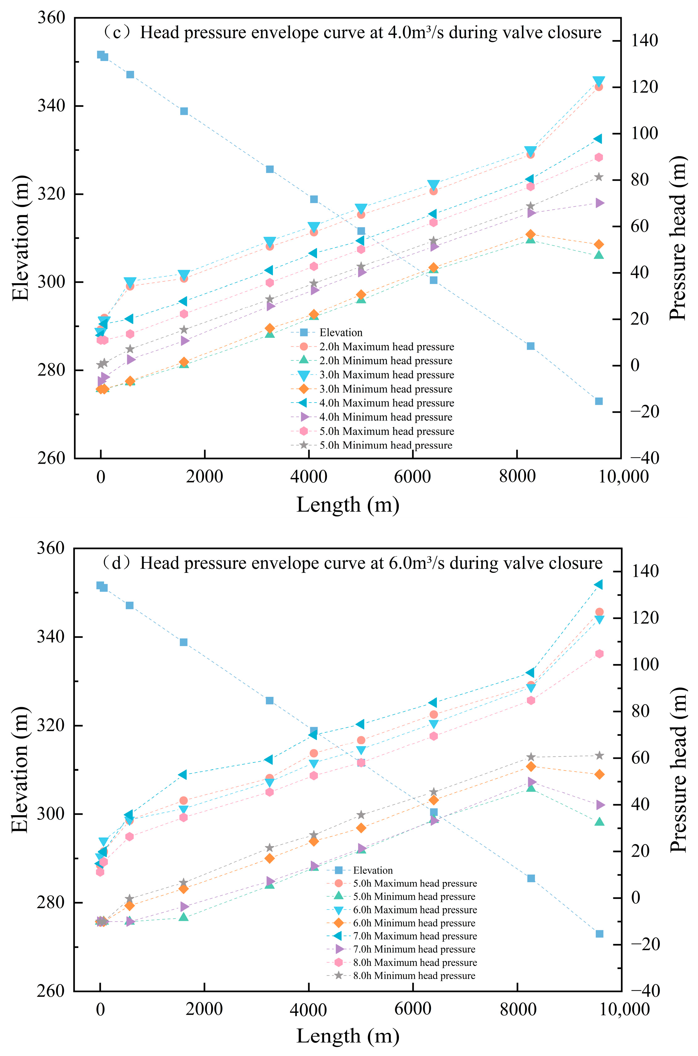
In long-distance gravity-fed water supply pipeline systems, improper valve closure or unexpected valve shutdowns due to pipeline faults can cause sudden pressure changes within the pipeline. According to crop water demand in the irrigation area, pipeline flow rates are adjusted to meet these requirements. Based on the measured operating conditions, valve closure simulations were carried out for flow rates of 0.5, 2.0, 4.0, 6.0, 8.0, and 10.0 m³/s with the valve initially fully open at 90°. Scenario 1 assumes a single-stage linear valve closure with closure durations of 0.5, 1.0, 2.0, 3.0, 4.0, and 5.0 h. The corresponding pressure results for different flow rates under this single-stage closure are shown in Figure 7.

Figure 7. One-stage closing valve pressure envelope line.

Condition 1: When the pipeline flow rate is 0.5 m³/s and a single-stage valve closure is applied over 0.5 h, the pressure variation along the pipeline is shown in Figure 7a. According to the simulation results, the pipeline remains free of negative pressure. The minimum pressure is 2.60 m water column, and the maximum pressure is 92.17 m water column. At low flow rates, single-stage valve closure can ensure safe pipeline operation during valve closure.

Condition 2: When the pipeline flow rate is 2.0 m³/s and a single-stage valve closure is applied, the simulation results are shown in Figure 7b. Valve closure times of 0.5, 1.0, and 2.0 h were simulated. At a closure time of 0.5 h, negative pressure of −10 m water column and positive pressure of 104.19 m water column occurred. At 1.0 h closure, negative pressure reduced to −3.16 m water column, with positive pressure at 100.93 m water column. As the closure time increased, both positive and negative pressures decreased. At a 2.0 h closure, no negative pressure was observed; the minimum pressure was 0.82 m water column, and the maximum pressure was 91.64 m water column, indicating safe valve closure operation.

Condition 3: When the pipeline flow rate is 4.0 m³/s and a single-stage valve closure is applied, the simulation results are shown in Figure 7c. Based on the results from Figure 7a,b, larger flow rates require longer closure times, so simulations began at 2.0 h. At a 2.0 h linear closure, the pipeline experienced negative pressure of −10 m water column. As the closure time increased to 3.0 and 4.0 h, the magnitude of negative pressure was gradually reduced, although negative pressure still occurred. Finally, at a 5.0 h closure time, no negative pressure occurred; the minimum pressure was 0.30 m water column, meeting operational safety requirements.

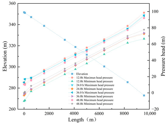
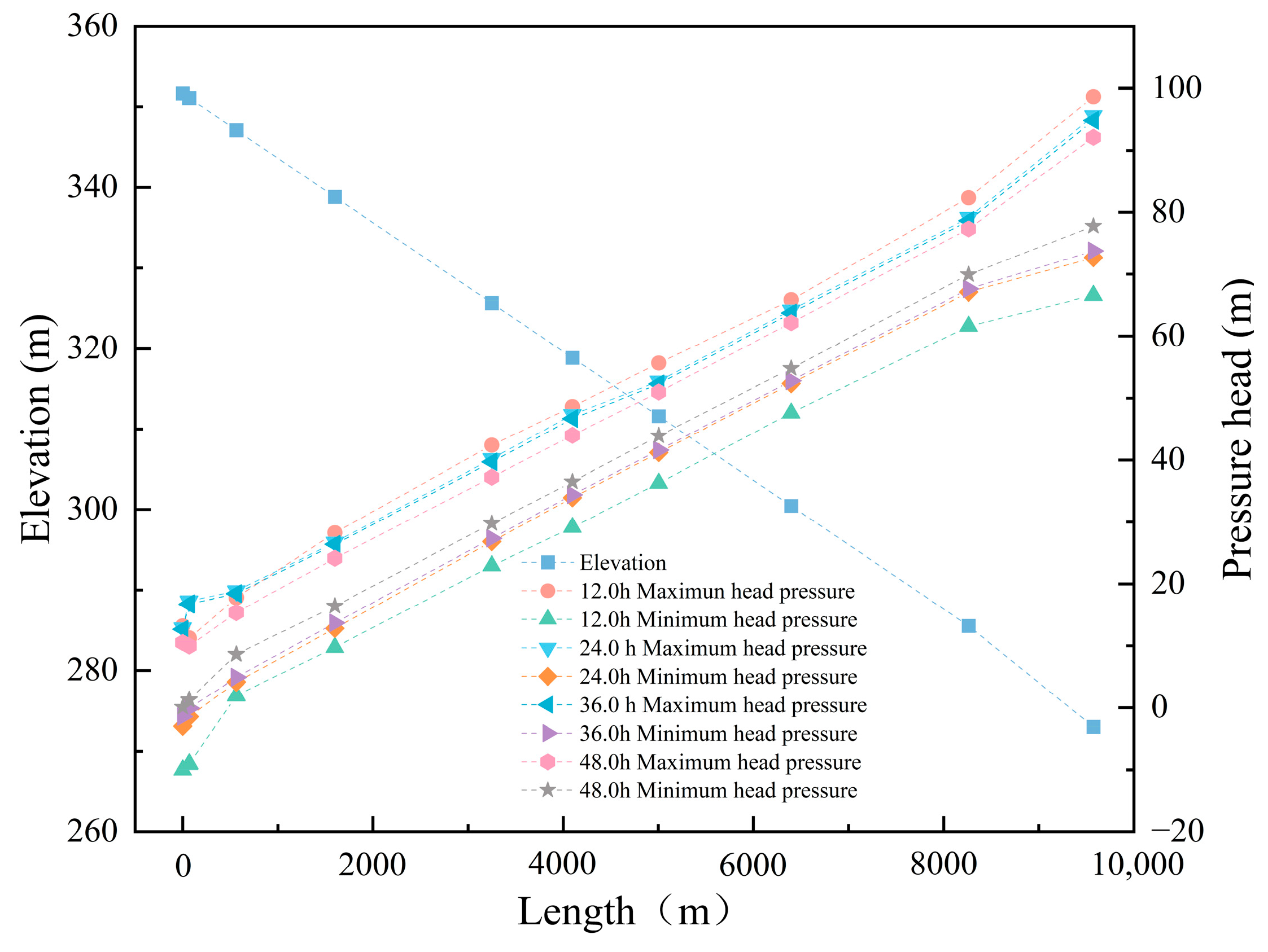
Condition 4: When the pipeline flow rate is 6.0 m³/s and a single-stage valve closure is applied, the simulation results are shown in Figure 7d. Based on previous simulations, valve closure time increases with flow rate. Closure times of 5.0, 6.0, 7.0, and 8.0 h were simulated, but negative pressure still occurred, with a minimum pressure of −10 m water column. Therefore, closure times were further extended to 12.0, 24.0, 36.0, and 48.0 h. The simulation results are presented in Figure 8.

Figure 8. 6.0 m3/s closing valve 12.0~48.0 h pipeline pressure envelope.

As the valve closure time increases, the pipeline’s negative pressure gradually decreases until it is eliminated, changing from −10 m water column at 12.0 h to 0.07 m water column at 48.0 h. Although extending closure time can safely shut the pipeline, it reduces closure efficiency. When irrigation demand decreases, excessively long valve closure times may lead to prolonged transient pressure disturbances and local pressure accumulation in branch pipelines during the regulation process, rather than under steady zero-flow conditions, which can increase structural stress and potential operational risks. Therefore, for large-diameter, high-flow pipelines, single-stage linear valve closure is inefficient. A two-stage valve closure approach can reduce closure time and improve valve closure efficiency.

3.3.2. Analysis of Two-Stage Valve Closure

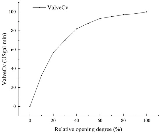
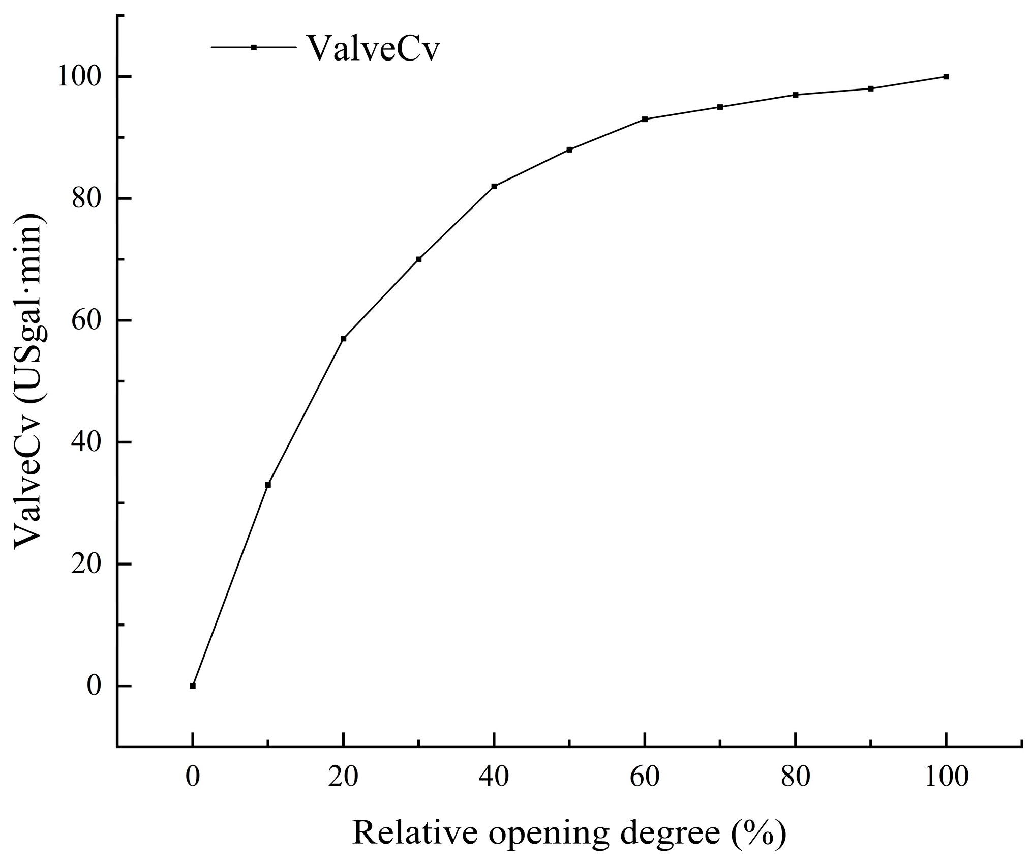
To address the issues mentioned above, Scenario 2 proposes transient calculations of valve closure time using a two-stage closure method. According to the relevant literature, the valve closure is simulated with a fast closure lasting one-third of the total time, followed by a slow closure lasting two-thirds of the time. Figure 9 shows the relationship between valve relative opening and the flow coefficient C_v. The C_v value determines the valve’s flow capacity: the higher the C_v, the greater the flow capacity and the lower the loss. When the valve opening exceeds 50%, the increase in C_v gradually slows, and the valve loss coefficient decreases accordingly.

Figure 9. Valve relative opening and Cv value relationship curve.

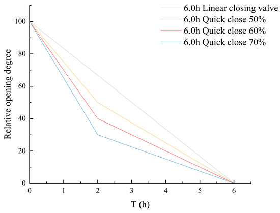
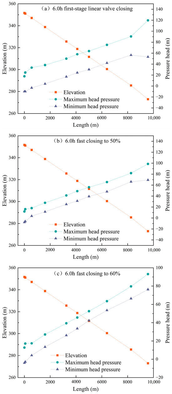
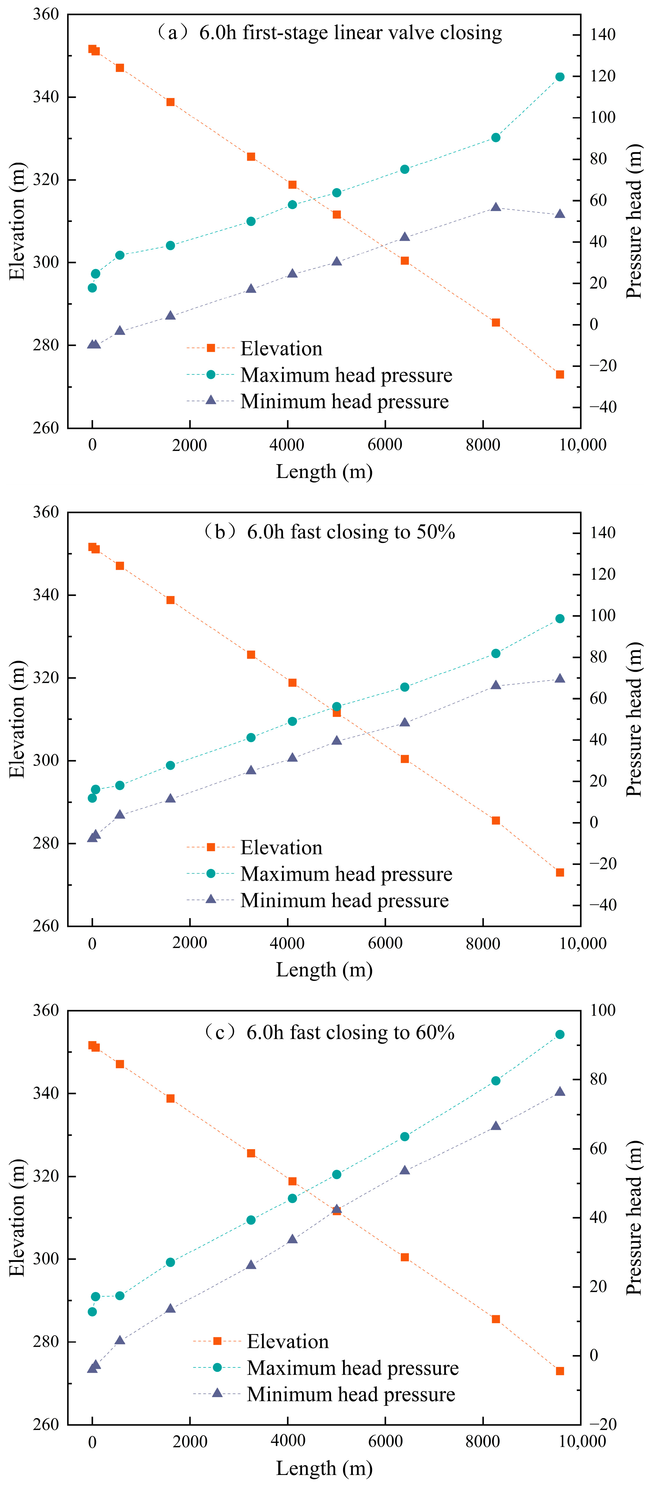
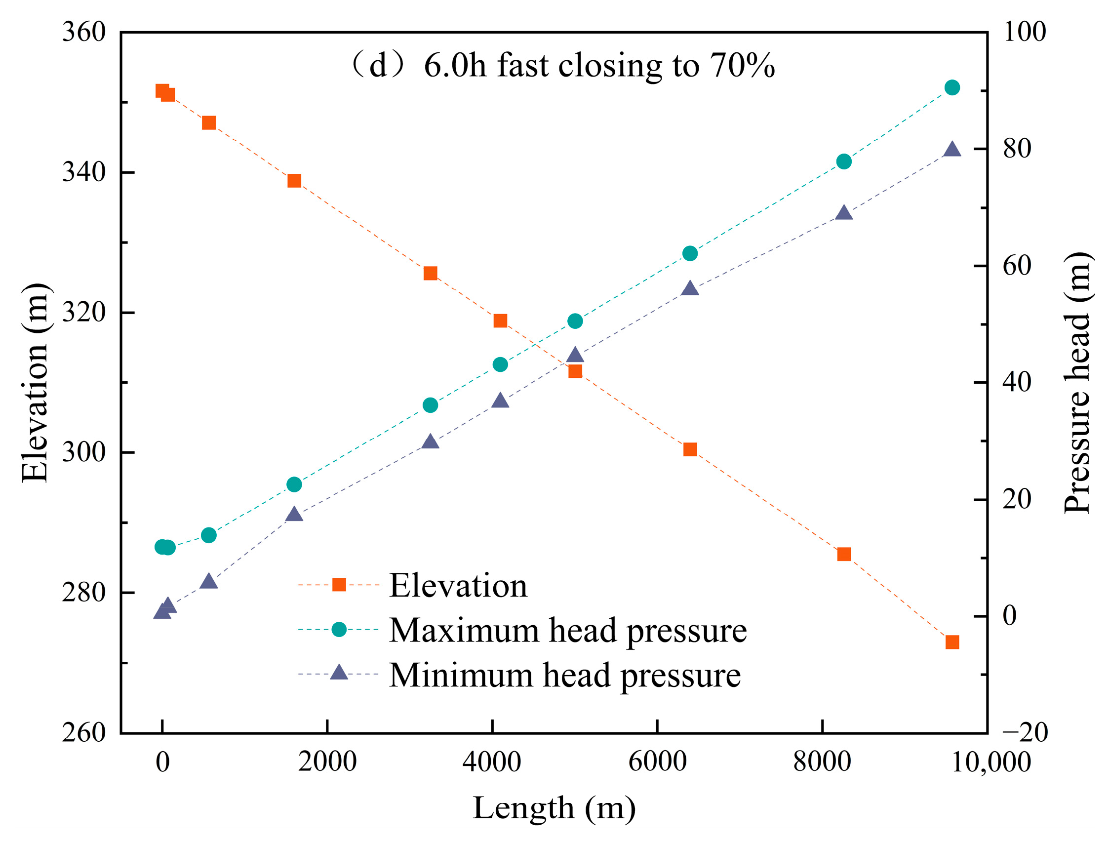
Condition 1: When the pipeline flow rate is 6.0 m³/s, a two-stage valve closure is applied with a total closure time of 6.0 h. Simulations were conducted for fast valve closures at relative openings of 50%, 60%, and 70%. The relationship between valve relative opening and closure time is shown in Figure 10, while the pressure distribution along the pipeline sections during closure is presented in Figure 11.

Figure 10. The two-stage valve-closing law of 6.0 m³/s, total valve closing time of 6.0 h.

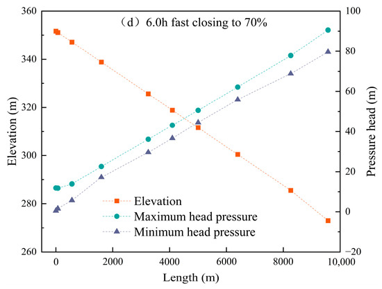
Figure 11. 6.0 m³/s total valve-closing time, 6.0 h different valve-closing angle pressure envelope.

When the pipeline flow rate is 6.0 m³/s and a two-stage valve closure is applied, the pressure at various pipeline sections is shown in Figure 11a–d. At 50% fast closure, the minimum pressure reaches −7.70 m water column. Increasing the fast-closure ratio to 60% raises the minimum pressure to −4.02 m water column. When the fast-closure ratio is further increased to 70%, the system remains entirely under positive pressure, with a minimum pressure of 0.52 m water column. Figure 11 demonstrates that two-stage valve closure effectively suppresses negative pressure. As the fast-closure opening increases from 50% to 70%, the length of the pipeline experiencing negative pressure shortens, until no negative pressure is observed at 70% fast closure. Therefore, with a total closure time of 6.0 h, applying a fast closure of 70% within the first 2.0 h followed by a slow closure of the remaining 30% eliminates negative pressure at all network nodes.

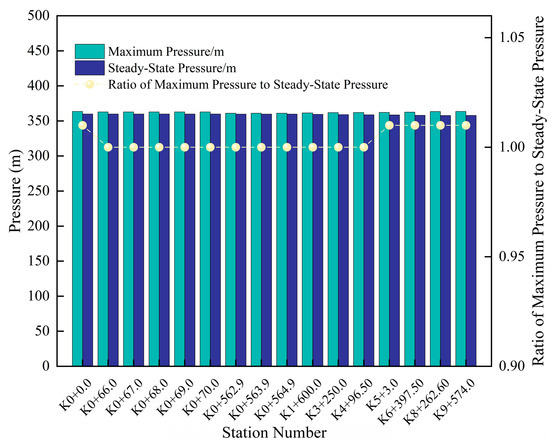
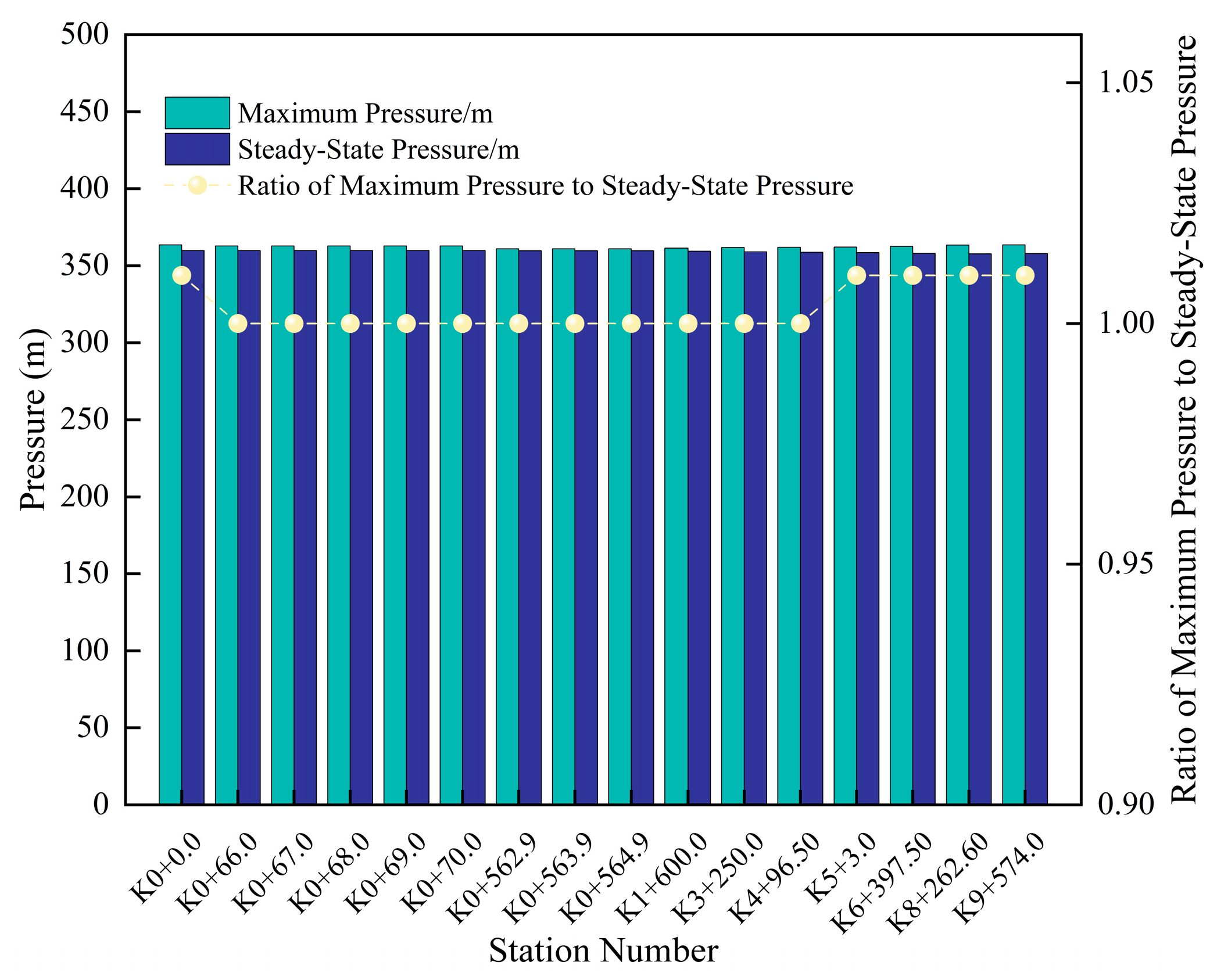
Water hammer protection measures should be designed such that the maximum transient pressure does not exceed the pipe’s nominal pressure rating (PN). The results shown in Figure 12 demonstrate that the maximum pressure throughout the pipeline remains within the allowable PN limit, confirming the pressure safety of the proposed valve-closing strategy.

Figure 12. 6.0 h two-stage 70% fast closing, and then 30% closing typical section characteristic pressure.

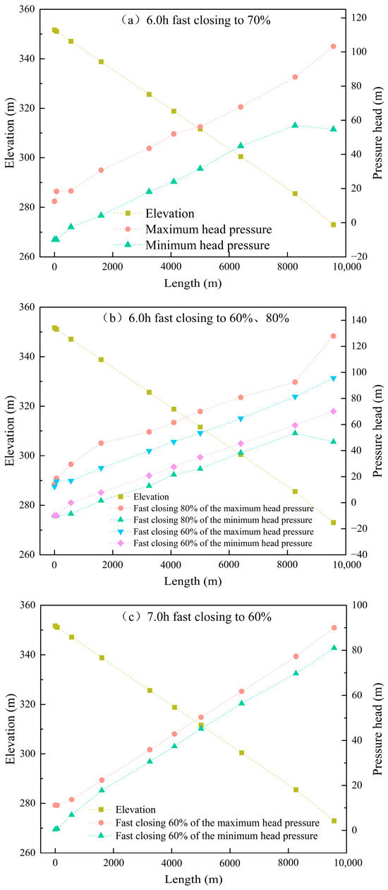
To meet peak water demand, the pipeline flow rate continues to increase. Two-stage valve closure is applied at a flow rate of 8.0 m³/s. The simulation results are shown in Figure 13.

Figure 13. 8.0 m³/s two-stage valve-closing pressure envelope.

When the pipeline flow rate is 8.0 m³/s, a two-stage valve closure with a total duration of 6.0 h was simulated. At a fast-closure ratio of 70%, negative pressure occurred, with the minimum pressure reaching −10 m, as shown in Figure 13a. The fast-closure ratio was then adjusted, and simulations were conducted for 60% and 80% fast closure, with the results shown in Figure 13b. At a total closure time of 6.0 h, reducing the fast closure ratio led to a noticeable mitigation of negative pressure; however, negative pressure still occurred. Based on the results of the two-stage valve closure simulations, it can be inferred that, under higher flow-rate conditions, reducing the fast-closure ratio and extending the total valve closure time is beneficial for alleviating negative pressure. To further examine this effect, a total closure time of 7.0 h with a fast-closure ratio of 60% was simulated. The results in Figure 13c show no negative pressure, with a minimum pressure of 0.39 m water column, meeting safety requirements. Therefore, at a flow rate of 8.0 m³/s, using a two-stage valve closure with a total closure time of 7.0 h—including 2.3 h of 60% fast closure—prevents negative pressure throughout the pipeline.

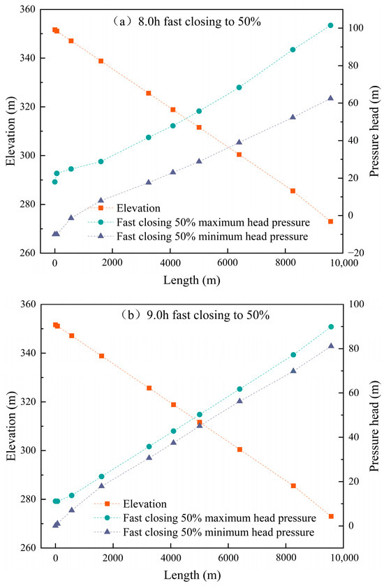
When the pipeline flow rate is 10.0 m³/s, a two-stage valve closure is applied. Based on the simulation results in Figure 13, an 8.0 h closure with 50% fast closure was simulated. The results are shown in Figure 14a.

Figure 14. 10.0 m³/s two-stage closing valve pressure envelope.

Based on the simulation results in Figure 14a, extending the valve closure time and reducing the fast-closure angle still resulted in negative pressure of −10 m water column. Due to the increased pipeline flow, the closure time was further extended to 9.0 h. However, from Figure 9, the minimum fast closure angle is 50%. The simulation results for this scenario are shown in Figure 14b. Figure 14b shows that extending the valve closure time eliminates negative pressure within the pipeline. The minimum pressure is 0.10 m water column, confirming the previous hypothesis.

When the flow rate is high, valve closure time is short, and the fast-closure angle is large, the pipeline experiences rapid flow changes and significant pressure fluctuations. This leads to intense pipeline vibrations and increases the risk of water hammer. For high-flow pipelines, using a two-stage valve closure can improve closure efficiency while mitigating water hammer effects.

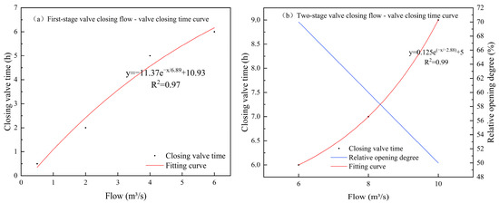
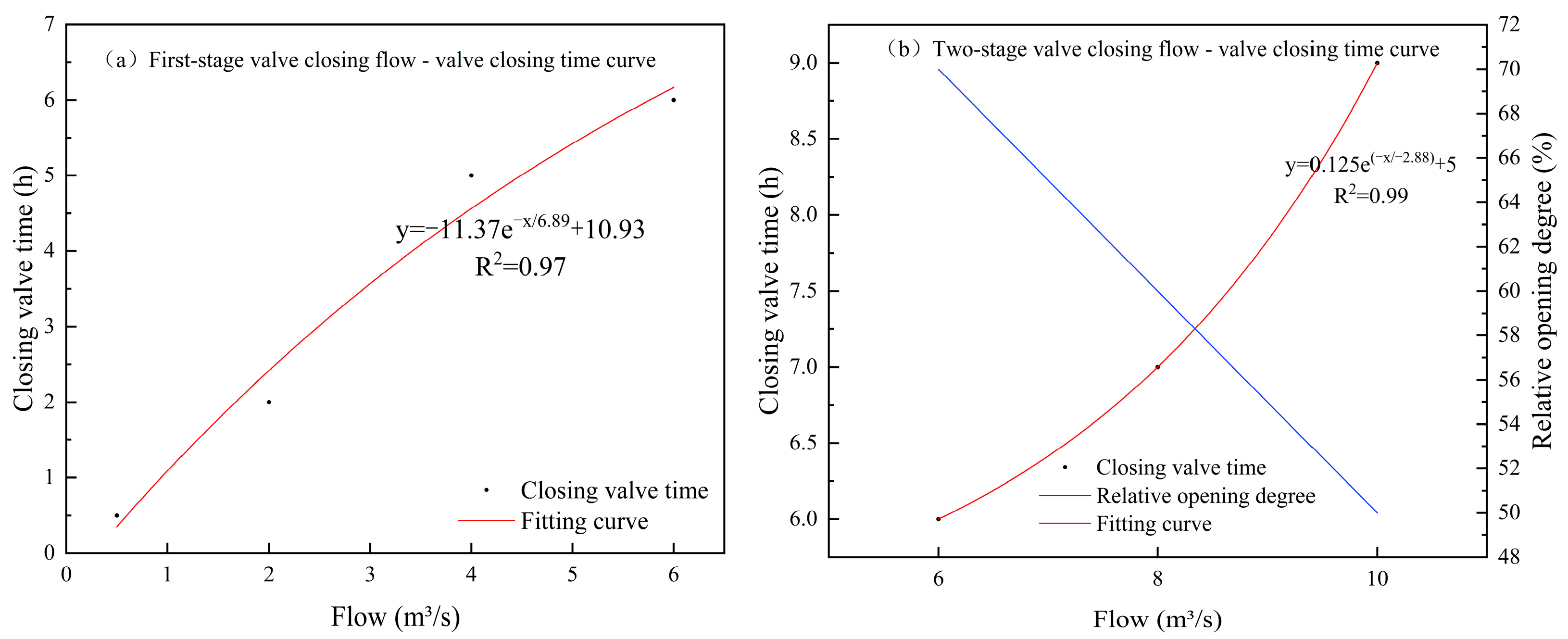
Based on the simulation results, the relationship between pipeline flow rate and valve closure time was fitted to form a curve, as shown in Figure 15.

Figure 15. Flow-off valve time fitting curve diagram.

Figure 15a indicates that when the pipeline flow rate ranges from 0.5 to 6.0 m³/s, a single-stage valve closure can be used based on the flow rate. Figure 15b shows that when the flow rate is between 6.0 and 10.0 m³/s, a two-stage valve closure is recommended. By selecting the appropriate fast closure angle according to the flow rate, valve closure time can be reduced.

4. Discussion

This study addresses the high-gradient characteristics of self-pressurized irrigation networks by establishing a dynamic coordinated mechanism between valve operation rules and groups of air release and vacuum valves. In terms of protective device optimization, unlike traditional valve layout methods based on empirical formulas, a valve group configuration method based on critical flow velocity is proposed. The research shows that by installing a reinforced valve group (a combination of 5 + 3 valves) at the inlet bend, combined with uniformly distributed valves, negative pressure along the entire pipeline can be eliminated with only 14 air release and vacuum valves. This is a significant improvement compared to similar large-scale water conveyance projects in Africa, which require 36 composite air valves [17]. This method reduces the number of devices while ensuring effective protection. By optimizing the air release process through gas–liquid exchange boundary equations, it helps mitigate secondary water hammer risks caused by high-speed air discharge from traditional air valves. Regarding valve operation strategy, this study proposes a flow-adaptive valve closure mechanism: linear closure is used when the flow rate is below 6 m³/s, while a two-stage closure is required when the flow exceeds this threshold. As flow increases, the fast-closure angle dynamically decreases from 70% to 50%. This finding offers a new approach to controlling negative pressure in vulnerable sections at the pipeline inlet of long-distance gravity flow systems. Compared to the fixed valve closure scheme proposed by Yuan L [34] for inlet and outlet valves—where a two-stage fast closure at 75% over 400 s was applied at the inlet and an 85% fast closure over 600 s at the outlet—their study highlighted the critical influence of valve location on water hammer protection but did not account for the dynamic demands caused by periodic flow fluctuations in actual irrigation systems. In contrast, this study establishes a quantified regulation between flow rate and valve closure parameters, achieving for the first time an adaptive valve closure strategy that responds dynamically to operating conditions. Notably, in the vulnerable inlet zone, this study confirms that reducing the fast-closure angle to 50% under high-flow conditions effectively suppresses negative-pressure risks, addressing the flow adaptability limitations of Yuan Lin’s approach. Regarding protection efficiency, Yuan Lin’s scheme relies on 54 air release valves for full-line protection, whereas this study’s valve group optimization model based on critical flow velocity requires only 14 air release valves. The strategy of combining reinforced valve groups at the inlet with uniformly distributed valves not only eliminates negative-pressure hazards but also reduces equipment investment costs by 74%. It is important to emphasize that Yuan Lin’s logic of fast closure to eliminate negative pressure and slow control to stabilize positive pressure provides a crucial theoretical reference for optimizing two-stage valve closure parameters in this study. Meanwhile, the flow-segmented control mechanism proposed here paves a new path for upgrading from static valve closure schemes to dynamic, coordinated water hammer prevention strategies.

Compared with existing protection schemes, the coordinated mechanism proposed in this study demonstrates promising application potential in specific scenarios. Unlike the combined “air chamber + overpressure relief valve” solutions commonly used in pump station systems [36], the passive protection system developed in this study is better suited for pure gravity flow scenarios, maintaining pressure within safe thresholds while avoiding reliance on external energy sources. It should be noted that although the one-dimensional transient flow model used here efficiently simulates pressure wave propagation in long-distance pipeline networks, it has inherent limitations in capturing localized vortex structures around bends and valves. In particular, it struggles to accurately depict gas–liquid mixing and vortex core evolution near air release and vacuum valve groups. In contrast, Han et al. [13] investigated water hammer in ball valve pipelines using a three-dimensional CFD approach combined with sliding mesh technology and the SST k-ω turbulence model. Their study revealed the spatiotemporal evolution of vortex core structures during valve closure and how these structures modulate pressure oscillations. Specifically, Han’s research confirmed that the high-flow velocities during the fast-closure phase significantly intensify vortex core strength and induce high-frequency pressure pulsations. This finding provides a three-dimensional flow field perspective explaining the fundamental cause of the phenomenon observed in this study—“excessively large fast closure angles aggravating negative pressure at the pipeline inlet”—attributed to energy dissipation imbalances caused by local vortices. It is important to emphasize that these two methods have distinct application boundaries: the one-dimensional model offers computational efficiency advantages for system-level pressure wave propagation simulations, while the CFD approach is irreplaceable for detailed device-level flow mechanism analysis. Therefore, future research could integrate the one-dimensional pipeline network model developed here with Han’s fine-scale three-dimensional valve domain simulations to build a system-local multi-scale coupling framework. This integrated approach would more comprehensively reveal the interaction mechanisms between water hammer waves and vortices in high-gradient irrigation pipeline networks.

5. Conclusions

This study establishes a one-dimensional finite-difference water hammer simulation framework for gravity-fed irrigation systems, integrating axial unconstrained conditions and hydraulic resistance to accurately characterize pressure-wave propagation in long-distance self-pressurized pipelines. System simulations of a representative large-scale network reveal that an optimized air valve configuration significantly enhances protection efficiency. Specifically, deploying a reinforced five-valve cluster at inlet bend station K0+066 and a three-valve cluster at station K0+562, complemented by individual downstream valves spaced at 1100 m intervals, completely mitigates system-wide negative pressure. This targeted 14-device layout achieves a 74% reduction in equipment investment costs compared to traditional empirical designs. Furthermore, a flow-adaptive valve closure strategy is proposed to govern transient dynamics. For flow rates up to 6.0 m³/s, a 6.0 h single-stage linear closure guarantees safe operation. Conversely, discharges ranging from 6.0 to 10.0 m³/s necessitate a two-stage closure mechanism featuring a rapid initial phase over the first third of the operational duration. Within this higher flow regime, dynamically restricting the fast-closure angle from 70% to 50% while simultaneously extending the total closure time from 6.0 to 9.0 h is imperative for suppressing inlet negative pressure and controlling transient fluctuations. The obtained results are well aligned with existing experimental and numerical findings.

Overall, this study proposes a coordinated optimization strategy integrating valve operational control and protective device configuration for water hammer mitigation in gravity irrigation systems, providing a technically robust and practically applicable framework for the design and operation of large-scale self-pressurized irrigation pipelines. However, while the proposed one-dimensional finite difference framework is computationally efficient and technically sound for simulating long-distance pipelines, reliance on a one-dimensional approach inherently limits the model’s ability to fully capture complex three-dimensional flow effects, local turbulence, and structural interactions in large-scale networks. Therefore, future research will aim to integrate the current network model with three-dimensional computational fluid dynamics (CFD) to build a multi-scale coupling framework, thereby more comprehensively revealing the interaction mechanisms between water hammer waves and localized vortices in high-gradient irrigation systems.

References

- Eurasian Development Bank. Efficient Irrigation and Water Conservation in Central Asia; EDB Analytical Report No. 4; Eurasian Development Bank: Almaty, Kazakhstan, 2023; pp. 1–88. Available online: https://eabr.org/en/analytics/special-reports/efficient-irrigation-and-water-conservation-in-central-asia/ (accessed on 3 March 2026).
- Dankova, R.; Burton, M.; Salman, M.; Clark, A.K.; Pek, E. Modernizing Irrigation in Central Asia: Concepts and Approaches; FAO: Rome, Italy, 2022; pp. 1–90. [Google Scholar] [CrossRef] [Scilit]
- Wang, Y.Y.; Long, A.H.; Deng, X.Y.; Abulizi, A.; Wang, J.; Zhang, P.; Hai, Y.; Ren, C.; Zhang, J.; Liu, Y.D.; et al. Spatiotemporal changes and influencing factors of the intensity of agricultural water footprint in Xinjiang, China. Int. J. Agric. Biol. Eng. 2023, 16, 262–272. [Google Scholar] [CrossRef] [Scilit]
- Wang, Z.H.; Chen, X.G.; Zheng, X.R.; Fan, W.B.; Li, W.H.; Zong, R. Discussion of the future development of field drip irrigation in China. Agric. Res. Arid Areas 2020, 38, 1–9. [Google Scholar] [CrossRef]
- Kandil, M.; Kamal, A.M.; El-Sayed, T.A. Effect of pipe materials on water hammer. Int. J. Press. Vessel. Pip. 2020, 179, 103996. [Google Scholar] [CrossRef] [Scilit]
- Wan, W.; Zhang, B.; Chen, X. Investigation on water hammer control of centrifugal pumps in water supply pipeline systems. Energies 2018, 12, 108. [Google Scholar] [CrossRef] [Scilit]
- Zhang, H.Z.; Li, Y.H.; Jiang, J.; Wang, Y.C.; Luo, S. The influence of filling flow discharge on hydraulic performance of hump pipe with air valve. China Rural. Water Hydropower 2019, 11, 172–176. [Google Scholar]
- Arefi, M.H.; Ghaeini-Hessaroeyeh, M.; Memarzadeh, R. Numerical modeling of water hammer in long water transmission pipeline. Appl. Water Sci. 2021, 11, 147. [Google Scholar] [CrossRef] [Scilit]
- Wu, Y.; Liu, M.; Liu, Z.; Zhang, Y.; Mei, J.; Rong, Z. Research on the pipe burst transient progress and valve closure law of long—Distance and gravity flow water supply system. China Rural Water Hydropower 2019, 7, 119–123. [Google Scholar]
- Qiao, H.B.; Zhao, L.; Liu, J.; Yao, X.T.; Qi, Y.Y. Water hammer prevention design of short distance transmission with high pressure pipeline. Water Wastewater Eng. 2019, 37, 160–162. [Google Scholar]
- Li, X.; Wang, T.; Zhang, Y.; Guo, P. Study on the factors influencing air valve protection against water hammer with column separation and rejoinder. J. Water Supply Res. Technol. AQUA 2022, 71, 949–962. [Google Scholar] [CrossRef] [Scilit]
- Wang, L.; Wang, Z. Effect of combination vacuum relief and air release valve on hydraulic transients during pipeline filling process. IOP Conf. Ser. Earth Environ. Sci. 2019, 240, 052032. [Google Scholar] [CrossRef] [Scilit]
- Han, Y.; Shi, W.; Xu, H.; Wang, J.; Zhou, L. Effects of closing times and laws on water hammer in a ball valve pipeline. Water 2022, 14, 1497. [Google Scholar] [CrossRef] [Scilit]
- Wu, L.; You, R.; Wang, W.; Zhang, F. Status of research on water hammer effect in long-distance pressure pipelines. J. Eng. Res. Rep. 2022, 23, 204–211. [Google Scholar] [CrossRef] [Scilit]
- Tang, Y.; Cheng, Y.; Shen, L.; Wu, J.; Zhang, Y.; Li, Q.; Yuan, L. Analysis of the effectiveness of water hammer protection programs for complex long-distance and high-head water supply projects. Water 2024, 16, 1582. [Google Scholar] [CrossRef] [Scilit]
- Wang, Z.P.; Jia, D.Y.; Ma, Z. Optimization of Valve Closing Scheme for Long-Distance Gravity Flow Water Delivery Project. Yellow River 2021, 43, 142–146. [Google Scholar] [CrossRef]
- Bergant, A.; Simpson, A.R.; Tijsseling, A.S. Water hammer with column separation: A historical review. J. Fluids Struct. 2006, 22, 135–171. [Google Scholar] [CrossRef] [Scilit]
- Meniconi, S.; Brunone, B.; Ferrante, M.; Mazzetti, E.; Laucelli, D.B.; Massari, C. Transient effects of self-adjustment of pressure reducing valves. Procedia Eng. 2015, 119, 1030–1038. [Google Scholar] [CrossRef] [Scilit]
- Vítkovský, J.P.; Bergant, A.; Simpson, A.R.; Lambert, M.F. Systematic Evaluation of One-Dimensional Unsteady Friction Models in Simple Pipelines. J. Hydraul. Eng. 2006, 132, 696–708. [Google Scholar] [CrossRef] [Scilit]
- Duan, H.-F.; Ghidaoui, M.S.; Lee, P.J.; Tung, Y.-K. Relevance of unsteady friction to pipe size and length in pipe fluid transients. J. Hydraul. Eng. 2012, 138, 257–268. [Google Scholar] [CrossRef] [Scilit]
- Tijsseling, A.S. Fluid–structure interaction in liquid-filled pipe systems: A review. J. Fluids Struct. 1996, 10, 109–146. [Google Scholar] [CrossRef] [Scilit]
- Neyestanaki, M.K.; Dunca, G.; Jonsson, P.; Cervantes, M.J. A comparison of different methods for modelling water hammer valve closure with CFD. Water 2023, 15, 1510. [Google Scholar] [CrossRef] [Scilit]
- Martins, N.M.C.; Soares, A.K.; Ramos, H.M.; Covas, D. CFD modeling of transient flow in pressurized pipes. Comput. Fluids 2016, 126, 129–140. [Google Scholar] [CrossRef] [Scilit]
- Cao, Y.; Zhou, L.; Ou, C.; Fang, H.; Liu, D. 3D CFD simulation and analysis of transient flow in a water pipeline. J. Water Supply Res. Technol. AQUA 2022, 71, 751–767. [Google Scholar] [CrossRef] [Scilit]
- Al-Azawy, M.G.; Turan, A.; Revell, A. An overset mesh approach for valve closure: An LVAD application. In Proceedings of the 9th International Joint Conference on Biomedical Engineering Systems and Technologies (BIOSTEC 2016), Rome, Italy; SciTePress: Setúbal, Portugal, 2016; pp. 145–151. [Google Scholar] [CrossRef] [Scilit]
- Kumar, M.R.A.; Bornoff, J.; Narayan, P.A.; Revell, A. Insights into CFD modelling of water hammer. Water 2023, 15, 3988. [Google Scholar] [CrossRef] [Scilit]
- Tang, Z.R.; Zhang, B.Y.; Jiang, J.; Liao, Z.F.; Li, Y.H. Cavitating flow characteristic analysis of flow and pressure regulating valve with piston. J. Hydroelectr. Eng. 2021, 40, 50–58. [Google Scholar]
- Zhu, H.Y. Optimization selection of water hammer protection measures for a water conveyance system in Africa. Eng. Des. 2018, 13, 169–170. [Google Scholar] [CrossRef]
- Wang, P. Study on Pump-Stopping and End of Branch Pipeline Valve-Closure Water Hammer of Ring Water Transmission Network. Master’s Thesis, Chang’an University, Xi’an, China, 2020. [Google Scholar]
- Toumi, A.; Sekiou, F. Optimal valve closing law for improved water hammer control: A case from a water supply pipeline in Guelma, Algeria. Aqua Water Infrastruct. Ecosyst. Soc. 2024, 73, 200–216. [Google Scholar] [CrossRef] [Scilit]
- Li, K.; Wu, J.; Liu, Y.; Guo, W.; Sun, Y.; Han, Y. Research on effect of protection against water hammer of air vessel in pumping station. Yangtze River 2020, 51, 200–204. [Google Scholar] [CrossRef]
- Wang, Q.; Li, Z.; Zhu, C.; Li, H. Water hammer control in gravity flow pipeline based on double-valve regulation. China Water Wastewater 2020, 36, 52–58. [Google Scholar] [CrossRef]
- Zhao, Z.; Zhao, X.; Wan, J.; Jiang, J. Study on water hammer protection of long-distance pressurized water conveyance system based on method of characteristics. Water Wastewater Eng. 2019, 45, 277–280. [Google Scholar] [CrossRef]
- Yuan, L.; Li, Y.; Kou, Z. Optimization of valve at both ends closing scheme for long-distance gravity flow water conveyance project. Water Resour. Power 2022, 40, 118–121. [Google Scholar]
- Wang, Y. Study on Water Hammer and Its Protection in Water Transportation System of Mountainous Urban; Chongqing University: Chongqing, China, 2018. [Google Scholar]
- Bai, M.M.; Wang, F.J.; Lei, C.; Wang, L.; Liu, B.C. Effect of bypass valve on hydraulic transient process in long water transport pipelines with gravity flow. J. Drain. Irrig. Mach. Eng. 2019, 37, 58–62. [Google Scholar] [CrossRef]
- Li, N.; Zhang, J.; Shi, L.; Chen, X.Y.; Zhang, X.Y. Water hammer protection characteristic of combined air vessel and overpressure relief valve. J. Drain. Irrig. Mach. Eng. 2020, 38, 254–260. [Google Scholar] [CrossRef]
- Yazdi, J.; Hokmabadi, A.; JaliliGhazizadeh, M.R. Optimal size and placement of water hammer protective devices in water conveyance pipelines. Water Resour. Manag. 2018, 33, 569–590. [Google Scholar] [CrossRef] [Scilit]
- Wang, J.; Ma, P.A.; Cui, H.J.; Zhao, H.L. Design of long-distance gravity conveyance pipeline for a water diversion project in Xi’an. China Water Wastewater 2021, 37, 84–88. [Google Scholar] [CrossRef]
- Ghidaoui, M.S.; Zhao, M.; McInnis, D.; Axworthy, D. A review of water hammer theory and practice. Appl. Mech. Rev. 2005, 58, 49–76. [Google Scholar] [CrossRef] [Scilit]
- Tijsseling, A.S. Water hammer with fluid–structure interaction in thick-walled pipes. Comput. Struct. 2007, 85, 844–851. [Google Scholar] [CrossRef] [Scilit]
- Zielke, W. Frequency-dependent friction in transient pipe flow. ASME J. Basic Eng. 1968, 90, 109–115. [Google Scholar] [CrossRef] [Scilit]
- American Water Works Association (AWWA). M51: Air Valves—Air Release, Air/Vacuum, and Combination, 2nd ed.; AWWA: Denver, CO, USA, 2016. [Google Scholar]
- Wylie, E.B.; Streeter, V.L. Fluid Transients in Systems; Prentice Hall: Englewood Cliffs, NJ, USA, 1993. [Google Scholar] [CrossRef] [Scilit]
Disclaimer/Publisher’s Note: The statements, opinions and data contained in all publications are solely those of the individual author(s) and contributor(s) and not of MDPI and/or the editor(s). MDPI and/or the editor(s) disclaim responsibility for any injury to people or property resulting from any ideas, methods, instructions or products referred to in the content. |
© 2026 by the authors. Licensee MDPI, Basel, Switzerland. This article is an open access article distributed under the terms and conditions of the Creative Commons Attribution (CC BY) license.