


Abstract
Accurate prediction of outflow sediment transport rates in sediment-laden rivers underpins sediment load calculations, reservoir sedimentation analysis, and water-sediment regulation. The cascade reservoir water and sediment state-guided Informer (crsg-informer) is proposed to improve the representation of antecedent sediment supply and reservoir storage–release processes. It also addresses high-sediment peak underestimation and declining prediction accuracy at longer lead times. Daily changes, antecedent cumulative values, and rolling peaks enhance process features, while numerical water and sediment variables, historical positions, and water and sediment phases are encoded separately. A hierarchical weighted Huber regression loss and auxiliary high-sediment-state classification strengthen learning from high values. Using Sanmenxia (SMX) and Xiaolangdi (XLD) reservoirs as examples, daily data from 2002–2022 are analysed with a 30 d historical window. Outflow sediment transport rates are predicted at 1, 3, 5, and 7 d under the given water-sediment and operating information. Predictions are compared with those of seven models, and module ablations assess the contribution of each improvement. The results show that CRSG-Informer improves multistep predictions for both reservoirs. At 7 d, root mean square error (RMSE) decreases by 11.87% and 18.52%, respectively, relative to the best benchmark at that lead time. The annual observed peak recovery ratio (PR) is closer to 100% in 11 of 12 annual peak scenarios. SMX benefits more from process feature enhancement, with improvements concentrated on rapid sediment rises and peak recovery. XLD benefits more from auxiliary high-sediment-state classification, with improvements covering concentrated sediment peaks and post-peak recession under sustained storage–release conditions. The results indicate that jointly representing historical water-sediment processes and operating conditions, and strengthening learning from infrequent high-value samples, helps reduce magnitude biases during critical sediment transport phases. This reduces their contribution to errors in sediment load calculations.
1. Introduction
Sediment transport in cascade reservoirs in sediment-laden rivers is relevant to reservoir capacity maintenance, channel evolution, and water-sediment regulation [1,2]. Reservoir sediment trapping and water-sediment regulation alter sediment transport processes [3,4]. Cascade operation makes sediment outflow dependent on upstream sediment supply, reservoir regulation and storage, and antecedent water-sediment states [5,6]. A small number of high-sediment days account for substantial sediment loads, while underestimation of sediment peaks may reduce calculated cumulative sediment loads and affect comparisons of sediment release schemes. Accurate prediction of outflow sediment transport rates over the following few days thus underpins sediment load calculations and water-sediment regulation in cascade reservoirs.
Sediment transport rate prediction mainly uses physical models, empirical formulas, machine learning, and deep learning methods. Physical models simulate sediment transport through equations describing hydrodynamics, sediment transport, and riverbed deformation [7]. Wu [8] developed a two-dimensional hydrodynamic model for nonuniform sediment to calculate channel sediment transport and riverbed scour and deposition. Wang et al. [9] developed a finite-volume river network model, improving sediment transport simulations of hyperconcentrated floods at confluences. Xia et al. [10] coupled one-dimensional water and sediment modules with an operation module to simulate sediment transport, scour, and deposition in the Sanmenxia (SMX)–Xiaolangdi (XLD) reservoir–river system. Empirical methods derive formulas from observed water–sediment relationships to simplify sediment transport calculations [11,12]. Yang et al. [13] modified the unit stream power formula, improving bed-material sediment transport calculations under hyperconcentrated conditions in the Yellow River. Xu [14] developed a flood sediment delivery ratio relationship to identify scour–deposition thresholds in the lower Yellow River. Cheng et al. [15] modified parameters in a sediment transport capacity formula, improving sediment transport and scour–deposition calculations for flows with low sediment concentrations. Mechanistic models depend on cross-section and boundary data, whereas the applicability of empirical relationships is constrained by water and sediment conditions [16]. Data-driven methods have therefore developed progressively. Kakaei Lafdani et al. [17] developed artificial neural network (ANN) and support vector machine (SVM) models with input selection to improve daily sediment load prediction. Ensemble models help improve the stability of sediment predictions [18,19]. Tan et al. [20] coupled physical processes with machine learning, reducing sedimentation simulation errors in cascade reservoir systems. Hydroclimatic variables, lag selection, and feature interpretation have expanded the information used by models [21,22]. Hemmatzadeh et al. [23] embedded sediment rating curve constraints and an asymmetric loss in extreme gradient boosting (XGBoost), improving extreme-value and multistep predictions. Decomposition-based preprocessing has improved the representation of nonstationary water and sediment processes [24,25]. Historical dependence in water-sediment processes has driven dynamic sequence modelling. Deep temporal models further learn long-term relationships in continuous water and sediment processes [26]. Kaveh et al. [27] developed a long short-term memory (LSTM) model, improving the accuracy of daily sediment concentration and cumulative sediment load calculations. Jamei et al. [28] proposed an encoder–decoder bidirectional LSTM model driven by decomposition and feature selection to improve nonstationary daily sediment load prediction. Attention models have subsequently been introduced for long-sequence forecasting. Zhou et al. [29] proposed Informer, reducing the computational cost of long-sequence forecasting through sparse attention and distillation. Fan et al. [30] coupled decomposition with a convolutional Transformer, improving joint modelling of local sediment concentration fluctuations and long-term dependencies. Liu et al. [31] proposed an Informer model with dimension-segmented embeddings (Heformer), improving the accuracy of reservoir operation rule extraction. However, targeted representations of cascade processes still require refinement. Ribeiro and Moniz [32] proposed target-relevance-driven evaluation and optimisation using the squared error-relevance area (SERA), strengthening extreme-value learning in imbalanced regression. However, prediction accuracy for scarce high-sediment samples remains limited. Overall, existing methods still have three limitations in sediment transport rate prediction for cascade reservoirs. Antecedent sediment supply and target-reservoir regulation and storage information are insufficiently used, while operating states and water and sediment phases remain inadequately represented. Low-sediment samples dominate, and high-sediment processes are prone to underestimation, leaving room to improve overall accuracy and sediment peak recovery [33]. Prediction accuracy remains prone to deterioration at longer lead times [34,35].
To address these issues, this study proposes the cascade reservoir water and sediment state-guided Informer (CRSG-Informer) with three improvements. First, historical sequences from upstream stations and reservoirs and the target reservoir are supplemented with daily changes, antecedent cumulative values, and rolling peaks. These features supplement sediment supply and regulation information, converting antecedent sediment supply and regulation processes into effective features. Second, numerical water and sediment variables, temporal positions, and water and sediment phases are encoded separately. This provides more detailed representations of operating states and water and sediment phases, improving prediction accuracy at longer lead times. Third, auxiliary high-sediment-state classification and a hierarchical weighted Huber loss strengthen learning from infrequent high-value samples and alleviate sediment peak underestimation. The model retains sparse attention, a single-layer encoder, and self-attention distillation, producing predictions for multiple lead times in one pass. Using SMX and XLD reservoirs as examples, 30 d of historical data are used to predict outflow sediment transport rates at 1, 3, 5, and 7 d. These measures were evaluated using composite indicators, process curves, peak recovery performance, and reduction experiments, providing a basis for predicting sediment load and water-sediment regulation in cascade reservoirs.
2. Methods
2.1. Informer Model
Informer is an encoder–decoder model for long-sequence forecasting, comprising an input layer, an encoder layer, and a generative decoder. The encoder layer includes ProbSparse attention and self-attention distillation. Sparse attention extracts relationships between historical positions, distillation compresses the temporal dimension, and the decoder outputs the future sequence in one pass. This reduces error accumulation caused by recursive prediction [29].
2.1.1. Input Representation Layer
Let denote the forecast issue date, the historical window length, and the input feature column vector on day . The historical input matrix is obtained by arranging these vectors chronologically over consecutive days:
where is the historical input matrix, and is the daily feature vector; is set to 30 d, and denotes transposition.
The original Informer adds value embeddings, positional encodings, and temporal embeddings to form the input representation [29]. Value embeddings map observed variables through a one-dimensional convolution, while sinusoidal encodings represent positions within the window. Temporal embeddings, including month, day, and day of the week, provide calendar context. These three embeddings share the same dimension and represent numerical states, sequence order, and temporal information, respectively.
2.1.2. Encoder Layer
(1) ProbSparse multi-head attention
The encoder uses self-attention to extract correlations between historical positions. Linear mappings transform the input representation into a query matrix , a key matrix , and a value matrix . Query–key matching scores determine the information weight assigned to each position. Scaled dot-product attention is expressed as follows:
where , , and are the query, key, and value matrices, respectively, and is the dimension of each head. normalises matching scores across key positions.
Full attention computes matching scores for all queries and keys. ProbSparse samples keys to calculate query sparsity and computes full attention only for queries with large differences between maximum and mean scores. The remaining queries use a simplified context to reduce computation. Its time and memory complexity grows approximately with the product of sequence length and its logarithm [29]. Each attention head extracts relationships in a different feature space. Concatenated outputs are updated through linear mapping, residual connections, layer normalisation, and a feedforward network (FFN).
(2) Self-attention distillation
Self-attention distillation aggregates information from neighbouring time steps through convolution and pooling, compressing the temporal dimension while retaining major historical features [29]. Distillation uses one-dimensional convolution (Conv1d), exponential linear unit (ELU) activation, and max pooling (MaxPool). In this study, Informer and CRSG-Informer both use a single encoder layer followed by one distillation operation:
where is the encoder output, and is the distillation result. comprises Conv1d, ELU activation, and MaxPool, with a convolution kernel width of 3 and a pooling stride of 2.
The distilled output aggregates neighbouring time steps and no longer corresponds day-by-day to the original 30 d sequence.
2.1.3. Generative Decoder
The original Informer decoder uses known historical targets as starting information, followed by a zero-valued placeholder sequence for the future period [29]:
where is the decoder input, contains known historical targets, and contains zero-valued placeholders for the forecast period. denotes temporal concatenation; temporal embeddings provide future calendar information.
The original decoder processes inputs through causally masked self-attention, cross-attention, and an FFN. The causal mask prevents each position from accessing subsequent decoder positions, while cross-attention extracts historical information from the encoded representation. A final linear projection outputs the future sequence. For the four fixed lead times considered here, a direct multistep prediction head outputs the corresponding sediment transport rates.
2.2. CRSG-Informer Model
To accommodate sediment transport characteristics in cascade reservoirs, CRSG-Informer retains ProbSparse encoding and self-attention distillation. It adds cascade process features, hybrid embeddings of hydrological information, and high-sediment-state training. These improvements respectively supplement antecedent water and sediment processes, distinguish numerical and temporal information, and strengthen learning from infrequent high-sediment samples.
2.2.1. Cascade Process Features
The target reservoir is denoted by , and upstream stations and reservoirs by and . SMX uses data from Longmen, Tongguan, and SMX itself; XLD uses data from Tongguan, SMX, and XLD itself. Models are trained separately for the two reservoirs, using only historical information observed by the forecast issue time.
Single-day observations cannot fully reflect the effects of antecedent sediment supply and reservoir regulation and storage. Daily changes, antecedent cumulative features, and rolling peaks are therefore constructed for applicable continuous variables to supplement historical water and sediment states:
where is the observed value on day , and denotes the change between two consecutive days.
where is the sum of observations over the preceding days; is set to 3, 7, or 15 d, and is the look-back duration.
where is the maximum observation over the preceding days; the peak window is set to 7 d.
Flow and sediment transport rate are expressed in m3/s and t/s, respectively. Cumulative windows are 3, 7, and 15 d, and the peak window is 7 d. Sums of daily mean rates serve as statistical features of antecedent supply. Conversion to water volume or sediment load requires multiplication by the number of seconds in a day. Reservoir water level is represented by its original value and daily change, in m. Original variables and process features jointly form the daily inputs. Each feature uses only data available on or before the forecast issue date and is standardised using training-set statistics.
2.2.2. Hybrid Embeddings of Hydrological Information
Continuous water and sediment variables reflect numerical states, while window positions indicate the temporal relationship between observations and the forecast issue date. Month, flood-season phase, and water and sediment phase labels jointly provide calendar and operating context. This information is separately encoded as value, positional, and phase embeddings and mapped to the same hidden dimension.
where is the value embedding, and are trainable parameters, and contains the input features at that position. The embedding dimension is set to 20.
where is the positional embedding, and is the sinusoidal encoding of historical position , with a dimension of 20.
where is the phase embedding; , , and denote month, flood-season phase, and water and sediment phase labels, respectively. Their numbers of categories are 12, 2, and 2, respectively; each label embedding table has an output dimension of 20.
Based on the annual hydrological and operating context of the Yellow River, this study defines 12 month labels. Two flood-season phase labels distinguish the flood season, from 1 July to 1 November each year, from all other days. Two water and sediment phase labels distinguish the water-sediment regulation period, from 1 July to 10 August, from all other days. XLD, the outlet of the studied cascade, is a key facility for water-sediment regulation on the Yellow River. The water-sediment regulation period label was therefore based mainly on observed daily outflow sediment transport rates at XLD. The window covers approximately 11.2% of the days in a year and accounts for 86.4% of the cumulative outflow sediment load at XLD during 2002–2022. The same label window is used for SMX. All labels are assigned by date, using the same rules for training, validation, and testing.
The three embeddings are integrated using learnable weights, allowing training to adjust the relative contributions of numerical, positional, and phase information:
where is the integrated representation; , , and are the weights of the three embeddings. The three fusion weights are initialised equally, updated through backpropagation during training, and normalised using softmax.
2.2.3. High-Sediment-State Training
Sediment transport rate samples are dominated by low and zero values, making equally weighted training prone to underestimating infrequent high-sediment processes. The 75th percentile (P75) and 90th percentile (P90) of positive training-set sediment transport rates are used to distinguish normal, high-sediment, and very-high-sediment states. This increases the training contribution of high-value samples. Validation and testing use the same two thresholds. The normal state includes zero values and positive values not exceeding P75.
For a training target with forecast issue date and lead time , the sample weight is defined piecewise:
where is the target-day observation, is the lead time, and is the sample weight. and are the thresholds defined above, while , , and are the three state weights. Specific parameter values are provided in Section 3.2.
An auxiliary high-sediment-state classification task is added to help the shared encoder identify high-sediment states. The threshold is P75 of positive training-set sediment transport rates for each reservoir. The target-day label is 1 when its sediment transport rate exceeds this threshold and 0 otherwise. Validation and testing use the same training-set threshold. The classification and regression heads share a hidden representation, with high-sediment labels providing additional state supervision. During training, the auxiliary high-sediment-state classification loss is multiplied by its coefficient and added to the joint loss, providing additional high-sediment-state supervision.
2.2.4. Model Training and Prediction
(1) Prediction outputs
The model comprises a shared encoder, a regression head, and an auxiliary high-sediment-state classification head. The historical sequence with hybrid embeddings first passes through a single ProbSparse multi-head encoder layer:
where is the single-layer encoder. Its output is distilled into using Equation (3) and shared by the regression and classification heads.
where is the regression head, and is the prediction vector ordered by lead times of 1, 3, 5, and 7 d. An asterisk denotes the standardised scale, and a hat denotes a predicted value.
where is the classification head, and contains high-sediment probabilities at the four lead times. maps outputs to the range 0–1; outputs for each lead time are denoted by and .
(2) Standardisation and training loss
Training errors are calculated on the standardised scale so that sediment transport rate magnitudes do not directly determine the loss. Observed targets are standardised using the training-set mean and standard deviation:
where is the standardised target, and and are the training-set mean and standard deviation, also used for validation and testing. The difference between predicted and observed values is denoted by .
The loss is used to balance the fitting of small residuals with stability for large residuals:
where is the piecewise threshold, set to 0.70. Small residuals use a quadratic loss, whereas large residuals use a linear loss.
The regression loss is the mean hierarchical weighted loss across targets within a batch, with each target assigned weight . The auxiliary high-sediment-state classification loss uses the mean binary cross-entropy (BCE) between state labels and predicted probabilities . The joint training objective is expressed as follows:
where is the joint loss, and is the auxiliary high-sediment-state classification loss coefficient. Both losses are averaged over batch samples and the four lead times.
(3) Direct multistep prediction
The model uses direct multistep prediction, with each output corresponding to one target date. At prediction time, 30 d of historical data available through the forecast issue date undergo feature construction, embedding, encoding, and distillation. Target values for 1, 3, 5, and 7 d are output in one pass and inverse-standardised to obtain actual sediment transport rates:
where is the sediment transport rate predicted on issue date for target date , expressed in t/s.
2.2.5. CRSG-Informer Workflow
The CRSG-Informer workflow is shown in Figure 1. From left to right, the model performs input processing, embedding, encoding, distillation, and prediction. The dashed path at the bottom indicates parameter updates based on the joint loss. The specific steps are described below.
Figure 1.
CRSG-Informer workflow for sediment transport rate prediction.
(1) Multisource inputs
Historical water and sediment data are collected from upstream stations and reservoirs and and the target reservoir . Daily changes, antecedent cumulative values, and rolling peaks are constructed to form the 30 d historical inputs. Month, flood-season phase, and water and sediment phase labels are also prepared. These correspond to the water and sediment sequence inputs and external temporal and phase information in the figure.
(2) Embedding layer
Water and sediment features, historical positions, and month, flood-season phase, and water and sediment phase labels are converted into value, positional, and phase embeddings, respectively. These embeddings are then integrated into a unified sequence representation, corresponding to the three embedding modules and their convergence in the figure.
(3) Single-layer encoding and self-attention distillation
The integrated sequence passes through ProbSparse multi-head self-attention and an FFN, with residual connections and layer normalisation extracting historical features. Conv1d, ELU activation, and MaxPool then compress the temporal dimension and produce the distilled representation .
(4) Dual-head prediction outputs
The hidden representation is passed simultaneously to the multistep regression head and the auxiliary high-sediment-state classification head. The regression head outputs sediment transport rate predictions at 1, 3, 5, and 7 d in one pass. The classification head outputs high-sediment probabilities for the corresponding lead times, forming the two prediction branches on the right.
(5) Joint loss and model training
During training, the hierarchical weighted loss evaluates sediment transport rate predictions, and BCE evaluates auxiliary high-sediment-state classification. They are combined into the joint loss using coefficient .
(6) Forecast outputs
After training, prediction follows the forward path at the top of Figure 1. Regression outputs are inverse-standardised to obtain actual sediment transport rates at the four lead times.
2.3. Model Evaluation Metrics
Overall evaluation uses root mean square error (RMSE), Nash–Sutcliffe efficiency (NSE), squared Pearson correlation coefficient (R2), and Kling–Gupta efficiency (KGE). High-sediment evaluation uses the annual observed peak recovery ratio (PR). It also uses mean recovery ratios on days with the 5 and 10 highest observed sediment transport rates, termed Top5 and Top10 recovery ratios. It also uses RMSE for continuous high-sediment events.
2.3.1. Overall Prediction Metrics
Overall performance is evaluated using , , , and , calculated separately for each reservoir, dataset, and lead time. Observations and predictions are paired by target date and denoted by and ; is the sample index, and is the sample size.
(1) RMSE
where and are paired observations and predictions, and is the sample size. is expressed in t/s, with smaller values indicating smaller errors.
(2) NSE
where is the observed mean. Values of closer to 1 indicate more accurate predictions relative to the mean benchmark.
(3) R2
The Pearson correlation coefficient describes the linear correlation between observed and predicted sequences. Its squared value, reported in the results figures and tables, is:
where is the Pearson correlation coefficient between observed and predicted sequences, and is its squared value.
(4) KGE
jointly considers correlation, variability, and mean differences and is expressed as follows:
where and are the observed and predicted standard deviations, respectively, and is the predicted mean. Values of closer to 1 indicate better overall agreement.
2.3.2. High-Sediment Process Evaluation Metrics
, and recovery ratios, and continuous high-sediment event evaluate annual peaks, high-value-day magnitudes, and continuous process errors, respectively. These four metrics are used for performance analysis after training, rather than as training losses or criteria for hyperparameter selection. Each metric is calculated separately for each reservoir and lead time, pairing observations and predictions for the same target date.
(1) PR
PR evaluates magnitude recovery on infrequent high-sediment days. For each reservoir, year, and lead time, the maximum observed sediment transport rate and the prediction for the same peak day are identified:
where is the annual maximum observed sediment transport rate, and is the prediction for the same peak day. The ideal recovery ratio is 100%; values below or above 100% indicate underestimation or overestimation, respectively. Multiyear results are calculated as an equally weighted mean of across valid years.
(2) High-sediment event RMSE
A high-sediment event is triggered when the observed sediment transport rate exceeds of positive training-period values. Its start is traced back to the preceding trough, and it ends after 2 consecutive days at or below the threshold. Multipeak events are divided into their principal pulses. For each pulse, the start, observed peak day, and end are denoted by , , and , respectively, with phases defined as follows:
The set contains valid dates in the rising-sediment, peak-day, and receding-sediment phases of all high-sediment events. High-sediment event RMSE is calculated as follows:
where and are the observed and predicted sediment transport rates at time , respectively, and is the number of valid days in the set.
(3) High-value-day recovery ratios (Top5 and Top10)
Within the evaluation period , the positive-value days with the highest observed sediment transport rates form set . Their recovery ratio is:
where and correspond to values of 5 and 10, respectively; the actual number of days is used when fewer than are available. Recovery ratios closer to 100% are better; values below or above 100% indicate underestimation or overestimation, respectively.
3. Case Study
3.1. Study Area and Datasets
3.1.1. Study Area
The study area lies at the transition between the middle and lower reaches of the Yellow River. The middle Yellow River flows through the Loess Plateau, receiving substantial sediment inputs and exhibiting pronounced variations in water and sediment processes. As the Yellow River enters its lower-course plains, the channel gradient decreases across the lower-reach plain, where sediment deposition and reservoir regulation strongly influence river water and sediment conditions. This study examines SMX and XLD, two cascade reservoirs on the Yellow River mainstem, predicting outflow sediment transport rates at 1, 3, 5, and 7 d. From upstream to downstream, Longmen hydrological station is located at the outlet of the Shanxi–Shaanxi Gorge and reflects middle-mainstem water- sediment inflows. Tongguan hydrological station, near the Wei River confluence with the Yellow River, is an important water and sediment control station upstream of SMX. SMX is downstream of Tongguan, and XLD is downstream of SMX. The study area and the locations of the stations and reservoirs are shown in Figure 2, while Table 1 lists the input stations and prediction targets for both reservoirs.
Figure 2.
Study area and locations of cascade stations and reservoirs.
Table 1.
Input and output information for the two reservoirs.
Table 1 summarises input stations and reservoirs and output lead times for the two reservoirs. Models are trained separately; the XLD model uses historical SMX outflows observed by the forecast issue time, without using future predictions from SMX.
3.1.2. Datasets and Partitioning
Water and sediment data comprise daily flow, sediment transport rate, and water level observations from Longmen and Tongguan hydrological stations and SMX and XLD during 2002–2022. Data were obtained from the Yellow River Conservancy Commission. The periods 2002–2016, 2017–2019, and 2020–2022 were assigned chronologically to training, validation, and testing, respectively, with sample sizes listed in Table 2. The model uses 30 d of historical data available through the forecast issue date to predict outflow sediment transport rates at 1, 3, 5, and 7 d. The XLD model uses only SMX outflows observed by the forecast issue time. All lead times share the same forecast issue samples, with target dates lying within their respective datasets. With a 30 d historical window and a maximum lead time of 7 d, the training set contains 5443 samples. Validation and testing use preceding historical data and are constrained only by prediction boundaries, yielding 1089 and 1090 samples, respectively. None of the data used in this study contain missing values. Zero outflow sediment transport rates accounted for 71.92% and 89.75% of observations at SMX and XLD, respectively, during 2002–2022. The q75/q90 thresholds calculated from positive training-period values were 19.80/70.36 t/s and 26.08/79.15 t/s, respectively. The 5443 training samples per reservoir and lead time comprised 5057/231/155 normal/high-sediment/very-high-sediment samples at SMX and 5330/67/46 at XLD.
Table 2.
Data partitioning and evaluation sample sizes.
The 29 inputs comprise 7 original variables and 22 process features. Original variables include flow and sediment transport rate at each of two upstream locations, plus outflow, outflow sediment transport rate, and water level at the target reservoir. Process features include daily changes in these 7 variables, 3, 7, and 15 d cumulative values for 3 sediment transport rate sequences (9 features). They also include 7 d maxima for 3 flow and 3 sediment transport rate sequences (6 features). All inputs use only observations available on or before the forecast issue date; rolling windows include the current observed day. The 30 d window forms a 30 × 29 input matrix, with standardisation based only on training-set statistics.
3.2. Methods and Parameter Settings
To compare modelling strategies, supplementary experiments use ridge regression (Ridge), ANN, LSTM, random forest (RF), XGBoost, Light Gradient Boosting Machine (LightGBM), and Informer. This combination covers linear and nonlinear regression, tree ensembles, and recurrent and attention-based temporal modelling. Informer also serves as a control with the same backbone as CRSG-Informer. All models use the same 29 features, 30 d window, data partitions, and target-day high-sediment sample weights. Ridge and tree models flatten the window into an 870-dimensional vector and fit each of the four lead times separately, using corresponding sample weights. ANN uses the same vector, while LSTM and both Informer models retain the 30 × 29 temporal inputs; all output four lead times in one pass. The parameter settings and search ranges for each model are listed below.
Each candidate configuration is fitted only on the training set. Grid search minimises the arithmetic mean of validation-set RMSE in original units across the 1, 3, 5, and 7 d lead times for each reservoir. The test set is used only for final evaluation. CRSG-Informer, Informer, LSTM, ANN, all ablation variants, and the three tree models are trained with 10 different random seeds. Data partitions and selected hyperparameters remain fixed throughout these repeated training runs. The same random seed is used within each comparison. Ridge uses a deterministic solver and is fitted only once. The mean softmax-normalised fusion weights obtained from the 10 runs for the value, positional, and phase embeddings were 0.42, 0.31, and 0.27 for SMX, and 0.37, 0.29, and 0.34 for XLD, respectively. The value-embedding weight was highest for both reservoirs, whereas the phase-embedding weight was higher for XLD than for SMX, indicating that CRSG-Informer relied relatively more on phase information at XLD. Neural networks use Adam with decoupled weight decay (AdamW), sharing the learning rate, weight decay, batch size, maximum epochs, and weighted Huber threshold in Table 3. The epoch with the lowest mean validation RMSE is retained. Informer and CRSG-Informer share backbone parameters; hybrid embeddings and auxiliary high-sediment-state classification are used only in CRSG-Informer. The three tree models use a preset of 300 trees, searching 100, 300, and 500. XGBoost and LightGBM use a preset learning rate of 0.05, searching 0.03, 0.05, and 0.10. Both use sample and feature subsampling ratios of 0.8, L1 and L2 regularisation coefficients of 0 and 1, respectively, and a weighted squared-error objective.
Table 3.
Shared parameters of Informer and CRSG-Informer and high-sediment-state training settings.
Ridge: the intercept is retained, with a preset regularisation coefficient of 1.0 and a search over 0.01, 0.1, 1, 10, and 100.
ANN: the preset hidden layers contain 64 and 32 units. The search covers one layer with 32 units, two layers with 64–32 units, and two layers with 128–64 units. Hidden layers use rectified linear unit (ReLU) activation. Dropout is preset to 0.08, searching 0, 0.08, and 0.20; the output layer contains 4 linear units.
LSTM: the architecture is unidirectional, with a preset of 2 layers and 64 hidden units per layer. The search covers 1 or 2 layers and 32, 64, or 128 hidden units. Interlayer dropout is 0.08 and is set to 0 for a single layer. A linear layer maps the final hidden state to outputs at the 4 lead times.
RF: the maximum depth is preset to 12, searching 8, 12, and 16. The minimum leaf sample count is preset to 2, searching 1, 2, and 5; the minimum split sample count is 4. Bootstrap sampling is used, with 70% of input features randomly selected as candidates at each split.
XGBoost: the maximum depth is preset to 4, searching 3, 4, and 6; the minimum child weight is 1. The histogram-based split algorithm is used.
LightGBM: the leaf count is preset to 31, searching 15, 31, and 63. Maximum depth is 6, minimum leaf sample count is 20, and sample subsampling frequency is 1; a leaf-wise growth strategy is used.
Persistence baseline: forecasts use the observed outflow sediment transport rate at forecast issuance, , with = 1, 3, 5, and 7 d. The baseline is evaluated using the same test set and target-day pairing.
4. Prediction Results
This section compares CRSG-Informer with seven benchmark models on the 2020–2022 test set, using identical inputs, data partitions, and sample weights. The comparison also includes a persistence baseline alongside these seven benchmark models. Overall metrics, daily sediment transport processes, and composite rankings assess accuracy and consistency at lead times of 1, 3, 5, and 7 d for both reservoirs. In 2020, both reservoirs exhibited pronounced high values and complete rising- and receding-sediment processes, accompanied by marked water-level and flow adjustments. This year was therefore selected to analyse process information use under different sediment release conditions. Performance across years is evaluated jointly using overall metrics and annual high-value assessments for the three test years. In addition, CRSG-Informer produced no negative sediment transport rate predictions at any lead time in the test sets for either reservoir.
4.1. Prediction Results for SMX
We evaluate predictions for SMX in terms of overall errors, daily processes, and model rankings. Table 4 summarises overall metrics at each lead time. Figure 3 examines concentrated sediment transport processes and magnitude agreement, and Figure 4 compares the overall performance of the eight trained models.
Table 4.
Overall test-set metrics for SMX (mean ± standard deviation across 10 runs; deterministic methods excluded).
Figure 3.
Observed and predicted sediment transport rate time series and scatter plots for SMX at 1, 3, 5, and 7 d on the test set.
Figure 4.
Mean test-set rankings of eight models for SMX across data splits.
CRSG-Informer achieved the best RMSE, NSE, R2, and KGE at all four lead times for SMX (Table 4). Informer had the lowest benchmark RMSE at 1, 3, and 5 d; CRSG-Informer reduced RMSE by 35.14%, 16.32%, and 25.73%, respectively. At 7 d, RF was the best benchmark, and CRSG-Informer still reduced RMSE by 11.87%. At 5 and 7 d, RMSE was 12.429 and 15.575 t/s, NSE reached 0.889 and 0.826, and KGE was 0.937 and 0.888, respectively. These values indicate that relatively high accuracy and overall agreement were maintained at longer lead times. Outperforming the strongest benchmark at each lead time shows that CRSG-Informer improvements extend to multistep predictions; Figure 3 further illustrates the process-level performance. At every lead time, the RMSE reduction relative to the best benchmark exceeded twice each model’s standard deviation. CRSG-Informer therefore showed significant and consistent accuracy gains across all lead times.
The improvements in overall metrics were reflected in daily processes and observed–predicted scatter plots for SMX (Figure 3). High sediment transport rates were concentrated within a few periods. CRSG-Informer identified the main concentrated transport windows at all four lead times and maintained low predictions during low-sediment periods. The 1 d scatter regression slope was 0.9689, close to the 1:1 relationship; the 7 d slope remained 0.8500, with major high-sediment processes retained. High-value points deviated further from the 1:1 line at longer lead times, consistent with the increasing errors in Table 4. This indicates that maintaining magnitudes during concentrated transport periods is central to multistep prediction, rather than merely fitting prolonged low-sediment conditions.
Two rounds of rolling validation were added to the original data split to assess the stability of model rankings. The first used 2002–2010 for training, 2011–2013 for validation, and 2014–2016 for testing. The second used 2002–2013 for training, 2014–2016 for validation, and 2017–2019 for testing. Model hyperparameters were selected on the validation set for each round. In Figure 4, the multimetric rankings agreed with the process-level results: CRSG-Informer ranked first on average for RMSE, NSE, R2, and KGE. Informer performed well overall, while XGBoost and LightGBM were competitive at some lead times. CRSG-Informer maintained a consistent advantage across metrics. The SMX results show improvements in individual errors and in agreement in correlation, variability, and mean values. Performance at the downstream XLD reservoir is examined next.
4.2. Prediction Results for XLD
XLD receives upstream-regulated water and sediment inflows, with additional effects from its own storage and releases. Following the SMX evaluation sequence, overall metrics, time series and scatter plots, and composite rankings assess model performance for downstream water and sediment responses.
As shown in Table 5, CRSG-Informer also achieved the best values for all four overall metrics at every lead time for XLD. The best RMSE benchmarks at 1, 3, 5, and 7 d were Informer, XGBoost, Informer, and Informer, respectively. CRSG-Informer reduced RMSE by 6.42%, 25.92%, 11.38%, and 18.52%, respectively. At 5 and 7 d, RMSE was 12.443 and 13.245 t/s, NSE was 0.917 and 0.905, and KGE was 0.947 and 0.935, respectively. CRSG-Informer thus maintained good magnitude and overall agreement at longer lead times. The 5 d RMSE was 3.86% lower than the 3 d value, indicating that errors did not increase strictly monotonically across output lead times. Nevertheless, performance at both 5 and 7 d exceeded the strongest benchmark, supporting improved sediment transport rate prediction at longer lead times for cascade reservoirs. The 5 d RMSE was 0.500 t/s lower than the 3 d value. This nonmonotonic change may relate to upstream water and sediment transmission and delayed responses to storage and release regulation at SMX and XLD. Section 5.4.3 describes the relevant process context. At 1 d, the RMSE reduction was approximately twice Informer’s standard deviation. At 3, 5, and 7 d, reductions relative to the best benchmark exceeded twice each model’s standard deviation. CRSG-Informer therefore showed significant and consistent accuracy gains across all lead times.
Table 5.
Overall test-set metrics for XLD (mean ± standard deviation across 10 runs; deterministic methods excluded).
As shown in Figure 5, daily processes for XLD further illustrated the ability of the CRSG-Informer to represent prolonged low-sediment conditions and brief high-sediment windows. The main concentrated transport periods were identified at all four lead times, with scatter regression slopes of 0.9706, 0.9127, 0.9274, and 0.9102, respectively. The 5 d slope was closer to 1 than the 3 d slope, with more concentrated scatter, consistent with the slightly lower 5 d error in Table 5.
Figure 5.
Observed and predicted sediment transport rate time series and scatter plots for XLD at 1, 3, 5, and 7 d on the test set.
The same rolling validation scheme was applied to XLD. As shown in Figure 6, CRSG-Informer ranked first on average for all four metrics across data splits, followed overall by Informer. XGBoost also performed well in error and correlation metrics. The following discussion uses ablation experiments, process interpretation, and high-sediment event evaluation to examine the contributing modules and how improvements appear in high-sediment processes.
Figure 6.
Mean test-set rankings of eight models for XLD across data splits.
5. Discussion
The discussion examines the sources of prediction improvements and their expression in water and sediment processes. Module ablation and parameter sensitivity analyses first distinguish the effects of individual settings. Feature contributions, removal tests, and attention distributions then explain process information use. Finally, high-sediment prediction performance is evaluated across high-value days, continuous events, and operating periods.
5.1. Effects of Individual Modules on Prediction Accuracy
Process features, hybrid embeddings, water and sediment phase labels, and auxiliary high-sediment-state classification are removed separately to distinguish the effects of the four improvements. The variant without process features removes 22 enhanced feature columns. Setting λ = 0 removes only auxiliary high-sediment-state classification while retaining hierarchical weighted Huber regression. The variant without water and sediment phase labels retains the month and flood-season phase labels. Table 6 summarises results with equal weighting across the four lead times, comparing overall and high-sediment performance.
Table 6.
Module ablation results (mean ± standard deviation across 10 runs).
All four modules contributed to prediction improvements, but the main sources of improvement differed between reservoirs, as listed in Table 6. For SMX, removing process features increased overall RMSE from 12.126 to 14.342 t/s, an increase of 18.27%. The annual Top10 recovery ratio decreased from 85.16% to 70.76%. This indicates that supplementary representations of antecedent sediment supply and target-reservoir responses are particularly important for calculating high values at SMX. For XLD, removing auxiliary high-sediment-state classification produced the largest RMSE increase, at 14.90%; continuous high-sediment event RMSE increased from 21.582 to 23.866 t/s. This indicates a substantial effect of auxiliary high-sediment-state classification on continuous concentrated sediment outflow and peak recovery at XLD. Removing hybrid embeddings reduced KGE from 0.937 to 0.887 for SMX and from 0.947 to 0.921 for XLD. Integrating numerical, positional, and phase information therefore helps maintain overall agreement. Removing only the water and sediment phase labels increased overall RMSE by 0.292 t/s at SMX and 0.267 t/s at XLD. At XLD, continuous high-sediment event RMSE increased by 0.554 t/s and the annual Top10 recovery ratio fell by 1.56 percentage points. Both changes were larger than at SMX, indicating a greater contribution of these labels to high-sediment prediction at XLD. These differences correspond to SMX receiving upstream sediment supply more directly and XLD experiencing stronger additional effects from reservoir regulation and storage. They also indicate that process information, state representation, and high-value supervision need to work together.
5.2. Sensitivity Analysis of Model Settings
Model settings need to balance historical information use and high-value learning intensity. This section first compares historical windows of 15, 30, and 45 d. High-sediment thresholds, state weights, and the auxiliary high-sediment-state classification coefficient are then varied separately, with overall RMSE and Top10 recovery ratios assessing prediction effects.
5.2.1. Effect of the Historical Window
In Table 7, the historical window affects CRSG-Informer’s use of antecedent sediment supply and storage–release conditions. The 30 d window achieved the lowest RMSE and highest Top10 recovery ratio at every lead time for both reservoirs. At 7 d, RMSE decreased from 20.711 and 18.017 t/s with the 15 d window to 15.575 and 13.245 t/s for SMX and XLD, respectively. Extending the window to 45 d increased errors and reduced high-value recovery for both reservoirs. Within the range examined, increasing historical length therefore did not provide continuous gains. The 30 d window covered antecedent water and sediment conditions relatively well and maintained good overall error and high-value recovery performance, supporting its selection. This setting assumes that recent water and sediment states represent the main responses. The 30 d window was optimal only among the tested windows for the available samples from this cascade; other reservoirs require recalibration.
Table 7.
Historical window comparison.
5.2.2. Sensitivity of High-Sediment-State Training Parameters
High-sediment-state training parameters for SMX jointly affected overall error and magnitude recovery when other settings were fixed (in Table 8). The P75/P90 threshold combination outperformed the other two combinations at both 1 and 7 d, balancing high-sediment sample coverage and intensity discrimination. With weights of 1/1.15/1.35, the 7 d RMSE decreased from 19.223 t/s under equal weighting to 15.575 t/s. The Top10 recovery ratio increased from 64.06% to 76.54%; further weight increases did not improve performance. An auxiliary high-sediment-state classification coefficient of λ = 0.05 performed well, whereas excessively large coefficients weakened regression performance. SMX therefore requires moderate reinforcement of high-value learning while maintaining a balance between state identification and sediment transport rate regression.
Table 8.
Parameter sensitivity for SMX.
As summarised in Table 9, XLD showed the same benefit from moderate reinforcement as SMX, but favourable weights and auxiliary high-sediment-state classification coefficients differed. The P75/P90 combination again performed well. With weights of 1/1.50/2.50, the 7 d RMSE was 13.245 t/s, compared with 17.752 t/s under equal weighting. The Top10 recovery ratio increased from 63.06% to 77.15%. Both overall error and high-value recovery performed well at λ = 0.08 but deteriorated when λ increased to 0.2. Compared with SMX, XLD used stronger high-sediment weights and a larger auxiliary high-sediment-state classification coefficient.
Table 9.
Parameter sensitivity for XLD.
5.3. Effects of Process Features
The effects of process feature enhancement require joint consideration of water and sediment conditions, prediction contributions, and feature removal results. Inflow–outflow sediment relationships are first examined across periods. Shapley additive explanations (SHAP) then compare feature contributions across all samples and typical peak samples. Correlations and cumulative-window removal tests finally assess the supplementary value of multiscale information.
5.3.1. Water and Sediment Context of Process Feature Enhancement
In Figure 7, the pre-flood-season flood-limited water level at XLD was raised from 225 to 230 m in 2013. This change is used to divide the inflow–outflow sediment relationship comparison into 2002–2012 and 2013–2022; SMX uses the same periods. The adjustment occurred as sediment accumulated and adjustable storage at low water levels decreased, providing a clear reference for examining long-term operating changes. The same inflow sediment transport rate corresponded to a broad outflow distribution, and conditional medians changed between periods. For inflow sediment transport rates of 30–100 t/s, SMX median outflow sediment transport rates were 37.05 and 51.05 t/s in the earlier and later periods. The corresponding XLD values were 1.67 and 15.51 t/s. XLD deviated further overall from the 1:1 line, consistent with stronger reservoir regulation and storage effects. Low-sediment conditions generally relate to limited sediment supply or reservoir trapping. High-sediment conditions can arise from flood-borne sediment and drawdown-induced scour and sediment release, producing prolonged low values interspersed with brief concentrated outflows. Differences between periods indicate that a fixed same-day inflow–outflow relationship cannot readily represent long-term operating changes. CRSG-Informer therefore needs water level, flow, and antecedent water and sediment states, with process features supplementing sediment supply and regulation information under different operating conditions.
Figure 7.
Inflow–outflow sediment relationships for the two reservoirs across periods.
5.3.2. Prediction Contributions of Major Features
Feature contribution distributions indicate that both sediment supply and operating conditions enter CRSG-Informer’s prediction representation (Figure 8). Among valid 1 d samples from 2020–2022, upstream sediment transport rates, 7 d cumulative sediment inflow, reservoir water level, and historical sediment outflow contributed prominently to SMX. For XLD, 7 d cumulative sediment inflow, historical sediment outflow, water level, and 7 d sediment transport rate peaks contributed prominently. Higher historical sediment supply and reservoir sediment outflow generally had positive contributions, increasing predictions. Water-level contributions varied with state and therefore need to be interpreted jointly with sediment supply conditions.
Figure 8.
Feature contribution distributions.
Typical-sample decompositions further illustrate differences between reservoirs in their use of information at different timescales, as shown in Figure 9. For the SMX 1 d prediction on 24 July 2020, 3 d cumulative sediment inflow and historical reservoir sediment outflow contributed +15.0 and +13.9 t/s, respectively. Recent sediment supply and existing sediment outflow responses were thus prominent. For the XLD prediction on 7 July, 7 d cumulative sediment inflow and historical reservoir sediment outflow contributed +76.6 and +71.3 t/s, respectively. Reservoir water level contributed +49.0 t/s, reflecting the joint effects of sustained sediment supply and operating states. The two plots use training-period observed means above P90, 215.89 and 150.21 t/s, respectively, as references, showing how each feature group increases or decreases the output.
Figure 9.
Contribution decomposition for typical samples.
5.3.3. Feature Correlations and Removal Tests
In Figure 10, multiscale sediment supply features are strongly correlated but retain different relationships with daily changes and operating-state information. For SMX, correlations between the 3/7 d and 7/15 d cumulative features were 0.97 and 0.95, respectively; corresponding XLD values were 0.95 and 0.93. These correlations mainly reflect antecedent information shared by overlapping windows. Daily changes were less strongly correlated with cumulative values, while water level was negatively correlated with some sediment transport features. This provides information for distinguishing states under similar sediment supply conditions. To assess each window’s supplementary value, removing the 3, 7, and 15 d cumulative features is denoted by D3, D7, and D15, respectively. Table 10 compares these settings while retaining all other inputs.
Figure 10.
Input feature correlations.
Table 10.
Cumulative-window removal results.
Cumulative-window removal results indicate that correlated features retain supplementary prediction value, as listed in Table 10. D3, D7, and D15 remove the respective 3, 7, and 15 d cumulative columns for both upstream locations and the target reservoir, retaining all other inputs. All three removals increased overall RMSE and reduced Top10 recovery ratios for both reservoirs, with D7 having the largest effect. At 7 d, RMSE increased from 15.575 to 18.032 t/s for SMX and from 13.245 to 14.825 t/s for XLD. Corresponding Top10 recovery ratios decreased from 76.51% and 77.16% to 61.08% and 70.02%, respectively. Although cumulative windows overlap in information, they therefore cannot fully replace one another. The 3 d window retains recent changes, the 7 d window integrates sustained sediment supply, and the 15 d window supplements longer-term conditions. Multiscale features provide a more complete water and sediment state representation for subsequent temporal attention.
5.4. Water and Sediment Process Interpretation of Attention Distributions
Feature analysis identifies the water and sediment information used by CRSG-Informer; this section further examines how attention to that information is distributed over time. Five-head historical attention distributions are first compared between the variant without hybrid embeddings and CRSG-Informer, using identical parameters and forecast issue samples. The two reservoirs’ 1 d peak cases then relate observed attention patterns to sediment supply, storage–release processes, and local feature contributions.
5.4.1. Historical Distributions of Five Attention Heads
The comparison using identical settings and samples reveals several clearer historical attention patterns in CRSG-Informer for SMX (Figure 11). Without hybrid embeddings, some heads concentrate near the window end, with limited differences between heads. With hybrid embeddings, heads 1 and 2 form narrow diagonal bands, while head 3 shows broader, smooth attention. Head 4 has discrete high-weight columns at several historical positions, and head 5 shows blockwise attention over approximately 10 d. These observations indicate differentiated selection of neighbouring positions, broader context, and discrete historical periods across heads. They provide a basis for interpreting attended positions in relation to specific water and sediment processes.
Figure 11.
Attention distributions for SMX.
In Figure 12, XLD also exhibits coexisting local, smooth, discrete, and blockwise attention patterns. In CRSG-Informer, heads 1 and 2 concentrate along the diagonal, while head 3 covers a broader neighbouring context. Head 4 retains high weights at multiple historical positions, and head 5 shows a segmented distribution. Differences between heads are clearer than the more dispersed attention observed without hybrid embeddings. Some discrete attention bands are wider for XLD than for SMX. Thus, although both reservoirs show similar distribution types, their specific temporal selections differ. The following peak cases examine the corresponding process context through sediment inflow, flow, and water-level changes.
Figure 12.
Attention distributions for XLD.
5.4.2. Process Attention for the SMX Peak Day
As shown in Figure 13, the SMX peak case on 24 July 2020 is labelled as flood season and water-sediment regulation period. Its temporal attention reflects the joint roles of recent water and sediment responses and antecedent sediment supply. Upstream sediment inflow pulses occurred in early July and around 10 July, followed by a rapid sediment outflow rise at SMX in late July. From 23 to 24 July, water level decreased from 304.90 to 293.30 m. Peak-day outflow was 2350 m3/s, exceeding inflow of 1840 m3/s and indicating sediment release through drawdown and flow. SMX flood-season operation at low water levels with open outlets emphasises timely sediment passage and scour of previously deposited reservoir sediment. Recent sediment outflow changes and earlier sediment supply conditions therefore both have predictive value. Heads 1 and 2 focus near the window end, while head 4 retains discrete attention to early July and around 10 July. Heads 3 and 5 cover broader historical periods. In Figure 3d and Figure 9a cumulative sediment inflow, historical reservoir sediment outflow, and water level contribute +15.0, +13.9, and +11.0 t/s, respectively. These contributions correspond to information contained in the temporal selections. Process features retain sediment supply levels, rates of change, and pulse intensity. Hybrid embeddings organise numerical information, positions, and water and sediment phases, while high-sediment-state training strengthens magnitude learning. CRSG-Informer consequently predicts a 1 d peak of 302.60 t/s, compared with the observed 346.00 t/s.
Figure 13.
Water and sediment processes for SMX.
5.4.3. Process Attention for the XLD Peak Day
In Figure 14, the XLD peak case on 7 July 2020 is also labelled as flood season and water-sediment regulation period. Its sediment outflow, however, more strongly reflects sustained drawdown combined with accumulated antecedent sediment supply. Outflow increased around 25–27 June, and water level continued to decline. Sediment inflows at Tongguan and SMX increased sequentially during 2–4 July. From 6 to 7 July, water level decreased from 220.66 to 217.53 m. Peak-day outflow reached 3780 m3/s, substantially exceeding inflow of 1800 m3/s. This process accords with XLD operation that lowers water levels and uses upstream flows to scour reservoir deposits and release sediment in concentrated outflows. Sediment outflow intensity therefore needs to be assessed jointly with antecedent storage–release and sediment supply states. Head 2 retains attention over approximately the preceding week, while head 4 focuses on 2–4 July. Other heads consider both broader historical periods and the window end. In Figure 9b, local contributions from 7 d cumulative sediment inflow and water level are +76.6 and +49.0 t/s, respectively. This reflects the joint participation of sustained sediment supply and storage–release states in prediction. CRSG-Informer organises these states through hybrid embeddings and strengthens high-sediment learning, producing a 1 d prediction of 595.90 t/s against the observed 727.12 t/s. Sediment supply is regulated by SMX and then combines with sustained XLD storage and releases and reservoir sediment, producing an outflow response spanning several days. This lagged context may cause different lead times to align differently with some sediment outflow processes.
Figure 14.
Water and sediment processes for XLD.
5.5. Prediction Performance for High-Sediment Processes
The ablation and process analyses identify the sources of CRSG-Informer’s prediction improvements; this section further evaluates its high-sediment prediction performance. Peak and high-value-day metrics are compared first, followed by continuous events and rising- and receding-sediment phases. Errors and magnitude recovery across operating periods are then assessed to determine whether improvements extend from local cases to multiple years and scenarios.
5.5.1. Performance on High-Sediment Metrics
High-sediment metrics indicate improvements in both high-value magnitudes and continuous process errors with CRSG-Informer (Figure 15). Continuous high-sediment event RMSE was lower than Informer’s at all four lead times for both reservoirs. At 1 d, it decreased from 16.822 to 12.413 t/s for SMX and from 20.438 to 18.288 t/s for XLD. PR, Top5, and Top10 recovery ratios were generally closer to 100%, indicating improvements across annual maximum days and multiple high-value days. The 1 d Top10 recovery ratios reached 90.86% and 91.87% for the two reservoirs, respectively, and remained 76.51% and 77.16% at 7 d.
Figure 15.
Comparison of high-sediment prediction metrics.
As shown in Figure 16, CRSG-Informer improved annual sediment peak predictions across multiple test years, with improvements extending to the 7 d lead time. For SMX, PR was closer to 100% than Informer’s at 1 and 7 d in every year. XLD showed the same improvement direction at 1 d in every year. For the 2022 7 d predictions, PR increased from 55.79% and 70.08% to 97.52% and 86.56% for SMX and XLD, respectively. Given observed annual peaks of 661 and 802 t/s, these two peak days alone accounted for approximately 23.83 and 11.42 million tonnes of underestimation of sediment load. These reductions represented 9.18% and 6.05% of the respective annual observed cumulative sediment loads. In Table 11 and Table 12, the absolute cumulative bias for the representative event at SMX decreased from 0.1327 to 0.0208 × 10⁸ t at 1 d. In the 2022 predictions at 7 d, annual overestimation decreased from 0.5966 to 0.4675 × 10⁸ t at SMX. At XLD, the corresponding event bias decreased from 0.1946 to 0.0396 × 10⁸ t, and annual overestimation fell from 0.1798 to 0.1305 × 10⁸ t. CRSG-Informer had smaller absolute biases in annual cumulative outflow sediment load at both reservoirs in all three years at 1 and 7 d. In addition, we calculated the mean absolute peak-timing error for the annual peaks in the 2020–2022 test years. For SMX, the errors for CRSG-Informer at 1 and 7 d were 0.00 and 0.33 d, respectively, compared with 0.67 and 1.67 d for Informer; the corresponding values for XLD were 0.33 and 0.67 d for CRSG-Informer and 1.00 and 2.33 d for Informer. CRSG-Informer therefore had smaller peak-timing errors for both reservoirs and both lead times. The errors of both models increased with lead time, with more pronounced timing deviations at XLD.
Figure 16.
Annual PR values.
Table 11.
Bias in cumulative outflow sediment load at SMX (108 t).
Table 12.
Bias in cumulative outflow sediment load at XLD (108 t).
Observed cumulative outflow sediment load at SMX rose in stages, as shown in Figure 17. In 2022, the 1 d CRSG-Informer curve followed the observations more closely after the main sediment release. Its deviation at 7 d was larger, though still smaller than Informer’s. Most of the increase at XLD occurred in July. In 2020, Informer underestimated the year-end load at 1 d and overestimated it at 7 d. CRSG-Informer was closer to the observations at both lead times. During 2020–2022, the 10 highest-load days each year contributed 37.7–66.3% of the observed annual load at SMX and 61.1–89.9% at XLD. Thus, magnitude biases on a few high-sediment days can markedly affect annual sediment load calculations.
Figure 17.
Observed and predicted cumulative outflow sediment loads at 1 and 7 d for each test year at SMX and XLD.
5.5.2. Prediction Performance for Continuous High-Sediment Events
In Figure 18, peak days had the largest phase-specific errors at both reservoirs, consistently from 1 to 7 d. However, the magnitude of improvement differed between reservoirs. For SMX peak days, RMSE decreased from 34.141 to 19.196 t/s at 1 d and from 58.922 to 36.293 t/s at 7 d. These were reductions of 43.77% and 38.41% relative to Informer, respectively. Corresponding rising-sediment phase reductions were 26.08% and 36.86%. CRSG-Informer’s main improvements therefore centred on rapid rises and peak magnitudes and persisted at longer lead times. For XLD peak days, CRSG-Informer errors increased from 44.925 t/s at 1 d to 59.497 t/s at 7 d, both exceeding the corresponding SMX errors. This reflects the greater difficulty of fitting abrupt, concentrated sediment outflow increases at XLD. Relative to Informer, peak-day errors decreased by 11.94% and 21.95%, respectively; receding-sediment phase errors also decreased by 18.46–22.50% at 3–7 d. Improvements thus extended to post-peak declines under reservoir regulation and storage. Top10 recovery ratios moved towards 100% during rising-sediment phases and peak days at both reservoirs, with smaller deviations during receding-sediment phases. SMX therefore places greater emphasis on recent changes and peak recovery, whereas XLD requires joint consideration of concentrated sediment peaks and longer sediment outflow adjustments.
Figure 18.
Phase-specific event prediction performance.
For engineering applications, CRSG-Informer reduced magnitude underestimation on high-value days during critical sediment release phases. Based on phase-specific Top10 recovery ratios, mean SMX peak-day magnitude underestimation was 13.06% and 32.54% at 1 and 7 d, respectively. These values were below Informer’s 25.22% and 50.38%; rising-sediment phase underestimation at 7 d also decreased from 27.74% to 17.47%. For XLD peak days, underestimation at 1 and 7 d decreased from 27.22% and 55.22% to 17.17% and 39.16%, respectively. Receding-sediment phase overestimation at 7 d decreased from 21.55% to 13.76%. SMX thus showed greater improvements in sediment release initiation and peak-day intensity calculations. XLD showed reductions in both peak undercounting and overestimation of the receding tail. These phase differences persisted from short to long lead times, helping characterise rapid sediment release windows and more sustained sediment outflow adjustments, respectively. This provides a basis for sediment load calculations during critical periods and coordination of upstream and downstream sediment releases.
For SMX, the sediment transport rate rose rapidly during the rising-sediment phase, reaching 271.0 t/s on 23 July. On the peak day, 24 July, water level decreased from 304.90 to 293.30 m, while the sediment transport rate increased to 346.0 t/s (Figure 19a,c,e). Upstream sediment inflow had not yet reached its subsequent high levels. This indicates that previously stored reservoir sediment and drawdown-induced sediment release jointly contributed to the sediment outflow response. This accords with SMX operation at low water levels with open outlets for sediment release. Recent sediment outflow, daily changes, and antecedent sediment supply information were therefore particularly relevant. During recession, the sediment transport rate decreased to 95.6 t/s on 25 July. It subsequently continued to decline overall despite renewed upstream sediment inflow and flow. The local flow peak of this pulse occurred on 23 July. Both the observed and CRSG-Informer 1 d predicted sediment peaks occurred the next day, with a 1 d lag. The prediction preserved the sediment peak’s lag behind the local flood peak, consistent with the analyses in Figure 13 and Figure 18. Converting the peak-day PR values at 1 and 7 d to sediment loads gives CRSG-Informer underestimations of approximately 3.75 and 6.35 million tonnes, respectively. These were approximately 3.87 and 4.35 million tonnes smaller than Informer’s underestimations, respectively. Improved process recovery can therefore reduce sediment load undercounting on critical release days. This provides a calculation basis for sediment release initiation and coordination of upstream and downstream sediment transport. Overestimation during part of the receding-sediment phase offset peak-day underestimation (Figure 20a). At 1 d, CRSG-Informer underestimated the cumulative event sediment load by 0.0208 × 10⁸ t, compared with 0.1327 × 10⁸ t for Informer.
Figure 19.
High-sediment event processes at a 1 d lead time in 2020.
Figure 20.
Cumulative outflow sediment load for the 2020 high-sediment event at a 1 d lead time.
For XLD, the rising-sediment phase followed high flow and sustained drawdown (Figure 19b,d,f). Recent sediment inflow and reservoir water and sediment states jointly influenced sediment mobilisation. From 6 to 7 July, water level decreased from 220.66 to 217.53 m, while the sediment transport rate jumped from 93.93 to 727.12 t/s. Peak-day outflow was 3780 m3/s, exceeding inflow of 1800 m3/s, while the inflow sediment transport rate was only 5.96 t/s. Concentrated sediment outflow thus more strongly reflected mobilisation and release of previously stored reservoir sediment under low-water-level scouring conditions. During recession, outflow gradually approached inflow, drawdown slowed, and the sediment transport rate declined rapidly. Subsequent upstream sediment inflow increases did not produce another sediment peak of comparable magnitude. The local flow peak of this pulse occurred on 4 July. Both the observed and CRSG-Informer 1 d predicted sediment peaks occurred on 7 July, with a 3 d lag. Joint representations of cumulative sediment supply and water-level states preserved this sediment peak lag behind the local flood peak, consistent with Figure 14 and Figure 18. Converting the peak-day PR values at 1 and 7 d gives CRSG-Informer sediment load underestimations of approximately 11.34 and 7.36 million tonnes, respectively. These were approximately 4.27 and 8.51 million tonnes smaller than Informer’s underestimations, respectively. This indicates that learning sustained storage–release processes and high-sediment states helps retain concentrated sediment outflow intensity at both short and long lead times. It provides a basis for sediment release through storage drawdown and subsequent sediment transport process calculations. At XLD, the CRSG-Informer cumulative sediment load closely followed observations before the peak, as shown in Figure 20b. Overestimation during part of the receding-sediment phase offset peak-day underestimation. At the end of the event, the 1 d cumulative load was underestimated by 0.0396 × 10⁸ t with CRSG-Informer and 0.1946 × 10⁸ t with Informer.
5.5.3. Prediction Performance Across Operating Periods
As shown in Figure 21, flood-season phase and water and sediment phase labels divide SMX evaluation periods into three categories. These are flood-season regulation, flood-season non-regulation, and non-flood-season non-regulation periods. RMSE was highest during flood-season regulation periods, intermediate during flood-season non-regulation periods, and lowest during non-flood-season non-regulation periods. CRSG-Informer generally had lower errors than Informer across periods, with more pronounced improvements during flood-season regulation periods at longer lead times. Based on within-period Top10 recovery ratios, mean high-value-day magnitude underestimation during flood-season regulation periods decreased from 19.22% and 45.95% to 6.35% and 30.56%. These values correspond to 1 and 7 d, respectively; the 7 d shortfall narrowed by 15.39 percentage points. At 7 d, underestimation decreased from 32.66% to 21.05% during flood-season non-regulation periods and from 12.19% to 8.41% during non-flood-season non-regulation periods. These percentages reflect high-value-day magnitude shortfalls within each period. SMX prediction benefits therefore mainly arise during concentrated sediment release and strong recent changes in water and sediment conditions. At longer lead times, process feature enhancement still helps reduce high-value compression and sediment load undercounting during critical periods. This supports advance comparison of sediment release magnitudes and coordination of upstream and downstream sediment transport.
Figure 21.
Prediction performance across operating periods for SMX.
In Figure 22, XLD RMSE was markedly higher during flood-season regulation periods than during flood-season non-regulation and non-flood-season non-regulation periods. It also increased more rapidly with lead time. CRSG-Informer generally reduced errors across periods and improved high-value recovery. During flood-season regulation periods, mean high-value-day magnitude underestimation decreased from Informer’s 15.71% and 41.24% to 10.36% and 29.56% at 1 and 7 d, respectively. The 7 d shortfall decreased by 11.68 percentage points. At 7 d, underestimation decreased from 30.15% to 23.94% during flood-season non-regulation periods and from 12.85% to 10.33% during non-flood-season non-regulation periods. Given sustained drawdown and concentrated reservoir sediment release at XLD, operating-state representation and high-sediment-state training help recover concentrated outflow intensity while accounting for continued post-regulation transport. This agrees with the contributions of cumulative sediment supply and storage–release information identified above. CRSG-Informer therefore still alleviates sediment load underestimation on critical high-value days at longer lead times. It supports comparisons of sediment release schemes involving storage drawdown and calculations of subsequent sediment transport processes. Figure 18, Figure 21, and Figure 22 show that long-lead-time biases are particularly pronounced on peak days and during water-sediment regulation periods. Rapid sediment rises and recessions at SMX, together with delayed cumulative-supply and storage–release responses at XLD, may complicate magnitude and timing alignment at longer lead times.
Figure 22.
Prediction performance across operating periods for XLD.
6. Conclusions
This study developed CRSG-Informer to address historical dependence, differences in reservoir operation, and high-sediment sample imbalance in sediment transport prediction for cascade reservoirs. Using SMX and XLD, it analysed the roles of process features, hybrid embeddings, and high-sediment-state training. The main conclusions are as follows:
(1) Antecedent sediment supply and reservoir storage–release processes jointly influence sediment outflow, making multiscale process information necessary for cascade sediment transport prediction. Recent water-sediment changes, cumulative sediment supply over multiple days, and reservoir storage–release states all have predictive value. Different cumulative windows remain complementary despite their correlations; removing process features increased mean RMSE by 18.27% and 9.32% for the two reservoirs, respectively. Process feature enhancement supplements antecedent conditions that single-day observations cannot represent, so historical inputs should reflect sediment supply persistence and reservoir operating characteristics.
(2) The two reservoirs differ in sediment release conditions, so the information emphasised and the main sources of prediction improvements also differ. SMX places greater emphasis on recent water-sediment responses and antecedent sediment supply, benefiting more from process feature enhancement, particularly during rapid sediment rises and peak recovery. XLD places greater emphasis on sustained storage and releases and cumulative sediment supply, benefiting more from auxiliary high-sediment-state classification during concentrated sediment peaks and post-peak recession. At 7 d, peak-day RMSE was 38.41% and 21.95% lower than Informer’s for the two reservoirs, respectively. These differences are consistent with sediment release through open outlets and through drawdown-induced scouring at the two reservoirs, respectively. They indicate that models for reservoirs within the same cascade also need to reflect reservoir-specific sediment release characteristics.
(3) Joint representations of numerical water and sediment variables, historical positions, and phase context help maintain process prediction capability at longer lead times. With hybrid embeddings, attention distributions showed coexisting local, smooth, discrete, and segmented patterns, reflecting differentiated use of recent changes and longer historical context. Combined with process features and high-sediment-state training, CRSG-Informer retains the main sediment transport processes and high-value magnitudes at longer lead times. At 7 d, RMSE was 11.87% and 18.52% lower than the best benchmark at the same lead time for the two reservoirs, respectively.
(4) Recovering the magnitudes of infrequent high-sediment days is key to improving the reliability of sediment load calculations. High-sediment-state training alleviates the underestimation of infrequent high-value samples, with prediction improvements covering annual sediment peaks, multiple high-value days, and continuous rising- and receding-sediment processes. PR values were closer to 100% in 11 of 12 annual peak scenarios, and the two reservoirs achieved 7 d Top10 recovery ratios of 76.51% and 77.16%, respectively. SMX mainly reduces sediment load undercounting during rapid sediment rises and on peak days, while XLD reduces both peak underestimation and overestimation of the receding tail. These improvements help reduce the contribution of critical sediment transport phases to errors in cumulative sediment load calculations.
The model currently supports daily sediment transport rate predictions at 1, 3, 5, and 7 d for the studied cascade. This application requires upstream water-sediment observations and operating data for the target reservoir. Future work could incorporate planned regulation periods and outflow available at the forecast issue time as known future inputs, and assess deviations from these plans. Data from multiple basins, including grain size and river morphology, could support cross-basin calibration and validation and analyses of their effects on sediment transport predictions. High-sediment evaluations could be refined using peak timing errors and peak magnitude errors within ±1 d and ±2 d windows. Extending deterministic predictions to interval predictions could further quantify prediction uncertainty. The water-sediment regulation window was based mainly on the observed timing of concentrated sediment release at XLD. It may therefore be less representative of sediment release timing at SMX. The window may also differ from the actual regulation periods at both reservoirs in individual years.
Author Contributions
Conceptualisation, Z.Q. and X.Y.; methodology, Z.Q.; software, Z.Q.; validation, Z.Q. and H.Z.; formal analysis, Z.Q.; investigation, Z.Q. and H.Z.; resources, X.Y. and Z.J.; data curation, Z.Q. and T.Z.; writing—original draft preparation, Z.Q.; writing—review and editing, Z.Q., X.Y., H.Z., T.Z., and Z.J.; visualisation, Z.Q.; supervision, X.Y. and Z.J.; project administration, X.Y.; funding acquisition, X.Y. and Z.J. All authors have read and agreed to the published version of the manuscript.
Funding
This work was supported by the National Natural Science Foundation of China (No. U2340211), the Natural Science Foundation of Hubei Province (No. 2024AFA011), the Fundamental Research Funds for Central Public Welfare Research Institutes (CKSF2026193/SZ and CKSF2026350/SZ), and the Open Research Fund of the Hubei Key Laboratory of Digital Watershed Science and Technology.
Data Availability Statement
Restrictions apply to the availability of these data. Data were obtained from the Yellow River Conservancy Commission of China and are available from the authors with the permission of the Yellow River Conservancy Commission of China. With the approval of all co-authors, the code used in this study will be released on GitHub Desktop (3.6.11) at https://github.com/zhikaiqiao (accessed on 16 November 2026).
Conflicts of Interest
The authors declare no conflicts of interest.
References
- Wang, G.; Wu, B.; Wang, Z.-Y. Sedimentation problems and management strategies of Sanmenxia Reservoir, Yellow River, China. Water Resour. Res. 2005, 41, W09417. [Google Scholar] [CrossRef] [Scilit]
- Kondolf, G.M.; Gao, Y.; Annandale, G.W.; Morris, G.L.; Jiang, E.; Zhang, J.; Cao, Y.; Carling, P.; Fu, K.; Guo, Q.; et al. Sustainable sediment management in reservoirs and regulated rivers: Experiences from five continents. Earth’s Future 2014, 2, 256–280. [Google Scholar] [CrossRef] [Scilit]
- Wang, H.; Wu, X.; Bi, N.; Li, S.; Yuan, P.; Wang, A.; Syvitski, J.P.M.; Saito, Y.; Yang, Z.; Liu, S.; et al. Impacts of the dam-orientated water-sediment regulation scheme on the lower reaches and delta of the Yellow River (Huanghe): A review. Glob. Planet. Change 2017, 157, 93–113. [Google Scholar] [CrossRef] [Scilit]
- Vörösmarty, C.J.; Meybeck, M.; Fekete, B.; Sharma, K.; Green, P.; Syvitski, J.P.M. Anthropogenic sediment retention: Major global impact from registered river impoundments. Glob. Planet. Change 2003, 39, 169–190. [Google Scholar] [CrossRef] [Scilit]
- Guo, A.; Chen, D.; He, L.; Peng, Y.; Duan, G. Reshuffling of the sediment suspension regime in the “starving” middle Yangtze River downstream from cascade mega-reservoirs. J. Hydrol. 2023, 622, 129694. [Google Scholar] [CrossRef] [Scilit]
- Vercruysse, K.; Grabowski, R.C.; Rickson, R.J. Suspended sediment transport dynamics in rivers: Multi-scale drivers of temporal variation. Earth-Sci. Rev. 2017, 166, 38–52. [Google Scholar] [CrossRef] [Scilit]
- Guo, Q.; Hu, C.; Takeuchi, K.; Ishidaira, H.; Cao, W.; Mao, J. Numerical modeling of hyper-concentrated sediment transport in the lower Yellow River. J. Hydraul. Res. 2008, 46, 659–667. [Google Scholar] [CrossRef] [Scilit]
- Wu, W. Depth-Averaged Two-Dimensional Numerical Modeling of Unsteady Flow and Nonuniform Sediment Transport in Open Channels. J. Hydraul. Eng. 2004, 130, 1013–1024. [Google Scholar] [CrossRef] [Scilit]
- Wang, Z.; Xia, J.; Zhou, M.; Deng, S.; Li, T. Modelling hyperconcentrated floods in the Middle Yellow River using an improved river network model. Catena 2020, 190, 104544. [Google Scholar] [CrossRef] [Scilit]
- Xia, J.; Zhang, X.; Zhou, M.; Cheng, Y.; Zhou, Z.; Wang, Z.; Wan, Z.; Falconer, R.A. Modeling Study on Enhancing Overall Sediment Transport Efficiency in a Reservoir-River Coupled System of the Middle and Lower Yellow River. Water Resour. Res. 2026, 62, e2025WR041342. [Google Scholar] [CrossRef] [Scilit]
- Asselman, N.E.M. Fitting and interpretation of sediment rating curves. J. Hydrol. 2000, 234, 228–248. [Google Scholar] [CrossRef] [Scilit]
- Liang, D.; Huang, Z.; Liu, J.; Li, Y.; Bai, Y.; Xu, H. Changes in sediment transport capacity in the lower Yellow River: Analysis using an improved formula based on energy theory. J. Hydrol. 2026, 676, 135679. [Google Scholar] [CrossRef] [Scilit]
- Yang, C.T.; Molinas, A.; Wu, B. Sediment Transport in the Yellow River. J. Hydraul. Eng. 1996, 122, 237–244. [Google Scholar] [CrossRef] [Scilit]
- Xu, J. A study of the scour-fill threshold based on Lane’s equilibrium relation: The lower Yellow River. Geomorphology 2015, 250, 140–146. [Google Scholar] [CrossRef] [Scilit]
- Cheng, Y.; Xia, J.; Zhou, M.; Deng, S. Improved formula of sediment transport capacity and its application in the lower Yellow River. J. Hydrol. 2024, 631, 130812. [Google Scholar] [CrossRef] [Scilit]
- Jing, T.; Zeng, Y.; Fang, N.; Dai, W.; Shi, Z. A Review of Suspended Sediment Hysteresis. Water Resour. Res. 2025, 61, e2024WR037216. [Google Scholar] [CrossRef] [Scilit]
- Kakaei Lafdani, E.; Moghaddam Nia, A.; Ahmadi, A. Daily suspended sediment load prediction using artificial neural networks and support vector machines. J. Hydrol. 2013, 478, 50–62. [Google Scholar] [CrossRef] [Scilit]
- Khosravi, K.; Golkarian, A.; Melesse, A.M.; Deo, R.C. Suspended sediment load modeling using advanced hybrid rotation forest based elastic network approach. J. Hydrol. 2022, 610, 127963. [Google Scholar] [CrossRef] [Scilit]
- Huang, C.-C.; Chang, M.-J.; Lin, G.-F.; Wu, M.-C.; Wang, P.-H. Real-time forecasting of suspended sediment concentrations in reservoirs by the optimal integration of multiple machine learning techniques. J. Hydrol. Reg. Stud. 2021, 34, 100804. [Google Scholar] [CrossRef] [Scilit]
- Tan, Y.; Liu, H.; Lu, Y.; Wang, Z.; Li, W. Advancing sedimentation modeling in large reservoir systems: Insights from multi-scale process coupling and machine learning. J. Hydrol. Reg. Stud. 2025, 60, 102573. [Google Scholar] [CrossRef] [Scilit]
- Yue, Z.J.; Wang, N.N.; Xu, B.D.; Huang, X.; Yang, D.M.; Xiao, H.B.; Shi, Z.H. Toward Trustworthy Machine Learning for Daily Sediment Modeling in the Riverine Systems: An Integrated Framework With Enhanced Uncertainty Quantification and Interpretability. Water Resour. Res. 2025, 61, e2024WR038650. [Google Scholar] [CrossRef] [Scilit]
- Shojaeezadeh, S.A.; Al-Wardy, M.; Nikoo, M.R. Suspended sediment load modeling using Hydro-Climate variables and Machine learning. J. Hydrol. 2024, 633, 130948. [Google Scholar] [CrossRef] [Scilit]
- Hemmatzadeh, Y.; Shadkani, S.; Dalir, A.H.; Karimi, S.; Shiri, J.; Saber, A. Physics-informed machine learning with embedded sediment rating curve constraints for high-fidelity multi-lead-time forecast of suspended sediment concentration. J. Hydrol. 2026, 671, 135287. [Google Scholar] [CrossRef] [Scilit]
- Liu, Q.-J.; Shi, Z.-H.; Fang, N.-F.; Zhu, H.-D.; Ai, L. Modeling the daily suspended sediment concentration in a hyperconcentrated river on the Loess Plateau, China, using the Wavelet-ANN approach. Geomorphology 2013, 186, 181–190. [Google Scholar] [CrossRef] [Scilit]
- Fan, J.; Liu, X.; Li, W. Daily suspended sediment concentration forecast in the upper reach of Yellow River using a comprehensive integrated deep learning model. J. Hydrol. 2023, 623, 129732. [Google Scholar] [CrossRef] [Scilit]
- Song, Y.; Chaemchuen, P.; Rahmani, F.; Zhi, W.; Li, L.; Liu, X.; Boyer, E.; Bindas, T.; Lawson, K.; Shen, C. Deep learning insights into suspended sediment concentrations across the conterminous United States: Strengths and limitations. J. Hydrol. 2024, 639, 131573. [Google Scholar] [CrossRef] [Scilit]
- Kaveh, K.; Kaveh, H.; Bui, M.D.; Rutschmann, P. Long short-term memory for predicting daily suspended sediment concentration. Eng. Comput. 2021, 37, 2013–2027. [Google Scholar] [CrossRef] [Scilit]
- Jamei, M.; Ali, M.; Malik, A.; Rai, P.; Karbasi, M.; Farooque, A.A.; Yaseen, Z.M. Designing a decomposition-based multi-phase pre-processing strategy coupled with EDBi-LSTM deep learning approach for sediment load forecasting. Ecol. Indic. 2023, 153, 110478. [Google Scholar] [CrossRef] [Scilit]
- Zhou, H.; Zhang, S.; Peng, J.; Zhang, S.; Li, J.; Xiong, H.; Zhang, W. Informer: Beyond efficient transformer for long sequence time-series forecasting. In Proceedings of the AAAI Conference on Artificial Intelligence; AAAI Press: Washington, DC, USA, 2021; Volume 35, pp. 11106–11115. [Google Scholar]
- Fan, J.; Li, R.; Qi, S.; Zong, H.; Zhao, M. Hybrid deep learning framework integrating CNNs, transformers, and adaptive optimization for accurate suspended sediment concentration prediction. Sci. Rep. 2026, 16, 15510. [Google Scholar] [CrossRef] [Scilit] [PubMed]
- Liu, S.; Qin, H.; Tang, Z.; Shen, K.; Yang, X.; Zheng, Z.; Qu, Y.; Jia, Z. A novel reservoir dispatching rules extraction framework based on hybrid embedding informer. J. Hydrol. 2024, 644, 132047. [Google Scholar] [CrossRef] [Scilit]
- Ribeiro, R.P.; Moniz, N. Imbalanced regression and extreme value prediction. Mach. Learn. 2020, 109, 1803–1835. [Google Scholar] [CrossRef] [Scilit]
- Horowitz, A.J. An evaluation of sediment rating curves for estimating suspended sediment concentrations for subsequent flux calculations. Hydrol. Processes 2003, 17, 3387–3409. [Google Scholar] [CrossRef] [Scilit]
- Li, S.; Xie, Q.; Yang, J. Daily suspended sediment forecast by an integrated dynamic neural network. J. Hydrol. 2022, 604, 127258. [Google Scholar] [CrossRef] [Scilit]
- Alizadeh, M.J.; Jafari Nodoushan, E.; Kalarestaghi, N.; Chau, K.W. Toward multi-day-ahead forecasting of suspended sediment concentration using ensemble models. Environ. Sci. Pollut. Res. 2017, 24, 28017–28025. [Google Scholar] [CrossRef] [Scilit] [PubMed]
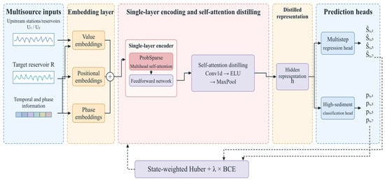
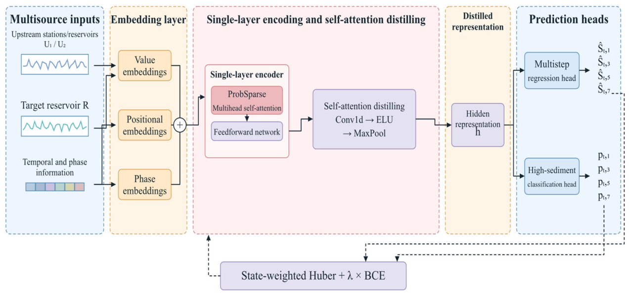
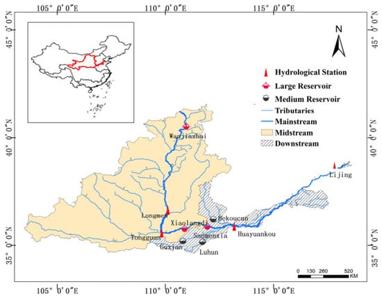
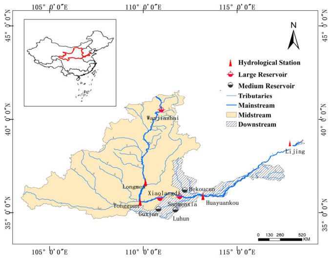
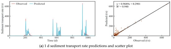
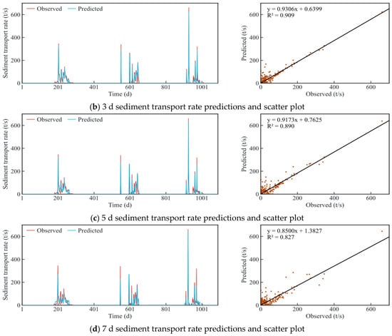
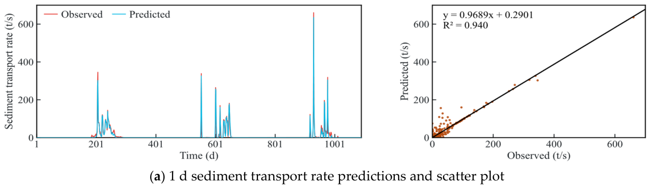
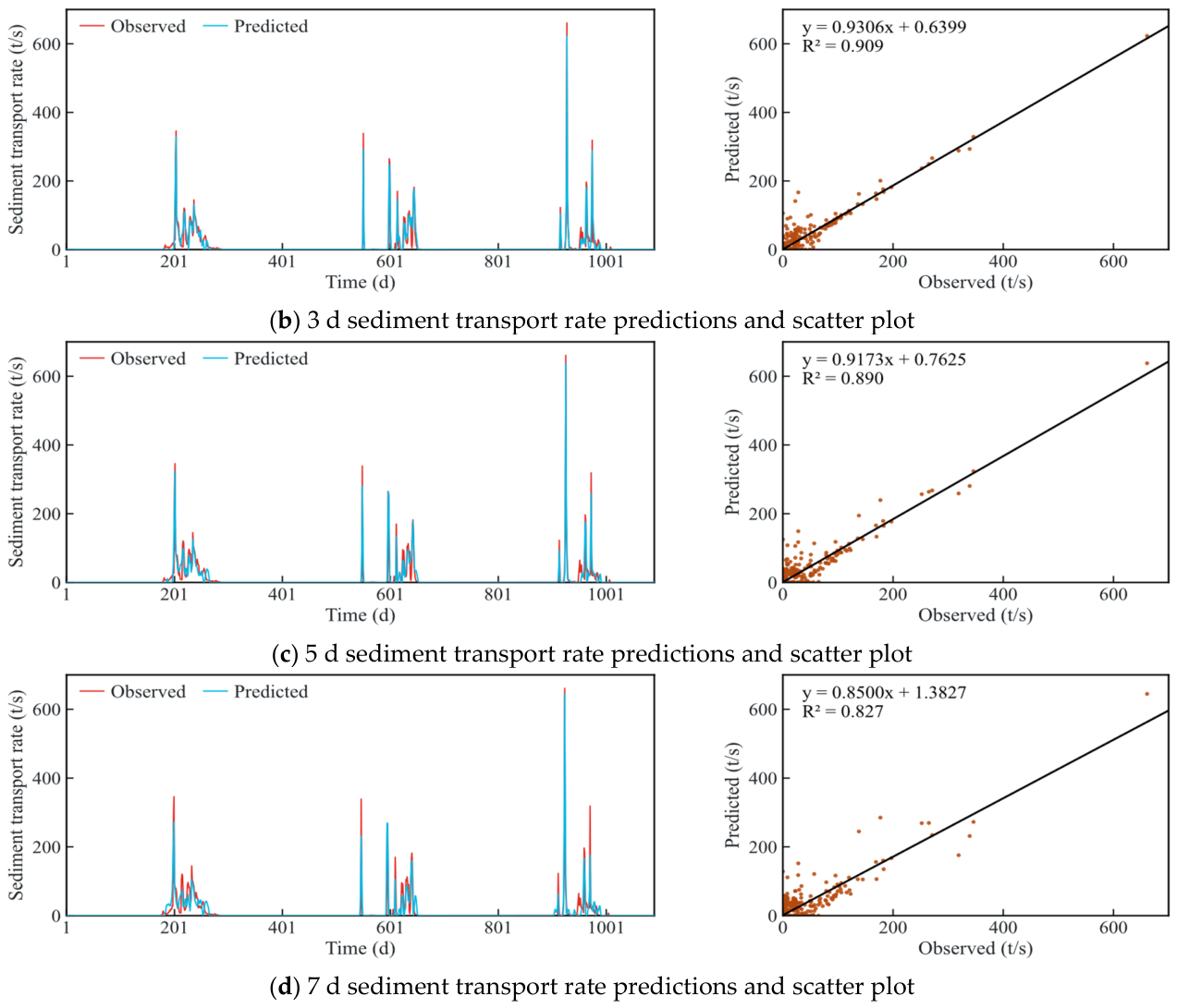
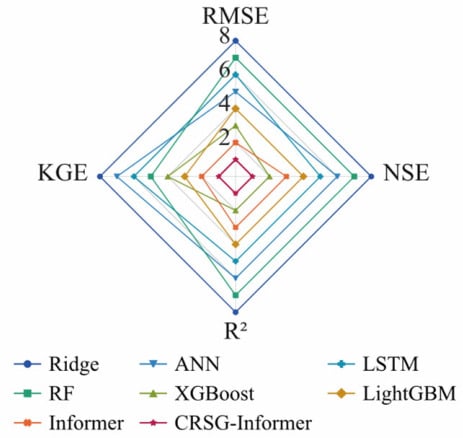
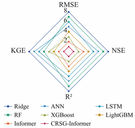
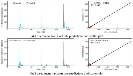
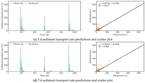
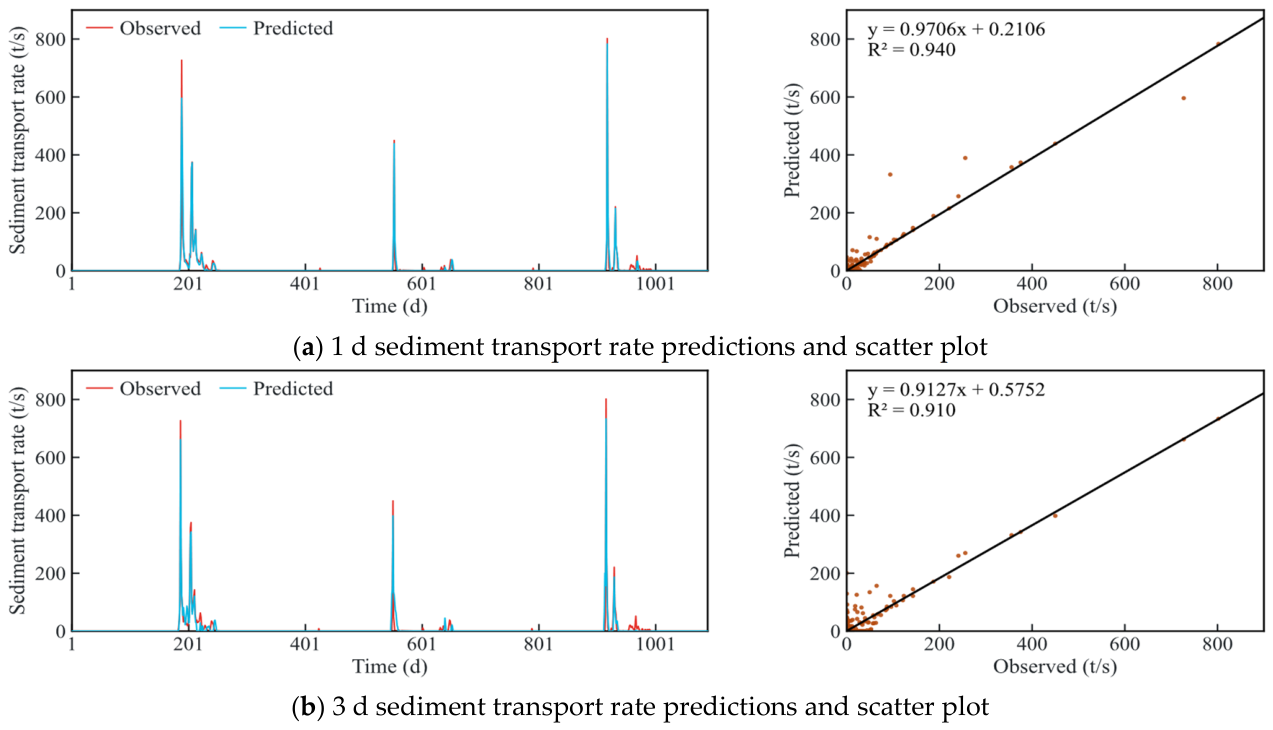
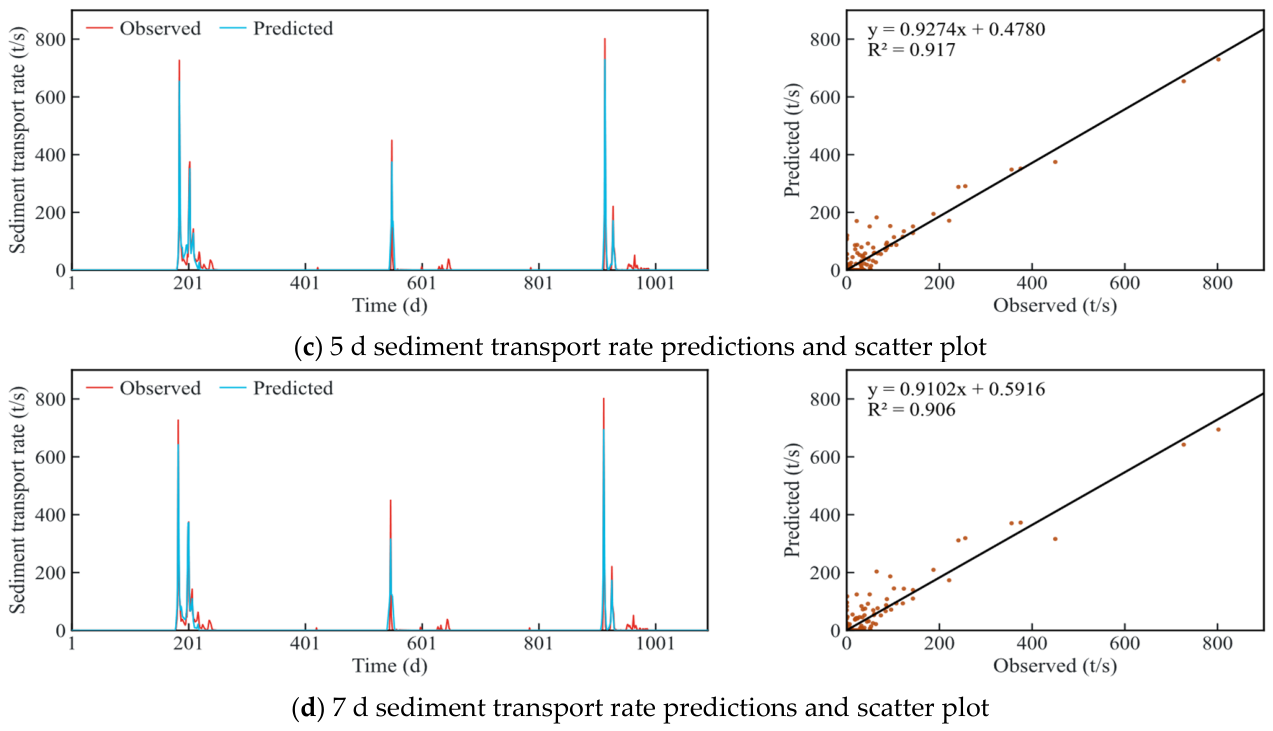
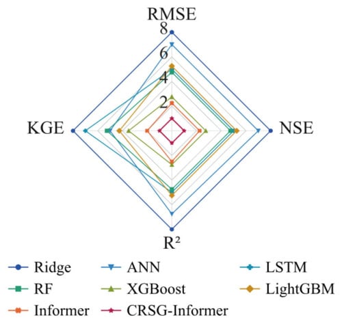
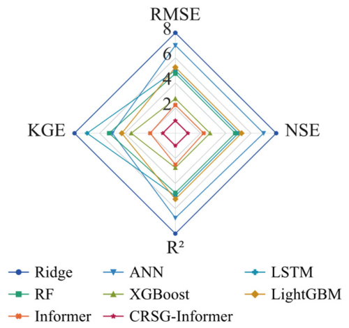
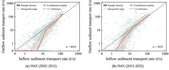
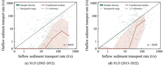
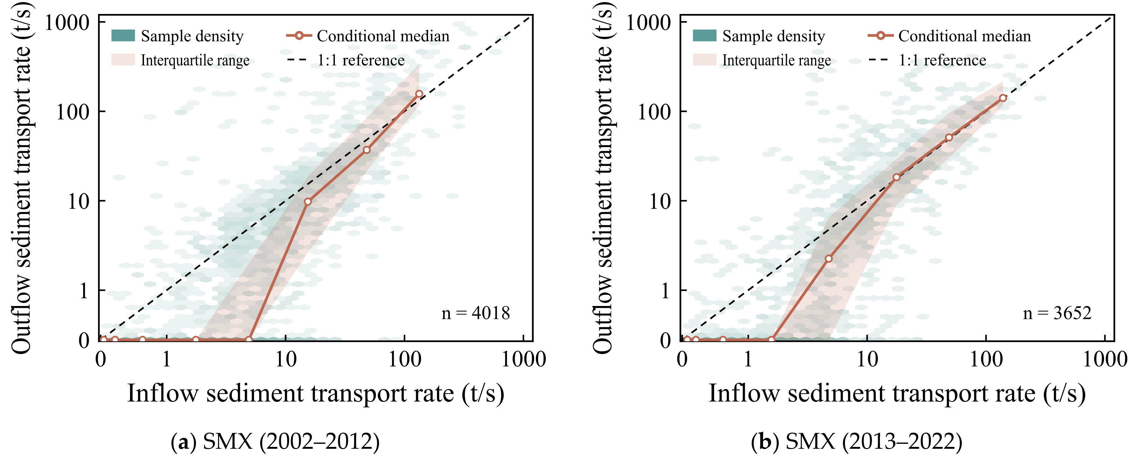
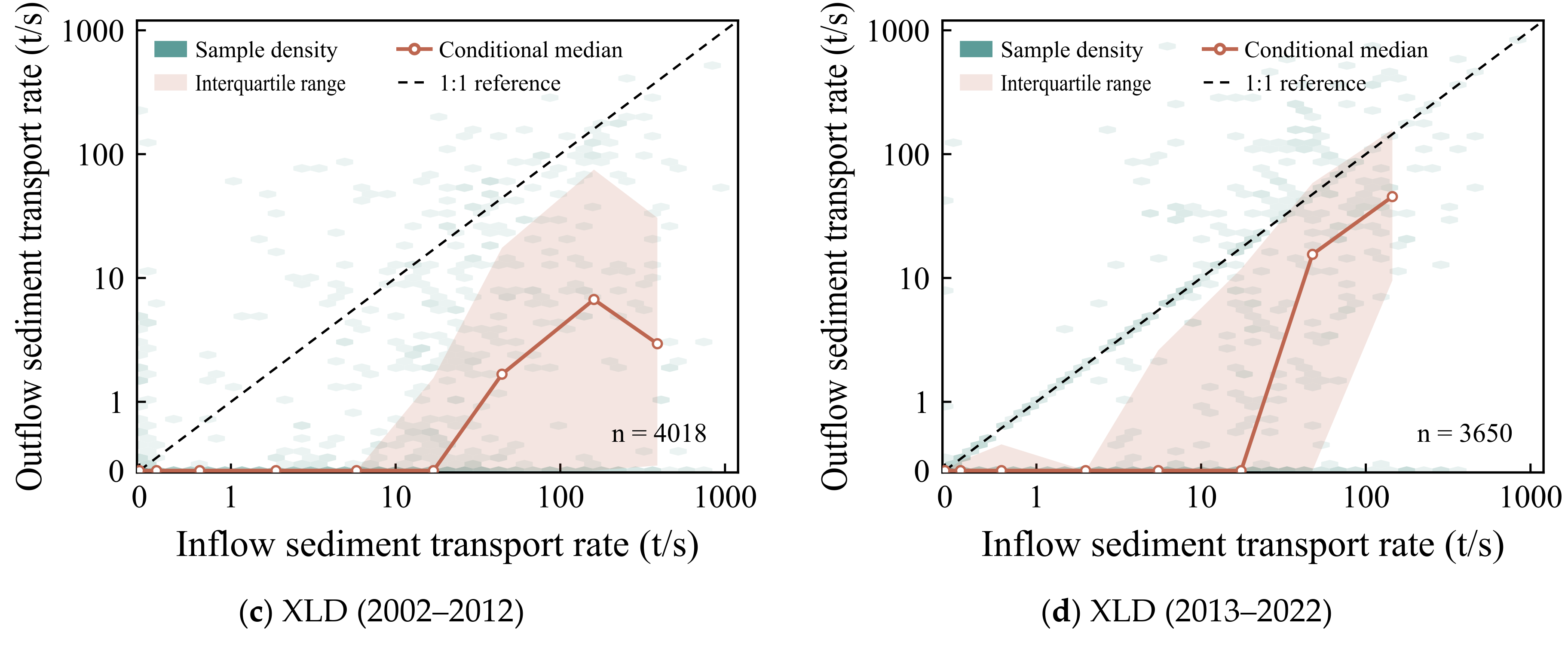
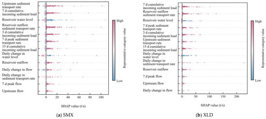
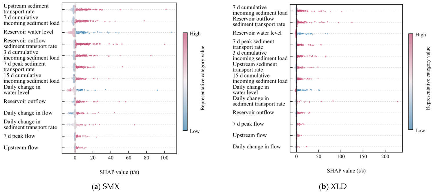
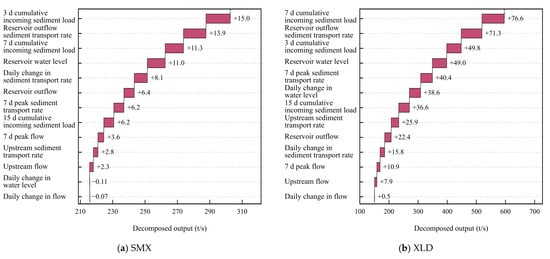
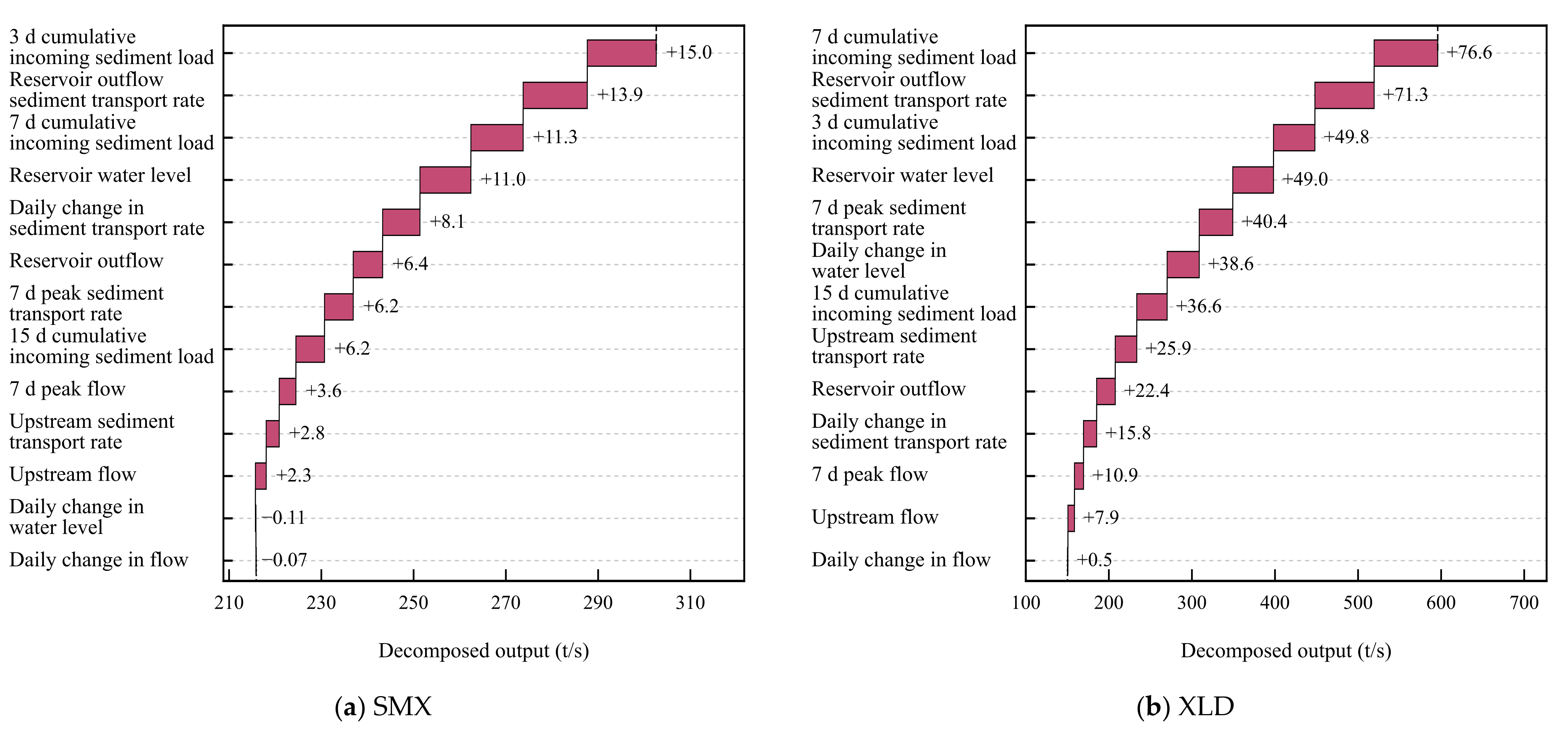
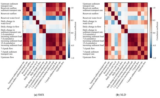
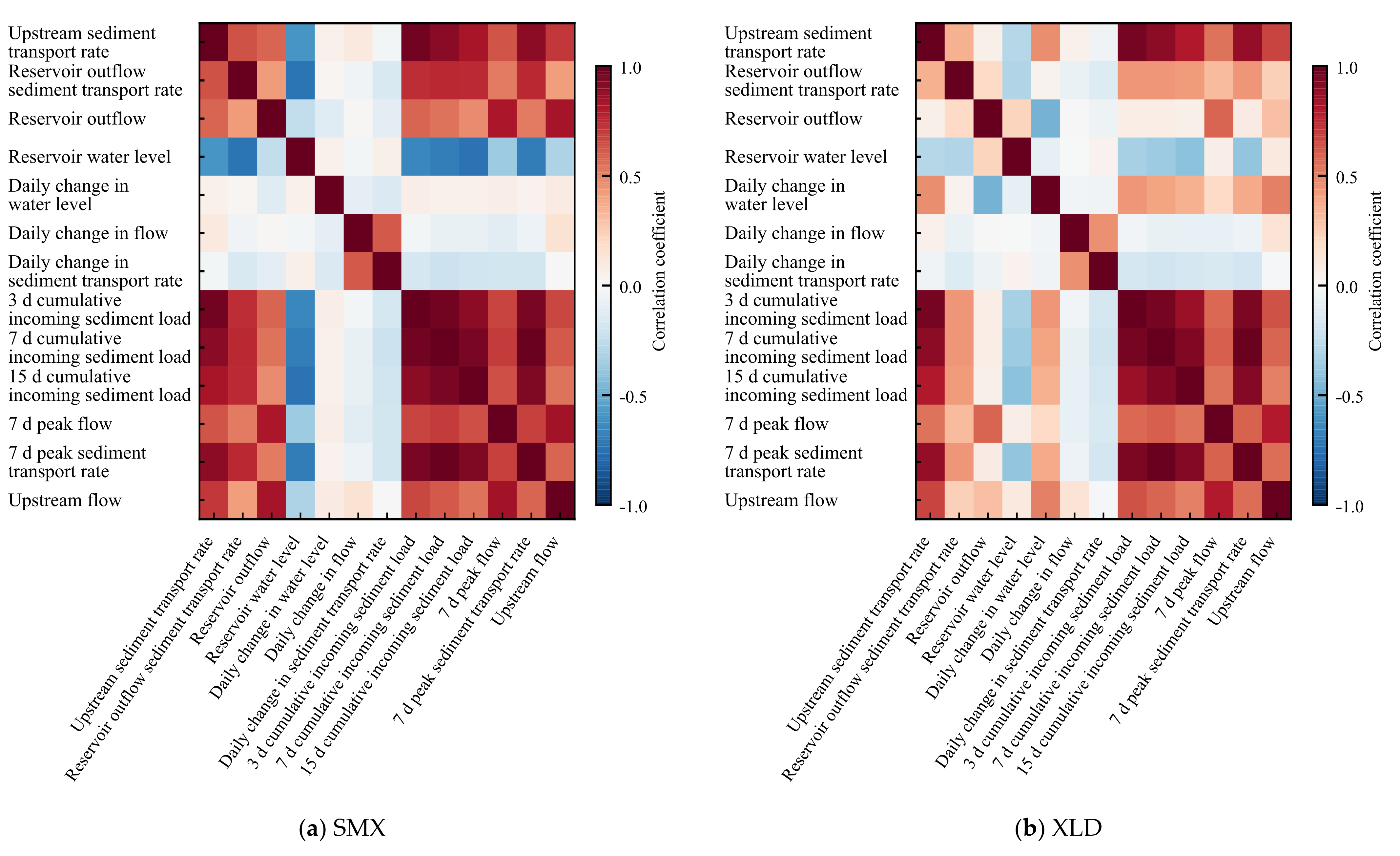
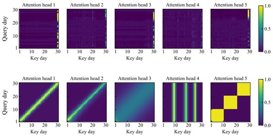
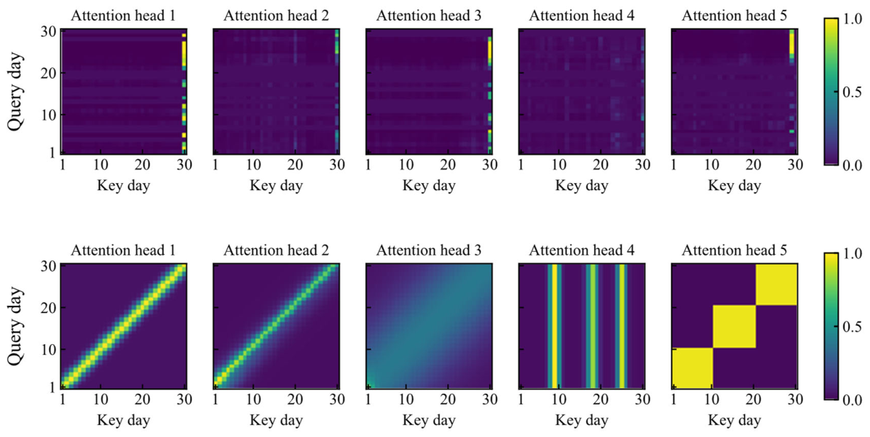
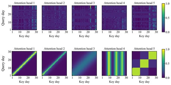
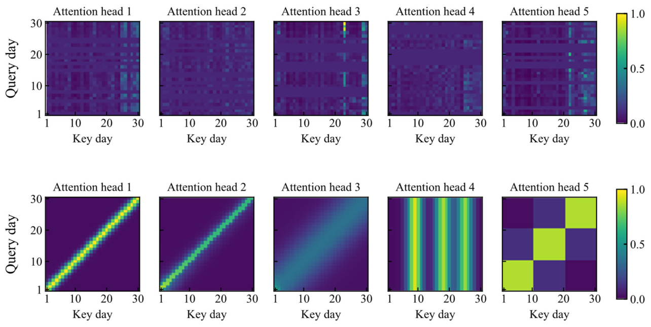
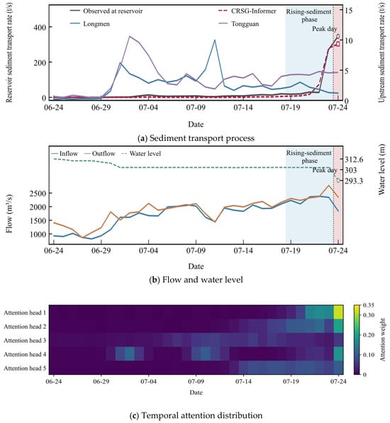
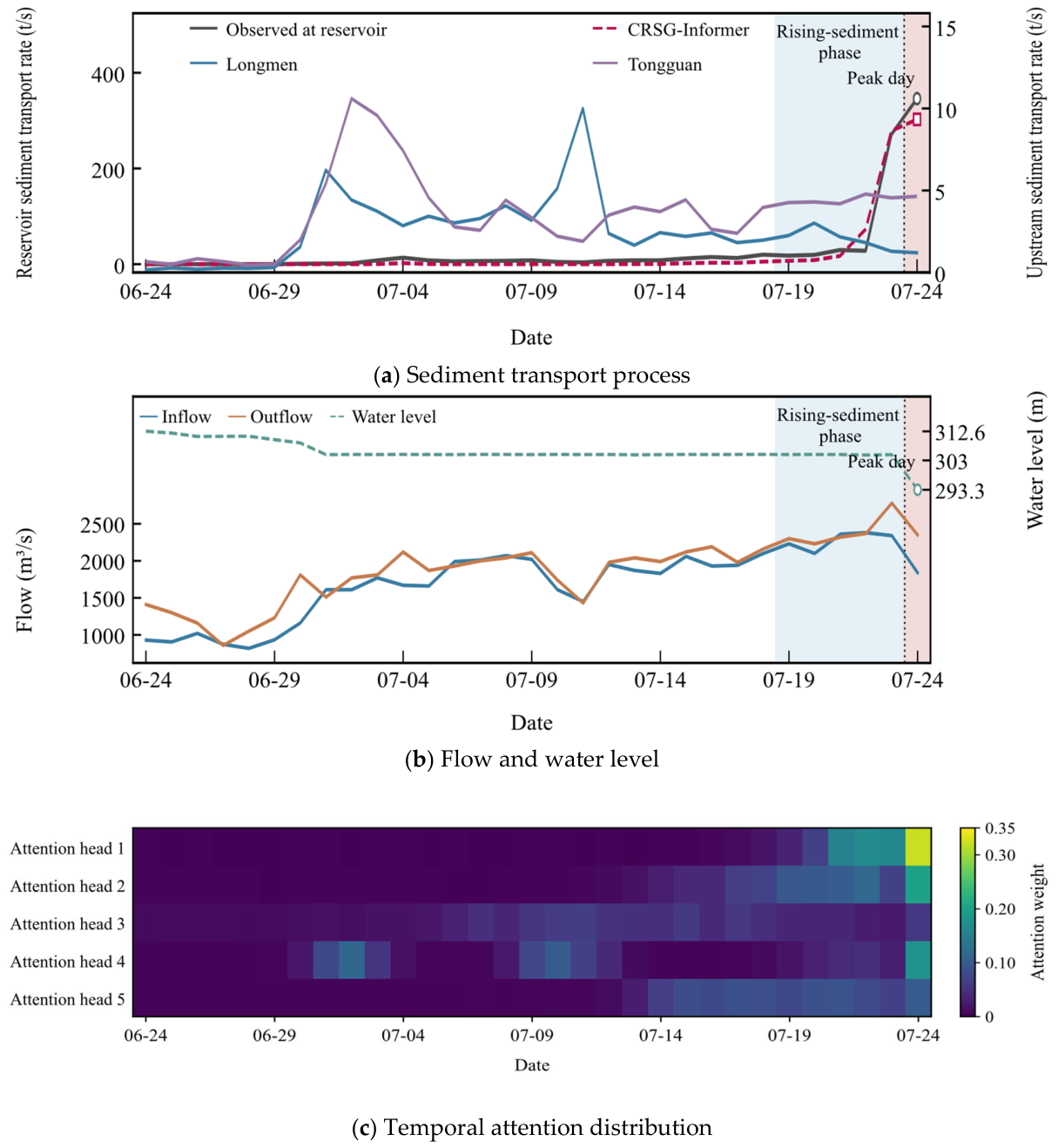
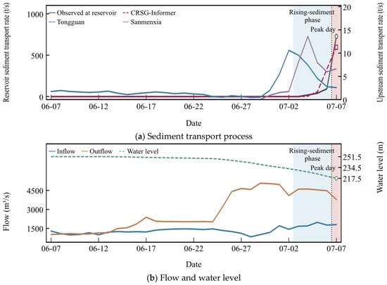
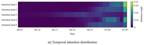
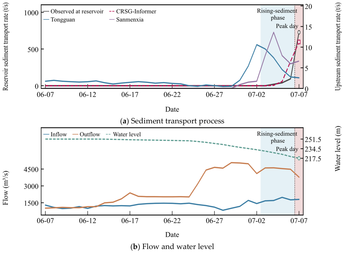
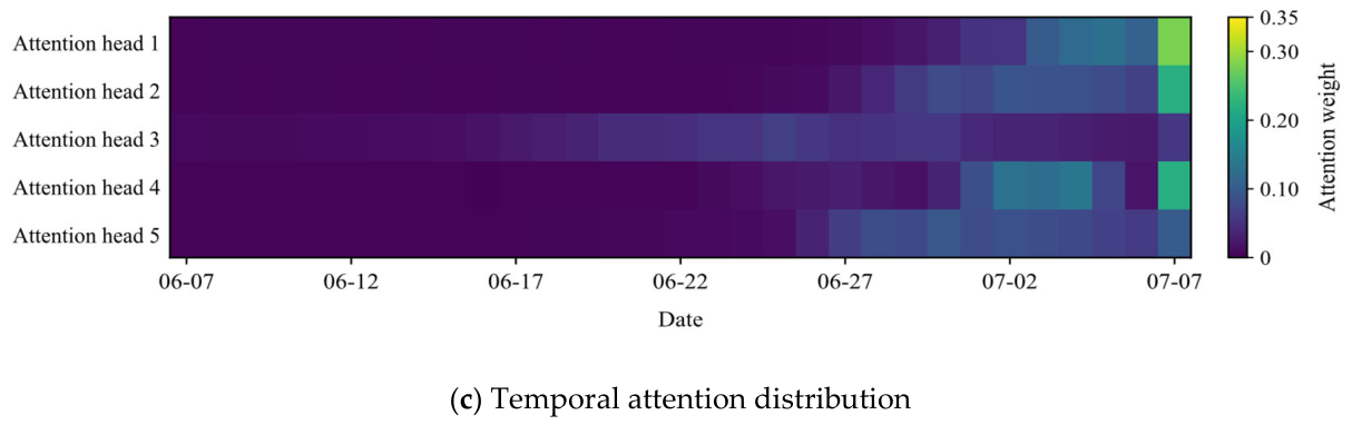
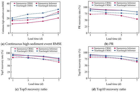
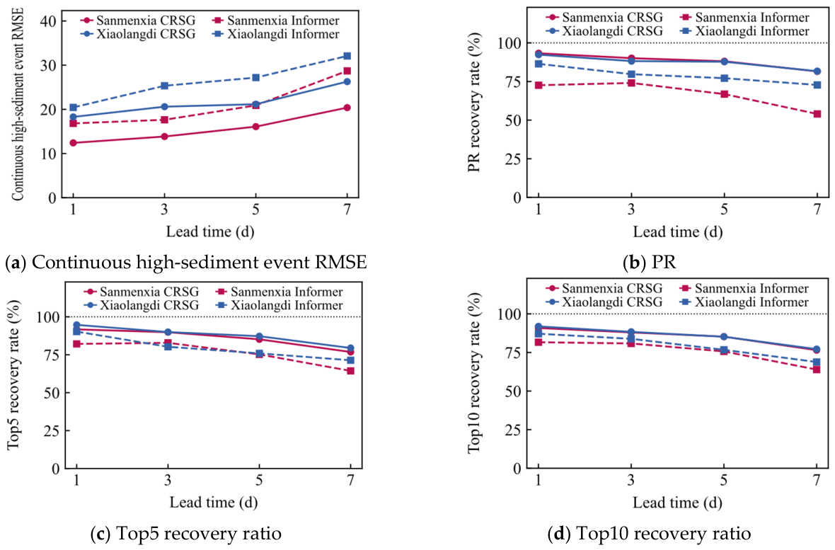
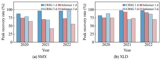
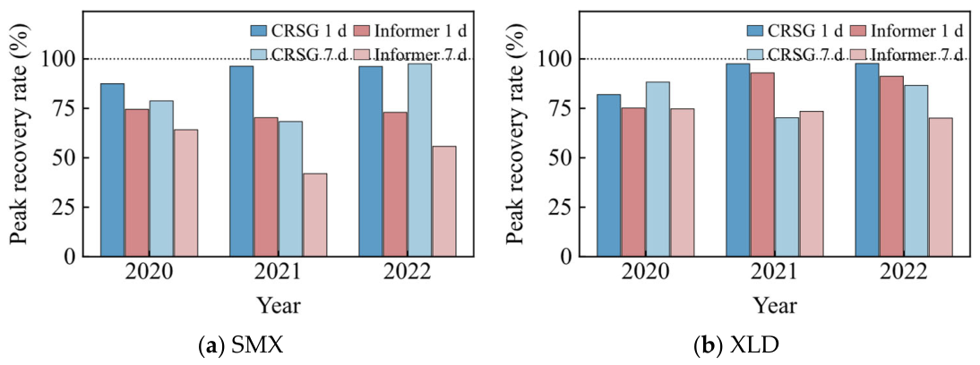
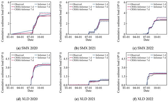
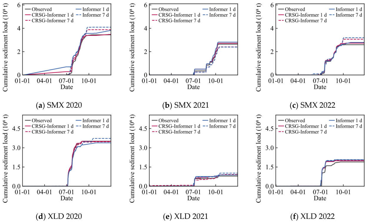
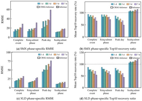
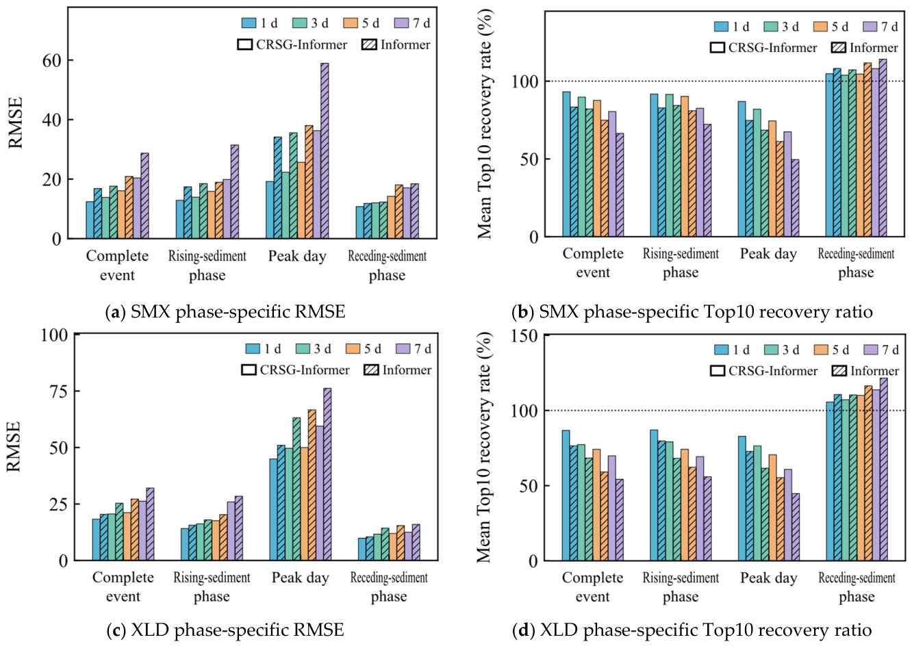
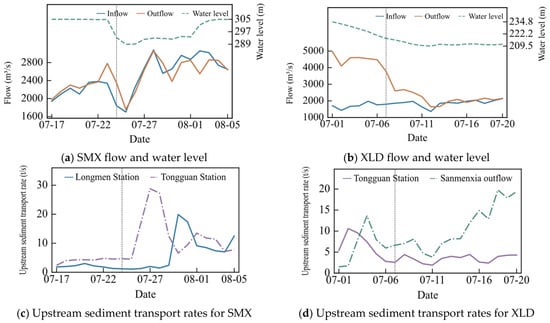
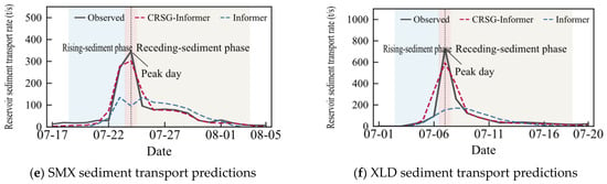
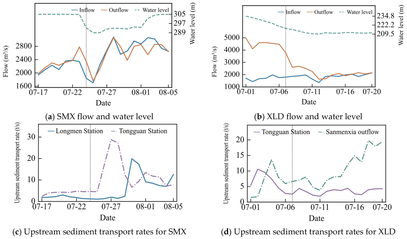
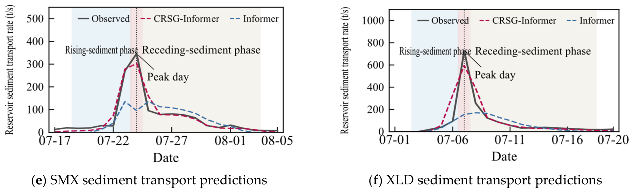
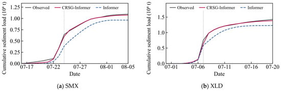
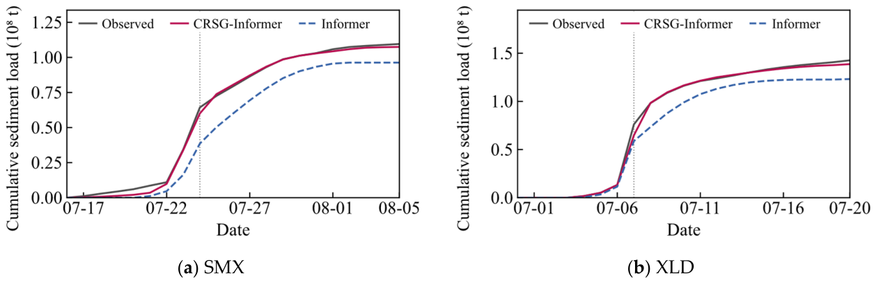
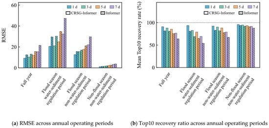
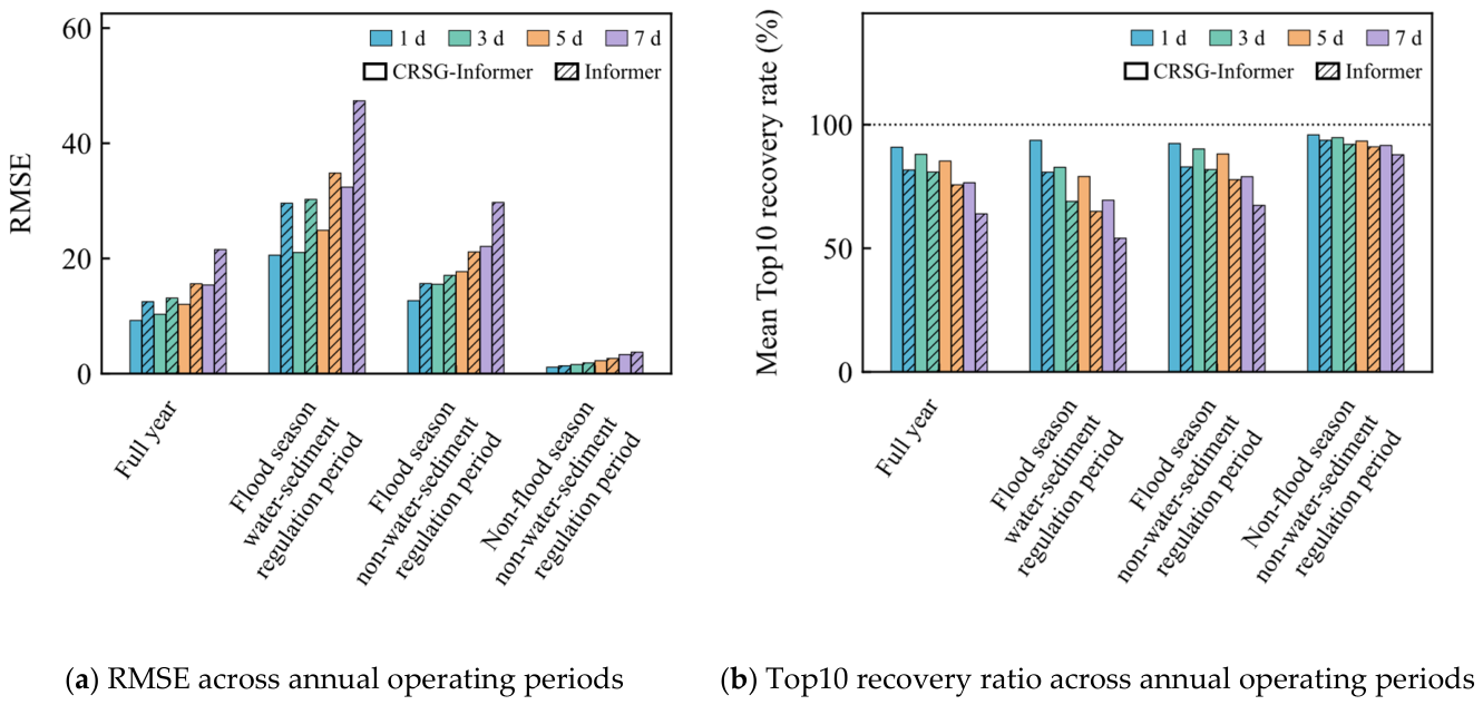
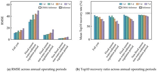
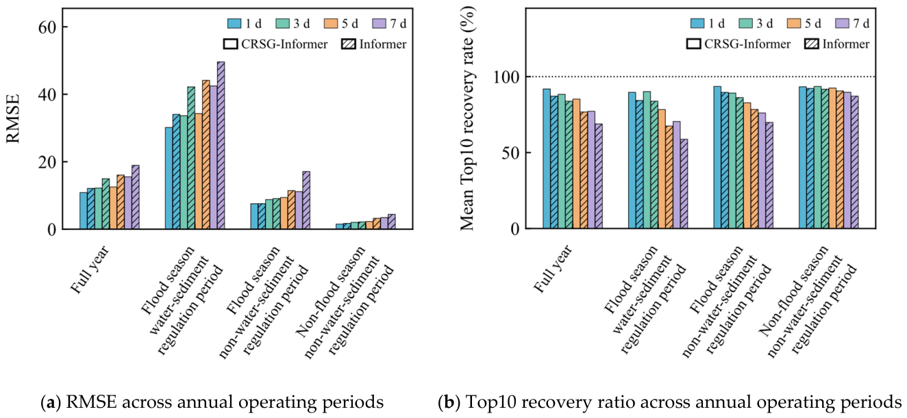

Disclaimer/Publisher’s Note: The statements, opinions and data contained in all publications are solely those of the individual author(s) and contributor(s) and not of MDPI and/or the editor(s). MDPI and/or the editor(s) disclaim responsibility for any injury to people or property resulting from any ideas, methods, instructions or products referred to in the content. |
© 2026 by the authors. Licensee MDPI, Basel, Switzerland. This article is an open access article distributed under the terms and conditions of the Creative Commons Attribution (CC BY) license.