


Abstract
Reliable computer-vision-based monitoring of floating pollutants requires detectors that can identify small objects, accommodate imbalanced pollutant categories, and operate under practical computational constraints. However, conventional aggregate detection metrics may not fully characterize model performance when the class and object-scale compositions of dataset partitions differ substantially. This study presents a distribution-aware evaluation of five representative object detectors—SSD300, RetinaNet, Faster R-CNN, YOLO26n, and RT-DETR-L—for floating-pollutant monitoring on water surfaces. Using a dataset comprising 4274 images, 8 pollutant categories, and 8606 annotated instances, we evaluated overall detection accuracy, class-wise performance, object-scale sensitivity, validation-to-test performance changes, and computational efficiency. The dataset exhibited pronounced class imbalance, with ‘bottle’ accounting for 79.70% of all instances, while small objects constituted 46.40%. The proportion of small objects differed markedly across partitions, accounting for 0.29% of validation instances and 66.19% of test instances. On the test set, RT-DETR-L achieved the highest mAP@0.50 (75.23%) and mAP@0.50:0.95 (45.73%), whereas YOLO26n attained the highest macro-F1 at the predefined confidence threshold (69.64%). RT-DETR-L also achieved the highest small-object AP (32.56%), although performance remained substantially lower for small than for large objects across all detectors. All models showed higher mAP@0.50 but lower mAP@0.50:0.95 on the test set than on the validation set, while their ranking by mAP@0.50:0.95 remained unchanged. Across three random seeds, class-balanced sampling was associated with higher observed mean macro-F1 and rare-class recall, while the observed mean mAP and small-object AP were lower than those of standard training. Given the limited number of runs and the observed between-seed variability, these differences should be interpreted descriptively rather than as statistically established effects. Under the tested configurations, YOLO26n achieved the highest throughput among the detectors evaluated at 640 × 640, whereas SSD300 achieved the highest raw throughput at its lower 300 × 300 input resolution. These findings demonstrate that floating-pollutant detector assessment benefits from jointly considering aggregate accuracy, category-level performance, object scale, partition-level distribution differences, and computational efficiency under the tested configuration.
1. Introduction
Floating pollutants, particularly plastic debris and other solid waste, are persistent environmental concerns in rivers, lakes, reservoirs, estuaries, and coastal waters. Their accumulation can threaten aquatic organisms, degrade habitats, and complicate waterway management. Rivers are also an important pathway through which land-based plastic waste reaches the ocean, highlighting the importance of monitoring pollution before it disperses into marine environments [1,2]. However, conventional field surveys and manual visual observations are often labor-intensive, spatially limited, and difficult to scale for continuous monitoring. Camera-based monitoring combined with computer vision therefore offers a promising approach for improving the efficiency and spatial coverage of floating-pollutant surveillance. Recent studies have investigated deep-learning methods for identifying floating marine plastics [3], detecting and classifying litter from vessel-mounted video [4], and benchmarking floating-waste detection in inland waters [5]. Open datasets and further work on floating-litter detection have also helped establish the feasibility of data-driven monitoring in aquatic environments [6]. Nevertheless, the practical performance of these systems remains dependent on the visual characteristics of the targets, the composition of the training data, and the computational resources available for deployment.
One important challenge is the detection of small objects. Floating pollutants may occupy only a small fraction of an image, particularly when observations are collected from elevated viewpoints or when the camera covers a wide water surface. Small targets provide limited visual information, and their appearance can be obscured by water reflections, wave patterns, background clutter, and changes in illumination. Downsampling in deep neural networks may further weaken the spatial details needed to distinguish small objects from their surroundings. Reviews of deep-learning-based small-object detection have identified feature representation, multiscale learning, contextual information, and training strategies as important factors affecting detection performance [7,8]. Feature Pyramid Networks (FPN) were introduced to strengthen multiscale feature representations through top-down pathways and lateral connections [9], while subsequent research has explored more specialized architectures for small-object detection. In floating-litter monitoring specifically, recent work has investigated dense small-object detection and feature-fusion strategies for water-surface imagery [10]. These developments demonstrate that small-object sensitivity is an important consideration when selecting a detector for aquatic environmental monitoring. However, the performance of a detector on small objects cannot necessarily be inferred from its overall average precision, because aggregate metrics combine targets with substantially different spatial scales.
A second challenge is class imbalance. Class imbalance is an important characteristic of floating-object datasets, but its effect on evaluation metrics depends on how the metrics are aggregated. In this study, mAP is calculated as the unweighted mean of class-specific average precision (AP) values, so each evaluated class contributes equally to the final metric regardless of its number of instances [11]. Consequently, the high prevalence of a category such as bottle does not directly give that category greater weight in mAP. Nevertheless, imbalance remains relevant because class-specific AP estimates are based on different numbers of annotated instances, and rare categories may be more difficult to characterize reliably. Reporting class-wise performance alongside mAP is therefore important for understanding detector behavior across categories.
A third consideration is the diversity of detector architectures and their associated accuracy–efficiency trade-offs. The Single-Shot MultiBox Detector (SSD) introduced a single-stage detection framework that combines predictions from multiple feature maps [12]. Faster R-CNN established a widely used two-stage detection paradigm based on region proposals and subsequent classification and localization [13]. RetinaNet incorporated Focal Loss into a dense one-stage detector [11], while modern real-time detection research has continued to explore architectures that balance inference speed and detection accuracy. The transformer-based Detection Transformer (DETR) formulated object detection as a set-prediction problem [14], and Real-Time Detection Transformer (RT-DETR-L) subsequently addressed computational constraints to enable real-time inference [15]. More recent real-time detector families, including YOLO-based models, provide additional alternatives for practical deployment [16,17]. These architectures differ in their feature extraction, prediction mechanisms, computational requirements, and sensitivity to object characteristics. Therefore, selecting a detector for water-surface monitoring requires more than identifying the model with the highest aggregate accuracy: model size, inference latency, throughput, and the intended monitoring objective also need to be considered.
An additional methodological issue concerns the relationship between dataset composition and reported detection performance. Object detection benchmarks commonly use predefined training, validation, and test partitions, but these partitions may differ in their class frequencies and object-scale distributions. Research on dataset bias and dataset shift has demonstrated that model evaluation can be affected when the evaluation data differ from the data on which a model was developed [18,19]. More recent object-detection benchmarks have explicitly examined performance under natural distribution changes [20] and real-world spatial distribution shifts [21]. Such work provides a broader methodological basis for examining whether the evaluation conditions adequately represent the data encountered in practice. In aquatic monitoring, differences in camera viewpoint, target distance, water-surface appearance, and the relative frequency of pollutant categories may be relevant to future deployment. However, these factors should be measured directly rather than inferred from aggregate performance differences alone. In particular, when acquisition metadata or independent scene-level groupings are unavailable, differences between validation and test partitions should be described as ‘partition-level distribution differences’, rather than being treated as proof of cross-domain generalization or as evidence that a specific distributional factor caused the observed performance changes.
These issues also raise questions about the suitability of relying on a single evaluation metric. The PASCAL Visual Object Classes challenge established widely used conventions for evaluating object detection [22], while the Microsoft Common Objects in Context (COCO) benchmark introduced evaluation across multiple intersection-over-union thresholds and object-area categories [23]. Average precision at a single IoU threshold and averaged precision across multiple thresholds capture different aspects of localization and detection quality. Similarly, precision, recall, and F1-score measured at a specified confidence threshold describe a particular operating point rather than the same property as threshold-integrated average precision. For a monitoring system, a high-recall operating point may be desirable when missing pollutants is costly, whereas high precision may be important when false detections lead to unnecessary inspection or removal operations. Scale-specific average precision and recall can further reveal whether a detector performs consistently across small, medium, and large objects. These complementary metrics are therefore useful for interpreting detector behavior, especially when dataset partitions have substantially different compositions.
Computational efficiency is another essential consideration for continuous monitoring [24,25,26,27]. A model that achieves strong detection accuracy may still be impractical if its latency, memory requirements, or computational cost exceed the capabilities of the intended platform. Conversely, a lightweight detector may provide attractive throughput but miss small or uncommon pollutant categories. Meaningful comparisons consequently require efficiency measurements under a consistent hardware and inference protocol. Parameter count and floating-point operation estimates provide information about model complexity, while measured latency and throughput provide a more direct indication of inference performance under specified experimental conditions. These quantities are related but not interchangeable: measured runtime also depends on input resolution, preprocessing, postprocessing, hardware, and software implementation. A deployment-oriented assessment should therefore report accuracy and efficiency together, while clearly documenting the conditions under which the measurements were obtained.
Against this background, the present study investigates whether conventional aggregate detection metrics provide a sufficiently comprehensive basis for comparing detectors when class and object-scale distributions differ across dataset partitions. Rather than proposing a new architecture, this study evaluates five representative detector configurations—SSD300, RetinaNet, Faster R-CNN, YOLO26n, and RT-DETR-L—using a common floating-pollutant dataset and a consistent experimental protocol. The analysis integrates overall detection accuracy, class-wise performance, object-scale sensitivity, validation-to-test performance changes, and computational efficiency. In addition, targeted training interventions are examined to assess whether class-balanced and scale-aware strategies improve selected monitoring outcomes.
The contributions of this study are threefold. First, we provide a comparative evaluation of five representative object detectors for water-surface floating-object detection, considering aggregate accuracy alongside class-specific, object-scale-specific, and operating-point performance. Second, we characterize the differences in class and object-scale composition between the released validation and test partitions and examine how the observed performance differences depend on the evaluation metric. This analysis is explicitly limited to partition-level differences and does not establish generalization across independently acquired domains. Third, we conduct a controlled training-sampling intervention on YOLO26n using class-balanced and scale-aware strategies, reporting their effects across complementary metrics, including cases in which the interventions do not improve aggregate or small-object AP. Together, these analyses provide a framework for interpreting detector performance beyond a single aggregate metric under the specific dataset and experimental conditions examined here.
The study addresses three objectives: (1) to characterize class imbalance and object-scale composition in the dataset and quantify detector performance across pollutant categories and object sizes; (2) to compare representative detection architectures in terms of aggregate accuracy, operating-point performance, and computational efficiency under the tested configuration; and (3) to examine how validation-to-test performance differences depend on the evaluation metric when the two partitions have different class and object-scale compositions. By combining these perspectives, the study aims to provide a more transparent and application-oriented framework for evaluating deep-learning detectors for camera-based aquatic environmental monitoring. The analysis is intended to support detector selection under the tested dataset and experimental conditions, rather than to establish generalization to unobserved geographical, sensor, or acquisition domains.
2. Materials and Methods
This study establishes a distribution-aware evaluation framework to systematically assess deep learning detectors for floating-pollutant monitoring on water surfaces. The framework is designed around three practical characteristics of water-surface pollutant detection: the prevalence of small objects, severe class imbalance, and the computational constraints associated with real-time deployment. Rather than evaluating detector performance using overall mean average precision (mAP) alone, the proposed framework decomposes detection capability into four complementary dimensions: overall detection accuracy, object-scale sensitivity, category-level robustness, and computational efficiency.
The overall workflow consists of five stages. First, the dataset is statistically characterized in terms of image distribution, class frequency, bounding-box size, and the distribution of these properties across the training, validation, and test partitions. Second, representative deep learning detectors with different architectural paradigms are trained under a unified experimental protocol. Third, detector performance is evaluated using conventional detection metrics together with object-scale-specific and class-wise metrics. Fourth, validation-to-test performance changes are quantified to determine whether detector performance is sensitive to differences in class and object-scale distributions between dataset partitions. Finally, a balanced-training intervention is introduced to examine whether the performance limitations identified by the distribution-aware analysis can be alleviated through class- and scale-aware training strategies.
2.1. Dataset and Distribution Characterization
This study used a publicly available floating-pollutant object detection dataset as the sole image source for all experiments. The dataset contains 4274 JPEG images with a spatial resolution of 640 × 640 pixels and 8606 annotated bounding-box instances across eight annotated floating-object categories: ball, bottle, branch, grass, leaf, milk-box, plastic-bag, and plastic-garbage. The 8606 annotated instances were distributed as 5893 training, 341 validation, and 2372 test instances. The dataset was obtained from Roboflow Universe (workspace: objectdetection-jdedj; project: -9uy6g; export version: v3) and is released under the CC BY 4.0 license. Images were exported in YOLO object-detection format, where each object is represented by a class identifier and normalized bounding-box coordinates. The export process included automatic orientation correction, removal of EXIF orientation information, and stretching of images to 640 × 640 pixels; no image augmentation was applied during dataset export. The dataset includes both anthropogenic floating litter, such as bottles and plastic bags, and naturally occurring floating materials, such as branches, grass, and leaves. Because the annotations define visual object categories rather than independently verified environmental pollution status, we use “floating objects” when referring to the full detection task and retain the original category labels when reporting class-specific results.
The original dataset was divided into 3011 training images, 231 validation images, and 1032 test images, corresponding to 70.45%, 5.40%, and 24.15% of the total images, respectively. The eight categories exhibit substantial class imbalance. Bottle is the dominant category, accounting for 6859 instances (79.70% of all annotations), whereas ball is the least frequent category, with only 46 instances (0.53%). In addition, only four ball instances occur in the validation set and seven in the test set, indicating that class-specific performance for this category may have relatively high statistical uncertainty.
Before model training, the dataset was quantitatively characterized in terms of class composition and object-scale distribution. For each class c, the total number of annotated instances was calculated as:
where N denotes the number of images and ni,c is the number of instances of class c in image i. The proportion of each class was calculated as:
where C = 8 is the number of object categories. To quantify the severity of class imbalance, an imbalance ratio was defined as:
For each ground-truth bounding box, the box area was calculated as:
where w and h denote the bounding-box width and height in pixels. The relative box area was additionally calculated as:
where W = H = 640 represents the image dimensions. Ground-truth objects were categorized according to their bounding-box area in the original 640 × 640 annotation space:
Abox = w × h,
Small: Abox < 322,
Medium: 322 ≤ Abox < 962,
Large: Abox ≥ 962.
These thresholds were applied to the ground-truth annotations before model evaluation and were not affected by the internal input resolution of an individual detector. Using these definitions, the dataset contains 3993 small objects (46.40%), 3152 medium objects (36.63%), and 1461 large objects (16.98%). Furthermore, 69.03% of all annotated objects occupy less than 1% of the full image area. These characteristics indicate that the dataset simultaneously exhibits strong class imbalance and a substantial small-object component.
The train, validation, and test partitions were further compared to identify potential distribution differences. For a distribution variable d, including class identity or object-scale category, the proportion in partition p was calculated as:
where Np(d) denotes the number of instances associated with distribution component d in partition p. The comparison revealed pronounced differences in object-scale composition. Small objects account for 41.10% of annotated objects in the training set, only 0.29% in the validation set, and 66.19% in the test set. The class distribution also differs substantially across partitions. For example, bottle represents 76.70% of training annotations and 91.91% of test annotations, whereas its proportion in the validation set is 46.63%.
These differences were treated as partition-level class and object-scale distribution shifts. They were not interpreted as evidence of cross-domain generalization because information regarding acquisition environment, geographical location, imaging device, or capture conditions was unavailable. The purpose of this analysis was instead to determine whether conventional validation-based detector evaluation remains reliable when the test partition has substantially different class and scale composition. All experiments used the original train/validation/test partition without incorporating external image datasets. The training set was used exclusively for model optimization, the validation set was used for model selection and threshold determination where required, and the test set was reserved for final performance evaluation and distribution-shift analysis. No test-set samples were used for model selection, hyperparameter tuning, or training-strategy selection.
Prior data-quality inspection found no missing image-label pairs, no apparent bounding-box format or coordinate-value anomalies, and no exact duplicate images across the three partitions based on both file-content and decoded-pixel comparisons. One training image was associated with an empty annotation file despite a visually identifiable floating object and was therefore flagged for manual review before formal model training. Because systematic linkage analysis of near-duplicate scenes was not available, this study does not claim complete scene-level independence across the three partitions. Likewise, the available dataset documentation does not provide sufficient information about original acquisition locations, imaging devices, acquisition dates, or detailed annotation procedures. Accordingly, the distribution differences analyzed in this study are defined strictly at the dataset-partition level rather than interpreted as geographical, sensor-level, or environmental domain shifts.
The training, validation, and test partitions were adopted directly from the original Roboflow dataset release; the authors did not independently repartition the images. However, the released validation partition contains only one small object under the scale definition used in this study. Consequently, it is not sufficiently representative for reliable small-object checkpoint selection, threshold tuning for scale-sensitive applications, or rigorous evaluation of scale-aware training strategies. The validation-to-test comparison is therefore interpreted as a descriptive analysis of performance differences between the released partitions, rather than evidence of generalization across independently acquired domains. This limitation should be considered when interpreting the scale-specific results and the training interventions.
2.2. Detector Selection and Training Protocol
Five representative object-detection architectures were selected to cover distinct detector paradigms: (1) SSD300, representing a classical one-stage convolutional detector; (2) RetinaNet, representing a one-stage detector incorporating focal loss for addressing foreground–background imbalance; (3) Faster R-CNN with ResNet-50-FPN, representing a two-stage convolutional detector; (4) YOLO26n, representing a lightweight modern real-time YOLO-family detector; (5) RT-DETR-L, representing a real-time transformer-based detection architecture.
The purpose of this selection was not to construct an exhaustive benchmark of all available detectors, but to provide architectural diversity while maintaining a manageable and interpretable experimental design. The selected models therefore represent classical one-stage detection, imbalance-aware one-stage detection, two-stage region-based detection, lightweight real-time convolutional detection, and transformer-based real-time detection.
All experiments were conducted using Google Colab (Google LLC, Mountain View, CA, USA) with an NVIDIA A100-SXM4-40GB GPU (NVIDIA Corporation, Santa Clara, CA, USA). The software environment included Python 3.13.15 (Python Software Foundation, Beaverton, OR, USA), PyTorch 2.11.0+cu130, torchvision 0.26.0+cu130, Ultralytics 8.4.173, and pycocotools 2.0.11. All detectors were trained using the training partition and evaluated independently on the validation and test partitions. The training protocol, optimization settings, data augmentation policy, input resolution, batch size, learning rate, optimizer, weight decay, learning-rate schedule, warm-up strategy, random seed, and checkpoint-selection criterion were fixed before final test evaluation and are reported in Table 1.
Table 1.
Configurations and training settings of the evaluated object detectors.
For each detector, the best checkpoint was selected according to performance on the validation set. The primary checkpoint-selection criterion was mAP50:95, while the test set was not used for checkpoint selection or hyperparameter optimization. This protocol prevents information from the test partition from influencing the trained model or the reported final performance. Model-specific input dimensions were retained where required by the selected detector architecture. In particular, SSD300 was evaluated using its designated 300 × 300 input resolution, whereas the input resolution adopted for the remaining detectors is recorded explicitly in Table 1.
To ensure comparability, all models were evaluated using the same ground-truth annotations and the same class definitions. Object-scale categories were assigned from the original 640 × 640 ground-truth bounding boxes rather than from model-specific resized images. For metrics that require a confidence threshold, the threshold was determined using the validation set and subsequently fixed for test evaluation. No confidence threshold was tuned on the test set. In contrast, AP and mAP were calculated from the confidence-ranked predictions and therefore did not depend on selecting a single operating threshold. Each model configuration was evaluated using three fixed random seeds (17, 42, and 2026). The reported results are presented as the arithmetic mean and sample standard deviation across the three runs.
2.3. Detection Performance Metrics
Detector performance was evaluated using precision, recall, F1-score, AP, and mAP. Precision and recall were calculated as:
where TP, FP, and FN denote true positives, false positives, and false negatives, respectively. The F1-score was calculated as:
For class-balanced evaluation, the macro-averaged F1-score was calculated as:
where F1,c represents the F1-score of class c. Macro-F1 assigns equal importance to all categories and is therefore particularly informative for the highly imbalanced pollutant dataset.
Average Precision at an IoU threshold of 0.50 was calculated for each class, and the mean across all eight classes was reported as:
To evaluate localization quality over a wider range of IoU thresholds, the primary strict detection metric was defined as:
Thus, mAP50:95 represents the mean mAP over IoU thresholds of 0.50, 0.55, 0.60, …, 0.95. IoU was defined as:
where Aintersection is the area of overlap between a predicted and ground-truth bounding box and Aunion is their union area.
Because a substantial proportion of the dataset consists of small objects, detection performance was explicitly evaluated as a function of object scale. For each scale category s∈{S, M, L}, AP was calculated over the IoU thresholds from 0.50 to 0.95:
The resulting APS, APM, and APL quantify detection performance for small, medium, and large ground-truth objects, respectively. Scale-specific recall was calculated as:
The scale category was always assigned according to the area of the corresponding ground-truth bounding box in the original 640 × 640 image. The size of a predicted box was not used to determine the ground-truth scale category. This analysis allows the detectors to be compared not only according to overall accuracy but also according to their ability to detect small targets, which is particularly relevant to water-surface floating-pollutant monitoring.
2.4. Class-Imbalance and Distribution-Shift Evaluation
The relationship between class frequency and detector performance was examined to determine whether common categories are systematically easier to detect than rare categories. For each class c, its training-set frequency Nc was compared with class-specific AP and recall. Spearman’s rank correlation coefficient was calculated as:
and
ρAP = Spearman(Nc,APc),
ρRecall = Spearman(Nc,Recallc).
A positive correlation indicates that more frequently represented categories tend to achieve higher detection performance, whereas a weak or negative correlation suggests that category frequency alone does not explain class-wise performance.
In addition to class-specific AP and recall, Macro-F1 was used as a class-balanced summary metric. Rare-class recall was calculated by first defining rare categories according to their training-set annotation frequency. Categories representing less than 3% of the training annotations were considered rare categories, and their mean class-specific recall was calculated as:
where Crare denotes the predefined set of rare categories. The 3% threshold was fixed before the intervention experiments and was not modified according to the resulting detector performance. This analysis was used to determine whether overall mAP could conceal systematic weaknesses in low-frequency pollutant categories.
The central distribution-aware analysis compared detector performance between the validation and test partitions. For any performance metric M, the absolute change between the two partitions was defined as:
ΔM = MTest − MVal.
For overall detection performance,
ΔmAP = mAPTest − mAPVal.
Scale-specific changes were calculated as:
and
ΔAPS = APS,Test − APS,Val,
ΔAPM = APM,Test − APM,Val,
ΔAPL = APL,Test − APL,Val.
To express the magnitude of performance degradation relative to validation performance, the relative performance drop was calculated as:
For mAP, this becomes:
A complementary shift-retention ratio was calculated as:
and, for mAP specifically,
Values of Rshift closer to 1 indicate stronger retention of validation performance on the test partition, whereas lower values indicate a larger relative performance loss.
The stability of model rankings was additionally assessed as:
where j denotes a detector. A value of zero indicates unchanged ranking, a positive value indicates that the model moved to a lower rank on the test set, and a negative value indicates an improvement in rank.
ΔRankj = RankTest(j) − RankVal(j),
The distribution-shift analysis was conducted without retraining the detectors. The same trained checkpoints and evaluation conventions were applied independently to the validation and test partitions.
2.5. Computational Efficiency and Training Intervention
In addition to detection accuracy, the computational and deployment characteristics of all five detectors were evaluated. The evaluated indicators included parameter count, theoretical computational complexity, serialized model size, inference latency, frames per second (FPS), and, where measurement conditions were consistent, peak GPU memory consumption.
The number of trainable parameters was reported in millions (M). Theoretical computational complexity was reported as GFLOPs, calculated at the actual input resolution used by each detector. Inference latency was measured using batch size 1 to approximate single-frame or sequential-image monitoring. After an initial warm-up period, multiple consecutive inference iterations were timed under identical hardware, software, and numerical-precision conditions. Disk I/O and dataset-loading time were excluded. Model forward inference and the necessary model-specific post-processing were included in the reported inference latency.
The mean inference time was calculated as:
where Ti denotes the measured inference time of the i-th image. For batch size 1, inference throughput was calculated as
where Tinf is expressed in milliseconds per image. Model size was measured from the serialized weights-only checkpoint rather than estimated from parameter count. Peak GPU memory, when reported, was measured under the same batch size, input resolution, numerical precision, and hardware conditions used for latency benchmarking.
All computational-efficiency measurements were performed under a common hardware and software environment, which is recorded together with the corresponding model configuration. These measurements were subsequently combined with the accuracy results to examine the accuracy–efficiency trade-off among the evaluated detectors.
Following the distribution and performance analyses, a targeted training intervention was conducted to investigate whether the identified class and object-scale imbalance could be mitigated through training-strategy modification. Rather than retraining all detector architectures under every possible configuration, the intervention was conducted using the detector selected from the preceding benchmark as the representative model. The selected detector was determined from the preceding validation-based analysis by jointly considering detection accuracy, small-object sensitivity, distribution-shift robustness, and computational efficiency. YOLO26n was selected for the intervention experiments as a lightweight representative detector. The intervention study was designed to examine the effects of the specified sampling strategies on this model, rather than to establish their general applicability across detector architectures.
Four training strategies were compared: (1) Standard training, using the baseline training procedure; (2) class-balanced training, designed to reduce the influence of the severe class-frequency imbalance; (3) scale-aware training, designed to increase the model’s sensitivity to the small-object component of the dataset; (4) combined training, incorporating both class-balanced and scale-aware strategies. Class-balanced training was implemented by modifying image-sampling probabilities based on the class annotations in the training set. Images were sampled with replacement according to normalized image-level weights. This intervention did not modify the classification or localization loss functions. The image-weight calculation and sampling procedure are provided in Appendix A.1.
For class-balanced training, category weights were defined as:
where N is the total number of training instances, C is the number of classes, and Nc is the number of training instances belonging to class c. The resulting weights were incorporated into the classification-loss calculation according to the implementation of the selected detector.
The scale-aware strategy was designed to explicitly increase the contribution of small-object detection during training. The specific implementation was fixed before the final test evaluation and documented together with the training configuration. The combined strategy applied both the predefined class-balancing and scale-aware mechanisms.
The four strategies were first compared on the validation set. Validation performance was used to select the final training strategy, thereby preventing the test set from being used for intervention selection. The selected strategy was then evaluated once on the test set using the same evaluation protocol as the baseline detector.
The intervention was evaluated using mAP50, mAP50:95, APS, APM, APL, F1,macro, and Recallrare. These metrics were selected to simultaneously characterize overall detection accuracy, localization quality, small-object sensitivity, medium- and large-object performance, class-balanced performance, and rare-category detection capability. Improvements or degradations relative to standard training were interpreted in conjunction with the distribution-shift analysis rather than solely according to overall mAP. In particular, an intervention was considered potentially beneficial even when overall mAP changed only marginally if it produced a meaningful improvement in small-object detection, Macro-F1, or rare-class recall without causing an unacceptable loss in overall detection performance.
The scale-aware intervention modified the image-sampling probabilities rather than the classification or localization losses. Sampling weights were calculated exclusively from the training annotations. Images containing at least one ground-truth bounding box with an area below 1024 pixels2 in the original 640 × 640 annotation space received an increased sampling weight. During each epoch, 3010 image samples were drawn with replacement according to the normalized sampling probabilities, while the training budget remained 95 optimizer updates per epoch. Consequently, an image could be sampled multiple times, whereas other images might not be selected in a particular epoch.
3. Results
3.1. Dataset Characteristics and Distribution Differences
The dataset comprised 4274 images and 8606 annotated object instances across eight floating-pollutant categories (Table 2 and Table 3). The original partition contained 3011 training images, 231 validation images, and 1032 test images. One training image with an empty annotation file was excluded from model training following data-quality inspection, resulting in 3010 training images being used for optimization. The annotated instance count remained unchanged at 5893 for the training partition. The validation and test partitions contained 341 and 2372 annotated instances, respectively.
Table 2.
Dataset-level statistics.
Table 3.
Class distribution.
The test set contains 1570 small objects under the mutually exclusive size grouping used for dataset characterization in Table 2. The COCO evaluator assigns objects to scale-specific evaluation ranges according to its area-range conventions, which may produce a count of 1571 for the small-object evaluation subset. These counts therefore refer to different grouping procedures and should not be treated as directly interchangeable.
The class distribution was markedly imbalanced. ‘Bottle’ accounted for 6859 instances, representing 79.70% of all annotations, whereas ‘ball’ accounted for only 46 instances (0.53%). The remaining categories were substantially less frequent than ‘bottle’: ‘branch’ contributed 4.88% of all instances, followed by ‘plastic-bag’ (4.55%), ‘leaf’ and ‘milk-box’ (2.96% each), ‘plastic-garbage’ (2.31%), and ‘grass’ (2.09%). The resulting difference between the most and least frequent categories indicates that aggregate detection metrics could be disproportionately influenced by performance on the dominant ‘bottle’ category.
The object-scale distribution further demonstrated the prevalence of small targets. Based on the mutually exclusive ground-truth area categories defined in Section 2, the dataset contained 3993 small objects (46.40%), 3152 medium objects (36.63%), and 1461 large objects (16.98%). Thus, small objects constituted the largest scale group, accounting for nearly half of all annotated instances.
Importantly, the class and scale compositions differed substantially across the three dataset partitions. Small objects represented 41.10% of annotated training instances, only 0.29% of validation instances, and 66.19% of test instances. The proportion of ‘bottle’ also increased from 76.70% in the training partition to 91.91% in the test partition, whereas it accounted for 46.63% of validation instances. Consequently, the validation and test sets represented markedly different class and object-scale compositions.
These findings establish two important characteristics of the benchmark: a pronounced long-tailed class distribution and a substantial partition-level shift in object-scale composition. They also indicate that validation performance may not fully characterize the evaluation conditions encountered in the test partition. However, because acquisition metadata and systematic scene-level linkage information were unavailable, these differences should be interpreted as partition-level distribution differences rather than evidence of geographical, sensor-level, or environmental domain shift.
3.2. Overall Detection Performance
Table 4 summarizes the overall detection performance of the five evaluated detectors on the validation and test partitions. The results are reported as the mean and sample standard deviation across three independent random seeds. At the fixed operating point used for precision, recall, and F1-score, YOLO26n achieved the highest test-set macro-F1 (69.64% ± 0.72%), followed by Faster R-CNN (67.76% ± 1.27%) and SSD300 (66.93% ± 1.83%). RT-DETR-L achieved the highest test-set recall (83.70% ± 2.30%), whereas YOLO26n achieved higher precision (69.28% ± 2.16%) than the other evaluated detectors. This pattern indicates a trade-off between retrieving a larger proportion of annotated objects and maintaining a higher proportion of correct detections among predicted objects.
Table 4.
Overall detection performance of the evaluated detectors on the validation and test sets.
When evaluated using the conventional IoU-0.50 criterion, RT-DETR-L achieved the highest test-set mAP50 at 75.23% ± 1.67%, followed by YOLO26n at 73.81% ± 1.44%. RetinaNet, Faster R-CNN, and SSD300 achieved 72.04% ± 2.14%, 70.57% ± 0.76%, and 70.28% ± 1.50%, respectively. The ranking differed when localization quality was evaluated across IoU thresholds from 0.50 to 0.95. RT-DETR-L again achieved the highest test-set mAP50:95 (45.73% ± 1.31%), followed by YOLO26n (43.44% ± 0.83%), RetinaNet (42.15% ± 1.19%), Faster R-CNN (39.68% ± 0.49%), and SSD300 (39.34% ± 1.06%). RT-DETR-L had the highest observed mean mAP50 among the evaluated detectors under the current experimental protocol. However, because formal statistical comparisons were not performed, this ranking should not be interpreted as evidence of statistically significant superiority over the other models.
The difference between mAP50 and mAP50:95 was substantial for every detector. For example, RT-DETR-L achieved 75.23% mAP50 but 45.73% mAP50:95. This gap indicates that high detection performance at the relatively permissive IoU threshold of 0.50 did not translate into equally high performance when stricter localization criteria were incorporated. The distinction is relevant to floating-pollutant monitoring because a detector may identify an object while still producing a bounding box that does not overlap sufficiently with the ground-truth box at higher IoU thresholds.
The five detectors also exhibited different precision–recall profiles. RT-DETR-L produced the highest recall on the test set, but its precision and macro-F1 were lower than those of YOLO26n. Conversely, YOLO26n achieved the highest macro-F1 at the specified confidence threshold while maintaining the second-highest mAP50 and mAP50:95. These results show that detector rankings depend on the evaluation criterion: the detector with the highest recall is not necessarily the detector with the highest threshold-dependent F1-score, and the highest mAP50 does not by itself describe localization performance over stricter IoU thresholds.
Overall, RT-DETR-L provided the strongest aggregate AP-based performance on the test set, whereas YOLO26n offered a more favorable balance of precision, recall, and macro-F1 at the fixed operating point. These results should not be interpreted as establishing a universally superior architecture; instead, they demonstrate that the preferred detector depends on whether monitoring priorities emphasize aggregate ranking quality, localization accuracy, or performance at a particular confidence threshold.
3.3. Class-Wise Detection Performance
Class-wise results on the test set are reported in Table 5. Considerable performance variation was observed across pollutant categories, confirming that the aggregate metrics in Table 4 do not fully characterize the behavior of each detector.
Table 5.
(a) Class-wise detection performance on the test set. (b) Class-wise detection performance on the test set.
For the dominant ‘bottle’ category, RT-DETR-L achieved the highest AP50 (85.59% ± 0.72%) and AP50:95 (43.02% ± 1.68%) among the evaluated detectors. It also achieved a class-specific F1-score of 80.06% ± 1.36%. YOLO26n attained a comparable F1-score for ‘bottle’ (79.07% ± 0.02%), while Faster R-CNN achieved a lower F1-score of 77.27% ± 0.16%. These results indicate that the dominant category was detected reasonably well by several architectures, although performance differed according to the metric used.
The results for less frequent categories were more heterogeneous. YOLO26n achieved the highest reported F1-scores for ‘branch’ (67.19% ± 0.46%), ‘grass’ (43.11% ± 5.74%), ‘leaf’ (66.66% ± 3.90%), and ‘plastic-garbage’ (62.82% ± 2.67%). Faster R-CNN achieved the highest F1-score for ‘milk-box’ (78.30% ± 0.99%) and ‘plastic-bag’ (85.94% ± 1.67%), whereas SSD300 achieved the highest F1-score for ‘ball’ (85.00% ± 4.33%). Nevertheless, the ‘ball’ category contained only seven test instances, so its estimated performance should be interpreted cautiously despite the high observed F1-score.
The distinction between recall and precision was particularly evident for several categories. For example, RT-DETR-L achieved a recall of 91.23% ± 3.04% for ‘plastic-garbage’, but its corresponding precision was only 36.37% ± 3.69%. This combination indicates that a high proportion of annotated ‘plastic-garbage’ objects were recovered at the selected operating point, but many predicted detections were not matched to ground-truth instances of the same class. Similarly, RT-DETR-L achieved a recall of 85.27% ± 2.69% for ‘branch’, alongside a precision of 39.43% ± 7.72%. These results illustrate why recall alone is insufficient for characterizing class-specific monitoring reliability.
The AP-based results provide a complementary perspective. YOLO26n achieved the highest AP50:95 for ‘ball’ (61.57% ± 3.00%) and ‘plastic-bag’ (63.37% ± 3.06%), whereas RT-DETR-L achieved the highest AP50:95 for ‘bottle’ (43.02% ± 1.68%), ‘branch’ (46.22% ± 1.02%), ‘leaf’ (46.00% ± 2.19%), ‘milk-box’ (52.37% ± 3.46%), and ‘plastic-garbage’ (48.95% ± 2.96%). RetinaNet achieved the highest AP50:95 for ‘grass’ (15.83% ± 0.88%). Thus, no single detector dominated all eight classes across all metrics.
A notable common difficulty was the ‘grass’ category. Its AP50:95 remained low for all five detectors, ranging from 13.17% for Faster R-CNN to 15.83% for RetinaNet. The relatively low AP across architectures suggests that the difficulty was not specific to a single detector. However, the available results alone cannot establish whether this difficulty arose from visual similarity to the water background, object appearance, annotation ambiguity, or another factor. Such explanations require direct examination of representative images and prediction errors.
Taken together, the class-wise results reveal substantial category-dependent differences in both detection accuracy and the precision–recall balance. The findings support reporting class-specific metrics alongside aggregate mAP, particularly for datasets in which one category accounts for most annotations. They also show that class frequency alone should not be assumed to determine class-level performance: the best-performing architecture differed across categories, and the sparsely represented ‘ball’ class did not consistently exhibit the lowest measured score. Because several categories have limited test support, these class-specific rankings should be interpreted as descriptive evidence rather than definitive estimates of performance on a broader population of floating pollutants.
To complement the quantitative comparison, Figure 1 presents predictions from the five detectors on the same test image under a common confidence threshold of 0.25. Although the detectors identify some of the same prominent objects, their predictions differ in detection count, category assignment, and the occurrence of additional detections. These differences illustrate why aggregate metrics alone cannot fully describe the behavior of individual detectors on specific scenes. The examples are intended as qualitative evidence of model-specific prediction patterns rather than as a substitute for the quantitative evaluation.
Figure 1.
Qualitative comparison of five object detectors on test image 4013. Ground-truth annotations and predictions from YOLO26n, SSD300, RetinaNet, Faster R-CNN, and RT-DETR-L are shown for the same input. Predictions are displayed at a confidence threshold of 0.25 using seed 17. Differences in predicted boxes and categories illustrate model-specific detection behavior. Note: The examples were selected to illustrate representative detection outcomes under different visual conditions. They are qualitative examples and are not intended to represent the statistical frequency of each detection outcome across the full dataset.
3.4. Detection Performance Across Object Scales
Table 6 presents test-set detection performance across small, medium, and large ground-truth objects. A clear scale-dependent performance pattern was observed across the five detectors: AP increased from the small-object group to the medium- and large-object groups for every architecture. This pattern indicates that small-object detection was consistently more challenging than detection of larger floating pollutants under the evaluated conditions.
Table 6.
Detection performance across object scales on the test set.
RT-DETR-L achieved the highest AP in all three scale groups, with APS = 32.56%\pm2.37%, APM = 46.66%\pm1.16%, and APL = 60.23%\pm1.00%. YOLO26n and Faster R-CNN produced similar small-object AP values of 27.30% ± 0.92% and 27.23% ± 2.00%, respectively. RetinaNet achieved an APS of 21.34% ± 2.10%, while SSD300 obtained the lowest value, 15.45% ± 0.61%. The difference between RT-DETR-L and SSD300 was therefore 17.11 percentage points for small-object AP, indicating substantial architectural variation in performance on this scale group.
The scale-specific recall results provided a complementary view. RT-DETR-L achieved the highest recall for small objects (83.68% ± 1.20%), medium objects (95.77% ± 0.18%), and large objects (84.88% ± 2.33%). Faster R-CNN achieved a small-object recall of 76.70% ± 1.24%, while RetinaNet achieved 74.98% ± 2.40%. YOLO26n attained a small-object recall of 71.04% ± 3.67%, despite achieving higher small-object AP than RetinaNet and SSD300. This difference illustrates that AP and recall at a fixed operating point measure different aspects of detection performance: AP evaluates the confidence-ranked precision–recall relationship, whereas recall at a fixed threshold measures the fraction of ground-truth objects recovered at that operating point.
The performance gap between small- and large-object AP was particularly pronounced for SSD300. Its APS was 15.45%, compared with an APL of 51.53%. RT-DETR-L also showed a scale-related performance gap, with APS of 32.56% and APL of 60.23%, although its absolute AP values were higher across all three groups. These results suggest that improvements in overall detection performance do not eliminate the difficulty associated with small targets.
The results have direct implications for the interpretation of aggregate mAP. Because the test partition contains a high proportion of small objects, a detector’s small-object performance is likely to be particularly relevant to its practical behavior on this partition. However, the present results establish an association between object scale and detection performance rather than proving that scale alone causes the observed differences. Other factors, including category composition, object appearance, and image context, may also contribute.
In summary, RT-DETR-L achieved the strongest scale-specific AP and recall results among the evaluated models, while SSD300 exhibited the weakest AP for small objects. The consistent increase in AP from small to large objects across all five detectors supports the use of scale-specific metrics alongside conventional aggregate measures when evaluating floating-pollutant detectors.
The qualitative examples in Figure 2 further illustrate the difficulty of detecting multiple pollutant categories in cluttered water-surface scenes. For test image 4181, the ground truth includes a plastic bag and a leaf. The models differ in which objects they detect and in the additional predictions they produce. In particular, the leaf is not recovered consistently across the evaluated detectors. This example is consistent with the need to assess detection performance at the object and category levels, although a single image cannot establish the cause of the observed errors or quantify their frequency.
Figure 2.
Qualitative detection comparison for test image 4181 in a cluttered water-surface scene. Ground-truth annotations and predictions from five detectors are displayed using the same confidence threshold of 0.25 and seed 17. The example highlights differences in the detection of a plastic bag and a leaf, as well as additional predictions made by individual detectors. Note: The examples were selected to illustrate representative detection outcomes under different visual conditions. They are qualitative examples and are not intended to represent the statistical frequency of each detection outcome across the full dataset.
3.5. Distribution Differences in Performance Between Validation and Test Sets
Table 7 summarizes validation-to-test performance differences associated with the observed differences in partition composition. These results describe sensitivity to the specific validation and test partitions and should not be interpreted as evidence of robustness to distribution shifts across independently acquired environments.
Table 7.
Validation-to-test performance differences under partition-level distribution variation.
An important finding was that all five detectors achieved higher mAP50 on the test set than on the validation set. The absolute increases ranged from 0.38 percentage points for SSD300 to 3.28 percentage points for YOLO26n. RT-DETR-L increased from 73.65% ± 1.68% on validation to 75.23% ± 1.67% on test, while YOLO26n increased from 70.53% ± 0.87% to 73.81% ± 1.44%. These results show that the partition differences did not produce a uniform decline in the relatively permissive IoU-0.50 metric.
A different pattern emerged for mAP50:95. All five detectors achieved lower values on the test set than on the validation set. SSD300 decreased from 41.86% ± 0.81% to 39.34% ± 1.06%, a reduction of 2.52 percentage points. RetinaNet decreased by 1.45 percentage points, Faster R-CNN by 2.23 percentage points, YOLO26n by 1.97 percentage points, and RT-DETR-L by 3.18 percentage points. Expressed relative to validation performance, these changes corresponded to reported drops of 6.00%, 3.32%, 5.30%, 4.34%, and 6.47%, respectively.
The contrast between mAP50 and mAP50:95 is consequential. The test partition did not uniformly reduce the ability of the detectors to produce matches at IoU 0.50; indeed, the mAP50 values increased for all models. However, the lower mAP50:95 values indicate that performance was less favorable when evaluated across stricter localization thresholds. The combination of higher mAP50 and lower mAP50:95 is therefore more accurately described as a change in the detection and localization profile than as a general loss of detection accuracy.
The magnitude of the mAP50:95 change also differed across architectures. RT-DETR-L exhibited the largest absolute decrease, at 3.18 percentage points, whereas RetinaNet showed the smallest decrease, at 1.45 percentage points. Nevertheless, RT-DETR-L retained the highest test-set mAP50:95 among the five detectors, at 45.73%. A larger validation-to-test decrease therefore did not necessarily imply the lowest absolute test performance. This distinction is important when interpreting robustness: relative change and final performance describe different properties and should be reported together.
Model ranking also showed partial stability. RT-DETR-L ranked first in mAP50:95 on both validation and test, while YOLO26n ranked second on both partitions. The three remaining models retained the same relative ordering in this metric: RetinaNet ranked above Faster R-CNN, which ranked above SSD300. Thus, despite the substantial class and scale differences between partitions, the overall mAP50:95 ranking of the five detectors did not change.
Taken together, the results show that partition-level distribution differences were accompanied by metric-dependent changes in measured performance. The uniform increase in mAP50, the decrease in mAP50:95 for every detector, and the stability of the mAP50:95 ranking argue against describing the outcome as a universal detector failure under distribution shift. Instead, the findings demonstrate that conclusions about validation-to-test stability depend on the selected metric. Because the existing partitions may contain related or near-duplicate scenes, these observations should not be interpreted as definitive evidence of independent-scene generalization or as a causal estimate of the effect of object-scale distribution alone.
3.6. Computational Efficiency and Deployment Characteristics
The computational and deployment characteristics of the five detectors are summarized in Table 8. YOLO26n was the lightest model in terms of parameter count, with 2.507 million parameters, an estimated computational complexity of 5.755 GFLOPs, and a weights-only model size of 10.324 MB. It also achieved a mean inference latency of 18.500 ± 0.258 ms per image and a throughput of 54.05 FPS under the reported benchmarking configuration. These results indicate that YOLO26n combined a compact parameterization with relatively high inference throughput.
Table 8.
Computational efficiency and deployment characteristics of the evaluated detectors.
SSD300 achieved the highest measured throughput, at 91.17 FPS, with a mean latency of 10.969 ± 0.291 ms per image. Its estimated computational complexity was 61.552 GFLOPs, and its model size was 98.749 MB. However, SSD300 was evaluated at an input resolution of (300 × 300), whereas the other detectors used (640 × 640) inputs. Its throughput advantage must therefore be interpreted in conjunction with its lower input resolution rather than attributed solely to architectural efficiency.
Among the detectors evaluated at (640 × 640), YOLO26n achieved the highest throughput, followed by Faster R-CNN at 44.60 FPS, RetinaNet at 40.32 FPS, and RT-DETR-L at 31.78 FPS. Their respective mean latencies were 18.500, 22.419, 24.799, and 31.465 ms per image. RT-DETR-L achieved the highest test-set mAP50 and mAP50:95 but also had the longest measured latency among the (640 × 640) configurations. Conversely, YOLO26n offered a lower inference latency and smaller model footprint while retaining the second-highest test-set mAP50 and mAP50:95. This comparison illustrates a practical accuracy–efficiency trade-off rather than a single architecture dominating every criterion.
The resource measurements further distinguished model compactness from operational speed. YOLO26n had the lowest parameter count and model size, as well as the lowest reported peak allocated GPU memory (0.050 GB). RT-DETR-L used 32.823 million parameters and a 131.853 MB model file, while Faster R-CNN had the largest parameter count (41.335 million) and the highest reported peak allocated GPU memory (0.387 GB). These measurements suggest that the computational requirements of the evaluated models differed considerably, even when their aggregate detection scores were relatively close.
The GFLOPs values should be interpreted as estimates rather than complete measurements of all runtime operations. The reported calculation covered convolution, matrix multiplication, and attention operations, but excluded several operations, including RoIAlign, grid sampling, element-wise computation, normalization, sorting, non-maximum suppression, and data movement. In particular, this omission may affect the interpretation of models that rely heavily on operations outside the counted set. Inference latency, by contrast, was measured empirically and included preprocessing, data transfer, model execution, and post-processing, while excluding disk image loading. The reported GFLOPs values estimate selected computational operations and should not be interpreted as complete measurements of total inference cost. Operations such as RoIAlign, grid sampling, element-wise computation, normalization, sorting, non-maximum suppression, and data movement were not fully represented in these estimates. These exclusions may affect comparisons involving architectures that rely heavily on such operations. Measured latency and throughput therefore provide complementary evidence, although these measurements also remain specific to the hardware and software environment used in this study.
Overall, YOLO26n provided the most compact configuration and the highest throughput among the (640 × 640) detectors, whereas RT-DETR-L achieved the highest aggregate AP-based performance but required more inference time. SSD300 achieved the highest measured throughput under its native 300 × 300 input setting. Because the other detectors were evaluated at 640 × 640, this result does not represent a strictly resolution-matched comparison. Among the detectors evaluated at 640 × 640, YOLO26n achieved the highest measured throughput under the specified test conditions. These results indicate that detector selection for floating-pollutant monitoring should consider the target application’s accuracy requirements, image resolution, processing throughput, and resource constraints jointly.
3.7. Effects of Class-Balanced and Scale-Aware Training
Table 9 reports the results of four training strategies applied to YOLO26n: standard training, class-balanced training, scale-aware training, and their combination. The standard configuration achieved 73.81% ± 1.44% mAP50, 43.44% ± 0.83% mAP50:95, 27.30% ± 0.92% (APS), 45.78% ± 0.70% (APM), 57.13% ± 2.19% (APL), 69.64% ± 0.72% Macro-F1, and 66.36% ± 2.69% rare-class recall. Compared with standard training, class-balanced sampling yielded higher observed mean macro-F1 (71.60% versus 69.64%) and rare-class recall (68.33% versus 66.36%). However, the observed mean mAP50 decreased from 73.81% to 73.33%, mAP50:95 decreased from 43.44% to 42.86%, and small-object AP decreased from 27.30% to 26.81%. Because these estimates are based on three random seeds, and no formal significance testing was performed, the observed differences do not establish that the intervention produced statistically significant improvements or degradations.
Table 9.
Effects of class-balanced and scale-aware training strategies on floating-pollutant detection performance.
Class-balanced training produced a differentiated response across metrics. Relative to standard training, mAP50 decreased by 0.48 percentage points and mAP50:95 decreased by 0.58 percentage points. Small-object AP also decreased slightly, from 27.30% to 26.81%, while medium-object AP decreased from 45.78% to 43.44%. Large-object AP remained broadly similar, increasing from 57.13% to 57.25%. In contrast, Macro-F1 increased from 69.64% to 71.60%, and rare-class recall increased from 66.36% to 68.33%. Thus, class-balanced training improved the two class-oriented summary metrics while producing small reductions in aggregate mAP and medium-object AP.
Scale-aware training did not improve small-object AP under the implementation evaluated here. Compared with standard training, APS decreased from 27.30% to 25.00%, while mAP50 decreased from 73.81% to 71.48% and mAP50:95 decreased from 43.44% to 42.30%. Macro-F1 increased only marginally, from 69.64% to 69.87%, and rare-class recall changed from 66.36% to 66.62%. These results do not support the hypothesis that the tested scale-aware strategy improved the measured small-object detection performance.
The combined strategy also did not yield a consistent improvement across the evaluated metrics. Its mAP50 and mAP50:95 were 72.55% ± 0.67% and 42.67% ± 0.73%, respectively, both below the standard-training values. Small-object AP decreased to 26.16%, medium-object AP to 44.89%, and large-object AP to 55.95%. Macro-F1 increased modestly to 70.07%, but rare-class recall decreased to 65.65%. Consequently, combining the two interventions did not outperform standard training across the overall, scale-specific, and rare-class metrics.
Among the three modified strategies, class-balanced training showed the clearest improvement in class-oriented metrics, particularly Macro-F1 and rare-class recall. However, these gains were accompanied by small reductions in aggregate mAP and small-object AP. The observed results therefore suggest a trade-off between class-balanced performance and aggregate detection performance rather than a uniform improvement in detector quality.
Taken together, the intervention results show that training-strategy modifications must be evaluated against multiple complementary metrics. A strategy that improves Macro-F1 or rare-class recall may still reduce overall AP, while a strategy designed to emphasize object scale may fail to improve small-object AP. In this experiment, class-balanced training provided the most favorable outcome for the predefined class-oriented metrics, but neither scale-aware nor combined training demonstrated a consistent improvement over the standard baseline. These findings are specific to the evaluated YOLO26n configuration and the implemented interventions and should not be generalized to other architectures or alternative implementations without further testing.
Figure 3 shows a challenging test case in which the ground truth contains both a branch and a leaf. At the displayed confidence threshold of 0.25, RT-DETR-L detects the leaf, whereas the other four detectors produce no displayed detections. The branch is missed by all five detectors in this example. This case demonstrates that visually difficult instances can remain undetected even when a detector performs well on aggregate test metrics. It should be interpreted as an illustrative failure case, not as evidence that the same behavior occurs across all images or that one architecture is universally superior.
Figure 3.
Representative missed-detection case on test image 3808. The ground-truth annotations include a branch and a leaf. At a confidence threshold of 0.25, only RT-DETR-L detects the leaf, while the branch is missed by all five evaluated detectors. The example illustrates the limitations of individual predictions in a challenging scene. Note: The examples were selected to illustrate representative detection outcomes under different visual conditions. They are qualitative examples and are not intended to represent the statistical frequency of each detection outcome across the full dataset.
4. Discussion
4.1. Conventional Aggregate Metrics Do Not Fully Characterize Detector Performance
The results demonstrate that the assessment of floating-pollutant detectors depends substantially on the evaluation metric. RT-DETR-L achieved the highest test-set mAP50 and mAP50:95, whereas YOLO26n achieved the highest precision and macro-F1 at the predefined confidence threshold. RT-DETR-L also produced the highest recall. These differences indicate that overall detection quality cannot be represented adequately by a single metric when the operational requirements of a monitoring system include both target retrieval and the reliability of individual detections.
The distinction between AP-based and threshold-dependent metrics is particularly important. Average Precision summarizes the precision–recall relationship across confidence-ranked detections, whereas precision, recall, and F1-score describe performance at a specified operating point. Consequently, a detector can achieve high AP while exhibiting a less favorable precision–recall balance at a particular threshold. In this study, RT-DETR-L’s high recall was accompanied by lower precision than that of YOLO26n, indicating that the two detectors offered different operating characteristics rather than an unambiguous ranking of overall superiority.
The difference between mAP50 and mAP50:95 further illustrates the limitations of relying on a single IoU threshold. Although RT-DETR-L achieved 75.23% mAP50 on the test set, its mAP50:95 was 45.73%. The gap indicates that successful detection at IoU = 0.50 did not guarantee equally strong localization performance under stricter overlap criteria. For monitoring applications in which the location or spatial extent of a floating pollutant is important, reporting mAP50 alone may therefore overstate the quality of the predicted bounding boxes.
The class-wise results provide an additional reason to report complementary metrics. The dominant ‘bottle’ category accounted for 79.70% of all annotations, meaning that aggregate scores were calculated over a dataset in which one category substantially outweighed the others. Nevertheless, the category-specific results showed that different architectures performed best on different classes. The detector with the highest aggregate mAP was not uniformly best for every pollutant category or every threshold-dependent metric.
Taken together, these findings support a multi-dimensional evaluation protocol that combines mAP50, mAP50:95, class-specific AP, scale-specific AP, and class-balanced metrics such as Macro-F1. The evidence does not establish that conventional mAP is intrinsically unsuitable for floating-pollutant detection. Rather, it shows that mAP alone does not capture every performance dimension relevant to this imbalanced dataset and should be interpreted alongside metrics reflecting category-level and scale-specific behavior.
The evaluation covers multiple detectors, performance metrics, pollutant categories, and object-size groups. Because formal hypothesis testing and multiple-comparison adjustments were not performed, individual numerical differences should be interpreted as descriptive evidence rather than confirmatory statistical findings. Future studies should define primary comparisons in advance and apply appropriate statistical procedures when inferential claims are required.
4.2. Small-Object Detection Remains a Major Challenge
Small-object detection emerged as a consistent challenge across all five architectures. Small objects accounted for 46.40% of the complete set of annotations, and every detector achieved a lower AP for small objects than for medium or large objects. RT-DETR-L obtained the highest small-object AP at 32.56%, followed by YOLO26n at 27.30% and Faster R-CNN at 27.23%. Even the best-performing model therefore exhibited a substantial performance gap between small and large targets. This scale-dependent pattern is relevant to floating-pollutant monitoring because the practical importance of an object is not necessarily proportional to its apparent size in an image. A small floating object may be visually difficult to distinguish from the surrounding water surface, yet it may still be relevant to surveillance or environmental assessment. A detector that performs well on larger objects may consequently leave important monitoring errors unresolved if small-object performance is not evaluated explicitly.
The results also demonstrate that architecture choice affects small-object performance. RT-DETR-L achieved the highest APS and small-object recall, whereas SSD300 exhibited the lowest APS and small-object recall. YOLO26n and Faster R-CNN produced similar small-object AP values, although their recall and other aggregate metrics differed. These results indicate that architecture selection should consider the scale distribution of the intended monitoring data rather than relying exclusively on aggregate performance. However, the scale-specific results should not be interpreted as showing that object scale is the sole determinant of detection difficulty. Object category, visual appearance, background context, and annotation characteristics may also influence performance. Moreover, the test set has a markedly different scale composition from the training set, so scale-specific performance and partition-level composition are not independent aspects of the experimental design.
The observed differences in small-object performance cannot be attributed solely to detector architecture. SSD300 was evaluated using a 300 × 300 input, whereas the other detectors used 640 × 640 inputs. Input resolution may affect the spatial detail retained during preprocessing and the representation of small objects in subsequent feature maps. Accordingly, the reported differences reflect the combined influence of architecture and input configuration under the tested protocol. A resolution-matched comparison would be required to isolate the contribution of architecture more directly.
4.3. Class Imbalance and Category-Dependent Detection Behavior
The dataset’s pronounced class imbalance creates a challenge for evaluating floating-pollutant detectors. The ‘bottle’ category represented 79.70% of all annotations, whereas ‘ball’, ‘grass’, and ‘plastic-garbage’ each accounted for less than 3% of training instances. Under such conditions, aggregate metrics may obscure performance differences among categories, particularly when the dominant category contributes substantially more instances to the evaluation data than less frequent categories.
The class-wise results support the use of metrics that retain category-level information. Although RT-DETR-L achieved the highest aggregate mAP on the test set, it did not achieve the highest F1-score for every class. YOLO26n performed best in F1-score for several categories, while Faster R-CNN performed best for ‘milk-box’ and ‘plastic-bag’. Such variation indicates that category-level detector performance is not determined solely by the overall benchmark ranking.
The results for ‘plastic-garbage’ and ‘branch’ also illustrate the importance of balancing recall against precision. RT-DETR-L achieved high recall for both categories, but the corresponding precision values were comparatively low. In a monitoring context, this behavior may increase the number of false alarms even when a substantial proportion of annotated objects are detected. Depending on the application, missed pollutants and false alarms may carry different operational costs; therefore, model selection should reflect the intended use rather than maximize recall or precision in isolation.
The low AP50:95 values for ‘grass’ across all five architectures suggest that this category presents a persistent challenge under the current dataset and training configurations. Nevertheless, the results do not establish the underlying cause. Visual confusion with the water background, variations in object appearance, annotation uncertainty, or the limited number of examples are plausible explanations that require further image-level error analysis. Without direct evidence from representative images or a dedicated annotation review, these factors should remain hypotheses rather than reported findings.
The dominance of bottle instances in the dataset should not be interpreted as a direct weighting advantage for that class in macro-averaged mAP. Instead, the uneven class frequencies describe the composition of the evaluation data and affect the amount of evidence available for estimating each class-specific AP. The observed overall mAP should therefore be interpreted together with class-wise results, particularly for categories represented by relatively few instances. Metrics that aggregate outcomes across individual detections or instances may exhibit different sensitivity to class prevalence and should not be conflated with the class-wise mean used here.
4.4. Distribution Differences Analysis: Metric Sensitivity Rather than Uniform Performance Degradation
The comparison between validation and test performance revealed a metric-dependent response to partition-level distribution differences. All five detectors achieved higher mAP50 on the test set, while all five achieved lower mAP50:95. Importantly, the ranking of the detectors according to mAP50:95 remained unchanged across the two partitions. These findings do not support a simple interpretation in which the different test distribution uniformly degraded all aspects of detector performance or fundamentally reordered the evaluated architectures.
Instead, the results indicate that the apparent stability of a detector depends on the performance criterion used. At IoU = 0.50, the models produced higher aggregate AP on the test set than on the validation set. When localization was evaluated over the more demanding IoU range of 0.50–0.95, the test scores were lower. The difference suggests that a conclusion based only on mAP50 would give an incomplete account of validation-to-test changes.
The observed pattern is relevant because the validation and test partitions differed substantially in their object-scale and class composition. Small objects accounted for only 0.29% of validation annotations but 66.19% of test annotations, while the proportion of ‘bottle’ was much higher in the test set. These differences provide a clear descriptive basis for treating the partitions as compositionally different. However, the current experiments do not isolate the contribution of each distribution component to the measured performance changes.
In particular, the lower test mAP50:95 cannot be attributed exclusively to the higher proportion of small objects. Class composition also differs across partitions, and the current results report overall mAP changes rather than a complete set of scale-specific validation-to-test changes. Furthermore, the validation set contains only one small object under the mutually exclusive scale definition, limiting the reliability of any validation-based estimate of small-object performance. A causal interpretation would require a more balanced validation partition or additional controlled evaluations in which class and scale composition could be varied independently.
The unchanged mAP50:95 ranking also deserves emphasis. RT-DETR-L remained the top-ranked detector, and YOLO26n remained second-ranked on both partitions. Thus, the distribution differences affected the absolute values of the strict AP metric but did not alter the relative ordering of the five architectures in this experiment. The findings consequently support a more precise conclusion: validation-to-test performance differences are metric-dependent, and absolute performance changes should be distinguished from ranking instability.
A further limitation arises from the lack of systematic scene-level independence verification. Although exact duplicate images were not identified, near-duplicate scenes and related images may occur across partitions. Accordingly, the observed validation-to-test differences should not be treated as a clean estimate of performance under an independently sampled deployment domain. The current analysis is best interpreted as a distribution-aware assessment within the available dataset partitioning scheme. The use of three random seeds limits the precision of the estimated run-to-run variability and the power to detect small performance differences. Further experiments with more seeds and a prespecified statistical analysis plan are needed to establish whether small differences between models or training strategies are reproducible.
The pronounced difference in object-scale composition also limits the interpretation of validation-based results. Because the validation partition contains only one small object, its small-object performance estimates are inherently unrepresentative and cannot provide a reliable basis for small-object-specific model selection. The observed validation-to-test differences should therefore be understood as comparisons between the released partitions, not as evidence of generalization across independently acquired environments. A more representative benchmark should ensure adequate small-object coverage in the validation partition and, where acquisition metadata are available, distinguish partition composition from acquisition-level domain differences. The intervention results should be interpreted in light of the limited number of random seeds. Although class-balanced sampling produced higher observed mean macro-F1 and rare-class recall, the associated changes in aggregate and scale-specific AP were comparatively small relative to the observed variability. The present results therefore do not establish a statistically significant trade-off between these metrics. Additional runs and appropriately designed statistical comparisons would be required to determine whether the observed differences are reproducible.
Because the training interventions were evaluated only on YOLO26n, their effects cannot be generalized to other detector families. Although RT-DETR-L achieved a higher observed small-object AP in the baseline comparison, its response to class-balanced or scale-aware sampling remains unknown. Future studies should evaluate these interventions across architectures with different feature-extraction and prediction mechanisms to determine whether their effects are architecture-dependent.
4.5. Accuracy–Efficiency Trade-Off and Deployment Implications
The efficiency results show that the detectors occupy different positions in the accuracy–efficiency trade-off. RT-DETR-L achieved the highest test-set mAP50 and mAP50:95, but it also had the longest measured latency among the detectors evaluated at (640 × 640). YOLO26n achieved the second-highest aggregate AP values while requiring substantially fewer parameters, a smaller model file, and less inference time than RT-DETR-L. These characteristics make YOLO26n a competitive option when a monitoring system must balance detection performance with model compactness and processing throughput.
SSD300 achieved the highest measured FPS overall, but this result requires careful interpretation because its input resolution was (300 × 300), compared with (640 × 640) for the other models. Its higher throughput therefore reflects the complete tested configuration rather than an isolated advantage attributable only to detector architecture. A direct comparison of architectural efficiency would require additional experiments under a common input resolution and a clearly harmonized computational-cost definition.
The results also demonstrate that theoretical operation counts, parameter count, model size, and empirical latency should not be treated as interchangeable indicators. YOLO26n had the lowest reported parameter count, GFLOPs, and model size, while SSD300 had the shortest measured latency. This difference shows that a model’s parameterization and estimated operation count do not fully determine its runtime behavior. Implementation details, preprocessing, data transfer, post-processing, and hardware execution may all influence measured throughput.
The reported GFLOPs should be interpreted particularly cautiously because the calculation did not include all operations performed during inference. Several operations, including RoIAlign, grid sampling, element-wise computation, normalization, sorting, non-maximum suppression, and data movement, were excluded. Consequently, the values are estimates of selected computational operations rather than exhaustive measurements of the full inference workload. Empirical latency and FPS provide a complementary operational perspective, although they remain specific to the reported hardware, precision, batch size, and software environment.
From a deployment perspective, RT-DETR-L is attractive when maximizing aggregate AP is the principal objective and its measured latency is acceptable. YOLO26n provides a different balance, combining a compact model with comparatively high AP and throughput. SSD300 may be relevant where its lower-resolution configuration satisfies the application’s image-detail requirements and throughput is a priority. These are conditional recommendations: the present experiments do not establish that one model is optimal for all water-surface monitoring platforms, particularly because no target-device deployment evaluation was reported.
All efficiency measurements were obtained on a single NVIDIA A100-SXM4-40GB GPU under the specified software and inference settings. These measurements enable comparison under a common test environment but do not establish the same performance ranking on embedded or edge devices. Differences in memory bandwidth, accelerator architecture, operator support, and optimized inference kernels may alter relative latency and throughput. Consequently, the current results should be interpreted as hardware-specific computational benchmarks rather than direct demonstrations of deployment performance on water-surface monitoring equipment.
5. Conclusions
This study presented a distribution-aware evaluation of five representative deep-learning detectors for floating-pollutant monitoring on water surfaces. By jointly examining aggregate detection accuracy, class-wise performance, object-scale sensitivity, validation-to-test performance changes, and computational efficiency, this study demonstrates why detector assessment should extend beyond a single overall accuracy metric when the dataset exhibits pronounced class imbalance and substantial differences in object-scale composition across partitions.
Three principal findings emerged. First, detector performance depended on the evaluation criterion. RT-DETR-L achieved the highest test-set mAP@0.50 and mAP@0.50:0.95, at 75.23% and 45.73%, respectively, whereas YOLO26n achieved the highest macro-F1 at the predefined confidence threshold. RT-DETR-L also attained the highest small-object AP (32.56%), but all five detectors performed less effectively on small objects than on medium and large objects. These results support the use of complementary aggregate, class-specific, and scale-specific metrics when evaluating floating-pollutant detectors.
Second, validation-to-test comparisons revealed metric-dependent performance changes. All five detectors achieved higher mAP@0.50 on the test set but lower mAP@0.50:0.95, while the ranking of the detectors by mAP@0.50:0.95 remained unchanged. Given the substantial differences in class and object-scale composition between the validation and test partitions, these findings show that conclusions about performance stability depend on the metric used. They do not, however, establish that the observed changes were caused by object scale alone or demonstrate generalization to independent geographical or acquisition domains.
Third, computational efficiency under the tested configuration and targeted training interventions revealed additional trade-offs. YOLO26n was the most compact model and achieved the highest throughput among the detectors evaluated at 640 × 640 pixels, whereas RT-DETR-L provided the strongest aggregate AP-based performance. Class-balanced training of YOLO26n improved macro-F1 and rare-class recall by 1.96 and 1.97 percentage points, respectively, but reduced mAP@0.50, mAP@0.50:0.95, and small-object AP slightly. The tested scale-aware and combined strategies did not produce consistent improvements across the evaluated metrics. Therefore, training interventions should be judged according to multiple monitoring objectives rather than assumed to improve detector performance uniformly.
From an application perspective, detector selection should reflect the intended monitoring priorities. RT-DETR-L is a strong candidate when aggregate detection accuracy and small-object sensitivity are prioritized, whereas YOLO26n offers a favorable balance of accuracy, model compactness, and inference throughput at 640 × 640 pixels. These recommendations remain conditional on the tested dataset, configurations, and hardware environment. The reported model rankings describe the observed performance under the specified dataset partitions and experimental settings. They should not be interpreted as statistically significant differences because formal hypothesis testing was not conducted.
Several limitations define the scope of the conclusions. The evaluation used a single dataset; the validation partition contained only one small object under the mutually exclusive scale categorization; and scene-level independence across partitions was not fully established. In addition, the training interventions were evaluated only with YOLO26n. Future work should use larger and more representative validation sets, verify scene-level independence, evaluate additional independently collected water-surface datasets, and test the interventions across different detector architectures and deployment platforms.
In conclusion, distribution-aware evaluation provides a more comprehensive basis for assessing floating-pollutant detectors than aggregate mAP alone. By integrating class imbalance, object-scale sensitivity, partition-level performance changes, and computational efficiency, the proposed framework supports more transparent model comparison and more application-oriented detector selection for computer-vision-based aquatic environmental monitoring.
Author Contributions
Conceptualization, S.F.; methodology, S.F.; software, J.M.; validation, J.M., S.F. and W.T.; formal analysis, J.M.; investigation, J.M.; resources, S.F.; data curation, J.M. and W.T.; writing—original draft preparation, J.M. and S.F.; writing—review and editing, S.F.; visualization, J.M.; supervision, S.F.; funding acquisition, S.F. All authors have read and agreed to the published version of the manuscript.
Funding
This research was funded by the National Natural Science Foundation of China, grant number 42476213.
Data Availability Statement
The original contributions presented in this study are included in the article. Further inquiries can be directed to the corresponding authors.
Acknowledgments
This work was supported by the National Natural Science Foundation of China (Grant No. 42476213).
Conflicts of Interest
The authors declare no conflicts of interest.
Appendix A
Appendix A.1. Image Sampling Strategies
YOLO26n was used as a lightweight representative detector. Let N = 3010 denote the number of retained training images, and let Ci be the set of annotated classes in image i. All sampling weights were computed from the training annotations only. Standard training traversed all N images once per epoch in shuffled order.
Class-balanced sampling. Let nc be the number of training images containing at least one instance of class c, and . The class factor rc and image weight were defined as follows:
Scale-aware sampling. An image received weight if it contained at least one ground-truth box with area strictly below 1024 pixels2 in the original 640 × 640 annotation space; otherwise, its weight was 1. Combined sampling used .
For each modified strategy, the weights were normalized as:
Each epoch drew N image samples with replacement using these probabilities. Thus, an image could be sampled multiple times, while some images might not appear in a particular epoch. The epoch budget remained 3010 draws and 95 optimizer updates.
The sampling generator used seed + 1,000,003 × e, where e is the zero-based epoch index. Horizontal flips continued to use the original seed, epoch and image-ID rule; repeated occurrences of an image within the same epoch shared the same flip outcome. The interventions did not alter the classification or localization losses.
Table A1.
Runs and model selection.
Each new strategy and seed used the best checkpoint selected by validation mAP50:95, followed by Test evaluation. All four strategies were reported; Standard reused the three original YOLO26n results. The interventions were specified after the baseline benchmark had been inspected, and their parameters were fixed before the additional runs and were not tuned using the resulting intervention Test scores. The scale-aware intervention modified the image-sampling probabilities rather than the classification or localization losses. Sampling weights were calculated exclusively from the training annotations. Images containing at least one ground-truth bounding box with an area below 1024 pixels2 in the original 640 × 640 annotation space received an increased sampling weight. During each epoch, 3010 image samples were drawn with replacement according to the normalized sampling probabilities, while the training budget remained 95 optimizer updates per epoch. Consequently, an image could be sampled multiple times, whereas other images might not be selected in a particular epoch.
Appendix A.2. Variability in the Results of Repeated Experiments
Results are reported as the arithmetic mean ± sample standard deviation across three random seeds (n = 3, ddof = 1). Each seed was evaluated separately before aggregation. All values below are percentages.
Table A2.
Variability in the results of repeated experiments.
Rare-class Recall is the mean recall over ball, grass and plastic-garbage, each contributing less than 3% of training bounding boxes. This reporting definition differs from the image-frequency threshold of 0.125 used for class-balanced sampling. Macro-F1 is the mean F1 over all eight classes. Precision, recall and F1 use a score ≥ 0.25 and matching IoU ≥ 0.50.
References
- Jambeck, J.R.; Geyer, R.; Wilcox, C.; Siegler, T.R.; Perryman, M.; Andrady, A.; Narayan, R.; Law, K.L. Plastic waste inputs from land into the ocean. Science 2015, 347, 768–771. [Google Scholar] [CrossRef] [Scilit] [PubMed]
- Lebreton, L.C.M.; van der Zwet, J.; Damsteeg, J.-W.; Slat, B.; Andrady, A.; Reisser, J. River plastic emissions to the world’s oceans. Nat. Commun. 2017, 8, 15611. [Google Scholar] [CrossRef] [Scilit] [PubMed]
- Kylili, K.; Kyriakides, I.; Artusi, A.; Hadjistassou, C. Identifying floating plastic marine debris using a deep learning approach. Environ. Sci. Pollut. Res. 2019, 26, 17091–17099. [Google Scholar] [CrossRef] [Scilit] [PubMed]
- Armitage, S.; Awty-Carroll, K.; Clewley, D.; Martinez-Vicente, V. Detection and classification of floating plastic litter using a vessel-mounted video camera and deep learning. Remote Sens. 2022, 14, 3425. [Google Scholar] [CrossRef] [Scilit]
- Cheng, Y.; Zhu, J.; Jiang, M.; Fu, J.; Pang, C.; Wang, P.; Sankaran, K.; Onabola, O.; Liu, Y.; Liu, D.; et al. FloW: A dataset and benchmark for floating waste detection in inland waters. In Proceedings of the IEEE/CVF International Conference on Computer Vision (ICCV); IEEE: Piscataway, NJ, USA, 2021; pp. 10953–10962. [Google Scholar] [CrossRef] [Scilit]
- Jia, T.; Vallendar, A.J.; de Vries, R.; Kapelan, Z.; Taormina, R. Advancing deep learning-based detection of floating litter using a novel open dataset. Front. Water 2023, 5, 1298465. [Google Scholar] [CrossRef] [Scilit]
- Tong, K.; Wu, Y.; Zhou, F. Recent advances in small object detection based on deep learning: A review. Image Vis. Comput. 2020, 97, 103910. [Google Scholar] [CrossRef] [Scilit]
- Liu, Y.; Sun, P.; Wergeles, N.; Shang, Y. A survey and performance evaluation of deep learning methods for small object detection. Expert Syst. With Appl. 2021, 172, 114602. [Google Scholar] [CrossRef] [Scilit]
- Lin, T.-Y.; Dollár, P.; Girshick, R.; He, K.; Hariharan, B.; Belongie, S. Feature pyramid networks for object detection. In Proceedings of the IEEE Conference on Computer Vision and Pattern Recognition (CVPR); IEEE: Piscataway, NJ, USA, 2017; pp. 2117–2125. [Google Scholar] [CrossRef] [Scilit]
- Ye, J.; Zhang, Y.; Li, P.; Guo, Z.; Zeng, S.; Wei, T. Real-time dense small object detection model for floating litter detection and removal on water surfaces. Mar. Pollut. Bull. 2025, 218, 118189. [Google Scholar] [CrossRef] [Scilit] [PubMed]
- Lin, T.-Y.; Goyal, P.; Girshick, R.; He, K.; Dollár, P. Focal loss for dense object detection. In Proceedings of the IEEE International Conference on Computer Vision (ICCV), Venice, Italy, 22–29 October 2017; pp. 2980–2988. [Google Scholar] [CrossRef] [Scilit]
- Liu, W.; Anguelov, D.; Erhan, D.; Szegedy, C.; Reed, S.; Fu, C.-Y.; Berg, A.C. SSD: Single shot MultiBox detector. In Computer Vision-ECCV 2016: 14th European Conference; Springer: Berlin/Heidelberg, Germany, 2016; pp. 21–37. [Google Scholar] [CrossRef] [Scilit]
- Ren, S.; He, K.; Girshick, R.; Sun, J. Faster R-CNN: Towards real-time object detection with region proposal networks. IEEE Trans. Pattern Anal. Mach. Intell. 2015, 28, 91–99. [Google Scholar] [CrossRef] [Scilit] [PubMed]
- Carion, N.; Massa, F.; Synnaeve, G.; Usunier, N.; Kirillov, A.; Zagoruyko, S. End-to-end object detection with transformers. In Computer Vision–ECCV 2020: 16th European Conference; Springer: Berlin/Heidelberg, Germany, 2020; pp. 213–229. [Google Scholar] [CrossRef] [Scilit]
- Zhao, Y.; Lv, W.; Xu, S.; Wei, J.; Wang, G.; Dang, Q.; Liu, Y.; Chen, J. DETRs beat YOLOs on real-time object detection. In Proceedings of the IEEE/CVF Conference on Computer Vision and Pattern Recognition (CVPR); IEEE: Piscataway, NJ, USA, 2024; pp. 16965–16974. [Google Scholar]
- Wang, C.-Y.; Bochkovskiy, A.; Liao, H.-Y.M. YOLOv7: Trainable bag-of-freebies sets new state-of-the-art for real-time object detectors. In Proceedings of the IEEE/CVF Conference on Computer Vision and Pattern Recognition (CVPR); IEEE: Piscataway, NJ, USA, 2023; pp. 7464–7475. [Google Scholar]
- Jocher, G.; Qiu, J.; Chaurasia, A. Ultralytics YOLO. 2023. Available online: https://github.com/ultralytics/ultralytics (accessed on 20 January 2026).
- Torralba, A.; Efros, A.A. Unbiased look at dataset bias. In Proceedings of the IEEE Conference on Computer Vision and Pattern Recognition (CVPR), Colorado Springs, CO, USA, 20–25 June 2011; pp. 1521–1528. [Google Scholar] [CrossRef] [Scilit]
- Recht, B.; Roelofs, R.; Schmidt, L.; Shankar, V. Do ImageNet classifiers generalize to ImageNet? In Proceedings of the 36th International Conference on Machine Learning, Long Beach, CA, USA, 10–15 June 2019; pp. 5389–5400. [Google Scholar]
- Mao, X.; Chen, Y.; Zhu, Y.; Chen, D.; Su, H.; Zhang, R.; Xue, H. COCO-O: A benchmark for object detectors under natural distribution shifts. In Proceedings of the IEEE/CVF International Conference on Computer Vision (ICCV); IEEE: Piscataway, NJ, USA, 2023; pp. 6339–6350. [Google Scholar]
- Al-Emadi, S.A.; Yang, Y.; Ofli, F. Benchmarking object detectors under real-world distribution shifts in satellite imagery. In Proceedings of the IEEE/CVF Conference on Computer Vision and Pattern Recognition (CVPR); IEEE: Piscataway, NJ, USA, 2025; pp. 8299–8309. [Google Scholar] [CrossRef] [Scilit]
- Everingham, M.; Van Gool, L.; Williams, C.K.I.; Winn, J.; Zisserman, A. The Pascal Visual Object Classes (VOC) challenge. Int. J. Comput. Vis. 2010, 88, 303–338. [Google Scholar] [CrossRef] [Scilit]
- Lin, T.-Y.; Maire, M.; Belongie, S.; Hays, J.; Perona, P.; Ramanan, D.; Dollár, P.; Zitnick, C.L. Microsoft COCO: Common objects in context. In Computer Vision-ECCV 2014: 13th European Conference; Springer: Berlin/Heidelberg, Germany, 2014; pp. 740–755. [Google Scholar] [CrossRef] [Scilit]
- Padilla, R.; Netto, S.L.; da Silva, E.A.B. A survey on performance metrics for object-detection algorithms. In Proceedings of the 2020 International Conference on Systems, Signals and Image Processing (IWSSIP), Niteroi, Brazil, 1–3 July 2020; pp. 237–242. [Google Scholar] [CrossRef] [Scilit]
- Powers, D.M.W. Evaluation: From precision, recall and F-measure to ROC, informedness, markedness and correlation. J. Mach. Learn. Technol. 2011, 2, 37–63. [Google Scholar]
- Han, S.; Pool, J.; Tran, J.; Dally, W. Learning both weights and connections for efficient neural networks. In Advances in Neural Information Processing Systems; Curran Associates, Inc.: Red Hook, NY, USA, 2015; Volume 28, pp. 1135–1143. [Google Scholar]
- Sze, V.; Chen, Y.-H.; Yang, T.-J.; Emer, J.S. Efficient processing of deep neural networks: A tutorial and survey. Proc. IEEE 2017, 105, 2295–2329. [Google Scholar] [CrossRef] [Scilit]
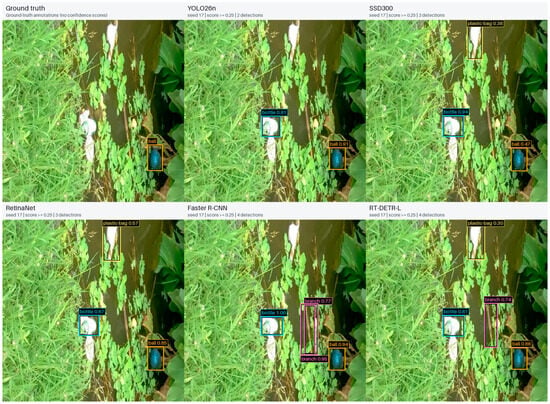
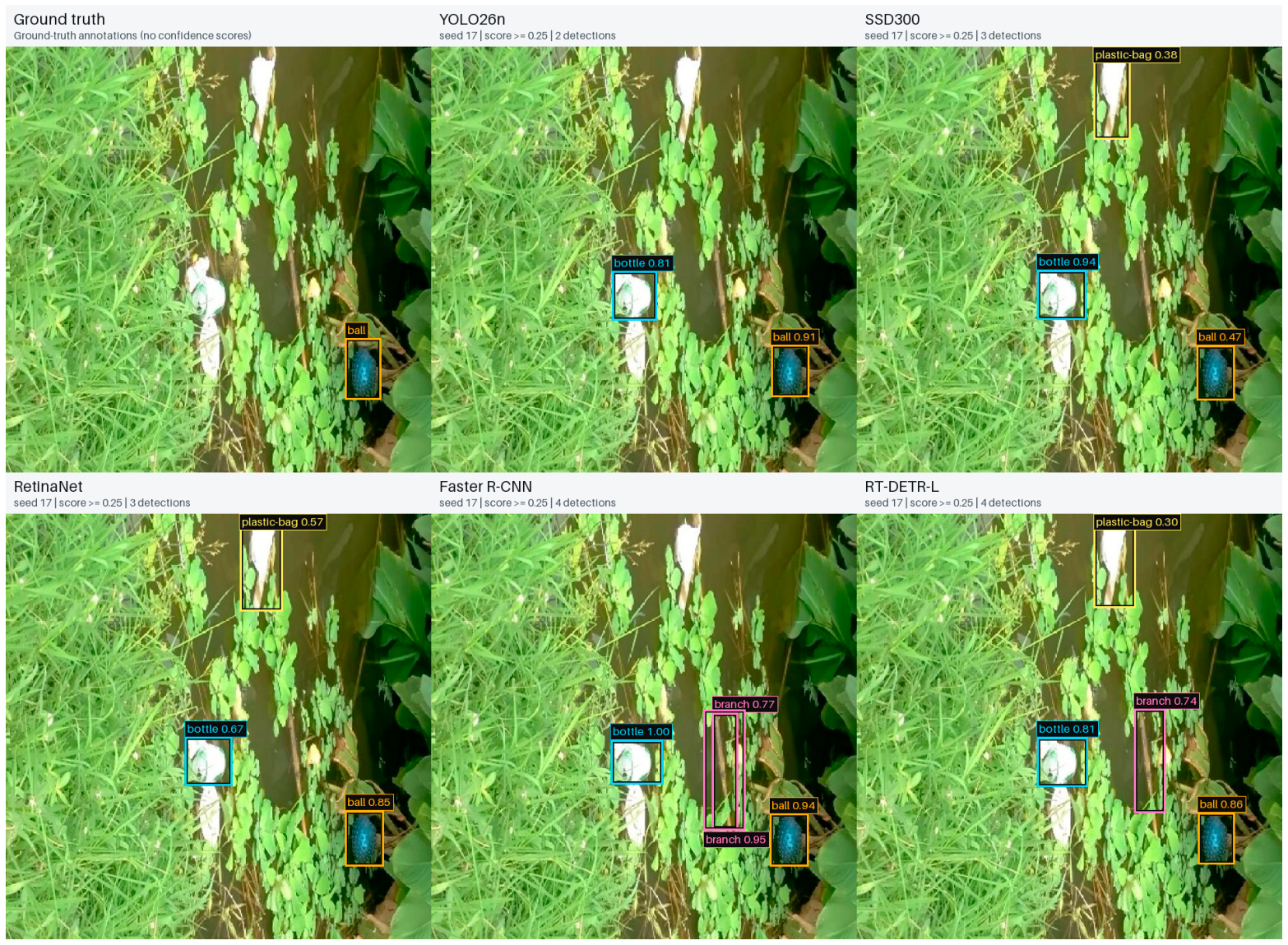
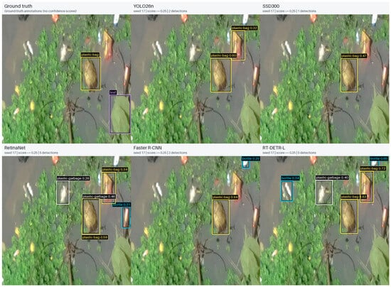
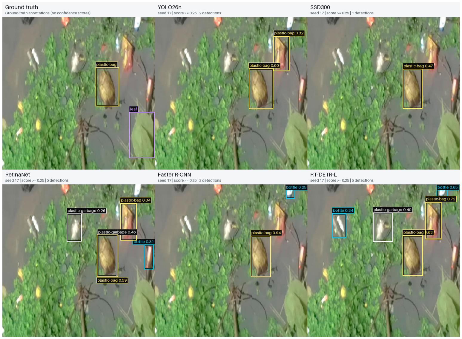
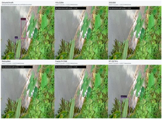
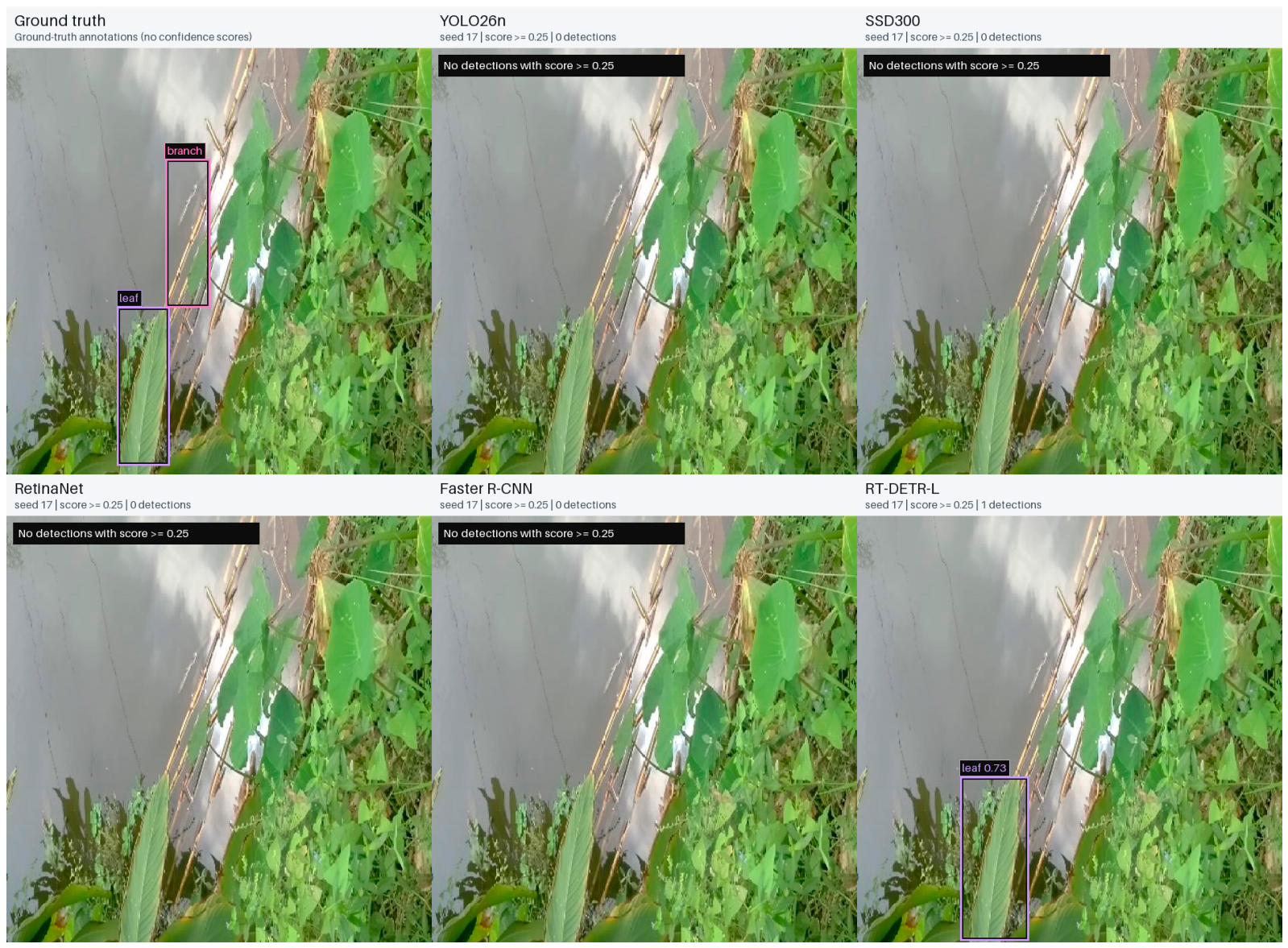

Disclaimer/Publisher’s Note: The statements, opinions and data contained in all publications are solely those of the individual author(s) and contributor(s) and not of MDPI and/or the editor(s). MDPI and/or the editor(s) disclaim responsibility for any injury to people or property resulting from any ideas, methods, instructions or products referred to in the content. |
© 2026 by the authors. Licensee MDPI, Basel, Switzerland. This article is an open access article distributed under the terms and conditions of the Creative Commons Attribution (CC BY) license.