


Abstract
Blue water is fundamental to ecological security and socioeconomic development in mountainous headwater catchments. Taking the Upper Qingjiang River Basin—a key water conservation area of the Three Gorges Reservoir—as the study area, this study develops an integrated SWAT–Geographical Detector–system dynamics framework to identify driving mechanisms and project future trends under alternative scenarios, extending previous basin studies from blue–green water scarcity to blue water volume at the township scale. Based on 2010–2022 multi-source datasets, the SWAT model provided baseline blue water estimates, the Geographical Detector quantified individual and interactive effects of ten climatic, topographic, land-use, and socioeconomic factors, and the system dynamics model simulated blue water evolution through 2030 under five scenarios. Results show that (1) natural factors dominate the spatial differentiation, with precipitation as the primary driver (mean q > 0.68) versus socioeconomic factors (max q for GDP = 0.08); (2) nonlinear enhancements prevail across factor pairs, with population–GDP interactions consistently ranking among the highest (q > 0.85 in most years); and (3) by 2030, blue water volumes rank as Ecological Conservation > Economic Prioritization > Coordinated Development > Population Growth > Baseline Development, with Ecological Conservation achieving the highest volume (471.6 million m3, 6.1% annual growth). These findings support refined water governance in Three Gorges Reservoir headwater basins.
1. Introduction
Blue water—the freshwater stored in rivers, lakes, reservoirs, and aquifers—is the most accessible renewable freshwater resource and underpins agriculture, industry, domestic supply, and riverine ecosystems [1,2,3,4]. Since the blue–green water paradigm was introduced [5], partitioning precipitation into blue water flow (runoff and deep aquifer recharge) and green water flow (evapotranspiration) has become a standard basis for water accounting [6,7]. As only about one quarter of terrestrial precipitation ultimately becomes blue water [8], and this limited resource is increasingly squeezed by population growth, economic expansion, and climate change [9,10,11], spatiotemporal imbalances in blue water availability have become a growing constraint on regional sustainable development [12]. This concern is especially relevant to the Upper Qingjiang River Basin, a key headwater conservation zone of the Three Gorges Reservoir in the karst mountainous region of western Hubei Province, whose blue water is vital to regional ecology, local livelihoods, and downstream reservoir operation [4,13]. Although relatively water abundant (mean annual precipitation of approximately 1460 mm), the basin faces pronounced rainfall variability, complex terrain, and intensifying human activities that increasingly disturb its water cycle [8,14], calling for a clear understanding of driving mechanisms, differentiated regulation, and long-term projection capabilities in line with China’s drive for ecological civilization and integrated basin management [15,16,17,18].
To address these needs, this study integrates three complementary modelling groups, each selected for a distinct analytical task against the state of the art. For blue water estimation, the Soil and Water Assessment Tool (SWAT)—the most widely applied distributed model for partitioning blue and green water at basin scales [19,20,21]—provides physically based baseline estimates of blue water flow [22,23,24]. However, most SWAT based quantifications remain at province, city, or sub-basin scales and cannot resolve intra-basin heterogeneity relevant to township-level management [25,26]; we therefore couple SWAT with a geographically weighted averaging method to disaggregate blue water estimates from sub-basins to townships—a fine-scale accounting rarely achieved in previous studies [23,27].
For driver attribution, the Geographical Detector is employed. Earlier studies typically separate natural factors (climate [28,29,30], topography [31,32], and altitude) from socio-economic factors (population [33,34], industry [35,36], and land use [37,38]) and examine their independent effects, leaving nonlinear interactions among drivers underexplored [30,39,40]. The Geographical Detector overcomes these limitations: without imposing linearity or normality assumptions, it quantifies both the individual explanatory power (q-statistic) of each factor and its pairwise interactions, and has been increasingly adopted for water-related spatial attribution [41,42,43]. Relative to earlier applications in this basin, our ten-factor system spans both natural and socio-economic groups and tracks temporal shifts in factor dominance, offering a more complete view of how multiple drivers jointly shape blue water patterns [25,32].
For future projection, a system dynamics (SD) model is constructed. Prevailing blue water studies emphasize static diagnostics, and long-term scenario simulations under alternative development pathways are seldom coupled with driver attribution [44,45,46]. SD captures feedback mechanisms within complex socio-hydrological systems and enables scenario-based simulation under multiple development orientations, with proven applications in water allocation and ecological governance [47,48,49]. Crucially, our SD model is driven by policy-adjustable socio-economic indicators—population growth, regional GDP growth, and agroforestry output—that can be actively regulated, unlike exogenous climate variables [50,51]; it thereby converts attribution results into an active planning tool.
In the Upper Qingjiang River Basin, An et al. [41] combined SWAT and the Geographical Detector to assess blue–green water scarcity and found that interaction effects outweighed single-factor effects, with socio-economic factors dominating pairwise interactions. However, that study treated blue and green water as a combined scarcity index, performed attribution at relatively coarse spatial units, and was confined to historical attribution. The present study extends it in three respects: focusing on blue water volume per se, refining the analytical resolution from sub-basins to townships, and coupling static attribution with dynamic scenario simulation in an integrated SWAT–Geographical Detector–system dynamics framework.
Accordingly, the main thread of this study is a three-step analysis in the Upper Qingjiang River Basin. Using multi-source datasets from 2010 to 2022, we first quantify blue water at the township scale by coupling SWAT with geographically weighted averaging; we then attribute its spatial heterogeneity to ten natural and socio-economic drivers and their interactions using the Geographical Detector; finally, we feed the identified drivers into a system dynamics model driven by policy-adjustable indicators to project blue water evolution through 2030 under multiple development scenarios. By bridging static attribution and dynamic forecasting, this integrated framework provides a spatially explicit, policy relevant basis for refined water management and ecological governance in the basin.
2. Materials and Methods
2.1. Study Area
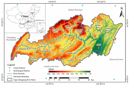
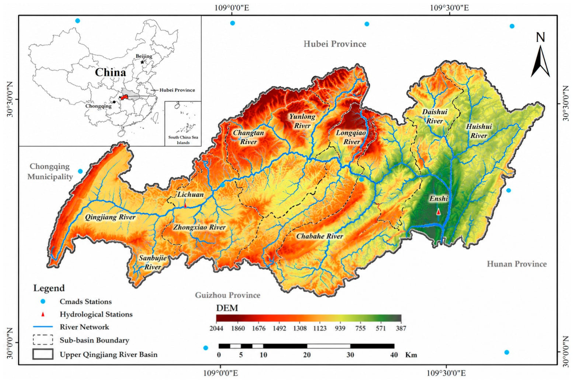
The Qingjiang River, a primary tributary of the middle Yangtze, originates in the Qiyue Mountains of Lichuan City and flows eastward through southwestern Hubei Province. Its upper reach extends approximately 153 km from the headwater to Enshi City, covering 2928 km2 (109°00′–109°59′ E, 30°12′–31°01′ N) (Figure 1). As a key headwater conservation zone of the Three Gorges Reservoir, the basin supplies blue water vital to regional ecology, local livelihoods, and downstream reservoir operation.
Figure 1.
Study area in the Upper Qingjiang River Basin.
The basin exhibits typical karst topography, with elevations ranging from 387 m to 2044 m. Under a humid subtropical monsoon climate, the mean annual temperature is 16.1 °C and the mean annual precipitation is approximately 1460 mm, more than 70% of which falls between May and September. Such pronounced seasonality, together with complex terrain and well-developed karst conduit systems, governs runoff generation and the spatiotemporal distribution of blue water. The basin is underlain by extensive karst aquifers, and groundwater constitutes a major component of its blue water resources; given the limited surface-water storage, groundwater discharge through springs and subsurface flow provides a relatively stable contribution to streamflow, particularly during the dry season. Land use is dominated by forest (60.63%) and cropland (22.26%) [52]. The reach largely spans Lichuan City and Enshi City, home to approximately 1.6 million inhabitants, with an agrarian economy based on rice, maize, and tobacco cultivation, as well as forestry, hydropower, tourism, and fisheries. According to official water statistics, residential and production water uses account for approximately 39% and 59% of total water consumption, respectively, with irrigation dominating the production component. Water is abstracted mainly through storage facilities (small reservoirs and ponds), diversion channels, and pumping stations, drawing on rivers, reservoirs, and karst springs—a pattern typical of karst mountains with limited surface water storage. Together, these hydrological conditions and water-abstraction and irrigation practices provide the empirical basis for the assumptions linking agricultural production to water use in the model, thereby supporting the rigor of the conclusions drawn from the scenario simulations.
2.2. Methods for Estimating Blue Water Resources
Blue water resources in the Upper Qingjiang River Basin were estimated through a two-stage modelling framework. First, the SWAT model was applied to simulate the basin-scale hydrological cycle and to quantify blue water at the sub-basin scale on the basis of the water balance [53,54]. Second, because SWAT outputs are aggregated at the sub-basin scale and do not correspond to township-level administrative boundaries, a geographically weighted allocation procedure was adopted to disaggregate sub-basin blue water estimates to township-level units, enabling fine-scale accounting to support differentiated water management.
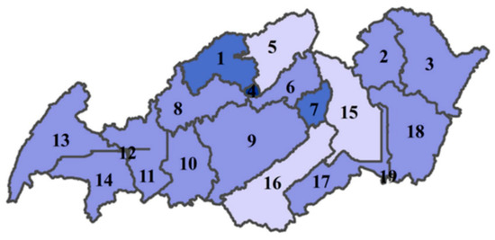
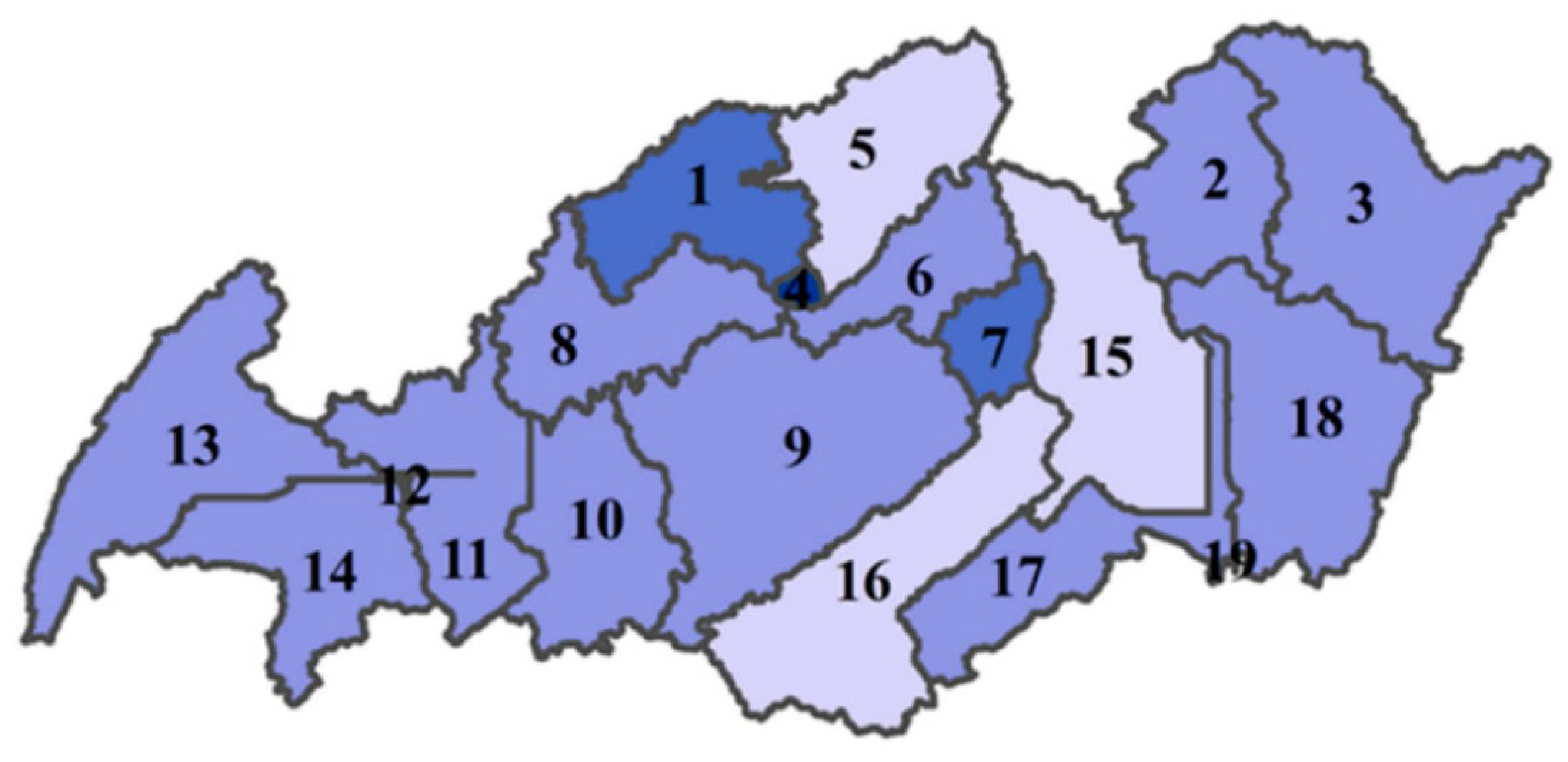
(1) SWAT model setup. The basin was discretized into 19 sub-basins from the DEM-derived drainage network (Figure 2), and each sub-basin was further subdivided into hydrological response units (HRUs) using combined thresholds of 20%, 20%, and 15% for land use, soil type, and slope class (0–10° and 10–30°), respectively, balancing simulation accuracy with computational efficiency. Potential evapotranspiration was computed with the Penman–Monteith equation, and surface runoff was estimated using the SCS curve number method; precipitation and temperature served as essential driving variables, while the remaining meteorological inputs were generated by the model’s weather generator. The weather-generator parameters are listed in Appendix A Table A1.
Figure 2.
Sub-basin division results of the SWAT model in the Upper Qingjiang River Basin.
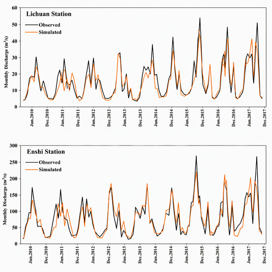
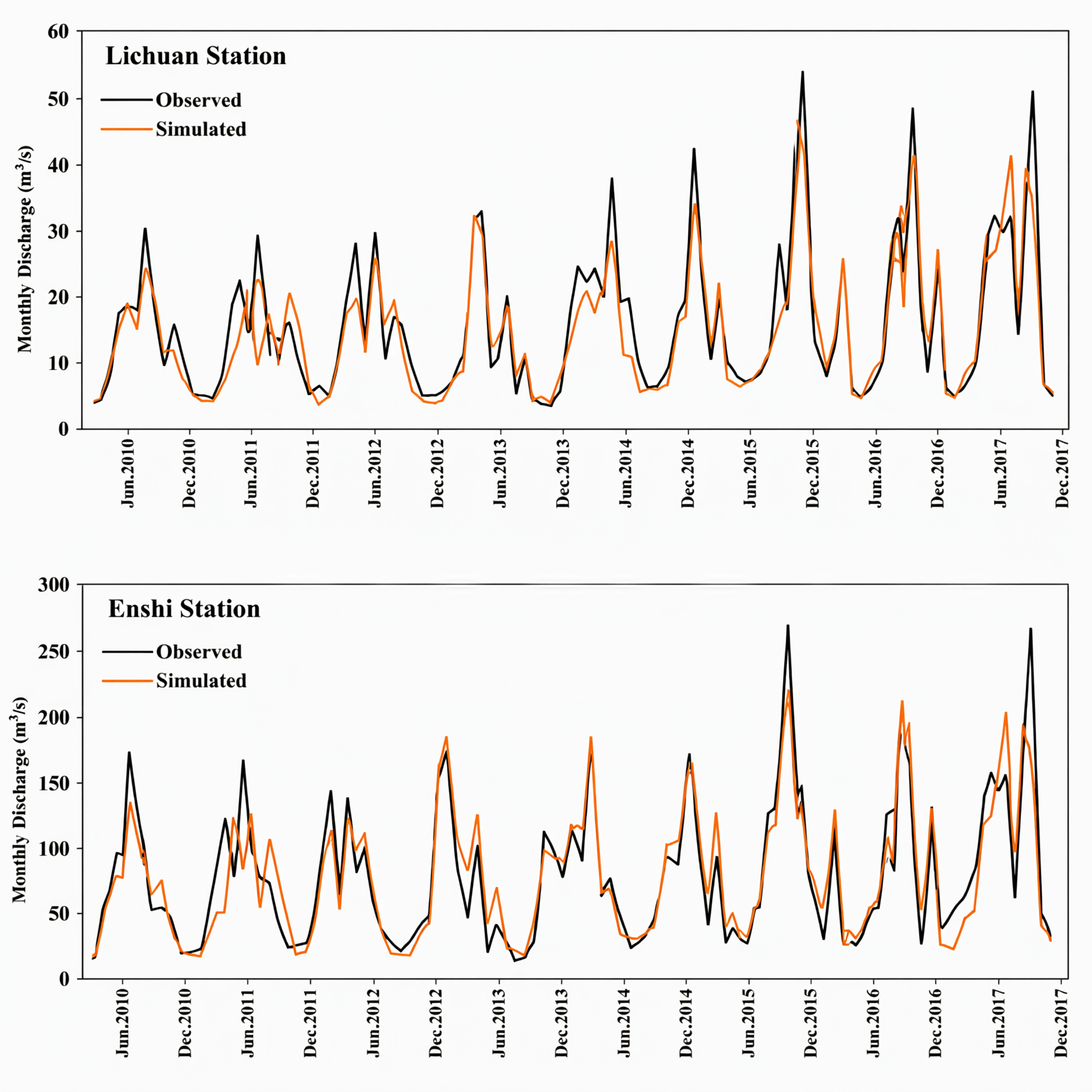
(2) Calibration and validation. The model was calibrated and validated using the SWAT Calibration and Uncertainty Program (SWAT-CUP) 5.1 with the Sequential Uncertainty Fitting (SUFI-2) algorithm, through which 16 key sensitive parameters were iteratively optimized (Appendix A Table A2). The year 2010 was defined as the one-year spin-up period to stabilize initial soil moisture and groundwater storage conditions; the calibration period spanned 2011–2016, and the independent validation period covered 2017–2018, against monthly streamflow observed at the Lichuan and Enshi stations. Model performance was evaluated using the coefficient of determination (R2), the Nash–Sutcliffe efficiency (NSE), the ratio of RMSE to the standard deviation of observations (RSR), and percent bias (PBIAS). As shown in Figure 3, the simulated hydrographs closely matched the observed streamflow at both stations during calibration and validation, and the performance metrics summarized in Table 1 confirmed the reliability of the model for blue water estimation.
Figure 3.
Simulated and observed monthly streamflow at the Lichuan and Enshi stations.
Table 1.
Performance metrics of SWAT monthly runoff simulation at Lichuan and Enshi hydrological stations.
(3) Blue water estimation. Blue water was quantified from SWAT output variables. The net water yield leaving each HRU and converging into the river through the sub-basin (WYLD, mm) is expressed as:
where SURQ, LATQ, and GWQ are surface runoff, lateral flow, and groundwater flow (mm), respectively; TLOSS is transmission loss (mm); pond is water retained by ponds and reservoirs (mm); and DA_RCHG is shallow aquifer recharge (mm). In the study basin, transmission losses are negligible and no ponds or reservoirs exist, so TLOSS ≈ 0 and pond = 0. Blue water (BW, mm) was therefore estimated as:
WYLD = SURQ + LATQ + GWQ − TLOSS − pond − DA_RCHG
BW = SURQ + LATQ + GWQ
Among these three components, groundwater flow (GWQ)—the contribution of the shallow aquifer to streamflow—constitutes an essential part of blue water resources and is particularly important in this karst-dominated basin, where subsurface pathways largely govern the hydrological response; in SWAT, this contribution is controlled by the groundwater parameters optimized during calibration (e.g., the threshold depth of water in the shallow aquifer required for return flow (GWQMN), the groundwater delay time (GW_DELAY), and the baseflow alpha factor (ALPHA_BF; Appendix A Table A2). Monthly values were then aggregated to annual values to obtain the annual blue water resource of each sub-basin over 2010–2022.
(4) Township-level spatial disaggregation. Because SWAT provides blue water estimates at the sub-basin scale, which does not match the administrative units used in local water management, a geographically weighted allocation method was applied to disaggregate sub-basin blue water to township-level units. Following the principle of geographically weighted regression (GWR) [23], spatial weights were constructed with a distance-decay function so that sub-basins closer to a given township contributed more to its blue water allocation, and the estimates were mapped onto township boundaries using GIS. The study area spans 23 townships; those with an area smaller than 20 km2 within the basin were excluded to avoid statistically unreliable estimates, leaving 19 townships for the final analysis. The resulting township-level blue water series (2010–2022) provide the basis for the subsequent spatiotemporal characterization and attribution analysis.
2.3. Geographical Detector
The spatial heterogeneity of blue water resources was attributed to candidate drivers using the Geographical Detector (GD, version 2013; Institute of Geographic Sciences and Natural Resources Research, Chinese Academy of Sciences, Beijing, China). The q-statistic (0–1) measures the explanatory power of each driver, with larger values denoting stronger effects [23,55]. Unlike conventional regression models, GD requires no linearity or normality assumptions, is insensitive to multicollinearity, and can quantify interactive effects between paired factors. Two detectors were employed: the factor detector quantifies the independent explanatory power of each driver, and the interaction detector compares the joint power of two factors against their individual powers to identify interaction types.
Table 2 lists the indicator system, with drivers grouped into socio-economic [27] and natural [56] categories. Socio-economic indicators include population density (PD), regional gross domestic product (RGDP), township economic level (TEL), forest area (FA), and agricultural area (AA). PD and RGDP were selected to represent anthropogenic water demand, since population growth and economic expansion intensify domestic, industrial, and irrigation withdrawals and compete with blue water availability [44,57]. TEL was quantified using nighttime light data owing to the scarcity of township-level economic statistics. Although FA and AA are land surface attributes, they were assigned to the socio-economic group because they are closely tied to long-term land management: agriculture consumes substantial blue water for irrigation, while forest conservation and vegetation management alter evapotranspiration and the regional water balance [40,58]. Natural factors—DEM, slope (SLP), soil organic carbon (SOC), mean annual temperature (MAT), and mean annual precipitation (MAP)—constitute the fundamental background of hydrological cycling and govern blue water generation and distribution by regulating runoff convergence, infiltration, and evapotranspiration [47,51,59].
Table 2.
Indicator System for Factors Affecting Blue Water Resources.
Compared with a previous study in the same basin that focused on the scarcity of blue and green water at relatively coarse spatial units [41], this study concentrates on blue water resources at the township scale and further applies GD to decompose the independent explanatory power of drivers and, more importantly, to quantify their nonlinear interactions. In this framework, the SWAT model and GD play complementary roles: SWAT simulates blue water through physically based hydrological processes, whereas GD quantifies the independent and interactive explanatory power of drivers. Including meteorological factors such as precipitation and temperature is not circular, as they are fundamental hydrological controls; moreover, the interaction detector captures synergistic or antagonistic effects between meteorological and other factors that SWAT alone cannot provide, offering deeper insight into the mechanisms of blue water heterogeneity.
2.4. System Dynamics Model
- (1)
- Model Framework and Subsystem Development
System dynamics (SD) relies on causal feedback loops to depict the long-term evolutionary behavior of complex socio-hydrological systems [60]. An SD model was constructed to simulate blue water variations in the Upper Qingjiang River Basin over 2010–2030, with 2010–2022 as the historical calibration stage and 2023–2030 as the scenario projection stage. The SD model deliberately centers on policy-controllable socio-economic drivers—population growth, economic expansion, and agroforestry development—while excluding climatic variables, for three reasons. First, SWAT already simulates the meteorological-driven hydrological processes, so re-including precipitation and temperature in the SD model would duplicate the physical simulation. Second, only human-oriented variables offer policy leverage: unlike precipitation and temperature, they can be regulated through planning and water governance, allowing scenario outputs to directly support decision-making. Third, the blue water equation is structurally independent of SWAT—it was fitted by regressing the historical township-scale blue water estimates (2010–2022) against socio-economic variables, and future blue water was simulated by adjusting these drivers. The regression coefficients therefore represent statistical associations rather than causal mechanisms, supporting relative scenario comparison rather than absolute prediction [50].
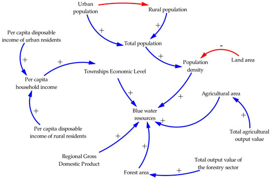
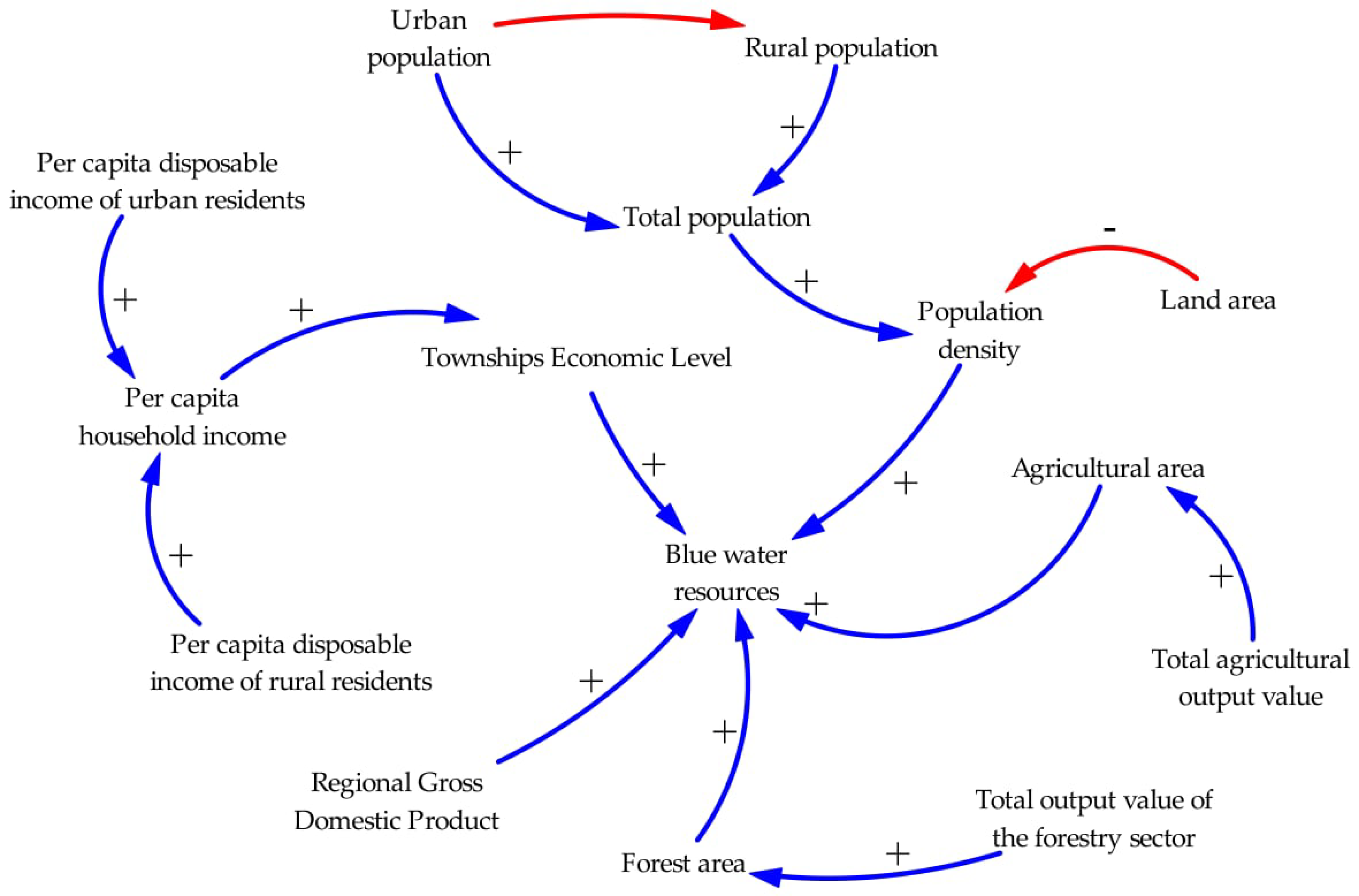
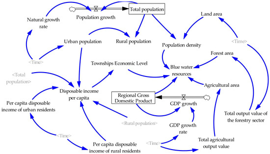
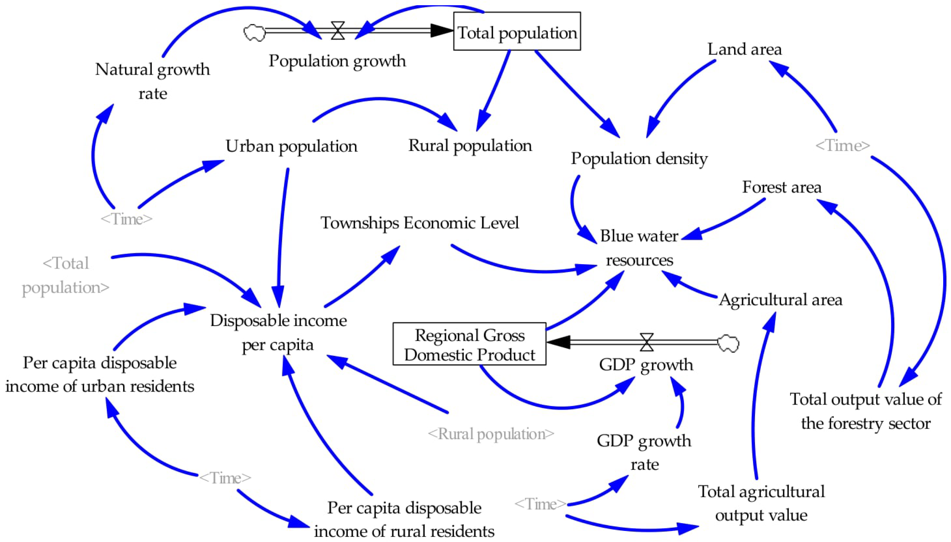
The causal loop diagram and stock-flow diagram of the model were built via Vensim PLE X32 software [61]. Figure 4 presents the causal loop diagram, where directed arrows represent variable causal linkages, with (+) denoting positive effects and (−) denoting negative effects. These signed linkages collectively form reinforcing and balancing feedback loops that reflect the inherent dynamic structure of the blue water system. Figure 5 displays the stock-flow diagram, which distinguishes state, rate, and auxiliary variables to represent the accumulation and transfer processes of blue water resources (see Appendix A Table A3 for a full list of model variables).
Figure 4.
System causal diagram for blue water allocation in the Upper Qingjiang River Basin. Blue lines with (+) denote positive effects, and red lines with (−) denote negative effects.
Figure 5.
System dynamics stock–flow diagram for blue water resources in the Upper Qingjiang River Basin.
Two strategies were adopted to calibrate model parameters: static land-use variables were assigned average values, while time-varying socio-economic indicators were extrapolated via univariate linear trend regressions (Table 3). Each equation involves a single explanatory variable and only two parameters, a low-complexity specification leaving no capacity for overfitting, which requires excessive model complexity [62]; the high R2 values therefore reflect the strong temporal trends of the drivers rather than model over-parameterization. The finalized model comprises 19 variables, with the core and key equations presented in Table 4 (full set in Appendix A Table A4).
Table 3.
Linear Regression Equations and Fitting Goodness of Socio-economic Driving Variables.
Table 4.
Main Variables and Key Equations of the System Dynamics Model for Blue Water Resources in the Upper Qingjiang River Basin.
- (2)
- Multi-Scenario Design
Blue water variations are driven by both natural conditions and human activities, with population growth, economic development, and agroforestry production recognized as the primary anthropogenic drivers of watershed-scale water consumption and scarcity [49,50]. Accordingly, three policy-adjustable indicators—natural population growth rate, RGDP growth rate, and agroforestry output growth rate—were selected as scenario variables, reflecting demographic pressure, economic status, and irrigation demand, respectively [51,59]. Baseline growth rates were set for two periods (2023–2025 and 2026–2030) based on local development cycles, official plans, and historical statistics, with low and high variants defined as population growth ±10% of the baseline, RGDP growth ±1.5 percentage points, and agroforestry output ±1 percentage point (Table 5).
Table 5.
Setting of parametric scenarios for the upper reaches in the Upper Qingjiang River Basin.
To identify plausible development pathways, low, medium, and high growth levels were set for population, GDP, and agroforestry output, generating 27 scenario combinations, with the medium level of each indicator serving as the baseline. To make the screening procedure transparent and minimize subjectivity, all 27 combinations were screened through three explicit criteria. (1) Internal consistency: combinations in which rapid population growth coexists with slow economic growth, or in which both population and economy grow slowly, were excluded because they contradict the demographic–economic pattern of Enshi Prefecture. (2) Regional adaptability: combinations with low agroforestry growth were excluded, because sustained growth of the agroforestry-dominated industrial structure is a precondition for plausible development in the basin. (3) Representativeness: among the combinations remaining after criteria (1) and (2), those whose policy implications duplicate one of the retained scenarios were excluded to avoid redundancy. The full list of the 27 combinations, together with the screening outcome and exclusion reason of each, is presented in Appendix A Table A5. After screening, five representative scenarios were retained for subsequent simulation, as listed in Table 6.
Table 6.
Scenario combinations for SD simulation in the Upper Qingjiang River Basin.
2.5. Parameters and Data Sources
The datasets employed in this research comprise a DEM covering the upstream section of the Qingjiang catchment, as well as data on land use, soil, meteorology, hydrology and the economy. Table 7 summarizes the data sources, which fall into two principal groups: statistical yearbooks and geospatial datasets. Defense Meteorological Satellite Program-Operational Linescan System (DMSP-OLS) nighttime light imagery was applied to evaluate township-level economic development across the study region. Additionally, some raw data required preprocessing prior to use, and missing entries were filled via interpolation techniques. To ensure cross-layer comparability, all spatial datasets were harmonized through a unified preprocessing chain, and the associated input uncertainties were absorbed and quantified during SWAT calibration with the SUFI-2 algorithm [63]; given the study’s focus on quantifying blue water resources and supporting relative scenario comparison rather than absolute prediction, such uncertainties do not alter the relative conclusions.
Table 7.
Data types and sources.
3. Results
3.1. Determinants of Blue Water Resource Distribution in the Upper Qingjiang River Basin
3.1.1. Analysis of the Effect of a Single Factor
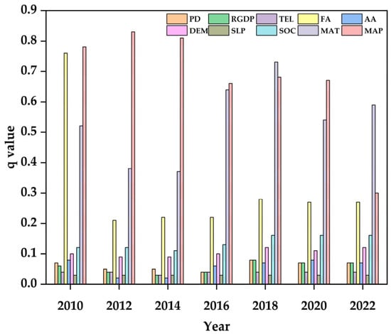
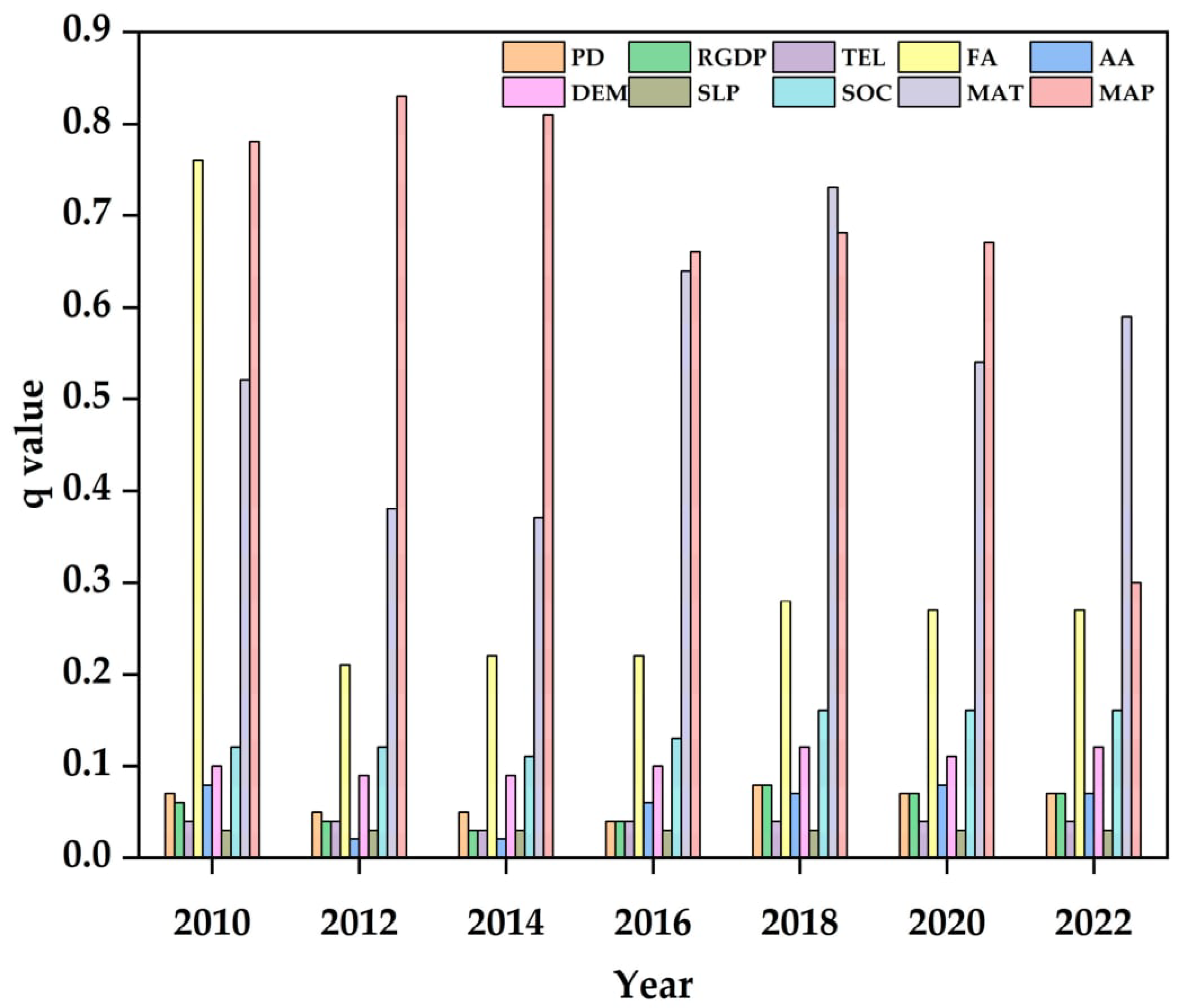
Single-factor detection reveals evident temporal variations in the explanatory power (q value) of driving factors affecting blue water resources in the Upper Qingjiang River Basin during 2010–2022 (Figure 6).
Figure 6.
Time series of single-factor q-values for blue water driving factors (2010–2022). PD, population density; RGDP, regional gross domestic product; TEL, township economic level; FA, forest area; AA, agricultural area; DEM, digital elevation model; SLP, slope; SOC, soil organic carbon; MAT, mean annual temperature; MAP, mean annual precipitation.
Overall, natural factors maintain distinctly higher explanatory capacity than socio-economic factors. Annual average precipitation (MAP) is the dominant natural driving factor, with its q value peaking at 0.83 in 2012 and remaining above 0.68 on average throughout the study period. Forest area (FA) and annual average temperature (MAT) also present relatively high explanatory power, with multi-year average q values of approximately 0.32 and 0.54, respectively, and both show periodic fluctuation characteristics.
Among socio-economic indicators, regional GDP (RGDP) serves as the most influential factor, yet its maximum q value only reaches 0.08, far lower than the peak explanatory power of annual average precipitation (MAP). Population density (PD) and township economic development level (TEL) exhibit persistently weak effects, with multi-year average q values below 0.10.
The comparison confirms that the maximum influence of the leading socio-economic factor is considerably weaker than that of the dominant natural factor. It further demonstrates that natural background conditions constitute the fundamental control over the spatial differentiation of blue water resources, whereas socio-economic factors play a secondary regulating role.
3.1.2. Analysis of the Effects of Interaction Factors
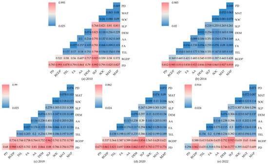
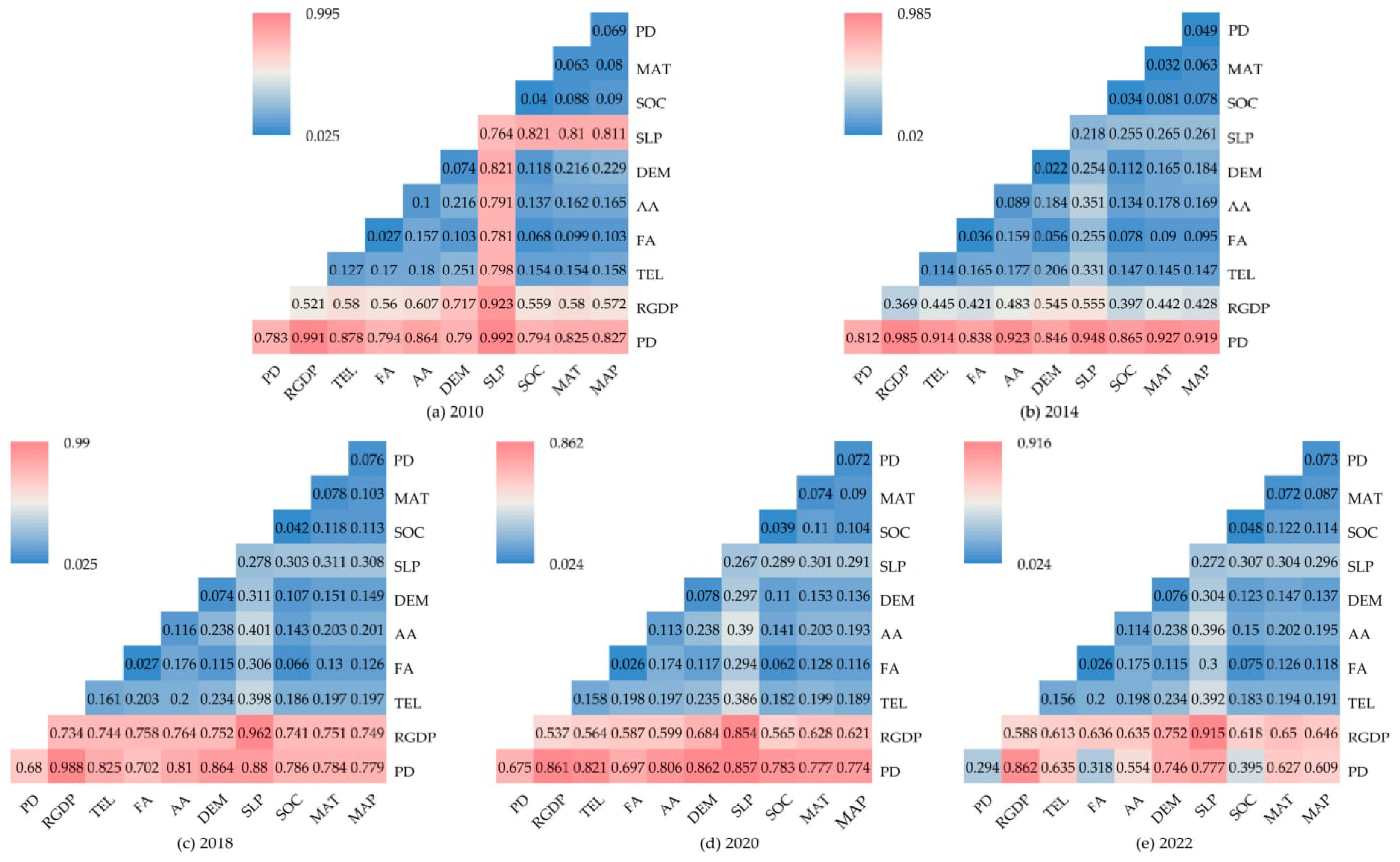
In Figure 7, color intensity represents the magnitude of q-values; a larger q-value indicates stronger explanatory power of pairwise factor interactions for the spatial variation of blue water resources. The red areas representing high q-values are mainly concentrated in the bottom rows of the matrix, dominated by interaction pairs involving socio-economic factors: population density (PD) and regional gross domestic product (RGDP).
Figure 7.
Interactive detection q-statistic matrix of driving factors affecting blue water resources in different years: (a) 2010; (b) 2014; (c) 2018; (d) 2020; (e) 2022. PD, population density; RGDP, regional gross domestic product; TEL, township economic level; FA, forest area; AA, agricultural area; DEM, digital elevation model; SLP, slope; SOC, soil organic carbon; MAT, mean annual temperature; MAP, mean annual precipitation.
In 2010, the interaction between slope (SLP) and PD exhibited the highest explanatory power, with a q-value of 0.992, followed by PD–RGDP (0.991) and SLP–RGDP (0.923); in 2014, the top-ranked interaction pairs were RGDP–PD (0.985) and SLP–PD (0.948). Meanwhile, the interaction between mean annual temperature (MAT) and PD increased notably, reaching 0.927; in 2018, RGDP–PD maintained the strongest explanatory capacity at 0.988. The leading interaction combinations were consistent with those observed in 2010, consisting of SLP–RGDP (0.962) and SLP–PD (0.880); in 2020, the dominant interaction pairs underwent obvious shifts. Digital Elevation Model (DEM)–PD became the most influential pair (0.862), followed by RGDP–PD (0.861) and SLP–PD (0.857); in 2022, the interaction between SLP and RGDP ranked first at 0.915, followed by RGDP–PD (0.862) and SLP–PD (0.777).
Three patterns emerged from the multi-year results. First, all factor pairs exhibited typical nonlinear enhancement effects, with weak standalone factors gaining substantially improved explanatory capacity after coupling with other variables. Second, a striking contrast appeared against the single-factor results: MAT and MAP, which showed prominent independent effects, achieved only modest pairwise explanatory capacity, whereas combinations containing PD and RGDP sustained high explanatory power across all years. Third, the dominant interaction pairs shifted distinctly over time, reflecting dynamic changes in the human–water system.
3.2. System Dynamics Simulation
3.2.1. Model Validation
To verify the reliability of the system dynamics simulation for blue water resources in the Upper Qingjiang River Basin, three validation approaches were implemented sequentially: operational test, stability test, and historical validation.
The operational test carried out item-by-item inspection of variable settings, data input, causal linkages and calculation equations. It also standardized variable units and simulation time parameters, focusing on easily overlooked implicit computational problems such as unit mismatches. After repeated debugging, the model operated smoothly without runtime errors. Inspection results confirmed consistent dimensional units, coherent causal relationships and valid mathematical functions within the model.
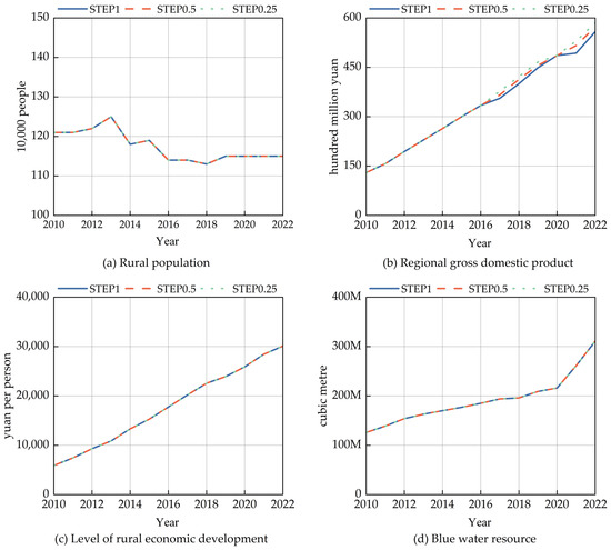
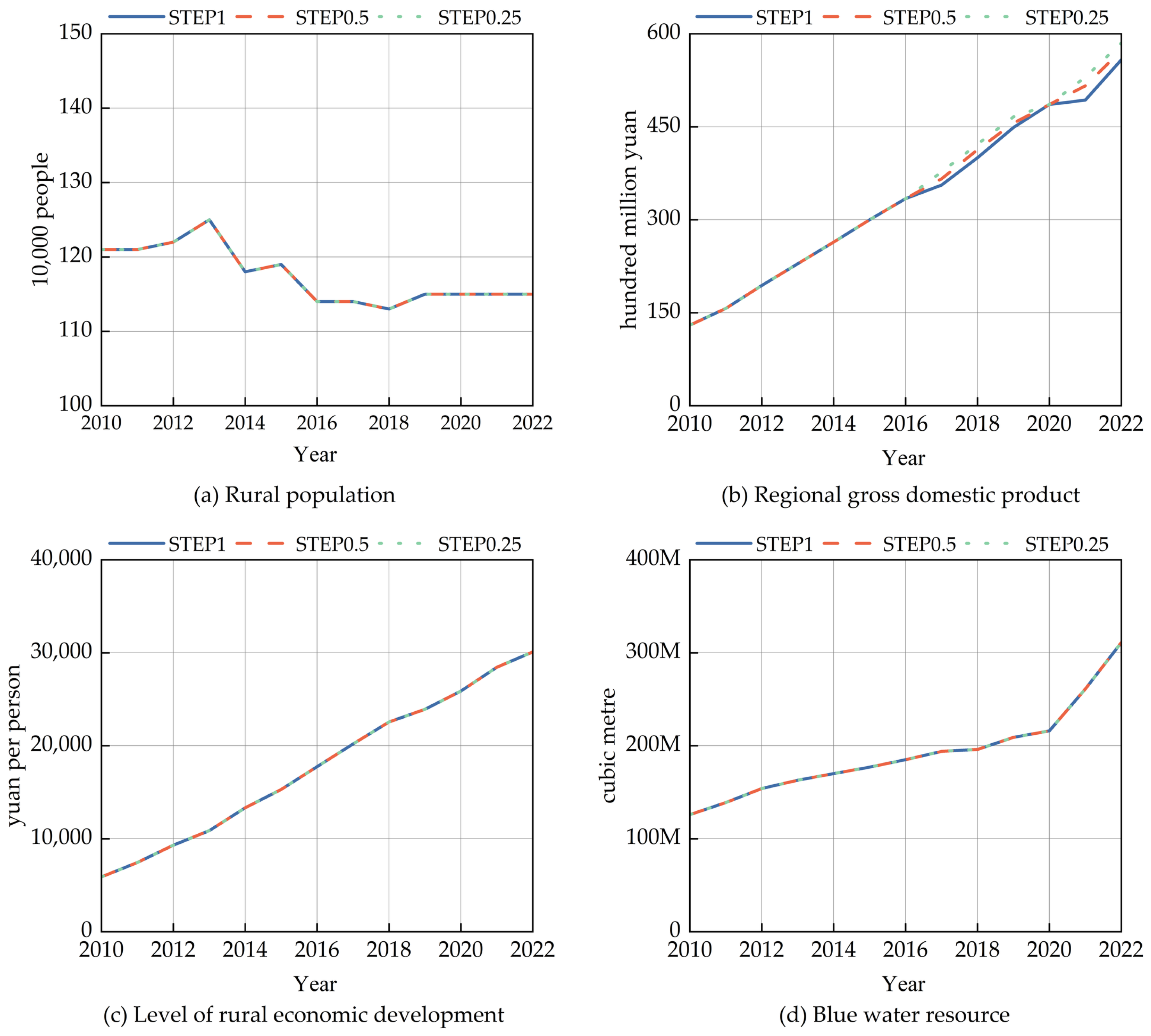
For the stability test covering the simulation period 2010–2022, three simulation time steps (1 year, 0.5 year, and 0.25 year) were configured. Simulation outputs of four core variables (rural population, regional GDP, township economic development level and blue water volume) were compared (Figure 8). The simulated trends of variables exhibited high consistency across different time steps, with only slight numerical deviations. This outcome demonstrates that the model is insensitive to disturbances of time-discrete parameters and possesses favorable structural stability.
Figure 8.
Temporal evolution of socio-economic indicators and blue water resources (2010–2022) under different simulation time steps. (a) Rural population; (b) Regional gross domestic product; (c) Level of rural economic development; (d) Blue water resources. STEP1, STEP0.5 and STEP0.25 denote system dynamics simulation time steps of 1 a, 0.5 a and 0.25 a.
To further verify the reliability of the constructed system dynamics framework, a historical validation was conducted over the 2010–2022 period using three representative variables: township economic development level, agricultural output value, and blue water resources. The simulated values were generated by the system dynamics model and compared with observed data (Table 8), and the overall performance was further quantified using summary metrics—mean absolute error (MAE), root mean square error (RMSE), mean absolute percentage error (MAPE), and Nash–Sutcliffe efficiency (NSE)—as summarized in Table 9. The observed values for township economic development level and agricultural output value were obtained from statistical records, providing an independent validation of the model’s ability to reproduce real socioeconomic conditions.
Table 8.
Results of historical testing of the model.
Table 9.
Performance metrics of the SD model in historical validation.
For blue water resources, no township-level observational dataset exists; the estimates were derived from SWAT outputs downscaled using the geographically weighted average method. Because these SWAT-derived estimates were also used to calibrate the system dynamics equation, the blue water comparison is a behavioral validation—it tests whether the model reproduces the historical trend of the physically based benchmark—rather than an independent validation. Importantly, the SWAT model itself was calibrated and validated against observed monthly streamflow at two hydrological stations, so the blue water benchmark is physically constrained by field measurements. The relative errors for all three variables remained within ±10% (mostly below 5%), and the summary metrics (Table 9) further confirmed the satisfactory performance of the model, demonstrating that it reproduces historical trends and provides a sound basis for relative scenario comparison.
3.2.2. Simulation Analysis
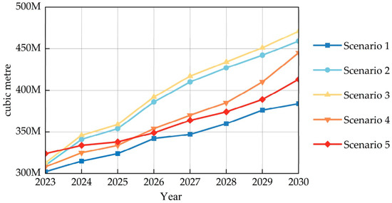
Marked differences in blue water resource accumulation were observed across the five combined scenarios (Figure 9), corresponding to the scenario settings listed in Table 6.
Figure 9.
Temporal variations of blue water resources under five differentiated development scenarios (Scenario 1: Baseline Development; Scenario 2: Economic Prioritization; Scenario 3: Ecological Conservation; Scenario 4: Coordinated Development; Scenario 5: Population Growth).
Scenario 1 (Baseline Development scenario): Medium growth rates are adopted for population, GDP and total forestry output. This scenario yields the lowest volume of blue water resources throughout the simulation period.
Scenario 2 (Economic Prioritization scenario): This scheme sets low population growth alongside high growth rates of GDP and forestry output. Blue water resources experience a slight decline in 2024 compared with 2023 in the early simulation stage, followed by continuous growth, and reach 459.6 million m3 by 2030, ranking second among all scenarios. This early decline is consistent with rising water demand during rapid economic expansion, followed by recovery driven by technological progress and ecological investment—in line with the EKC pattern discussed below.
Scenario 3 (Ecological Conservation scenario): Population density and GDP maintain medium growth, while forestry output grows rapidly. Blue water resources rise steadily from 311.6 million m3 in 2023 to 471.6 million m3 in 2030, with an annual growth rate of approximately 6.1%, ranking first across all scenarios. The result reveals that prioritizing ecological protection effectively facilitates the continuous accumulation of blue water resources.
Scenario 4 (Coordinated Development scenario): Medium growth rates are applied to population and forestry output, while GDP grows at a low rate. Blue water resources reach 445.4 million m3 by 2030, ranking third. This scenario strikes a balance between economic progress and ecological protection and possesses strong practical operability.
Scenario 5 (Population Growth scenario): A high natural population growth rate is configured, with medium growth for GDP and forestry output. Its simulated blue water volume ranks fourth.
Overall, the ranking of simulated blue water volume by 2030 is as follows: Scenario 3 (Ecological Conservation) > Scenario 2 (Economic Prioritization) > Scenario 4 (Coordinated Development) > Scenario 5 (Population Growth) > Scenario 1 (Baseline Development). In general, strengthened ecological conservation contributes to higher blue water storage capacity.
4. Discussion
4.1. Mechanism Interpretation and Theoretical Anchoring
In the Upper Qingjiang River Basin, natural factors dominate the spatial heterogeneity of blue water, with precipitation being the primary source of water supply and temperature controlling evapotranspiration; both serve as core climatic drivers [30,32]. Although these are input variables for the SWAT model, the geographical detector provides unique quantitative attribution results. The model quantifies the explanatory power of each independent factor at the township level through q-values and p-values, and captures the spatiotemporal variations in the dominance of individual factors—information that cannot be obtained solely through SWAT process simulation.
Between 2010 and 2022, there were significant changes in the dominant natural drivers. In the early years, precipitation was the primary driver of blue water recharge, which is consistent with findings from studies of subtropical mountain catchments [28,30]. Persistent regional warming exacerbated spatial variations in evapotranspiration, and the single-factor detection results (Figure 6) indicate that temperature became the dominant factor over the most recent three years: the explanatory power of precipitation declined sharply from 0.67 (2020) to 0.30 (2022), while temperature remained relatively high (0.54 and 0.59) and surpassed precipitation in 2022 (0.59 vs. 0.30); this reflects the dynamic response of the hydrological system to climate change [29]. Forest cover plays a significant regulatory role in infiltration and water resource conservation [47], reshaping the ‘blue water’ regime in complex mountainous terrain [32,37]. The relationship between vegetation and water varies significantly depending on climate and land use [38]; dense canopies and thick layers of dead branches and fallen leaves may reduce total water yield by limiting infiltration [41,48]. The positive water-retention effect of the forest in this study stems from the humid subtropical, energy-limited environment of the catchment, where infiltration and groundwater recharge exceed transpiration losses [50,64]. This contrasts with conditions in arid catchments, where afforestation may actually exacerbate water scarcity [44,57].
In summary, the natural context fundamentally determines the spatial variation in ‘blue water’, whilst socio-economic factors (population density, economic level of towns and villages) play a weaker, secondary role.
4.2. Implications of Multi-Factor Synergistic Effects
Notably, the interaction q-values approaching unity were almost exclusively associated with pairs coupling socio-economic factors (PD, RGDP) with topographic factors (SLP, DEM), whereas climatic pairs remained modest. This selective concentration reflects genuine synergistic effects rather than artifacts of data structure or discretization: PD and RGDP, weak in isolation, gained markedly when combined with terrain-related factors, which is consistent with the spatially coupled distribution of population, economy, and topography—settlements and cropland tend to concentrate in gentle-slope zones. Moreover, the temporal consistency of these dominant PD-/RGDP-based pairs across all years further supports the robustness of the identified synergies.
Comparison with previous studies. The interaction-dominance pattern identified here aligns with An et al. [41], who reported a similar finding for blue–green water scarcity in the same basin; our results extend it to blue water volume, confirming its robustness across different dependent variables. The combined roles of climatic and human factors are also evident in Liang et al. [30], who showed, for the rapidly developing Xiangjiang River Basin, that blue water scarcity was jointly driven by precipitation (r = 0.425) and population (r = −0.612), underscoring that no single factor alone governs water scarcity. Similarly, socio-economic factors were found to explain 71% of aquatic spatial variation versus only 9% for climatic factors in another study [40]. The widespread nonlinear enhancement effects further corroborate prior blue water research [44,58]—for example, the explanatory power of population density rises from 0.37 alone to 0.74 in interaction [25]. Together, these comparisons support our core inference that, although climatic variables dominate individually, socio-economic factors become the leading restrictive forces under multi-factor interactions—a perspective that SWAT-based analyses focusing on single-factor sensitivity cannot provide [65].
The geographically weighted disaggregation introduces some uncertainty related to the mismatch between sub-basin and township boundaries; however, because the procedure preserves sub-basin totals and subsequent analyses rely on relative comparisons, this uncertainty does not alter the main conclusions.
4.3. Enlightenment from Multi-Scenario Simulation and Policy Pathways
Unlike SWAT-based projections of blue water under changing climate and land use [66,67,68], this study uses a system dynamics (SD) approach focusing on socio-economic drivers. Climate and land use are largely exogenous and can only be responded to, whereas socio-economic factors—population growth, GDP growth, and agroforestry output—are policy-adjustable. The model therefore serves as an active planning tool, evaluating what can be achieved through targeted policy interventions rather than passively forecasting external changes.
The five scenarios yielded distinct blue water trajectories. Scenario 1 (Baseline) maintained the lowest volume throughout. Scenario 2 (Economic Prioritization) declined slightly in 2024 and then grew to 459.6 million m3 by 2030 (second), a “decline-then-grow” pattern consistent with the Environmental Kuznets Curve [50,58]. Scenario 3 (Ecological Conservation) achieved the highest volume (471.6 million m3, 6.1% annual growth), confirming the effectiveness of nature-based measures [69,70]. Scenario 4 (Coordinated Development) ranked third (445.4 million m3), balancing economic and ecological objectives [44,71]. Scenario 5 (Population Growth) ranked fourth, as rising demand restricted accumulation. Overall, greater ecological governance yields higher blue water accumulation; results should be read as a comparative assessment of development pathways rather than exact forecasts.
A methodological limitation should be acknowledged: the historical blue water used to calibrate the SD model derives from the same SWAT–GWR chain, so the calibration period is not an entirely independent validation. This mainly constrains confidence in absolute volumes for 2023–2030; relative comparisons across scenarios are largely unaffected, as systematic biases would be common to all scenarios and cancel out in ranking. The SWAT estimates themselves were validated against observed streamflow with satisfactory metrics, providing independent anchoring; future work could add water-resources-bulletin or remote-sensing data for cross-validation.
Taken together, the present study extends An et al. [41] by shifting the focus from blue–green water scarcity to blue water volume, expanding the driver system, and coupling static attribution with dynamic scenario simulation. The consistent interaction-dominance pattern identified in both studies reinforces the robustness of the findings, while the system dynamics extension offers a forward-looking tool for policy evaluation.
5. Conclusions
This study developed an integrated SWAT–Geographical Detector–system dynamics framework to estimate blue water resources, attribute their spatial differentiation, and project their evolution under five scenarios in the Upper Qingjiang River Basin. Three management implications follow. First, ecological governance—preserving forest cover, soil water retention, and headwater conservation capacity—is the primary lever for safeguarding blue water, given the dominance of natural drivers. In particular, groundwater, a critical component of blue water resources in this karst basin, warrants dedicated attention in water management and conservation. Second, the strong interactions between socio-economic and topographic factors imply that single-factor policies are insufficient; integrated, multi-objective watershed governance at the township level is required. Third, scenario simulation identifies ecological conservation as the optimal pathway, whereas economic-prioritization and population-growth pathways intensify water pressure, supporting differentiated regional management.
Methodologically, the framework offers a transferable paradigm for blue water research in data-similar mountainous headwater catchments, extending conventional single-factor sensitivity analyses through township-level downscaling and the dynamic coupling of static attribution with scenario simulation; parameter values remain context-dependent and require recalibration elsewhere. Future work should refine blue water estimation with higher-resolution remote sensing data, extend the driver system, incorporate climatic variables as dynamic inputs into the system dynamics model, and cross-validate estimates against independent water-resources-bulletin or remote-sensing data.
Author Contributions
Conceptualization, X.M.; methodology, X.M.; software, X.M.; validation, X.M.; formal analysis, X.M.; investigation, X.M.; resources, S.D.; data curation, S.D.; writing—original draft preparation, W.X.; writing—review and editing, W.X.; visualization, X.M.; supervision, W.X.; project administration, W.X.; funding acquisition, W.X. All authors have read and agreed to the published version of the manuscript.
Funding
This research was funded by the National Natural Science Foundation of China (Youth Program), grant number 72004116.
Data Availability Statement
The variable definitions, system dynamics model equations, causal loop diagram, stock-flow diagram, and scenario settings are fully documented in the main text (Table 3, Table 4, Table 5 and Table 6, Figure 4 and Figure 5) and Appendix A. The SWAT model configuration files and the full set of calibrated parameter values are not included in the manuscript due to the extensive technical documentation required; these materials are available from the corresponding author upon reasonable request. The meteorological, hydrological, land use, soil, and socioeconomic data used in this study were obtained from publicly accessible sources, as summarized in Table 7. The Geodetector software (version 2013) used for factor detection is freely available at http://www.geodetector.cn/ (accessed on 20 October 2026). No proprietary or restricted datasets were used in this study.
Acknowledgments
We also sincerely thank the editor and the three anonymous reviewers for their valuable comments and suggestions, which have significantly improved the quality of this manuscript.
Conflicts of Interest
The authors declare no conflicts of interest. The funders had no role in the design of the study; in the collection, analyses, or interpretation of data; in the writing of the manuscript; or in the decision to publish the results.
Appendix A
Table A1.
Parameters and definitions of the weather generator database in the SWAT model.
Table A2.
Calibrated sensitive parameters of the SWAT model for the Upper Qingjiang River Basin.
Table A3.
Key Variables in the Blue Water Resources System of the Upper Qingjiang River Basin.
Table A4.
Variables and Equations of the System Dynamics Model for Blue Water Resources in the Upper Qingjiang River Basin.
Table A5.
Screening of the 27 scenario combinations: outcomes and exclusion reasons.
References
- Hoekstra, A.Y. Green-Blue Water Accounting in a Soil Water Balance. Adv. Water Resour. 2019, 129, 112–117. [Google Scholar] [CrossRef] [Scilit]
- Intergovernmental Panel on Climate Change. Climate Change 2007: Impacts, Adaptation and Vulnerability; Intergovernmental Panel on Climate Change: Genebra, Suíça, 2001. [Google Scholar]
- Heselschwerdt, S.P.; Wagener, T.; Wang-Erlandsson, L.; Ukkola, A.M.; Markonis, Y.; Yang, Y.; Greve, P. Large Impact of Extreme Precipitation on Projected Blue-Green Water Partitioning. Earth Syst. Dyn. 2026, 17, 811–827. Available online: https://esd.copernicus.org/articles/17/811/2026 (accessed on 20 October 2026). [CrossRef] [Scilit]
- Deng, Q.; Sharretts, T.; Ali, T.; Ao, Y.Z.; Chiarelli, D.D.; Demeke, B.; Marston, L.; Mehta, P.; Mekonnen, M.; Rulli, M.C. Deepening Water Scarcity in Breadbasket Nations. Nat. Commun. 2025, 16, 1110. [Google Scholar] [CrossRef] [Scilit]
- Falkenmark, M.; Rockström, J. The New Blue and Green Water Paradigm: Breaking New Ground for Water Resources Planning and Management. J. Water Resour. Plan. Manag. 2006, 132, 129–132. [Google Scholar] [CrossRef] [Scilit]
- Wu, J.; Deng, G.; Zhou, D.; Zhu, X.; Ma, J.; Cen, G.; Jin, Y.; Zhang, J. Effects of Climate Change and Land-Use Changes on Spatiotemporal Distributions of Blue Water and Green Water in Ningxia, Northwest China. J. Arid Land 2021, 13, 674–687. [Google Scholar] [CrossRef] [Scilit]
- Zang, C.; Liu, J. Trend Analysis for the Flows of Green and Blue Water in the Heihe River Basin, Northwestern China. J. Hydrol. 2013, 502, 27–36. [Google Scholar] [CrossRef] [Scilit]
- Wang-Erlandsson, L.; Tobian, A.; van der Ent, R.J.; Fetzer, I.; te Wierik, S.; Porkka, M.; Staal, A.; Jaramillo, F.; Dahlmann, H.; Singh, C.; et al. A Planetary Boundary for Green Water. Nat. Rev. Earth Environ. 2022, 3, 380–392. [Google Scholar] [CrossRef] [Scilit]
- Cárdenas Belleza, G.A.; van Beek, L.R.; Bierkens, M.F.; Jones, E.R.; van Vliet, M.T. Sector-Specific Clean Water Scarcity and Competition under Global Change. npj Clean Water 2026, 9, 58. [Google Scholar] [CrossRef] [Scilit]
- Wen, Z.; Yi, S.; Sun, W. Significant Contribution of the Tianshan Lakes to Their Water Storage and Water Resources. J. Hydrol. Reg. Stud. 2024, 53, 101813. [Google Scholar] [CrossRef] [Scilit]
- Khadem, M.; Rougé, C.; Harou, J.J.; Hansen, K.M.; Medellin-Azuara, J.; Lund, J.R. Estimating the Economic Value of Interannual Reservoir Storage in Water Resource Systems. Water Resour. Res. 2018, 54, 8890–8908. [Google Scholar] [CrossRef] [Scilit]
- Ding, B.; Zhang, J.; Zheng, P.; Li, Z.; Wang, Y.; Jia, G.; Yu, X. Water Security Assessment for Effective Water Resource Management Based on Multi-Temporal Blue and Green Water Footprints. J. Hydrol. 2024, 632, 130761. [Google Scholar] [CrossRef] [Scilit]
- Li, Y.; Huang, R.; Meng, H.; Soomro, S.; Zhang, H.; Guo, J.; Li, C.; Wang, Y. Power Generation Dispatching and Risk Analysis of the Qingjiang Cascade Hydropower Stations under Climate Change. J. Water Clim. Change 2025, 16, 380–399. [Google Scholar] [CrossRef] [Scilit]
- Tan, X.; Liu, B.; Tan, X.; Huang, Z.; Fu, J. Combined Impacts of Climate Change and Human Activities on Blue and Green Water Resources in a High-Intensity Development Watershed. Hydrol. Earth Syst. Sci. 2025, 29, 427–445. [Google Scholar] [CrossRef] [Scilit]
- Wang, X.; Gao, J.; Jiang, H.; Li, S. Construction of Evaluation Index System of Water Resources Carrying Capacity Based on Ecological Civilization. Front. Environ. Sci. 2025, 13, 1524894. [Google Scholar] [CrossRef] [Scilit]
- Guan, D.; Chen, S.; Zhang, Y.; Liu, Z.; Peng, G.; Zhou, L. Influencing Factors and the Establishment of a Basin Ecological Compensation Mechanism from the Perspective of Water Conservation: A Case Study of the Upper Yangtze River in China. J. Clean. Prod. 2024, 456, 142332. [Google Scholar] [CrossRef] [Scilit]
- Xu, Z.; Cheng, L.; Liu, P.; Hou, Q.; Cheng, S.; Qin, S.; Liu, L.; Xia, J. Investigating the Spatial Variability of Water Security Risk and Its Driving Mechanisms in China Using Machine Learning. J. Clean. Prod. 2022, 362, 132303. [Google Scholar] [CrossRef] [Scilit]
- Song, X.; Ravesteijn, W.; Frostell, B.; Wennersten, R. Managing Water Resources for Sustainable Development: The Case of Integrated River Basin Management in China. Water Sci. Technol. 2010, 61, 499–506. [Google Scholar] [CrossRef] [Scilit]
- Zhang, X.; Jiang, C.; Huang, J.; Ni, Z.; Sun, J.; Li, Z.; Wen, T. Spatiotemporal Evaluation of Blue and Green Water in Xinjiang River Basin Based on SWAT Model. Water 2022, 14, 2429. [Google Scholar] [CrossRef] [Scilit]
- Liu, M.; Wang, D.; Chen, X.; Chen, Y.; Gao, L.; Deng, H. Impacts of Climate Variability and Land Use on the Blue and Green Water Resources in a Subtropical Basin of China. Sci. Rep. 2022, 12, 20993. [Google Scholar] [CrossRef] [Scilit]
- Jeyrani, F.; Morid, S.; Srinivasan, R. Assessing Basin Blue–Green Available Water Components under Different Management and Climate Scenarios Using SWAT. Agric. Water Manag 2021, 256, 107074. [Google Scholar] [CrossRef] [Scilit]
- Xie, P.; Zhuo, L.; Yang, X.; Huang, H.; Gao, X.; Wu, P. Spatial-Temporal Variations in Blue and Green Water Resources, Water Footprints and Water Scarcities in a Large River Basin: A Case for the Yellow River Basin. J. Hydrol. 2020, 590, 125222. [Google Scholar] [CrossRef] [Scilit]
- Wang, J.-F.; Li, X.-H.; Christakos, G.; Liao, Y.-L.; Zhang, T.; Gu, X.; Zheng, X.-Y. Geographical Detectors-Based Health Risk Assessment and Its Application in the Neural Tube Defects Study of the Heshun Region, China. Int. J. Geogr. Inf. Sci. 2010, 24, 107–127. [Google Scholar] [CrossRef] [Scilit]
- Veettil, A.V.; Mishra, A.K. Water Security Assessment Using Blue and Green Water Footprint Concepts. J. Hydrol. 2016, 542, 589–602. [Google Scholar] [CrossRef] [Scilit]
- Zhang, L.; Li, N.; Beng, V. Impact of Spatial Scale on the Sensitivity of the Water Supply-Demand Balance to Driving Factors. Ecol. Indic. 2026, 185, 114744. [Google Scholar] [CrossRef] [Scilit]
- Noorduijn, S.L.; Refsgaard, J.C.; Petersen, R.J.; Højberg, A.L. Downscaling a National Hydrological Model to Subgrid Scale. J. Hydrol. 2021, 603, 126796. [Google Scholar] [CrossRef] [Scilit]
- Gu, Y.; Shao, Z.; Huang, X.; Cai, B. GDP Forecasting Model for China’s Provinces Using Nighttime Light Remote Sensing Data. Remote Sens. 2022, 14, 3671. [Google Scholar] [CrossRef] [Scilit]
- Padhiary, J.; Patra, K.C.; Dash, S.S.; Uday Kumar, A. Climate Change Impact Assessment on Hydrological Fluxes Based on Ensemble GCM Outputs: A Case Study in Eastern Indian River Basin. J. Water Clim. Change 2020, 11, 1676–1694. [Google Scholar] [CrossRef] [Scilit]
- Ray Biswas, R.; Sharma, R.; Gyasi-Agyei, Y.; Rahman, A. Urban Water Security: Water Supply and Demand Management Strategies in the Face of Climate Change. Urban Water J. 2023, 20, 723–737. [Google Scholar] [CrossRef] [Scilit]
- Liang, J.; Liu, Q.; Zhang, H.; Li, X.; Qian, Z.; Lei, M.; Li, X.; Peng, Y.; Li, S.; Zeng, G. Interactive Effects of Climate Variability and Human Activities on Blue and Green Water Scarcity in Rapidly Developing Watershed. J. Clean. Prod. 2020, 265, 121834. [Google Scholar] [CrossRef] [Scilit]
- Liu, M.; Ye, Z.; He, P.; Yang, S.; Zhang, Y.; Zhou, C.; Zhang, Y.; Gan, X.; Qin, X. Relations of Residential Green and Blue Spaces with New-Onset Chronic Kidney Disease. Sci. Total Environ. 2023, 869, 161788. [Google Scholar] [CrossRef] [Scilit]
- Liu, H.; Hui, S.; Zhao, Y.; Jiang, Y.; Qi, Y.; Boyer, E.W.; Mello, C.R.; Guo, L.; Li, H. Spatiotemporal Variability of Soil Moisture and Its Influencing Factors in a Forested Catchment with Complex Terrain. CATENA 2025, 256, 109079. [Google Scholar] [CrossRef] [Scilit]
- Yang, X.; Zhuo, L.; Xie, P.; Huang, H.; Feng, B.; Wu, P. Physical versus Economic Water Footprints in Crop Production: A Spatial and Temporal Analysis for China. Hydrol. Earth Syst. Sci. 2021, 25, 169–191. [Google Scholar] [CrossRef] [Scilit]
- Ssekyanzi, G.; Ahmad, M.J.; Choi, K.-S. Sustainable Solutions for Mitigating Water Scarcity in Developing Countries: A Comprehensive Review of Innovative Rainwater Storage Systems. Water 2024, 16, 2394. [Google Scholar] [CrossRef] [Scilit]
- Zeng, W.; He, J.; Qiu, Y.; Cao, X. Unravelling the Temporal-Spatial Distribution of the Agricultural Water Footprint in the Yangtze River Basin (YRB) of China. Water 2021, 13, 2562. [Google Scholar] [CrossRef] [Scilit]
- Xiao, X.; Su, Y. Application of Water Resource Economic Management Model in Agricultural Structure Adjustment. Water Supply 2023, 23, 3832–3843. [Google Scholar] [CrossRef] [Scilit]
- Woldesenbet, T. Impact of Land Use and Land Cover Dynamics on Ecologically-Relevant Flows and Blue-Green Water Resources. Ecohydrol. Hydrobiol. 2022, 22, 420–434. [Google Scholar] [CrossRef] [Scilit]
- Msigwa, A.; Komakech, H.C.; Salvadore, E.; Seyoum, S.; Mul, M.L.; van Griensven, A. Comparison of Blue and Green Water Fluxes for Different Land Use Classes in a Semi-Arid Cultivated Catchment Using Remote Sensing. J. Hydrol. Reg. Stud. 2021, 36, 100860. [Google Scholar] [CrossRef] [Scilit]
- Chai, C.; Wang, L.; Chen, D.; Zhou, J.; Li, N.; Liu, H. Quantifying Future Water Resource Vulnerability in a High-Mountain Third Pole River Basin under Climate Change. J. Environ. Manag. 2024, 367, 121954. [Google Scholar] [CrossRef] [Scilit]
- Zhou, C.; Xie, Y.; Zhang, A.; Liu, C.; Yang, J. Spatiotemporal Analysis of Interactions between Seasonal Water, Climate, Land Use, Policy, and Socioeconomic Changes: Hulun-Buir Steppe as a Case Study. Water Res. 2022, 209, 117937. [Google Scholar] [CrossRef] [Scilit]
- An, M.; Xu, W.; Fang, X.; Cheng, C.; Ramsey, T.S. The Measure of Scarcity of Blue and Green Water and Its Driving Factors via the SWAT Model: An Application to the Upper Qingjiang River, China. Irrig. Drain. 2025, 74, 1803–1817. [Google Scholar] [CrossRef] [Scilit]
- Ansari Mahabadi, S.; Delavar, M. Evaluation and Comparison of Different Methods for Determining the Contribution of Climatic Factors and Direct Human Interventions in Reducing Watershed Discharge. Ecol. Indic. 2024, 158, 111480. [Google Scholar] [CrossRef] [Scilit]
- Jin, T.; Zhang, X.; Wang, T.; Liang, J.; Ma, W.; Xie, J. Spatiotemporal Impacts of Climate Change and Human Activities on Blue and Green Water Resources in Northwest River Basins of China. Ecol. Indic. 2024, 160, 111823. [Google Scholar] [CrossRef] [Scilit]
- Liu, Y.; Jing, Y.; Han, S. Multi-Scenario Simulation of Land Use/Land Cover Change and Water Yield Evaluation Coupled with the GMOP-PLUS-InVEST Model: A Case Study of the Nansi Lake Basin in China. Ecol. Indic. 2023, 155, 110926. [Google Scholar] [CrossRef] [Scilit]
- Tang, J.; Song, P.; Hu, X.; Chen, C.; Wei, B.; Zhao, S. Coupled Effects of Land Use and Climate Change on Water Supply in SSP–RCP Scenarios: A Case Study of the Ganjiang River Basin, China. Ecol. Indic. 2023, 154, 110745. [Google Scholar] [CrossRef] [Scilit]
- Fang, C.; Cui, X.; Li, G.; Bao, C.; Wang, Z.; Ma, H.; Sun, S.; Liu, H.; Luo, K.; Ren, Y. Modeling Regional Sustainable Development Scenarios Using the Urbanization and Eco-Environment Coupler: Case Study of Beijing Tianjin-Hebei Urban Agglomeration, China. Sci. Total Environ. 2019, 689, 820–830. [Google Scholar] [CrossRef] [Scilit]
- Chen, J.; Wang, D.; Li, G.; Sun, Z.; Wang, X.; Zhang, X.; Zhang, W. Spatial and Temporal Heterogeneity Analysis of Water Conservation in Beijing-Tianjin-Hebei Urban Agglomeration Based on the Geodetector and Spatial Elastic Coefficient Trajectory Models. GeoHealth 2020, 4, e2020GH000248. [Google Scholar] [CrossRef] [Scilit]
- Yang, L.; Yang, X.; Wei, W.; Pan, J. Spatio-Temporal Evolution and Influencing Factors of Water Resource Carrying Capacity in Shiyang River Basin: Based on the Geographical Detector Method. Water Supply 2020, 20, 1409–1424. [Google Scholar] [CrossRef] [Scilit]
- Soligno, I.; Malik, A.; Lenzen, M. Socioeconomic Drivers of Global Blue Water Use. Water Resour. Res. 2019, 55, 5650–5664. [Google Scholar] [CrossRef] [Scilit]
- Huang, X.; Chen, X. A Regional Eco-Compensation Assessment Framework for Blue Water Scarcity Based on the Spatial Effects of Socio-Economic Factors. J. Clean. Prod. 2022, 368, 133171. [Google Scholar] [CrossRef] [Scilit]
- Yin, S.; Dongjie, G.; Weici, S.; Weijun, G. Integrated Assessment and Scenarios Simulation of Urban Water Security System in the Southwest of China with System Dynamics Analysis. Water Sci. Technol. 2017, 76, 2255–2267. [Google Scholar] [CrossRef] [Scilit]
- Lin, Z.; Ye, X.; Wei, Q.; Xin, F.; Lu, Z.; Kudva, S.; Dai, Q. Ecosystem Services Value Assessment and Uneven Development of the Qingjiang River Basin in China. Sustainability 2017, 9, 2356. [Google Scholar] [CrossRef] [Scilit]
- Ahmad, S.; Shazil, M.S.; Mahmood, S.A.; Abdullah-Al-Wadud, M.; Tariq, A. Quantifying Climate Change Impacts on Hydrological Dynamics and Sedimentation Using GIS and SWAT plus Modelling. Hydrol. Process. 2025, 39, e70082. [Google Scholar] [CrossRef] [Scilit]
- Tan, M.L.; Gassman, P.W.; Yang, X.; Haywood, J. A Review of SWAT Applications, Performance and Future Needs for Simulation of Hydro-Climatic Extremes. Adv. Water Resour. 2020, 143, 103662. [Google Scholar] [CrossRef] [Scilit]
- da Silva, A.R.; Lima, A.d.O. Geographically Weighted Beta Regression. Spat. Stat. 2017, 21, 279–303. [Google Scholar] [CrossRef] [Scilit]
- Stonefelt, M.; Fontaine, T.; Hotchkiss, R. Impacts of Climate Change on Water Yield in the Upper Wind River Basin. JAWRA J. Am. Water Resour. Assoc. 2000, 36, 321–336. [Google Scholar] [CrossRef] [Scilit]
- Yuan, Z.; Xu, J.; Xu, D.; Liu, S.; Fan, B.; Li, X. The Carbon Emissions Risk Evolution and Low-Carbon Optimization in a Typical Mountainous Region on the Western Edge of the Sichuan Basin, China. Ecol. Indic. 2024, 162, 112064. [Google Scholar] [CrossRef] [Scilit]
- Liu, M.; Dong, X.; Zhang, Y.; Wang, X.; Wei, H.; Zhang, P.; Zhang, Y. Spatiotemporal Changes in Future Water Yield and the Driving Factors under the Carbon Neutrality Target in Qinghai. Ecol. Indic. 2024, 158, 111310. [Google Scholar] [CrossRef] [Scilit]
- Sun, Y.; Liu, N.; Shang, J.; Zhang, J. Sustainable Utilization of Water Resources in China: A System Dynamics Model. J. Clean. Prod. 2017, 142, 613–625. [Google Scholar] [CrossRef] [Scilit]
- Wei, S.; Yang, H.; Song, J.; Abbaspour, K.C.; Xu, Z. System Dynamics Simulation Model for Assessing Socio-Economic Impacts of Different Levels of Environmental Flow Allocation in the Weihe River Basin, China. Eur. J. Oper. Res. 2012, 221, 248–262. [Google Scholar] [CrossRef] [Scilit]
- Mashaly, A.F.; Fernald, A.G. Identifying Capabilities and Potentials of System Dynamics in Hydrology and Water Resources as a Promising Modeling Approach for Water Management. Water 2020, 12, 1432. [Google Scholar] [CrossRef] [Scilit]
- Hawkins, D.M. The Problem of Overfitting. J. Chem. Inf. Comput. Sci. 2004, 44, 1–12. [Google Scholar] [CrossRef] [Scilit]
- Abbaspour, K.C.; Rouholahnejad, E.; Vaghefi, S.; Srinivasan, R.; Yang, H.; Kløve, B. A Continental-Scale Hydrology and Water Quality Model for Europe: Calibration and Uncertainty of a High-Resolution Large-Scale SWAT Model. J. Hydrol. 2015, 524, 733–752. [Google Scholar] [CrossRef] [Scilit]
- Veettil, A.V.; Mishra, A. Water Security Assessment for the Contiguous United States Using Water Footprint Concepts. Geophys. Res. Lett. 2020, 47, e2020GL087061. [Google Scholar] [CrossRef] [Scilit]
- Yuan, Z.; Xu, J.; Meng, X.; Wang, Y.; Yan, B.; Hong, X. Impact of Climate Variability on Blue and Green Water Flows in the Erhai Lake Basin of Southwest China. Water 2019, 11, 424. [Google Scholar] [CrossRef] [Scilit]
- Wang, S.; Zhang, H.-J.; Wang, T.-T.; Hossain, S. Simulating Runoff Changes and Evaluating under Climate Change Using CMIP6 Data and the Optimal SWAT Model: A Case Study. Sci. Rep. 2024, 14, 23228. [Google Scholar] [CrossRef] [Scilit]
- Ougahi, J.; Karim, S.; Mahmood, S. Application of the SWAT Model to Assess Climate and Land Use/Cover Change Impacts on Water Balance Components of the Kabul River Basin, Afghanistan. J. Water Clim. Change 2022, 13, 3977–3999. [Google Scholar] [CrossRef] [Scilit]
- Tao, J.; Cao, Y.; Gan, R.; Zuo, Q.; Zhao, Q.; He, Y. Impacts of Land Use and Climate Change on Runoff in the Shaying River Basin Based on SWAT Model. Limnology 2024, 25, 155–170. [Google Scholar] [CrossRef] [Scilit]
- Willis, K.J.; Petrokofsky, G. The Natural Capital of City Trees. Science 2017, 356, 374–376. [Google Scholar] [CrossRef] [Scilit]
- Yuan, L.; Geng, M.; Li, F.; Xie, Y.; Tian, T.; Chen, Q. Spatiotemporal Characteristics and Drivers of Ecosystem Service Interactions in the Dongting Lake Basin. Sci. Total Environ. 2024, 926, 172012. [Google Scholar] [CrossRef] [Scilit]
- Nie, W.; Xu, B.; Ma, S.; Yang, F.; Shi, Y.; Liu, B.; Hao, N.; Wu, R.; Lin, W.; Bao, Z. Coupling an Ecological Network with Multi-Scenario Land Use Simulation: An Ecological Spatial Constraint Approach. Remote Sens. 2022, 14, 6099. [Google Scholar] [CrossRef] [Scilit]

Disclaimer/Publisher’s Note: The statements, opinions and data contained in all publications are solely those of the individual author(s) and contributor(s) and not of MDPI and/or the editor(s). MDPI and/or the editor(s) disclaim responsibility for any injury to people or property resulting from any ideas, methods, instructions or products referred to in the content. |
© 2026 by the authors. Licensee MDPI, Basel, Switzerland. This article is an open access article distributed under the terms and conditions of the Creative Commons Attribution (CC BY) license.