


Abstract
Flood forecasting is essential for managing hydrological conditions and providing early disaster warnings. While many studies integrate data with machine learning models for flood prediction, the development of predictive models is limited when data is insufficient. Combining existing data with hydrological and hydraulic models and machine learning provides an effective method for flood prediction. In this study, the simulation results of HEC-HMS and HEC-RAS were used to simplify modeling and flood prediction in the study area using the Crossformer deep learning model. The HEC-HMS and HEC-RAS models were used to simulate the existing data and generate additional flood scenarios. The Crossformer model was applied to learn from the simulation results, establishing a fast and accurate prediction model. The Crossformer model achieved an R2 score of 0.970 and an MAE of 0.043, demonstrating high predictive accuracy in engineering applications. This study will provide a theoretical basis for the creation of rapid prediction models for river flooding with small data samples.
1. Introduction
Floods are one of the most common and destructive natural disasters that pose significant threats to human societies [1]. These events cause considerable loss of life, population displacement, and economic damage worldwide [2]. Continued global warming is projected to increase human exposure to climate extremes, including river floods [3]. The flood risks and economic impacts of the above issues are more severe in some developing countries [4]. Effective adaptation measures are therefore essential for reducing flood vulnerability and associated losses [5]. In recent years, model-based prediction of the timing, location, duration, and potential impacts of floods has played a crucial role in disaster risk reduction, safeguarding lives and property, and urban planning [6].
Traditional flood forecasting methods rely primarily on hydrological and meteorological models, including physics-based models, empirical statistical models, and numerical weather prediction models. Physically based hydrological and hydrodynamic modeling enables prediction of rainfall–runoff processes and flood flows in watersheds. Hydrodynamic simulations typically require solving partial differential equations and can be computationally demanding, especially when simulating urban areas [7]. Empirical statistical models, such as multiple regression and autoregressive moving average (ARMA) models, establish predictive relationships for predicting flood discharge through historical data analysis. While these models have lower computational costs, their predictive performance depends on the quality and representativeness of historical data [8]. To address the above challenges, the integration of machine learning (ML) with hydraulic simulation software has demonstrated significant potential in flood forecasting and water resource management. For instance, an integrated LSTM–CNN framework has been developed to emulate HEC-RAS 1D/2D simulations, supporting river water-level prediction and flood inundation mapping with reduced computational demands [9]. Furthermore, frameworks modeling compound floods by integrating river flow and rainfall effects have yielded results consistent with observed water levels and inundation depths [10]. Overall, the integration of ML with hydraulic simulation software significantly enhances the accuracy of water resource management and flood forecasting.
For further advancements, deep learning models based on ML have been developed that are capable of automatic feature extraction and processing of high-dimensional data. Deep learning models excel at uncovering complex relationships within intricate data structures, often outperforming traditional ML approaches. Compared to physics-based hydrodynamic models, deep learning-driven methods effectively and adaptively extract complex system input–output relationships [11]. For example, integrating neural networks into distributed process-based hydrological models has improved the representation of internal hydrological fluxes and flood modelling performance [12]. Beyond simulating core hydrological processes, deep learning has also proven valuable in applications such as flood inundation prediction. An enhanced U-Net architecture, FloodUnet, has enabled rapid spatiotemporal prediction of flood depth and inundation extent [13]. A Transformer model combined with Long Short-Term Memory (LSTM) networks could enhance flood forecasting accuracy by leveraging spatial and temporal data [14]. Additionally, Transformers have outperformed recurrent neural networks in predicting next-day river levels using past upstream tributary data [15].
Recent studies in civil engineering have combined machine learning with optimization techniques for predictive modelling. In geotechnical engineering, a stacking ensemble model incorporating Bayesian optimization for hyperparameter tuning achieved better predictive performance than the individual classifiers evaluated for soil liquefaction prediction [16]. For urban flood modelling, a CNN–RNN framework was developed to fuse spatial and temporal features. Bayesian optimization was used to identify influential input factors and their combinations, while LSTM–DeepLabv3+ was identified as the best-performing architecture among the combinations evaluated [17]. For hydrological forecasting, the Xinanjiang hydrological model was coupled with LSTM-based residual correction, with particle swarm optimization and Bayesian optimization employed for model calibration [18]. These studies motivate consideration of model architecture, input selection, and parameter optimization when developing hydrological forecasting frameworks.
Crossformer extends the Transformer architecture by incorporating Dimension-Segment-Wise (DSW) Embedding, a Two-Stage Attention (TSA) Layer, and a Hierarchical Encoder–Decoder (HED), enabling the representation of temporal and cross-dimensional dependencies in multivariate time series [19]. These capabilities make Crossformer a promising approach for multivariate flood forecasting. Recent advances have demonstrated the effectiveness of deep learning surrogates trained on HEC-RAS simulations [20] and adaptive urban flood prediction incorporating Crossformer-based water-level forecasting [21]. However, in sparsely monitored river reaches, limited flood records constrain the development and evaluation of data-driven models, while the computational demands of repeated hydraulic simulations pose challenges for timely flood assessment. The potential of simulation-generated data to support joint forecasting of precipitation, discharge, and water depth remains insufficiently explored. These challenges highlight the pressing need for an integrated framework that combines hydrological and hydraulic scenario simulations with efficient multivariate forecasting to capture temporal and cross-variable dependencies and provide timely information for flood assessment and mitigation planning.
To address these gaps, this study develops a simulation-assisted forecasting framework integrating HEC-HMS, HEC-RAS, and Crossformer for river reaches with limited flood observations. Its methodological contribution lies in linking scenario-based rainfall–runoff and channel–floodplain simulations with joint multivariate sequence prediction. The assembled precipitation, discharge, and four water-depth series are used to develop a Bayesian-optimized Crossformer that represents temporal and cross-variable dependencies within a unified forecasting model. Model performance is evaluated using held-out simulated conditions and an independent observed flood event, while execution-time comparisons are conducted to assess computational efficiency. The proposed framework provides a practical means of rapidly predicting multiple flood-related variables, offering information to support decision-makers in assessing river flood conditions and planning appropriate mitigation measures.
2. Study Area and Data
2.1. Study Area
The study area is situated in northern Qingdao City, spanning geographical coordinates ranging from 36°11′ N to 36°24′ N latitude and 120°07′ E to 120°34′ E longitude. It extends 41.5 km at its maximum east–west width and 24 km north–south, covering a total area of 520.24 km2 (Figure S1). The terrain in this region is complex and varied: low mountains and hills dominate the eastern part and flat plains characterize the central zone, while low-lying coastal wetlands define the western and northern parts. This configuration forms a stepped topography with higher elevations in the east, flat terrain centrally, and lower elevations westward.
Located at the transitional boundary between the subtropical and temperate zones, the region features a temperate monsoon continental climate with distinct seasons and mild conditions. Diverse soil types occur across the area, where the mean annual temperature ranges between 11 °C and 12 °C. Most rivers are monsoon-driven, precipitation-fed systems. The mild and humid climate supports the growth of both southern and northern plant species, though complex terrain results in uneven vegetation density distribution.
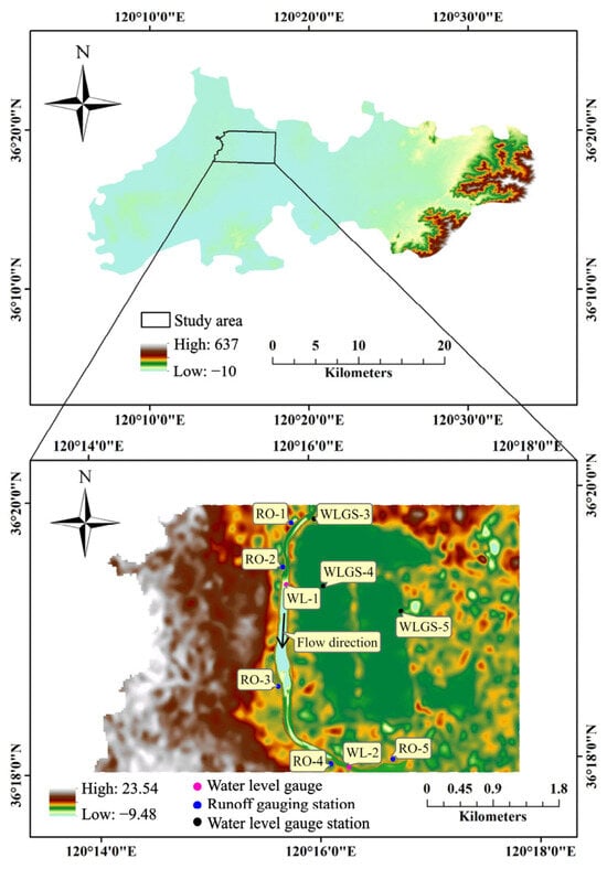
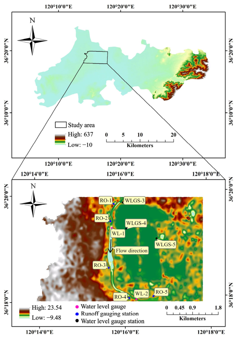
The study reach is situated predominantly within wetland parkland, with limited residential development. The river flow direction and monitoring station locations are shown in Figure 1. The study reach is not affected by tidal action, and its previous flood-protection standard corresponded to a return period of approximately 50 years. River overtopping during heavy rainfall on 25 June 2022 and 22 August 2023 affected low-lying areas along the right bank. According to the available reports, maximum inundation depths did not exceed 0.50 m during either event, and the impacts on local residents and property were limited.
Figure 1.
Location and DEM of the study area.
2.2. Geometric Data
The study utilized both actual engineering data and a digital elevation model (DEM) (Figure 1). The actual engineering data comprise river layout plans, earthwork cross-sections, and standard cross-sections for bank slope protection. Geometric information was extracted from the river construction plans and cross-sectional construction diagrams using ArcGIS Pro (version 3.1.5). These diagrams provide crucial details on the actual location and shape of key structural features, including the specific elevations of cross-sections and construction material information. These details are essential for simulating river flow and determining channel roughness.
Through detailed analysis of the construction diagrams and plan cross-sections, the location and structure of each cross-section were precisely defined, including the specific types of materials used [22]. The choice of these materials significantly influences channel surface roughness. For example, different construction materials such as concrete, stone, or clay exhibit markedly different surface roughness, which directly affects water flow velocity and direction [23]. Furthermore, integrating these engineering data enables more accurate simulation and prediction of regional hydrological conditions, especially for flood simulation and management. Accurate topographic and geomorphologic data, combined with comprehensive information on channel structures, provide a robust foundation for establishing and validating HEC-HMS and HEC-RAS models [24]. Integrating DEM and actual engineering data for modeling improved the accuracy of model predictions from topographic files and also demonstrated a more comprehensive visualization of hydrologic features [25].
2.3. Hydrological Data
Observed precipitation, discharge, and water-level records were obtained through field monitoring by the XM hydrological station and its integrated monitoring system. The monitoring archive covered the period from 11 March 2022 to 1 November 2023. These observations supported the calibration and validation of the hydrological and hydraulic models. Five rainfall–runoff events with relatively complete records were selected for analysis: 9 June 2022, 25 June 2022, 14 August 2022, 22 August 2023 and 28 September 2023. Event selection was based on record availability and completeness. The selected events cover different observed rainfall–runoff responses and include the two 2022–2023 events associated with reported right-bank inundation, providing cases for model development and evaluation under the monitored hydrological conditions. Utilizing these data, HEC-HMS and HEC-RAS models were established and validated. Because the available observed rainfall events did not adequately cover storms of different magnitudes, synthetic design storms were generated for return periods of 1, 5, 10, 50, and 100 years. The rainstorm intensity formula revised for Qingdao in 2015 was adopted:
where q is the design rainfall intensity [L/(s ⋅ ha)], P is the return period (years), and t is the rainfall duration (min). The corresponding mean rainfall intensity in mm/min was calculated as:
As shown in Figure S2, rainfall intensity increased with the return period, while the temporal position of the rainfall peak remained unchanged. These design storms were subsequently used to drive the rainfall–runoff simulations in HEC-HMS.
Watershed delineation was performed in ArcGIS using a 1-m resolution DEM, generating a sub-watershed map. The spatial distribution of the Curve Number (CN) was then derived using the Soil Conservation Service Curve Number (SCS-CN) method. Spatial inputs for the HEC-HMS model comprised the data of land cover and soil classification (Figure S3). For the HEC-RAS model, spatial inputs included river channel geometry data extracted from engineering drawings, DEM (Figure S1), land cover data (Figure S3a), and soil classification data (Figure S3b). The sources, spatial and temporal characteristics, and applications of the datasets are summarized in Table 1. With these detailed data and model construction, it is possible to accurately simulate the rainfall–runoff process.
Table 1.
Summary of the datasets used in model development and evaluation.
3. Methodology
The proposed framework comprises HEC-HMS (version 4.12), HEC-RAS (version 6.6), and Crossformer. HEC-HMS generates discharge hydrographs for the specified rainfall scenarios, which are supplied to HEC-RAS to simulate the hydraulic responses of the river and floodplain. The corresponding precipitation forcing, discharge series, and water-depth series are assembled into a multivariate dataset for Crossformer. Crossformer learns the temporal relationships in these sequences and uses the preceding 64 time steps to jointly forecast the subsequent four steps of the six variables. Its performance is evaluated separately using held-out simulated conditions and an observed flood event.
3.1. Hydrological Model
HEC-HMS, a hydrological modeling system developed by the Hydrologic Engineering Center of the U.S. Army Corps of Engineers (USACE), simulates key hydrological processes. It is primarily applied for rainfall–runoff modeling, flood forecasting, watershed management, and water resources planning [26]. The HEC-HMS model offers considerable flexibility in simulating diverse processes, including rainfall–runoff, river flow routing, and evapotranspiration [27]. Its modular design allows users to select appropriate sub-models and parameters, and its intuitive interface facilitates model construction and result analysis [28].
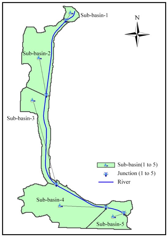
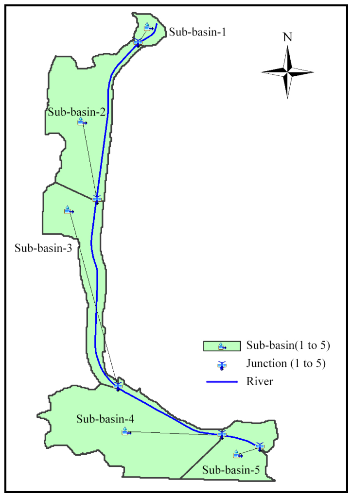
Spatial data for hydrological modeling were first processed and integrated in the HEC-HMS hydrological model (Figure 2). The study catchment was selected because available field surveys, river-engineering records, and rainfall–runoff observations supported model construction and calibration. A 1 m-resolution DEM was processed in ArcGIS to delineate the drainage boundary, river network, and five sub-catchments according to topographic divides and flow-routing relationships. The delineation was checked against field survey and engineering data, and sub-catchment areas were corrected where necessary. Thus, the computational domain represents the surface-drainage area contributing to the selected outlet, rather than an arbitrarily selected area surrounding the river. For rainfall–runoff modeling, this domain was treated as a single outlet-controlled hydrological unit, assuming no surface-runoff transfers across its external boundary. The five sub-catchments are connected through reaches and junctions, rather than being five isolated watersheds.
Figure 2.
Hydrologic model in HEC-HMS.
The rainfall–runoff response is mainly affected by rainfall intensity and temporal distribution, drainage area, terrain slope, flow-path length, land use, soil properties, antecedent moisture conditions, and channel-routing characteristics. In the HEC-HMS model, the effects of land use and soil properties were represented by the spatially distributed SCS curve number, hillslope runoff transformation was simulated using the SCS unit hydrograph method, and river routing was represented using the Muskingum–Cunge method. Accordingly, the curve number, sub-basin lag time, channel length, channel slope, and Manning’s roughness coefficient were considered the principal parameters controlling runoff volume, peak discharge, and peak timing.
The model parameters were calibrated by comparing simulated and observed rainfall–runoff processes. The computational time step was selected to resolve rainfall inputs and runoff responses. Following calibration, the model was driven by the 1-, 5-, 10-, 50-, and 100-year design rainfall events. The resulting discharge hydrographs were supplied to HEC-RAS to extend the range of simulated flood scenarios.
3.2. Hydraulic Model
HEC-RAS, developed by the USACE, is versatile software used for managing and controlling rivers, channels, harbors, and other public works. It supports a variety of simulations, including one-dimensional (1D) steady flow, 1D and two-dimensional (2D) unsteady flow, sediment transport, movable bed computations, and water temperature/water quality modeling [29,30]. Primarily employed in floodplain management and flood insurance studies, the model is essential for evaluating floodway encroachment impacts [31]. Its implementation could enhance the precision of flood risk management.
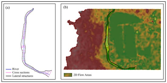
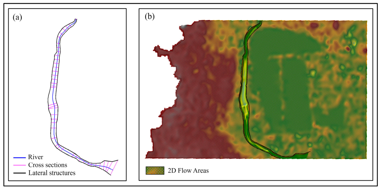
The HEC-RAS model was constructed using river discharge, precipitation, water-level observations, and geometric data. A 1 m-resolution DEM provided the baseline terrain, supplemented by river-layout drawings, engineering cross sections, and bank-protection drawings to refine the representation of the river channel. Riverbed elevations, cross-sectional shapes, and bank elevations were incorporated into the 1D channel geometry, while surrounding terrain elevations were used to define the 2D floodplain domain. The 1D model simulated flow within the main channel (Figure 3a), and the 2D model simulated inundation in the adjacent floodplain (Figure 3b). The two domains were connected through lateral structures to represent channel–floodplain flow exchange. The hydraulic simulations used to generate the Crossformer training samples were therefore performed using the specified river geometry and terrain.
Figure 3.
1D (a) and 2D (b) hydraulic model in HEC-RAS.
During model calibration and verification, observed flow data were used to simulate time-series water levels at gauge locations WL-1 and WL-2. Model geometry and roughness coefficients were determined using terrain information, engineering drawings, construction materials, and surface cover. The principal model configuration and refinement steps were as follows:
- The final one-dimensional river model comprised 42 cross-sections, with channel geometry defined using engineering drawings and cross-sectional data.
- A Manning’s roughness coefficient of 0.027 was adopted for the primary channel bed. Manning’s roughness coefficients for the bank slopes and left and right overbank areas ranged from 0.015 to 0.040 and were assigned according to construction materials and surface cover.
- The upstream boundary was prescribed as a discharge hydrograph, using observed discharge for calibration and HEC-HMS-generated hydrographs for design-storm simulations. A normal-depth condition with a friction slope of 0.0012 was prescribed at the downstream river boundary.
- The 2D computational mesh was refined from 30 m × 30 m to 10 m × 10 m. The 2D computations used the diffusion-wave (DW) approximation of the shallow-water equations.
- Elevation discrepancies in the lateral structures connecting the 1D channel and 2D flow areas were corrected using construction drawings and slope information.
- The computational time step was 10 s, and simulation outputs were recorded at 10-min intervals. The maximum iteration count was set to 30 for both the 1D and 2D computations. The water-surface convergence tolerances were 0.006 m and 0.003 m for the 1D and 2D computations, respectively.
The simulations produced two primary outcome types: scenarios where water levels remained within the channel banks (non-overtopping), and scenarios where water levels overflowed the banks at some point (overtopping). The simulated discharge and water levels from the 1D and 2D models were compared with actual measured data to verify the model accuracy across various potential operational conditions.
Following successful calibration, simulations were conducted under multiple scenarios, covering overtopping, non-overtopping, and different precipitation events of various return periods. For overtopping scenarios, the overflow points of the river channel were identified, and time-varying water-level data were derived from these points. Analysis of water-level changes at these points determined the occurrence and extent of channel overflow. It provided a wealth of precise data for simulations under different conditions.
3.3. Deep Learning Model
Deep learning is an advanced artificial intelligence technique inspired by the neural networks of the human brain [32]. Similarly to how the brain processes information through interconnected neurons, deep learning models use multi-layered neural networks to automatically extract meaningful features from data. These “neurons” can identify complex patterns in data, analogous to how humans discern critical information from vast data. For example, in image recognition, models first identify elementary shapes like edges and lines, then gradually detect higher-level features such as object contours and distinctive elements, ultimately determining objects within the image.
In hydrological and hydraulic modeling, deep learning operates on a comparable principle. Models process historical data, such as rainfall, river water levels, and flow rates, as inputs. By analyzing these data through multiple layers, the models progressively “learn” the interdependencies among variables. As exposure to historical data increases, predictive accuracy improves, enabling forecasts of future river flow conditions. When a region experiences sustained heavy rainfall, for instance, the model can “remember” this information and, drawing from analogous historical events, predict potential flood risks in coming days. This automatic learning and predictive capability makes deep learning highly valuable for climate forecasting, flood warning, and water resource management.
The strength of deep learning lies in its ability to uncover hidden patterns in large historical datasets without relying on manually defined rules. This characteristic enables its application to diverse complex domains, from speech/image recognition to medical diagnosis and natural disaster prediction. Deep learning, such as “transformer”, can be understood as a “data-driven prediction tool” that leverages historical data to facilitate automatic forecasting and intelligent decision-making.
3.3.1. Transformer Model
The Transformer excels at modeling long time series data, making it suitable for rainfall forecasting, flow prediction, and analysis of hydro-meteorological data. The model comprises an encoder and a decoder. For time series forecasting, the encoder processes the input sequence, while the decoder generates the output sequence [33]. Central to the model is the self-attention mechanism, which captures dependencies between different sequence positions, enhancing prediction accuracy [34,35].
Self-attention mechanism: The input sequence is represented as a matrix X ∈ ℝn×d, where n = sequence length and d = feature dimension. X is linearly transformed into Query (Q), Key (K), and Value matrices (V), as in Equations (3)–(5):
where WQ, WK, and are trainable weight matrices. The attention weights are calculated using Equation (6):
Q = XWQ
K = XWK
V = XWV
The multi-head attention mechanism uses multiple parallel attention heads to capture information from different subspaces, as in Equations (7) and (8):
where Wo is the output transformation matrix.
MultiHead(Q,K,V) = Concat(head1,head2,…,headn)W0
Since the Transformer lacks intrinsic sequential order information, positional encoding (PE) is added to the input sequence to include position information, as in Equations (9) and (10):
where pos = position, and i = dimension index. Each layer’s feed-forward network (FFN) consists of two linear transformations and a rectified linear unit (ReLU) activation function, as in Equation (11):
FFN(x) = ReLU(xW1 + b1)W2 + b2
Layer normalization and residual connections are used after the multi-head attention and feed-forward network to stabilize training, as in Equation (12):
LayerNorm(x + Sublayer(x))
In time series forecasting, the encoder receives the input sequence and generates a set of hidden representations, as in Equation (13):
where H ∈ ℝn×d represents the hidden outputs of the encoder. The decoder takes a known part of the target sequence and the encoder’s hidden representations. The target sequence typically contains actual values from previous time steps or previous predictions: Y<d, and the decoder generates the output sequence O = Decoder (Y<d,H), where O ∈ ℝm×d represents the hidden outputs of the decoder, and m is the length of the output sequence from the decoder. The decoder includes two attention mechanisms: a self-attention mechanism to capture dependencies within the target sequence itself, and an encoder–decoder attention mechanism to capture dependencies between the target and input sequences.
H = Encoder(X)
The model is trained by minimizing the mean squared error between the predicted and actual sequences [36]. During inference, a rolling prediction approach is typically used, where each prediction’s output becomes subsequent input [37,38]. Crossformer extends the Transformer architecture to capture temporal and cross-dimensional dependencies in multivariate time series [19].
3.3.2. Modelling Process of Crossformer
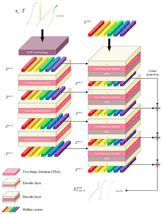
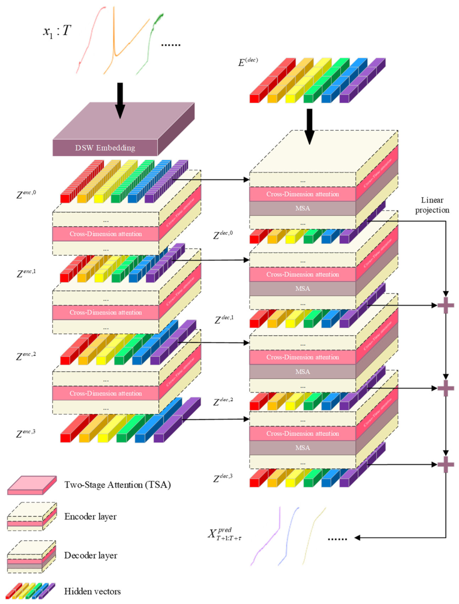
The Crossformer model, a Transformer-based architecture for multivariate time series forecasting, could be modified and employed to predict future discharge, precipitation, and water levels using historical data. As shown in Figure 4, the model comprises data processing layers, embedding layers, attention layers, encoding layers, and decoding layers.
Figure 4.
Crossformer model structure.
The simulation-based dataset used for Crossformer model development comprised 14,256 time-step records organized into 33 condition-specific sequences, each containing 432 ordered steps. Each record contained six variables: discharge, precipitation, and four water-depth variables (depth1–depth4). Each forecast sample consisted of 64 consecutive input steps and the subsequent four target steps. Sliding windows were constructed with a stride of one, yielding 365 samples per condition. Overlapping forecast windows are distinguished from time-step records and do not represent independent flood events. An additional observed flood event, 20230822, was retained as a separate external evaluation dataset. The event was held out in its entirety and was not used for Crossformer training, fitting standardization parameters, hyperparameter selection, early stopping, or selecting a model from repeated runs.
Before standardization and window construction, the complete simulated conditions were randomly assigned to training, validation, and test subsets using a fixed split seed of 42. The subsets contained 23, 3, and 7 conditions, respectively, corresponding to approximately 70%, 10%, and 20% of the simulated conditions. The original temporal order was preserved within each condition; no condition was shared between subsets, and no input–target window crossed a condition boundary. This yielded 8395 training, 1095 validation, and 2555 test samples. Condition-level partitioning was chosen to evaluate forecasts for simulated conditions withheld from training while retaining the temporal structure of each sequence. The same partition was used across repeated training runs. Hyperparameter selection, early stopping, and checkpoint selection used the validation subset, whereas the simulated test subset was reserved for final evaluation.
Feature-wise z-score standardization was applied before window construction:
where (μj,tr) and (σj,tr) are the mean and population standard deviation calculated exclusively from the 9936 original training records. Zero standard deviations were replaced by one. The saved parameters were applied unchanged to all subsets.
The embedding layer restructures the data using the Dimension-Segment-Wise (DSW) embedding method. With DSW, data from each dimension is divided into multiple segments of length Lseq. Each segment is mapped to a vector through linear projection and positional embedding, effectively capturing local patterns and intra-dimensional dependencies [19].
The self-attention layer processes the embedded data using the multi-head attention mechanism, where each head independently calculates and normalizes attention scores. To further enhance performance, Crossformer adopts a Two-Stage Attention (TSA) layer. First, the Cross-Time Stage applies the multi-head self-attention mechanism (MSA) to a 2D array Z, capturing dependencies between different temporal segments within each dimension [19]. Second, the Cross-Dimension Stage faces a challenge: direct application of MSA would result in a computational complexity of O(D2), which is unmanageable for large-scale datasets with high dimensionality D. To mitigate this, a router mechanism is introduced into Crossformer. A few learnable vectors (called routers) aggregate information from all dimensions at each timestep, then redistribute this aggregated information to establish full connectivity among dimensions. This mechanism reduces computational complexity to O(2cD) = O(D), significantly improving computational efficiency.
The encoding layer processes embeddings from the preceding layer using stacked scaling blocks. Each scaling block first merges adjacent segments through a segment merging layer, reducing the data scale while broadening feature representation. The merged data then enters the TSA layer, where multi-head attention mechanisms further analyze and refine the features. This process strengthens cross-dimensional correlations and enriches semantic context within the data [19].
The decoding layer employs a Hierarchical Encoder–Decoder (HED) structure to progressively process encoded data through multiple decoder layers. Each decoder layer uses self-attention and cross-attention mechanisms to enhance feature associations and integrate contextual information. The output of each layer contributes to the input of the next layer and the final prediction. This hierarchical processing improves data comprehension across layers [19]. Ultimately, the decoding layer aggregates predictions from all layers to form the forecasts for future discharge, precipitation, and water levels at different locations.
3.3.3. Model Evaluation Criteria
Model evaluation is a crucial step in assessing the effectiveness of feature selection methods [39]. To comprehensively evaluate the performance of feature selection models employed in regression problems, various statistical metrics are incorporated as evaluation criteria. Line graphs are plotted with the x-axis representing the validation set samples and the y-axis representing their values. Additionally, the metric definitions, evaluation scale, and unit conventions are summarized in Table S1. The evaluation parameters used in this study include the coefficient of determination (R2 score), mean squared error (MSE), mean absolute error (MAE), root mean squared error (RMSE), mean absolute percentage error (MAPE), and mean squared percentage error (MSPE).
3.3.4. Model Optimization
Overfitting represents a fundamental challenge in deep learning applications, occurring when a model fits excessively closely to the training data and consequently compromises its predictive accuracy on unseen data [40]. To mitigate overfitting during model development, Early Stopping—a regularization technique that halts training when validation performance plateaus—is employed to prevent excessive adaptation to training noise [41,42]. Additionally, Bayesian optimization is also utilized to identify optimal hyperparameter configurations, enhancing operational efficiency while navigating high-dimensional parameter spaces [43].
Early Stopping
The loss on the validation set is monitored over consecutive epochs. Continue training if the validation loss Lp satisfies the following condition over consecutive p (patience), as in Equation (15):
where Lv represents the current epoch’s validation loss, Lmin is the best validation loss from previous epochs, and δ is a positive value representing the minimum considered significant improvement in loss. If this condition is met within the specified p epochs, it is assumed that the model has stabilized, and further training would lead to overfitting. When triggered, the best-performing model state (achieving the lowest validation loss) is saved [44].
Lv < Lmin+δ
Bayesian Optimization
Bayesian optimization could efficiently explore high-dimensional hyperparameter spaces to maximize evaluation (e.g., R2). As an efficient global optimization strategy, it is particularly valuable for tuning machine learning models and optimizing functions with high evaluation costs [45]. The negative coefficient of determination (− R2) serves as the optimization target. A Gaussian process (GP) establishes the prior about the objective function, formalized as Equation (16):
where m(x) is the mean function, typically assumed to be zero, and k(x, x′) is the covariance function, representing the correlation between input points x and x′.
f(x)~(m(x),k(x, x′))
After each simulation, the GP posterior distribution is updated based on simulation results.
Posterior mean:
Posterior variance:
where X is the collection of all observation points, y is the corresponding observed values, K is the covariance matrix, is the noise variance, and I is the identity matrix.
The Expected Improvement (EI) acquisition function is used to explore regions minimizing −R2, as shown in Equation (19):
where f(x+) is the current maximum observed value.
EI(x) = 𝔼[max(f(x) − f(x+),0)]
The estimates of parameter effects are finely tuned in this process, guiding subsequent parameter selection. Through cyclic refinement, combinations of parameters yielding the worst model performance are systematically identified, elucidating specific parameter impacts on model behavior [46].
4. Results and Discussion
4.1. Relationship Analysis of Discharge, Precipitation and Water Level
Spearman rank correlation and Dynamic Time Warping (DTW) analyses were conducted on discharge, precipitation, and water levels at four locations (WL-2, WLGS-3, WLGS-4, WLGS-5) to assess the correlations and relationships in terms of overall patterns and similarities among the data. The analysis used 14,256 records from 33 simulated conditions, each containing 432 ordered steps. All six series were analysed at a uniform 10-min resolution. Discharge denotes the prescribed upstream inflow hydrograph used to drive HEC-RAS (m3/s), while precipitation denotes the design-storm rainfall forcing series (mm per 10-min interval).
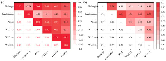
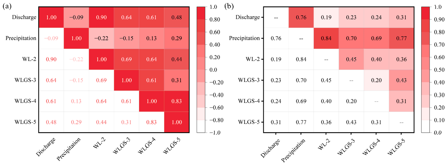
Spearman’s correlation matrix is presented in Figure 5a, analyzing the correlations between these variables. Values range from −1 to 1, with colors from light to dark representing the strength of the correlations [47]. Red indicated a positive correlation, while lighter colors denoted negative or non-significant correlations. Discharge showed strong positive correlations with all water levels, especially with WL-2 (r = 0.90), indicating the closest relationship. In contrast, the correlation between discharge and precipitation was weak (r = −0.09), suggesting no significant correlation. Precipitation also had a low correlation with the water levels, notably a negative correlation with WL-2 (r = −0.22), implying minimal influence at this site. Additionally, WLGS-5 and WLGS-4 demonstrated the strongest correlation (r = 0.83), indicating high consistency in their changes in water level. In summary, discharge is significantly positively correlated with the water levels (especially WL-2), while precipitation shows weak correlations, even negative ones at WL-2. Water-level changes between WLGS-5 and WLGS-4 are highly consistent.
Figure 5.
(a) Spearman’s correlation analysis matrix, (b) dynamic time warping analysis matrix.
Dynamic Time Warping (DTW) analysis was used to compare the overall shape and similarity of time series [48]. The DTW matrix (Figure 5b) displays the matching distance between variables after time alignment, where smaller values indicate higher shape similarity and larger values indicate greater differences. The color intensity (light to dark) corresponds to the magnitude of the matching distance.
The analysis shows that the smallest median DTW distance occurred between discharge and WL-2 (0.194), followed by WLGS-3 and WLGS-4 (0.198). Discharge also exhibited relatively small distances with WLGS-3, WLGS-4, and WLGS-5, at 0.232, 0.240, and 0.308, respectively. Among the water-depth pairs, the largest median distance occurred between WL-2 and WLGS-3 (0.454). Precipitation had larger distances with the other five series, ranging from 0.691 to 0.836, reflecting its distinct temporal pattern. Overall, the DTW distances indicate greater temporal similarity between discharge and water depth than between precipitation and water depth, with the water-depth series at different locations also showing relatively high temporal similarity.
Overall, discharge showed positive associations with the four water-depth series, with the strongest association and greatest temporal similarity at WL-2. The water-depth series also exhibited relatively high temporal similarity across locations, while precipitation showed a distinct temporal pattern. These findings provide a rationale for the joint multivariate forecasting approach adopted in this study.
4.2. Hydrologic and Hydraulic Modeling Analysis
To comprehensively assess the hydrological and hydraulic characteristics of the study area, hydrological and hydraulic simulations were conducted applying HEC-HMS and HEC-RAS, respectively. The HEC-HMS hydrological model is used for simulating the rainfall–runoff process at the sub-watershed scale, while the HEC-RAS model is utilized for river hydraulics simulation.
To ensure the accuracy of the hydrological simulation, initial HEC-HMS parameter values were estimated from engineering records, terrain data, land-cover information, and soil characteristics. These estimates were subsequently refined using the SCE-UA global optimization algorithm, with the SCS curve number (CN), initial abstraction, impervious-area percentage, and SCS unit hydrograph lag time treated as optimization variables. Calibration was conducted against observed rainfall–runoff data from 9 June 2022 by minimizing the RMSE between observed and simulated discharges. The resulting calibrated parameter values for the five subbasins are summarized in Table 2.
Table 2.
Final parameter values adopted for the HEC-HMS subbasins.
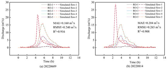
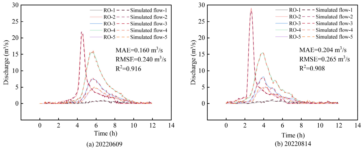
The calibrated model was subsequently validated using the rainfall–runoff event of 14 August 2022. Simulated discharges were compared with the corresponding observed records, and model performance was assessed using R2, MAE, and RMSE. Figure 6a,b present the discharge comparisons for the calibration and validation events, respectively. RO-1 to RO-5 denote the observed discharge series at the five comparison locations, while Simulated flow-1 to Simulated flow-5 denote the corresponding simulated discharge series. These comparisons provide a quantitative assessment of the hydrological simulations used in the subsequent HEC-RAS hydraulic modelling.
Figure 6.
Comparison of runoff gauging station data with HEC-HMS runoff modeling data for two events: (a) 20220609, (b) 20220814.
As shown in Figure 6a,b, the simulated discharges align well with the observed data from the five stations, accurately capturing the timing of peak flows and reflecting major trends and variations, particularly in the timing of flow events. The peak runoff in Figure 6b occurred earlier than in Figure 6a, potentially due to differences in precipitation intensity. Additionally, the peak runoff at RO-2 occurred earliest, while peak runoffs at other stations occurred at roughly the same time, which could be attributed to the hydrological characteristics of the sub-basins. Quantitative evaluation yielded R2 values of 0.916 and 0.908, MAE values of 0.160 and 0.204 m3/s, and RMSE values of 0.240 and 0.265 m3/s for the two events, respectively, further supporting the agreement between observed and simulated discharge.
Overall, the HEC-HMS model performed well in predicting flow events. The hydrological model was then used to simulate rainfall–runoff for different recurrence intervals, and the simulation results were utilized for river hydraulic simulations in HEC-RAS.
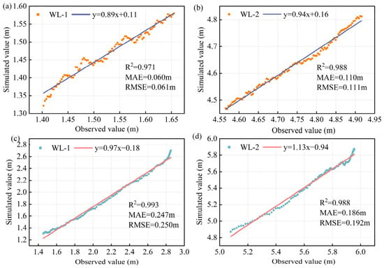
Given the limited availability of monitored rainstorm events and associated hydrological observations, HEC-RAS was calibrated using observations from an event with relatively low rainfall (20230928) and validated against observations from a more intense rainstorm (20220625). Observed discharge hydrographs were supplied as flow inputs. Calibration focused on Manning’s roughness coefficients, which were iteratively adjusted by comparing simulated and observed water-level hydrographs at WL-1 and WL-2. The adopted coefficients were 0.027 for the main channel, 0.015 for both bank slopes, and 0.035 for the left and right overbank areas, as summarized in Table 3. Figure 7 presents 100 paired observed and simulated water-level records for each station during calibration (Figure 7a,b) and validation (Figure 7c,d).
Table 3.
Manning’s roughness coefficients adopted for different hydraulic zones.
Figure 7.
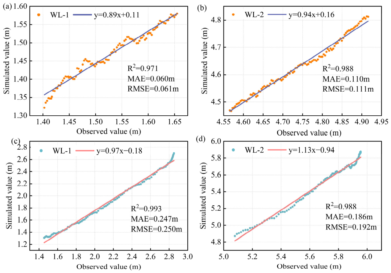
Comparison of HEC-RAS model calibration and validation for water levels at WL-1 and WL-2 stations: (a) WL-1 calibration; (b) WL-2 calibration; (c) WL-1 validation; (d) WL-2 validation.
Figure 7a shows a close linear relationship between observed and simulated water levels, with a fitted slope of 0.89 and an intercept of 0.11, indicating slight underestimation at WL-1. In Figure 7b, the WL-2 data are closely distributed around the fitted line with a slope of 0.94. During validation, strong linear correspondence remained at WL-1 (slope = 0.97; Figure 7c), with some deviations at higher water levels. The WL-2 data also closely followed the fitted line (slope = 1.13; Figure 7d), although the fitted relationship indicated underestimation over the observed water-level range. Quantitatively, calibration MAE and RMSE were 0.060–0.110 m and 0.061–0.111 m, respectively, while validation MAE and RMSE were 0.186–0.247 m and 0.192–0.250 m. The observed–simulated regression R2 ranged from 0.971 to 0.993 across the four comparisons. The larger validation errors may partly reflect the limited representation of high-flow conditions during calibration. Nevertheless, the strong observed–simulated correspondence indicates that HEC-RAS reproduced the main water-level variations. Together, the graphical comparisons and quantitative metrics support the use of the calibrated model to construct the simulation-based Crossformer dataset for the evaluated river reach and conditions.
4.3. Crossformer Performance
A comprehensive simulation process was investigated to evaluate the performance of the Crossformer model in a hydrological simulation task. The hyperparameters of the model were first optimized using a Bayesian method. The hyperparameter space is defined in Table 4. By constructing a target function that calculates the model’s R2 score for each hyperparameter set and minimizes the -R2, the optimization process aimed to maximize model performance.
Table 4.
Hyperparameters, search space, and search results for Bayesian optimization.
After 50 calls, Bayesian optimization provided an optimal set of hyperparameters, which significantly improved the prediction accuracy of the model. Under the optimal settings, ten parallel simulations were performed, and the corresponding evaluation metrics are listed in Table 5. The R2 scores ranged from 0.968 to 0.975, with an average of 0.970, indicating that the model can explain approximately 97% of the data variance. MSE and MAE ranged between 0.014 and 0.019 and 0.034 and 0.050, respectively, with averages of 0.017 and 0.043, demonstrating high and stable prediction accuracy. The average RMSE was 0.132, higher than the MAE, yet still denoting satisfactory performance. MAPE ranged from 0.092 to 0.156 with an average of 0.119, showing minor predictive errors. Although the MSPE showed considerable variation (2.189 to 22.560) with an average of 7.949, this occurred only under specific conditions. The results show that the Bayesian-optimized Crossformer model generally proved accurate and suitable for predictive tasks.
Table 5.
Evaluation results of ten parallel simulations with optimal parameters.
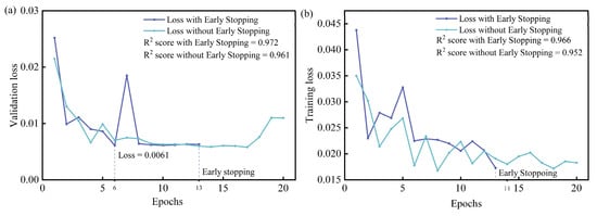
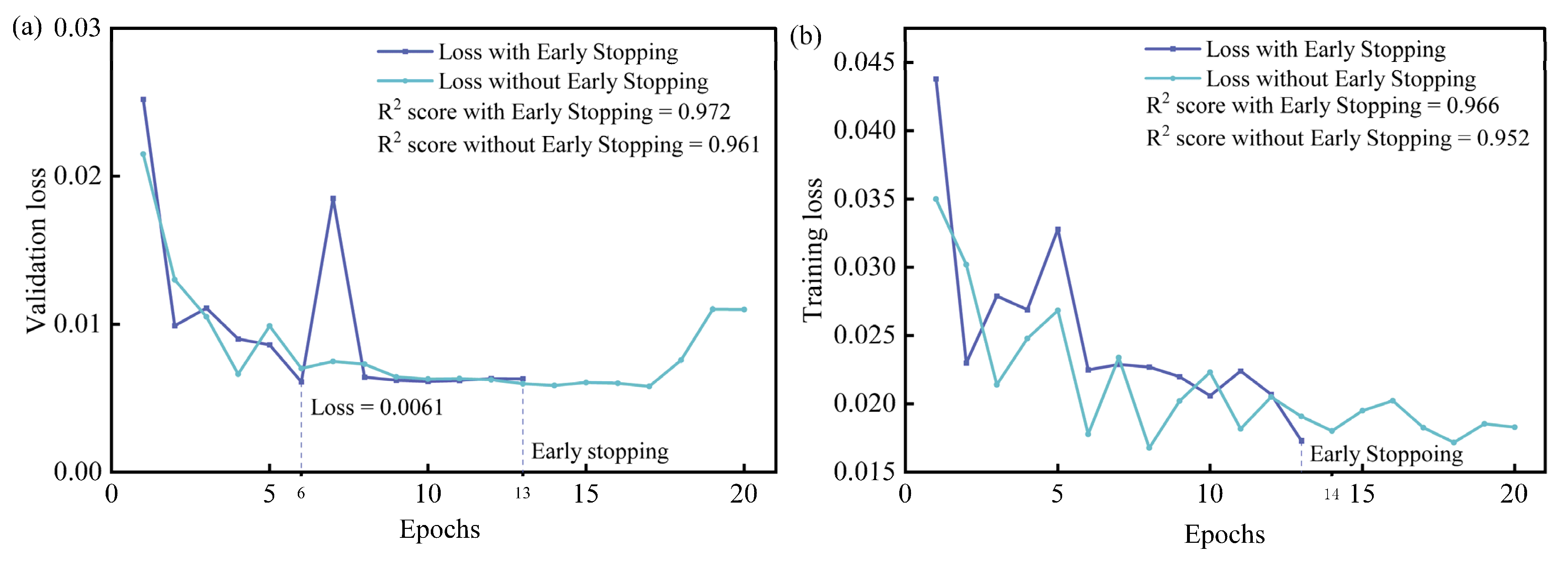
The use of Early Stopping helped prevent overfitting while maintaining the generalization ability of the model. As illustrated in Figure 8a, training with Early Stopping resulted in the lowest loss at the 6th epoch (0.0061). Validation loss exceeded 0.0061 after 7 cycles, triggering Early Stopping at the 13th cycle, thus maintaining the optimal status and preventing overfitting. In contrast, the model without Early Stopping exhibited a final Loss value of 0.0101 and showed greater fluctuation in training loss (Figure 8b), indicating potential overfitting. The higher R2 score further confirms that Early Stopping improved model stability and efficiency, validating the model having higher explanatory power [49].
Figure 8.
Comparative chart of trends in losses with or without Early Stopping. (a) Trend of loss with increasing number of iterations on the validation dataset. (b) Trend of loss with increasing number of iterations on the Training dataset.
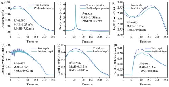
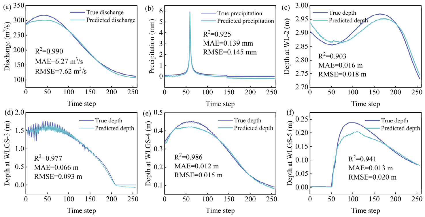
Finally, the trained Crossformer model was evaluated on the independently held-out observed flood event identified as 20230822. This event was not used for the calibration or validation of either HEC-HMS or HEC-RAS. It was also excluded from Crossformer training, fitting standardization parameters, hyperparameter selection, early stopping, and model selection. The predictions were compared with the corresponding field observations, as shown in Figure 9. This external observed-event evaluation was reported separately from the internal test using simulation-based reference data. The Crossformer model generally captured the observed temporal variations in discharge, precipitation, and water depth. Flow predictions (Figure 9a) closely matched observed values, with an R2 of 0.990, an MAE of 6.27 m3/s, and an RMSE of 7.62 m3/s, indicating good agreement throughout the flood process. Although rainfall predictions (Figure 9b) were slightly lower in the later stages, the overall trend remains consistent with measurements, yielding an R2 of 0.925, an MAE of 0.139 mm, and an RMSE of 0.145 mm. Water depth predictions (Figure 9c–f) also performed well, especially in simulating the peak water depth and its subsequent decline, although slight deviations in peak timing and precision occurred in Figure 9e,f. Across these locations, R2 ranged from 0.903 to 0.986, MAE from 0.012 to 0.066 m, and RMSE from 0.015 to 0.093 m. Overall, the model reproduced the main temporal variations in discharge, precipitation, and water depth during the evaluated flood event. These results provide independent observational support for the predictive performance of the proposed simulation-assisted multivariate forecasting framework.
Figure 9.
True values vs. predicted values of Crossformer. (a) Discharge; (b) precipitation; (c) depth at WL-2; (d) depth at WLGS-3; (e) depth at WLGS-4; (f) depth at WLGS-5.
Notably, both models were evaluated under the same hardware and computational conditions. The average prediction time of Crossformer was 7.13 s, compared with 15.2 min for HEC-RAS simulation, corresponding to an execution-time ratio of approximately 128. These timings excluded model training and input preprocessing and indicate a computational advantage during the timed prediction and simulation stages. These results indicate a computational advantage for Crossformer in the evaluated task, supporting its potential for rapid flood prediction.
4.4. Crossformer Model Analysis
The local sensitivity of hyperparameters and performance of the Crossformer model under data uncertainty are the primary concerns of the analysis. Local sensitivity to hyperparameters was assessed by examining the variations in hyperparameter settings on the model performance metrics such as R2 scores. This enables the identification of the most influential hyperparameters, thereby guiding more effective tuning strategies [50]. To assess robustness against data uncertainty, Gaussian noise was introduced into the dataset to simulate real-world unpredictability. Changes in performance metrics, including MSE and MAE, were subsequently analyzed to evaluate the model performance of maintaining accuracy and reliability under noisy conditions [51].
Experiments with different hyperparameter configurations revealed that model dimension and learning rate significantly influence model performance. As shown in Table 6, increasing the model dimension from 256 to 1024 resulted in a significant improvement in R2 value from 0.836 to 0.917. This indicated that model performance could be enhanced by larger model dimensions. Furthermore, an optimal learning rate (3.9 × 10⁻⁵) yielded the highest R2 score (0.915), while deviations from the learning rate both led to decreased performance. This underscores the importance of selecting an appropriate learning rate to balance learning speed and model convergence, a critical factor in optimization [52].
Table 6.
Mean and standard deviation of R2 score at different hyperparameter values.
To simulate data variability and uncertainty, Gaussian noise was randomly added to the dataset [53]. Gaussian input perturbations were evaluated using a fixed Crossformer checkpoint and unchanged reference targets. Noise was added to all six standardized input variables at σ = 0.05, 0.10, 0.20 and 0.30, with ten realizations per level using seeds 2026–2035. Standardization parameters were fitted exclusively to the training data, and no retraining was performed. Each noise level was compared with the noise-free baseline obtained from the same checkpoint. As shown in Table 7, Crossformer retained high pooled R2 values under the evaluated Gaussian input perturbations. At σ = 0.05, the increase in prediction errors was relatively small, suggesting potential applicability to hydrological prediction under mild input uncertainty. Larger perturbations caused more pronounced degradation in predictive accuracy.
Table 7.
Performance of the Crossformer model using datasets with different Gaussian noises added.
In summary, local sensitivity analysis revealed that model dimension and learning rate were key hyperparameters influencing the Crossformer performance. The model also maintained good predictive performance under low levels of Gaussian input noise. These findings provide strong support for further optimization and application of the Crossformer model, ensuring its effectiveness and reliability in hydrological modeling scenarios.
5. Conclusions
To address the scarcity of precipitation data, this study developed a novel framework integrating HEC-HMS, HEC-RAS, and Crossformer for river-flood prediction. The main conclusions are as follows:
- (1)
- HEC-HMS and HEC-RAS reproduced the main observed discharge and water-level variations for the studied reach. HEC-HMS yielded R2 values of 0.916 and 0.908, with RMSE values of 0.240 and 0.265 m3/s for the two evaluated events. HEC-RAS water-level RMSE ranged from 0.061 to 0.111 m during calibration and from 0.192 to 0.250 m during validation.
- (2)
- Crossformer achieved consistent predictive performance on the held-out simulated conditions across ten runs, with R2 ranging from 0.968 to 0.975 and averaging 0.970. Mean MAE and RMSE were 0.043 and 0.132, respectively, on the standardized scale. These results demonstrate its ability to reproduce the multivariate responses represented in the simulation-based test dataset.
- (3)
- Evaluation on an independently held-out observed flood event showed that Crossformer generally reproduced the temporal variations in all six variables, including discharge, precipitation, and four water-depth series. Under the same hardware and computational conditions, the average Crossformer prediction time was 7.13 s, compared with 15.2 min for HEC-RAS simulation, corresponding to an approximately 128-fold computational speedup.
- (4)
- Predictive performance depended on model configuration and input perturbation magnitude. In the tested configurations, increasing the hidden-state dimension from 256 to 1024 raised mean R2 from 0.836 to 0.917. With a fixed trained model, Gaussian input perturbations at σ = 0.05 reduced pooled R2 from 0.970 to 0.967, whereas σ = 0.30 reduced it to 0.914 and increased standardized MAE from 0.043 to 0.164. Thus, mild perturbations produced relatively small accuracy losses, while stronger perturbations caused progressively larger prediction errors.
In summary, integrating existing data with hydrological models and Crossformer provides an approach to data supplementation and prediction under limited observations, with potential to support flood early-warning and mitigation decisions. Crossformer’s evaluation against field observations was limited to a single flood event owing to the scarcity of available monitoring data. Future work will incorporate more high-quality rainfall, discharge, and water-level observations for model training, validation, and optimization, and assess its potential for real-time flood forecasting across multiple independent events.
Supplementary Materials
The following supporting information can be downloaded at https://www.mdpi.com/article/10.3390/w18212678/s1. Figure S1: Location of study area. Figure S2: Chicago design hyetographs for different return periods. Figure S3: Spatial input data. (a) Land cover (from 1985–2022 China 30-m annual land cover dataset and its dynamics, sourced from zenodo.org), (b) soil classification (from the Harmonized World Soil Database v1.2 available on the FAO Soil Portal website). Table S1: Statistical criteria for evaluation. Data: The complete simulation-based dataset.
Author Contributions
Conceptualization, H.L.; methodology, Y.L., F.L., H.Z. and H.L.; software, Y.L. and F.L.; validation, Y.L., S.D., H.L. and M.L.; formal analysis, F.L.; investigation, H.Z., Y.C. and L.W.; resources, S.D.; data curation, Y.C. and L.W.; writing—original draft preparation, F.L.; writing—review and editing, Y.L., S.D., H.L. and M.L.; supervision, S.D., H.L. and M.L.; funding acquisition, M.L. All authors have read and agreed to the published version of the manuscript.
Funding
This research was funded by the Shandong Province Program for Enhancing the Innovation Capabilities of Science and Technology-Based Small and Medium-Sized Enterprises, grant number 2024TSGC0230; the Qingdao Municipal Science and Technology Bureau, grant number 25-1-1-yqpy-10-qy; the Natural Science Foundation of Shandong Province, grant number ZR2026QC0540; and the National Natural Science Foundation of China, grant number 51708312.
Data Availability Statement
The simulation-based dataset is provided in the Supplementary Materials. The observed hydrological records and engineering data are subject to proprietary and contractual restrictions and may be made available upon reasonable request, subject to permission from the project owner.
Acknowledgments
Regarding the use of generative artificial intelligence, ChatGPT (GPT-6.1 Sol, OpenAI) was used only for proofreading and text-editing purposes, such as checking grammar, spelling, punctuation, formatting, and textual consistency. It was not used to generate scientific content, data, graphics, or study design, or for data collection, data analysis, or the interpretation of results.
Conflicts of Interest
Authors Yunpeng Chen and Luohua Wang were employed by Qingdao Yanboot Data Information Technology Co., Ltd. The remaining authors declare that the research was conducted in the absence of any commercial or financial relationships that could be construed as a potential conflict of interest.
Abbreviations
The following abbreviations are used in this manuscript:
| 1D | One-dimensional |
| 2D | Two-dimensional |
| ANN | Artificial neural network |
| CN | Curve number |
| CNN | Convolutional neural network |
| DEM | Digital elevation model |
| DSW | Dimension-segment-wise embedding |
| DTW | Dynamic time warping |
| EI | Expected improvement |
| FFN | Feed-forward network |
| GP | Gaussian process |
| HED | Hierarchical encoder–decoder |
| IDF | Intensity–duration–frequency |
| LSTM | Long short-term memory |
| MAE | Mean absolute error |
| MAPE | Mean absolute percentage error |
| ML | Machine learning |
| MLP | Multilayer perceptron |
| MSA | Multi-head self-attention |
| MSE | Mean squared error |
| MSPE | Mean squared percentage error |
| PE | Positional encoding |
| ReLU | Rectified linear unit |
| RMSE | Root mean squared error |
| SCS-CN | Soil Conservation Service curve number |
| SD | Standard deviation |
| TSA | Two-stage attention |
| USACE | United States Army Corps of Engineers |
References
- Teng, J.; Jakeman, A.J.; Vaze, J.; Croke, B.F.W.; Dutta, D.; Kim, S. Flood Inundation Modelling: A Review of Methods, Recent Advances and Uncertainty Analysis. Environ. Model. Softw. 2017, 90, 201–216. [Google Scholar] [CrossRef] [Scilit]
- Sauer, I.J.; Mester, B.; Frieler, K.; Zimmermann, S.; Schewe, J.; Otto, C. Limited Progress in Global Reduction of Vulnerability to Flood Impacts over the Past Two Decades. Commun. Earth Environ. 2024, 5, 239. [Google Scholar] [CrossRef] [Scilit]
- Grant, L.; Vanderkelen, I.; Gudmundsson, L.; Fischer, E.; Seneviratne, S.I.; Thiery, W. Global Emergence of Unprecedented Lifetime Exposure to Climate Extremes. Nature 2025, 641, 374–379. [Google Scholar] [CrossRef] [Scilit] [PubMed]
- Yin, Z.; Hu, Y.; Jenkins, K.; He, Y.; Forstenhäusler, N.; Warren, R.; Yang, L.; Jenkins, R.; Guan, D. Assessing the Economic Impacts of Future Fluvial Flooding in Six Countries under Climate Change and Socio-Economic Development. Clim. Change 2021, 166, 38. [Google Scholar] [CrossRef] [Scilit]
- Jongman, B.; Winsemius, H.C.; Aerts, J.C.J.H.; Coughlan De Perez, E.; Van Aalst, M.K.; Kron, W.; Ward, P.J. Declining Vulnerability to River Floods and the Global Benefits of Adaptation. Proc. Natl. Acad. Sci. USA 2015, 112, E2271–E2280. [Google Scholar] [CrossRef] [Scilit] [PubMed]
- Nearing, G.; Cohen, D.; Dube, V.; Gauch, M.; Gilon, O.; Harrigan, S.; Hassidim, A.; Klotz, D.; Kratzert, F.; Metzger, A.; et al. Global Prediction of Extreme Floods in Ungauged Watersheds. Nature 2024, 627, 559–563. [Google Scholar] [CrossRef] [Scilit] [PubMed]
- Pirone, D.; Padulano, R.; Del Giudice, G. Approaching Urban Flood Modelling According to Available Data: A State-of-the-Art Review and Future Challenges. J. Flood Risk Manag. 2026, 19, e70184. [Google Scholar] [CrossRef] [Scilit]
- Piadeh, F.; Behzadian, K.; Alani, A.M. A Critical Review of Real-Time Modelling of Flood Forecasting in Urban Drainage Systems. J. Hydrol. 2022, 607, 127476. [Google Scholar] [CrossRef] [Scilit]
- Duangkhwan, W.; Ekkawatpanit, C.; Petpongpan, C.; Kositgittiwong, D.; Kazama, S.; Hiraga, Y.; Jaturapitakkul, C. Enhancing Flood Forecasting with Deep Learning: A Scalable Alternative to Traditional Hydrodynamic Models. Environ. Model. Softw. 2026, 197, 106841. [Google Scholar] [CrossRef] [Scilit]
- Du, H.; Fei, K.; Wu, J.; Gao, L. An Integrative Modelling Framework for Predicting the Compound Flood Hazards Induced by Tropical Cyclones in an Estuarine Area. Environ. Model. Softw. 2024, 175, 105996. [Google Scholar] [CrossRef] [Scilit]
- Zeng, B.; Huang, G.; Chen, W. Research Progress and Prospects of Urban Flooding Simulation: From Traditional Numerical Models to Deep Learning Approaches. Environ. Model. Softw. 2025, 183, 106213. [Google Scholar] [CrossRef] [Scilit]
- Huynh, N.N.T.; Garambois, P.-A.; Renard, B.; Colleoni, F.; Monnier, J.; Roux, H. A Distributed Hybrid Physics–AI Framework for Learning Corrections of Internal Hydrological Fluxes and Enhancing High-Resolution Regionalized Flood Modeling. Hydrol. Earth Syst. Sci. 2025, 29, 3589–3613. [Google Scholar] [CrossRef] [Scilit]
- Chen, T.; Tian, J.; Sun, J.; Zhang, Z.; Chai, H.; Lin, B.; Fu, X. FloodUnet: A Rapid Spatio-Temporal Prediction Model for Flood Evolution Based on an Enhanced U-Net. Water Resour. Res. 2026, 62, e2025WR041427. [Google Scholar] [CrossRef] [Scilit]
- Li, W.; Liu, C.; Xu, Y.; Niu, C.; Li, R.; Li, M.; Hu, C.; Tian, L. An Interpretable Hybrid Deep Learning Model for Flood Forecasting Based on Transformer and LSTM. J. Hydrol. Reg. Stud. 2024, 54, 101873. [Google Scholar] [CrossRef] [Scilit]
- Castangia, M.; Grajales, L.M.M.; Aliberti, A.; Rossi, C.; Macii, A.; Macii, E.; Patti, E. Transformer Neural Networks for Interpretable Flood Forecasting. Environ. Model. Softw. 2023, 160, 105581. [Google Scholar] [CrossRef] [Scilit]
- Long, T.; Akbari, M.; Fakharian, P. Prediction of Soil Liquefaction Using a Multi-Algorithm Technique: Stacking Ensemble Techniques and Bayesian Optimization. J. Soft Comput. Civ. Eng. 2025, 9, 32–55. [Google Scholar] [CrossRef]
- Situ, Z.; Wang, Q.; Teng, S.; Feng, W.; Chen, G.; Zhou, Q.; Fu, G. Improving Urban Flood Prediction Using LSTM-DeepLabv3+ and Bayesian Optimization with Spatiotemporal Feature Fusion. J. Hydrol. 2024, 630, 130743. [Google Scholar] [CrossRef] [Scilit]
- Zhu, F.; Zhu, O.; Han, M.; Liu, W.; Guo, X.; Hou, T.; Zhao, L.; Xu, C.; Zhong, P. A Hybrid Process-Data Driven Framework for Real-Time Hydrological Forecasting with Interpretable Deep Learning. J. Hydrol. 2025, 662, 134082. [Google Scholar] [CrossRef] [Scilit]
- Zhang, Y.; Yan, J. Crossformer: Transformer Utilizing Cross-Dimension Dependency for Multivariate Time Series Forecasting. In Proceedings of the Eleventh International Conference on Learning Representations, Kigali, Rwanda, 1–5 May 2023. [Google Scholar]
- Haces-Garcia, F.; Ross, N.; Glennie, C.L.; Rifai, H.S.; Hoskere, V.; Ekhtari, N. Rapid 2D Hydrodynamic Flood Modeling Using Deep Learning Surrogates. J. Hydrol. 2025, 651, 132561. [Google Scholar] [CrossRef] [Scilit]
- Wang, S.; Xiang, Z.; Song, Y.; Wang, K.; Nian, X.; Feng, L.; Wang, J.; Xin, K.; Yan, H.; Tao, T. Real-Time Dynamic Urban Flood Prediction: An Integrated Deep Learning Architecture with Adaptive Updating. ACS EST Water 2026, 6, 3493–3509. [Google Scholar] [CrossRef] [Scilit]
- Tegegne, G.; Park, D.K.; Kim, Y.-O. Comparison of Hydrological Models for the Assessment of Water Resources in a Data-Scarce Region, the Upper Blue Nile River Basin. J. Hydrol. Reg. Stud. 2017, 14, 49–66. [Google Scholar] [CrossRef] [Scilit]
- Singh, V.P. Hydrologic Modeling: Progress and Future Directions. Geosci. Lett. 2018, 5, 15. [Google Scholar] [CrossRef] [Scilit]
- Ghoraba, S.M. Hydrological Modeling of the Simly Dam Watershed (Pakistan) Using GIS and SWAT Model. Alex. Eng. J. 2015, 54, 583–594. [Google Scholar] [CrossRef] [Scilit]
- Zhao, G.; Gao, H.; Naz, B.S.; Kao, S.-C.; Voisin, N. Integrating a Reservoir Regulation Scheme into a Spatially Distributed Hydrological Model. Adv. Water Resour. 2016, 98, 16–31. [Google Scholar] [CrossRef] [Scilit]
- Tibangayuka, N.; Mulungu, D.M.M.; Izdori, F. Evaluating the Performance of HBV, HEC-HMS and ANN Models in Simulating Streamflow for a Data Scarce High-Humid Tropical Catchment in Tanzania. Hydrol. Sci. J. 2022, 67, 2191–2204. [Google Scholar] [CrossRef] [Scilit]
- Bai, Y.; Zhang, Z.; Zhao, W. Assessing the Impact of Climate Change on Flood Events Using HEC-HMS and CMIP5. Water. Air. Soil Pollut. 2019, 230, 119. [Google Scholar] [CrossRef] [Scilit]
- Gumindoga, W.; Rwasoka, D.T.; Nhapi, I.; Dube, T. Ungauged Runoff Simulation in Upper Manyame Catchment, Zimbabwe: Application of the HEC-HMS Model. Phys. Chem. Earth Parts ABC 2017, 100, 371–382. [Google Scholar] [CrossRef] [Scilit]
- Hosseinzadeh-Tabrizi, A.; Ghaeini-Hessaroeyeh, M. Coupled Dam-Break Flow and Bed Load Modelling Using HLLC-WAF Scheme. Water Sci. Technol. 2015, 72, 1155–1167. [Google Scholar] [CrossRef] [Scilit] [PubMed]
- Vojtek, M.; Petroselli, A.; Vojteková, J.; Asgharinia, S. Flood Inundation Mapping in Small and Ungauged Basins: Sensitivity Analysis Using the EBA4SUB and HEC-RAS Modeling Approach. Hydrol. Res. 2019, 50, 1002–1019. [Google Scholar] [CrossRef] [Scilit]
- ShahiriParsa, A.; Noori, M.; Heydari, M.; Rashidi, M. Floodplain Zoning Simulation by Using HEC-RAS and CCHE2D Models in the Sungai Maka River. Air Soil Water Res. 2016, 9, ASWR.S36089. [Google Scholar] [CrossRef] [Scilit]
- Haykin, S. Neural Networks Expand SP’s Horizons. IEEE Signal Process. Mag. 1996, 13, 24–49. [Google Scholar] [CrossRef]
- Su, H.; Wang, X.; Qin, Y. AGCNT: Adaptive Graph Convolutional Network for Transformer-Based Long Sequence Time-Series Forecasting. In Proceedings of the 30th ACM International Conference on Information & Knowledge Management; ACM: Gold Coast, QLD, Australia, 2021; pp. 3439–3442. [Google Scholar]
- Li, Y.; Wang, H.; Li, J.; Liu, C.; Tan, J. ACT: Adversarial Convolutional Transformer for Time Series Forecasting. In Proceedings of the 2022 International Joint Conference on Neural Networks (IJCNN); IEEE: Padua, Italy, 2022; pp. 1–8. [Google Scholar]
- Liu, C.; Liu, D.; Mu, L. Improved Transformer Model for Enhanced Monthly Streamflow Predictions of the Yangtze River. IEEE Access 2022, 10, 58240–58253. [Google Scholar] [CrossRef] [Scilit]
- Mayer, J.; Caglar, T.; Jochem, R. Transformer Networks for Univariate Time Series Prediction in Predictive Process Control. In Proceedings of the 2023 IEEE International Conference on Engineering, Technology and Innovation (ICE/ITMC); IEEE: Edinburgh, UK, 2023; pp. 1–6. [Google Scholar]
- Shi, J.; Jain, M.; Narasimhan, G. Time Series Forecasting (TSF) Using Various Deep Learning Models. arXiv 2022, arXiv:2204.11115. [Google Scholar] [CrossRef] [Scilit]
- Gupta, A.; Mehta, V. Time Series Based Predictive Model for Analysing the Health of Power Transformer. In Proceedings of the 2023 International Conference on Innovative Data Communication Technologies and Application (ICIDCA); IEEE: Uttarakhand, India, 2023; pp. 1006–1013. [Google Scholar]
- Qi, C.; Diao, J.; Qiu, L. On Estimating Model in Feature Selection With Cross-Validation. IEEE Access 2019, 7, 33454–33463. [Google Scholar] [CrossRef] [Scilit]
- Kadhim, Z.S.; Abdullah, H.S.; Ghathwan, K.I. Automatically Avoiding Overfitting in Deep Neural Networks by Using Hyper-Parameters Optimization Methods. Int. J. Online Biomed. Eng. IJOE 2023, 19, 146–162. [Google Scholar] [CrossRef] [Scilit]
- Fedorenko, Y.S.; Gapanyuk, Y.E.; Minakova, S.V. The Analysis of Regularization in Deep Neural Networks Using Metagraph Approach. In Advances in Neural Computation, Machine Learning, and Cognitive Research; Kryzhanovsky, B., Dunin-Barkowski, W., Redko, V., Eds.; Studies in Computational Intelligence; Springer International Publishing: Cham, Switzerland, 2018; Volume 736, pp. 3–8. [Google Scholar]
- Bisong, E. Regularization for Deep Learning. In Building Machine Learning and Deep Learning Models on Google Cloud Platform; Apress: Berkeley, CA, USA, 2019; pp. 415–421. [Google Scholar]
- Pan, Z.; Lu, W.; Fan, Y.; Li, J. Identification of Groundwater Contamination Sources and Hydraulic Parameters Based on Bayesian Regularization Deep Neural Network. Environ. Sci. Pollut. Res. 2021, 28, 16867–16879. [Google Scholar] [CrossRef] [Scilit] [PubMed]
- Perin, G.; Wu, L.; Picek, S. The Need for Speed: A Fast Guessing Entropy Calculation for Deep Learning-Based SCA. Algorithms 2023, 16, 127. [Google Scholar] [CrossRef] [Scilit]
- Klein, A.; Falkner, S.; Bartels, S.; Hennig, P.; Hutter, F. Fast Bayesian Hyperparameter Optimization on Large Datasets. Electron. J. Stat. 2017, 11, 4945–4968. [Google Scholar] [CrossRef] [Scilit]
- Polyzos, K.D.; Lu, Q.; Giannakis, G.B. Bayesian Optimization with Ensemble Learning Models and Adaptive Expected Improvement. In Proceedings of the ICASSP 2023—2023 IEEE International Conference on Acoustics, Speech and Signal Processing (ICASSP); IEEE: Rhodes Island, Greece, 2023; pp. 1–5. [Google Scholar]
- Puth, M.-T.; Neuhäuser, M.; Ruxton, G.D. Effective Use of Spearman’s and Kendall’s Correlation Coefficients for Association between Two Measured Traits. Anim. Behav. 2015, 102, 77–84. [Google Scholar] [CrossRef] [Scilit]
- Wan, X.; Li, H.; Zhang, L.; Wu, Y.J. Multivariate Time Series Data Clustering Method Based on Dynamic Time Warping and Affinity Propagation. Wirel. Commun. Mob. Comput. 2021, 2021, 9915315. [Google Scholar] [CrossRef] [Scilit]
- Ying, X. An Overview of Overfitting and Its Solutions. J. Phys. Conf. Ser. 2019, 1168, 022022. [Google Scholar] [CrossRef] [Scilit]
- Probst, P.; Wright, M.N.; Boulesteix, A. Hyperparameters and Tuning Strategies for Random Forest. WIREs Data Min. Knowl. Discov. 2019, 9, e1301. [Google Scholar] [CrossRef] [Scilit]
- Guo, C.; Song, B.; Wang, Y.; Chen, H.; Xiong, H. Robust Variable Selection and Estimation Based on Kernel Modal Regression. Entropy 2019, 21, 403. [Google Scholar] [CrossRef] [Scilit] [PubMed]
- Novello, P.; Poëtte, G.; Lugato, D.; Congedo, P.M. Goal-Oriented Sensitivity Analysis of Hyperparameters in Deep Learning. J. Sci. Comput. 2023, 94, 45. [Google Scholar] [CrossRef] [Scilit]
- Keshavarzzadeh, V.; Kirby, R.M.; Narayan, A. Stress-Based Topology Optimization under Uncertainty via Simulation-Based Gaussian Process. Comput. Methods Appl. Mech. Eng. 2020, 365, 112992. [Google Scholar] [CrossRef] [Scilit]

Disclaimer/Publisher’s Note: The statements, opinions and data contained in all publications are solely those of the individual author(s) and contributor(s) and not of MDPI and/or the editor(s). MDPI and/or the editor(s) disclaim responsibility for any injury to people or property resulting from any ideas, methods, instructions or products referred to in the content. |
© 2026 by the authors. Licensee MDPI, Basel, Switzerland. This article is an open access article distributed under the terms and conditions of the Creative Commons Attribution (CC BY) license.