


Abstract
Accurate long-range forecasting of sea surface temperature (SST) fields remains challenging because regional SST variability reflects the combined influence of recurrent seasonal behavior and shorter-term oceanographic processes. This study develops a forecasting framework combining Multivariate Singular Spectrum Analysis (MSSA) and Dynamic Mode Decomposition (DMD), hereafter referred to as MSSA-DMD, for daily SST forecasting in the Marmara Sea. The framework first represents the SST field in a reduced empirical orthogonal function (EOF) space, separates the temporal dynamics into reconstructed MSSA components, and independently propagates these components using DMD before reconstructing the full SST field. Daily Copernicus Marine Service SST data were evaluated for forecast horizons ranging from 1 to 60 days. The proposed approach was compared with Standard DMD, multivariate empirical mode decomposition (MEMD)–DMD, multivariate variational mode decomposition (MVMD)–DMD, direct inverted Transformer (iTransformer), MSSA-iTransformer, persistence, and climatology. MSSA-DMD provided the most consistent overall forecasting performance, with its advantage becoming particularly evident at extended lead times while maintaining stable spatial and temporal error characteristics. The improvement of MSSA-iTransformer over direct iTransformer further indicates that MSSA decomposition itself contributes substantially to predictive skill. Computational analysis additionally showed that MSSA-DMD achieved a considerably lower end-to-end execution cost than the iTransformer-based configurations. These findings demonstrate that decomposition-assisted reduced-order forecasting, particularly through MSSA-DMD, provides an effective accuracy–cost balance for long-range regional SST prediction.
1. Introduction
Sea surface temperature (SST) is a fundamental indicator of the thermal state of the upper ocean and a key variable governing interaction between the ocean and atmosphere. Variations in SST regulate exchanges of heat, moisture, and momentum across the air–sea interface and influence atmospheric circulation, upper-ocean stratification, marine ecosystems, fisheries, and coastal environmental conditions. SST anomalies are also closely associated with marine and atmospheric extremes, including marine heatwaves, tropical cyclones, storm-related coastal hazards, and persistent warming or cooling episodes [1,2,3]. Reliable prediction of SST is therefore important for operational oceanography, climate assessment, marine-hazard preparedness, ecosystem management, and the sustainable use of coastal and regional seas.
The evolution of SST is governed by the combined influence of solar radiation, turbulent air–sea heat exchange, wind forcing, surface and subsurface circulation, horizontal advection, vertical mixing, stratification, freshwater input, and exchanges with adjacent water masses. These mechanisms act over markedly different temporal and spatial scales. Long-term background variability and the dominant seasonal heating–cooling cycle coexist with intermediate-scale circulation changes, synoptic atmospheric disturbances, and short-lived localized thermal anomalies. The observed SST field consequently represents a superposition of processes having different characteristic timescales, amplitudes, persistence levels, and spatial signatures. This multiscale behavior makes SST forecasting inherently difficult, particularly when the objective is not the prediction of a single time series but the simultaneous prediction of an entire spatially distributed temperature field. The challenge becomes even greater in coastal and semi-enclosed basins, where restricted water exchange, irregular coastlines, bathymetric variability, strong stratification, and rapidly varying atmospheric forcing can produce pronounced spatial heterogeneity.
Physics-based ocean circulation models provide the conventional framework for predicting SST by numerically solving governing equations describing momentum, mass conservation, heat transport, turbulence, and air–sea interaction. Such models provide physically consistent representations of ocean dynamics and remain indispensable for operational forecasting. Their performance, however, depends strongly on the accuracy of atmospheric forcing, initial and boundary conditions, bathymetry, numerical resolution, and the parameterizations used to represent unresolved physical processes. Forecast uncertainty may therefore arise from errors in external forcing, limited spatial resolution, uncertain mixing formulations, and inadequately resolved coastal processes [3,4,5]. In addition, high-resolution numerical simulations may involve substantial computational requirements. The increasing availability of satellite observations, reanalysis products, and long-term gridded ocean datasets has consequently stimulated growing interest in data-driven alternatives that learn the temporal evolution of SST directly from historical observations.
A broad range of machine-learning and deep-learning approaches has been developed for this purpose. Early applications employed artificial neural networks and support vector regression for SST forecasting [6,7]. Subsequent studies introduced recurrent neural networks, including long short-term memory (LSTM) networks and gated recurrent units (GRUs), for modeling SST variability [8]. More recent studies have introduced convolutional recurrent architectures, attention mechanisms, Transformers, graph neural networks, U-Net variants, Mamba-based structures, and physics-guided neural networks [1,2,3,9,10,11,12,13,14,15,16,17]. Xiao et al. [1], for example, developed a convolutional LSTM (ConvLSTM) framework for spatiotemporal SST-field prediction, whereas Yu et al. [9] combined convolutional and recurrent representations. LSTM-based approaches have subsequently been used for coastal high-temperature prediction [10], graph memory networks have been developed for SST forecasting in the Northwest Pacific [2], and attention-based architectures have been applied to global SST prediction [11]. More recent developments include convolutional gated recurrent unit (ConvGRU)-based information-fusion models for the South China Sea [12], Transformer-based SST forecasting frameworks [13,14], residual U-Net models [15], Mamba–ConvLSTM architectures [16], and physics-guided deep-learning systems [3,17].
Although these approaches have substantially advanced data-driven SST forecasting, their increasing architectural complexity introduces several practical and scientific limitations. Many deep-learning models require large training datasets, long historical input sequences, multiple environmental predictors, extensive hyperparameter optimization, and substantial computational resources. Their high-dimensional internal representations may also make the learned temporal dynamics difficult to interpret physically. For recursive or multi-step forecasting, prediction errors can accumulate as the forecast horizon increases, while some neural architectures may progressively smooth spatial fields or inadequately preserve localized thermal anomalies and sharp gradients [15,16,17,18,19]. These considerations motivate the development of reduced-order forecasting methods that can exploit the dominant dynamical information contained in historical SST fields while retaining a transparent mathematical structure and relatively low computational complexity. Dynamic Mode Decomposition (DMD) provides such a framework [20]. Originally introduced for extracting coherent structures from sequential flow-field measurements [21], DMD identifies a finite-dimensional linear operator that approximates the evolution between consecutive system snapshots. Spectral decomposition of this operator yields dynamic modes and corresponding eigenvalues whose magnitudes and phases describe the persistence, growth or decay, and oscillatory behavior of the associated spatial structures [21,22]. DMD therefore combines reduced-order representation and temporal evolution within a unified data-driven formulation. Unlike dimensionality-reduction approaches based exclusively on variance, the DMD representation is associated explicitly with estimated temporal dynamics. This property is particularly attractive for gridded oceanographic datasets because a high-dimensional SST field can be represented through a smaller set of spatially coherent dynamical structures and propagated forward without constructing an extensively parameterized nonlinear forecasting architecture. Applications of DMD to SST have demonstrated its ability to identify meaningful spatiotemporal thermal structures; for example, Dong et al. [23] showed that DMD can reveal coherent dynamical patterns in global SST variability. Nevertheless, direct multi-horizon forecasting of complete regional SST fields using DMD remains less extensively investigated than its use for modal extraction, system characterization, and retrospective dynamical analysis.
An important limitation emerges when a single DMD operator is estimated directly from an SST field containing multiple superimposed timescales. Slowly varying background conditions, seasonal thermal variability, intermediate-period fluctuations, short-period disturbances, and irregular anomalies are simultaneously embedded within the same sequence of snapshots. A single linear evolution operator must therefore approximate the collective evolution of components that may exhibit substantially different frequencies, amplitudes, persistence characteristics, and rates of decay or growth. In this situation, dynamically dominant components can influence the estimated operator disproportionately, while weaker or temporally distinct structures may be represented less effectively. The resulting competition among scales may have relatively limited consequences for very short forecasts but can become increasingly important during multi-step extrapolation, where small errors in the estimated eigenvalues and modal amplitudes may accumulate rapidly. Consequently, the degradation of conventional DMD forecasts with increasing lead time may partly reflect not only the linear approximation itself but also the attempt to represent heterogeneous SST dynamics through a single common operator.
Decomposition before forecasting offers a potential means of alleviating this problem. Instead of fitting one predictor to the complete mixed signal, a decomposition-assisted framework separates the original SST variability into a set of simpler components and models their temporal evolution individually [24]. This concept has been explored extensively in conjunction with machine-learning and deep-learning models. Empirical mode decomposition, variational mode decomposition, wavelet transforms, and empirical orthogonal function (EOF) approaches have been used to reduce nonstationarity and separate information across temporal scales prior to prediction [25]. He et al. [26] combined empirical mode decomposition with GRU, while He et al. [19] integrated EOF, empirical mode decomposition, and Informer, which is a Transformer-based model designed for efficient long-sequence time-series forecasting through its ProbSparse self-attention mechanism, for SST and marine-heatwave prediction. Xu et al. [27] decomposed SST maps into multiple modes before deep-learning forecasting, Chen et al. [28] proposed a wavelet-based adaptive-fusion framework, and Liu et al. [29] employed variational mode decomposition to represent multiscale SST information. Collectively, these studies indicate that decomposing a complex oceanographic signal before forecasting can provide individual predictive models with temporally simpler representations and thereby facilitate the extraction of scale-dependent dynamics.
For spatially distributed SST fields, multivariate decomposition techniques are especially relevant because temporal modes should be extracted while preserving relationships among multiple spatial records. Multivariate Singular Spectrum Analysis (MSSA) provides one such approach by constructing a lag-embedded representation of multiple simultaneous time series and decomposing their joint trajectory structure. Rather than prescribing fixed frequency bands a priori, MSSA identifies dominant elementary components from the multichannel lagged data, which can subsequently be grouped into reconstructed component bands representing different portions of the system variability. This property makes MSSA particularly compatible with DMD: instead of estimating one DMD operator from the complete mixed SST signal, separate DMD operators can be estimated for different MSSA-reconstructed components, and their forecasts can subsequently be recombined to recover the complete field. Importantly, these component groups need not be interpreted a priori as uniquely seasonal, low-frequency, or high-frequency modes; rather, they provide dynamically simplified representations whose temporal characteristics can be examined independently.
The theoretical foundations of Singular Spectrum Analysis (SSA) were systematically presented by Golyandina [30,31], who described the mathematical principles of time-series decomposition, reconstruction, and forecasting. The SSA framework employs lagged trajectory-matrix construction and singular value decomposition (SVD) to identify dominant temporal structures and separate oscillatory components from irregular variability. These foundational concepts also underpin the multivariate extension employed in the present study, where MSSA is used to extract coherent temporal structures from multiple EOF-reduced SST time series before their subsequent prediction using DMD.
Other multivariate decomposition techniques provide useful alternative strategies for testing whether any forecasting improvement is specific to MSSA or represents a more general consequence of separating multiscale dynamics before DMD fitting. Multivariate Empirical Mode Decomposition (MEMD) extends empirical mode decomposition to multichannel signals and extracts aligned intrinsic mode functions (IMFs) directly from nonlinear and nonstationary multivariate records [32]. Multivariate Variational Mode Decomposition (MVMD), in contrast, formulates the decomposition as a constrained variational optimization problem and extracts multichannel band-limited modes characterized by common center-frequency information across channels [33]. MSSA, MEMD, and MVMD thus provide structurally different approaches to multivariate signal separation: MSSA is based on lagged trajectory-matrix decomposition, MEMD is adaptive and data-driven in the time domain, and MVMD employs variationally optimized band-limited modal extraction. Comparing these techniques within a common DMD forecasting framework provides a direct means of determining whether the manner in which the SST signal is decomposed influences the stability and accuracy of subsequent linear dynamical prediction.
The Marmara Sea provides a particularly demanding environment in which to investigate this problem. It is a semi-enclosed basin forming the central component of the Turkish Straits System and connecting the Black Sea to the Aegean and, ultimately, the Mediterranean Sea through the Bosphorus and Dardanelles. The basin is characterized by a pronounced two-layer hydrographic structure produced by the interaction of relatively fresh Black Sea water in the upper layer and denser, more saline Mediterranean-origin water beneath it [34,35]. Its circulation and mixing are influenced by strait exchange, the Bosphorus surface jet, wind forcing, seasonal heating and cooling, vertical entrainment, and spatially variable coastal and bathymetric effects. These interacting mechanisms generate variability over a wide range of timescales and produce a heterogeneous upper-ocean thermal response. The restricted geometry of the basin and the dynamical coupling between two adjacent seas with markedly different hydrographic characteristics therefore make the Marmara Sea an appropriate test environment for assessing whether decomposition can improve the ability of DMD to forecast multiscale SST variability.
Despite the growing literature on decomposition-assisted neural forecasting, comparatively little attention has been given to coupling multivariate decomposition methods directly with DMD for multi-horizon prediction of complete SST fields. Existing decomposition-based SST studies have predominantly employed recurrent, convolutional, attention-based, or other nonlinear learning architectures after signal separation, whereas DMD-based SST research has more commonly emphasized modal identification and retrospective characterization of spatiotemporal variability. The present study addresses this research gap by systematically evaluating the effectiveness of multivariate decomposition before DMD fitting for improving long-horizon SST forecasting. The results demonstrate that MSSA-DMD substantially reduces forecast-error growth compared with Standard DMD, particularly at extended prediction horizons, whereas alternative decomposition approaches, including MEMD-DMD and MVMD-DMD, do not provide equally consistent improvements. These findings establish that the forecasting benefit depends on the characteristics of the decomposition method and its ability to produce temporal components suitable for subsequent linear dynamical prediction, rather than on decomposition alone.
To address these questions, the present study develops a decomposition-assisted DMD framework for multi-horizon prediction of the spatially distributed SST field of the Marmara Sea. The SST field is first standardized using statistics derived exclusively from the model-fitting period and then projected onto an EOF-based reduced space, thereby retaining the dominant spatial variability while substantially reducing the dimensionality of the subsequent decomposition problem. MSSA is subsequently applied to the resulting multivariate principal-component sequence, and the retained elementary components are organized into reconstructed component bands. An independent DMD model is fitted to each band, after which the individual forecasts are combined in the reduced space and transformed through the EOF basis to reconstruct the future SST field. The forecasting performance is systematically assessed at lead times of 1, 3, 7, 14, 30, and 60 days, allowing both short- and extended-horizon predictive capability to be examined.
To determine whether the forecasting improvement is specific to the proposed MSSA representation or reflects a more general benefit of multiscale decomposition, two additional decomposition-assisted configurations, MEMD-DMD and MVMD-DMD, are evaluated together with conventional DMD applied without prior temporal decomposition. In addition to these DMD-based models, four complementary benchmarks are considered. Persistence provides a simple reference in which the most recently observed SST field is retained throughout the forecast horizon, whereas a 365-day climatological baseline represents the recurring annual thermal cycle derived from the historical record. A direct inverted Transformer (iTransformer) model, which represents individual variables as tokens to capture intervariable dependencies through self-attention, is included as a modern deep-learning benchmark for multivariate time-series forecasting, while MSSA-iTransformer is used to investigate whether MSSA-based decomposition also improves the predictive capability of a nonlinear Transformer-based model. The resulting benchmark framework therefore spans simple statistical references, conventional and decomposition-assisted linear dynamical models, and modern deep-learning architectures, enabling the proposed MSSA-DMD approach to be evaluated from several complementary perspectives.
The principal contributions of this study are as follows:
- A decomposition-assisted reduced-order SST forecasting framework is developed by coupling EOF compression, multivariate MSSA reconstruction, and bandwise DMD. This formulation enables different reconstructed components of SST variability to be represented by separate linear dynamical operators rather than requiring a single operator to describe the complete mixed signal.
- The influence of the decomposition strategy is systematically investigated through comparisons among MSSA-DMD, MEMD-DMD, MVMD-DMD, and conventional DMD, allowing the specific contribution of MSSA to be distinguished from the more general effect of multiscale signal separation.
- The proposed framework is evaluated against a broad hierarchy of benchmark models, including persistence, 365-day climatology, direct iTransformer, and MSSA-iTransformer. This comparison enables decomposition-assisted DMD to be assessed relative to both simple reference approaches and more complex nonlinear deep-learning architectures.
- Forecast performance is examined over multiple prediction horizons ranging from 1 to 60 days, providing a systematic assessment of how the competing approaches maintain or lose predictive skill as the forecast lead time increases.
- The framework is applied to prediction of the complete spatial SST field of the hydrographically complex Marmara Sea, providing a demanding regional test of whether multiscale decomposition can improve the stability and accuracy of reduced-order dynamical forecasting.
The remainder of this paper is organized as follows. Section 2 describes the study area and dataset, the proposed MSSA-DMD framework, the alternative decomposition techniques, the benchmark models, and the performance evaluation metrics. Section 3 presents and discusses the forecasting results, including predictive accuracy across different lead times, spatial and temporal forecasting performance, computational efficiency, methodological implications, and study limitations. Finally, Section 4 summarizes the main findings and conclusions of the study.
2. Materials and Methods
2.1. Study Area and Data
Located in the northwest of Türkiye, the Marmara Sea constitutes a semi-enclosed basin occupying the middle portion of the Turkish Straits System, connecting the Black Sea and the Aegean Sea by way of the Bosphorus in the northeast and the Dardanelles in the southwest (Figure 1). Although relatively small in extent, the basin exhibits a highly active oceanographic character, serving as a passage through which waters of Black Sea and Mediterranean origin continually mix, producing sharp hydrographic contrasts and variability across the entire basin [36,37,38]. Apart from its significance to physical oceanography, the sea plays a substantial role in maritime transport, fisheries, coastal development, and environmental surveillance.
Figure 1.
Strict marine grid cells retained from the Copernicus Marine Environment Monitoring Service (CMEMS) product used for sea surface temperature (SST) prediction in the Marmara Sea. Diamond markers indicate the retained SST grid cells after land–sea filtering. The inset map shows the regional position of the Marmara Sea within the eastern Mediterranean–Black Sea transition zone. Basemap geographical names are retained in Turkish; Gölü means lake and Milli Parkı means national park.
One of the most characteristic aspects of the Marmara Sea is its bilayer circulation pattern. Relatively fresh water originating from the Black Sea enters through the Bosphorus and occupies the upper layer, whereas denser, more saline Mediterranean-derived water passes through the Dardanelles and settles below it. This vertically layered exchange maintains ongoing stratification and dictates the distribution of heat, salinity, and density throughout the water column [34,35]. As a result, SST within the basin is influenced not only by direct exchange of heat between atmosphere and ocean, but also by inflows controlled by the straits, mixing processes at depth, currents generated by wind, cycles of seasonal stratification, and the interaction among distinct water masses. Spatially, this variability is asymmetric: waters entering from the Bosphorus dominate the northeastern sector, whereas the southwestern and western parts of the basin are more strongly shaped by exchange dynamics near the Dardanelles. The resulting spatially heterogeneous thermal variability makes the Marmara Sea a challenging test case for data-driven forecasting of basin-wide SST fields.
SST fields were obtained from the Copernicus Marine Service’s Global Ocean Physics Reanalysis product (GLOBAL_MULTIYEAR_PHY_001_030; GLORYS12V1), produced by Mercator Ocean International [39]. This is a Level-4 product that combines ocean circulation modeling with satellite- and in-situ-based observations through data assimilation, thereby providing a physically coherent representation of the ocean state. The dataset is provided on a uniform 1/12° grid, corresponding to a spatial resolution of approximately 0.083°. A regional extract covering the Marmara Sea was first isolated from the global product, resulting in an initial grid comprising 36 points along the longitudinal axis and 10 along the latitudinal axis. In order to remove land-based pixels and coastal cells susceptible to contamination, a two-step masking procedure was applied: ocean-valid points were first determined from the native Copernicus Marine Environment Monitoring Service (CMEMS) mask, after which this mask was further refined by overlaying it with a high-resolution coastline extracted from Natural Earth data. Following this filtering process, 166 fully marine grid cells remained to represent the Marmara Sea’s SST field (Figure 1). The corresponding time series covers the period from 24 February 2000 through 24 February 2026, yielding a total of 9498 daily SST fields available for the prediction experiments.
Figure 2 offers a concise summary of the temporal, seasonal, and spatial characteristics of the Marmara Sea SST dataset. The representative SST record shown in Figure 2a displays a pronounced annual cycle across the full 2000–2026 period, characterized by recurring phases of winter cooling and summer warming. This seasonal oscillation remains consistently present throughout both the training, validation and testing intervals, suggesting that regular annual thermal forcing is the primary driver of SST variability. Nevertheless, the amplitude and finer-scale fluctuations vary somewhat from one year to the next, pointing to the presence of interannual variability and occasional deviations from the average seasonal pattern. The monthly climatology presented in Figure 2b lends further support to this dominant seasonal behavior. SST reaches its lowest values in winter, most notably around February, rises sharply through spring and early summer, and peaks in August. Following this summer maximum, temperatures decline steadily through autumn and into early winter. The interquartile range surrounding the monthly median reveals that, while the seasonal cycle is generally stable, it is not perfectly repeated each year, with month-to-month differences reflecting variation in the intensity of interannual heating and cooling. Such behavior is consistent with the thermal inertia typical of a semi-enclosed basin, in which surface warming and cooling lag behind the seasonal forcing.
Figure 2.
Spatiotemporal characteristics of sea surface temperature (SST) in the Marmara Sea. (a) Representative SST time series extracted from a randomly selected marine grid point. (b) Monthly climatology of domain-mean SST, showing the monthly median and interquartile range. (c) Monthly domain-mean SST anomaly matrix illustrating interannual and seasonal variability throughout the study period. (d) Spatial distribution of the long-term mean SST across the Marmara Sea. (e) Spatial distribution of the seasonal SST amplitude, calculated as the difference between the maximum and minimum monthly climatological SST at each marine grid point.
The anomaly heatmap in Figure 2c draws attention to the nonstationary component embedded within the SST signal. Even though the climatological seasonal cycle dominates the overall dataset, the anomaly pattern reveals alternating warm and cool departures distributed unevenly across years and months. These deviations indicate that certain periods depart from what would be expected based on the long-term monthly average. The dataset therefore encompasses both a predictable seasonal signal and a more irregular anomaly component, a distinction that matters for model development, since a robust forecasting approach must capture not only the recurring annual pattern but also departures from climatological expectations.
The spatial panels demonstrate that SST across the Marmara Sea is far from homogeneous. As shown in the long-term mean SST map in Figure 2d, warmer conditions prevail in the western and southwestern portions of the basin, while comparatively cooler values are found toward the northeastern sector. This spatial gradient points to the influence of distinct local and regional thermal controls across different parts of the basin. The seasonal amplitude map in Figure 2e likewise reveals marked spatial heterogeneity, indicating that the intensity of the annual heating–cooling cycle is not uniform throughout the basin: certain regions undergo larger seasonal SST swings, while others display comparatively muted seasonal change. Together, these spatial contrasts confirm that the SST field possesses meaningful geographic structure alongside its strong temporal periodicity. Accordingly, Figure 2 demonstrates that the Marmara Sea SST dataset is characterized by three key features: a persistent annual cycle, interannual anomaly variability, and spatially heterogeneous thermal behavior.
Prior to model development, the available SST records were divided chronologically into training, validation, and testing subsets comprising 70%, 15%, and 15% of the complete time series, respectively. The training subset was used for model fitting, whereas the validation subset was employed for hyperparameter selection and model configuration without exposing the models to the final evaluation period. Following completion of the model-development stage, all model configurations and hyperparameters were fixed, and the training and validation subsets were combined, providing 85% of the available observations for final model fitting. All training-dependent preprocessing and decomposition quantities were subsequently re-estimated using this combined fitting dataset without incorporating any information from the test period. The remaining 15% of the record was retained as an independent test set and used exclusively for evaluating the final forecasting performance of the competing models. All forecasting models were evaluated at prediction horizons of 1, 3, 7, 14, 30, and 60 days, thereby covering short- to extended-range SST prediction.
2.2. Dynamic Mode Decomposition
DMD constitutes a data-driven, model-free methodology for isolating coherent spatiotemporal patterns from a sequence of snapshots describing a dynamical system, without necessitating any prior specification of the governing equations [21]. The method approximates the temporal evolution of the system through a best-fit linear operator that maps each snapshot onto its successor in a least-squares sense, thereby decomposing the dataset into a collection of spatial patterns, each linked to a distinct frequency and rate of growth or decay. Owing to this property, DMD is particularly appropriate for systems such as SST fields, in which observed variability results from the superposition of processes unfolding across several, physically distinct timescales. Ensemble deep-learning approaches have also been proposed for SST forecasting [40], providing another relevant class of data-driven alternatives to reduced-order dynamical modeling.
Consider the SST dataset expressed as an ordered sequence of snapshots x1, x2, …, xm ∈ Rn, where n represents the number of spatial grid points (the 166 marine cells retained following the masking procedure) and m denotes the number of temporal observations. These snapshots are arranged into two matrices shifted by one time step relative to each other:
DMD identifies the linear operator A that most closely satisfies the relation X′≈ AX in a least-squares sense, computed as A=X′X†, where X† denotes the Moore–Penrose pseudoinverse of X.
Explicit construction and eigendecomposition of the full operator A, however, are not required. Instead, the DMD formulation employed in the present study projects the system dynamics onto a reduced subspace obtained through SVD of the snapshot matrix.
The truncated SVD of X is expressed as
where, U and V contain the retained left and right singular vectors, respectively, Σ contains the corresponding singular values, r denotes the retained DMD rank, and the superscript * represents the conjugate transpose. Using this reduced representation, the projected evolution operator is constructed as,
The spectral properties of the system are then obtained through the eigendecomposition:
where contains the eigenvectors of the reduced operator and Λ contains the corresponding DMD eigenvalues.
In the Exact-DMD formulation employed computationally in this study [41], the DMD modes are recovered in the state space of the input snapshot sequence as
where,
contains the DMD modes. For conventional DMD, this state space corresponds to the standardized SST field, whereas for the decomposition-assisted configurations it corresponds to the respective reduced or reconstructed component representation. Although the Exact-DMD formulation is used computationally, the method is referred to simply as DMD throughout the remainder of this study.
Φ = [ϕ1, ϕ2,…,ϕr]
Each DMD mode ϕk represents a spatial structure associated with a particular component of the system dynamics, whereas its corresponding eigenvalue λk describes the temporal behavior of that structure. The magnitude |λk| determines whether the associated mode attenuates, persists, or amplifies with time. Specifically, |λk| < 1 indicates a decaying mode, |λk| ≈ 1 represents approximately persistent behavior, and |λk| > 1 corresponds to an amplifying mode. For complex-valued eigenvalues, the phase determines the oscillatory characteristics of the corresponding mode.
The discrete-time eigenvalues can also be expressed in continuous-time form as
where, Δt denotes the temporal sampling interval. Since the SST dataset considered in this study has daily temporal resolution, Δt = 1 day. The real part of ωk describes the exponential growth or decay rate of the associated mode, whereas its imaginary part characterizes its angular frequency. The temporal evolution of the system can consequently be represented as a superposition of the identified modes:
where, bk denotes the amplitude associated with the k-th DMD mode.
Once the DMD modes and eigenvalues have been identified, the SST field at a future prediction horizon can be reconstructed by propagating the individual modal contributions forward in time. For a forecast horizon of h time steps, the predicted state is obtained as,
where, denotes the forecasted SST state at time k + h, Φ contains DMD modes, Λ contains their corresponding eigenvalues, bk represents the modal amplitudes associated with the state at time k, and Re[·] denotes the real component of the reconstructed solution. The modal amplitudes are calculated from the corresponding system state according to
where, Φ† represents the Moore–Penrose pseudoinverse of the DMD mode matrix. Under this formulation, each retained mode evolves independently according to its associated eigenvalue, and the future SST state is reconstructed through the superposition of the resulting modal contributions. DMD therefore provides a compact dynamical representation through which the future evolution of the SST field can be inferred directly from its observed temporal behavior without requiring an explicit parametric description of the underlying physical processes.
bk = Φ†xk,
In the present study, the formulation described above serves as the common dynamical forecasting mechanism for both conventional and decomposition-assisted DMD configurations. For the conventional DMD model, the method is applied directly to the standardized SST field over the model-fitting period, such that a single linear evolution operator is used to describe its collective temporal dynamics. Because SST variability contains components exhibiting different characteristic timescales and dynamical properties, representing the complete signal through a single operator may limit the ability of conventional DMD to reproduce all temporal structures with comparable accuracy, particularly at extended forecast horizons.
To address this limitation, the decomposition-assisted configurations first separate the SST variability into reconstructed components using MSSA, MEMD, or MVMD. An independent DMD model is subsequently established for each reconstructed component, and the resulting component-wise predictions are recombined to recover the complete future SST field. This formulation allows different portions of SST variability to be represented through separate linear evolution operators rather than requiring a single DMD system to simultaneously describe the entire multiscale temporal structure. The resulting models are hereafter denoted as MSSA-DMD, MEMD-DMD, and MVMD-DMD, respectively.
2.3. Multivariate Singular Spectrum Analysis
MSSA is a data-adaptive signal decomposition technique designed to identify dominant temporal structures from multiple simultaneously observed time series while accounting for both their temporal evolution and intervariable relationships [42,43]. As an extension of conventional Singular Spectrum Analysis, MSSA constructs a lagged representation of a multivariate dataset and decomposes this representation into a limited number of dominant components. These components provide a compact representation of coherent structures embedded within the original multichannel signal and can subsequently be reconstructed individually or in groups to isolate different portions of the observed variability.
In the present study, MSSA is applied after reducing the dimensionality of the standardized SST field through EOF analysis. The retained principal components (PCs) are used as the multivariate input to MSSA, thereby reducing the computational burden associated with applying lag-based decomposition directly to all spatial grid points while preserving the dominant spatial variability of the SST field.
The principal dimensionality-reduction and MSSA parameters were determined during the model-development stage using the chronological validation period and were subsequently fixed before final test evaluation. The reduced SST representation was defined using the first 20 EOF components, while the MSSA-specific configuration was selected by evaluating candidate lag-embedding window lengths and numbers of retained MSSA components over the validation interval. The configuration employing a 960-day lag-embedding window and 10 retained MSSA components provided the best overall validation performance across the considered forecast horizons and was therefore adopted for the final experiments. These components collectively accounted for approximately 99.98% of the total SST variance, indicating that the EOF-based dimensionality reduction preserved nearly all the variability of the original SST field while substantially reducing its dimensionality. Following parameter selection, these settings were kept unchanged, while all training-dependent quantities, including the EOF basis and MSSA decomposition basis, were re-estimated using the combined training and validation dataset. No information from the independent test period was used during parameter selection or estimation of the final preprocessing and decomposition quantities.
The EOF and MSSA eigenvalue spectra are presented in Figure 3. The first 20 EOF modes account for 99.98% of the variance of the standardized SST field, demonstrating that the 166-grid-point representation can be compressed with limited variance loss (Figure 3a). The MSSA eigenvalue spectrum shows that the first 10 components explain 98.41% of the lagged trajectory-matrix variance (Figure 3b). The MSSA eigenvalue spectrum also exhibits a pronounced concentration of variance in the first two components, consistent with the strong recurrent seasonal behavior of the SST records. Nevertheless, the number of retained MSSA components was selected on the basis of validation forecasting performance, rather than solely from the variance spectrum.
Figure 3.
Eigenvalue spectra of the dimensionality-reduction and decomposition stages: (a) empirical orthogonal function (EOF) explained-variance fractions for the 166 marine SST grid points, arranged in decreasing order, with the vertical dashed line marking the first 20 retained EOF modes (99.98% cumulative variance); (b) multivariate singular spectrum analysis (MSSA) explained-variance fractions of the lagged trajectory matrix, arranged in decreasing order, with the dashed line marking the first 10 retained MSSA components (98.41% cumulative trajectory variance). The logarithmic vertical scales highlight contributions from lower-variance modes.
The lag-dependent loadings of the 10 retained MSSA spatio-temporal EOFs (ST-EOFs) for the leading EOF-PC channel are illustrated in Figure 4 over the 960-day embedding window. The first four profiles display marked oscillatory behavior, with modes 1–2 and 3–4 exhibiting broadly similar lag-dependent oscillation scales but different phases. The remaining profiles present combinations of slower variations and more irregular oscillations, indicating that the retained MSSA subspace contains multiple temporal structures. The patterns are descriptive; attribution of individual modes to specific physical processes would require further spectral and dynamical analysis.
Figure 4.
Lag-dependent loadings of the first 10 retained multivariate singular spectrum analysis (MSSA) spatio-temporal empirical orthogonal functions (ST-EOFs) for the leading EOF principal-component channel (PC1): (a–j) ST-EOFs 1–10, respectively. The horizontal axis denotes lag within the 960-day embedding window (0–959 days), and the dashed horizontal line denotes zero loading.
An important property of MSSA is its ability to identify coherent oscillatory structures through the spectral characteristics of the space-time principal components (ST-PCs). The eigenvectors of the lagged covariance matrix define the space-time empirical orthogonal functions (ST-EOFs), whereas the corresponding ST-PCs describe their temporal evolution. Oscillatory variability can be represented by pairs of nearly degenerate MSSA components exhibiting similar eigenvalues, comparable dominant frequencies, and approximately quadrature phase relationships. Such pairs provide a representation analogous to the sine and cosine components of a spatiotemporal Fourier mode. In the present study, the MSSA eigenvalue spectrum (Figure 3b) and the lag-dependent ST-EOF profiles (Figure 4) suggest possible oscillatory pairings between components 1–2 and 3–4, exhibiting approximately annual and semiannual lag-dependent characteristics, respectively. The higher-order components display more complex temporal structures, potentially reflecting mixed-frequency variability. However, definitive identification of oscillatory pairs and their dominant periodicities requires further examination of the ST-PC power spectra and phase relationships. Accordingly, the retained MSSA components are treated as data-driven representations of different temporal structures rather than being assigned specific physical frequencies or processes.
The 960-day embedding window was selected based on forecasting performance during the chronological validation stage rather than a predefined characteristic timescale. This window spans approximately 2.63 years, encompassing more than two complete annual cycles and allowing the MSSA to represent extended temporal dependencies and variability beyond the dominant seasonal oscillation. Nevertheless, the selected window is not intended to resolve decadal-scale variability, which would require a substantially longer embedding period and dedicated spectral analysis. Although the SST record extends over approximately 26 years, the limited number of complete decadal cycles restricts the reliability of identifying persistent decadal oscillations. The first 10 MSSA components are retained and subsequently organized into three reconstructed component groups: components 1–2, components 3–4, and components 5–10. No predefined physical or frequency interpretation is imposed on these groups; instead, they are treated as data-driven component sets representing different portions of the variability identified through the MSSA.
A causal reconstruction procedure is adopted to ensure that the reconstructed state at any time is derived exclusively from information available up to that time. Specifically, the state corresponding to the end of each lagged window is obtained from the final block of the reconstructed MSSA trajectory representation. This differs from conventional diagonal-averaging reconstruction and prevents observations occurring after the reconstructed time from contributing to the state used for subsequent forecasting.
Because only the leading 10 MSSA components are explicitly retained, an additional residual component is introduced to preserve the information not represented by the three reconstructed component groups. The residual is defined as the difference between the original reduced SST representation and the sum of the retained MSSA groups. Consequently, the three reconstructed MSSA groups together with the residual reproduce the complete reduced SST signal without intentional loss of information.
The MSSA decomposition therefore transforms the reduced SST sequence into four additive components: three reconstructed MSSA groups and one residual component. These components are subsequently supplied independently to the DMD forecasting stage, where separate dynamical models are established for each component before their predictions are recombined to reconstruct the complete SST field.
2.4. Multivariate Empirical Mode Decomposition
MEMD is a data-adaptive extension of Empirical Mode Decomposition developed for the joint analysis of multichannel, nonlinear, and nonstationary signals [32]. Unlike decomposition techniques that rely on a predefined basis, MEMD extracts a set of IMFs directly from the temporal characteristics of the input data. These IMFs represent oscillatory components occurring at different characteristic timescales while preserving a common multivariate structure across the input channels. Owing to these properties, MEMD is well suited to the decomposition of SST variability, which generally contains nonstationary and multiscale temporal behavior.
In the present study, MEMD is applied in the same EOF-reduced space used for MSSA. The standardized SST field is first projected onto the reduced EOF representation, and the first 20 principal components are used as the multivariate input to MEMD. This common 20-dimensional representation ensures that the decomposition-assisted methods are evaluated on the same reduced SST state space, thereby allowing a more consistent comparison among MSSA-DMD, MEMD-DMD, and MVMD-DMD.
The MEMD configuration adopted in this study was fixed before final test evaluation. The decomposition is applied to the 20-PC multivariate SST representation and is used to extract a limited number of oscillatory IMFs for subsequent forecasting. In the adopted configuration, the first four IMFs are retained as the principal MEMD components used in the decomposition-assisted DMD framework. These retained IMFs represent the dominant oscillatory contributions identified from the reduced SST signal. Based on the dominant peaks of their multichannel-averaged power spectra, these IMFs exhibited characteristic periods of approximately 3.6, 7.4, 12.2, and 17.9 days, respectively, from IMF 1 to IMF 4.
Because MEMD is a fully adaptive decomposition, the ordering and detailed structure of the extracted IMFs may vary across different temporal windows. To maintain consistency between the components obtained during model fitting and those extracted during forecasting, the resulting IMFs are matched according to their dominant temporal characteristics and multichannel amplitude structure before being supplied to the corresponding DMD models.
To ensure that the decomposition used for forecasting depends only on information available up to the prediction state, a causal decomposition procedure is employed. Specifically, MEMD is applied to a 365-day trailing history terminating at the corresponding forecast state. This moving one-year window provides a complete seasonal cycle while preventing information from future observations from entering the decomposition used at the prediction stage.
An additional residual component is introduced to preserve the portion of the reduced SST representation not captured by the retained IMFs. This residual contains the final MEMD trend or residue together with any remaining variability not represented by the retained four IMFs. Consequently, the retained MEMD components together with the residual reproduce the complete reduced SST representation without intentional loss of information.
The resulting MEMD decomposition therefore transforms the reduced SST sequence into five additive components: four retained multivariate IMFs and one residual component. These components are subsequently supplied independently to the DMD forecasting stage, where separate dynamical models are established for each component before their predictions are recombined to reconstruct the complete future SST field. The resulting configuration is hereafter referred to as MEMD-DMD.
2.5. Multivariate Variational Mode Decomposition
MVMD is an extension of Variational Mode Decomposition designed to separate multichannel signals into a predefined number of band-limited modes while preserving common spectral characteristics across the input channels [33]. In contrast to empirical decomposition approaches, MVMD formulates the decomposition as a constrained variational optimization problem in which each mode is associated with a distinct center frequency. This formulation enables the method to separate multivariate nonstationary signals into components occupying different portions of the frequency spectrum while maintaining a consistent modal structure across channels.
The principal MVMD parameters were determined during the model-development stage using the chronological validation period and were fixed before final test evaluation. Candidate numbers of modes, bandwidth-control parameters, convergence tolerances, and historical window lengths were assessed according to forecasting performance over the validation interval. The configuration employing eight MVMD modes, a bandwidth-control parameter (α) of 2000, a convergence tolerance (ε) of 10−3, and a 730-day historical window provided the best overall validation performance across the considered forecast horizons and was therefore adopted for the final experiments. The bandwidth-control parameter regulates the spectral compactness of the extracted modes, with larger values generally promoting narrower frequency bands around their center frequencies. The convergence tolerance defines the stopping criterion of the iterative optimization algorithm based on the relative change in the estimated modes between successive iterations. Following parameter selection, these settings were kept unchanged during final model fitting and subsequent evaluation on the independent test period. The selected MVMD configuration decomposes the 20-PC SST representation into eight multivariate modes, each representing a different portion of the underlying temporal variability. Because the decomposition is performed jointly across all PC channels, the corresponding modes preserve common frequency characteristics among the multivariate inputs while allowing their amplitudes to vary across channels.
To ensure that the decomposition used for forecasting depends only on information available up to the prediction state, MVMD is applied using a trailing 730-day historical window terminating at the corresponding forecast time. This two-year window enables the decomposition to incorporate approximately two complete seasonal cycles while preventing observations occurring after the prediction state from influencing the decomposition. An additional residual component is included to preserve any information in the reduced SST representation not represented by the retained MVMD modes. The residual is defined as the difference between the complete reduced SST representation and the sum of the reconstructed MVMD components. Consequently, the eight retained MVMD modes together with the residual reproduce the complete reduced SST signal without loss of information. The resulting MVMD decomposition therefore transforms the reduced SST sequence into nine additive components: eight multivariate MVMD modes and one residual component. These components are subsequently supplied independently to the DMD forecasting stage, where separate dynamical models are established for each component before their predictions are recombined to reconstruct the complete future SST field. The resulting configuration is hereafter referred to as MVMD-DMD.
2.6. Benchmark Models
To provide a comprehensive assessment of the proposed decomposition-assisted DMD approaches, their forecasting performances were compared against four complementary benchmark models representing different levels of model complexity. These include persistence and 365-day climatology as simple reference forecasts, together with iTransformer and MSSA-iTransformer as deep-learning-based benchmarks. The resulting comparison enables the performance of MSSA-DMD, MEMD-DMD, and MVMD-DMD to be evaluated relative to both conventional baseline forecasts and more complex nonlinear prediction models.
Persistence forecasting is employed as a simple reference model representing the assumption that the most recently observed SST state remains unchanged over the forecast horizon. Accordingly, the SST field available at the prediction time is directly used as the forecast for all subsequent lead times. Although persistence does not explicitly model the underlying system dynamics, it provides a strong short-term benchmark for slowly varying geophysical variables such as SST. Its inclusion therefore enables the added predictive value of the proposed DMD-based and deep-learning models to be assessed relative to a minimal no-change forecast.
The 365-day climatology baseline is employed as a seasonal reference model that represents the expected SST state for a given day of the annual cycle. For each forecast date, the climatological SST field is obtained from the corresponding calendar-day statistics derived from the model-fitting period, thereby providing a benchmark based solely on the recurring seasonal structure of the historical record. This baseline does not account for short-term anomalies or evolving dynamical conditions, but it provides a useful reference for assessing whether the competing models can outperform the dominant annual SST cycle that characterizes the Marmara Sea.
The iTransformer model is employed as a deep-learning benchmark representing a modern Transformer-based approach for multivariate time-series forecasting [44,45]. Unlike conventional Transformer architectures that primarily apply attention along the temporal dimension, iTransformer treats individual variables as tokens and applies the attention mechanism across the multivariate feature dimension, thereby enabling the model to capture intervariable dependencies within the SST representation. In the present study, iTransformer is trained using the same development and final evaluation protocol adopted for the other forecasting models, with its hyperparameters selected using the chronological validation period and subsequently fixed before testing. The final configuration employs a 90-day input lookback window, a model dimension of 128, four attention heads, two encoder layers, a feed-forward dimension of 256, and a dropout rate of 0.10. Training is performed with a batch size of 64 using the AdamW optimizer with a learning rate of 5 × 10⁻⁴ and a weight-decay coefficient of 1 × 10⁻⁵. Gradient clipping is applied with a maximum norm of 1.0, and instance normalization is employed to improve training stability. The model directly predicts the SST field at the considered forecast horizons of 1, 3, 7, 14, 30, and 60 days. Its inclusion provides a nonlinear deep-learning reference against which the predictive capability of the DMD-based models can be assessed.
The MSSA-iTransformer model is employed as a decomposition-assisted deep-learning benchmark to determine whether the MSSA representation also benefits a nonlinear Transformer-based forecasting architecture. In this configuration, the same MSSA decomposition described in Section 2.3 is applied to the 20-dimensional EOF-reduced SST representation, producing three reconstructed MSSA component groups and one residual component. A separate iTransformer model is subsequently trained for each of these four components, and their individual forecasts are recombined in the reduced space before transformation through the EOF basis to reconstruct the complete future SST field.
The MSSA-iTransformer hyperparameters were determined using the chronological validation period and subsequently fixed prior to final test evaluation. The adopted architecture employs a 120-day input lookback window, a model dimension of 96, four attention heads, two encoder layers, a feed-forward dimension of 192, and a dropout rate of 0.05. Training is performed using a batch size of 32 and the AdamW optimizer with a learning rate of 3 × 10⁻⁴ and a weight-decay coefficient of 1 × 10⁻⁵. Gradient clipping with a maximum norm of 1.0 and instance normalization are also employed to improve training stability. The optimal training duration is determined separately for each MSSA component using the validation period and is then fixed before final model fitting. Each component-specific iTransformer directly predicts the required forecast horizons of 1, 3, 7, 14, 30, and 60 days.
All computations were performed in Google Colaboratory (Google LLC, Mountain View, CA, USA) using the 2026.07 runtime with Python 3.12.13 (Python Software Foundation, Wilmington, DE, USA), NumPy 2.0.2, and PyTorch 2.11.0 (PyTorch Foundation, Linux Foundation, Wilmington, DE, USA). The iTransformer architecture was implemented in PyTorch and trained using an NVIDIA L4 GPU (NVIDIA Corporation, Santa Clara, CA, USA).
The inclusion of MSSA-iTransformer provides a complementary benchmark for examining whether improvements associated with MSSA arise primarily from the decomposition itself or from its combination with the DMD forecasting mechanism. Comparison between direct iTransformer and MSSA-iTransformer additionally allows the influence of MSSA preprocessing on a nonlinear deep-learning model to be assessed independently of DMD.
2.7. Performance Evaluation Metrics
Model performance is assessed using four complementary statistical indicators: root mean square error (RMSE), mean absolute error (MAE), Nash–Sutcliffe coefficient of efficiency (NSE), and Pearson correlation coefficient (R). These measures were selected to evaluate different aspects of forecast quality, including absolute error magnitude, sensitivity to larger deviations, predictive efficiency, and the degree to which the modeled SST variability follows the observed patterns.
RMSE provides a measure of the overall discrepancy between predicted and observed SST values while placing greater emphasis on larger errors. It is therefore particularly useful for identifying models that occasionally produce substantial forecasting deviations. Smaller RMSE values indicate improved agreement between predictions and observations. MAE expresses the average magnitude of the forecasting error irrespective of its direction. Because each error contributes equally to the metric, MAE offers a straightforward indication of the typical deviation between predicted and observed SST values and is less influenced by isolated large errors than RMSE. Values closer to zero represent better predictive performance.
NSE is employed to quantify the overall predictive efficiency of the models relative to the variability present in the observations. It is mathematically equivalent to the coefficient of determination in ordinary least-squares regression with an intercept when evaluated on the fitting data, representing the fraction of observational variance explained by the regression model. For independent forecasts, NSE may differ from the squared Pearson correlation coefficient (R2) because it additionally reflects systematic bias and discrepancies between the predicted and observed variability. Nevertheless, the NSE values of several DMD-based models and the climatological benchmark are close to their corresponding R2 values, indicating relatively small differences between these measures. NSE values approaching unity indicate high predictive efficiency, values around zero imply performance comparable to using the observed mean as a reference, and negative values indicate poorer performance than this reference. The Pearson correlation coefficient (R) measures the strength of the linear relationship between predicted and observed SST values, with values approaching unity indicating strong positive agreement. Since correlation does not directly account for systematic bias or differences in prediction amplitude, it is interpreted jointly with RMSE, MAE, and NSE. All four metrics are evaluated independently at forecast horizons of 1, 3, 7, 14, 30, and 60 days.
3. Results
The forecasting results are examined with particular emphasis on the evolution of predictive performance as the lead time increases and on the extent to which multivariate decomposition modifies the behavior of DMD. Since SST forecasting accuracy may vary substantially between short- and extended-range predictions, the competing models are evaluated across horizons of 1, 3, 7, 14, 30, and 60 days using RMSE, MAE, NSE, and R. In addition to comparing absolute forecasting accuracy, particular attention is given to the rate at which predictive skill deteriorates with increasing lead time. This distinction is important because models exhibiting similar short-term performance may behave very differently when the forecast interval is extended. The results are therefore interpreted not only in terms of the best-performing model at an individual horizon, but also according to the ability of each approach to preserve forecast stability across the full range of prediction intervals.
3.1. Forecasting Performance
Table 1 reveals a clear separation in forecasting behavior as the prediction horizon increases. At the shortest lead times, several approaches produce relatively similar levels of accuracy, whereas substantial differences emerge beyond approximately one week. Among all investigated models, MSSA-DMD provides the most consistently accurate forecasts across the entire range of prediction horizons. Its RMSE increases from only 0.287 °C at the 1-day horizon to 0.582 and 0.826 °C at 3 and 7 days, respectively, and remains below 1 °C at the 14-day horizon, with an RMSE of 0.953 °C. Even at 30 and 60 days, the corresponding RMSE values remain limited to 1.094 and 1.120 °C. A comparable pattern is observed for MAE, which increases from 0.214 °C at 1 day to 0.881 °C at 60 days. The relatively modest growth in both error measures indicates that MSSA-DMD experiences considerably less forecast degradation than most of the competing approaches as the prediction interval is extended.
Table 1.
Comparative forecasting performance of MSSA-DMD, MEMD-DMD, MVMD-DMD, Standard DMD, iTransformer, MSSA-iTransformer, persistence, and climatology at prediction horizons of 1, 3, 7, 14, 30, and 60 days, evaluated using RMSE, MAE, NSE, and correlation coefficient (R). The best-performing value for each metric and forecast horizon is highlighted in bold.
The advantage of MSSA-DMD becomes particularly evident when it is compared with conventional DMD. At the 1-day horizon, the difference between the two methods is negligible, with RMSE values of 0.287 °C for MSSA-DMD and 0.290 °C for standard DMD. This indicates that, over very short prediction intervals, the complete SST field can be propagated reasonably well using a single DMD operator and that temporal decomposition provides only a limited additional benefit. However, the two approaches progressively diverge as the forecast horizon increases. At 3 and 7 days, MSSA-DMD reduces RMSE relative to standard DMD by approximately 5.7% and 14.8%, respectively. This improvement increases to approximately 30.4% at 14 days and 50.5% at 30 days, before reaching approximately 71.0% at the 60-day horizon. Thus, the principal advantage of MSSA decomposition is not manifested as a major improvement in immediate forecasts, but rather as a substantial reduction in the rate at which DMD prediction deteriorates with increasing lead time.
The NSE results reinforce this interpretation. MSSA-DMD maintains an NSE of 0.998 at the 1-day horizon and continues to exhibit values of 0.979, 0.972, 0.964, and 0.963 at 7, 14, 30, and 60 days, respectively. In contrast, the NSE of standard DMD decreases from 0.997 at 1 day to 0.971 at 7 days, 0.943 at 14 days, 0.852 at 30 days, and only 0.556 at 60 days. The relatively small reduction in MSSA-DMD efficiency over the extended forecast range suggests that the decomposition-assisted framework preserves a substantially larger fraction of the observed SST variability than the conventional formulation. A similar distinction is evident in the correlation coefficient. While both models provide very high correlations at short horizons, standard DMD declines to an R value of 0.751 at 60 days, whereas MSSA-DMD retains a substantially higher correlation of 0.982.
These results strongly support the central motivation for introducing multivariate decomposition before DMD fitting. The complete SST field contains a combination of seasonal, intermediate-period, short-period, and irregular variability, all of which must be represented simultaneously when conventional DMD is employed. At short horizons, inaccuracies associated with this common representation remain relatively limited because only a small number of forward propagation steps are required. As the lead time increases, however, errors associated with the estimated eigenvalues, modal amplitudes, and representation of competing temporal structures can accumulate, resulting in increasingly rapid forecast deterioration. MSSA alters this problem by separating the reduced SST signal into simpler reconstructed components before dynamical modeling. Separate DMD operators can therefore represent different portions of the temporal variability independently, reducing the burden placed on a single linear evolution operator. The widening difference between MSSA-DMD and standard DMD with increasing horizon provides quantitative evidence that this decomposition becomes particularly beneficial for extended-range prediction.
The persistence benchmark exhibits the expected opposite behavior. At the 1-day horizon, persistence performs remarkably well, producing an RMSE of 0.302 °C and an NSE of 0.997. Its accuracy at this lead time is only slightly lower than that of MSSA-DMD and standard DMD, reflecting the relatively strong day-to-day persistence of SST. This result is physically reasonable because the thermal inertia of the upper ocean generally limits abrupt basin-wide temperature changes over a single day. However, persistence deteriorates rapidly as the forecast horizon increases. RMSE rises to 0.680 °C at 3 days, 1.118 °C at 7 days, 1.739 °C at 14 days, 3.256 °C at 30 days, and 5.922 °C at 60 days. At the longest horizon, its NSE becomes slightly negative (−0.044), indicating that persistence no longer provides meaningful predictive skill relative to the reference variability of the observations. The strong short-term but poor long-term behavior of persistence demonstrates that simply retaining the most recently observed SST state is adequate only while the system remains close to its initial thermal condition.
A markedly different behavior is observed for the climatological benchmark. In contrast to persistence, its prediction error remains nearly constant across forecast horizons, as expected from the definition of climatological forecasting, which relies on the recurring annual cycle rather than the forecast lead time. The small differences in RMSE among horizons arise primarily from variations in the finite sets of evaluated target dates and are expected to diminish as the evaluation period increases, reducing the influence of sample-boundary effects. Accordingly, RMSE remains close to 1.15 °C from 1 to 30 days and decreases slightly to 1.132 °C at the 60-day horizon. Consequently, climatology performs poorly relative to dynamical approaches at short forecast horizons but becomes increasingly competitive as lead time increases. At 1 day, its RMSE of 1.151 °C is approximately four times that of MSSA-DMD. By 14 days, however, the difference has narrowed substantially, and at 30 and 60 days the climatological RMSE values of 1.151 and 1.132 °C are only slightly higher than the corresponding MSSA-DMD values of 1.094 and 1.120 °C. The strong long-range performance of climatology is consistent with the pronounced annual SST cycle identified in the Marmara Sea dataset. As information associated with the initial SST state becomes progressively less informative with increasing lead time, the recurring seasonal thermal structure provides an increasingly competitive source of predictive information.
An interesting distinction is also observed between error-based and correlation-based performance at the longest forecast horizons. At 30 and 60 days, climatology produces R values of 0.984 and 0.985, respectively, which are marginally higher than the corresponding MSSA-DMD values of 0.982 at both horizons. Nevertheless, MSSA-DMD maintains lower RMSE and MAE and slightly higher NSE at both lead times. This indicates that the climatological benchmark reproduces the broad seasonal temporal pattern particularly well, resulting in a strong correlation with the observations, but is less accurate in reproducing the actual magnitude of SST than MSSA-DMD. The result also illustrates why correlation should not be interpreted independently of error-based measures: a forecast may closely follow the temporal evolution of the observations while still exhibiting systematic amplitude or magnitude errors.
An important consideration in interpreting these results is the substantial contribution of the annual SST cycle to the overall forecasting skill. The high correlation coefficients and NSE values obtained for the complete SST field partly reflect the ability of the models to reproduce the dominant seasonal variability, which is also represented effectively by the climatological benchmark. In the present study, DMD and its decomposition-assisted variants were applied to the complete SST field rather than to seasonally adjusted anomalies to allow the seasonal and nonseasonal temporal structures to be represented jointly within a unified forecasting framework. However, the additional predictive contribution beyond the annual cycle can be assessed more directly through comparisons with climatology. Based on the RMSE values reported in Table 1, MSSA-DMD reduces the forecasting error relative to climatology by approximately 75.1%, 49.4%, 28.3%, 17.3%, 5.0%, and 1.1% at lead times of 1, 3, 7, 14, 30, and 60 days, respectively. These improvements indicate that MSSA-DMD provides substantial additional predictive skill at shorter lead times, whereas the contribution beyond the climatological seasonal cycle becomes progressively smaller at extended horizons. In particular, the limited improvement at 60 days suggests that long-range forecast performance is largely governed by the predictable annual SST cycle, while the accurate prediction of nonseasonal SST anomalies remains considerably more challenging. Therefore, high overall SST forecasting skill should not be interpreted as equivalent to high anomaly-forecasting skill.
The deep-learning benchmarks show a further important pattern. Direct iTransformer does not outperform MSSA-DMD at any of the investigated horizons. Its RMSE ranges from 0.529 °C at 1 day to 3.258 °C at 60 days, with MSSA-DMD reducing RMSE relative to direct iTransformer by approximately 45.7% and 65.6% at these respective horizons. The performance gap is particularly pronounced at the extended horizons, suggesting that the greater architectural complexity and nonlinear representation capacity of the Transformer model do not automatically translate into superior long-range SST forecasting. This finding emphasizes that model performance depends not only on representational complexity but also on how effectively the forecasting architecture captures the dominant temporal organization of the underlying SST signal. By contrast, MSSA-iTransformer performs substantially better than direct iTransformer and represents the strongest deep-learning competitor to MSSA-DMD. Its RMSE values increase from 0.333 °C at 1 day to 0.939 °C at 7 days, 1.161 °C at 14 days, 1.365 °C at 30 days, and 1.582 °C at 60 days. Relative to the direct iTransformer, the incorporation of MSSA therefore substantially reduces long-range forecast degradation. Nevertheless, MSSA-DMD remains superior at every considered horizon. Compared with MSSA-iTransformer, MSSA-DMD achieves RMSE reductions of approximately 13.8%, 9.3%, 12.0%, 17.9%, 19.9%, and 29.2% at 1, 3, 7, 14, 30, and 60 days, respectively. The progressively larger difference toward the longest horizons suggests that MSSA provides a useful representation for both linear dynamical and nonlinear deep-learning forecasting, but that its reconstructed components are particularly well suited to the modal propagation mechanism used by DMD.
The overall results indicate that the principal benefit of the proposed framework lies in the preservation of predictive skill as forecast lead time increases. Short-range SST prediction can be achieved reasonably well using several comparatively simple approaches because of the strong temporal persistence of the surface thermal field. At extended horizons, however, the model’s ability to represent and propagate the underlying multiscale structure becomes increasingly important. Under these conditions, MSSA-DMD exhibits the most stable behavior, maintaining comparatively low forecasting errors and high efficiency even at 30- and 60-day lead times. This result provides evidence that the combination of multivariate temporal decomposition and component-wise linear dynamical modeling offers an effective alternative to both conventional DMD and considerably more complex deep-learning architectures for extended-range SST-field prediction.
Figure 5 and Figure 6 further clarify how the influence of decomposition changes with forecast horizon. As shown in Figure 5, the four DMD-based approaches perform relatively similarly at short lead times, whereas their behavior diverges markedly as the horizon increases. MSSA-DMD exhibits the most stable performance, with RMSE rising only from 0.287 °C at 1 day to 1.120 °C at 60 days, while NSE remains above 0.96 throughout the entire forecast range. In contrast, Standard DMD deteriorates much more rapidly, reaching an RMSE of 3.859 °C and an NSE of 0.556 at 60 days.
Figure 5.
Forecasting performance of the DMD-based models across lead times of 1, 3, 7, 14, 30, and 60 days: (a) RMSE and (b) NSE. Results are shown for MSSA-DMD, MEMD-DMD, MVMD-DMD, and Standard DMD, highlighting the evolution of prediction accuracy and model efficiency as the forecast horizon increases.
Figure 6.
Percentage change in RMSE of the decomposition-assisted DMD models relative to Standard DMD across the investigated forecast horizons. Positive values indicate an improvement over Standard DMD, whereas negative values denote a deterioration in forecasting accuracy. The figure illustrates the progressively increasing benefit of MSSA-DMD at longer lead times and the contrasting behavior of MEMD-DMD and MVMD-DMD.
The relative comparison in Figure 6 highlights this advantage more directly. The RMSE improvement of MSSA-DMD over Standard DMD increases from approximately 1.0% at 1 day to 30.4% at 14 days, 50.5% at 30 days, and 71.0% at 60 days. By contrast, MEMD-DMD becomes beneficial mainly at longer horizons, whereas MVMD-DMD performs worse than Standard DMD across all lead times. These results indicate that decomposition alone does not guarantee improved DMD forecasting. Rather, the effectiveness of the combined framework depends strongly on the temporal structure produced by the decomposition method. The superior long-horizon stability of MSSA-DMD suggests that the lag-embedded MSSA representation provides components that are particularly well suited to subsequent DMD propagation.
Figure 7 provides a dynamical interpretation of the contrasting forecasting behavior observed in Figure 5 and Figure 6. Standard DMD exhibits a compact eigenvalue distribution located predominantly inside the unit circle, indicating that most identified modes are damped during forward propagation. This behavior is consistent with the progressive loss of predictive skill observed as the forecast horizon increases.
Figure 7.
Discrete DMD eigenvalue distributions in the complex plane for (a) Standard DMD, (b) MSSA-DMD, (c) MEMD-DMD, and (d) MVMD-DMD. The dashed circle denotes the unit circle. For the decomposition-assisted models, different markers identify the eigenvalues associated with the individual reconstructed groups, intrinsic mode functions, or variational modes, together with the corresponding residual component.
A distinctly different structure is obtained for MSSA-DMD. As highlighted by the inset in Figure 7b, the eigenvalues associated with the three reconstructed MSSA groups are tightly concentrated near the unit circle, whereas the residual component contains more strongly damped modes. This behavior can be explained by the spectral properties of MSSA, which can isolate coherent quasi-periodic oscillations through pairs of nearly degenerate components exhibiting similar eigenvalues and approximately quadrature phase relationships. Such paired components resemble sinusoidal oscillations with relatively stable amplitudes and are therefore well suited to linear dynamical prediction. For an ideal constant-amplitude sinusoid, the corresponding discrete-time DMD eigenvalues lie on the unit circle, whereas weakly damped oscillations yield eigenvalues with magnitudes slightly below unity. The lag-dependent ST-EOF profiles in Figure 4 suggest the presence of such oscillatory structures among the leading MSSA components. The forecasting potential of MSSA-derived space-time principal components was previously demonstrated by Vautard et al. [46] using empirical prediction methods. Accordingly, the concentration of DMD eigenvalues near the unit circle suggests that MSSA separates persistent, approximately oscillatory structures from more strongly damped residual variability, facilitating their representation by independent linear DMD operators. This interpretation provides a plausible explanation for the improved forecasting stability of MSSA-DMD at the 30- and 60-day horizons.
MEMD-DMD exhibits a broader component-dependent distribution. The earlier IMFs contain eigenvalues farther inside the unit circle, while the higher-order IMFs and residual progressively approach the unit-circle boundary. This indicates that MEMD separates SST variability into components with substantially different decay characteristics, which may explain why its benefit relative to Standard DMD becomes more apparent only at longer lead times.
MVMD-DMD produces the most widely distributed and strongly structured eigenvalue spectrum, with different variational modes occupying clearly separated regions of the complex plane. Although several low-frequency modes lie close to the unit circle, other modes are located substantially farther inside it and therefore decay more rapidly during extrapolation. The presence of eigenvalues close to the unit circle alone is therefore insufficient to guarantee accurate long-range forecasting. Rather, the results suggest that the overall organization of the component-specific dynamics and their compatibility with DMD propagation are more important. In this respect, the compact and clearly separated spectral structure obtained with MSSA appears to provide the most favorable representation for extended-range SST prediction.
In summary, the results demonstrate that the advantage of MSSA-DMD becomes increasingly pronounced as the forecast horizon extends. While several models provide comparable short-term skill, MSSA-DMD exhibits markedly lower error growth and preserves high NSE and correlation values at longer lead times. The accompanying eigenvalue analysis further indicates that this improved stability is associated with the component-wise dynamical representation produced by MSSA rather than with decomposition alone. These findings establish MSSA-DMD as the most robust forecasting approach among the investigated models and motivate a closer examination of its ability to reproduce the spatial and temporal structure of the SST field.
3.2. Spatial Distribution of SST Forecasts at Different Lead Times
To evaluate how accurately the investigated models reproduce the spatial distribution of SST, the predicted SST fields were examined at forecast horizons of 14, 30, and 60 days. In the present study, forecasting is performed at individual ocean grid points, while the spatial comparison assesses the ability of the models to preserve the basin-scale temperature distribution, regional gradients, and spatial organization of SST at specified future times. The statistical metrics reported in Table 1 quantify overall forecasting accuracy, whereas the examination of predicted SST fields provides complementary information on the spatial characteristics of the forecasts. Figure 8 compares the observed SST field on 6 January 2023 with the corresponding predictions from MSSA-DMD, Standard DMD, and MSSA-iTransformer at forecast horizons of 14, 30, and 60 days. The selected date represents a single target date within the independent test period and was objectively determined using the median forecast-difficulty criterion, thereby avoiding the selection of an unusually favorable or unfavorable forecasting example. All spatial predictions shown in Figure 8 correspond to the same target date, although they originate from different forecast initialization dates depending on the prediction horizon. The spatial comparison was intentionally limited to MSSA-DMD, Standard DMD, and MSSA-iTransformer because these three models provide the clearest methodological contrasts. MSSA-DMD represents the best-performing decomposition-assisted DMD framework, while Standard DMD serves as the corresponding non-decomposed dynamical baseline and therefore highlights the contribution of MSSA preprocessing. MSSA-iTransformer was included to provide a complementary comparison in which the same MSSA-based preprocessing is combined with a deep-learning forecasting architecture rather than DMD. This selection therefore allows the spatial effects of both the decomposition stage and the subsequent forecasting mechanism to be examined directly.
Figure 8.
Spatial distributions of observed and predicted sea surface temperature (SST) over the Marmara Sea for the common target date of 6 January 2023 at forecast horizons of 14, 30, and 60 days. The three columns correspond to forecasts initialized on 23 December 2022, 7 December 2022, and 7 November 2022, respectively. The first row repeats the same observed SST field for the target date, while the remaining rows show predictions obtained using MSSA-DMD, Standard DMD, and MSSA-iTransformer. The representative target date was objectively selected using the median forecast-difficulty criterion. A common color scale facilitates comparison of the spatial patterns and forecast deviations. The shared color scale indicates SST in °C: cooler shades represent lower temperatures and warmer shades represent higher temperatures.
To avoid selecting an unusually favorable or unfavorable forecast example, the representative case was determined using a median forecast-difficulty criterion. First, only target dates simultaneously available for the 14-, 30-, and 60-day forecasts were considered, ensuring that the same target date was evaluated consistently across all horizons. For each candidate date, spatial RMSE was calculated over all valid ocean grid points separately for MSSA-DMD, Standard DMD, and MSSA-iTransformer at each of the three forecast horizons. These values were averaged to obtain a single overall forecast-difficulty score. After repeating this calculation for all common test dates, the median of the resulting difficulty-score distribution was determined, and the date whose score was closest to this median was selected. Consequently, the displayed case represents an approximately typical forecasting condition across the investigated models and horizons rather than a particularly successful or unsuccessful prediction.
It is important to emphasize that the three columns in Figure 8 represent different forecast horizons evaluated against the same observed SST field on 6 January 2023, rather than observations from three different dates. Although persistence forecasting is not illustrated in Figure 8, it was included as a benchmark in the quantitative evaluation presented in Table 1. Persistence assumes that the SST field remains unchanged from the forecast initialization date to the target date. However, the results demonstrate that persistence becomes substantially less accurate at extended forecast horizons, whereas MSSA-DMD maintains comparatively lower prediction errors. Thus, the improved long-horizon forecasting performance of MSSA-DMD cannot be explained merely by persistence of the initial SST field.
At the 14-day horizon, all three methods reproduce the general basin-scale SST structure, although differences in temperature magnitude are already evident. MSSA-DMD preserves the principal spatial gradients and overall temperature distribution relatively well. Standard DMD retains the broad spatial pattern but exhibits a noticeable warm displacement, whereas MSSA-iTransformer tends toward lower SST values over substantial portions of the basin. The differences become more pronounced at the 30-day horizon. MSSA-DMD continues to preserve the dominant spatial organization of the observed SST field with comparatively limited deviation in temperature magnitude. In contrast, Standard DMD develops a substantial basin-wide warm bias. MSSA-iTransformer exhibits the opposite tendency, producing a generally cooler spatial field than observed. Thus, although the competing approaches still retain elements of the basin-scale spatial pattern, their predicted temperature magnitudes increasingly diverge from the observed state as the forecast horizon extends. At the 60-day horizon, the separation among the models is most evident. Standard DMD strongly overestimates SST across much of the Marmara Sea, indicating substantial deterioration during extended dynamical propagation. MSSA-iTransformer remains more stable than Standard DMD but exhibits marked SST underestimation, particularly over the central and eastern parts of the basin. MSSA-DMD remains closer to the observed temperature range and more effectively preserves the major spatial gradients and basin-scale organization.
The spatial behavior shown in Figure 8 is consistent with the quantitative results reported in Table 1, where MSSA-DMD exhibits considerably slower error growth with increasing forecast horizon than Standard DMD and MSSA-iTransformer. The comparison with Standard DMD suggests that MSSA preprocessing provides a temporally structured representation that is more suitable for subsequent DMD propagation, reducing the amplitude and spatial degradation that becomes increasingly pronounced at longer lead times. The comparison with MSSA-iTransformer further indicates that MSSA decomposition alone does not determine long-range forecasting performance, since both approaches employ MSSA-based preprocessing but differ in the subsequent forecasting mechanism. The results therefore suggest that combining MSSA decomposition with component-wise DMD propagation is particularly effective for maintaining the spatial fidelity of the SST field over extended forecast horizons.
3.3. Temporal Forecasting Behavior
To complement the spatial analysis, the temporal forecasting behavior was examined using the domain-mean SST, calculated by spatially averaging the temperature values across all 166 valid marine grid points in the Marmara Sea. To distinguish the contribution of the dominant annual cycle from the prediction of nonseasonal variability, Figure 9 presents both the complete SST and the corresponding SST anomalies. Figure 9a illustrates the observed domain-mean SST together with the climatological annual cycle, whereas Figure 9b–d compare the observed and predicted SST anomalies obtained from MSSA-DMD, Standard DMD, and MSSA-iTransformer at forecast horizons of 14, 30, and 60 days, respectively. The anomalies were calculated by subtracting the calendar-day climatological SST, derived exclusively from the model-fitting period, from both observed and predicted values. This representation removes the dominant seasonal background and allows differences among the forecasting models to be assessed more clearly in terms of their ability to reproduce departures from the expected annual cycle.
Figure 9.
Temporal behavior of domain-mean sea surface temperature (SST) in the Marmara Sea during the independent test period. (a) Observed domain-mean SST and the calendar-day climatological annual cycle. (b–d) Observed and predicted domain-mean SST anomalies at forecast horizons of (b) 14, (c) 30, and (d) 60 days for MSSA-DMD, Standard DMD, and MSSA-iTransformer. SST anomalies are calculated relative to the calendar-day climatology derived exclusively from the model-fitting period.
At the 14-day forecast horizon (Figure 9b), the predicted SST anomalies generally follow the observed departures from the climatological annual cycle. MSSA-DMD reproduces the anomaly variations relatively closely, while Standard DMD displays stronger short-term fluctuations; MSSA-iTransformer generally provides an intermediate response. At 30 days (Figure 9c), Standard DMD develops more pronounced oscillatory departures from the observed anomalies, whereas MSSA-DMD remains comparatively stable and MSSA-iTransformer shows moderate amplitude differences. At 60 days (Figure 9d), the contrast becomes most apparent: Standard DMD exhibits large, persistent positive and negative anomaly departures, while MSSA-iTransformer is more stable but still deviates from some observed anomaly peaks and troughs. MSSA-DMD follows the observed departures more closely, with more limited amplitude distortion. Panel (a) separately compares observed domain-mean SST with the climatological annual cycle and illustrates the pronounced seasonality of the Marmara Sea. Overall, the anomaly comparisons support the conclusion that MSSA-DMD better preserves departures from climatological expectations at extended forecast horizons.
The climatological baseline deserves particular attention at extended lead times. Its close agreement with the broad seasonal cycle demonstrates that a large proportion of long-range SST variability in the Marmara Sea is associated with the regular annual heating and cooling pattern. However, the climatological series is comparatively smooth and does not reproduce many of the shorter-term departures evident in the observations. MSSA-DMD frequently follows these departures while remaining close to the seasonal background state, suggesting that its long-horizon predictive skill is not limited to reproduction of climatological seasonality alone.
Overall, Figure 9 demonstrates a clear increase in the separation among model-predicted anomalies as the forecast horizon extends. Standard DMD exhibits the strongest degradation, indicating that direct DMD propagation of the undecomposed SST field becomes increasingly unable to maintain stable basin-scale anomaly dynamics. MSSA-iTransformer retains stronger agreement with observed anomalies than Standard DMD but exhibits increasing amplitude errors at longer lead times. MSSA-DMD displays the most stable temporal behavior, reproducing departures from the climatological annual cycle with comparatively limited distortion. These results further support the conclusion that MSSA preprocessing provides a temporally structured representation that is particularly suitable for component-wise DMD propagation, thereby limiting the temporal drift and amplitude distortion that become increasingly pronounced with forecast horizon.
3.4. Pointwise Agreement Between Observed and Predicted SST
Figure 10 provides a pointwise view of model behavior by comparing predicted and observed SST values across all valid ocean grid points and test dates for the 14-, 30-, and 60-day horizons. In contrast to the basin-mean time series in Figure 9, this representation exposes the distribution of individual forecast errors and therefore makes it possible to assess not only overall agreement, but also the widening, displacement, and structural distortion of the prediction clouds relative to the 1:1 line.
Figure 10.
Density-based comparison of observed and predicted SST over the Marmara Sea for the 14-, 30-, and 60-day forecast horizons. Columns correspond to MSSA-DMD, Standard DMD, MSSA-iTransformer, and the climatological baseline, while rows represent the three forecast horizons. Each panel includes all valid ocean grid points over the corresponding test period, with color intensity indicating the density of pointwise observation–prediction pairs.
The most compact and consistently aligned distributions are obtained with MSSA-DMD. At 14 days, the predictions remain tightly concentrated around the line of perfect agreement, yielding an RMSE of 0.953 °C and a correlation coefficient of 0.986. The point cloud broadens only modestly as lead time increases. At 30 and 60 days, RMSE rises to 1.094 and 1.120 °C, respectively, while the correlation remains nearly unchanged at 0.982. This weak deterioration is notable because the individual predictions span the full observed SST range, from winter minima to summer maxima. The persistence of a narrow diagonal structure therefore indicates that MSSA-DMD retains a stable relationship with the observed field even at the longest forecast horizon.
A distinctly different pattern is observed for Standard DMD. Although the 14-day distribution still follows the 1:1 line reasonably well, with RMSE of 1.370 °C and R of 0.971, the scatter expands rapidly as the forecast horizon increases. At 30 days, the cloud becomes substantially wider and less symmetric, accompanied by an RMSE of 2.208 °C and a reduction in correlation to 0.924. The deterioration is particularly severe at 60 days, where the point cloud loses much of its compact diagonal organization. The RMSE reaches 3.859 °C and R decreases to 0.751. This progressive spreading of the forecast distribution confirms that the degradation of Standard DMD is not confined to isolated periods or locations; rather, it reflects a broad loss of pointwise consistency across the SST field.
MSSA-iTransformer exhibits an intermediate behavior. Its distributions remain well organized around the 1:1 line at all three horizons, but the spread becomes increasingly evident with lead time. RMSE increases from 1.161 °C at 14 days to 1.365 °C at 30 days and 1.582 °C at 60 days, while R decreases from 0.980 to 0.964. Thus, the model continues to preserve the principal observed–predicted relationship at extended horizons, yet with greater dispersion than MSSA-DMD. The comparison is particularly informative because both models employ MSSA-based preprocessing. Their different long-range scatter characteristics therefore suggest that the subsequent forecasting mechanism plays an important role in determining how effectively the decomposed temporal information is propagated forward.
The climatological baseline shows a different form of skill. Its point clouds remain narrow and strongly correlated with the observations, with R values of approximately 0.984–0.985 across the three horizons and RMSE remaining close to 1.13–1.15 °C. This strong pointwise association reflects the dominant and highly repeatable seasonal-spatial SST structure of the Marmara Sea. However, the relatively invariant climatological performance with lead time should be interpreted differently from the predictive stability of MSSA-DMD, since climatology does not dynamically forecast departures from the expected seasonal state. The high correlation therefore largely reflects successful representation of the recurrent SST background pattern. In contrast, MSSA-DMD combines similarly high pointwise agreement with lower RMSE at all three horizons, including the 60-day case, where the difference becomes relatively small but remains in favor of MSSA-DMD.
Figure 10 reveals that the principal distinction among the forecasting approaches lies not only in their average error magnitude, but also in how the structure of their prediction distributions evolves with forecast horizon. MSSA-DMD preserves a compact and nearly diagonal observation–prediction relationship, Standard DMD undergoes pronounced dispersion and loss of alignment, and MSSA-iTransformer retains strong agreement but with gradually increasing spread. These results reinforce the spatial and temporal analyses presented in Figure 8 and Figure 9, while providing additional evidence that the main advantage of MSSA-DMD is its ability to limit horizon-dependent error growth across the full range of SST conditions.
3.5. Spatiotemporal Distribution and Robustness of Forecast Errors
The aggregate statistics in Table 1 describe overall forecasting accuracy but do not reveal whether errors are concentrated at particular forecast dates or geographical locations. To examine these two aspects separately, complementary temporal and spatial error analyses were performed. First, a spatial RMSE was calculated independently for each target date using all valid ocean grid points, producing a distribution of date-specific forecast errors for every model and horizon (Figure 11). The violin plots describe the density of these RMSE values, the embedded boxplots indicate their median and interquartile range, and the black diamonds denote the corresponding means. Second, the absolute forecast error at each ocean grid point was averaged over the complete test period to obtain time-averaged spatial MAE fields (Figure 12). Whereas Figure 11 therefore characterizes forecast-to-forecast variability, Figure 12 identifies the geographical persistence and extent of accumulated error.
Figure 11.
Distributions of date-specific spatial RMSE for MSSA-DMD, Standard DMD, MSSA-iTransformer, and climatology at the (a) 14-day, (b) 30-day, and (c) 60-day forecast horizons. For each target date, RMSE was calculated across all valid ocean grid points, yielding one spatial-error value per forecast date. Violin width indicates the relative density of RMSE values, the embedded boxplots show the median and interquartile range, and the black diamond denotes the mean. The common vertical scale facilitates direct comparison of forecast-error magnitude, variability, and robustness across models and lead times.
Figure 12.
Time-averaged spatial distributions of absolute sea surface temperature (SST) forecast error over the Marmara Sea for the (a) 14-day, (b) 30-day, and (c) 60-day forecast horizons. Columns correspond to MSSA-DMD, Standard DMD, MSSA-iTransformer, and the climatological baseline. For each valid ocean grid point, the absolute difference between predicted and observed SST was averaged over the complete test period, yielding a spatially resolved mean absolute error (MAE) field. A common color scale is used across all panels to enable direct comparison of the magnitude and geographical extent of forecast errors among models and lead times. The value reported in each panel denotes the domain-mean MAE.
The distributions in Figure 11 show that the models respond very differently to increasing forecast horizon. At 14 days, the RMSE values of all methods remain concentrated mainly in the lower-error range, although Standard DMD already exhibits greater dispersion and a more developed upper tail. Increasing the lead time to 30 days produces only a modest broadening of the MSSA-DMD distribution, while the spread of MSSA-iTransformer becomes more noticeable and Standard DMD undergoes a pronounced upward expansion. This separation is strongest at 60 days. The Standard DMD distribution becomes broad and strongly extended toward large RMSE values, indicating that high-error forecasts occur repeatedly rather than being associated with only a few isolated dates. In contrast, MSSA-DMD retains a relatively compact distribution centered at substantially lower error levels, with only moderate widening as the forecast horizon increases. MSSA-iTransformer exhibits an intermediate response, whereas the climatological distribution remains comparatively insensitive to lead time. These results indicate that the long-range advantage of MSSA-DMD reflects persistent performance across the test period rather than a small number of exceptionally successful forecasts.
The spatial error fields in Figure 12 provide a complementary view of the same behavior. At the 14-day horizon, the four methods generally maintain low absolute errors throughout much of the Marmara Sea, although MSSA-DMD exhibits the lowest domain-mean MAE of 0.747 °C, compared with 1.050 °C for Standard DMD, 0.908 °C for MSSA-iTransformer, and 0.913 °C for climatology. The spatial separation becomes clearer at 30 days, when the MAE of Standard DMD increases to 1.736 °C and elevated errors extend across a much larger fraction of the basin. MSSA-DMD remains substantially less affected, with a mean MAE of 0.875 °C, while MSSA-iTransformer increases to 1.096 °C. At 60 days, the contrast is particularly pronounced: Standard DMD develops widespread high-error regions and reaches a domain-mean MAE of 3.293 °C, whereas MSSA-DMD remains at 0.881 °C and continues to exhibit comparatively low error throughout the basin. MSSA-iTransformer shows a more gradual increase to 1.247 °C, while climatology remains nearly unchanged at 0.897 °C.
Considered together, Figure 11 and Figure 12 demonstrate that horizon-dependent deterioration has both temporal and spatial dimensions. For Standard DMD, increasing lead time is accompanied simultaneously by a broader distribution of date-specific RMSE and by the geographical expansion of high-MAE regions. Its long-range deterioration is therefore neither confined to a limited number of difficult forecast dates nor restricted to isolated parts of the Marmara Sea. MSSA-DMD shows the opposite pattern: the error distribution remains comparatively compact across dates, while the time-averaged spatial error field changes only modestly from 14 to 60 days. The agreement between these two independent perspectives indicates that MSSA preprocessing contributes not only to reducing overall error magnitude, but also to maintaining forecast consistency across both the temporal and spatial dimensions of the test dataset.
One methodological distinction should be noted when comparing Figure 11 with Table 1. The values represented in Figure 11 are obtained by calculating RMSE separately for each target date and subsequently examining the resulting distribution, whereas the RMSE values in Table 1 are calculated from the full set of spatial and temporal errors collectively. The two therefore quantify different aspects of performance. In contrast, the domain-mean values displayed in Figure 12 correspond directly to the MAE formulation reported in Table 1, with Figure 12 providing its spatially resolved representation.
3.6. Computational Performance
Computational efficiency constitutes an important aspect of forecasting model assessment in addition to predictive accuracy. Accordingly, Table 2 compares the principal forecasting methods in terms of model preparation, fitting or training, forecast generation, and resource requirements. This comparison is particularly relevant because the DMD-based models and the direct iTransformer and MSSA-iTransformer configurations differ substantially in their computational procedures.
Table 2.
Computational efficiency of Standard DMD, MSSA-DMD, iTransformer, and MSSA-iTransformer in terms of model preparation/training time, forecast generation and evaluation time, total wall-clock time, peak process memory, and peak graphics processing unit (GPU) memory.
Standard DMD had the lowest computational cost, requiring only 2.84 s for the complete workflow. Incorporating MSSA increased the total time to 12.07 s because the reduced SST representation must first be decomposed and separate DMD models fitted to the reconstructed groups. Nevertheless, MSSA-DMD remained considerably less demanding than the iTransformer-based configurations. Model preparation and fitting required 6.40 s for MSSA-DMD, compared with 33.40 s for direct iTransformer training and 96.74 s for MSSA-iTransformer. Consequently, the complete MSSA-DMD workflow was approximately 2.8 times faster than iTransformer and 8.1 times faster than MSSA-iTransformer. A different pattern was observed for forecast generation. Once training was completed, iTransformer and MSSA-iTransformer generated and evaluated forecasts in 0.51 and 0.70 s, respectively, whereas MSSA-DMD required 5.62 s. Thus, the principal computational advantage of MSSA-DMD lies not in inference speed, but in its substantially lower model-establishment and total execution costs. This feature is particularly relevant when models must be periodically refitted as new observations become available. The comparison between MSSA-DMD and MSSA-iTransformer further demonstrates the effect of the forecasting mechanism on computational demand. Both methods employ MSSA-based decomposition, but MSSA-DMD uses component-wise linear dynamical estimation, whereas MSSA-iTransformer requires iterative optimization of the forecasting architecture. This difference increases the total wall-clock time from 12.07 to 97.44 s. MSSA-DMD therefore achieves its superior forecasting performance without the considerably longer optimization process required by MSSA-iTransformer.
Memory requirements present a complementary trade-off. MSSA-DMD reached the highest peak process-memory usage, approximately 5.75 GB, mainly due to the lag-embedded multivariate representation used in MSSA. The direct iTransformer and MSSA-iTransformer configurations required approximately 2.17 and 2.22 GB of process memory, respectively, together with about 1 GB of GPU memory. Hence, MSSA-DMD requires more conventional random-access memory (RAM) during decomposition but does not depend on GPU-based training.
Consequently, MSSA-DMD provides a favorable accuracy–cost balance. Although it is more computationally demanding than Standard DMD, its total execution time remains substantially below that of both iTransformer-based configurations, while its forecasting accuracy is markedly stronger at extended horizons. At the same time, the faster inference of the trained iTransformer models should be recognized. Therefore, MSSA-DMD is particularly attractive when frequent model updating, lower training cost, and reduced dependence on specialized accelerator hardware are important considerations.
3.7. Methodological Implications and Practical Significance
The strong performance of MSSA-DMD can be interpreted in relation to the multiscale nature of SST variability in the Marmara Sea. Surface temperature reflects the combined influence of seasonal atmospheric heating and cooling, water exchange through the Bosphorus and Dardanelles, wind-driven circulation, vertical mixing, and changes in stratification. These processes act over different temporal scales and produce a signal in which recurrent basin-scale variability is superimposed with shorter-term fluctuations. From a methodological perspective, MSSA is well suited to this behavior because it separates the EOF-reduced SST dynamics into temporally distinct reconstructed components before forecasting. Standard DMD must represent the complete mixed dynamics through a single evolution operator, whereas MSSA-DMD propagates the reconstructed components separately and subsequently recombines their forecasts. This separation reduces the complexity of the temporal behavior that each DMD model must represent and provides a plausible explanation for the greater stability of MSSA-DMD at longer forecast horizons. The contribution of MSSA is further supported by the improvement obtained with MSSA-iTransformer compared with the direct iTransformer. Introducing MSSA before iTransformer forecasting also enhanced predictive performance, indicating that the decomposition itself plays an important role in organizing the SST dynamics into a form that is easier to forecast. The fact that this improvement is observed for two different forecasting mechanisms strengthens the interpretation that decomposition, rather than the forecasting architecture alone, is a major source of the performance gain.
At the same time, MSSA-DMD remained more accurate than MSSA-iTransformer. This result shows that a more complex forecasting architecture does not necessarily lead to better predictions. Although iTransformer provides a substantially more elaborate modeling framework than DMD, the decomposed SST components appear sufficiently organized for the simpler DMD formulation to represent their evolution effectively. The results therefore suggest that forecasting skill depends not only on model complexity, but also on how appropriately the forecasting mechanism matches the temporal structure of the decomposed signals. From a physical standpoint, this behavior is consistent with the strong seasonal organization of Marmara Sea SST together with variability associated with strait exchange, circulation, mixing, and stratification. MSSA does not assign individual reconstructed components to specific physical processes, but it provides a data-driven means of separating temporally different contributions that arise from the combined action of these mechanisms. Such separation can reduce interference among superimposed temporal patterns and improve the stability of subsequent forecasts.
The findings indicate that the principal advantage of MSSA lies in its ability to reorganize mixed SST variability before prediction. Its successful use with both DMD and iTransformer demonstrates that the decomposition stage itself contributes substantially to forecasting skill, while the superior performance of MSSA-DMD shows that greater model complexity is not essential when the underlying temporal structure has already been effectively separated. MSSA-DMD therefore provides a physically plausible and computationally efficient framework for long-horizon SST forecasting in a dynamically complex semi-enclosed basin.
3.8. Limitations and Future Research
Although the proposed MSSA-DMD framework demonstrated strong forecasting performance, several limitations should be considered. First, the analysis was conducted for the Marmara Sea using a single long-term SST dataset; therefore, its transferability to other oceanographic environments and spatial resolutions remains to be established. Another important consideration is the sensitivity of the framework to the EOF dimension, MSSA embedding window, number of retained components, and component grouping strategy. The EOF dimension determines the amount of spatial variability retained before MSSA decomposition. Although the first 20 EOF modes explain approximately 99.98% of the SST variance, retaining fewer modes may exclude weaker but dynamically important spatial structures, whereas increasing the dimension may introduce additional small-scale variability and computational complexity without necessarily improving forecasting accuracy. Similarly, the embedding window controls the temporal scales that MSSA can resolve. Shorter windows may limit the separation of slowly varying oscillations, while excessively long windows increase computational and memory requirements and reduce the number of available lagged samples. The adopted 960-day window was selected through chronological validation and encompasses more than two annual cycles, providing a compromise between temporal representation and computational cost.
The number and grouping of retained MSSA components introduce additional sensitivity because the extracted modes may represent different forms of temporal variability. In particular, nearly degenerate MSSA eigenvalue pairs can capture coherent quasi-periodic oscillations with approximately quadrature phase relationships, resembling sinusoidal components with relatively stable amplitudes [43,46]. Such components are generally well suited to linear dynamical prediction. In contrast, other MSSA components may represent amplitude-modulated, broadband, irregular, or noise-dominated variability, whose temporal evolution is potentially less predictable. However, distinguishing deterministic chaotic dynamics from stochastic noise requires additional nonlinear or statistical diagnostics and cannot be established from MSSA eigenvalues alone. In the present study, the first 10 MSSA components explain approximately 98.41% of the trajectory-matrix variance and are organized into groups 1–2, 3–4, and 5–10, together with a residual component. The leading ST-EOF profiles suggest possible quasi-periodic pairings between components 1–2 and 3–4, whereas the higher-order components exhibit more complex temporal structures. Grouping approximately oscillatory pairs separately may preserve their coherent phase relationships and facilitate stable DMD propagation, whereas combining components with substantially different dynamical properties may reduce the effectiveness of a common linear evolution operator. Conversely, retaining too few components may transfer potentially predictable variability into the residual, while retaining too many may increase the influence of irregular or weakly predictable fluctuations. Although the adopted configuration was informed by validation performance, a comprehensive sensitivity assessment of alternative component groupings and their spectral characteristics was not performed. Future investigations should therefore systematically examine parameter interactions, identify statistically supported oscillatory pairs, and evaluate adaptive grouping strategies based on spectral coherence and forecasting performance. The additional memory requirements of MSSA should also be considered when extending the framework to larger spatial domains and higher-resolution datasets.
Future research should therefore examine the performance of MSSA-DMD across different oceanographic environments and data resolutions, investigate adaptive or automated strategies for MSSA parameter selection, and assess the scalability of the framework for larger spatial domains. Extending the approach to other oceanographic variables and multivariate forecasting problems would also help determine whether the advantages observed here represent a broader property of decomposition-assisted dynamical forecasting.
4. Conclusions
This study investigated the capability of decomposition-assisted reduced-order forecasting for daily sea surface temperature prediction in the Marmara Sea. Particular emphasis was placed on the proposed MSSA-DMD framework and its comparison with Standard DMD, direct iTransformer, MSSA-iTransformer, and climatological and persistence-based references over forecast horizons ranging from 1 to 60 days.
The results showed that MSSA-DMD provided the most consistent overall forecasting performance, with its advantage becoming increasingly evident at longer lead times. While Standard DMD exhibited a pronounced deterioration as the forecast horizon increased, MSSA-DMD maintained substantially lower errors and stronger agreement with the observed SST fields. The spatial and temporal analyses further demonstrated that this advantage was not confined to isolated dates or locations, but was reflected in more stable forecast behavior across the basin and throughout the test period.
The improvement obtained with MSSA-iTransformer relative to the direct iTransformer also confirms that MSSA decomposition itself plays an important role in the forecasting process. By separating the EOF-reduced SST dynamics into temporally distinct reconstructed components before prediction, MSSA provides a more organized representation of the underlying variability. The subsequent success of both MSSA-DMD and MSSA-iTransformer indicates that decomposition can benefit fundamentally different forecasting mechanisms. At the same time, the superior performance of MSSA-DMD demonstrates that a more complex forecasting architecture does not necessarily produce better predictions when the temporal structure of the signal has already been effectively separated.
The computational analysis further showed that MSSA-DMD achieves this forecasting capability with a comparatively modest total computational cost. Although MSSA introduces additional preprocessing and memory requirements relative to Standard DMD, the overall workflow remained substantially less expensive than the iTransformer-based configurations and did not require iterative training or GPU-dependent optimization. This provides MSSA-DMD with a favorable balance between predictive accuracy, computational demand, and model simplicity.
From a physical perspective, the effectiveness of the approach is consistent with the multiscale character of SST variability in the Marmara Sea, where seasonal thermal forcing coexists with variability associated with strait exchange, circulation, mixing, and stratification. The results suggest that separating these superimposed temporal behaviors before dynamical propagation is particularly beneficial for preserving forecast skill at extended lead times.
MSSA-DMD represents a promising framework for regional SST forecasting in dynamically complex semi-enclosed basins. Its combination of high long-range accuracy, stable spatial performance, relatively low computational burden, and simple forecasting mechanics makes it a strong alternative to more computationally intensive approaches. Future work should examine its transferability to other oceanographic regions, higher-resolution datasets, and other spatiotemporal forecasting problems.
Funding
This research received no external funding.
Data Availability Statement
The data used in this study are publicly available from the Copernicus Marine Service’s Global Ocean Physics Reanalysis (GLOBAL_MULTIYEAR_PHY_001_030), produced by Mercator Ocean International, at https://doi.org/10.48670/moi-00021. The dataset used was cmems_mod_glo_phy_my_0.083deg_P1D-m_202311, covering 24 February 2000 to 24 February 2026.
Conflicts of Interest
The author declares no conflicts of interest.
References
- Xiao, C.; Chen, N.; Hu, C.; Wang, K.; Xu, Z.; Cai, Y.; Xu, L.; Chen, Z.; Gong, J. A spatiotemporal deep learning model for sea surface temperature field prediction using time-series satellite data. Environ. Model. Softw. 2019, 120, 104502. [Google Scholar] [CrossRef] [Scilit]
- Liang, S.; Zhao, A.; Qin, M.; Hu, L.; Wu, S.; Du, Z.; Liu, R. A graph memory neural network for sea surface temperature prediction. Remote Sens. 2023, 15, 3539. [Google Scholar] [CrossRef] [Scilit]
- Yuan, T.; Zhu, J.; Wang, W.; Lu, J.; Wang, X.; Li, X.; Ren, K. A Space-Time Partial Differential Equation Based Physics-Guided Neural Network for Sea Surface Temperature Prediction. Remote Sens. 2023, 15, 3498. [Google Scholar] [CrossRef] [Scilit]
- Li, J.; Wang, Z.; Wu, X.; Xu, C.-Y.; Guo, S.; Chen, X.; Zhang, Z. Robust meteorological drought prediction using antecedent SST fluctuations and machine learning. Water Resour. Res. 2021, 57, e2020WR029413. [Google Scholar] [CrossRef] [Scilit]
- Çelik, A.; Mandev, M.B.; Altunkaynak, A. Robust reconstruction of sea level fields from sparse observations using shallow recurrent decoders. Estuar. Coast. Shelf Sci. 2026, 339, 109978. [Google Scholar] [CrossRef] [Scilit]
- Aguilar-Martinez, S.; Hsieh, W.W. Forecasts of Tropical Pacific Sea Surface Temperatures by Neural Networks and Support Vector Regression. Int. J. Oceanogr. 2009, 2009, 167239. [Google Scholar] [CrossRef] [Scilit]
- Lins, I.D.; Araujo, M.; Moura, M.C.; Silva, M.A.; Droguett, E.L. Prediction of sea surface temperature in the tropical Atlantic by support vector machines. Comput. Stat. Data Anal. 2013, 61, 187–198. [Google Scholar] [CrossRef] [Scilit]
- Zhang, Z.; Pan, X.; Jiang, T.; Sui, B.; Liu, C.; Sun, W. Monthly and Quarterly Sea Surface Temperature Prediction Based on Gated Recurrent Unit Neural Network. J. Mar. Sci. Eng. 2020, 8, 249. [Google Scholar] [CrossRef] [Scilit]
- Yu, X.; Shi, S.; Xu, L.; Liu, Y.; Miao, Q.; Sun, M. A Novel Method for Sea Surface Temperature Prediction Based on Deep Learning. Math. Probl. Eng. 2020, 2020, 6387173. [Google Scholar] [CrossRef] [Scilit]
- Choi, H.-M.; Kim, M.-K.; Yang, H. Deep-learning model for sea surface temperature prediction near the Korean Peninsula. Deep Sea Res. Part II Top. Stud. Oceanogr. 2023, 208, 105262. [Google Scholar] [CrossRef] [Scilit]
- Pan, X.; Jiang, T.; Sun, W.; Xie, J.; Wu, P.; Zhang, Z.; Cui, T. Effective attention model for global sea surface temperature prediction. Expert Syst. Appl. 2024, 254, 124411. [Google Scholar] [CrossRef] [Scilit]
- Sun, W.; Zhang, Y.; Wang, B.; Sangmanee, C.; Wang, W. A spatio-temporal information fusion deep learning model for daily and monthly sea surface temperature prediction based on ConvGRU. IEEE J. Sel. Top. Appl. Earth Obs. Remote Sens. 2025, 18, 28531–28548. [Google Scholar] [CrossRef] [Scilit]
- He, Q.; Lan, Z.; Song, W.; Zhang, W.; Du, Y.; Zhao, W. MSPT: A Transformer-based model using multiscale periodic information for 10–30 d subseasonal daily sea surface temperature forecasting. IEEE J. Sel. Top. Appl. Earth Obs. Remote Sens. 2025, 18, 8399–8415. [Google Scholar] [CrossRef] [Scilit]
- Narayanan, D.S.; Sheela Rani, B.; Krishnamoorthy, N.R.; Raman, M.R.; Kalyan, V.; Lotliker, A.A.; Chatterjee, A. Performance assessment of transformer-based model for sea surface temperature prediction in the Indian Ocean region. Reg. Stud. Mar. Sci. 2026, 98, 105095. [Google Scholar] [CrossRef] [Scilit]
- Sun, Z.; Wang, Y. A coordination attention residual U-Net model for enhanced short and mid-term sea surface temperature prediction. Environ. Model. Softw. 2025, 183, 106251. [Google Scholar] [CrossRef] [Scilit]
- Peng, B.; Hong, Z.; Wang, G. A hybrid Mamba–ConvLSTM framework for multi-day sea surface temperature forecasting at 0.05° resolution. J. Mar. Sci. Eng. 2026, 14, 898. [Google Scholar] [CrossRef] [Scilit]
- Dong, S.; Li, Y.; Yin, X.; Xu, Q.; Mao, P. Physics-guided deep learning for global sea surface temperature forecasting: Balancing accuracy and stability across timescales. Geosci. Front. 2026, 17, 102255. [Google Scholar] [CrossRef] [Scilit]
- Xu, S.; Dai, D.; Cui, X.; Yin, X.; Jiang, S.; Pan, H.; Wang, G. A deep learning approach to predict sea surface temperature based on multiple modes. Ocean Model. 2023, 181, 102158. [Google Scholar] [CrossRef] [Scilit]
- He, J.; Yin, S.; Chen, X.; Yin, B.; Huang, X. An Informer-based prediction model for extensive spatiotemporal prediction of sea surface temperature and marine heatwave in Bohai Sea. J. Mar. Syst. 2025, 247, 104037. [Google Scholar] [CrossRef] [Scilit]
- Çelik, A.; Altunkaynak, A.; Özger, M. Dynamic mode decomposition for forecasting flood-driven sedimentation at a river mouth: A data-driven coastal modelling. Water 2026, 18, 1087. [Google Scholar] [CrossRef] [Scilit]
- Schmid, P.J. Dynamic mode decomposition of numerical and experimental data. J. Fluid Mech. 2010, 656, 5–28. [Google Scholar] [CrossRef] [Scilit]
- Kutz, J.N.; Brunton, S.L.; Brunton, B.W.; Proctor, J.L. Dynamic Mode Decomposition: Data-Driven Modeling of Complex Systems; Society for Industrial and Applied Mathematics (SIAM): Philadelphia, PA, USA, 2016. [Google Scholar] [CrossRef] [Scilit]
- Dong, M.; Sun, C.; Wei, T.; Guo, Z.; Lou, W.; Song, Z.; Shi, L. Unravelling spatiotemporal patterns in global sea surface temperatures with dynamic mode decomposition. Int. J. Climatol. 2024, 44, 4388–4404. [Google Scholar] [CrossRef] [Scilit]
- Altunkaynak, A.; Çelik, A.; Mandev, M.B. Hourly significant wave height prediction via singular spectrum analysis and wavelet transform based models. Ocean Eng. 2023, 281, 114771. [Google Scholar] [CrossRef] [Scilit]
- Altunkaynak, A.; Çelik, A.; Mandev, M.B. Adaptive dynamic-variational wavelet-based compressed sensing: Advanced methods for sea water level data imputation. Reg. Stud. Mar. Sci. 2026, 98, 105098. [Google Scholar] [CrossRef] [Scilit]
- He, J.; Yin, S.; Chen, X.; Yin, B.; Huang, X. Enhanced prediction of sea surface temperature using empirical mode decomposition–gated recurrent unit. J. Atmos. Ocean. Technol. 2025, 42, 437–448. [Google Scholar] [CrossRef] [Scilit]
- Xu, T.; Zhou, Z.; Li, Y.; Wang, C.; Liu, Y.; Rong, T. Short-Term Prediction of Global Sea Surface Temperature Using Deep Learning Networks. J. Mar. Sci. Eng. 2023, 11, 1352. [Google Scholar] [CrossRef] [Scilit]
- Chen, X.; Liu, T.; Song, M.; Ma, Z.; Liu, Z. A long-term forecasting model for sea surface temperature based on wavelet decomposition and adaptive fusion. J. Sea Res. 2026, 211, 102696. [Google Scholar] [CrossRef] [Scilit]
- Liu, S.; Xu, T.; Liu, L.; Teng, F.; Ren, P.; Wang, Y. VMD-SSTM: A sea surface temperature forecast model based on multi-scale information in the Western Indian Ocean. Ocean Model. 2026, 203, 102768. [Google Scholar] [CrossRef] [Scilit]
- Golyandina, N.E. The “Caterpillar”-SSA Method: Time Series Analysis; St. Petersburg State University Press: St. Petersburg, Russia, 2004; 76p. (In Russian) [Google Scholar]
- Golyandina, N.E. The “Caterpillar”-SSA Method: Time Series Forecasting; St. Petersburg State University Press: St. Petersburg, Russia, 2004; 52p. (In Russian) [Google Scholar]
- Rehman, N.; Mandic, D.P. Multivariate empirical mode decomposition. Proc. R. Soc. A Math. Phys. Eng. Sci. 2010, 466, 1291–1302. [Google Scholar] [CrossRef] [Scilit]
- Rehman, N.U.; Aftab, H. Multivariate variational mode decomposition. IEEE Trans. Signal Process. 2019, 67, 6039–6052. [Google Scholar] [CrossRef] [Scilit]
- Beşiktepe, Ş.T.; Sur, H.İ.; Özsoy, E.; Latif, M.A.; Oğuz, T.; Ünlüata, Ü. The circulation and hydrography of the Marmara Sea. Prog. Oceanogr. 1994, 34, 285–334. [Google Scholar] [CrossRef] [Scilit]
- Chiggiato, J.; Jarosz, E.; Book, J.W.; Dykes, J.; Torrisi, L.; Poulain, P.-M.; Gerin, R.; Horstmann, J.; Beşiktepe, Ş. Dynamics of the circulation in the Sea of Marmara: Numerical modeling experiments and observations from the Turkish Straits System experiment. Ocean Dyn. 2012, 62, 139–159. [Google Scholar] [CrossRef] [Scilit]
- Erdik, T.; Şen, O.; Erdik, J.D.; Öztürk, İ. Long-Term 3D Hydrodynamic Modeling and Water Surface Statistics in Marmara Sea. Mar. Geod. 2018, 41, 126–143. [Google Scholar] [CrossRef] [Scilit]
- Jarosz, E.; Teague, W.J.; Book, J.W.; Beşiktepe, Ş. On flow variability in the Bosphorus Strait. J. Geophys. Res. Oceans 2011, 116, C08038. [Google Scholar] [CrossRef] [Scilit]
- Saçu, Ş.; Şen, O.; Erdik, T. Hydrodynamics of the Turkish Strait System: Insights from 35 years of three-dimensional numerical model simulation. Reg. Stud. Mar. Sci. 2025, 89, 104315. [Google Scholar] [CrossRef] [Scilit]
- Copernicus Marine Service. Global Ocean Physics Analysis and Forecast (GLOBAL_ANALYSISFORECAST_PHY_001_024). Mercator Ocean International. Available online: https://data.marine.copernicus.eu/product/GLOBAL_MULTIYEAR_PHY_001_030/description (accessed on 22 October 2026).
- Dai, H.; Lei, F.; Wei, G.; Zhang, X.; Lin, R.; Zhang, W.; Shang, S. Sea surface temperature prediction by stacked generalization ensemble of deep learning. Deep Sea Res. Part I Oceanogr. Res. Pap. 2024, 209, 104343. [Google Scholar] [CrossRef] [Scilit]
- Tu, J.H.; Rowley, C.W.; Luchtenburg, D.M.; Brunton, S.L.; Kutz, J.N. On dynamic mode decomposition: Theory and applications. J. Comput. Dyn. 2014, 1, 391–421. [Google Scholar] [CrossRef] [Scilit]
- Plaut, G.; Vautard, R. Spells of low-frequency oscillations and weather regimes in the Northern Hemisphere. J. Atmos. Sci. 1994, 51, 210–236. [Google Scholar] [CrossRef] [Scilit]
- Ghil, M.; Allen, M.R.; Dettinger, M.D.; Ide, K.; Kondrashov, D.; Mann, M.E.; Robertson, A.W.; Saunders, A.; Tian, Y.; Varadi, F.; et al. Advanced spectral methods for climatic time series. Rev. Geophys. 2002, 40, 3-1–3-41. [Google Scholar] [CrossRef] [Scilit]
- Liu, Y.; Hu, T.; Zhang, H.; Wu, H.; Wang, S.; Ma, L.; Long, M. iTransformer: Inverted Transformers Are Effective for Time Series Forecasting. In Proceedings of the International Conference on Learning Representations (ICLR), Vienna, Austria, 7–11 May 2024. [Google Scholar]
- Vaswani, A.; Shazeer, N.; Parmar, N.; Uszkoreit, J.; Jones, L.; Gomez, A.N.; Kaiser, Ł.; Polosukhin, I. Attention Is All You Need. In Proceedings of the 31st Conference on Neural Information Processing Systems (NeurIPS), Long Beach, CA, USA, 4–9 December 2017; Volume 30. [Google Scholar]
- Vautard, R.; Pires, C.A.L.; Plaut, G. Long-range atmospheric predictability using space-time principal components. Mon. Weather Rev. 1996, 124, 288–307. [Google Scholar] [CrossRef] [Scilit]
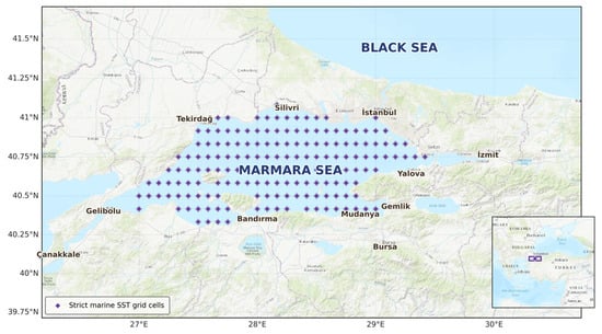
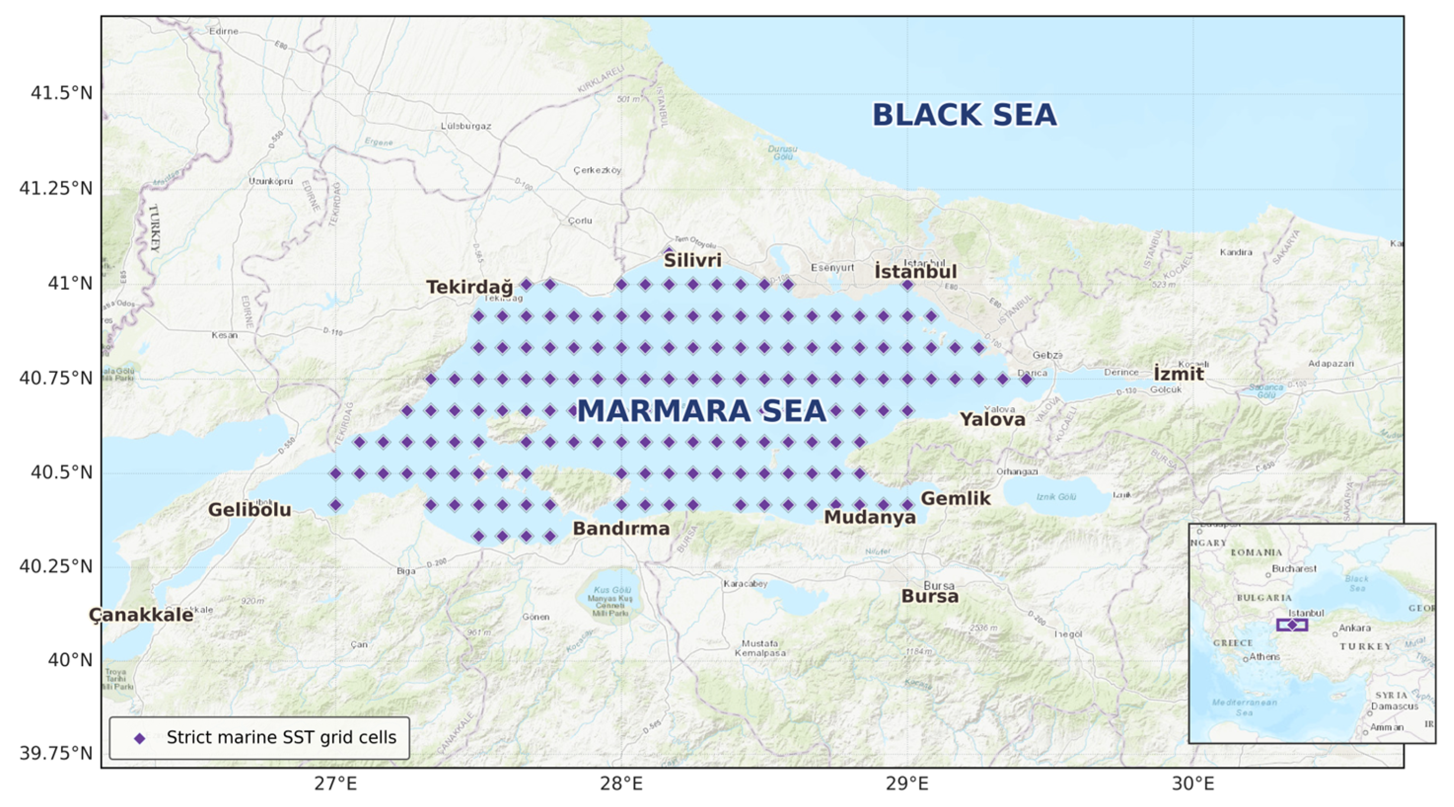
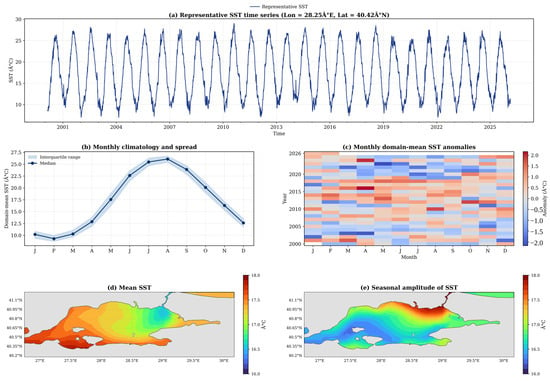
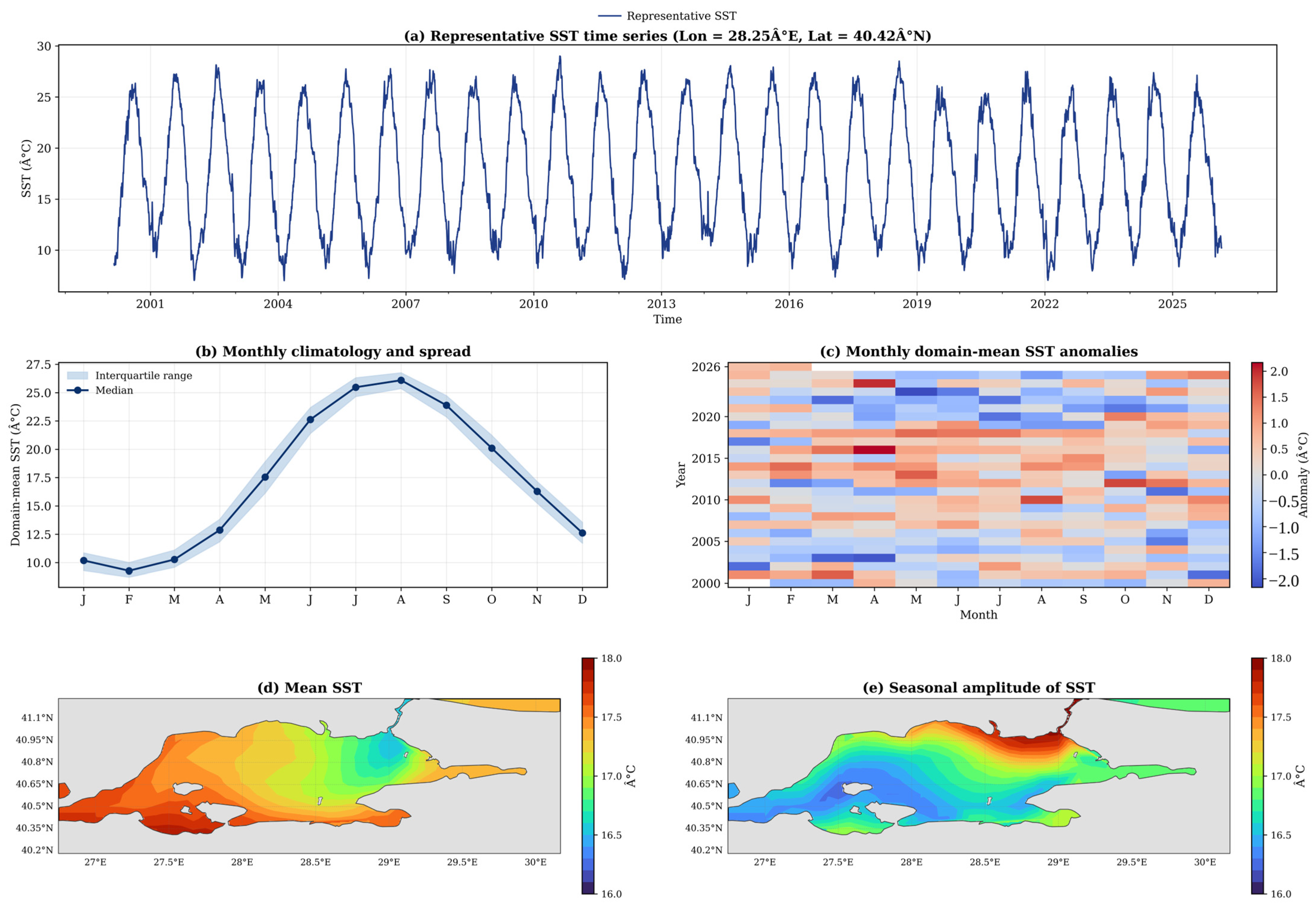
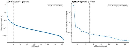
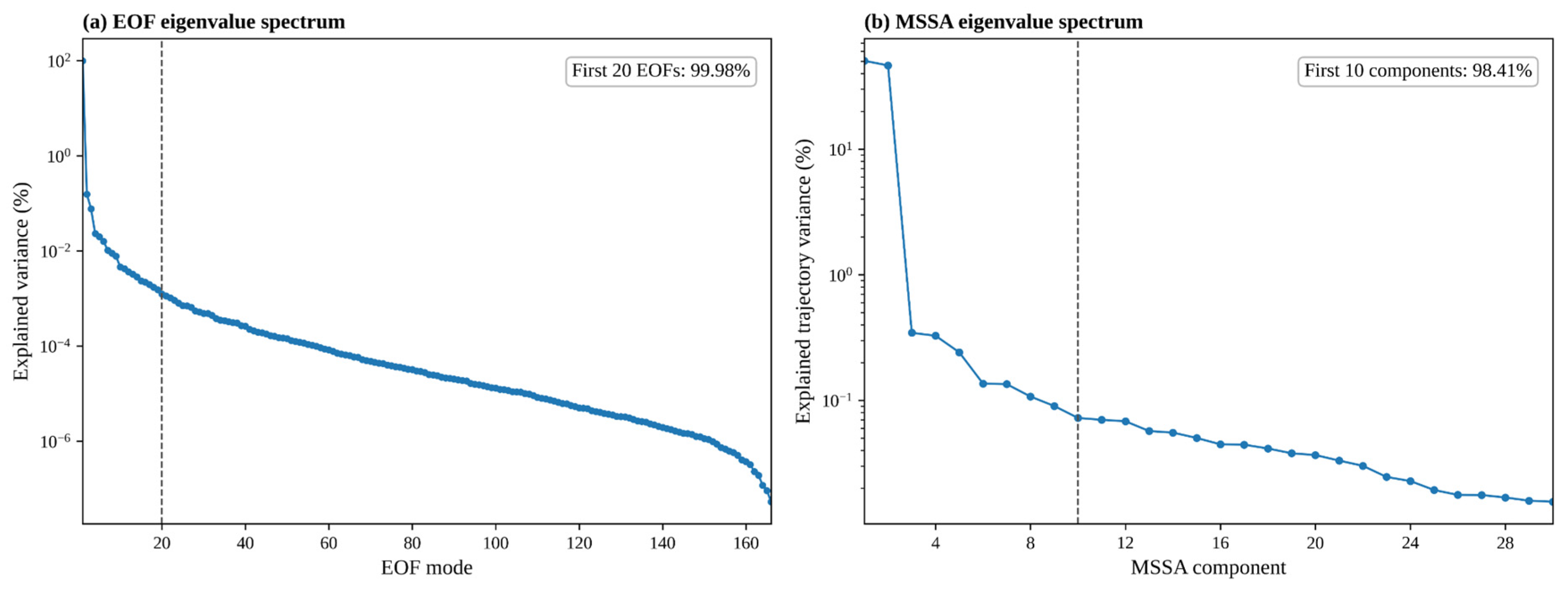
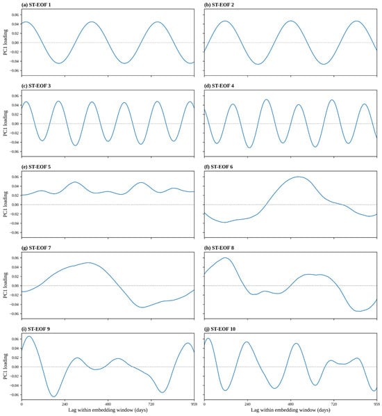
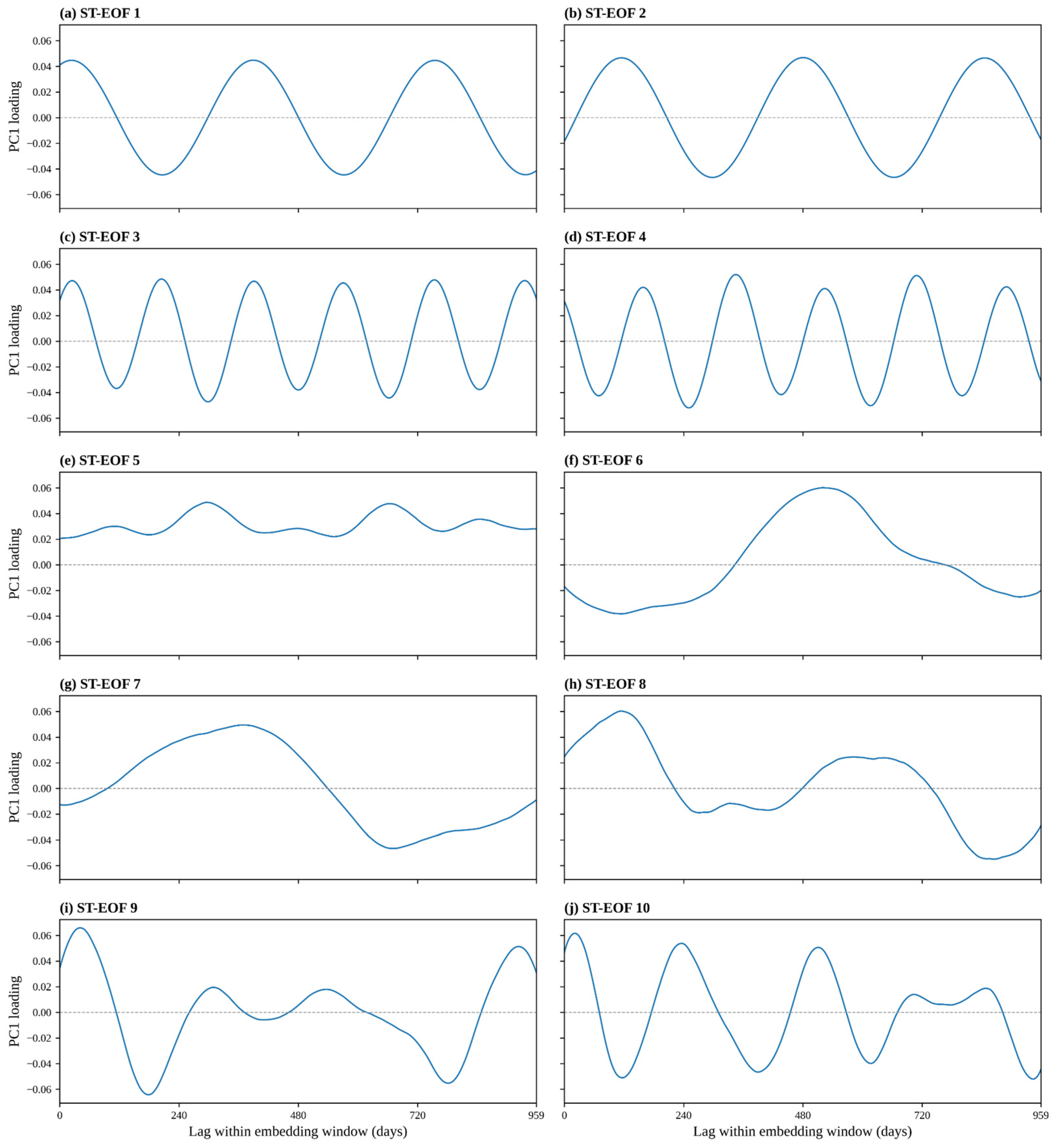
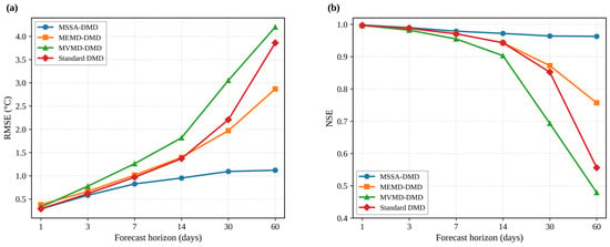
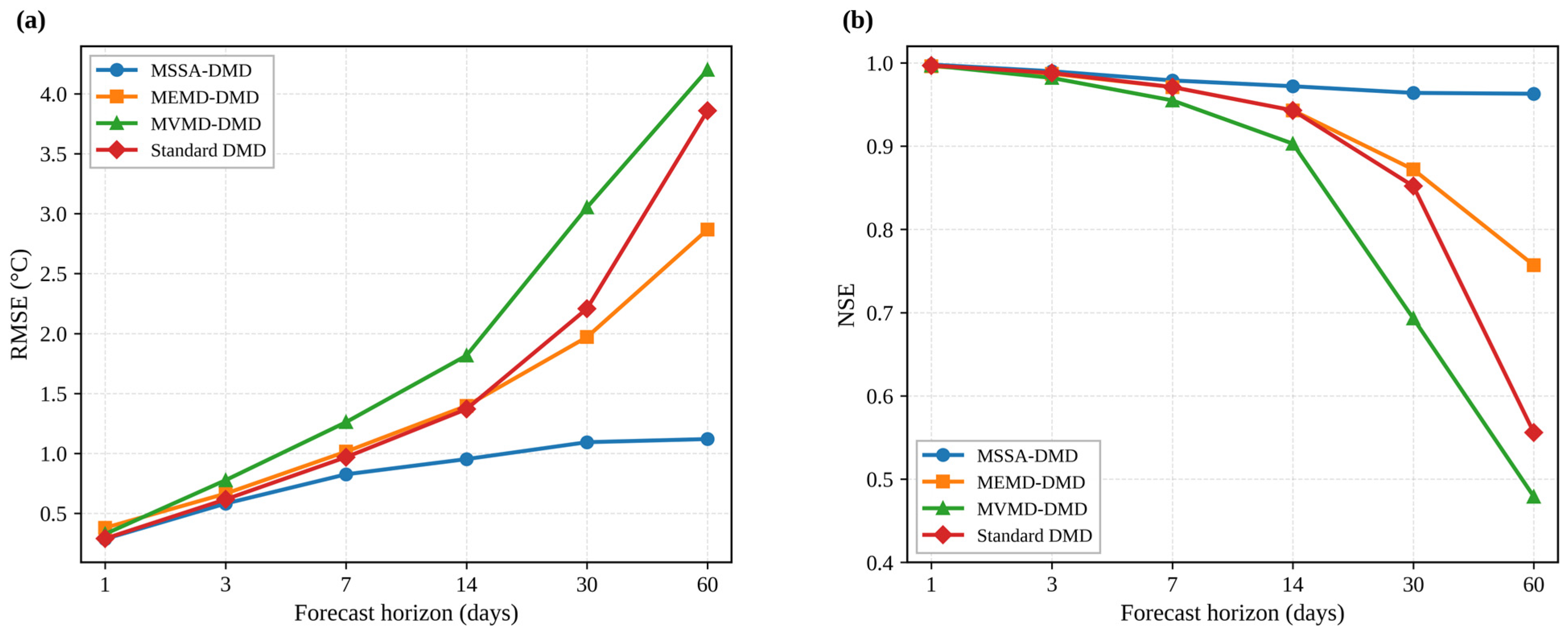
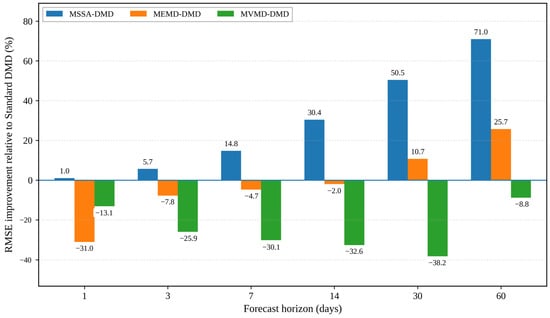
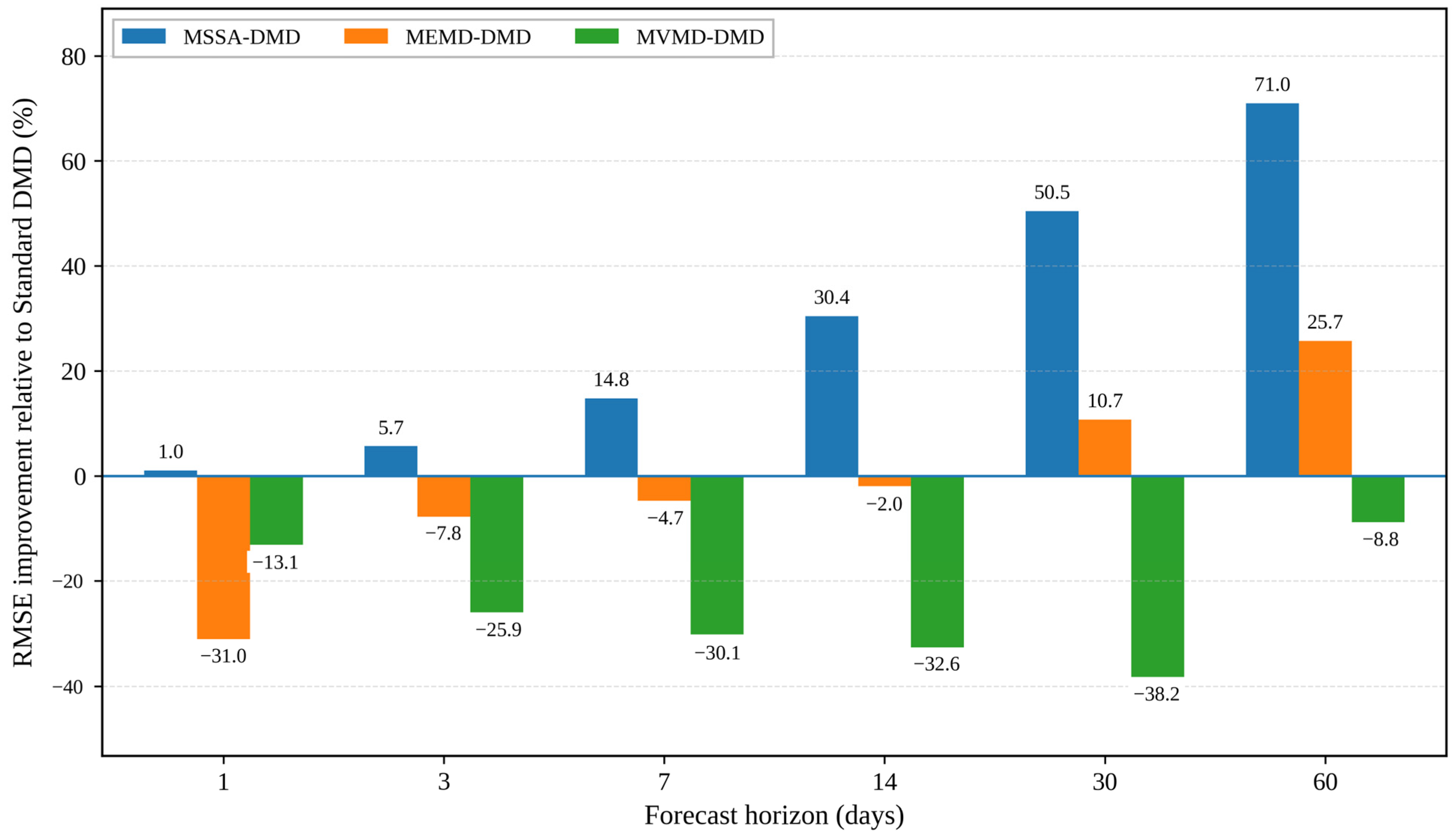
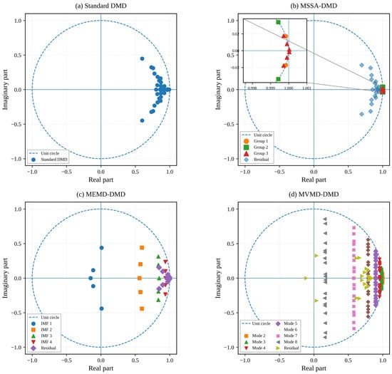
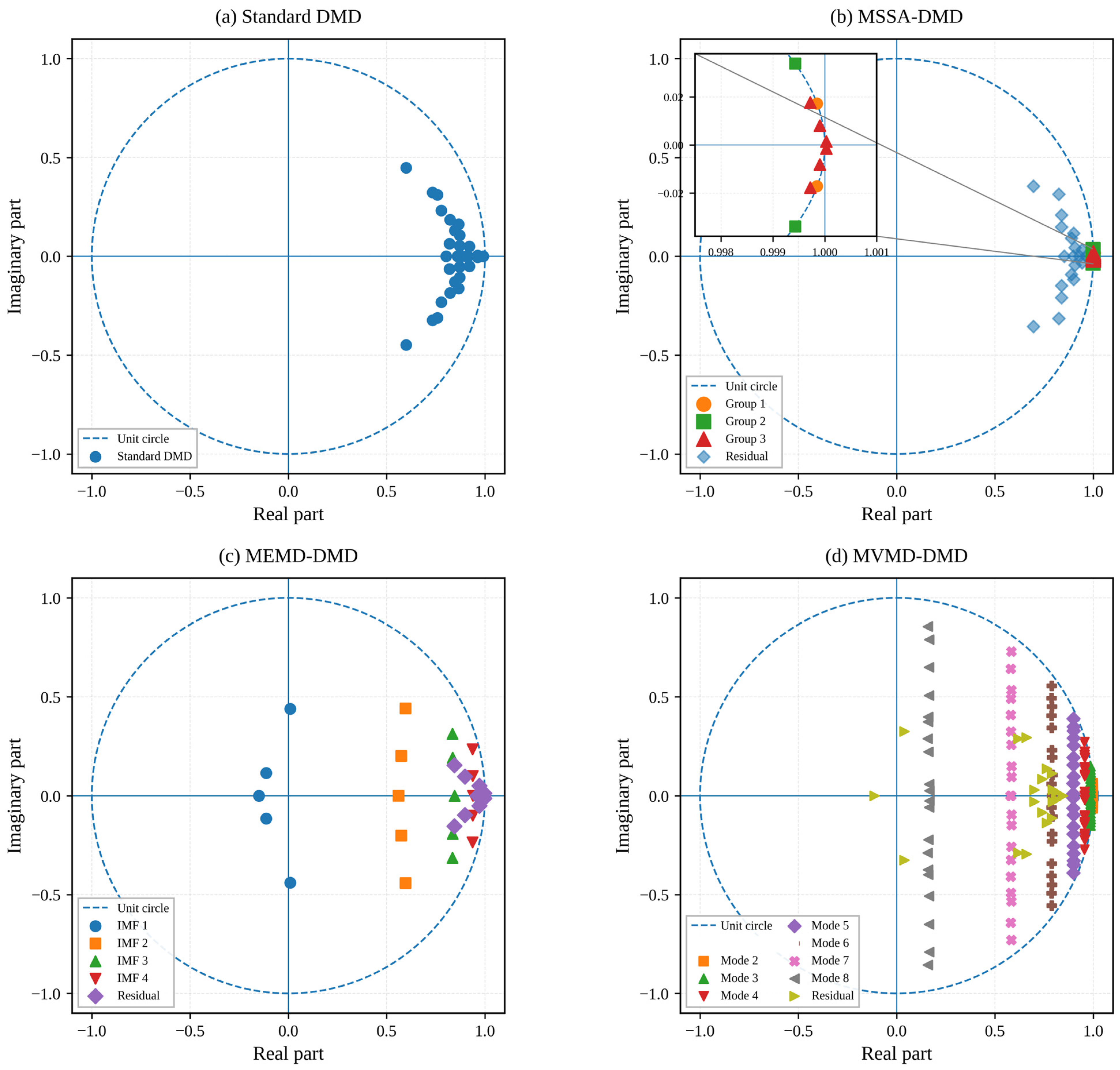
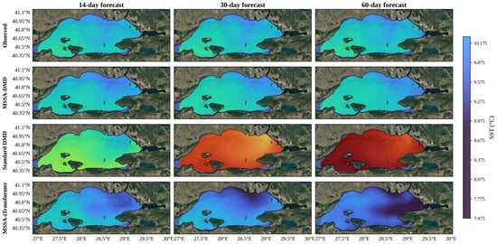
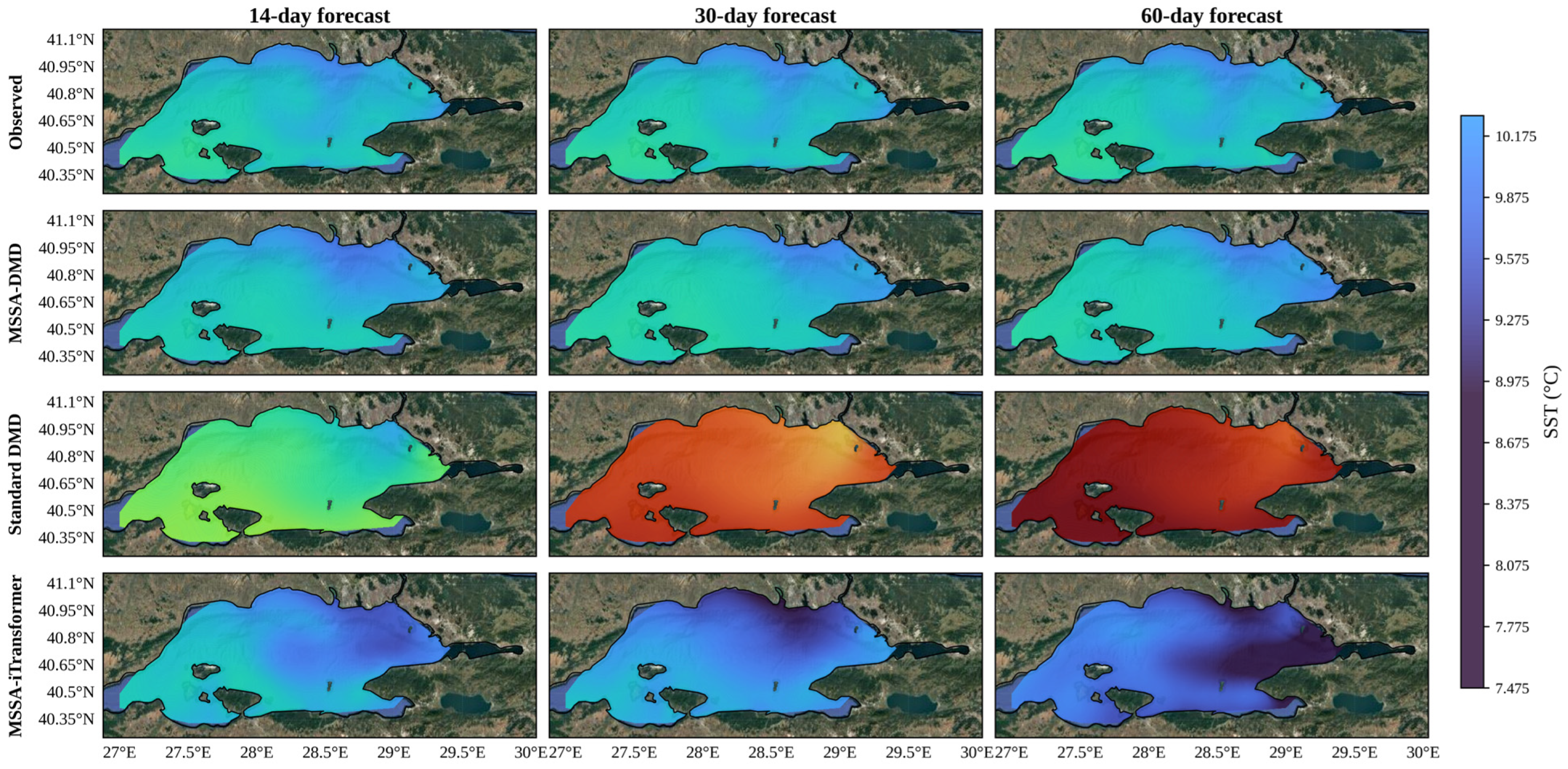
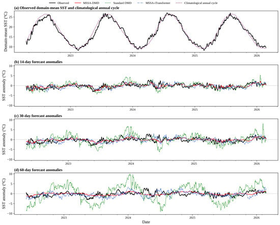
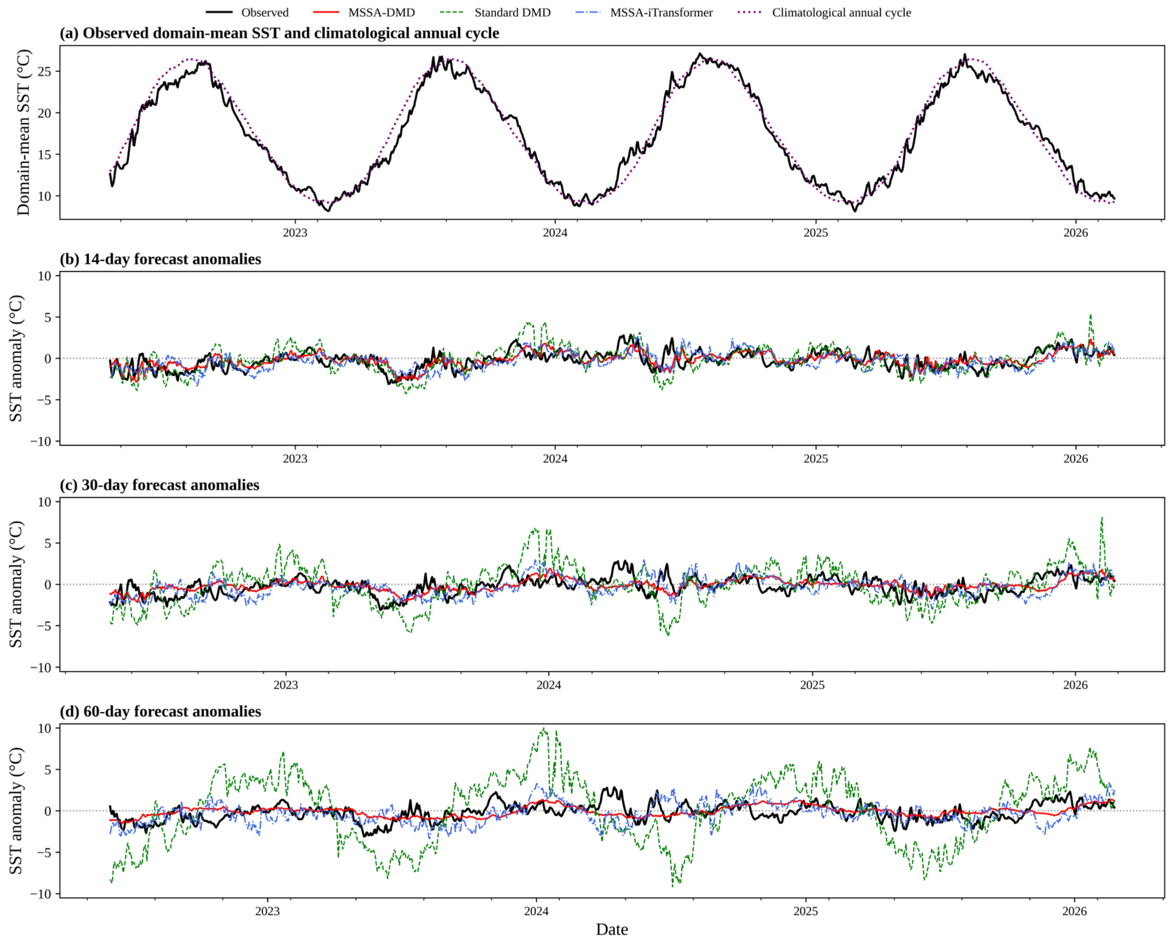
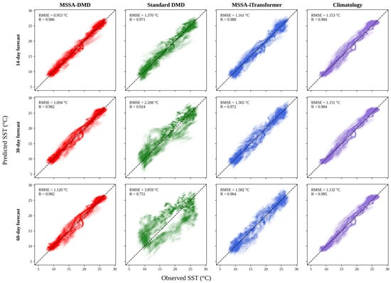
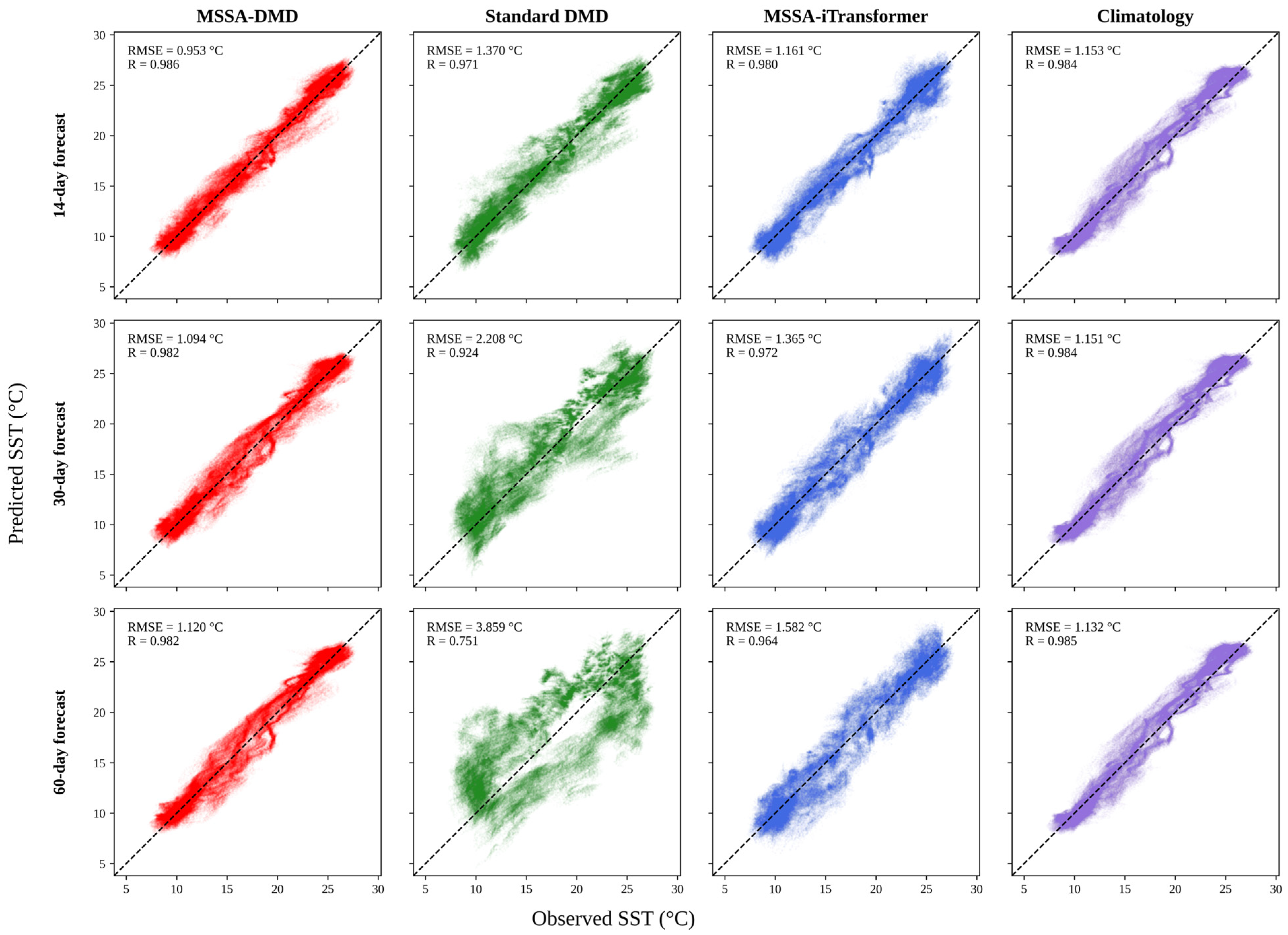
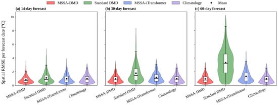
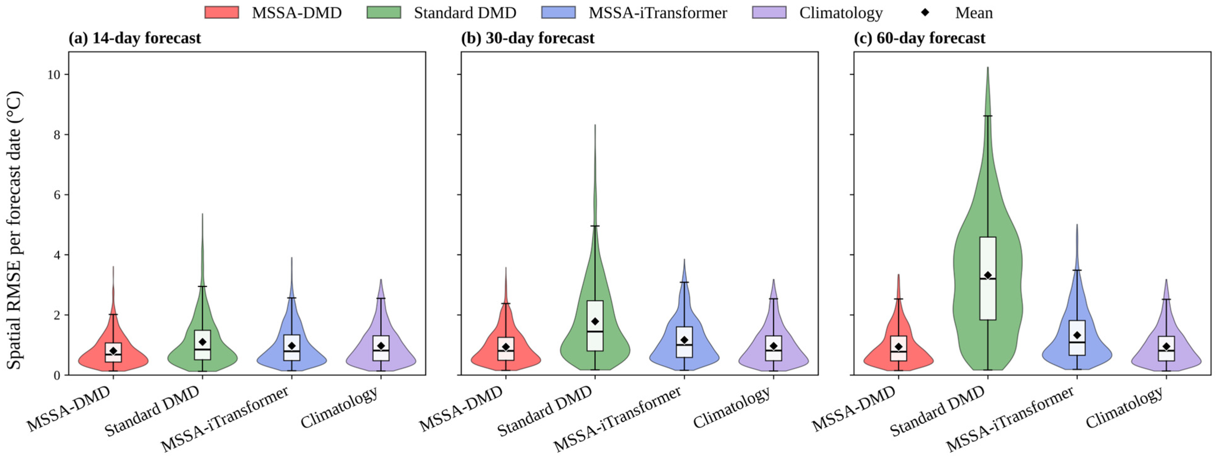
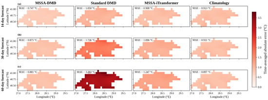
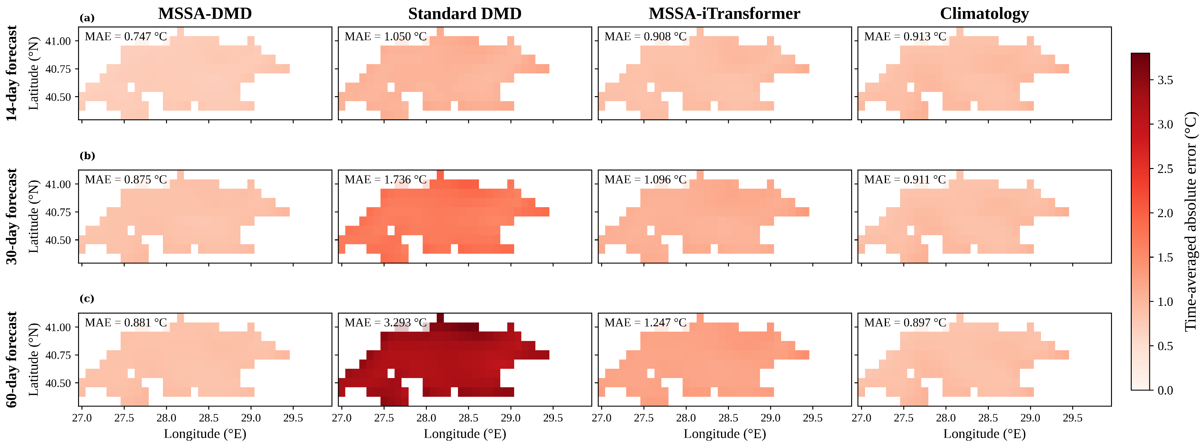

Disclaimer/Publisher’s Note: The statements, opinions and data contained in all publications are solely those of the individual author(s) and contributor(s) and not of MDPI and/or the editor(s). MDPI and/or the editor(s) disclaim responsibility for any injury to people or property resulting from any ideas, methods, instructions or products referred to in the content. |
© 2026 by the author. Licensee MDPI, Basel, Switzerland. This article is an open access article distributed under the terms and conditions of the Creative Commons Attribution (CC BY) license.