An Adaptive Setting Optimization Algorithm for Debris Flow Early Warning Threshold Integrating Chaotic Gray Wolf Optimization and Internal Model Repetitive Control

Abstract

The effectiveness of early warning thresholds for debris flows is concurrently constrained by geological spatial heterogeneity and the cumulative effects of rainfall duration, with the coupling mechanisms between the two being complex and difficult to adapt dynamically. To address this issue, an adaptive optimization algorithm for debris flow early warning thresholds is proposed, integrating Chaotic Grey Wolf Optimization (CGWO) with Internal Model Repetitive Control (IMRC). This algorithm establishes a dual-layer linkage architecture of “offline global optimization + online periodic compensation”: CGWO solves for the optimal baseline thresholds for different types of susceptibility zones offline based on historical disaster data, while IMRC performs periodic compensation on the baseline thresholds according to real-time rainfall duration, thereby synergistically generating dynamic critical rainfall thresholds that account for both spatial zonation differences and rainfall temporal evolution. The method is validated in a debris-flow-prone mountainous watershed in Southwest China. The results indicate that the IMRC compensation exhibits clear duration dependence and zonation differentiation. Under short-duration rainstorm conditions, IMRC provides positive compensation, with compensation amounts of +3.5 mm, +1.5 mm, and +12.0 mm for high, moderate, and low susceptibility zones, respectively. Under medium-duration rainfall conditions, the compensation amounts are −2.0 mm, −1.5 mm, and +7.0 mm, respectively. Under long-duration sustained rainfall conditions, the compensation amounts are differentially output according to zonal geological conditions, being +2.5 mm, −3.0 mm, and −1.0 mm, respectively. Based on the above dynamic thresholds, the three-tier yellow, orange, and red early warning intervals exhibit a comprehensive early warning efficiency index that steadily improves with the accumulation of historical samples, eventually converging to 0.98–0.99. These results fully demonstrate the adaptive optimization capability of the proposed algorithm in both spatial zonation and temporal evolution dimensions, providing a reliable quantitative basis for refined graded early warning of debris flows at the watershed scale.

1. Introduction

Mountainous watersheds have drastic topographic relief and frequent tectonic activity. These areas hold large volumes of loose deposits [1]. Under the monsoon climate, short-term heavy rainfall is concentrated in time. Combined with hydrological conditions, this leads to frequent rainfall-induced debris flows. Such disasters are highly sudden, extremely destructive, and pose prominent chain risks. They seriously threaten the lives and property of local residents and the safety of infrastructure along the route [2]. Critical rainfall is the core indicator for debris flow monitoring and early warning. Accurate and appropriate warning thresholds are key to supporting graded early warning and timely evacuation organization. For this reason, they have consistently been a research priority in geological disaster prevention and mitigation [3].

Scholars at home and abroad have conducted extensive exploration around the optimization of warning thresholds, mainly forming four research directions: dynamic process simulation, data-driven intelligent discrimination, mathematical and statistical threshold modeling, and adaptive dynamic threshold adjustment. In terms of dynamic process simulation, early research was mostly based on empirical formulas or simplified hydrological models, but in recent years, it has gradually developed into fully physical process modeling that couples rainfall, infiltration, runoff, and convergence debris flow initiation. Li et al. [4] used the SynxFlow coupling model to fully simulate the working conditions of debris flow crossing protective facilities under different rainfall intensities and durations. They optimized the threshold from the perspective of disaster losses and reduced the false alarm problem in engineering protection zones. However, this type of model usually fits a fixed I-D curve for a single watershed, without considering the differences in geological conditions within different zones of the watershed, and cannot dynamically adjust the critical rainfall based on the accumulated rainfall duration. The spatial differentiation and temporal adaptability are significantly insufficient. In terms of data-driven machine learning discrimination, as monitoring data accumulates, algorithms such as support vector machines, random forests, and deep neural networks are gradually introduced. Ikhsan et al. [5] extracted two core features, rainfall and duration, based on measured data from the Putih River Basin for predicting the probability of debris flows. However, this type of method currently mainly implements binary classification judgment of whether debris flows have occurred, and fails to quantify multi-level risk intervals such as yellow, orange, and red, making it difficult to support gradient disaster prevention scheduling. In terms of threshold modeling in mathematical statistics, fitting I-D and I-E empirical curves based on historical data is currently the most widely used method in watershed early warning operations. However, Zhang et al. [6] explicitly pointed out that traditional statistical methods generate errors and amplify them step by step from rainfall monitoring to threshold calculation, resulting in severe distortion of the final threshold. Although subsequent research has reduced some calculation errors by optimizing the layout of monitoring points and improving the structure of statistical models, it is essentially limited to improving the accuracy of static statistical thresholds and cannot achieve dynamic adaptive adjustment by region and working condition. In terms of adaptive threshold dynamic adjustment, some scholars have attempted to introduce dynamic correction mechanisms to enhance robustness. Xu et al. [7] confirmed that adaptive dynamic thresholds can synchronously reduce missed alarms and false alarms in line icing warning scenarios. However, this type of method is still in its infancy in the field of debris flow, and only makes local adjustments to a single judgment threshold, failing to achieve multi-level risk threshold quantification division under multi-regional and multi-condition coupling.

In summary, although existing research has been continuously deepened within various methodological frameworks, there are still common limitations: whether it is dynamic models, machine learning, or statistical methods, they are all based on the basic setting of “single watershed unified threshold” or “static fixed threshold”, have not effectively coupled the inherent differences in geological condition zoning in the spatial dimension, have not depicted the nonlinear disturbance law of rainfall duration accumulation on critical rainfall in the temporal dimension, and lack a systematic solution to incorporate the two into the threshold generation mechanism in synergy. In response to this research gap, the core contribution of this paper lies in: (1) introducing Chaos Grey Wolf Optimization (CGWO) and Internal Model Repetitive Control (IMRC) into the field of debris flow warning threshold setting, constructing a dual-layer linkage framework of “offline global optimization benchmark threshold + online periodic disturbance compensation”, and achieving collaborative decoupling and adaptive approximation of spatial differences and temporal effects from the algorithmic mechanism; (2) unlike previous studies that only optimize a single static threshold, this paper explicitly outputs the graded dynamic critical rainfall and multi-level warning intervals of yellow, orange, and red for high, medium, and low susceptibility areas under three types of rainfall duration conditions, forming an engineering deployable threshold query system, thereby expanding threshold optimization from “single point adaptive” to a complete adaptive framework of “zone condition multi-level”. Based on the long-term measured dataset of the watershed, the static benchmark thresholds of each area were solved offline through CGWO, and the IMRC module was introduced to calculate the real-time rainfall compensation for short, medium, and long rainfall conditions. Finally, dynamic adaptive critical rainfall was generated, and multi-level warning intervals were divided. The comprehensive early warning energy efficiency index (CWEEI) is used to quantitatively evaluate the optimization effect, verify the advantages of the proposed method in accuracy and stability, and provide a quantitative basis for judgment for fine debris flow classification early warning in the watershed.

2. Research on Adaptive Setting Optimization Algorithm for Debris Flow Warning Threshold

2.1. Regional Overview

The research area is located in the Heishui River Basin, a primary tributary of the Zemu River in the middle section of the Anning River Basin in Liangshan Prefecture, Sichuan Province (longitude 102°18′~102°32′ E, latitude 27°42′~27°56′ N). It is a high-risk area for debris flow disasters in mountainous areas, with a drainage area of about 320 km², a main ditch length of about 28 km, and a relative height difference of about 2600 m. The steep terrain, strong tectonic activity, and concentrated rainfall in the research area provide favorable terrain, material sources, and water sources for debris flow outbreaks.

In terms of geological conditions, the exposed strata in the study area are mainly Triassic sandstone and mudstone, interbedded with coal seams and thin layers of limestone. The strata have varied attitudes and well-developed joints and fractures. Affected by regional fault structures, the rock mass is strongly fractured, and the thickness of the surface weathered colluvial deposits is generally 3–15 m, with a loose structure, providing abundant solid material sources for debris flow initiation [8]. The study area has frequent historical earthquake activity, with an earthquake intensity of VIII. The earthquake action has aggravated slope instability and collapse accumulation, and a large amount of loose deposits are distributed on both sides of the main gully and tributary gullies, forming a debris flow material reserve. The main geological parameters of the study area are shown in Table 1.

Table 1. Main geological parameters of the study area.

Parameter Type	Parameter Name	Value/Characteristic
Topography and Geomorphology	Watershed Area	320 km2
Topography and Geomorphology	Main Gully Length	28 km
Topography and Geomorphology	Relative Elevation Difference	2600 m
Topography and Geomorphology	Average Longitudinal Slope Gradient	180‰
Stratum Lithology	Main Strata	Triassic sandstone, mudstone, coal seam, thin-bedded limestone
Stratum Lithology	Weathering Layer Thickness	3~15 m
Geological Structure	Fault Structure	Regional faults are well-developed, and rock mass joints are dense
Geological Structure	Seismic Intensity	VIII degree
Material Source Conditions	Collapse Accumulation Body	Widely distributed on both sides of the main and branch gullies
Material Source Conditions	Loose Accumulation Reserves	Approximately 12 million m3

In terms of climate and hydrological conditions, the study area belongs to the subtropical monsoon climate with distinct dry and wet seasons. The average annual precipitation is about 1100 mm, and the precipitation in the rainy season accounts for more than 85% of the annual precipitation, which is mostly manifested as short-duration heavy rainfall, with the maximum daily rainfall reaching 180 mm. The concentrated heavy rainfall and high soil moisture content in the early stage are the main triggering factors for debris flow outbreaks. The main hydrological parameters of the study area are shown in Table 2.

Table 2. Main hydrological parameters in the study area.

Parameter Type	Parameter Name	Value/Characteristic
Rainfall	Multi-year Average Precipitation	1100 mm
Rainfall	Proportion of Precipitation in Rainy Season	85%
Rainfall	Maximum Daily Precipitation	180 mm
Rainfall	Rainfall Type	Short-duration Heavy Rainfall, Local Torrential Rain
Soil Moisture	Saturated Moisture Content of Surface Soil	42%
Soil Moisture	Field Capacity	30%
Groundwater	Peak Pore Water Pressure	About 120 kPa
Runoff Generation and Concentration	Surface Runoff Coefficient	0.45~0.65

In Table 2, the soil moisture parameters are based on daily observation data from three automatic soil moisture monitoring stations (buried at depths of 10 cm, 20 cm, and 40 cm) in the study area from 2020 to 2025. The peak pore water pressure is taken from the measured records of vibrating-string pore water pressure gauges buried in the channel during typical debris flow events in the rainy season. The runoff coefficient is calculated based on the flow observation results of four hydrological sections set up in the study area, combined with the calibration of rainfall processes during the same period.

The complex geological structure background, material resources for debris flow, and extreme rainfall conditions mentioned above make debris flow disasters in this region have typical characteristics of high frequency, strong abruptness, and great destructive power, and it is a representative region for carrying out research on adaptive setting optimization of warning thresholds [9].

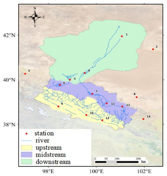
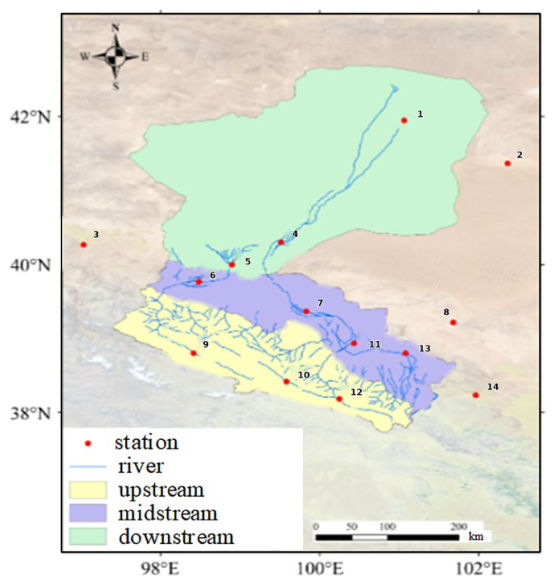
The data used in this study was sourced from 14 automatic meteorological and hydrological monitoring stations (covering the main area and six main tributaries with a data collection interval of 10 min) deployed in the research basin during the rainy season from 2018 to 2025 (May to October each year). The original rainfall records were formed into a complete event database after quality control. The location of the monitoring station is shown in Figure 1 (distribution map of monitoring stations in the study area).

Figure 1. Distribution map of monitoring stations in the research area.

The event screening criteria are: when the monitoring station records the initiation of a debris flow accompanied by a significant increase in rainfall, the continuous rainfall process is defined as an independent debris flow event, and incomplete events due to equipment failure or data loss are excluded. Table 3 fully includes the core hydrological observation data of 20 debris flow events in the basin during the rainy season, including three core indicators: disaster start and end time, rainfall duration, and cumulative rainfall. Among them, there are five large-scale debris flow events marked with *.

Table 3. Statistical data of debris flow events.

Debris Flow Event No	Start Time/Year-Month-Day Time	End Time/Year-Month-Day Time	Rainfall Duration/h	Rainfall/mm
1	2023/7/11 16:00	2023/7/11 21:00	5	27.5
2	2023/7/12 1:00	2023/7/12 6:00	5	13.2
3	2023/7/12 20:00	2023/7/13 3:00	7	37.6
4 *	2023/7/13 13:00	2023/7/13 20:00	7	22.5
5 *	2023/7/14 3:00	2023/7/14 8:00	5	18.3
6 *	2023/7/25 22:00	2023/7/26 7:00	9	37.9
7	2023/7/26 21:00	2023/7/27 2:00	5	7.8
8	2023/7/30 21:00	2023/7/31 0:00	3	29.5
9	2023/8/6 15:00	2023/8/6 17:00	2	15.2
10	2023/8/6 21:00	2023/8/7 4:00	7	14.8
11	2023/8/10 0:00	2023/8/10 10:00	10	37.5
12 *	2023/8/11 18:00	2023/8/12 8:00	14	99.2
13	2023/8/17 22:00	2023/8/18 6:00	8	52.5
14	2023/8/18 20:00	2023/8/19 6:00	10	23.6
15 *	2023/8/19 20:00	2023/8/20 10:00	14	101.5
16	2023/8/20 20:00	2023/8/21 8:00	12	10.2
17	2023/8/23 16:00	2023/8/23 17:00	1	8.1
18	2023/8/23 20:00	2023/8/24 1:00	5	33.5
19	2023/8/24 4:00	2023/8/25 7:00	27	42.3
20	2023/8/26 18:00	2023/8/27 0:00	6	15.1

Note: Serial numbers marked with * indicate larger debris flow events.

The 20 historical events in Table 3 are mainly used to reveal the disaster-causing laws and multi-factor coupling characteristics of debris flows in the watershed, providing a physical basis for the construction of an early warning indicator system. The 27 sets of samples (9 from high, medium, and low susceptibility areas each) used for the calibration of the CGWO-IMRC algorithm are derived from new observation data (rainy season 2024–2025) that are independent and non-overlapping with the samples listed in Table 3. These two sets of data together form the dual basis for modeling and validation. Although 27 sets of calibration samples have covered the complete gradient range of rainfall conditions for debris flow initiation in three geological zones (cumulative rainfall of 36–100 mm, rainfall duration of 7–31 h), the sample size is still limited compared to the algorithm’s claimed adaptive ability and convergence accuracy of 0.98–0.99, which may pose certain constraints on the model’s generalization ability. To objectively evaluate the performance of the algorithm and enhance the statistical robustness of the conclusions, this study introduced a K-fold cross-validation strategy (K = 5) in the model training and validation stages. The 27 sets of samples were randomly divided into five subsets, with one subset rotated as the validation set and the remaining four subsets as the training set. The performance indicators were averaged five times to reduce evaluation bias caused by single partitioning. At the same time, in the results analysis section, the overfitting risk that may arise from limited sample size is clearly explained, and the threshold output of the algorithm in practical applications is limited to the rainfall parameter range covered by this study (cumulative rainfall of 8–101.5 mm, rainfall duration of 1–27 h). When exceeding this range, it is necessary to gradually extrapolate based on on-site monitoring data to avoid blind extrapolation leading to warning failure. The above measures aim to maximize the reliability of model evaluation and the credibility of conclusions under existing data conditions, laying the foundation for algorithm iteration optimization under richer sample conditions in the future.

As shown in Table 3, the duration of rainfall is the core temporal factor controlling the scale of debris flows: a short duration (1–3 h) of weak rainfall can trigger small-scale debris flows, indicating a high sensitivity of the watershed to sediment sources; long-duration (≥9 h) continuous rainfall is the core prerequisite for large-scale debris flows, with 3 out of 5 large-scale debris flows being long-term rainfall. Long-duration rainfall is an important triggering condition for large-scale debris flows.

Accumulated rainfall determines the level of debris flow disasters: rainfall shows a clear three-level disaster gradient, with <20 mm triggering only small low-risk debris flows, 20–40 mm being the high-frequency disaster core area of the watershed (including three large-scale debris flows), and >40 mm being the exclusive area for extreme disasters (including two super large debris flows). Table 3 also reveals the significant characteristics of concentrated and continuous outbreaks of debris flows: multiple debris flows occurred consecutively within a few days from 11–14 July, 6–7 August, 17–20 August, and 23–25 August in 2023. After multiple previous rainfall events, large-scale mud and stone flows also occurred with smaller rainfall amounts, indicating that the superposition of rainfall time series will change the conditions for debris flow initiation, and fixed warning thresholds cannot adapt to continuous rainfall scenarios.

The disaster caused by debris flows is the result of the coupling of multiple factors: both high rainfall intensity and short duration, and low rainfall intensity and long duration can trigger debris flows. Large-scale debris flows are divided into two categories: the extreme mode of “long duration + high rainfall” and the superimposed mode of “medium short duration + early accumulated rainfall”. It is necessary to construct a multi-factor coupled early warning system.

Based on the comprehensive data of 20 events in the table, the core adaptability issue of traditional fixed warning thresholds can be clearly observed: the scale and level of debris flows are simultaneously affected by three core factors: rainfall duration, cumulative rainfall, and temporal continuous outbreak characteristics. Relying solely on a single indicator cannot achieve accurate warning, and a multi-indicator coupled warning threshold system must be constructed to adapt to the complex disaster-causing laws of debris flows in the watershed.

Considering the differences in geological conditions in the study area, based on three different geological susceptibility zones (high susceptibility zone, medium susceptibility zone, and low susceptibility zone), nine typical debris flow events were selected from independent observation data during the rainy season from 2024 to 2025, forming new observation samples that are independent and non-overlapping with the samples in Table 3 (also sourced from the 12 monitoring stations mentioned above, using the same 10 min sampling interval and quality control process). The sample division is based on the differences in geological conditions in Table 4: the high-prone area has fractured structures, low permeability, and abundant sediment sources; the medium-prone area has moderate geological conditions; and the low-prone area has intact rock masses, good drainage, and scarce sediment sources, as detailed in Table 4.

Table 4. Statistical table of research area division and geological conditions.

Regional Division Type	Overall Distribution Characteristics of the Region	Detailed Geological Conditions
Areas with high susceptibility to mudslides	The valley is deeply incised, and the mountainous area is vast, making it a concentrated area for debris flows in the study area. Large debris flows mostly occur in this area	Overview of detailed geological conditions: Fault structures are widely distributed in the area, with developed rock fractures and a high degree of fragmentation, and the overall stability of the rock and soil is low. The surface is covered with a thick layer of weathered residual slope deposits, with abundant reserves of loose accumulations of gravel and sediment. The slope of the mountain is steep, and the ditch has a large drop. After rainfall infiltration, the soil is prone to slip and failure. The permeability of the soil is relatively weak, and rainwater is easily collected internally. The pore water pressure of the soil increases rapidly, and under the same rainfall conditions, it is more likely to form debris flows
Areas prone to mudslides	Flat plateaus and mountains are interspersed, and conventional small-scale debris flows are distributed in this area	Only small secondary faults exist locally, with moderate rock integrity, and some slopes have weak interlayers. Loose deposits are only concentrated on both sides of the valley and at the foot of the slope, and the thickness of the weathered soil layer on the slope surface is generally moderate. The slope of the mountain is moderate, the connectivity of the valleys is average, and the flow distance after soil instability is limited. The soil has moderate permeability and requires longer or greater accumulated rainfall to cause slope instability
Low-risk area for debris flow	The overall terrain is flat, mainly consisting of wide valleys, with only sporadic occurrences of very small slope mudflows and no records of large mudflows	The geological structure is simple and single; the rock mass is complete and hard, and there is no large-scale fractured zone. The bedrock has strong weathering resistance, and the loose soil layer on the surface is thin, resulting in a scarcity of solid material sources that can participate in debris flow movement. The slope is gentle, and the channel is wide and flat, lacking the dynamic conditions required for debris flow. The soil drainage effect is good, and rainwater is difficult to retain for a long time, which raises the pore water pressure and is less likely to induce mudslides

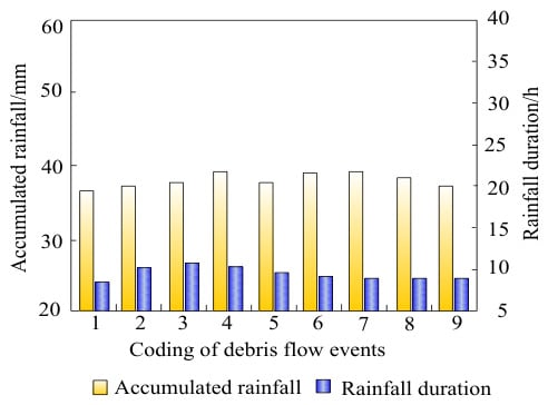
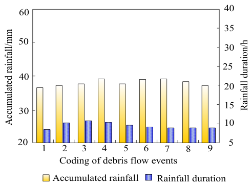
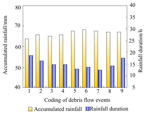
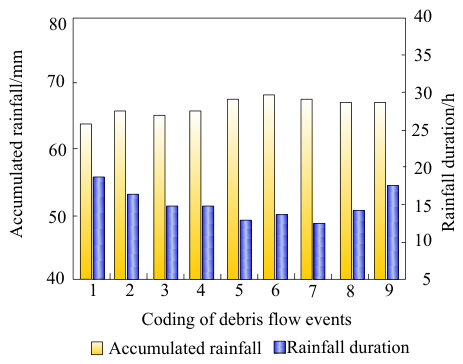
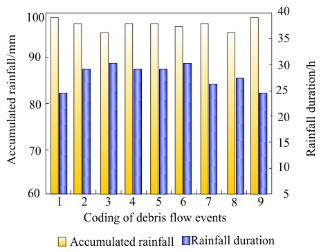
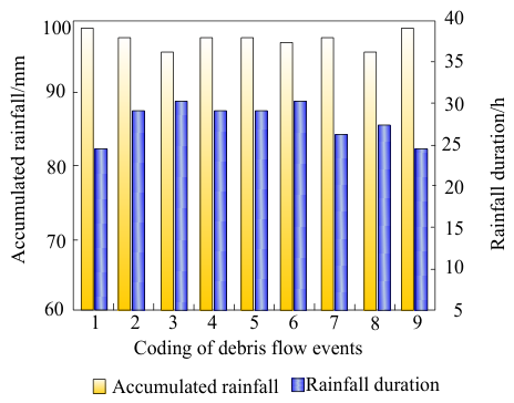
Combining synchronous rainfall monitoring data from the three areas, under the same rainfall input, the debris flow triggering behavior in the three areas shows significant differentiation, as detailed in Figure 2, Figure 3 and Figure 4.

Figure 2. Synchronous rainfall monitoring data in high-risk areas.

Figure 3. Synchronized rainfall monitoring data in the central prone area.

Figure 4. Synchronized rainfall monitoring data in low-risk areas.

In the graph, the yellow bars represent the cumulative rainfall (mm) required to trigger a debris flow, and the blue bars represent the corresponding rainfall duration (h). All three sets of graphs statistically analyze nine typical debris flow event monitoring samples, visually demonstrating the gradient differences in rainfall conditions required to trigger debris flows under different geological conditions. Detailed characteristics are as follows:

(1)

Features of rainfall data in high-risk areas in Figure 2

Cumulative Rainfall: The rainfall required to trigger the nine debris flow events is concentrated in the 36–40 mm range, representing the lowest rainfall level among the three types of areas. The peak event 4 had a peak rainfall of approximately 39 mm, while the remaining events mostly fluctuated between 36 and 38 mm, indicating that even small amounts of rainfall can trigger a disaster.

Rainfall Duration: The duration of rainfall is concentrated between 7 and 11 h, with the shortest overall duration being only 7 h. Most events lasted no more than 10 h.

(2)

Features of rainfall data in medium-risk areas in Figure 3

Cumulative rainfall: The rainfall range for debris flow initiation is 63~68 mm. The overall rainfall level is significantly higher than that of high-risk areas. The peak events 6 and 7 are about 68 mm, and the rainfall base is significantly higher.

Rainfall Duration: The duration of rainfall is distributed between 10 and 18 h, with a slight overlap with high-risk areas, but the overall average is longer, reaching a maximum of 16 h.

(3)

Features of rainfall data in low-risk areas

Cumulative Rainfall: The rainfall at the start of all events was in the range of 96–100 mm, the highest among the three types of areas, with most samples approaching 100 mm. Debris flows were only triggered under extreme heavy rainfall conditions.

Rainfall Duration: The duration of rainfall was stably distributed between 24 and 31 h, with continuous rainfall duration far exceeding that of high- and medium-risk areas, indicating prolonged and continuous overcast and rainy weather.

In summary, a single, fixed debris flow warning threshold cannot adapt to the differentiated disaster-causing patterns of different geological zones in the watershed, nor can it cope with the dynamic changes in activation conditions brought about by continuous rainfall [10]. Therefore, it is urgent to construct an adaptive warning threshold optimization method that can distinguish between high-, medium-, and low-risk areas and can be adjusted in real time according to the rainfall sequence. This paper proposes an optimization algorithm that integrates chaotic gray wolf optimization and Internal Model Repetitive Control to realize the adaptive setting of debris flow warning thresholds in multiple regions and dynamics.

2.2. Research Methods

This paper proposes an adaptive threshold setting algorithm that integrates chaotic gray wolf optimization and Internal Model Repetitive Control. The algorithm consists of two stages: offline benchmark optimization and online dynamic compensation. CGWO solves the optimal static benchmark threshold for each partition offline based on historical disaster samples, while IMRC performs periodic compensation on the benchmark threshold based on real-time rainfall duration, ultimately outputting a dynamic warning threshold that takes into account both spatial partition differences and the cumulative effect of time.

2.2.1. Chaotic Gray Wolf Optimization—Offline Benchmark Threshold Optimization

CGWO searches for the optimal threshold benchmark Λ_b on the historical dataset S to minimize the early warning error rate [11]. Suppose the debris flow monitoring system collects m types of monitoring data at discrete time t.

$$s(t)={[s_1(t),s_2(t),\dots ,s_m(t)]}^{\mathrm{T}}$$

(1)

The early warning threshold baseline vector is defined as:

$${\mathsf{\Lambda }}_{\mathrm{b}}={[{\lambda }_{\mathrm{b},1},{\lambda }_{\mathrm{b},2},\dots ,{\lambda }_{\mathrm{b},m}]}^{\mathrm{T}}$$

(2)

where λ_b,i is the reference threshold of the ith type of monitoring factor, determined by CGWO offline optimization.

The real-time early warning threshold vector is:

$$\mathsf{\Lambda }(t)={[{\lambda }_1(t),{\lambda }_2(t),\dots ,{\lambda }_m(t)]}^{\mathrm{T}}$$

(3)

The debris flow comprehensive early warning index is defined as the square root of the weighted sum of squares of the normalized deviation of each factor:

$$\Gamma \left(t\right)=\sqrt{{\displaystyle \sum _{i=1}^6{\rho }_i{\left(\frac{{\lambda }_i\left(t\right)-{\eta }_i}{{\lambda }_i\left(t\right)}\right)}^2}}$$

(4)

where ρ_i is the expert weight of the ith channel; η_i is the historical average of the monitoring values of the ith channel during the disaster-free period; λ_i(t) is the dynamic threshold of the ith channel at time t. An early warning is triggered when Γ(t) ≤ Γ_th, Γ_th is a fixed global early warning scalar threshold.

The fitness function of CGWO is the mudslide warning error rate of the historical dataset S:

$$\Phi \left(\mathsf{\Lambda }\right)={\displaystyle \frac{1}{\left|S\right|}}{\displaystyle \sum _{t\in S}\left[{ℂ}_{\left\{\Gamma \left(t\right)\ge {\Gamma }_{\mathrm{th}},z\left(t\right)=0\right\}}+{ℂ}_{\left\{\Gamma \left(t\right)<{\Gamma }_{\mathrm{th}},z\left(t\right)=1\right\}}\right]}$$

(5)

where |S| is the total number of samples in the dataset S; z(t) ∈ {0,1} is the true state label (0 indicates no mudslide, 1 indicates mudslide); ℂ is the indicator function (1 if the condition is met, 0 otherwise). The first item counts the number of false alarms, the second item counts the number of missed alarms, and the sum of the two items accounts for the proportion of the total samples, which is the warning error rate [12].

The individual position vector of CGWO is the warning threshold reference vector Λ_b. The core parameters of the algorithm are set as follows: the population size is set to 30, the maximum number of iterations is 500, the chaotic disturbance trigger interval is 5 iterations, and the termination condition is that the optimal fitness value changes by less than 10⁻⁴ or reaches the maximum number of iterations in 20 consecutive iterations. The population is initialized using the Tent chaotic mapping:

$${\chi }_{n+1}=\left\{\begin{array}{cc}{\chi }_n/0.7,& 0<{\chi }_n\le 0.7\\ \left(1-{\chi }_n\right)/0.3,& 0.7<{\chi }_n<1\end{array}\right.$$

(6)

where χ_n is the n th chaotic sequence value. The specific initialization process is as follows: first, randomly generate an initial value between (0, 1), then iteratively generate N chaotic sequences using Equation (6), discard the first 500 transient points to eliminate initial value sensitivity, and take the subsequent N sequence values to form the initial chaotic sequence set.

The position of the ith initial individual is mapped to the solution space:

Λ_b,i(0) = Λ_min + χ_i ⋅ (Λ_max − Λ_min),i = 1,2,…,N

(7)

where N is the population size; Λ_min, Λ_max are the upper and lower bounds of the search for the warning threshold benchmark; χ_i is the ith value of the Tent sequence. Calculate the fitness (warning error rate) of each candidate threshold benchmark [13], and take the top three in ascending order Λ_α, Λ_β, Λ_δ. The three-headed leader wolf guides the candidate threshold baseline position Λ₁, Λ₂, Λ₃, and the final threshold baseline position of the individual takes the average Λ_b(t + 1) of the three; every 5 iterations, a chaotic perturbation is applied to Λ_α to prevent the current best individual from falling into a local optimum [14]. The position update adopts the linear decreasing convergence factor strategy of the standard grey wolf algorithm, which linearly decreases from 2 to 0. The perturbation formula is:

$${{\mathsf{\Lambda }}^{\prime }}_{\mathsf{\alpha }}\left(t\right)={\mathsf{\Lambda }}_{\mathsf{\alpha }}\left(t\right)+\omega \left(t\right)\cdot \left(2\chi -1\right)\cdot {\mathsf{\Lambda }}_{\mathsf{\alpha }}\left(t\right)$$

(8)

where ω(t) is the perturbation amplitude that decays with iteration, χ is the current Tent chaotic value. If the fitness after perturbation is ${\Phi }_{\mathrm{c}}\left({{\mathsf{\Lambda }}^{\prime }}_{\mathsf{\alpha }}\right)<{\Phi }_{\mathrm{c}}\left({\mathsf{\Lambda }}_{\mathsf{\alpha }}\right)$, then replace Λ_α with the perturbed individual ${{\mathsf{\Lambda }}^{\prime }}_{\mathsf{\alpha }}$.

Stop when the change in the optimal early warning error rate is less than ε_c = 10⁻⁵, and output the optimal early warning threshold benchmark.

$${\mathsf{\Lambda }}_{\mathrm{b}}^{*}={\left[{\mathsf{\Lambda }}_{\mathrm{b},1}^{*},\dots ,{\mathsf{\Lambda }}_{\mathrm{b},m}^{*}\right]}^{\mathrm{T}}$$

(9)

In the fitness evaluation process, to reduce the sensitivity of small sample partitioning and enhance the robustness of the model’s generalization ability, a five-fold cross-validation (K = 5) strategy is introduced. This strategy is only used for fitness calculation in the offline optimization stage of CGWO and does not participate in independent testing of the final warning performance. The specific implementation steps are as follows: stratified random sampling will be conducted on 27 sets of calibration samples according to the type of susceptibility zone (high/medium/low), ensuring that the proportion of samples in each of the three zones is consistent with the entire set (each fold contains about three groups of high, medium, and low susceptibility zones). Stratified sampling aims to preserve the impact of geological zone heterogeneity on threshold optimization; randomly divide the stratified samples into five subsets, and rotate one subset as the validation set and the remaining four subsets as the training set; at each compromise, CGWO only calculates fitness (warning error rate) on the current training set and records the validation error rate on the current validation set; the final fitness of the current individual is taken as the arithmetic mean of the 50% validation error rate, which serves as the optimization objective for the candidate threshold benchmark to participate in the iterative update of CGWO. Cross-validation only guides the threshold search direction during the CGWO iteration process and does not replace the performance evaluation of the final model on an independent test set. The optimal benchmark threshold for the final output is the global optimal solution learned from all 27 sets of samples based on the criterion of minimizing the 5-fold average validation error rate.

After the 5-fold cross-validation-guided search, the final optimal baseline threshold vector is retrained on the entire set of 27 calibration samples using the same CGWO procedure, with the convergence criterion unchanged. This ensures that the final output threshold fully utilizes all available calibration data while benefiting from the cross-validation-based search direction.

2.2.2. Internal Model Repeated Control (IMRC)—Real-Time Warning Threshold Periodic Compensation

After CGWO outputting the optimal warning threshold reference ${\mathsf{\Lambda }}_{\mathrm{b}}^{*}$, it is essentially a static fixed value and cannot respond to the changes in soil saturation caused by the accumulation of rainfall duration and the drift of the initiation conditions [15]. The actual debris flow triggering process is significantly affected by the evolution of rainfall time sequence. The deterioration mechanism of slope stability by short-term heavy rainfall and long-term continuous rain is completely different. The fixed benchmark threshold is difficult to take into account for such dynamic disturbances. Therefore, based on the CGWO offline benchmark, the IMRC module is further introduced to utilize its memory and compensation characteristics for periodic disturbances [16]. The threshold compensation amount is dynamically calculated according to the real-time rainfall duration, so that the warning critical value can be adaptively adjusted with the rainfall process [17].

The core value of the IMRC module is not to deal with the static statistic of “rainfall duration”, but to address the progressive and quasi-periodic evolution dynamics of soil saturation and pore water pressure during the accumulation process of rainfall duration. As an input indicator of CGWO, rainfall duration can only characterize the fact of “how much rainfall has been experienced”, but cannot describe the differential degradation effect of the same cumulative rainfall on slope stability at different times—for example, a rainfall that lasts for 10 h has a completely different destructive effect on soil at the 3rd and 8th hours. This threshold dynamic relaxation phenomenon driven by the rainfall process is essentially a time-varying disturbance with quasi-periodic characteristics, which cannot be captured by offline-optimized static benchmark thresholds. Therefore, CGWO determines the benchmark warning threshold values for each zone in the initial saturation state offline based on historical samples, and solidifies the differences in geological zones into prior biases; IMRC, on the other hand, uses this benchmark value as the initial reference during each rainfall process. Based on the spectral analysis results of real-time rainfall duration, it applies periodic phase advance compensation to the benchmark threshold, dynamically adjusting the warning critical value with the actual accumulation rate of soil saturation during the rainfall process. The compensation amount depends on the phase deviation of the current rainfall process relative to the historical period disturbance, rather than the absolute value of the rainfall duration. This precisely responds to the temporal superposition effect that cannot be handled by the fixed threshold of “small rainfall triggering large debris flows after multiple previous rainfall events”. In summary, IMRC transforms rainfall duration from a static indicator to a dynamic driving factor, endowing the threshold with the temporal ability to adaptively respond to rainfall processes. This cannot be replaced by simply using rainfall duration as an input indicator for CGWO.

IMRC takes ${\mathsf{\Lambda }}_{\mathrm{b}}^{*}$ as the benchmark, performs real-time compensation on the warning threshold for quasi-periodic environmental disturbances [18], and outputs the final dynamic warning threshold Λ(t).

Deviation signal e(t) is defined as the difference between the optimal reference threshold and the actual warning threshold after IMRC compensation [19], and the internal model transfer function is:

$$H_{\mathrm{IM}}\left(\iota \right)={\displaystyle \frac{\nu \left(\iota \right){\iota }^{-\widehat{\tau }\left(t\right)}}{1-\nu \left(\iota \right){\iota }^{-\widehat{\tau }\left(t\right)}}}$$

(10)

where ι is a discrete shift operator, ν(ι) is a zero-phase-shift low-pass filter, $\widehat{\tau }\left(t\right)$ is the number of period sampling points estimated in real time at time t (dynamically adjusted according to the rainfall duration, for example, short-duration rainstorms correspond to short periods, and long-duration continuous rainfall corresponds to long periods [20]). The specific estimation process of $\widehat{\tau }\left(t\right)$ is as follows: firstly, sliding window sampling is performed on the continuous monitoring data of the current rainfall event, with a fixed window length of 1 h and a sampling frequency of 1 time/minute, in order to obtain the original time series; secondly, the sequence is subjected to spectral analysis using Fast Fourier Transform (FFT) to extract the periodic components corresponding to the peak power spectral density; finally, the periodic component is converted into discrete sampling points and smoothed using Exponential Weighted Moving Average (EWMA) to suppress instantaneous noise interference and obtain the current time $\widehat{\tau }\left(t\right)$. H_IM(ι) describes the frequency domain mapping relationship from the deviation signal to the compensation amount.

The phase lead compensator is:

$$\psi \left(\iota \right)=\gamma \cdot {\displaystyle \frac{\iota +\varphi }{\iota -\left(1-\varphi \right)}}$$

(11)

where γ is the repetitive control gain, which controls the intensity of period compensation; ϕ is the phase adjustment coefficient of the system, which controls the magnitude of the lead amount.

Compensation amount recursive formula:

$${\delta }_i(t)=\upsilon (t)\cdot {\delta }_i(t-\widehat{\tau })+\gamma \cdot \upsilon (t)\cdot \epsilon (t-\widehat{\tau })+\psi (\iota )\cdot \epsilon (t)$$

(12)

where δ_i(t) is the IMRC compensation amount of the early warning threshold of the ith type of monitoring factor at time t; υ(t) is the recursive implementation coefficient of the low-pass filter in the time domain, which is dynamically adjusted according to the signal-to-noise ratio of the rainfall event. When the signal-to-noise ratio is high, υ(t) approaches 1 (retaining more historical compensation information), and when the signal-to-noise ratio is low, υ(t) decreases to the range of 0.85~0.95 to suppress high-frequency noise; ε(t) is the deviation value between the optimal benchmark threshold at the current moment and the actual warning threshold at the previous moment; $\widehat{\tau }$ is the number of delay steps corresponding to $\widehat{\tau }\left(t\right)$; ψ(ι) is the equivalent differential coefficient of the phase lead compensator in the time domain, which is obtained through inverse Z-transform according to Equation (11) and used for phase correction of the current-biased ε(t) difference.

The initialization and update strategy of the IMRC module during actual deployment is as follows: at the beginning of each rainfall event, all historical compensation amounts are reset to zero, and only the optimal benchmark threshold output by CGWO is used as the initial warning threshold; when rainfall continues and accumulates for more than 1 h, IMRC compensation calculation is initiated, and the compensation amount is updated every 10 min until the rainfall event ends or a warning is triggered. The repeated control gain is fixed at 0.65, and the phase adjustment coefficient is fixed at 0.35. This set of parameters has been determined through sensitivity testing in the early stage, achieving a good balance between response speed and overshoot suppression.

The final real-time warning threshold is the sum of the CGWO optimal reference and the IMRC compensation amount:

$${\mathsf{\Lambda }}_i(t)={\mathsf{\Lambda }}_{\mathrm{b},i}^{*}+{\delta }_i(t),i=1,2,\dots ,m$$

(13)

In the above parameterization scheme, $\widehat{\tau }\left(t\right)$, υ(t), and ψ(ι) are all driven by real-time monitoring data for online updates, without the need for manually preset fixed values, thus ensuring that the IMRC module can automatically adjust compensation strategies based on the time-varying characteristics of the rainfall process, achieving adaptive response to different rainfall modes.

The superiority of the CGWO-IMRC combination lies in its separation of offline global optimization and online local compensation, forming a dual-layer collaborative architecture of “benchmark static calibration + disturbance dynamic tracking”, which precisely responds to the two essential contradictions of “fixed partition threshold differences” and “drift of temporal triggering conditions” in debris flow warning. Existing methods, such as single machine learning regression, fixed-threshold statistical methods, or pure optimization algorithms, either only fit static critical curves based on historical samples, ignoring the gradual evolution of soil saturation and pore water pressure during rainfall processes, or rely solely on real-time sequences for adaptive adjustment, lacking prior constraints on regional geological differentiation laws. This can easily lead to overfitting and threshold drift when data is sparse or noisy. CGWO uses chaos initialization and a multi-leader guidance mechanism to globally search for the optimal benchmark in each partition under limited historical samples, solidifying geological condition differences into prior biases of benchmark thresholds, thus avoiding the local optimal trap of pure data-driven methods in small samples from the source; IMRC, on the other hand, utilizes the principle of internal modeling to perform cycle-by-cycle memory and phase advance compensation on the dominant periodic disturbance of rainfall duration. It can track the dynamic attenuation of start-up conditions caused by continuous rainfall without relying on an accurate physical hydrological model. The compensation amount is driven by real-time spectral analysis and updated online, avoiding the drawback of fixed-gain feedback control for delayed response to sudden rainfall patterns. After the two are connected in series, the benchmark threshold is responsible for “locating” the basic disaster rainfall range of each zone, and the compensation amount is responsible for “fine-tuning” the dynamic relaxation of the critical value during the same rainfall process. This not only maintains the physical interpretability of the regional zones, but also endows the threshold with the ability to adaptively rise or fall in time in response to the rainfall process. Therefore, in principle, it is more in line with the actual disaster mode of “significant differences in zones and continuous superposition of rainfall” in the Heishui River Basin than a single static threshold, a pure optimization algorithm, or a pure real-time correction method.

3. Results Analysis

As can be seen from the synchronous rainfall monitoring data of the three types of areas in Figure 2, Figure 3 and Figure 4 above and the geological zoning conditions in Table 4, there are significant spatial gradient differences in the rainfall critical conditions for debris flow initiation in high, medium, and low susceptibility areas. Therefore, this paper uses the CGWO algorithm to solve the baseline warning rainfall for each region offline, and then combines the IMRC module to output the rainfall compensation amount in real time for the three types of rainfall duration (short, medium, and long) to dynamically correct the baseline threshold and construct the CGWO-IMRC adaptive dynamic warning threshold model.

It should be noted that the 55 test samples used for performance testing in this section are partially derived from independent monitoring events from the 2024–2025 rainy season that did not participate in calibration, with the remaining portion supplemented from the 20 historical events in Table 3 that also did not overlap with the calibration samples in terms of rainfall parameters. The total of 55 independent test events ensures that performance evaluation is not affected by leakage of training data information.

Based on the relevant specifications for geological disaster early warning, the dynamic critical rainfall for different zones and working conditions is used as the boundary to divide the debris flow early warning intervals into yellow, orange, and red levels. The complete thresholds and graded rainfall results for each zone and working condition are obtained through quantitative calculation, as shown in Table 5.

Table 5. CGWO-IMRC adaptive dynamic threshold and multi-level early warning rainfall classification results.

Zoning	Rainfall Condition	CGWO Base Rainfall/mm	IMRC Compensation/mm	CGWO-IMRC Dynamic Threshold/mm	Yellow Warning Rainfall Range/mm	Orange Warning Rainfall Range/mm	Red Warning Rainfall/mm
High Susceptibility Area	Short-duration ≤6 h Sudden Heavy Rain	38	3.5	41.5	35.3~41.5	41.6~47.7	>47.7
High Susceptibility Area	Medium-duration 7~16 h Continuous Rainfall	38	−2	36	30.6~36.0	36.1~41.4	>41.4
High Susceptibility Area	Long-duration ≥17 h Continuous Rainfall	38	2.5	40.5	34.4~40.5	40.6~46.6	>46.6
Medium Susceptibility Area	Short-duration ≤6 h Sudden Heavy Rain	65	1.5	66.5	56.5~66.5	66.6~76.5	>76.5
Medium Susceptibility Area	Medium-duration 7~16 h Continuous Rainfall	65	−1.5	63.5	54.0~63.5	63.6~73.0	>73.0
Medium Susceptibility Area	Long-duration ≥17 h Continuous Rainfall	65	−3	62	52.7~62.0	62.1~71.3	>71.3
Low Susceptibility Area	Short-duration ≤6 h Sudden Heavy Rain	98	12	110	93.5~110.0	110.1~126.5	>126.5
Low Susceptibility Area	Medium-duration 7~16 h Continuous Rainfall	98	7	105	89.3~105.0	105.1~120.8	>120.8
Low Susceptibility Area	Long-duration ≥17 h Continuous Rainfall	98	−1	97	82.5~97.0	97.1~111.5	>111.5

As shown in Table 5, the dynamic warning threshold under the same rainfall duration generally presents a hierarchical pattern of high-prone area < medium-prone area < low-prone area. The threshold values for all operating conditions were lowest in high-risk areas. The dynamic threshold for the main disaster-causing period of medium-duration rainfall was 36.0 mm. After positive compensation by IMRC, the dynamic threshold for short-duration heavy rainfall increased to 41.5 mm, while the threshold for long-duration continuous rainfall decreased to 40.5 mm. The dynamic threshold for short-duration heavy rainfall in low-risk areas reached 110.0 mm.

The variation pattern of compensation amounts in the three types of zones is as follows: positive compensation is applied to all cases under the short-duration heavy rainfall condition; under the long-duration continuous rainfall condition, the compensation amount varies according to the geological conditions of the zone, with +2.5 mm in high-risk areas, −3.0 mm in medium-risk areas, and −1.0 mm in low-risk areas (subsequent analyses will be based on the zoning pattern of this zone). Short-duration rainfall without prior soil moisture accumulation causes the IMRC (Internal Model Repetitive Control) to positively raise the threshold, preventing false high-level warnings from weak rainfall. The longer the rainfall duration, the higher the soil saturation. For medium- and low-risk areas, the IMRC outputs a negative compensation to lower the warning threshold, accurately capturing delayed debris flows induced by long-term rain infiltration. High-risk areas, due to their abundant sediment sources and low critical threshold, only receive a small positive compensation over long durations to prevent excessive downward adjustment and false alarms, thus compensating for the inability of static baseline thresholds to reflect the cumulative effect of rainfall and regional differences.

Yellow, orange, and red multi-level rainfall intervals complete the risk gradient division: yellow warnings initiate 24 h continuous monitoring; orange warnings require advance preparation for evacuation; red warnings immediately close valleys and require the evacuation of all personnel. The regional adaptive dynamic model, combined with graded thresholds, provides a quantitative basis for differentiated and refined debris flow disaster prevention and early warning across the watershed.

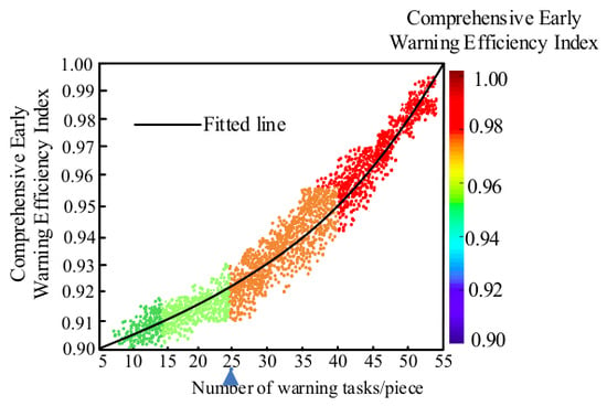
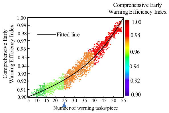
Taking the measured data set of rainfall debris flow in the study area for many years as the test sample, the sample covers the high-, medium-, and low-debris-flow-prone areas divided in Table 4, and includes all three types of rainfall conditions: short duration 3 h rainstorm, medium duration 7 h continuous rainfall, and long duration ≥ 14 h continuous rainfall. Using the number of historical disaster samples as the grouping gradient (5–55 groups), each sample corresponds to an independent warning task evaluation. It should be noted that the “5–55 sets of samples” used for performance testing here are independent and do not overlap with the 27 sets of samples used for CGWO offline calibration in Section 2.2.1. The test samples for each sample interval are sourced from independent monitoring events that did not participate in calibration during the rainy season of 2024–2025 in the study area (a total of 55 independent test events were obtained), to ensure that performance evaluation is not affected by the leakage of training data information. To objectively quantify the effect of threshold optimization, this article adopts the comprehensive warning energy efficiency index (CWEEI) as the evaluation index. The calculation formula for the index is: CWEEI = 0.4 × (1 − false alarm rate) + 0.4 × (1 − missed alarm rate) + 0.2 × dynamic threshold matching accuracy. The matching accuracy is graded based on the relative error between the model output threshold and the measured historical disaster-critical rainfall (relative error ≤ 5% is calculated as 1.0, 5~10% is calculated as 0.8, 10~15% is calculated as 0.6, >15% is calculated as 0). The three weights are determined according to the priority principle of equal importance of false alarms and missed alarms in early warning business, followed by threshold accuracy. The index value range is 0.90~1.00. The closer the value is to 1, the better the warning effect of the CGWO-IMRC threshold optimization method in this article. The test results are shown in Figure 5. To quantify the convergence and stability of the model under different levels of sample accumulation, this study constructed multiple independent testing scenarios within the CGWO-IMRC complete framework, gradually expanding from 5 to 55 calibration sample sizes. Among them, the 5- to 27-group scenarios were constructed by randomly sub-sampling from the 27 calibration samples to simulate different data accumulation stages during the calibration process (these are not independent test sets but are used to assess convergence behavior). The 28- to 55-group scenarios were formed by adding the 20 independent historical events from Table 3 that do not overlap with the calibration sample year and have independent rainfall parameters (also expanded proportionally according to partitioning). Cross-validation within each sample interval was independently performed using a 5-fold stratification, with a training/validation ratio of 4:1 for each fold. To quantify the convergence and stability of the model at different levels of sample size accumulation, 55 test samples were divided into four intervals (5–15, 16–25, 26–40, 41–55 groups) according to the sample size gradient. Within each interval, independent five-fold cross-validation was conducted, and the performance indicators are shown in Table 6.

Figure 5. Comprehensive warning energy efficiency index test results.

Table 6. Five-fold cross-validation performance metrics of CGWO-IMRC at different sample sizes.

Sample Size Range	Mean CWEEI (Full Training)	Mean CWEEI (5-Fold CV)	Std. Dev. of CV Folds	Max-Min Range of CV Folds	95% Prediction Interval Width (Based on CV Validation Set CWEEI Distribution)
5–15 groups	0.924–0.951	0.918–0.945	0.023–0.028	0.031–0.042	±0.045–± 0.055
16–25 groups	0.952–0.968	0.948–0.964	0.015–0.020	0.020–0.028	±0.030–± 0.040
26–40 groups	0.969–0.982	0.966–0.980	0.010–0.014	0.013–0.019	±0.020–± 0.028
41–55 groups	0.983–0.990	0.981–0.988	0.006–0.009	0.008–0.012	±0.012–± 0.015

In Figure 5, the horizontal axis represents the number of historical disaster sample groups (5–55 groups), and the vertical axis represents the comprehensive warning energy efficiency index CWEEI; the scatter points represent the measured energy efficiency values of each independent warning task, and the solid line is the logarithmic fitting curve. The fitting equation is CWEEI = 0.872 + 0.036·ln (N) (N is the number of sample groups, R² = 0.97, p < 0.001). The gray band area represents the 95% confidence band of the fitted curve, which is calculated based on the standard error of the logarithmic fitting parameters and reflects the statistical credibility of the parameter estimation of the fitting equation, rather than the prediction interval of a single warning task CWEEI. The narrowing trend of this confidence band only indicates that as the sample size increases, the fitting parameter estimation becomes more stable, and it is not directly used to evaluate the dispersion of single warning effectiveness. The testing procedure is as follows: samples are randomly selected in layers according to the prone areas (high/medium/low) and rainfall conditions (short/medium/long duration), and the proportion of samples in each layer is consistent with the actual frequency of disasters in Table 4. Each sample group independently runs the CGWO-IMRC model to complete threshold calculation and warning judgment, and then calculates the current CWEEI according to the above formula. Repeat the process to obtain the scatter distribution of the entire sample. All CWEEI values in Table 6 are the arithmetic means and their ranges of variation in CWEEI on five validation sets after independently performing 5-fold cross-validation within each sample size interval. The CWEEI calculation method on each validation set is consistent with the full sample test in Figure 5. There is no overlap between the data of each fold, ensuring the independence and unbiasedness of the verification results. At the same time, the “95% prediction interval width” for each principal interval is calculated based on the sample standard deviation of the CWEEI values of the five validation sets in the 5-fold cross-validation within that interval. The specific formula is: width = ± t_0.025(4) × (standard deviation/√5), where t_0.025(4) is the critical value of the t-distribution (2.776) at the 95% confidence level and degree of freedom 4. This interval represents that if a new set of independent test samples is randomly selected under the same geological zoning and rainfall conditions, there is a 95% probability that the CWEEI output by the model will fall within the range of “50% CV mean within this interval ± this width”. Therefore, this metric belongs to the prediction interval, rather than the Confidence Interval for estimating model parameters.

From the analysis of Figure 5 and Table 6, it can be seen that as the number of historical disaster samples (warning tasks) increases from 5 to 55, the comprehensive warning energy efficiency index continues to steadily rise, and all sample scatter points synchronously rise along the fitting curve without any accuracy decay. The results of the five-fold cross-validation are consistent with the training trend of the entire sample in each sample interval: in the low sample size stage (5~15 groups), the mean CWEEI on the five-fold validation set is 0.918~0.945, the standard deviation between each fold is about 0.023~0.028, and the range is about 0.031~0.042. The 95% predicted interval width calculated based on the CWEEI distribution of the validation set is about ± 0.045~± 0.055, reflecting the strong sensitivity of threshold correction to individual disaster samples under small sample conditions. However, the fluctuations between each fold of the cross-validation are still within an acceptable range, and no specific folds show abnormally low values, indicating that the model does not rely heavily on a specific data partition; when the sample size increases to more than 25 groups, the mean of the 5-fold CV is 0.948–0.964, the standard deviation narrows to 0.015–0.020, the width of the 95% prediction interval is compressed to ±0.030~±0.040, and the scatter tends to be concentrated; when the final sample covers all operating conditions (41~55 groups), the mean of the 5-fold CV reaches 0.981~0.988, the standard deviation drops to 0.006~0.009, the width of the 95% prediction interval narrows to ±0.012~±0.015, the energy efficiency index remains stable at 0.98~0.99, and the range between each fold does not exceed 0.012, indicating that the statistical convergence and stability of the model are significantly enhanced with data accumulation. The cross-validation results are highly consistent with the full sample training curve (0.98~0.99) in Figure 4, further verifying that the CGWO-IMRC method does not overfit in limited samples and its generalization performance is reliable. The algorithm in this paper has dual adaptive optimization capabilities: CGWO realizes spatial partition adaptation, and IMRC realizes rainfall time-series adaptation. For each new set of historical disaster data, the algorithm can autonomously correct the partition baseline rainfall and optimize the rainfall compensation amount. The more comprehensive the sample coverage, the more the threshold fits the actual disaster-causing pattern of the region, and the early warning performance improves in sync. This fully reflects the core advantage of adaptive optimization that iterates and improves continuously with the accumulation of data. The sample fully covers all rainfall conditions in high-, medium-, and low-risk areas, and the comprehensive energy efficiency reaches 0.98~0.99. CGWO solves the problem of static threshold differences in different geological partitions, and IMRC solves the problem of dynamic threshold correction for different rainfall durations. The two work together to adapt to the disaster-causing patterns of multiple types of historical disasters, proving that the adaptive threshold optimization algorithm can adapt to the differentiated and dynamic debris flow rainfall initiation conditions of the watershed, and can provide a reliable quantitative standard for refined graded early warning.

To further verify the superiority of the CGWO-IMRC method proposed in this paper, the fixed I-D threshold method and the classical statistical threshold method were selected as comparison methods on the same test dataset. The average comprehensive warning energy efficiency index of each method was calculated under all rainfall conditions in high-, medium-, and low-prone areas. The quantitative comparison results are shown in Table 7.

Table 7. Quantitative comparison of comprehensive warning energy efficiency index for different methods.

Method	High Susceptibility Area	Medium Susceptibility Area	Low Susceptibility Area	Overall Mean
Fixed I-D Threshold Method	0.72	0.78	0.83	0.78
Classical Statistical Threshold Method	0.81	0.85	0.88	0.85
CGWO-IMRC (Proposed Method)	0.98	0.99	0.98	0.98

As shown in Table 7, the overall average energy efficiency of the fixed I-D threshold method is 0.78, which performs relatively well in low-risk areas (0.83), but has a significantly higher missed alarm rate in high-risk areas (0.72), reflecting that a single fixed threshold cannot adapt to the differentiated disaster sensitivity of different geological zones. The overall mean of the classical statistical threshold method is 0.85, with 0.88 in the lower-prone areas and 0.81 in the higher-prone areas. Although it is better than the fixed threshold method, the false alarm rate still significantly increases under medium- and long-duration rainfall conditions due to the lack of consideration for the cumulative effect of rainfall duration and differences in zoning source conditions. In contrast, the CGWO-IMRC method proposed in this article significantly outperforms the two comparison methods in terms of various susceptibility zones and overall mean values. The energy efficiency in high, medium, and low susceptibility zones reaches 0.98, 0.99, and 0.98, respectively, with an overall mean of 0.98, which is a relative improvement of 25.6% and 15.3% compared to the fixed I-D threshold method and classical statistical threshold method, respectively. The quantitative comparison results fully demonstrate that the spatial partition adaptation implemented by the CGWO algorithm and the rainfall timing adaptation implemented by the IMRC module have a synergistic effect, which can simultaneously overcome the dual shortcomings of traditional methods of one threshold matching the entire domain and ignoring temporal dynamics. It has significant and stable early warning performance advantages under complex geological rainfall coupling conditions.

4. Conclusions

This study proposes an adaptive warning threshold setting algorithm that combines Chaos Grey Wolf Optimization (CGWO) and Internal Model Repetitive Control (IMRC) to address the key bottleneck of fixed thresholds in the early warning of debris flow disasters in the Heishui River Mountain area of the Anning River Basin, which cannot adapt to geological zoning differences and the dynamic superposition effect of rainfall time series. This method uses CGWO offline optimization to obtain static benchmark thresholds for high, medium, and low susceptibility areas, and utilizes the IMRC module to dynamically compensate for the soil saturation and pore water pressure evolution process caused by real-time rainfall duration, achieving a dual-layer collaborative control of “spatial zoning calibration” and “time process tracking”. The experimental results show that the algorithm achieved a comprehensive early warning energy efficiency index (CWEEI) of 0.98–0.99 under complete operating conditions in 27 independent calibration samples and 20 historical event validations, which is a relative improvement of 25.6% and 15.3% compared to the fixed I-D threshold method and classical statistical threshold method, respectively. The statistical convergence continues to increase with the accumulation of samples. This study provides a transferable and iterative quantitative technology path for fine grading and early warning of debris flows in complex geological rainfall coupling areas, which has important theoretical value and practical significance for improving the pertinence and timeliness of disaster prevention and reduction decisions in mountainous areas.

References

- Khan, M.U.; Tian, S.; Chen, N.; Khan, T.A.; Khan, U.S.; Ahmad, A.; Alam, M.; Latif, K.; Nyirandayisabye, R. Understanding the formation mechanism of rainfall and snowmelt jointly induced Bicharh Nallah debris flow, North Pakistan. Environ. Earth Sci. 2025, 84, 86. [Google Scholar] [CrossRef] [Scilit]
- Yousefi, S.; Imaizumi, F.; Takayama, S. Spatial distribution and transport characteristics of debris flow sediment using high resolution UAV images in the Ohya debris flow fan. Geomorphology 2025, 469, 1–14. [Google Scholar] [CrossRef] [Scilit]
- Barla, M.; Aiassa, S.; Antolini, F.; Insana, A.; Gaudino, R.; Martella, G.R.; Pellegrini, S. A new real-time debris flow and snow avalanche detection system based on optical fiber sensing. Landslides 2025, 22, 1367–1382. [Google Scholar] [CrossRef] [Scilit]
- Li, Y.; Zhang, J.; Jarsve, K.T.; Ma, F.; Huang, Y.; Zhao, W.; Zhao, Y.; Meng, X.; Wang, M.; Li, G.; et al. Debris flow forecasting: Disastrous rainfall threshold matters. Landslides 2025, 22, 2461–2474. [Google Scholar] [CrossRef] [Scilit]
- Ikhsan, J.; Fuqaha, S.; Rahardjo, A.P.; Suharyanto, S. Machine Learning for Rainfall-Driven Debris Flow Prediction in Data-Scarce Volcanic Watersheds. Int. J. Saf. Secur. Eng. 2025, 15, 2379–2391. [Google Scholar] [CrossRef] [Scilit]
- Zhang, S.L.; Guo, X.J.; Li, Y. Uncertainty and Optimization of Statistical Model for Rainfall-Triggered Debris Flow Forecast. Mt. Res. 2025, 43, 438–452. [Google Scholar]
- Xu, J.; Zhang, X.J.; Peng, Y.M.; Shi, M.S. Simulation of Multi-source Icing Early Warning Based on Adaptive Weight Feature. Comput. Simul. 2025, 42, 564–569. [Google Scholar]
- Kiryukhin, A.V.; Sergeeva, A.V.; Usacheva, O.O. Modeling of the thermal-hydrodynamic and chemical regime of Geyser reservoir (Valley of Geyser, Kamchatka). Geothermics 2023, 115, 102808. [Google Scholar] [CrossRef] [Scilit]
- Wells, A.G.; Hawbaker, T.J.; Hiers, J.; Kean, J.; Rachel, A.; Steblein, P.F. Predicting burn severity for integration with post-fire debris-flow hazard assessment: A case study from the upper colorado river basin, USA. Int. J. Wildland Fire 2023, 32, 1315–1331. [Google Scholar] [CrossRef] [Scilit]
- Esposito, G.; Gariano, S.L.; Masi, R.; Alfano, S.; Giannatiempo, G. Rainfall conditions leading to runoff-initiated post-fire debris flows in Campania, Southern Italy. Geomorphology 2023, 423, 108557. [Google Scholar] [CrossRef] [Scilit]
- Rabiei, M.; Fartash, M.; Nazari, S. A hybrid optimization approach for graph embedding: Leveraging Node2Vec and grey wolf optimization. J. Supercomput. 2025, 81, 514, Correction in J. Supercomput. 2025, 81, 650. [Google Scholar] [CrossRef] [Scilit]
- Ahmed, R.; Rangaiah, G.P.; Mahadzir, S.; Mirjalili, S.; Hassan, M.H.; Kamel, S. Memory, evolutionary operator, and local search based improved Grey Wolf Optimizer with linear population size reduction technique. Knowl.-Based Syst. 2023, 264, 110297. [Google Scholar] [CrossRef] [Scilit]
- Saplolu, K. Calibration of Linear Muskingum Model Coefficients and Coefficient Parameters Using Grey Wolf and Particle Swarm Optimization. Water Resour. Manag. 2025, 39, 999–1014. [Google Scholar] [CrossRef] [Scilit]
- Biswas, S.; Maiti, B.; Singh, G.; Mirjalili, S.; Simic, V.; Pamucar, D. An innovative hybrid method combining grey wolf and marine predator optimization techniques for global and constrained problem-solving. J. Supercomput. 2025, 81, 917. [Google Scholar] [CrossRef] [Scilit]
- Golanbari, B.; Mardani, A.; Valizadeh, M.; Farhadi, N. Hybrid grey wolf optimizer-ANN for predicting wheel energy consumption in off-road vehicles and enhancing resource management. J. Terramechanics 2025, 119, 101067. [Google Scholar] [CrossRef] [Scilit]
- Thomas, M.A.; Lindsay, D.N.; Cavagnaro, D.B.; Kean, J.W.; Mccoy, S.W.; Graber, A.P. The Rainfall Intensity-Duration Control of Debris Flows After Wildfire. Geophys. Res. Lett. 2023, 50, e2023GL103645. [Google Scholar] [CrossRef] [Scilit]
- Mondal, R.; Dey, J. Fractional order internal model control of non-minimum phase and time-delayed plants. Asian J. Control 2023, 25, 3208–3229. [Google Scholar] [CrossRef] [Scilit]
- Kovács, A.; Vajk, I. Internal Model-Based Robust Path-Following Control for Autonomous Vehicles. Int. J. Automot. Technol. 2024, 25, 249–260. [Google Scholar] [CrossRef] [Scilit]
- Aryan, P.; Raja, G.L.; Vilanova, R. Equilibrium optimiser tuned frequency-shifted internal model control proportional-derivative decoupled dual-loop design for industrial plants followed by experimental validation. Int. J. Syst. Sci. 2024, 55, 2874–2896. [Google Scholar] [CrossRef] [Scilit]
- Galuppini, G.; Creaco, E.; Magni, L. Real-Time Pressure Control in Water Distribution Networks: Stability Guarantees via Gain-Scheduled Internal Model Control. IEEE Trans. Control Syst. Technol. 2024, 32, 731–743. [Google Scholar] [CrossRef] [Scilit]
Disclaimer/Publisher’s Note: The statements, opinions and data contained in all publications are solely those of the individual author(s) and contributor(s) and not of MDPI and/or the editor(s). MDPI and/or the editor(s) disclaim responsibility for any injury to people or property resulting from any ideas, methods, instructions or products referred to in the content. |
© 2026 by the authors. Licensee MDPI, Basel, Switzerland. This article is an open access article distributed under the terms and conditions of the Creative Commons Attribution (CC BY) license.