Prediction of Chl-a Concentration Based on Time-Lag Effects and LSTM Model: A Case Study of Wuli Lake

Abstract

Accurately predicting chlorophyll-a (Chl-a) concentration in lakes is critical for water-quality management and ecological protection. This study investigated whether the time-lagged effects of meteorological factors improve Chl-a prediction at one fixed station in Wuli Lake, using hourly observations from May to October 2023. Rank correlations, prior process knowledge and multicollinearity diagnostics were used to identify a nonredundant driver set before interpreting meteorological lags. Cross-wavelet transform and wavelet cross-correlation analyses identified sub-daily lag associations: phase-derived lags were approximately 7.48 ± 4.03 h for air temperature and 6.44 ± 0.84 h for wind speed, while the corresponding cross-correlation maxima occurred at 9 h and 8 h. Incorporating lag-aligned meteorological inputs into a long short-term memory (LSTM) model for 1 h-ahead prediction increased the mean R² across 100 training runs per scheme from 0.719 to 0.809 and reduced MAE and prediction-bias dispersion; RMSE remained approximately 0.0017 mg/L at the reported precision. Factorial ablations separately evaluated temperature and wind alignment and showed that their gains depend on the input-variable set. These descriptive results suggest that wavelet-derived temporal alignment may improve the accuracy of hourly Chl-a prediction and provide a basis for prospective bloom-warning systems.

1. Introduction

Cyanobacterial-bloom prediction is needed because management decisions depend on when biomass will increase, not only on whether a lake is eutrophic. Across freshwater systems, bloom development reflects interactions among nutrient supply, thermal conditions, light availability and hydrodynamics; consequently, nutrient enrichment alone cannot explain the timing or intensity of every event [1,2,3]. Blooms in low-nutrient lakes further challenge a uniform nutrient-based prediction rule [4]. Chlorophyll-a (Chl-a) provides a practical indicator of changing algal biomass, but biomass forecasts should be distinguished from predictions of cyanobacterial dominance, visible surface scums or toxin risk [5]. For short-term water-quality monitoring, the relevant question is therefore whether routinely observed environmental information improves prediction of future Chl-a beyond the information already contained in its recent history.

The timing of environmental information is especially important in shallow lakes. Light supplies energy for photosynthesis, whereas underwater exposure depends on attenuation, mixing and the position of cells in the water column. Temperature regulates physiological conditions and interacts with the seasonal light regime; wind simultaneously affects mixing, sediment suspension and biomass redistribution [2,3,6]. A rapid change in measured Chl-a can therefore reflect transport or optical and physiological responses as well as net population growth. These interacting processes make a contemporaneous correlation insufficient to identify either a unique mechanism or the hour at which a driver becomes useful for prediction. They also mean that temperature or turbidity cannot simply be treated as a measurement of irradiance.

Predictor selection and response timing address related but distinct uncertainties. Multivariable driver analyses in Taihu provide a basis for screening candidate variables, yet ecological relevance can vary among lake regions and states [7]. At a fixed station, shared seasonal variation and correlations among water-quality indicators may produce strong marginal associations without independent information; collinearity then complicates attribution [8]. Conversely, a meteorological variable with weak zero-lag association may still carry delayed information. Forecasting evidence also shows that variables associated with historical cyanobacterial density need not improve short-horizon forecasts beyond a recent-density baseline [9]. Thus, selecting drivers, estimating their lags and demonstrating their incremental predictive value require separate tests rather than inference from association strength alone.

Response lags are not constants that can be transferred unchanged between systems. Evidence from reservoirs and regulated rivers indicates that resolved delays depend on water-column stability, nutrient conditions, hydrological setting and sampling resolution [10,11]. Wavelet methods can examine how common variability and phase relationships change through time and across periods [12,13], making them useful for high-frequency observations with nonstationary signals. However, common wavelet power and phase do not establish causality, and a phase-derived offset is not automatically the best predictive input shift. The unresolved issue for hourly lake monitoring is whether explicitly aligning meteorological histories with the observed response timing adds information to a recurrent forecasting model.

Existing prediction approaches address complementary parts of this problem. Wavelet-based deep learning represents variability at multiple temporal scales, while hydrodynamic–LSTM coupling supplies information about physical transport [14,15]. Recurrent forecasts, machine learning soft sensors and alternative regressors demonstrate several ways to exploit environmental records [16,17,18]; Bayesian-network forecasts additionally show the value of testing performance when covariates are unavailable [19]. These advances make another application of LSTM, or a combination of wavelets and LSTM, insufficient by itself to establish novelty. Moreover, forecast performance depends on the target, horizon, observations and evaluation design: prediction errors, alarm metrics and skill relative to recent observations answer different questions [9,16]. For the present application, separate temperature and wind alignment tests and comparisons between full and screened input sets are needed to establish the scope of any gain.

The remaining question is whether meteorological lag alignment adds predictive information and whether its contribution depends on the other predictors supplied to the model. This study addresses that question using hourly Chl-a, water-quality and meteorological records from one fixed station in Wuli Lake during May–October 2023. Rank-based association and redundancy screening are linked to wavelet characterization of sub-daily temperature and wind timing, followed by LSTM evaluation for 1 h-ahead Chl-a prediction. Factorial tests compare unshifted, temperature-aligned, wind-aligned and jointly aligned inputs under full and screened predictor sets. The specific contribution is to distinguish the separate and joint predictive value of the two lag alignments and assess its dependence on predictor selection. This evaluation informs the choice of meteorological input windows and predictor combinations for hourly monitoring forecasts. The contribution is this explicit connection between driver screening, temporal association and conditional prediction gain, rather than a new neural network architecture or a first use of wavelets with LSTM.

2. Materials and Methods

2.1. Study Area, Hydrology, and Monitoring Design

Wuli Lake is located in Wuxi City, Jiangsu Province, China, and forms a relatively enclosed northern bay connected to Meiliang Bay of Lake Taihu (approximately 31°30′–31°33′ N, 120°13′–120°17′ E). The region has a subtropical monsoon climate, with warm, humid summers and cool winters. Wuli Lake is a shallow, polymictic urban lake. Published morphometric data report a surface area of approximately 6.4 km², a mean depth of 1.6 m, and a maximum depth of 2.6 m [20]. The corresponding nominal water volume, calculated as surface area multiplied by mean depth, is approximately 1.02 × 10⁷ m³.

Hydrologically, Wuli Lake receives runoff from surrounding urban tributaries and is influenced by regulated water diversion. Its principal through-flow routes extend from the western lake toward eastern and southern outlets. Hydrodynamic modeling has shown that diversion discharge, outlet configuration, wind forcing, and bed roughness jointly control circulation and create spatially heterogeneous exchange, including weakly flushed or recirculating zones [21]. Using the nominal lake volume above and the representative diversion discharge of 50 m³/s reported for the engineering system [21], the ideal complete-mixing water-exchange period (τ = V/Q) is approximately 2.4 days. This value is an engineering-scale estimate rather than a measured local residence time during the monitoring period; actual water age can be longer in poorly connected zones. These conditions are relevant to algal growth: shallow water heats rapidly, weak exchange favors nutrient and algal-cell retention, and wind can mix the entire water column, redistribute algae, and resuspend nutrient-rich sediment [6,20,21]. Consequently, meteorological forcing may first alter local thermal and mixing conditions and only later produce a measurable Chl-a response.

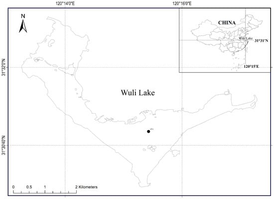
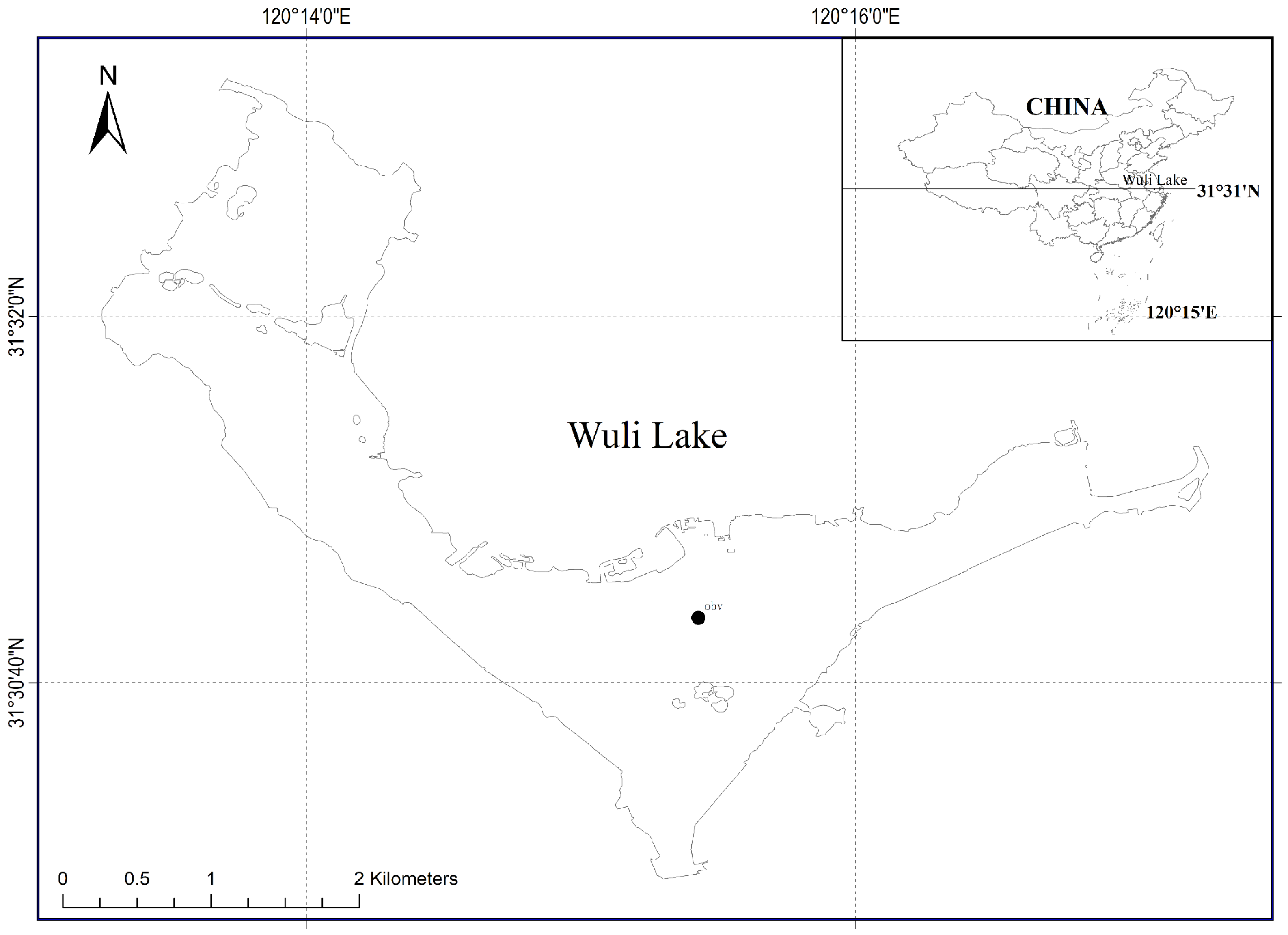
The monitoring data were provided by the Jiangsu Provincial Environmental Monitoring Center and were collected at one fixed high-frequency station, coded OBV (approximately 31°30′55″ N, 120°15′25″ E; Figure 1). The analysis covered 184 consecutive days from 00:00 on 1 May to 23:00 on 31 October 2023. The analysis dataset had a temporal resolution of 1 h, corresponding to a maximum of 4416 hourly timestamps before alignment and quality control. Variables comprised Chl-a, ammonium nitrogen, total phosphorus, total nitrogen, water temperature, pH, dissolved oxygen, electrical conductivity, turbidity, algal density, air temperature, and wind speed. All variables were aligned by timestamp, and only complete hourly records were used in the wavelet and LSTM analyses. Because this study used a single fixed station, the results characterize temporal predictability at OBV rather than spatial variability across Wuli Lake.

Figure 1. Location of Wuli Lake and the single fixed high-frequency monitoring station (OBV).

2.2. Overall Research Workflow

The analysis links four stages: (i) hourly alignment and complete-record selection for the 12 monitored variables; (ii) CWT characterization of periodicity and XWT examination of common power and phase between Chl-a and each meteorological variable; (iii) phase-to-time conversion and a complementary wavelet cross-correlation lag scan; and (iv) a comparison of LSTM forecasts using unshifted and lag-aligned meteorological inputs. The common prediction target is Chl-a one hour beyond the last nominal input time. The wavelet analyses characterize temporal associations; the LSTM comparison evaluates their predictive use.

2.3. Rank Correlation and Driver Screening

Spearman rank correlation was used to assess monotonic associations without assuming normally distributed concentrations [22]. We calculated rho(X,Y) as the Pearson correlation of average ranks, accounting for tied observations. Chl-a was the response, and the other 11 contemporaneous variables were candidate explanatory variables; historical Chl-a was reserved for forecasting and was not ranked as an environmental driver. Screening used 2177 fitting-period final input contexts, each at t − 1, drawn from the common eligible forecasting windows defined in Section 2.7. The response for screening was Chl-a(t − 1), not the future forecast target Chl-a(t). Test-period values and prediction errors were not used to select variables. Uncertainty in the marginal rank correlations was summarized using 500 day-cluster bootstrap resamples (seed 20261010; 113 observed day clusters), preserving within-day observations and gaps. The percentile intervals describe sample variability and do not prove causal effects or account for all dependence beyond one day.

Candidate relevance was assessed by combining absolute Chl-a rank association with process knowledge. Total phosphorus was retained as a nutrient-supply indicator, temperature was retained as external thermal forcing, and wind speed was retained as a mixing and transport driver [2,6,7]. Temperature and wind were therefore protected from removal solely on the basis of weak concurrent association, which would prejudge a delayed-response hypothesis. Algal density represents a biomass-related state indicator, not an exogenous forcing. Among predictor pairs with |rho| ≥ 0.80, one variable was removed, prioritizing the protected variables and otherwise retaining the variable with the stronger absolute Chl-a association. Pairwise screening was followed by iterative VIF assessment on standardized environmental predictors: VIFj = 1/(1 − Rj²), where predictor j was regressed on the others with an intercept. The unprotected predictor with the largest VIF was removed until all retained VIF values were ≤5. Thresholds are operational diagnostics of redundancy, not universal biological cutoffs [8].

To distinguish marginal association from conditional relevance, partial Spearman coefficients were calculated for retained variables by correlating residuals of ranked Chl-a and each ranked predictor after regressing both on the other retained ranked predictors. Absolute marginal rho supplies a descriptive association ordering; the partial coefficient supplies a conditional association check. Neither is a complete nonlinear importance measure. The screened set is used in the reduced-input ablations, while the full-input model remains a reference for the originally evaluated predictor configuration.

2.4. Wavelet Analysis

2.4.1. Continuous Wavelet Transform

Continuous wavelet transform (CWT) resolves a nonstationary series in time and scale. Torrence and Compo [12] provide the methodological basis for wavelet power, significance and edge-effect interpretation. Here, CWT is used to examine transient periodicities in hourly Chl-a, air temperature and wind speed. For a series x(t), the transform is defined as:

$$W_{x;\varphi }\left(\tau ,s\right)={\int }_{-\infty }^{\infty }x\left(t\right){\displaystyle \frac{1}{\sqrt{\left|s\right|}}}\varphi *\left({\displaystyle \frac{t-\tau }{s}}\right)\mathit{dt}$$

(1)

In the formula, τ is the translation parameter, which allows obtaining signals in different time domains. s is the scale parameter, used to obtain information at different scales by expanding or contracting the wavelet width.${\displaystyle \frac{1}{\sqrt{\left|s\right|}}}\varphi *\left({\displaystyle \frac{t-\tau }{s}}\right)$ is the wavelet function, and * denotes the complex conjugate. The edge artifacts generated after the continuous wavelet transform occur because the mother wavelet cannot be completely localized in time. Therefore, the cone of influence is introduced to represent the region where errors in the wavelet power spectrum occur.

2.4.2. Cross-Wavelet Transform

Cross-wavelet transform (XWT) combines the complex CWT coefficients of two series. It can reflect the resonance period and phase relationship of two time series x_t and y_t across different time scales [13]. The cross-wavelet power is defined as

$$C_t\left(s\right)=\left|W_t^{\mathit{xy}}\left(s\right)\right|=\left|W_t^x\left(s\right)W_t^{y*}\left(s\right)\right|$$

(2)

The phase angle spectrum (A_t) is used to describe the local relative phase between two time series x_t and y_t. Its formula is given by

$$A_t\left(s\right)={\mathit{tan}}^{-1}\left\{{\displaystyle \frac{\mathit{lm}\left[W_t^{\mathit{xy}}\left(s\right)\right]}{\mathit{Re}\left[W_t^{\mathit{xy}}\left(s\right)\right]}}\right\}$$

(3)

In this formula, $\mathit{lm}\left[w_t^{\mathit{xy}}\left(s\right)\right]$ is the imaginary part of the cross-wavelet spectrum, and $\mathit{Re}\left[W_t^{\mathit{xy}}\left(s\right)\right]$ is the real part of the cross-wavelet spectrum. Unlike an overall lagged correlation, wavelet analysis localizes relationships in time and period. XWT describes common power and phase, not normalized coherence. A phase φ at period P corresponds to an offset φP/(2π), with the sign determined by series order; phase must retain its quadrant. The lag alignment and LSTM construction are described in Section 2.5 and Section 2.6.

2.5. Lag Estimation and Input Alignment

For each meteorological series, a local phase offset φ at period P is converted to a time offset φP/(2π). Phase-derived estimates and cross-correlation peaks are reported separately because they summarize different features of the signals. The former describe phase offsets in selected time–period regions; the latter identify the shift at which the reported wavelet cross-correlation coefficient reaches its maximum. In the available analysis, the temperature and wind-speed cross-correlation peaks occur at 9 h and 8 h, respectively (Section 3.5); these values are not interchangeable with the mean phase-derived offsets in Table 1.

Table 1. Time-lag analysis of Chl-a concentration in Wuli Lake with temperature and wind speed.

Chl-a Concentration	Cross-Phase Angle/rad	Time-Lag /h
Temperature	2.0274 ± 1.0187	7.4816 ± 4.0312
Wind speed	1.7747 ± 0.1360	6.4392 ± 0.8386

Writing the air-temperature and wind-speed offsets as ℓT and ℓW, lag alignment replaces the meteorological inputs at nominal hour u by T(u − ℓT) and W(u − ℓW). The other variables retain their original timestamps. A 10-step input at nominal times t − 10, …, t − 1 is used to predict Chl-a at t. Thus, alignment changes the meteorological history supplied to the model; it does not increase the forecast horizon. If ℓT = 9 h and ℓW = 8 h were used, the temperature observations span t − 19, …, t – 10, and the wind observations span t − 18, …, t − 9. The actual implemented offsets must therefore be distinguished from the nominal 10 h sequence length.

2.6. LSTM Construction and Evaluation

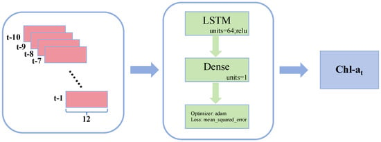
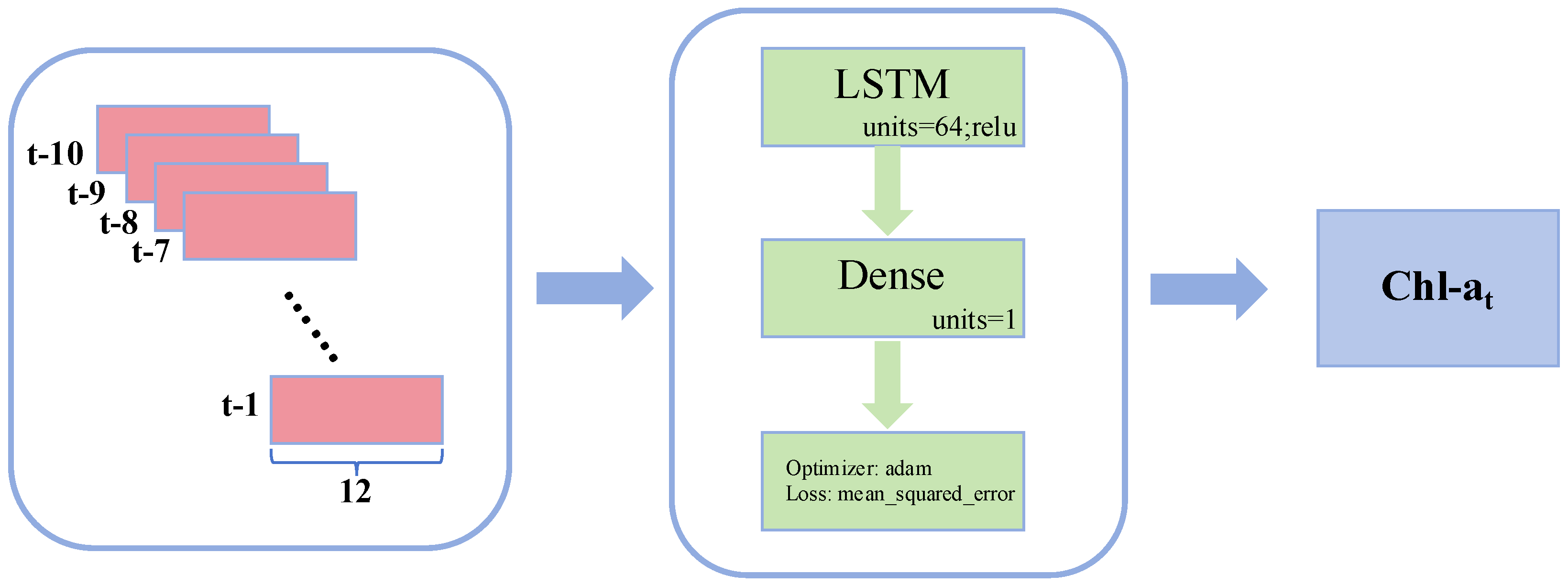
The LSTM implementation and input/output structure are shown in Figure 2. A recurrent model is a reasonable test bed because the input consists of ordered hourly multivariable sequences, and prior bloom studies have used LSTM [14,15,16]. This choice provides a fixed architecture for evaluating lag alignment; it does not establish that LSTM is better than Random Forest or TCN for the present dataset.

Figure 2. Wuli Lake Chl-a concentration prediction framework based on the LSTM model.

(1)

Input variables and sequence construction: The full-input reference model used 12 variables: Chl-a, ammonium nitrogen, total phosphorus, total nitrogen, water temperature, pH, dissolved oxygen, electrical conductivity, turbidity, air temperature, algal density, and wind speed. Each input sample contained a 10 h look-back sequence of consecutive hourly observations. With a 1 h sliding stride, one new supervised-learning sample was generated for each eligible hourly timestamp; the monitoring frequency was therefore 1 h, not 10 h. In the lag-aware model, air temperature and wind speed were shifted according to the response window identified by the wavelet analyses before the sequences were constructed. In Figure 2, inputs at t − 10, …, t − 1 predict Chl-a at t, corresponding to a 1 h-ahead forecast. The meteorological lag is an input offset, not the forecast horizon.

(2)

Dataset split: The time-ordered sequence was divided chronologically, with the first 80% used for training and the final 20% used for testing. Temporal order was retained, and the data were not randomly shuffled, preserving the chronological order of the training and test records.

(3)

Deep Learning Model: The middle section contains the LSTM model, which includes three core modules:

•

LSTM Layer: A unidirectional LSTM layer with 64 neurons and ReLU activation function, used to capture time-series patterns.

•

Dense Layer: Used to generate the model’s output value, i.e., the predicted Chl-a concentration.

•

Optimizer and Loss Function: The Adam optimizer is used to update the network parameters, and the mean squared error (MSE) loss function is chosen to measure the difference between predicted and actual values.

(4)

Output: The model ultimately outputs the predicted Chl-a concentration value. For observations y_i and predictions ŷ_i on n common test targets, R² = 1 − Σ(y_i − ŷ_i)²/Σ(y_i − ȳ)², RMSE = [Σ(y_i − ŷ_i)²/n]¹ᐟ², and MAE = Σ|y_i − ŷ_i|/n; positive bias is defined as ŷ_i − y_i.

Each input scheme was fitted 100 times to describe variability associated with initialization and optimization. The reported R², RMSE and MAE summarize predictive performance, while the time-series plots and bias distributions describe temporal agreement and residual spread. Repeated fits on one chronological split characterize training variability; they do not constitute 100 independent temporal validation datasets.

2.7. Factorial Ablation and Reproducible Training Protocol

The ablation design crosses two factors: a temperature offset of either 0 or 9 h and a wind-speed offset of either 0 or 8 h. This produces no alignment, temperature-only alignment, wind-only alignment and joint alignment. All four configurations are evaluated with both the full 12-input set and the screened seven-input set, which consists of historical Chl-a plus TP, TN, DO, T, AD and WS. The recurrent architecture, forecast target, eligible timestamps and training controls remain fixed within each input set. Removing a lag means removing its offset, not removing that meteorological variable. The full-input and screened-input blocks test whether alignment effects depend on covariate redundancy.

Separate contributions are measured by paired changes in test RMSE. For error Eij, i and j indicate temperature and wind alignment. Temperature contrasts are E00–E10 (alone) and E01−E11 (given wind); wind contrasts are E00–E01 (alone) and E10–E11 (given temperature). Positive differences indicate improvement. Metrics and paired differences are reported as means ± sample SD across five seeds; these repeats quantify training variability on one holdout period, not independent temporal validation. A previous-hour persistence forecast provides a reference. Fixed lag choices are taken from the wavelet results and are not optimized against test errors; their original estimation on the study record does not constitute training-only validation of optimal lags.

3. Results

3.1. Analysis of Seasonal Variation in Impact Factor

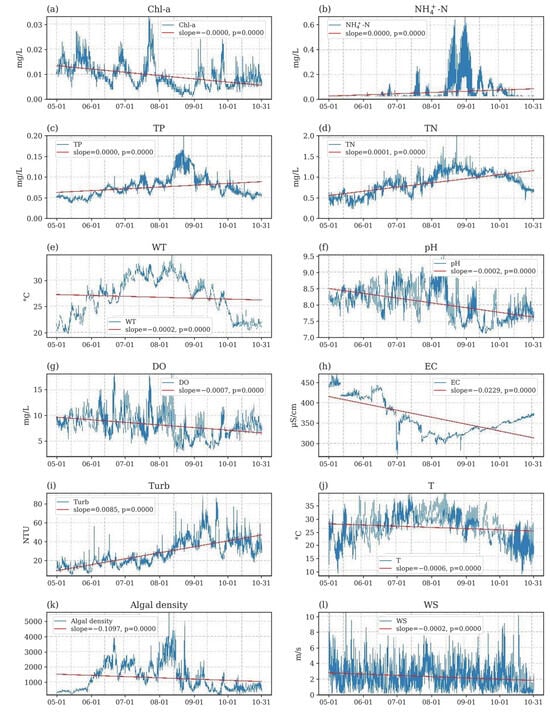
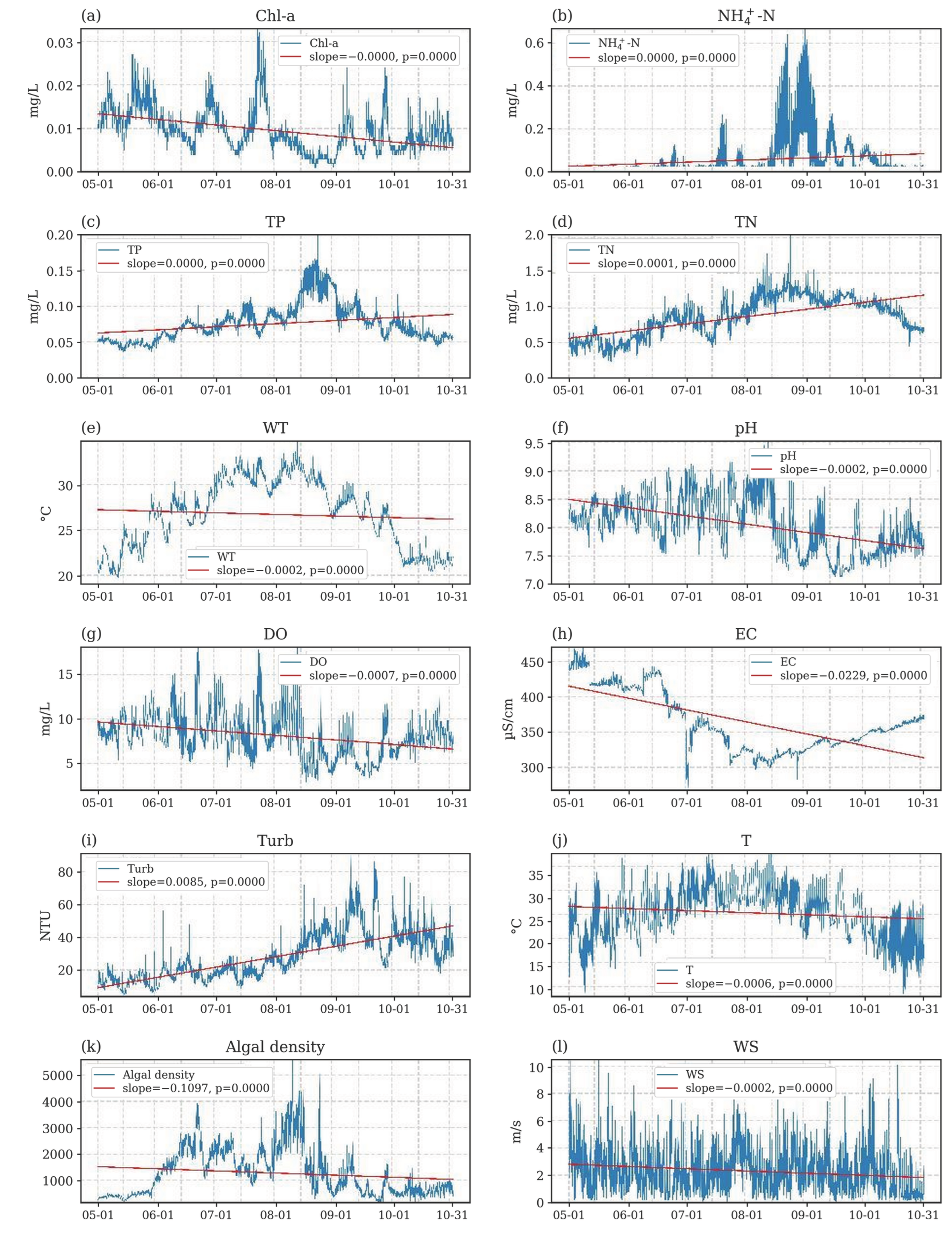
Figure 3 shows the hourly time series of Chl-a (a), ammonium nitrogen (b), total phosphorus (c), total nitrogen (d), water temperature (e), pH (f), dissolved oxygen (g), electrical conductivity (h), turbidity (i), air temperature (j), algal density (k), and wind speed (l) at station OBV from May to October 2023. Chl-a fluctuated strongly during the monitoring period and reached a maximum of 0.033 mg/L in August. Ammonium nitrogen, total phosphorus, total nitrogen, algal density, and water temperature also showed pronounced summer variation, although their peaks were not fully synchronous. These patterns are consistent with the combined influence of warm conditions, changing light availability, nutrient supply, hydrodynamic mixing, and biological activity; they should not be interpreted as evidence that any single factor independently controlled Chl-a.

Figure 3. The variation sequences of Chl-a (a), NH4⁺-N (b), TP (c), TN (d), WT (e), pH (f), DO (g), EC (h), Turb (i), T (j), Algal density (k), WS (l).

The pH value shows a downward trend from May to October, with the most rapid decline occurring in mid-August, which may have certain effects on the aquatic ecological environment. The variation in dissolved oxygen (DO) concentration is similar to that of pH, although this temporal association does not establish algal proliferation as its cause. In addition, air temperature rises toward summer and then declines, while wind speed remains variable.

3.2. Candidate Associations and Redundancy Screening

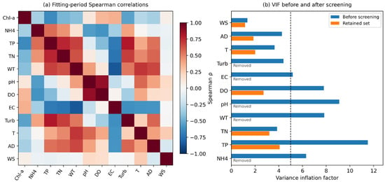
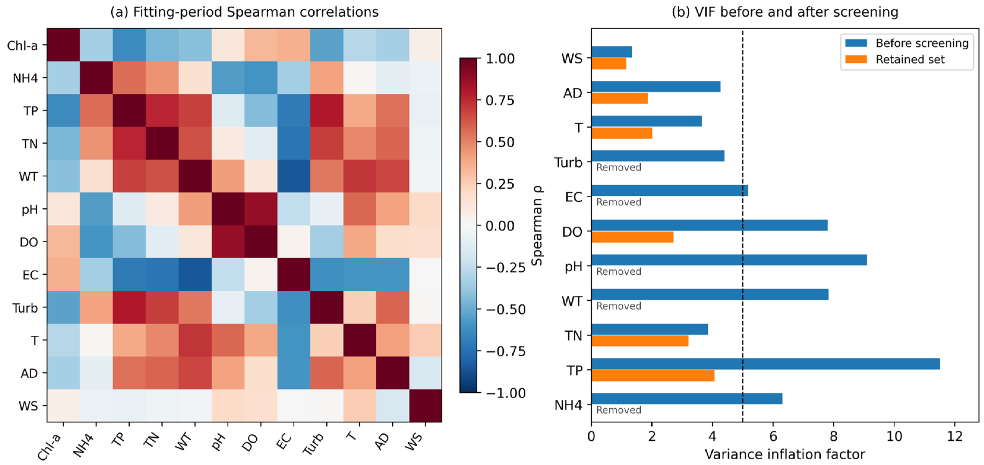
Figure 4a shows the concurrent Spearman correlation matrix. The marginal associations identify the strongest observed Chl-a relationships, while the partial coefficients reported below describe conditional associations. TP (rho = −0.635), turbidity (−0.533) and TN (−0.455) have the strongest marginal associations in the fitting data. Temperature has rho = −0.283, and wind speed has rho = 0.057; wind’s day-cluster interval includes zero. These values describe the observed season and sampling context. In particular, a negative nutrient–Chl-a association cannot be interpreted as evidence that nutrients inhibit algal growth: uptake, seasonal progression and common environmental variation can produce inverse contemporaneous relationships. Low concurrent wind correlation also does not rule out a delayed or nonlinear effect.

Figure 4. Correlation and collinearity screening. (a) Fitting-period Spearman matrix; (b) VIF before screening (blue) and for retained predictors (orange). The dashed line marks VIF = 5; removed predictors have no final VIF bar.

The strongest redundant pairs are pH–DO (|rho| = 0.882), WT–EC (0.849) and TP–turbidity (0.805). Pairwise screening removes pH, EC and turbidity, retaining stronger Chl-a associations or the protected nutrient indicator. Subsequent VIF screening removes WT and NH4, retaining temperature as the external thermal forcing and TP and TN as nutrient indicators. The final six environmental predictors are TP, TN, DO, T, AD and WS; their VIF values range from 1.154 to 4.069 (Figure 4b). Adding historical Chl-a produces seven forecasting inputs. These omissions remove overlapping columns in the screened model; they do not imply that water temperature, ammonium or turbidity are ecologically irrelevant.

After adjustment, TP retains the strongest absolute partial association (−0.277), followed by T (−0.172) and DO (0.156); TN, AD and WS have smaller partial coefficients (0.055, −0.041 and 0.037). Thus, marginal rankings do not transfer directly to independent explanatory importance. Temperature and wind remain the meteorological variables examined with wavelets because prior process knowledge and the delayed-response hypothesis justify assessing their timing. The next sections examine that timing rather than selecting them merely because of high zero-lag correlation.

3.3. Lag Response of Chlorophyll-a to Meteorological Factors

The growth of algae is influenced by the interaction of multiple physical, chemical, and biological factors, exhibiting complex nonlinear characteristics. Meteorological factors, especially temperature and wind speed, play a crucial role in regulating algae growth and concentration changes. In particular, in Wuli Lake, the concentration of chlorophyll-a (Chl-a) is not only directly affected by these factors but may also exhibit a lag effect, meaning that the influence of meteorological factors on Chl-a concentration may take some time to manifest. Therefore, a thorough investigation of the response relationship between Chl-a concentration and meteorological factors, especially their lag response characteristics, is essential for improving the accuracy of algae bloom predictions.

Temperature and wind speed were retained as external thermal and mixing drivers in the screening step. Their concurrent associations do not fully represent the timing of a Chl-a response. We therefore examined Chl-a, temperature and wind with wavelet methods to resolve variations across time and period before specifying input offsets for prediction.

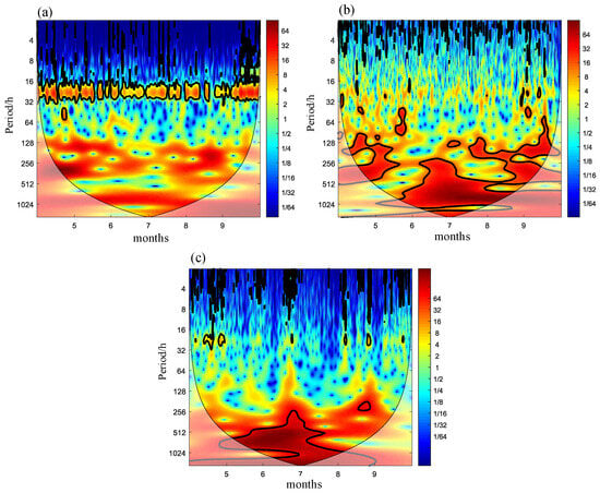
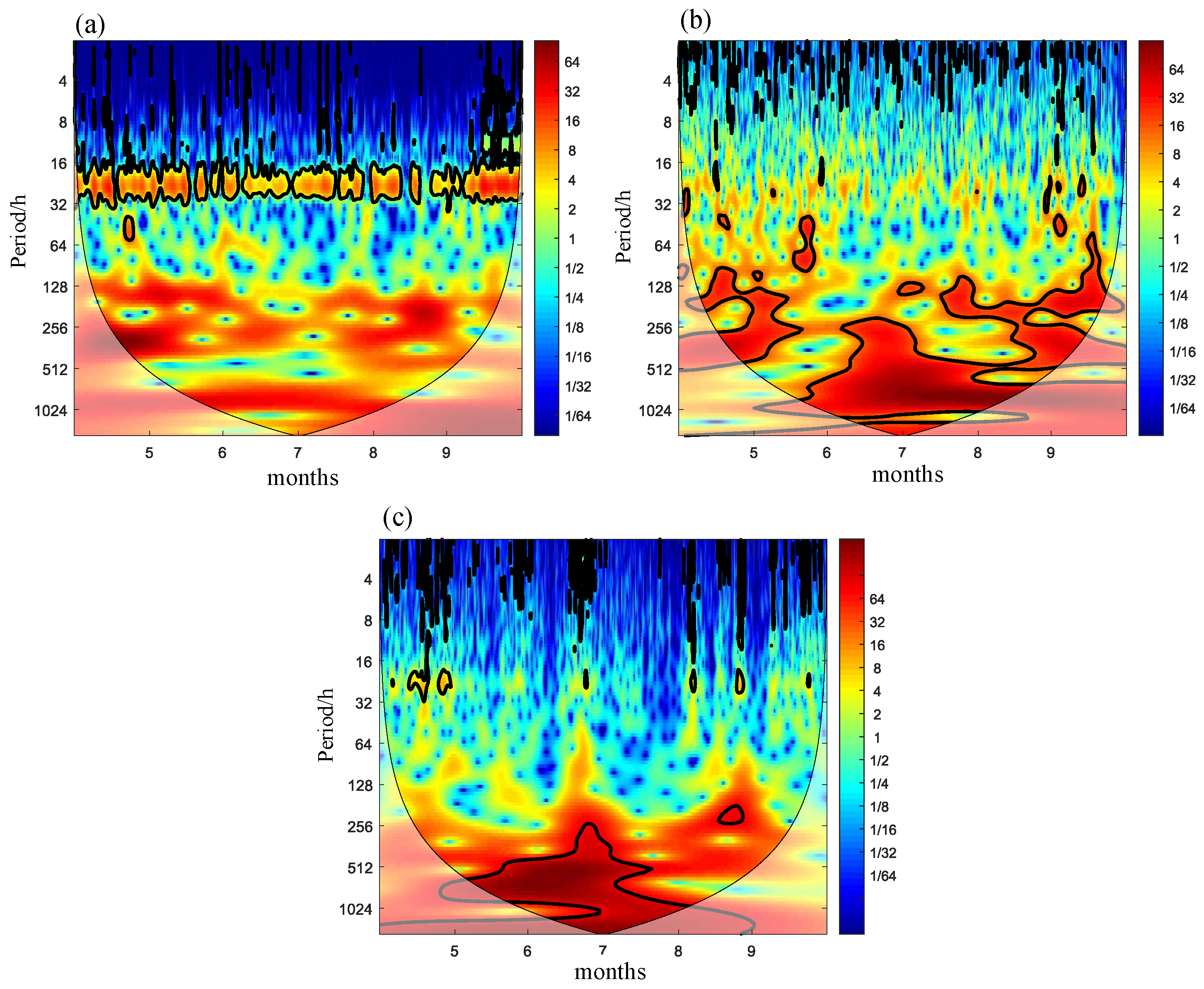
Figure 5 presents the continuous wavelet transform results for air temperature (a), wind speed (b), and Chl-a (c) at station OBV. The thick black contour denotes regions exceeding the 95% confidence level, the thin black curve denotes the cone of influence, and the shaded region indicates edge-affected estimates. As shown in Figure 5a, air temperature exhibits a significant oscillatory period in the 16–32 h range, with additional scattered oscillations near 16 h. The dominant periodicity of wind speed (Figure 5b) shifts seasonally: energy initially occurs mainly at 128–512 h, extends toward 512–1024 h between June and August, and returns toward 128–512 h from August to October.

Figure 5. The continuous wavelet transform of temperature (a), wind speed (b), and chlorophyll-a (c) in the Wuli Lake.

The periodic variation in Chl-a (Figure 5c) partly follows the wind-speed pattern, although several intervals between May and August and between August and October do not exceed the 95% confidence threshold. The shorter periodicity observed from June to August and the different timing of seasonal transitions likely reflect the combined influence of air temperature, wind-driven mixing, nutrient availability, and other unmeasured processes.

3.4. Phase Relationships Between Chl-a and Meteorological Factors

The growth of algae is regulated by a combination of various physical, chemical, and biological factors, and its dynamic changes exhibit significant nonlinear and complex characteristics. Meteorological factors (such as temperature, precipitation, and wind speed) play an important role in regulating algal growth and changes in chlorophyll-a (Chl-a) concentration, especially in shallow lake ecosystems. The variation in Chl-a concentration in Wuli Lake is not only directly driven by meteorological factors but may also exhibit significant time lag effects, reflecting the ecosystem’s response time to external environmental changes.

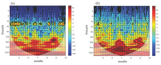
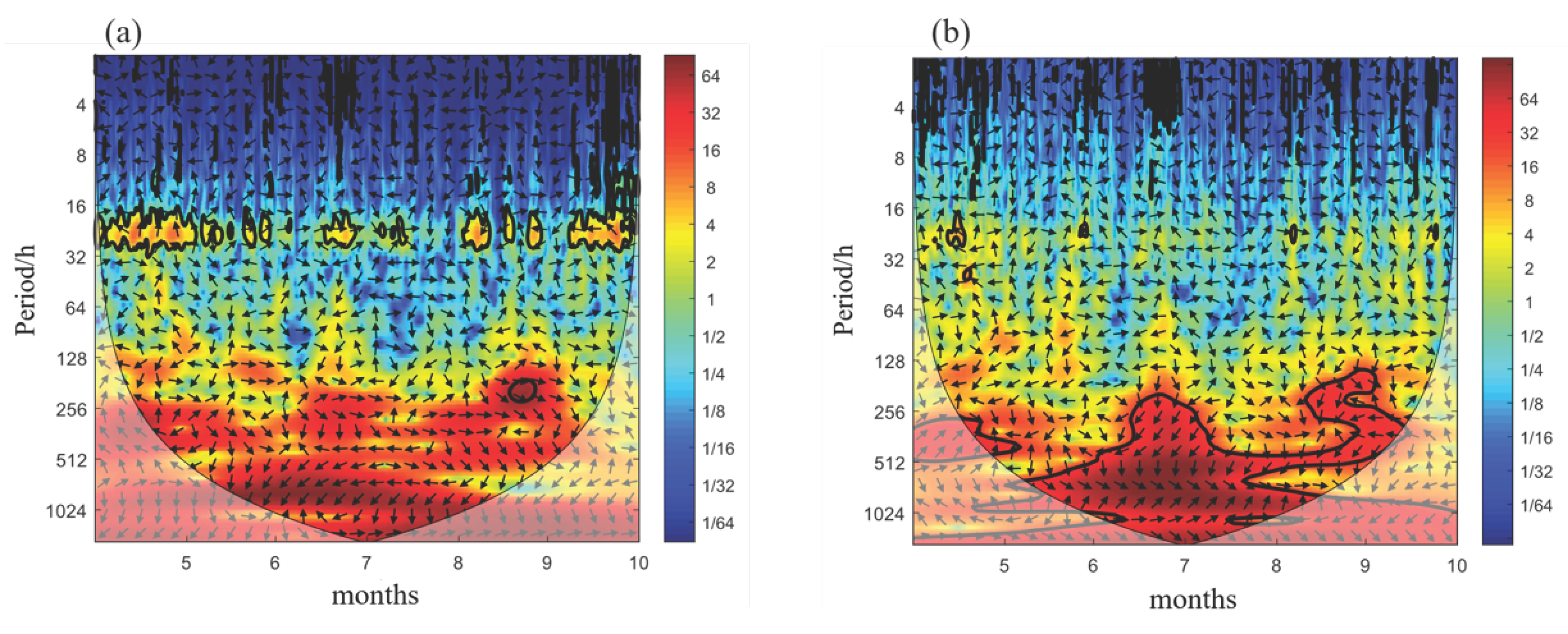
Figure 6 shows the cross-wavelet power and phase relationships between Chl-a and air temperature (a) and between Chl-a and wind speed (b). Air temperature exhibits significant common power with Chl-a mainly at intermediate periods (128–256 h), with additional energy at longer periods (512–1024 h). The Chl-a–wind relationship is more temporally variable, with common power concentrated mainly at 128–256 h from June to August and extending to longer periods from August to October. Phase arrows vary across time and period; their directions alone do not establish a consistent meteorological lead. Lag interpretation requires a defined period range, significance and edge mask, and verified phase convention.

Figure 6. The cross-wavelet transform between Chl-a concentration in Wuli Lake and temperature (a) and wind speed (b).

The periodic variations in Chl-a concentration show high consistency with the trends of meteorological factors. Particularly between June and August, significant oscillations of Chl-a concentration are concentrated in the 128–256 period range, which matches the fluctuations of wind speed and temperature. However, from August to October, although the periodic variation ranges of wind speed and temperature change, the response of Chl-a did not fully pass the 95% confidence interval test. This phenomenon may be related to the complexity of the synergistic effects of meteorological factors and could also be influenced by other non-meteorological factors (such as water nutrient concentration and light conditions). Overall, the observed associations suggest time-varying relationships between various meteorological factors and Chl-a concentration, providing important insights for understanding the algal dynamics in the Wuli Lake ecosystem.

3.5. Quantification of Meteorological Response Lags

Through phase spectrum analysis using cross-wavelet transform, we can further obtain specific time-lag analysis at different periods, with the results shown in Table 1.

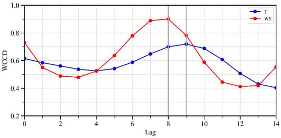
Based on the time-lag analysis using cross-wavelet transform, a complementary time-lag analysis between Chl-a concentration and temperature and wind speed was further conducted using wavelet cross-correlation, with the results shown in Figure 7. The wavelet cross-correlation between Chl-a concentration and temperature first decreases within the time-lag range of 0 to 4 h and then gradually increases, reaching a maximum value of 0.72 at 9 h. As the time lag further increases, the cross-correlation begins to decrease. The relationship between wind speed and Chl-a concentration exhibits a similar pattern, with the maximum cross-correlation value of 0.90 occurring at a time lag of 8 h.

Figure 7. Wavelet cross-correlation analysis between Chl-a concentration in Wuli Lake and temperature (blue line) and wind speed (red line). The lag is in hours; WCCD denotes the reported dimensionless wavelet cross-correlation coefficient.

In summary, Chl-a concentration exhibits a delayed response to temperature and wind speed changes of 9 h and 8 h, respectively, which is broadly similar in timescale to, but not identical to, the phase-derived estimates.

3.6. Prediction Performance with and Without Lag Alignment

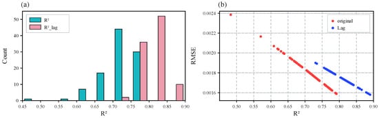
Figure 8 compares the 100 repeated fits for each input scheme described in Section 2.6. The results show that the model trained with the raw data has an average R² value of 0.719, while the model trained with the time-lagged data has an average R² value of 0.809. The model trained with the time-lagged data has a higher reported mean R² and a visually narrower R² distribution, with R² values more concentrated between 0.75 and 0.85. Additionally, RMSE is negatively correlated with R², where higher R² corresponds to lower RMSE, as expected for residual-based R² and RMSE evaluated on a common target series.

Figure 8. The R² distribution of 100 LSTM models randomly trained on the raw data and time-lagged data from Wuli Lake (a) and the corresponding scatter plot of RMSE and R² (b).

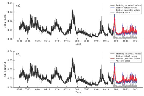
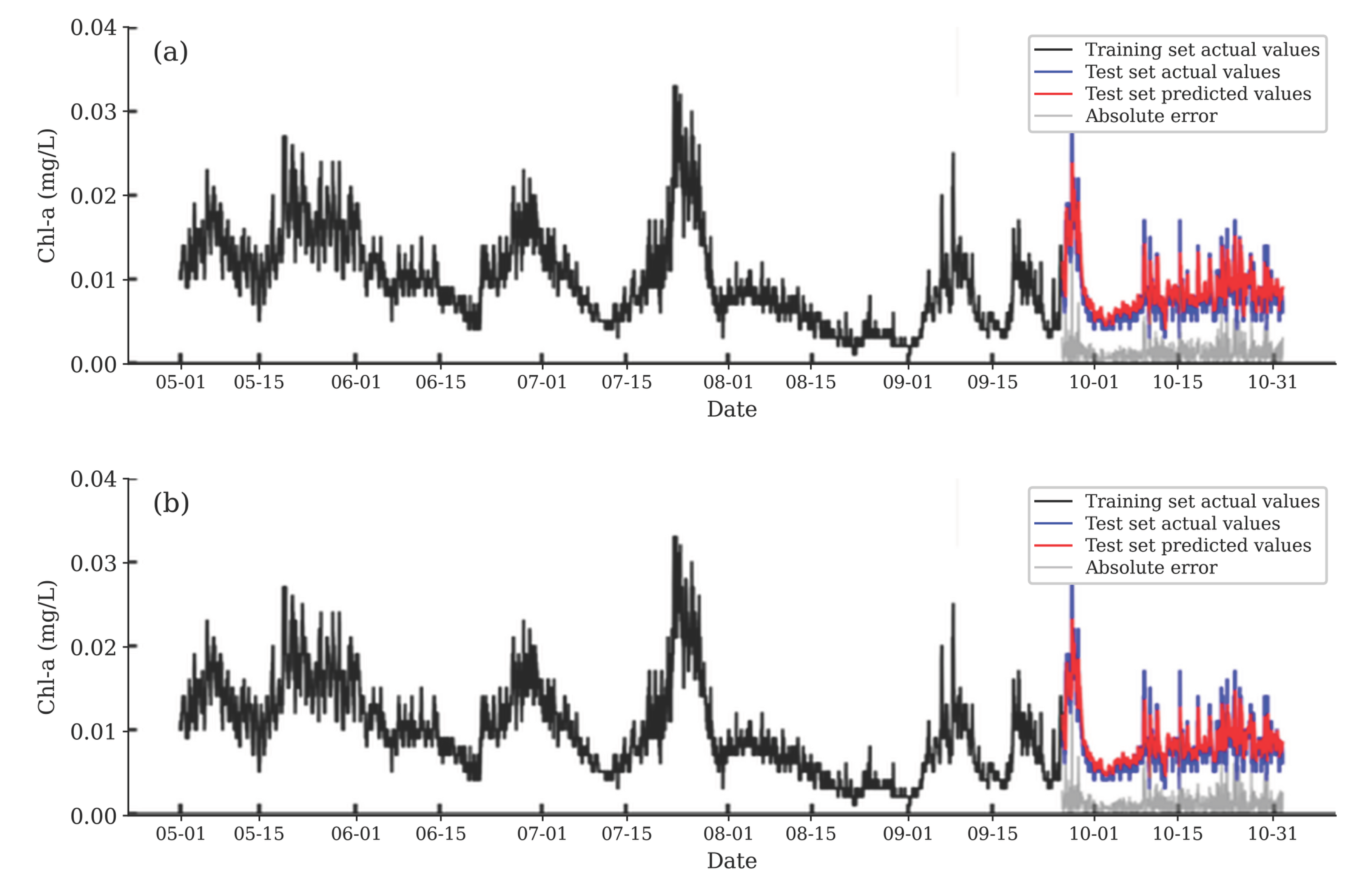
The Chl-a concentration prediction results of the LSTM model trained on raw data and time-lagged data for the Wuli Lake watershed (as shown in Figure 9) indicate that the model effectively captures the variation trends of Chl-a concentration, particularly at the extreme point around September 25. However, in certain periods, especially in mid-to-late October, the prediction accuracy of the model trained on time-lagged data appears better than that of the raw data model. This improvement may be attributed to the ability of time-lagged data to better reflect the lag effects of meteorological factors such as temperature and wind speed when the LSTM model learns patterns from historical data through a sliding window, thereby enhancing the model’s sensitivity to these relationships and improving prediction accuracy.

Figure 9. Time-series predictions of Chl-a concentration in the Wuli Lake watershed based on the LSTM model using raw data (a) and time-lagged data (b).

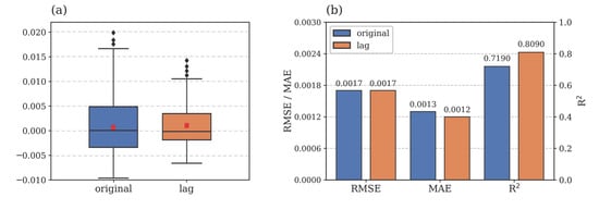
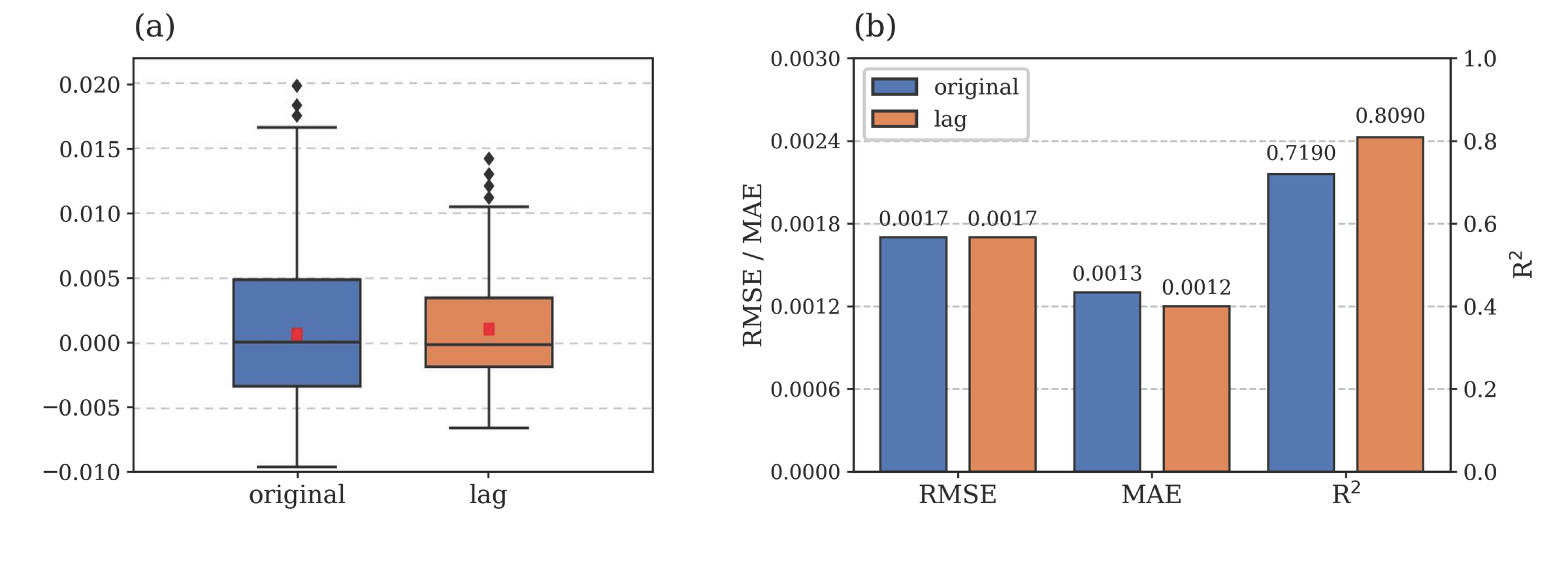
As shown in Figure 10a, the lag-aware model has a visually narrower interquartile range of prediction bias. Figure 10b shows that mean R² increased from 0.719 to 0.809 (an absolute increase of 0.090, or approximately 12.5% relative to the original value), while MAE decreased from 0.0013 to 0.0012 mg/L. Both RMSE values round to 0.0017 mg/L at the displayed precision; therefore, the figure supports improved explained variance, MAE, and bias dispersion but does not support a claim of a material RMSE reduction without additional decimal places or a statistical test. The reported MAE change is approximately 0.1 µg/L (1.3 to 1.2 µg/L); both reported RMSE values equal 1.7 µg/L after rounding.

Figure 10. Prediction performance of LSTM models using original and lag-aligned inputs: (a) box plots of prediction bias, where the center line indicates the median, the box spans the 25th–75th percentiles, and whiskers and points show the plotted spread and outliers; (b) comparison of RMSE, MAE, and R².

In summary, aligning meteorological inputs with the identified lag window improved the LSTM model’s explained variance and reduced typical absolute error and prediction-bias dispersion. The reported mean metrics favored the lag-aligned model, while RMSE remained essentially unchanged at the precision shown. Viewed as a removal control, the unshifted-input model evaluates the combined lag-alignment step. The observed difference cannot be assigned separately to temperature or wind, and it does not demonstrate superiority over other model families.

3.7. Factorial Ablation of Temperature and Wind Alignment

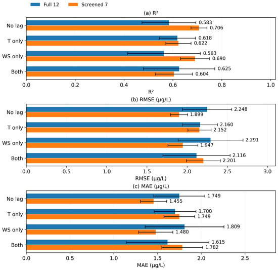
Figure 11 compares the four lag configurations under full and screened inputs on the same 743 test targets. With all 12 inputs, joint alignment has mean R² 0.625, RMSE 2.116 µg/L and MAE 1.615 µg/L, compared with 0.583, 2.248 µg/L and 1.749 µg/L without alignment. This within-design direction agrees with the full-input comparison in Section 3.6. All four configurations retain temperature and wind as predictors; only their offsets differ.

Figure 11. LSTM performance under lag ablation. (a) R²; (b) RMSE; (c) MAE. Blue: full inputs; orange: screened inputs. Bars show mean ± SD across five paired fits on 743 common test targets. T only and WS only apply one lag.

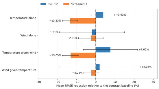
Figure 12 shows the separate and conditional lag contributions. In the full-input models, temperature-only alignment reduces mean RMSE by 3.93%, whereas wind-only alignment increases it by 1.91%. Temperature added to a wind-aligned model reduces mean RMSE by 7.65%, and wind added after temperature reduces it by 2.04%. Separate and conditional contrasts therefore differ: a near-zero standalone wind benefit is compatible with a positive joint contrast. This is a predictive interaction within the chosen input set, not evidence of independently significant ecological effects.

Figure 12. Temperature and wind lag contributions. Blue: full inputs; orange: screened inputs. Bars show relative RMSE reduction ± paired SD, normalized by the baseline mean RMSE. Positive values indicate improvement; conditional contrasts add one lag given the other.

After redundancy removal, the unshifted seven-input model has mean R² 0.706 and RMSE 1.899 µg/L; joint alignment has R² 0.604 and RMSE 2.201 µg/L. Thus, screening changes both baseline performance and the response to alignment. The full-input alignment advantage does not persist under this reduced configuration. This result indicates that the predictive benefit of lag alignment depends on the input-variable set and should not be generalized across predictor configurations. The persistence reference achieves R² of 0.767 and RMSE of 1.692 µg/L, outperforming the mean performance of the LSTM configurations evaluated in the ablation experiments. Independent-year validation and additional temporal splits are needed before an operational advantage can be claimed.

4. Discussion

The rank analysis and lag analysis describe different aspects of the lake response. TP, turbidity and TN have the strongest concurrent associations, but pH–DO, WT–EC and TP–turbidity correlations demonstrate substantial overlap among candidate indicators. The retained-driver partial coefficients show how marginal association rankings can change when other variables are controlled. This is consistent with Qu et al. [7], who combined rank screening and prior knowledge before interpreting Taihu drivers, and with the collinearity concerns reviewed by Dormann et al. [8]. Unlike a spatial or ecological-state driver ranking, the present analysis concerns one season at a fixed location. Negative nutrient associations may reflect consumption and shared temporal structure, while algal density and Chl-a both describe biomass. We therefore interpret ranks as evidence of association and redundancy, not as a causal ranking of growth controls.

The hydrological context helps explain why meteorological lags are detectable in Wuli Lake. The lake is shallow and relatively enclosed, with an estimated volume of 1.02 × 10⁷ m³ and an idealized exchange period of approximately 2.4 d under the representative 50 m³/s diversion scenario. Published hydrodynamic modeling indicates that circulation nevertheless remains spatially heterogeneous and depends strongly on wind, diversion discharge, and outlet configuration [21]. Wind can resuspend sediment in shallow Lake Taihu systems [6], increasing turbidity and redistributing nutrients, but it can also disperse surface accumulations and reduce light exposure. The high Chl-a–wind cross-correlation (maximum 0.90) therefore indicates strong short-term coupling, not a uniformly positive biological effect of wind. Importantly, the 6–9 h lag identified here is much shorter than the idealized whole-lake exchange period; it is more plausibly associated with local mixing, cell redistribution, air–water heat transfer, and physiological adjustment near OBV than with complete renewal of the lake volume.

The magnitude of a Chl-a lag is expected to vary with ecosystem type and temporal resolution. Zhang et al. [10] showed that chlorophyll response lags change with water-column stability and nutrient background in a deep reservoir, while Liu et al. [11] reported an approximately 10 d antecedent response in a hydrologically regulated river using 10 d observations. These longer lags do not conflict with the present sub-daily result; instead, they show that the resolved lag depends on hydrodynamic scale, biological state, driver, and sampling interval. The physiological basis for delayed microalgal growth has also long been recognized [11]. In this study, cross-wavelet phase estimates (7.48 h for air temperature and 6.44 h for wind speed) and cross-correlation maxima (9 h and 8 h, respectively) are close but not identical because the methods summarize phase and correlation differently. These central estimates suggest a sub-daily association for this station and season, with appreciable variation, rather than a bounded 6–9 h interval or universal fixed lags of exactly 7.48 h and 6.44 h.

The full-input prediction comparison shows increased mean R² from 0.719 to 0.809, reduced MAE from 0.0013 to 0.0012 mg/L and narrower bias dispersion, with both RMSE values approximately 0.0017 mg/L at the displayed precision. The factorial analysis then assigns alignment effects separately within the full-input architecture and tests them after redundancy removal. In the factorial ablation experiments, joint lag alignment improves mean prediction performance with the full input set, whereas the contribution of each individual lag depends on whether the other lag is included. This advantage does not persist with the screened input set. Redundant environmental variables may carry different temporal information even when their concurrent associations overlap. Removing them changes what the network must learn from temperature and wind history; a low-VIF set is therefore more interpretable without necessarily preserving the same lag response in prediction. We cannot attribute these changes to a unique physiological pathway or claim that the wavelet offsets are universally optimal.

This interpretation complements rather than duplicates existing hybrid forecasts. Liu et al. [14] demonstrate multi-resolution benefits from wavelet-enhanced forecasting, while hydrodynamic–LSTM coupling [15] incorporates transport information explicitly. Our factorial contrasts focus on the incremental effect of specific input offsets and show its dependence on covariate choice. Fournier et al. [16] also evaluate forecast skill relative to a displaced signal, which matters for high-frequency records with strong persistence. The persistence performance here shows why an improvement between two LSTM configurations alone is insufficient to establish useful forecast skill. Together, the full-input and screened-input results show that the predictive value of lag alignment depends on predictor selection, which should be considered when configuring models for operational use.

For cyanobacterial-bloom management, the result is most useful as a design rule for a tiered early-warning workflow rather than as a stand-alone alarm threshold. A prospective system could update hourly, ingest the antecedent meteorological and water-quality observations required by the model, and issue a Chl-a forecast with separately validated uncertainty estimates. Depending on location and risk, responses may include targeted mixing or aeration, optimized water diversion, interception or collection of surface accumulations, and intensified monitoring of drinking-water or recreational zones [2]. The lag relationship itself does not automatically provide a validated 6–9 h warning lead: that lead time must be tested by defining a future target (for example, Chl-a at t + 6 h) and evaluating threshold-specific sensitivity, false-alarm rate, and usable lead time. This distinction links the statistical improvement to an operational decision without overstating current model capability.

5. Conclusions

Using hourly observations from one fixed station in Wuli Lake between 1 May and 31 October 2023, this study identified sub-daily Chl-a lag associations with meteorological forcing. Cross-wavelet phase analysis estimated lags of 7.48 h for air temperature and 6.44 h for wind speed, while wavelet cross-correlation peaked at 9 h and 8 h, respectively; together, these central estimates suggest station- and season-specific sub-daily timing, with variability rather than two universal fixed values.

For the full 12-input model, incorporating lag-aligned meteorological inputs into the LSTM model increased mean R² from 0.719 to 0.809 (ΔR² = 0.090; approximately 12.5%), reduced MAE from 0.0013 to 0.0012 mg/L, and narrowed prediction-bias dispersion across repeated runs. RMSE remained approximately 0.0017 mg/L at the precision shown. The central conclusion is therefore that wavelet-derived temporal alignment increased reported explained variance and reduced typical absolute error for this hourly one-site dataset.

Factorial ablations quantified temperature and wind alignment separately. The factorial ablation experiments showed that joint temperature and wind-speed lag alignment improved mean prediction performance with the full input set, but this benefit did not persist with the screened input set. The timing information therefore has configuration-dependent predictive value; neither a strong wavelet association nor a low-VIF input set guarantees an alignment gain.

The result provides a practical basis for designing rolling Chl-a forecasts that use antecedent meteorological information and for testing management-relevant bloom-warning lead times. It does not, by itself, establish causality, a universal lag, or a validated operational warning threshold.

Transfer to routine cyanobacterial-bloom management requires multi-season and multi-site observations, measured hydrological exchange, rolling-origin or independent-year validation, uncertainty quantification, and event-based metrics such as sensitivity, false-alarm rate, and usable lead time.

References

- Huo, D.; Gan, N.; Geng, R.; Cao, Q.; Song, L.; Yu, G.; Li, R. Cyanobacterial blooms in China: Diversity, distribution, and cyanotoxins. Harmful Algae 2021, 109, 102106. [Google Scholar] [CrossRef] [Scilit]
- Song, L.; Jia, Y.; Qin, B.; Li, R.; Carmichael, W.W.; Gan, N.; Xu, H.; Shan, K.; Sukenik, A. Harmful cyanobacterial blooms: Biological traits, mechanisms, risks, and control strategies. Annu. Rev. Environ. Resour. 2023, 48, 123–147. [Google Scholar] [CrossRef] [Scilit]
- Xiao, X.; Peng, Y.; Zhang, W.; Yang, X.; Zhang, Z.; Ren, B.; Zhu, G.; Zhou, S. Current status and prospects of algal bloom early warning technologies: A Review. J. Environ. Manag. 2024, 349, 119510. [Google Scholar] [CrossRef] [Scilit]
- Reinl, K.L.; Brookes, J.D.; Carey, C.C.; Harris, T.D.; Ibelings, B.W.; Morales-Williams, A.M.; Domis, L.N.D.S.; Atkins, K.S.; Isles, P.D.F.; Mesman, J.P.; et al. Cyanobacterial blooms in oligotrophic lakes: Shifting the high-nutrient paradigm. Freshw. Biol. 2021, 66, 1846–1859. [Google Scholar] [CrossRef] [Scilit]
- Frau, D. Towards a quantitative definition of Cyanobacteria blooms. Environ. Rev. 2023, 31, 643–651. [Google Scholar] [CrossRef] [Scilit]
- Wang, J.; Yuan, Y.; Yu, Z.-G.; Qu, S.; Li, W. Effect of turbulence driven by wind on sediment suspension under different submerged vegetation density in Lake Taihu. Ecol. Indic. 2023, 154, 110767. [Google Scholar] [CrossRef] [Scilit]
- Qu, S.; Wang, J.; Kumar, A.; Yu, Z.; Zhao, W. Identification of driving factors for chlorophyll-a in multi-stable shallow lakes of China employing machine learning methods. Ecohydrology 2023, 16, e2590. [Google Scholar] [CrossRef] [Scilit]
- Dormann, C.F.; Elith, J.; Bacher, S.; Buchmann, C.; Carl, G.; Carré, G.; Marquéz, J.R.G.; Gruber, B.; Lafourcade, B.; Leitão, P.J.; et al. Collinearity: A review of methods to deal with it and a simulation study evaluating their performance. Ecography 2013, 36, 27–46. [Google Scholar] [CrossRef] [Scilit]
- Lofton, M.E.; Brentrup, J.A.; Beck, W.S.; Zwart, J.A.; Bhattacharya, R.; Brighenti, L.S.; Burnet, S.H.; McCullough, I.M.; Steele, B.G.; Carey, C.C.; et al. Using near-term forecasts and uncertainty partitioning to inform prediction of oligotrophic lake cyanobacterial density. Ecol. Appl. 2022, 32, e2590. [Google Scholar] [CrossRef] [Scilit]
- Zhang, M.; Niu, Z.; Cai, Q.; Xu, Y.; Qu, X. Effect of water column stability on surface chlorophyll and time lags under different nutrient backgrounds in a deep reservoir. Water 2019, 11, 1504. [Google Scholar] [CrossRef] [Scilit]
- Liu, C.; Chen, Y.; Zou, L.; Cheng, B.; Huang, T. Time-lag effect: River algal blooms on multiple driving factors. Front. Earth Sci. 2022, 9, 813287. [Google Scholar] [CrossRef] [Scilit]
- Torrence, C.; Compo, G.P. A practical guide to wavelet analysis. Bull. Am. Meteorol. Soc. 1998, 79, 61–78. [Google Scholar] [CrossRef] [Scilit]
- Grinsted, A.; Moore, J.C.; Jevrejeva, S. Application of the cross wavelet transform and wavelet coherence to geophysical time series. Nonlinear Process. Geophys. 2004, 11, 561–566. [Google Scholar] [CrossRef] [Scilit]
- Liu, M.; He, J.; Huang, Y.; Tang, T.; Hu, J.; Xiao, X. Algal bloom forecasting with time-frequency analysis: A hybrid deep learning approach. Water Res. 2022, 219, 118591. [Google Scholar] [CrossRef] [Scilit]
- Zheng, L.; Wang, H.; Liu, C.; Zhang, S.; Ding, A.; Xie, E.; Li, J.; Wang, S. Prediction of harmful algal blooms in large water bodies using the combined EFDC and LSTM models. J. Environ. Manag. 2021, 295, 113060. [Google Scholar] [CrossRef] [Scilit]
- Fournier, C.; Fernandez-Fernandez, R.; Cirés, S.; López-Orozco, J.A.; Besada-Portas, E.; Quesada, A. LSTM networks provide efficient cyanobacterial blooms forecasting even with incomplete spatio-temporal data. Water Res. 2024, 267, 122553. [Google Scholar] [CrossRef] [Scilit]
- Mozo, A.; Morón-López, J.; Vakaruk, S.; Pompa-Pernía, Á.G.; González-Prieto, Á.; Pascual Aguilar, J.A.; Gómez-Canaval, S.; Ortiz, J.M. Chlorophyll soft-sensor based on machine learning models for algal bloom predictions. Sci. Rep. 2022, 12, 13529. [Google Scholar] [CrossRef] [Scilit]
- Sun, G.; Zhu, W.; Qian, X.; Wei, C.; Xie, P.; Shi, Y.; Cao, X.; He, Y. Machine learning models for chlorophyll-a forecasting in a freshwater lake: Case study of Lake Taihu. Water 2025, 17, 1219. [Google Scholar] [CrossRef] [Scilit]
- Heggerud, C.M.; Xu, J.; Wang, H.; Lewis, M.A.; Zurawell, R.W.; Loewen, C.J.G.; Vinebrooke, R.D.; Ramazi, P. Predicting imminent cyanobacterial blooms in lakes using incomplete timely data. Water Resour. Res. 2024, 60, e2023WR035540. [Google Scholar] [CrossRef] [Scilit]
- Chen, K.; Bao, X.; Shi, L.; Chen, W.; Lan, C.; Xu, H.; Hu, H. Ecological restoration engineering in Lake Wuli, Lake Taihu: A large enclosure experiment. J. Lake Sci. 2006, 18, 139–149. [Google Scholar] [CrossRef] [Scilit]
- Mi, C.; Mao, J.; Dai, H.; Dai, L. Influence of different water diversion schemes on hydrodynamic characteristics of Wulihu Lake. China Rural Water Hydropower 2013, 5, 53–56. (In Chinese) [Google Scholar]
- Yu, H.; Hutson, A.D. A robust Spearman correlation coefficient permutation test. Commun. Stat. Theory Methods 2024, 53, 2141–2153. [Google Scholar] [CrossRef] [Scilit]
Disclaimer/Publisher’s Note: The statements, opinions and data contained in all publications are solely those of the individual author(s) and contributor(s) and not of MDPI and/or the editor(s). MDPI and/or the editor(s) disclaim responsibility for any injury to people or property resulting from any ideas, methods, instructions or products referred to in the content. |
© 2026 by the authors. Licensee MDPI, Basel, Switzerland. This article is an open access article distributed under the terms and conditions of the Creative Commons Attribution (CC BY) license.