An Innovative Morphometric Model—The Soil Loss Model Utilizing Watershed Hierarchy and the RUSLE Framework: The Buzău River Basin, Romania

Abstract

Soil loss due to erosion is a form of land degradation, having significant effects on agricultural productivity, water resource quality, and food security. The morphometric analysis of the drainage network is based on mathematical relationships and geometric progressions. In previous studies, several morphometric parameters have been analyzed in relation to stream order. While numerous studies have assessed soil loss at the watershed level, its spatial variability at the sub-watershed level remains less understood, even though it can highlight sectors that disproportionately contribute to soil loss. Thus, this study aims to analyze whether the RUSLE-estimated soil loss values follow the same morphometric relationship and geometric progressions by examining the hierarchical distribution of soil loss in the 39 sub-watersheds of the Buzău River Basin. The methodology consisted of extracting the mean and summed values of soil loss from the RUSLE2015 raster for all 9369 sub-watersheds, which were hierarchized into seven orders of streams. We created two laws of summed and mean soil loss, and the law of the number of sub-watersheds corresponds to the law of the number of segments. The three data series exhibit geometric progression patterns for which ratios have been calculated. Internal variations in the estimated soil loss have been observed. The sub-Carpathian sector is the most susceptible to the estimated mean (66%) and total (73%) soil loss. Sub-watersheds whose area is smaller or comparable with that of other sub-watersheds in the Carpathian sector exhibited much higher soil loss values (SW 11- 0.16 t ha⁻¹ yr⁻¹ vs. SW 33- 3.36 t ha⁻¹ yr⁻¹). The Slănic sub-Watershed loses a total of 202,325.48 t yr⁻¹, while Bâsca loses only 50,573.86 t yr⁻¹, even though its area is much larger (78,300 ha). The highest values of mean soil loss are recorded in Oleșești, at 9.19 t ha⁻¹ yr⁻¹. These results can support authorities in identifying and prioritizing sub-watersheds that may require soil conservation measures and can be reproduced in watersheds with different characteristics.

1. Introduction

Hydrographic basins are regarded as the basic geomorphological units of lands (Gâștescu et al., 2006; Posea, 2005) [1,2], in which an attempt is made to achieve a balance of this open system, represented by the constant exchange of matter and energy (Zăvoianu, 1978) [3]. Morphometry is a sub-field of geomorphology concerned with quantifying linear, areal, and volume dimensions (Clarke, 1966) [4]. Its use has allowed for the detailed evaluation of the morphodynamics of watersheds (Zăvoianu et al., 2013) [5], as well as their response to fluctuations in the river’s general base level (Demoulin, 2011) [6].

The number of segments, their total length, the average slope of the watershed and the first-order valley, and the area or altitudes are the subject of specific morphometric laws (Horton, 1932; Horton, 1945; Strahler, 1952) [7,8,9]. These constitute successively increasing data series that can be graphically depicted in a semilogarithmic coordinate system, forming morphometric models of drainage, slopes, and areas (Zăvoianu, 1978; Armaș, 1999; Marinescu, 2007; Codreanu, 2017) [3,10,11,12]. Through these morphometric models, spatial differences between sub-watersheds can be analyzed, as they allow for the evaluation of the degree of development and organization of the hydrographic network, as well as the stage of evolution or equilibrium reached by the respective watershed (Zăvoianu, 1978) [3]. Zăvoianu (2011, 1988) [13,14] applied a series of morphometric models to the watersheds Buzău, Ialomița, and Bârlad. Cruceru (2011) [15] and Cruceru and Herișanu (2011) [16] conducted a comprehensive analysis of the Sărățel Watershed, particularly focusing on the hydrographic network; Grecu (1992) [17] examined the Hârtibaciu Watershed; Minea (2012; 2013) [18,19] researched the Bâsca River Watershed, and Minea, I.S. (2011) [20] studied the rivers within the Buzău Watershed.

Recent studies in Romania use GIS models and satellite images to quantify soil losses, demonstrating that controlled pasture management and reforestation of slopes can reduce soil losses in the sub-Carpathians (Vîrghileanu et al., 2024) [21]. More recently, Vîrghileanu et al. (2026) [22] compare four methods for estimating the C factor (cover-management factor), using Sentinel-2 images. The Revised Universal Soil Loss Equation (RUSLE) was applied in the Bâsca Chiojdului Watershed to analyze the influence of LS (slope length and steepness factor) and C factors in identifying sectors affected by erosion (Rizac et al., 2025) [23]. In the context of climate change, the highest soil erosion values will be recorded in hilly and plateau regions (Patriche, 2023) [24], areas where erosion is the determining process of agricultural land degradation (Prăvălie et al., 2025) [25]. The RUSLE model has been applied in numerous studies related to watershed management and has been validated through direct measurements of the sediment volume accumulated in the Eșalnița Watershed (Nistor et al., 2025) [26].

Soil loss is recognized as a major problem affecting food security due to the loss of crops (Alewell et al., 2019; Tilman et al., 2011) [27,28]. Each year, 12 million hectares of fertile soil are lost due to erosion within the European Union (Panagos et al., 2022) [29], and its natural restoration is a prolonged process (FAO, 2015) [30]. The amount of soil that detaches from slopes is transported by water and redistributed by the river network within the watershed (Andualem et al., 2023) [31]. This process results in the destabilization of slopes and riverbeds (Zhao et al., 2022) [32], as well as reservoir clogging (Senapati & Das, 2019) [33]. Between soil erosion and physical-geographical conditions, there are interdependent relationships (Panagos et al., 2022) [29]. The annual soil loss of approximately 5.2 million hectares of forest vegetation contributes significantly to the expansion of degraded land worldwide (Prăvălie et al., 2021; Borrelli et al., 2017) [34,35]. To enhance sustainable resource management and biodiversity conservation (Piacentini et al., 2018) [36], the Universal Soil Loss Equation (USLE) was established by Wischmeier and Smith (1978) [37], which was subsequently revised into the Revised Universal Soil Loss Equation (RUSLE) (Renard et al., 1997) [38]. This model was applied in numerous studies (Choudhury et al., 2022; Borrelli et al., 2016; Panagos et al., 2015) [39,40,41].

The RUSLE model and machine learning techniques can estimate soil loss at the watershed scale, but their performance in capturing spatial variation and hierarchical distribution along the drainage network has received limited attention. Morphometric parameters directly affect flow velocity, the soil loss intensity, and sediment transport and vary locally. Consequently, recent studies may either underestimate or overestimate soil loss (Pastor et al., 2024) [42].

Previous research studies have analyzed the distribution of various morphometric parameters (lengths, slopes, perimeters, surfaces) in relation to the successive orders of the drainage network in the Horton–Strahler system. Different morphometric models of basin areas, basin perimeters, mean altitudes, mean stream slopes, and even a model of mean discharges for the Ialomița watershed have been developed (Zăvoianu, 1978, 1985) [3,43]. Therefore, morphometric laws can also be extended to other parameters.

This study aims to demonstrate that the RUSLE-estimated soil loss also obeys the same morphometric relationship. This study analyzes the 39 sub-watersheds in the Buzău River Basin. The main objectives are:

(a)

The delimitation and hierarchization of the hydrographic network in the Horton–Strahler system;

(b)

The quantification and cartographic representation of RUSLE-estimated soil loss;

(c)

The identification of the most susceptible sub-watersheds to soil loss;

(d)

The application of the morphometric model of soil loss based on the methodology proposed by Horton (1945) [8], further complemented by Zăvoianu (1978) [3] to highlight the hierarchical spatial variability of RUSLE2015-estimated soil loss;

(e)

The formulation and application of morphometric relationships regarding mean and summed soil loss;

(f)

Interpretation of morphometric relationships and soil loss distribution within the hierarchy of sub-watersheds.

2. Study Area

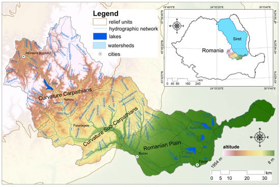
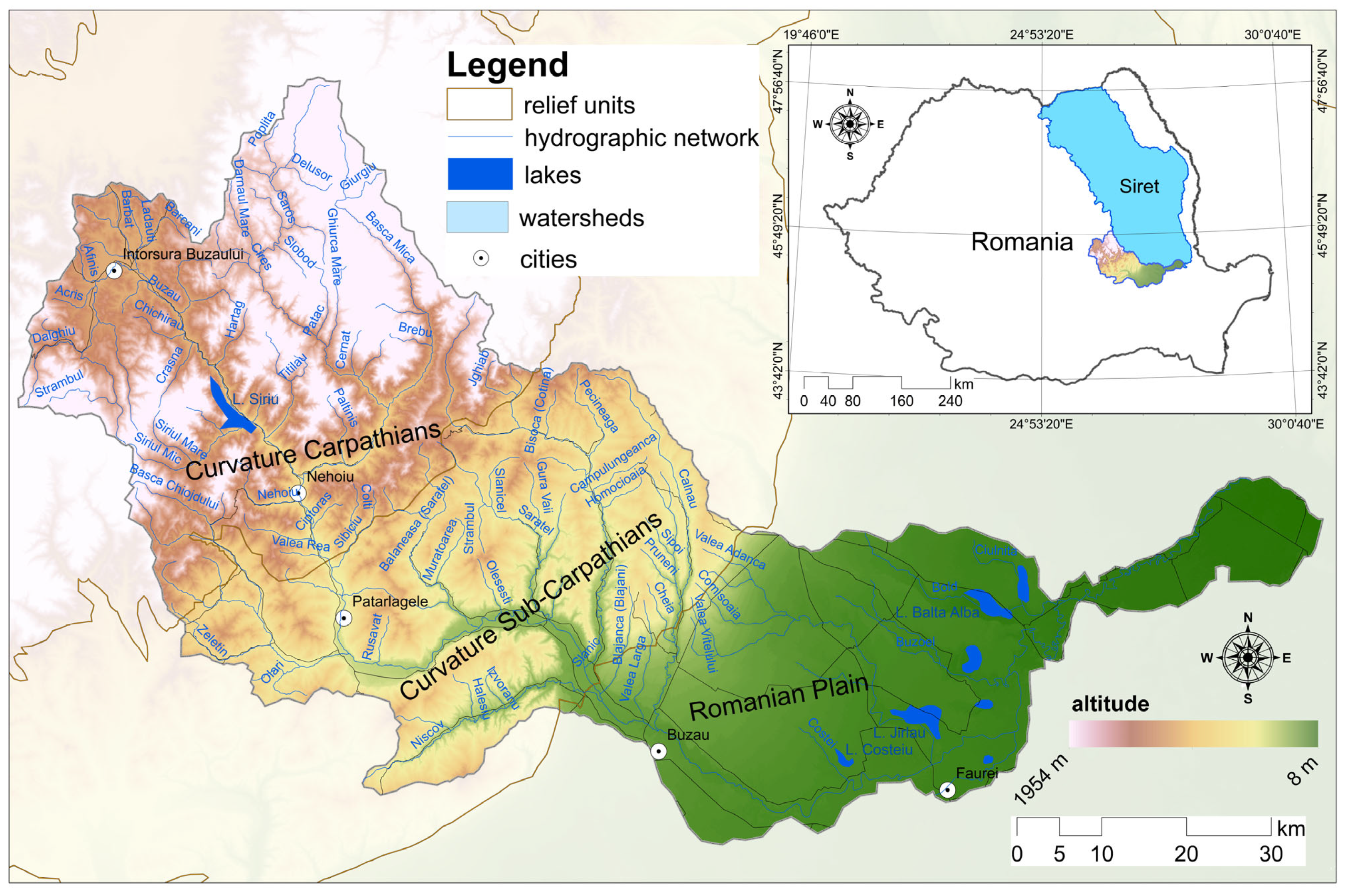
The Buzău Watershed covers a total area of 5264 km² (Cadastral Atlas—1992) [44] and represents 12.9% of the Siret watershed area (Minea, 2011) [20], located in the southern and southwestern regions of the basin. It accounts for 2.2% of Romania’s total area (Figure 1). The watershed is divided into three distinct relief subunits: the upper sector, which comprises 48% of the Curvature Carpathians; the middle sector, situated within the Curvature sub-Carpathians (46%), which is particularly prone to landslides and hydraulic erosion processes (Micu, 2010) [45]; and the lower sector, positioned in the low area of the Romanian Plain (6%). The Buzău River originates at an elevation of 1242 m in the Ciucaş Massif and discharges into the Siret River at an altitude of 8 m, totaling a length of 302 km.

Figure 1. The geographical location of the Buzău Watershed in Romania.

The analyzed area shows great lithological diversity, from resistant rocks (Tarcău sandstone facies, Ciucaș limestones and conglomerates) to molasse deposits (Eocene clays, Burdigalian marls, Badenian tuffs) and fine loess deposits (Minea, 2012) [18]. In the plain sector, the largest distribution is held by quaternary loess deposits (58%). In the sub-Carpathian sector, 33% of the area is covered by Pliocene formations of sands, marls, and clays, found at the level of the external ridge (Culmea Budei, Blăjanilor, and Bisocăi). These are complemented by salt deposits in the Slănic sub-Watershed, in the communes of Mânzălești and Lopătari. In this sector, in the Pâclele Murătoarea sub-Watershed, muddy flows occur on the clayey substrate, leading to the development of rills, gullies, and the mud volcanoes of Pâclele Mari and Pâclele Mici. The largest area in the Carpathian sector is occupied by the Tarcău sandstone facies (33%), found in the Bâsca, Harțag, Ghiurca Mare, and Cășoaca Mare sub-watersheds. The Buzău Watershed has a temperate-continental climate, with rainfall controlled by altitude and the orographic effect. Mean annual precipitation varies from approximately 500–550 mm in the plain sector to 900–1000 mm in the Ciucaș and Penteleu peaks. Consequently, there is a greater potential for erosion in the upper sectors of the watershed than in the plain area, particularly during intense summer rainfall events and prolonged spring precipitation combined with snowmelt.

Cambisols predominate in the Buzău Watershed, covering 37% of the area. The Carpathian sector accounts for approximately 71% of the area. Forest vegetation covers an area of 2232 km² (42%) in the Buzău Watershed. The Bâsca sub-Watershed has a share of 79% of the forest cover. Mixed forests cover Zăbrătău, Harțag, and Cășoaca Mare at percentages exceeding 64%. These occur locally in the Strâmbul sub-Watershed (7.57 km²) and in the upper part of the Bâsca Chiojdului, Nehoiu, and Siriul Mare sub-watersheds. Deciduous forests are found in the watersheds: Nișcov (79.33%), Sibiciu (92%), Bâsca Chiojdului (60.03%), and Pănătău (78.17%).

3. Materials and Methods

The present study was conducted using the ArcGIS 10.6.1 program to create the database and spatialization of the morphometric characteristics. The delimitation of the sub-watersheds involved the use of the dataset provided by the National Administration “Apele Române” [46], which was revised based on the 1:25,000 topographic map, leading to the identification of 39 sub-watersheds. The 39 analyzed sub-watersheds have distinct and independent drainage networks, selected based on criteria such as the main course being longer than 5 km, being a direct tributary of the Buzău River, having a permanent flow, and the watershed area being larger than 10 km². Their selection corresponds to the official inventory (Cadastral Atlas—1992) [43] and aims to standardize the units of analysis, so that the comparison of morphometric parameters and the hierarchical analysis of the drainage network can be carried out. The sub-watersheds have been classified into one of the three sectors. The method employed to assign the sub-watersheds located at the contact between two geographic subunits aims to assess the degree of development of the drainage network. The hydrographic network was generated automatically using the Hydrology function from the ArcToolbox menu and hierarchized according to Horton (1945) [8] and standardized by Strahler (1952) [9]. The 39 selected sub-watersheds correspond to the highest-order drainage unit in their respective drainage system and may contain several lower-order sub-watersheds. The hierarchical order of each sub-watershed (µ) was established based on the hierarchy of the drainage network and the order of its main watercourse. Thus, first-order (N₁) sub-watersheds correspond to streams located at the highest altitudes within the hydrographic network, being drained by a single watercourse. The order of magnitude increases progressively along the drainage network with the confluence of two streams that hold the same order. The confluence of two first-order streams leads to the immediate attainment of the next order of magnitude, N₂. All second-order courses correspond to second-order sub-watersheds, the same principle being applied to the most distant segments. N_s represents the course that holds the highest order in the watershed, which is seven, respectively. It should be noted that neither the area nor the affiliation of the sub-watersheds to a certain relief unit was a criterion considered. Sub-watersheds of the same order can vary in size, and a more developed hydrographic network will result in a larger sub-watershed order. We have classified the sub-watersheds located at the boundary between two relief units based on the proportion of river segments, so that if over 50% of the segments are classified in the sub-Carpathian sector, then the respective sub-watershed is classified in this sector and not in the Carpathian one.

We used the existing raster (water erosion—RUSLE2015), available through the European Soil Data Centre (ESDAC) [47]. This model estimates soil loss associated with sheet erosion and rill erosion. With a spatial resolution of 100 m × 100 m, each pixel in this raster represents the mean annual soil loss, quantified in t ha⁻¹ yr⁻¹ (Borrelli et al., 2017; Panagos et al., 2015) [35,41]. Although the dataset is called RUSLE2015, it uses the year 2010 as the reference year. The RUSLE2015 dataset has been used at the European level in comparison with national data available in EIONET-SOI (Panagos et al., 2015) [41]. Subsequently, it has been used in numerous studies evaluating and comparing estimated soil loss with measured erosion rates (Patriche, 2023; Napoli et al., 2016) [24,48], demonstrating its validity.

Since the raster is in the ETRS89 Lambert Azimuthal Equal Area map projection, it needed to be transformed into the Stereo 70 projection system to intersect with the basin boundary using the Projections and Transformations—Project Raster function. The resampling method used was Nearest, and the output cell size remained 100 × 100 m. Through Spatial Analyst Tools—Extraction—Extract by Mask, we clipped each raster according to the boundary of all sub-watersheds of different orders. The RUSLE model integrates five parameters: the rainfall erosion factor (R), the soil erodibility factor (K), the slope length and steepness factor (LS), the cover management factor (C), and the support practice factor (P). Therefore, it is important to specify that the values obtained from RUSLE2015 do not constitute direct measurements of the actual soil loss from a specific year but rather a spatial estimate based on this equation.

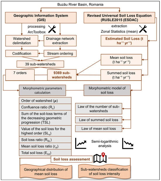
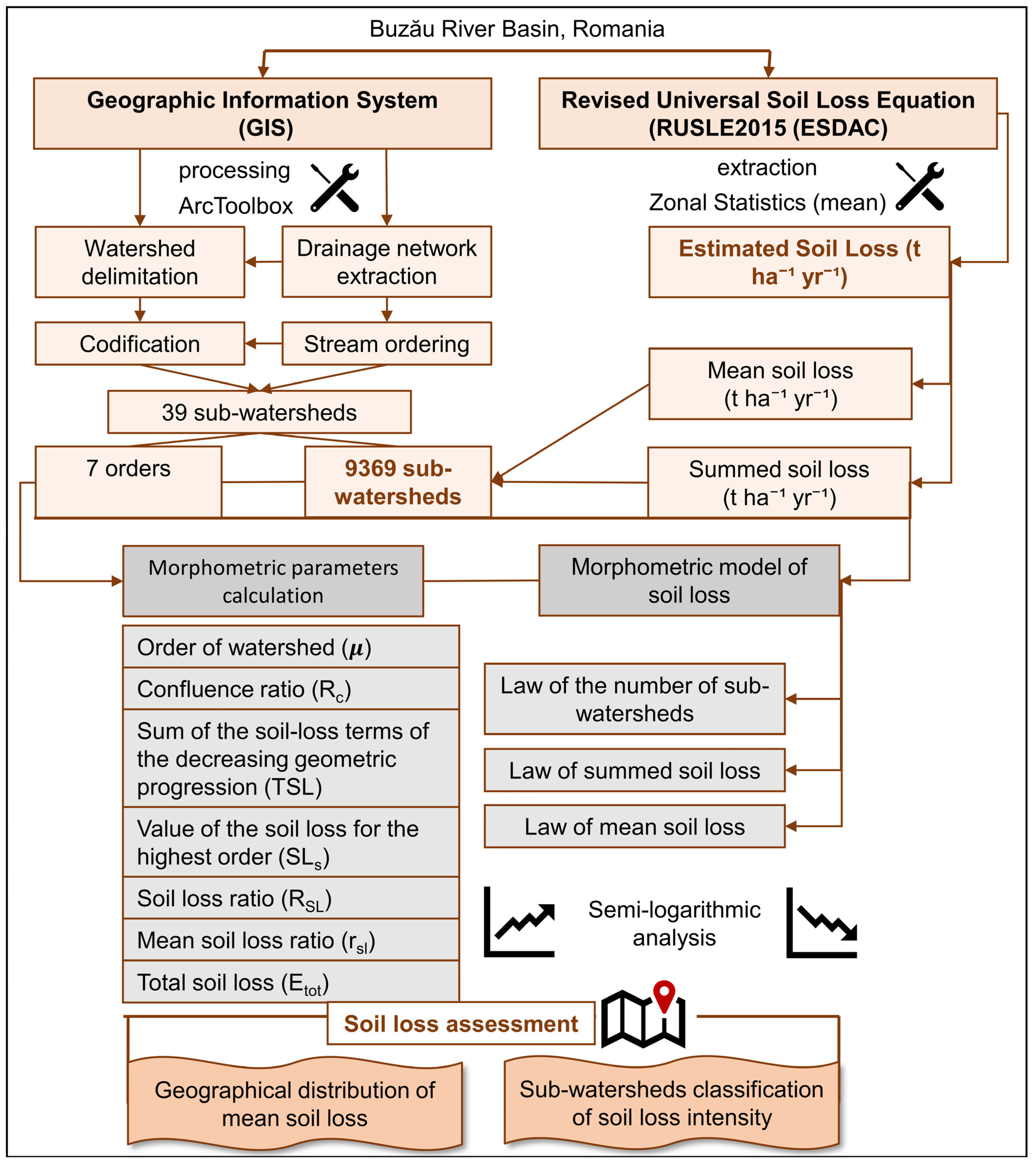
The methodological flow is illustrated in Figure 2. From the Attribute Table menu of the polygons, we extracted the areas (S) and the number of sub-watersheds of different orders (µ). The extraction of mean and summed soil loss values was carried out using the clipped rasters. A main limitation when using rasters is the precise extraction of mean and summed values over distinct spatial units. In a given area, multiple pixels with their own values overlap. For example, within the raster of first-order sub-watersheds in the Bâsca sub-Watershed, the sum is 12,891.90 t ha⁻¹ yr⁻¹, as it represents the sum of the 33,188 pixels. To improve the representativeness of the data, we used the following workflow: Spatial analysis tools—Zonal—Zonal Statistics as Table from the ArcToolbox menu. In this process, we aggregated the specific polygon of the sub-watersheds of the same order with the characteristic raster, selected the mean option, and excluded the NoData cells. For the first-order sub-watersheds in SW Bâsca, the resulting sum is 873.81 t ha⁻¹ yr⁻¹, which is the sum of the average values of the 2147 sub-watersheds. The cumulative values are local-scale aggregated estimates and are relevant only within the context of morphometric relationships. Since the 100 m raster does not perfectly align with the vector boundary, the results are aggregated at the raster cell scale, but small variations at the edges do not affect the analysis at the regional scale.

Figure 2. The methodological approach.

The study proposes an adaptation of the morphometric model of the drainage network (Horton, 1945) [8] by extending its applicability to quantify soil loss in the analyzed watershed. Geometric progression-type relationships form the basis of the morphometric analysis, representing the three data series and their ratios. The law of the number of sub-watersheds is equivalent to the law of the stream number according to the morphometric model of drainage. This series of values tends to form a decreasing geometric progression, with the first term being the number of first-order sub-watersheds and the ratio being the confluence ratio (R_c). R_c was calculated as the ratio between the number of sub-watersheds of two consecutive sub-watershed orders, according to the formula (Table 1). Starting from the number of segments of each order, we successively calculated the ratios between the number of segments of the lower order and those of the immediately higher order. These are the partial ratios (R_c,i), and P_i is the sum of the number of lower-order segments and the number of immediately higher-order segments (N_i + N_i+1). The value of R_c can be calculated using the weighted arithmetic mean, with weighting based on the number of segments, according to Equation:

$${\mathit{R}}_c={\displaystyle \frac{\sum {\mathit{R}}_{c,i}{\mathit{P}}_i}{\sum {\mathit{P}}_i}}$$

(1)

Table 1. The morphometric parameters of the watershed and laws.

Nr.	Parameter	Formula					References/Data Source
1	Order of watershed (µ)	Hierarchical order					Horton–Strahler stream-ordering system.
2	Area (S) (km2)	Area/Surface of the watershed
3	Soil Loss (SL) (t ha−1 yr−1)	A = R × K × LS × C × P					Panagos et al. (2015) [41] European Commission, Joint Research Centre [47]
4	Confluence ratio (Rc)	$R_c={\displaystyle \frac{28,083.9}{7017}}=4$ (Carpathian sector)					Horton (1932; 1945), Zăvoianu (1978) [3,7,8]
		N1	4212	4	5265	21,060
		N2	1053	4.05	1313	5317.65
		N3	260	3.77	329	1240.33
		N4	69	4.31	85	366.35
		N5	16	4	20	80
		N6	4	4	5	20
		N7	1		7017	28,083.9
5	Value of the soil loss for the highest order (SLs)	${\mathit{SL}}_s={\displaystyle \frac{N_1}{R_c^{s-1}}}$
6	Sum of the soil loss terms of the decreasing geometric progression (TSL)	$\mathit{TSL}={\displaystyle \frac{N_s(1-R_c^s)}{1-R_c}}$
7	Soil loss ratio (RSL)	$R_{\mathit{SL}}={\displaystyle \frac{q_1\times p_1+q_2\times p_2+\cdots +q_{s-1}\times p_{s-1}}{p_1+p_2+\cdots +p_{s-1}}}$, where $q_1={\displaystyle \frac{{\mathit{SL}}_1}{{\mathit{SL}}_2}}$ p1 = SL1 + SL2
8	Mean soil loss ratio (rsl)	$r_{\mathit{sl}}={\displaystyle \frac{R_c}{R_{\mathit{SL}}}}$
9	Summed soil loss (Etot)	Etot = Esp × S × 100

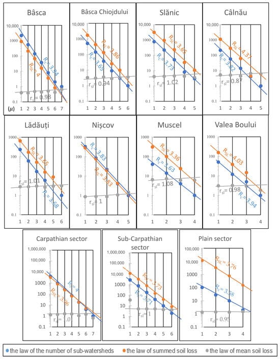
Two new morphometric relationships have been created regarding mean soil loss and summed soil loss, based on Horton’s law. The law of summed soil loss tends to exhibit an inverse geometric progression pattern, the first term being represented by the sum of mean soil loss rates of first-order watersheds and the ratio being the summed soil loss ratio (R_SL). The summed values of soil loss represent the cumulative values of mean soil loss values from sub-watersheds of successively increasing order and not the total estimated quantities of soil loss. The third series is given by the law of mean soil loss, which tends to exhibit a pattern of increasing geometric progression across successive stream orders; the first term is first-order watersheds, and the ratio is the mean soil loss ratio (r_sl) (Zăvoianu, 1978; Zăvoianu et al., 2013; Horton, 1945; Zăvoianu, 1988; Armaș, 1999;) [3,5,8,10,14]. This law is the equivalent of the law of mean stream length. For the R_c, R_SL, and r_sl ratios, we did not select reference intervals; instead, we used them as descriptive parameters. These ratios show whether consecutive-order sub-watersheds vary and how significant those variations are in the resulting dataset.

SL_s represent the theoretical soil loss value of the highest-order sub-watersheds. By analogy with the degree of completion of the stream proposed by Zăvoianu (1978) [3], this term represents a condition of concordance between the theoretical (e) situation and the calculated (c) one. Since the study uses two sets of data-estimated values (e) and calculated values (c), the source of these must be specified. The estimated values, according to Horton’s morphometric principle (measured), come from the estimates of the RUSLE2015 model. On the other hand, the calculated values are those resulting from the mathematical relationships of the model (SL_s and TSL). In other words, they are not direct measurements of the volume of soil loss through erosion, but rather indicate how closely the real situation described by morphometric laws approximates the theoretical one. Values greater than 100% indicate that the calculated value has exceeded the estimated theoretical value. However, these deviations may be associated with morphometric characteristics, as well as differences in land cover, precipitation, and lithology.

E_tot represents the total estimated soil loss due to erosion, which is obtained based on the product of specific erosion Esp (the mean soil loss estimated by RUSLE2015 and expressed in t ha⁻¹ yr⁻¹) and the watershed area (S). To ensure unit compatibility, we converted sub-watershed areas to hectares. The statistical analysis involved creating a correlation graph and determining the R² coefficient. Analyzing the relationship between mean soil loss (t ha⁻¹ yr⁻¹) and sub-watershed area (ha) of the 39 sub-watersheds can highlight the intensity of soil loss. This correlation analysis allows for the comparison of soil loss levels between watersheds of different orders (Table 1).

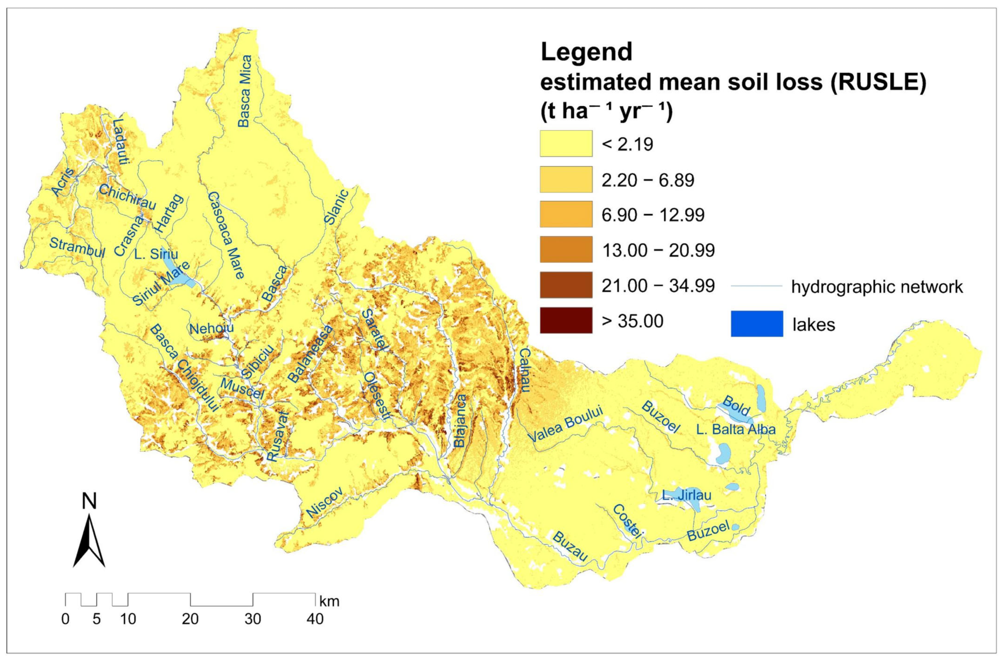
Two maps were created using the RUSLE raster. The first map presents the distribution of estimated mean soil loss across the entire Buzău Watershed. The map was classified using the Natural Breaks (Jenks) method due to the highly asymmetric distribution of the data. Through this method, each class has homogeneous values, and the differences between classes are noticeable. We extracted and grouped the pixel values according to the six created classes, from <2.19 t ha⁻¹ yr⁻¹ to >35.00 t ha⁻¹ yr⁻¹. The purpose was to see the proportion of each class of estimated mean soil loss at the basin level. In the second map, we classified the 39 sub-watersheds according to the intensity of soil loss. We classified the mean soil loss based on Panagos et al. (2015) [41], resulting in five classes.

4. Results

4.1. Sub-Watersheds Delimitation

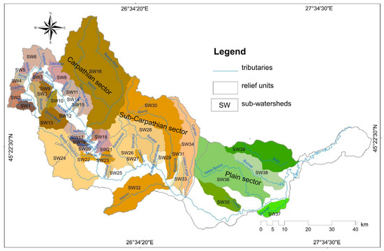
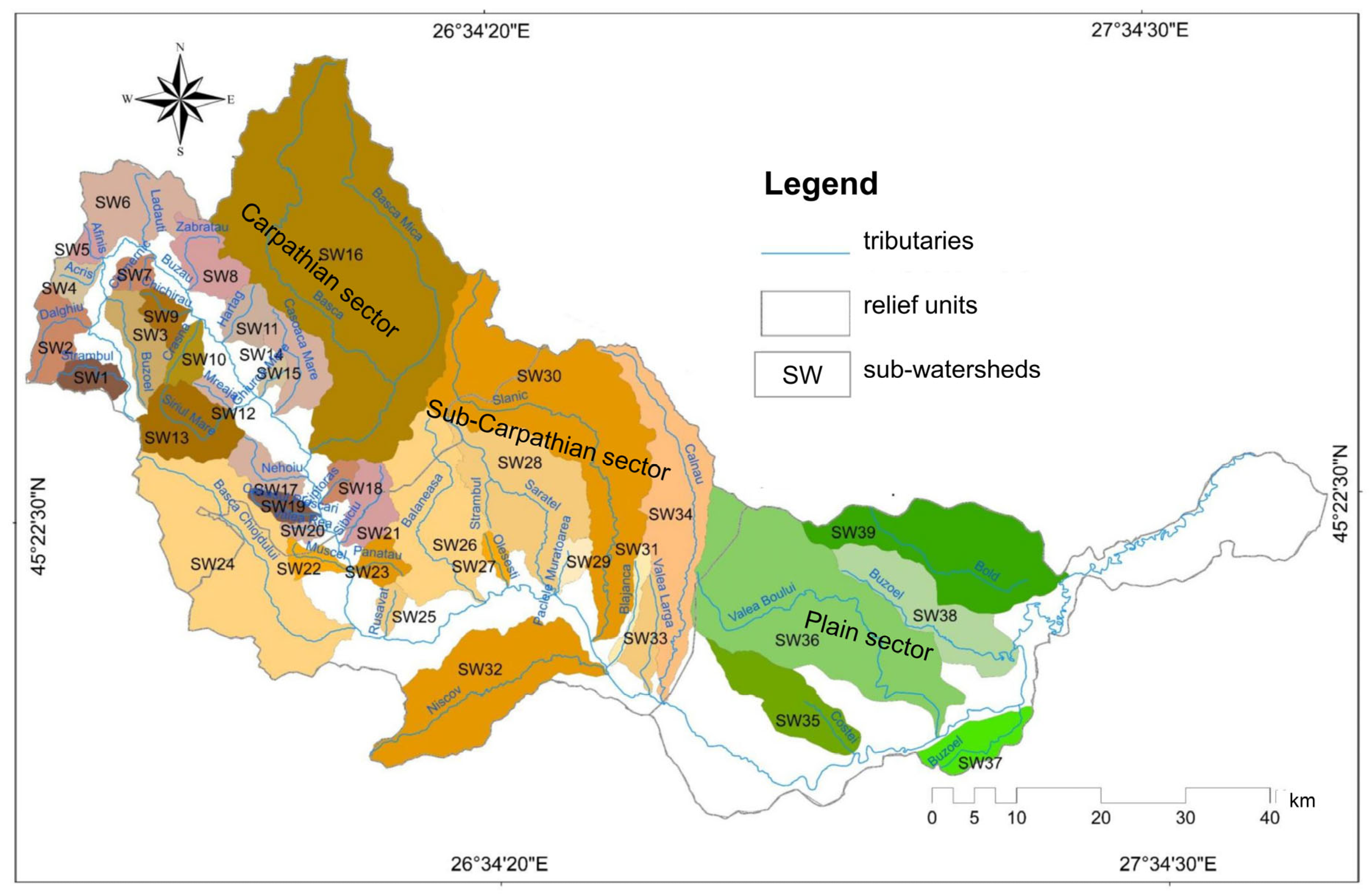
We delimited 9369 sub-watersheds of various orders. The hydrographic network was hierarchized into seven orders of streams, for which the watershed areas were delineated. The number of sub-watersheds decreases as watershed order increases. Most of the watersheds are of order 1 (6951), followed by those of order 2 (1813). Out of the 39 sub-watersheds of the main tributaries of the Buzau River, 21 have been located within the Carpathian sector, of which only Sibiciu is situated at the contact with the downstream sector. The sub-Carpathian sector contains the highest number of sub-watersheds located at the intersection with the Carpathian sector (Muscel, Bâsca Chiojdului, Bălăneasa, Sărățel, and Slănic), totaling 13. In contrast, the plain sector comprises only five sub-watersheds (Figure 3). Among these, the sub-watersheds in the Carpathian sector feature a more developed hydrographic network, with the majority reaching a stream order of 4 (48%), while the Buzoel and Lădăuți sub-watersheds reach an order of 6. Bâsca stands out as the sole sub-watershed of order 7. Downstream, the order of the stream decreases, reaching a maximum of 4 in the plain sector.

Figure 3. The map of sub-watersheds. Carpathian sector—brown; Sub-Carpathian sector—orange; Plain sector—Green.

4.2. Soil Loss Distribution Across Different-Order Sub-Watersheds

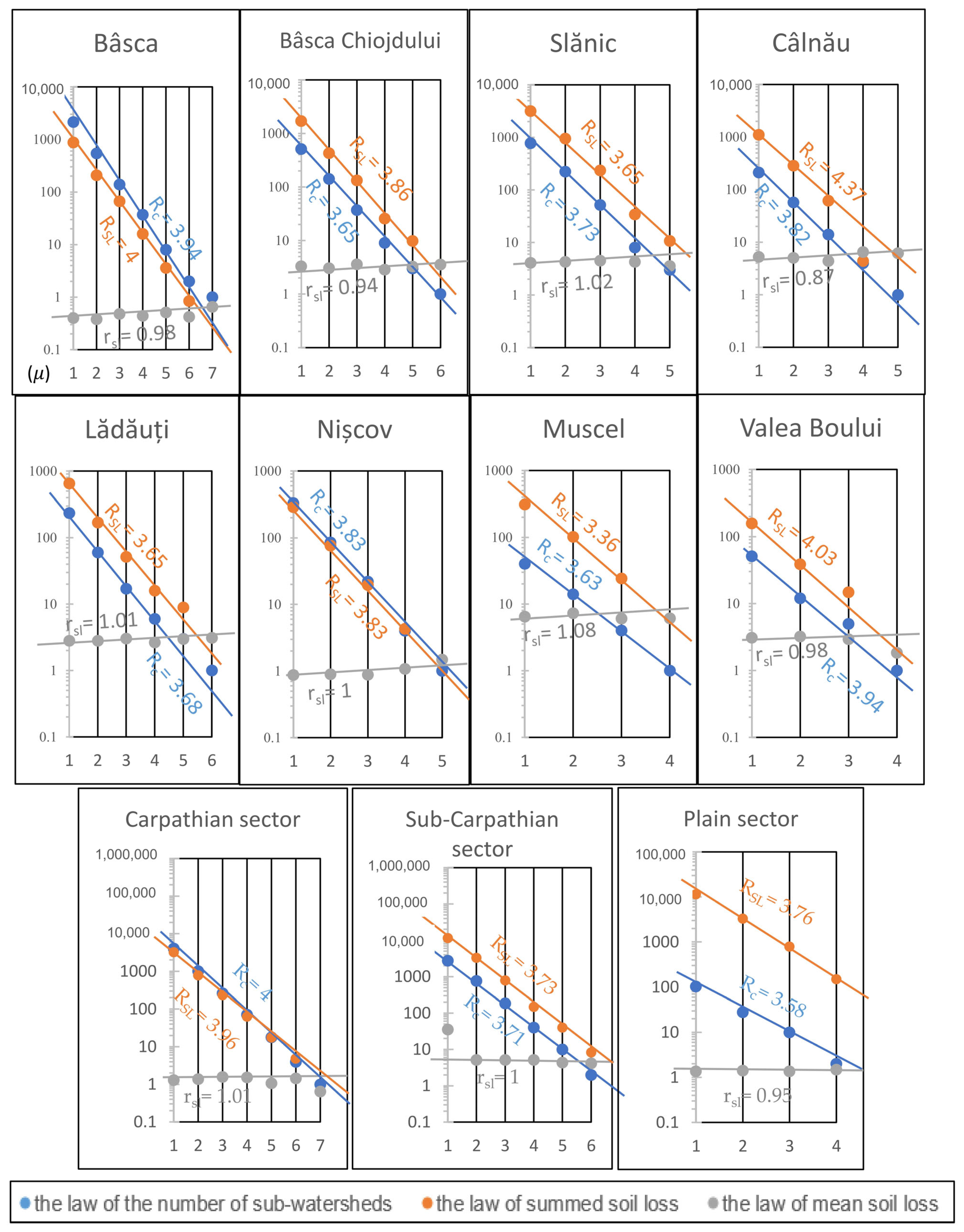
In general, the values of the law of summed soil loss closely align with a line across large spatial units (the Carpathian, sub-Carpathian, and plain sectors), as well as with certain watersheds within the sub-Carpathian sector (such as Nișcov, Slănic, Muscel, and Bâsca Chiojdului). However, deviations from the theoretical model were observed in the case of higher orders (5 and 6 for the Lădăuți watershed, or 4 for SW Câlnău and 3 for SW Valea Boului). Thus, these deviations from the straight line in the semilogarithmic system were not encountered only within a specific relief unit but can be generated by the local geomorphological conditions. Initially, the Lădăuți watershed is situated in a depression unit (the Întorsura Buzăului Depression), where the slope decreases to 9%. This trend of decreasing arrangement of data in the semilogarithmic graph has been observed, according to Horton’s laws. This approach can be used as a descriptive framework for presenting the scaling patterns of soil losses in sub-watersheds of different orders. The same relationship is encountered in the plain, specifically in the Valea Boului Watershed, where values of estimated soil loss remain relatively constant, in contrast to the sub-Carpathian sector. In the Câlnău Watershed, the SL₄ values show a negative deviation from the expected line. This suggests that the estimated soil loss is less than the expected average for this particular order.

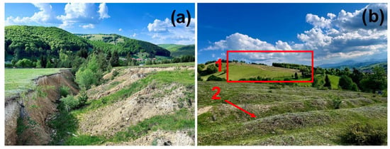
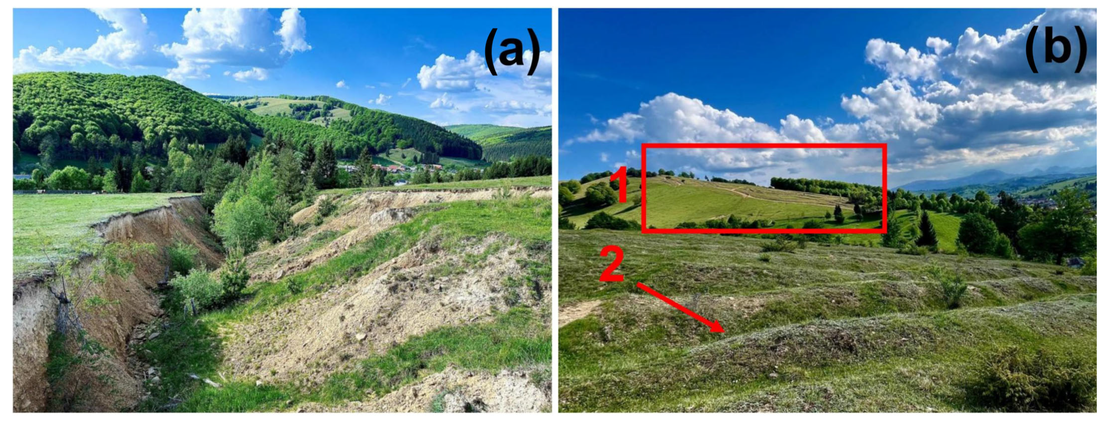
Very high values of soil loss occur locally, represented by rills and gullies, for example in the Lădăuți sub-Watershed (Figure 4). Higher-order sub-watersheds include lower-order sub-watersheds, which leads to the aggregation of the entire amount of soil loss. The larger area of the sub-watersheds does not automatically mean that the cumulative soil loss increases, as the higher-order sub-watersheds include areas where soil loss is reduced or absent.

Figure 4. Examples of soil loss due to erosion include: (a) an active torrent in the Lădăuți sub-Watershed; (b) rain-induced denudation: 1—rills and 2—gullies in the Lădăuți sub-Watershed.

The sum of the soil loss terms of the decreasing geometric progression (TSL) estimated through morphometric models (calculated) shows slight variations compared with the raw estimated values extracted from RUSLE 2015. This situation follows the pattern of the morphometric model of drainage that served as the methodological model. The sub-watersheds Zăbrătău, Mreaja, Nișcov, Valea Largă, and Buzoel (both on the right and left) show calculated values of TSL, which are close to those obtained from the raster model. These results capture the main features of the empirical pattern observed within the RUSLE dataset. Therefore, this concordance constitutes an internal verification of the consistency of the calculation, but not an independent evaluation of the empirical relationship’s performance. The good concordance between the calculated and estimated values may be determined by local conditions. For instance, the Curbicortical Flysch Nappe, which can influence the substrate’s resistance to erosion, is including to the Zăbrătău sub-Watershed. In general, the calculated values are lower than the estimated measured values, reflecting a consistent trend. Calculated values may be lower because they do not capture the heterogeneity of the relief and climatic variability, which leads to an ideal theoretical average. For example, in Câlnău, the estimated summed soil loss is 1470.73 t ha⁻¹ yr⁻¹, while the calculated value is 1440.09 t ha⁻¹ yr⁻¹ (Table S1). The smallest discrepancy occurs in the last five sub-watersheds, where the processes are slow and uniform, with the lowest recorded loss (286 t ha⁻¹ yr⁻¹). The law of mean soil loss showed good agreement with the expected theoretical relationship (r_sl = 0.95) and, particularly, for the Valea Boului sub-Watershed (r_sl = 0.98). The low values of these ratios indicate very small differences between the mean soil loss in sub-watersheds of successively increasing order. The data align closely along a straight line (Figure 5). In contrast, the ratio shows variability within the upstream sectors: the mountainous sector (r_sl = 0.53 in the Ghiurca Mare sub-Watershed and r_sl = 2.27 in Harțag) and the sub-Carpathian sector (r_sl = 0.80 in Blăjanca and r_sl = 2.63 in Valea Largă). The elevated range in the Harțag and Valea Largă sub-watersheds may suggest an increase in mean soil loss among successive-order watersheds. There are cases of doubled rates of soil loss and areas with no soil loss, leading to averaging. In the Carpathian and sub-Carpathian sectors, the R_SL is 1; this averaging tends to obscure the local variability determined by the relief and the significant soil loss that occurs over limited areas. (Table 2).

Figure 5. The morphometric model of soil loss in the sub-watersheds of the Carpathian sector (Bâsca and Lădăuți), the sub-Carpathian sector (Muscel, Bâsca Chiojdului, Slănic, Nișcov, and Câlnău), and the plain sector (Valea Boului).

Table 2. The soil loss morphometric ratios for the 39 sub-watersheds (where R_c = confluence ratio; R_SL = summed soil loss ratio; r_sl = mean soil loss ratio).

Sub-Watersheds	Rc	RSL	rsl
SW1-Strâmbul	4.21	4.03	1.04
SW2-Dălghiu	4.28	4.41	0.97
SW3-Buzoel	3.71	3.00	1.24
SW4-Acriș	5.29	6.98	0.76
SW5-Afiniș	4.00	3.74	1.07
SW6-Lădăuți	3.68	3.65	1.01
SW7-Ciumernic	3.81	3.85	0.99
SW8-Zăbrătău	3.87	3.99	0.97
SW9-Chichirău	4.14	3.99	1.04
SW10-Crasna	4.46	3.38	1.32
SW11-Harțag	4.25	1.87	2.27
SW12-Mreaja	4.63	4.92	0.94
SW13-Siriul Mare	4.45	5.07	0.88
SW14-Ghiurca Mare	4.90	9.28	0.53
SW15-Cășoaca	4.48	3.09	1.45
SW16-Bâsca	3.94	4.00	0.98
SW17-Nehoiu	3.98	3.47	1.15
SW18-Ciptoraș	3.56	4.39	0.81
SW19-Cătiașu Plescari	5.00	4.51	1.11
SW20-Valea Rea	3.90	1.95	2.00
SW21-Sibiciu	4.23	3.93	1.08
SW22-Muscel	3.63	3.36	1.08
SW23-Pănătău	3.58	3.55	1.01
SW24-Bâsca Chiojdului	3.65	3.86	0.94
SW25-Rușavăț	4.98	4.50	1.11
SW26-Bălăneasa	3.29	3.65	0.90
SW27-Oleșești	3.61	3.04	1.19
SW28-Sărățel	3.76	3.67	1.03
SW29-Pâclele Murătoarea	4.75	4.71	1.01
SW30-Slănic	3.73	3.65	1.02
SW31-Blăjanca	4.00	5.02	0.80
SW32-Nișcov	3.83	3.83	1.00
SW33-Valea Largă	10.20	3.88	2.63
SW34-Câlnău	3.82	4.37	0.87
SW35-Coștei	3.13	3.29	0.96
SW36-Valea Boului	3.94	4.03	0.98
SW37-Buzoel (r)	4.07	3.99	1.02
SW38-Buzoel (l)	2.74	2.91	0.94
SW39-Bold	3.33	2.98	1.12

4.3. Soil Loss Intensity and Watershed Hierarchization

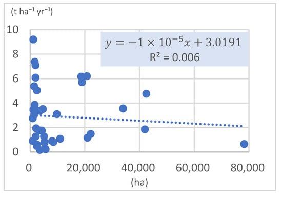
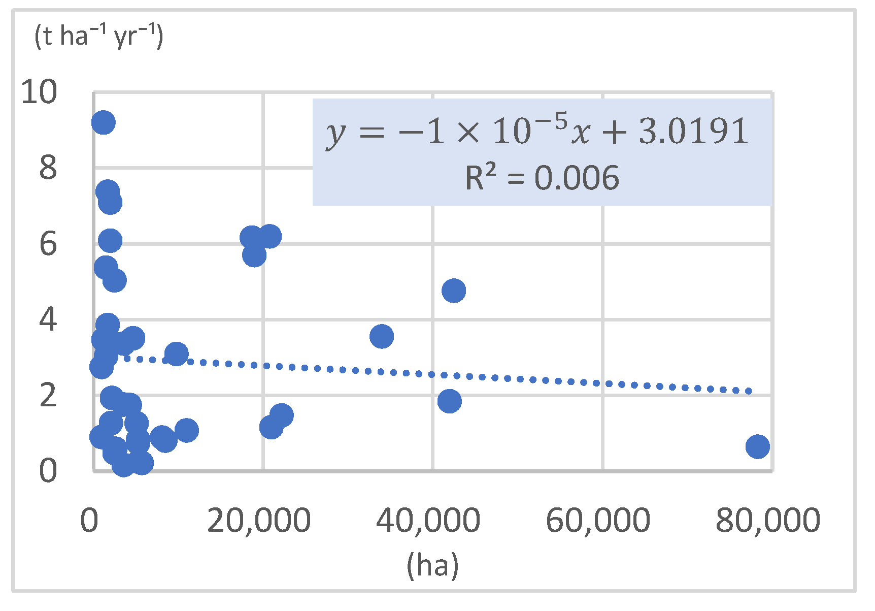
Overall, the coefficient of determination R² shows a weak relationship between soil loss intensity and watershed area (0.006). (Figure 6). Since the mean soil loss is dispersed, other local conditions could influence these values, such as lithological structure, land use, or slope. However, in the five watersheds of the plain sector, the Pearson coefficient (r) value is 0.98. The size of the watershed is not a causal predictor of soil loss by erosion but rather a valid proxy under certain conditions where the processes are more uniform. In this case, the size of the watershed is an indirect indicator involved in soil loss.

Figure 6. The correlation between soil loss intensity and area of the 39 sub-watersheds.

Although larger areas are characterized by higher values of soil loss due to erosion, the results indicate that the total estimated amount of soil loss is not directly influenced by the watershed area. The Bâsca sub-Watershed records a mean soil loss of 0.65 t ha⁻¹ yr⁻¹, which is much less than the mean soil losses from the Slănic sub-Watershed (4.76 t ha⁻¹ yr⁻¹) or the Bâsca Chiojdului sub-Watershed (3.55 t ha⁻¹ yr⁻¹). Although the Bâsca sub-Watershed has a considerable area of 78,300 ha, in contrast to the others (Slănic = 42,500 ha and Bâsca Chiojdului = 34,000 ha), a total of 50,573.86 t yr⁻¹ is lost. The Bâsca Chiojdului and Slănic sub-watersheds lose 2.4 and 4 times more than the Bâsca sub-Watershed. Therefore, they are some of the most susceptible sub-watersheds to geomorphological processes. It should be noted that in the Bâsca sub-watershed, cambisol soils predominate, while the Bâsca Chiojdului is situated in an area characterized by luvisols.

The morphological unit affects the extent of soil loss. In the case of SW11, mean soil loss is estimated at 0.16 t ha⁻¹ yr⁻¹ across an area of 3600 ha, while SW33 experiences a much higher loss of 3.36 t ha⁻¹ yr⁻¹ over the same area. The discrepancies can be attributed to the varying resistance of the rocks found in the Carpathian sector. In regions comparable with the Carpathian sector (Mreaja and Valea Rea), the Oleșești Watershed exhibits a soil loss that is approximately double the combined total for the other two sub-watersheds, reaching 9.19 t ha⁻¹ yr⁻¹ (Table S1).

The discrepancies between the relief units and the sub-watersheds, as well as within them, can be visualized. The relatively uniform soil loss rates are in the plain sector, where the slopes are reduced, and in the highest areas of the Carpathian sector. Estimated soil losses are below 2.1 t ha⁻¹ yr⁻¹.

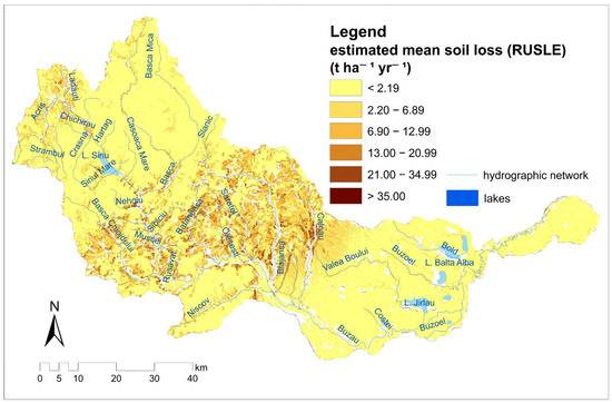
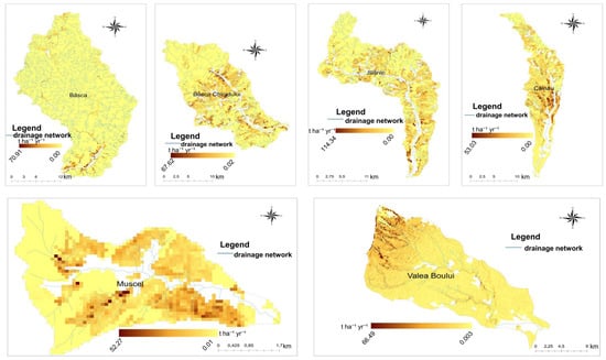
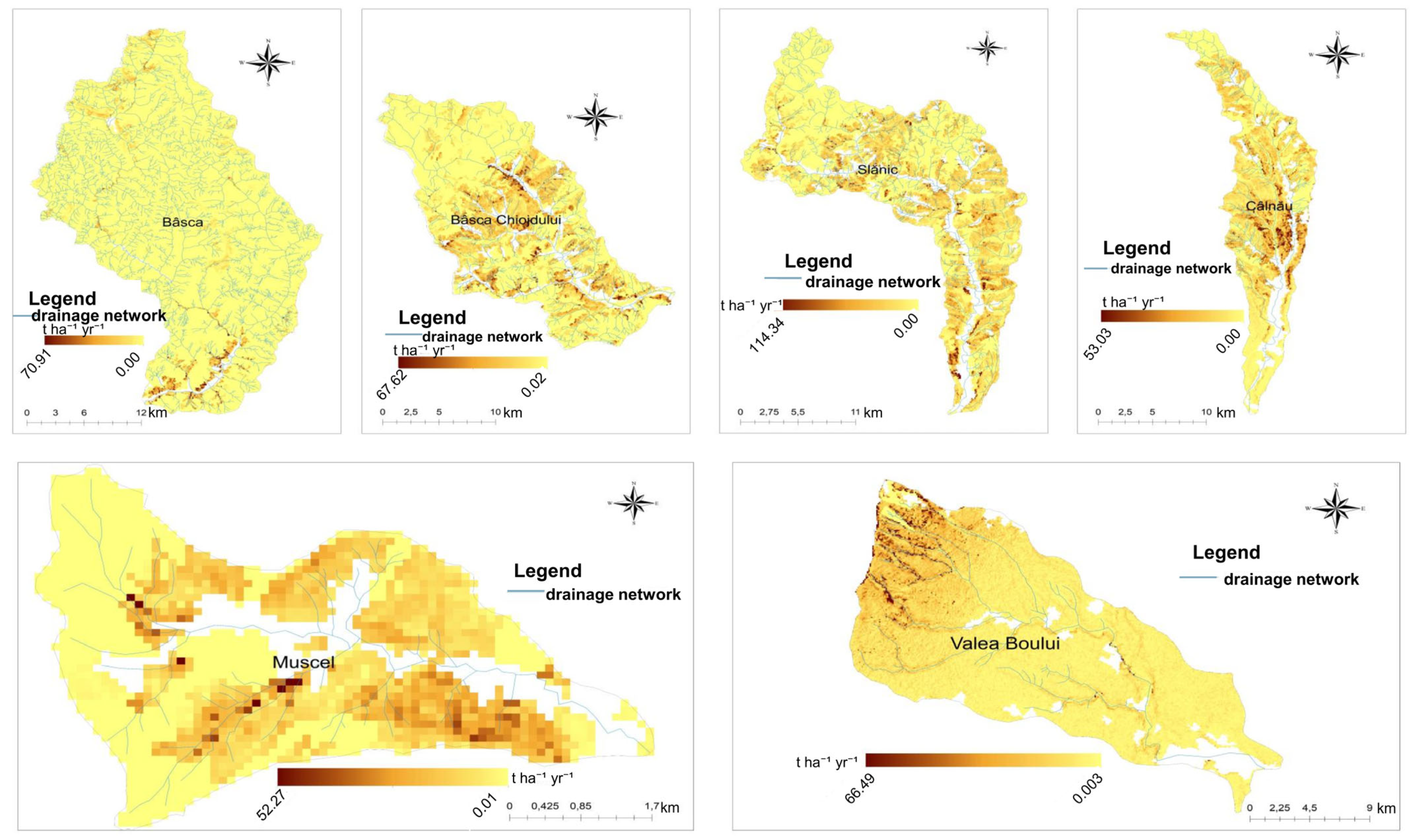
The most significant values of soil loss are observed downstream, at the confluence of Bâsca Mică and Bâsca Mare, and in the sub-watershed of Valea Boului; contact with the sub-Carpathians of Buzău leads to increased susceptibility to erosion in the upper sector. The largest area in the Buzău Watershed (76%) has low mean soil loss values, below 2.19 t ha⁻¹ yr⁻¹ (Figure 7). However, soil losses are not distributed uniformly. The Nișcov sub-Watershed is less susceptible to soil loss, although it has the largest area covered by luvisols. In contrast, the Nișcov sub-Watershed is covered by deciduous forests over an area of approximately 161.42 km², which constitutes about 73% of the watershed’s area. The sub-watersheds of Bâsca Chiojdului, Slănic, Câlnău, and Muscel have larger areas affected by soil loss due to erosion (Figure 8).

Figure 7. Geographical distribution of RUSLE2015-estimated soil loss in the Buzău River Basin (t ha⁻¹ yr⁻¹).

Figure 8. RUSLE2015-estimated soil loss distribution (t ha⁻¹ yr⁻¹) in Bâsca, Bâsca Chiojdului, Slănic, Câlnău, Muscel, and Valea Boului sub-watersheds.

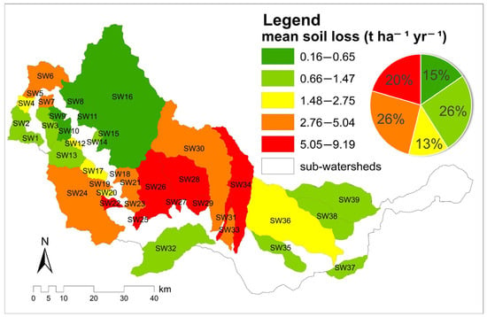
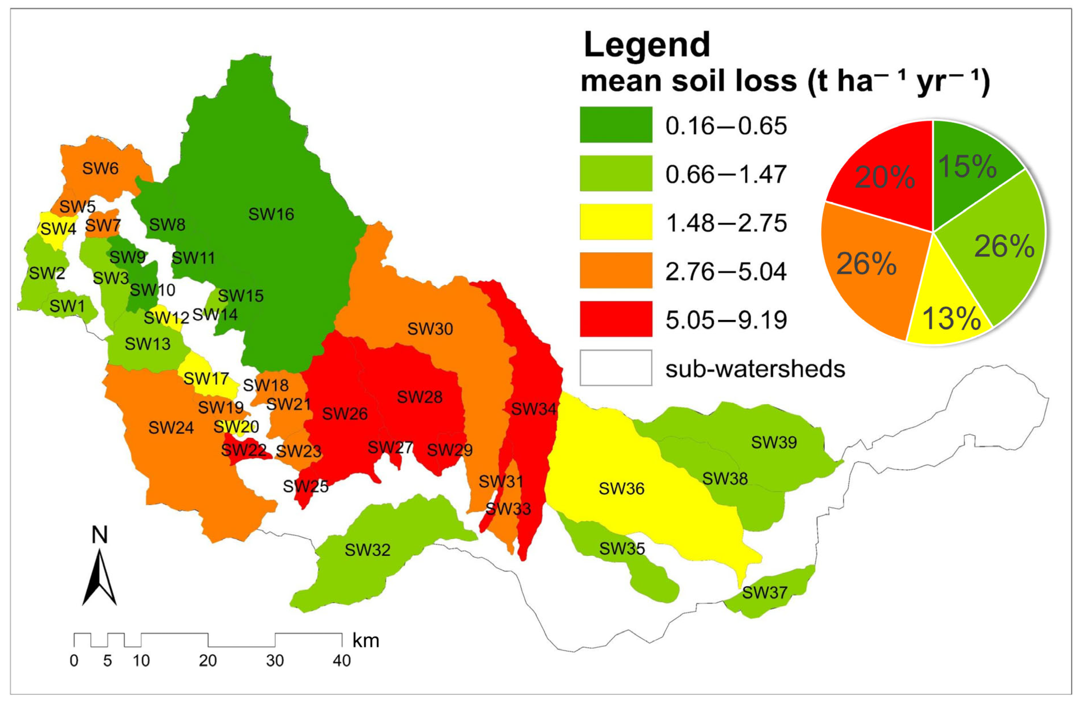
The spatial distribution of estimated mean soil loss in the 39 sub-watersheds indicates that 20% of them are susceptible to soil loss through erosion. A total of eight sub-watersheds lose over 5 t ha⁻¹ an⁻¹, all of which are located in the sub-Carpathian sector. That means about 62% of this sector. The Oleşeşti sub-Watershed is the most affected by soil loss (8%), with a mean loss of 9.19 t ha⁻¹ yr⁻¹, which amounts to approximately 11,032 t yr⁻¹, considering its area of only 12 km². A similar case is observed in the Pâclele Murătoarea sub-Watershed, where the mean soil loss is 7.08 t ha⁻¹ yr⁻¹, equivalent to approximately 14,166 t yr⁻¹, or in Blăjanca, where the mean soil loss is 7.37 t ha⁻¹ yr⁻¹, with a total loss of approximately 12,533 t yr⁻¹. The lowest intensities of soil loss (under 0.65 t ha⁻¹ yr⁻¹) are found in the Carpathian sector, within seven sub-watersheds (SW8-SW11; SW14-SW16). Unfortunately, this pattern represents only 15% of the entire Buzău Watershed.

The sub-watersheds in the lower sector exhibit low soil loss rates of less than 2.75 t ha⁻¹ yr⁻¹, with accumulation processes being more pronounced there (Figure 9).

Figure 9. The sub-watersheds distribution of soil loss intensity (based on mean RUSLE values).

The distribution of the estimated mean and total values of soil loss from the sub-watersheds corresponding to the three sectors showed that the sub-Carpathian sector is the most prone to soil loss. With an average of 5.49, the sub-Carpathian sector contributes 66% to the mean soil loss within the Buzău River Basin. Moreover, it contributes 73% to the total estimated amount of soil loss through erosion in the entire watershed. The Carpathian sector occupies 48% of the Buzău River Basin area, yet it contributes only 15% to the total soil loss, which is three percentage points more than the plain sector, which has the smallest share in the watershed (6%) and the smallest number of sub-watersheds (5).

5. Discussion

When assessing the impact of soil loss, which indicator more accurately reflects a watershed’s susceptibility to soil loss: total soil loss or the intensity of this process? Estimating soil loss using the RUSLE model involves empirically quantifying the material eroded from slopes. On the other hand, the hierarchical distribution of soil loss allows for comparisons between heterogeneous watersheds and helps identify critical areas where effective soil conservation measures are essential. A comprehensive assessment of soil loss in a watershed should consider both process intensity and spatial distribution, recognizing the complementarity of these two indicators. (Borrelli et al., 2017; Panagos et al., 2015) [35,41].

A main limitation of the study is that the analyzed values of soil loss through the RUSLE model are estimates and do not represent actual direct measurements. The 100 m spatial resolution of the raster was considered adequate for the comparative analysis of the mean of successive sub-watersheds, given the regional scale. The Buzău Basin covers an area of 5264 km². Moreover, field observations in the Lădăuți sub-Watershed have confirmed the presence of geomorphological processes (torrential forms) in areas where the spatial distribution of RUSLE-estimated soil loss indicates their presence. However, these observations do not provide a quantitative validation of the model. As a future direction, the need for direct measurements of the total amount of soil lost from sub-watersheds of different orders is being considered.

The analysis of the watershed as a whole tends to mask the spatial variability of morphometric indicators. In general, smaller sub-watersheds seem to exhibit higher soil loss rates, measured in t ha⁻¹ yr⁻¹, with the most important impact being in Oleșești (9.19 t ha⁻¹ yr⁻¹) and Blăjanca (7.37 t ha⁻¹ yr⁻¹), both located in the sub-Carpathian sector. However, the relationship between soil loss intensity and watershed area has proven to be very weak. These values of mean soil loss should be correlated with local conditions. In this sector, friable rocks (clays and marls) predominate, which are more susceptible to erosion (Constantin et al., 2013) [49], especially on slopes that lack vegetation (Prăvălie & Costache, 2014) [50] and that are subjected to agricultural practices (Niacșu et al., 2022) [51]. The high value of the Pearson coefficient (r = 0.98) at the level of the plain sector is limited by the small number of sub-watersheds (5) analyzed. This means that in the future, more detailed analyses are needed regarding the morphometric control of surfaces on soil loss in the watersheds. The presence of clay may contribute to significant soil loss in the Slănic Watershed, totaling 202,325.48 t yr⁻¹. They support the need for intervention to stabilize slopes and mitigate erosion through the creation of grassed strips (Silva et al., 2024) [52], afforestation efforts (Murătoreanu et al., 2025; Malek et al., 2015) [53,54], and the implementation of sustainable agricultural practices (Li et al., 2023) [55].

The Bâsca watershed has an estimated soil loss of about 50,573.86 t yr⁻¹ (0.65 t ha⁻¹ yr⁻¹ being the mean soil loss rate), but its value is much lower than that of several much smaller watersheds. These values can be associated with the lithology represented by the Tarcău Sandstone Facies and the degree of forest cover on the slopes.

Overall, the contact between two different units is more susceptible to soil loss. In the locality of Fundeni in the Câlnău sub-Watershed or in Gura Teghii in the Bâsca sub-Watershed, major soil losses are estimated in the proximity of the riverbeds (Gherghe et al., 2021) [56] and not at the highest altitudes. For this reason, the analysis of liquid and solid discharges becomes imperative. The pressure will be placed on the transport capacity of the eroded material, which will quickly reach the riverbed. The river’s hydrological regime will play an important role at the same time: it will either transport the solid discharge or quickly deposit it as a result of drought. Thus, the integration in a morphometric model of solid discharge would be conclusive for further analyses.

The arrangement of the summed and mean values in geometric progressions generally reproduces the patterns described by the morphometric model of drainage. Deviations from the line are supported by relief and lithology (Revuelta-Acosta et al., 2025; Chandniha & Kansal, 2017) [57,58]. A study published by Feng et al. (2020) [59] shows that the mean drained area increases geometrically with the order of the watershed, while Horton (1945) [8] and Folk (1971) [60] have demonstrated that the mean relief and mean slope of river segments decrease with the increase in order of magnitude. This method allows for the interpretation of soil loss (López-Ramos et al., 2022) [61]. Additionally, Popović et al. (2021) [62] demonstrate that solid load significantly influences the evolution of channel morphology.

Horton’s laws have been well validated in many studies conducted in heterogeneous watersheds. The semilogarithmic representation of the number of streams and the number of sub-watersheds highlight linear relationships (Charizopoulos et al., 2019) [63]. Morphometric laws do not manifest identically throughout the entire watershed, but discrepancies appear between the estimated and calculated values in some sub-watersheds in the sub-Carpathian sector, such as SW Câlnău. These deviations may suggest the possibility of the formation of new quantities of soil that are lost and, implicitly, gully erosion. The sub-watersheds in the plain sector have demonstrated the highest degree of uniformity, these results being confirmed by the principle that downstream floodplains function as sediment accumulation area, rather than loss area (Moustakidis et al., 2024) [64].

However, a limitation of the analysis is that it exclusively considers the analysis of watershed areas. Interbasin areas, which can be influenced by slope processes, should be included in the analysis, as this could alter the potential soil loss intensity and the total amount of soil loss from a particular morphological unit. Furthermore, the reliance on morphometric models only reflects the organization of soil loss at the sub-watersheds level, without capturing the temporal variability of erosion processes. In reality, soil loss tends to be episodic and predominantly occurs during intense, short-duration rainfall events that account for the majority of annual soil losses (Panagos et al., 2015) [41]. It becomes necessary to extend the analysis by graphically representing parameters such as the amount of precipitation and deforestation carried out in sub-watersheds of various orders. These could capture local variations between sub-watersheds and provide a clear understanding of the susceptibility to the formation of torrential forms.

The differences between the distribution of mean soil loss estimated at the Buzău Watershed level and those at the sub-watersheds level are the result of spatial aggregation. A watershed can include a high number of cells with low values, and the presence of outliers can result in classification into an intermediate category, as is the case with the Valea Boului sub-Watershed. Although it generally exhibits mean soil losses of less than 2.19 t ha⁻¹ yr⁻¹, the high values at the contact with the sub-Carpathian sector place it in the moderate intensity class, indicated in yellow. Thus, another limitation is related to the emergence of internal spatial heterogeneity within the pixels, which causes the phenomenon of extreme value eclipsing (Pastor et al., 2024) [42].

As previously mentioned, it is essential not only to assess the quantity of soil loss but also to evaluate the transport capacity of sediments that are evacuated through the hydrographic network. As a future direction, integrating the morphometric model of both liquid and solid discharges would be beneficial. There exist interdependent relationships between the hydrological regime and erosion processes, and while the presence of hydrotechnical infrastructure (bridges and dams) does not eliminate the risk, it serves only to mitigate it (Popa et al., 2019) [65].

6. Conclusions

This study analyzed the hierarchical distribution of RUSLE-estimated mean soil loss in the 39 sub-watersheds of the Buzău River Basin. Starting from the morphometric laws and the morphometric drainage model, we developed a new morphometric model of soil loss, using values extracted from the RUSLE2015 model. We have observed that the summed and mean soil loss laws tended to exhibit successive geometric progression patterns. The estimated soil loss rate tends to decrease with increasing sub-watershed order. In general, the values showed a good alignment with the expected line in most of the analyzed sub-watersheds. Slight deviations to the left have been observed for the higher order of the Lădăuți, Câlnău, and Valea Boului sub-watersheds. The positioning in different relief units may support the idea that these deviations are the result of local conditions. A value of R_SL of 1 diminishes the local variability of the estimated soil losses. The analysis of the successive distribution by sub-watersheds order has determined variations of this ratio in sub-watersheds from the Carpathian and sub-Carpathian sectors.

The watershed area does not explain these variations; the determination coefficient Rp of 0.006 indicates a weak linear relationship between the two parameters. Sub-watersheds with similar areas recorded different rates of mean and total soil loss. For example, SW 11 recorded mean losses of 0.16 t ha⁻¹ yr⁻¹, while SW 33 recorded 3.36 t ha⁻¹ yr⁻¹. Oleșești recorded the highest value of mean soil loss at 9.19 t ha ⁻¹ yr ⁻¹, double the value of the Mreaja and Valea Rea sub-watersheds, whose areas are comparable. Moreover, the Slănic sub-watershed loses a total of 202,325.48 t yr⁻¹ over an area of 42,500 ha, while Bâsca loses only 50,573.86 t yr⁻¹. A main finding was the assignment of these sub-watersheds within the sub-Carpathian sector.

A total of 76% of the Buzău Watershed area shows low values of the estimated mean soil loss, below 2.19 t ha ⁻¹ yr ⁻¹. However, the distribution of mean soil loss is heterogeneous. The sub-Carpathian sector contributes 66% to the mean soil loss and 73% to the total soil loss at the overall level. A total of 20% of the sub-watersheds show mean losses of over 5.05 t ha ⁻¹ yr ⁻¹ and are classified into this sector.

This study presents some limitations regarding the RUSLE raster resolution and how it was clipped according to the sub-watershed boundaries. The 100 m spatial resolution and the non-conformity with sub-watershed boundaries may not capture local variations determined by the heterogeneity of the relief. However, we have tracked the organization of mean and cumulative soil losses between sub-watersheds of successively increasing order. It should be noted that the soil loss values are estimated using the RUSLE model and do not constitute direct measurements of the actual amount of soil lost from the watershed.

We need to explore future directions for validation regarding the validation of the model through direct measurements of the actual amount of soil lost from the watershed. Testing the model on other heterogeneous watersheds could verify whether the morphometric laws follow the same pattern of geometric organization. In conclusion, the soil losses estimated by RUSLE are organized similarly to the morphometric characteristics of the drainage network, forming successive geometric ratios and progressions by order of sub-watershed. This study provides a descriptive framework for the organization and comparison of estimated soil loss across different sub-watersheds and geographical sectors. It should not be interpreted as an assessment of current conditions. However, it can serve as an analytical tool for planning soil conservation measures and as a reference in subsequent investigations.

References

- Gâștescu, P.; Murărescu, O.; Brețcan, P.; Dinu, I. Hidrologie Generală-Lucrări Practice [General Hydrology-Practical Exercises]; Transversal: Târgoviște, Romania, 2006. [Google Scholar]
- Posea, G. Geomorfologia României [Geomorphology of Romania]; Fundației România de Mâine: București, Romania, 2005. [Google Scholar]
- Zăvoianu, I. Morfometria Bazinelor Hidrografice. [Morphometry of Drainage Basins]; Academiei Republicii Socialiste România: București, Romania, 1978. [Google Scholar]
- Clarke, J.I. Morphometry from Maps. In Essays in Geomorphology; Dury, G.H., Ed.; Elsevier: New York, NY, USA, 1966; pp. 235–274. [Google Scholar]
- Zăvoianu, I.; Cruceru, N.; Herişanu, G. Morphometry elements of hydrographic basins with use in the characterization of relief characterization of relief. Rev. Geomorfol. 2013, 15, 89–98. [Google Scholar]
- Demoulin, A. Basin and river profile morphometry: A new index with a high potential for relative dating of tectonic uplift. Geomorphology 2011, 126, 97–107. [Google Scholar] [CrossRef] [Scilit]
- Horton, R.E. Drainage basin characteristics transactions. Am. Geophys. Union 1932, 13, 350–361. [Google Scholar] [CrossRef] [Scilit]
- Horton, R.E. Erosional development of streams and their drainage basin; hydrophysical approach to quantitative morphology. Geol. Soc. Am. Bull. 1945, 56, 151–180. [Google Scholar] [CrossRef] [Scilit]
- Strahler, A.N. Hypsometric analysis (area-altitude) of erosional topography. Geol. Soc. Am. Bull. 1952, 63, 117–142. [Google Scholar] [CrossRef] [Scilit]
- Armaş, I. Bazinul Hidrografic Doftana: Studiu de Geomorfologie [The Doftana River Basin: A Geomorphological Study]; Enciclopedică: București, Romania, 1999. [Google Scholar]
- Marinescu, E. Morphometrical and morphographical features of the Gilort hydrographical basin/Caracteristici morfometrice si morfografice ale bazinului Gilort. Forum Geogr. 2007, 6, 88–101. [Google Scholar]
- Codreanu, I. Utilizarea modelelor matematice în caracterizarea morfometriei bazinilor râurilor Soloneț și Cogâlnic. Bul. Institutului Geol. Seismol. AŞM 2017, 1, 71–78. [Google Scholar]
- Zăvoianu, I.; Herișanu, G.; Marin, C.; Cruceru, N.; Parichi, M.; Vartolomei, F. Relații Cantitative Între Producția de Aluviuni în Suspensie și Factorii de Mediu [Quantitative Relationships Between Suspended Sediment Yield and Environmental Factors]; Transversal: București, Romania, 2011. [Google Scholar]
- Zăvoianu, I. Morphometrical model of average mean channel slope in the Buzău Subcarpathians. Rev. Roum. Geol. Geophys. Geogr. Série Geogr. 1998, 32, 37–42. [Google Scholar]
- Cruceru, N. Bazinul Sărățel: Studiu de Geomorfologie [The Sărățel River Basin: A Geomorphological Study]; Editura Transversal: Târgoviște, Romania, 2011. [Google Scholar]
- Cruceru, N.; Herișanu, G. The Codification of the Rivers Network and Basins from the Sărățel Morpho-Hydrographic System (Buzău). Lucr. Semin. Geogr. Dimitrie Cantemir 2011, 31, 81–88. [Google Scholar]
- Grecu, F. Bazinul Hârtibaciu. Elemente de Morfohidrografie [Hârtibaciu Basin. Elements of Morphohydrography]; Academiei Române: Bucureşti, Romania, 1992. [Google Scholar]
- Minea, G. Bazinul Hidrografic al Râului Bâsca: Studiu de Hidrogeografie [The Bâsca River Basin: A Hydrogeographical Study]; Universității din București: București, Romania, 2012. [Google Scholar]
- Minea, G. Assessment of the flash flood potential of Bâsca river catchment (Romania) based on physiographic factors. Open Geosci. 2013, 5, 344–353. [Google Scholar] [CrossRef] [Scilit]
- Minea, I.S. Râurile Bazinului Buzău. Consideraţii Hidrografice şi Hidrologice [Rivers of Buzău Basin. Hydrographic and Hydrological Considerations]; Alpha MDN: Buzău, Romania, 2011. [Google Scholar]
- Vîrghileanu, M.; Săvulescu, I.; Mihai, B.A.; Bizdadea, C.G.; Paraschiv, M.G. RUSLE-Based Scenarios for Sustainable Soil Management: Case Studies from Romanian Subcarpathians. Eur. J. Soil Sci. 2024, 75, e13526. [Google Scholar] [CrossRef] [Scilit]
- Vîrghileanu, M.; Șandric, I.; Mihai, B.A.; Săvulescu, I.; Bizdadea, C.G. Comparative Assessment of Vegetation Cover and Management Factor in Soil Loss Modelling Using Sentinel-2 MSI Time-Series Imagery: A case study from the Romanian Carpathian-Subcarpathian region. Remote Sens. Appl. Soc. Environ. 2026, 42, 102013. [Google Scholar] [CrossRef] [Scilit]
- Rizac, A.; Șandric, I.; Comănescu, L. Revised Universal Soil Loss Equation (Rusle) Model in the Bâsca Chiojdului River Basin (subcarpathians, Romania). Carpathian J. Earth Environ. Sci. 2025, 20, 373–384. [Google Scholar] [CrossRef] [Scilit]
- Patriche, C.V. Soil Erosion Assessment in Romania under Current and Future Climate Conditions Using the RUSLE Model. Geoderma Reg. 2023, 34, e00687. [Google Scholar] [CrossRef] [Scilit]
- Prăvălie, R.; Necula, N.; Borrelli, P.; Tișcovschi, A.; Săvulescu, I. A Complex Spatial Inventory of Land Degradation and Desertification in Romania. Ecol. Indic. 2025, 174, 113548. [Google Scholar] [CrossRef] [Scilit]
- Nistor, C.; Săvulescu, I.; Ioana-Toroimac, G.; Carablaisă, S. Exploring soil erosion and reservoir sedimentation through the RUSLE model and bathymetric survey. Int. Soil Water Conserv. Res. 2025, 13, 235–247. [Google Scholar] [CrossRef] [Scilit]
- Alewell, C.; Borrelli, P.; Meusburger, K.; Panagos, P. Using the USLE: Chances, challenges and limitations of soil erosion modelling. Int. Soil Water Conserv. Res. 2019, 7, 203–225. [Google Scholar] [CrossRef] [Scilit]
- Tilman, D.; Balzer, C.; Hill, J.; Befort, B.L. Global Food Demand and the Sustainable Intensification of Agriculture. Proc. Natl. Acad. Sci. USA 2011, 108, 20260–20264. [Google Scholar] [CrossRef] [Scilit]
- Panagos, P.; Van Liedekerke, M.; Borrelli, P.; Köninger, J.; Ballabio, C.; Orgiazzi, A.; Lugato, E.; Liakos, L.; Hervas, J.; Jones, A.; et al. European Soil Data Centre 2.0: Soil data and knowledge in support of the EU policies. Eur. J. Soil Sci. 2022, 73, e13315. [Google Scholar] [CrossRef] [Scilit]
- Food and Agriculture Organization of the United Nations (FAO). Food Loss and Waste Database; FAO: Rome, Italy, 2022; Available online: https://www.fao.org/food-loss-and-food-waste/en/ (accessed on 20 June 2026).
- Andualem, T.G.; Hewa, G.A.; Myers, B.R.; Peters, S.; Boland, J. Erosion and sediment transport modeling: A systematic review. Land 2023, 12, 1396. [Google Scholar] [CrossRef] [Scilit]
- Zhao, T.; Zhou, G.G.D.; Sun, Q.; Crosta, G.B.; Song, D. (Slope erosion induced by surges of debris flow: Insights from field experiments. Landslides 2022, 19, 2367–2377. [Google Scholar] [CrossRef] [Scilit]
- Senapati, U.; Das, T.K. Assessment of Potential Land Degradation in Akarsa Watershed, West Bengal, Using GIS and Multi-Influencing Factor Technique. In Gully Erosion Studies from India and Surrounding Regions; Shit, P.K., Pourghasemi, H.R., Bhunia, G.S., Eds.; Springer International Publishing: Cham, Switzerland, 2019; pp. 187–205. [Google Scholar] [CrossRef] [Scilit]
- Prăvălie, R.; Niță, I.A.; Patriche, C.; Niculiță, M.; Birsan, M.V.; Roșca, B.; Bandoc, G. Global changes in soil organic carbon and implications for land degradation neutrality and climate stability. Environ. Res. 2021, 201, 111580. [Google Scholar] [CrossRef] [Scilit]
- Borrelli, P.; Robinson, D.A.; Fleischer, L.R.; Lugato, E.; Ballabio, C.; Alewell, C.; Meusburger, K.; Modugno, S.; Schutt, B.; Ferro, V.; et al. An assessment of the global impact of 21st-century land use change on soil erosion. Nat. Commun. 2017, 8, 2013. [Google Scholar] [CrossRef] [Scilit]
- Piacentini, T.; Galli, A.; Marsala, V.; Miccadei, E. Analysis of soil erosion induced by heavy rainfall: A case study from the NE Abruzzo Hills area in Central Italy. Water 2018, 10, 1314. [Google Scholar] [CrossRef] [Scilit]
- Wischmeier, W.H.; Smith, D.D. Predicting Rainfall Erosion Losses: A Guide to Conservation Planning; U.S. Department of Agriculture, Agriculture Handbook No. 537; USDA: Washington, DC, USA, 1978. [Google Scholar]
- Renard, K.G.; Foster, G.R.; Weesies, G.A.; McCool, D.K.; Yoder, D.C. Predicting Soil Erosion by Water: A Guide to Conservation Planning with the Revised Universal Soil Loss Equation (RUSLE); U.S. Department of Agriculture, Agriculture Handbook No. 703; USDA: Washington, DC, USA, 1997. [Google Scholar]
- Choudhury, B.U.; Nengzouzama, G.; Islam, A. Evaluation of climate change impact on soil erosion in the integrated farming system based hilly micro-watersheds using Revised Universal Soil Loss Equation. CATENA 2022, 214, 106306. [Google Scholar] [CrossRef] [Scilit]
- Borrelli, P.; Diodato, N.; Panagos, P. Rainfall erosivity in Italy: A national scale spatio-temporal assessment. Int. J. Digit. Earth 2016, 9, 835–850. [Google Scholar] [CrossRef] [Scilit]
- Panagos, P.; Borrelli, P.; Meusburger, K.; Alewell, C.; Lugato, E.; Montanarella, L. Estimating the soil erosion cover-management factor at the European scale. Land Use Policy 2015, 48, 38–50. [Google Scholar] [CrossRef] [Scilit]
- Pastor, I.; Tanislav, D.; Nedelea, A.; Dunea, D.; Serban, G.; Haghighi, A.T.; Sabau, D.; Bretcan, P. Morphometric Analysis and Prioritization of Sub-Watersheds Located in Heterogeneous Geographical Units-Case Study: The Buzău River Basin. Sustainability 2024, 16, 7567. [Google Scholar] [CrossRef] [Scilit]
- Zăvoianu, Z. Morphometry of Drainage Basins; Developments in Water Science; Elsevier: Amsterdam, The Netherlands, 1985. [Google Scholar]
- Institutul de Meteorologie și Hidrologie (IMH). Atlasul Cadastrului Apelor din România [Atlas of the Water Cadastre of Romania]; IMH: București, România, 1992. [Google Scholar]
- Micu, M. Alunecările de Teren din Carpații și Subcarpații Buzăului. STUDIU Geomorfologic [Landslides in the Buzău Carpathians and Subcarpathians: A Geomorphological Study]; Universitară: București, Romania, 2010. [Google Scholar]
- Administrația Națională “Apele Române” (ANAR). Sub-Basins (Hydrography Dataset). data.gov.ro. Available online: https://data.gov.ro/ro/dataset/hidrografie (accessed on 20 June 2026).
- European Commission, Joint Re0073earch Centre. Soil Erosion by Water (RUSLE2015) [Dataset]. Available online: https://data.jrc.ec.europa.eu/dataset/jrc-esdac-99 (accessed on 20 June 2026).
- Napoli, M.; Cecchi, S.; Orlandini, S.; Mugnai, G.; Zanchi, C.A. Simulation of field-measured soil loss in Mediterranean hilly areas (Chianti, Italy) with RUSLE. Catena 2016, 145, 246–256. [Google Scholar] [CrossRef] [Scilit]
- Constantin, M.; Bednarik, M.; Jurchescu, M.C.; Ishida, K.; Higuchi, K. Regional and Local Approaches on Landslide Susceptibility Assessment in the Region Located between the Buzău and the Slănicul Buzăului Valleys, Romania. In Landslide Science and Practice; Margottini, C., Canuti, P., Sassa, K., Eds.; Springer: Berlin/Heidelberg, Germany, 2013; pp. 365–370. [Google Scholar] [CrossRef] [Scilit]
- Prăvălie, R.; Costache, R. The potential of water erosion in Slănic River basin. Rev. Geomorfol. 2014, 16, 79–88. [Google Scholar]
- Niacșu, L.; Bucur, D.; Ioniță, I.; Codru, I.C. Soil conservation measures on degraded land in the Hilly Region of Eastern Romania: A case study from Puriceni-Bahnari Catchment. Water 2022, 14, 525. [Google Scholar] [CrossRef] [Scilit]
- Silva, T.P.; Bressiani, D.; Ebling, É.D.; Reichert, J.M. Best management practices to reduce soil erosion and change water balance components in watersheds under grain and dairy production. Int. Soil Water Conserv. Res. 2024, 12, 121–136. [Google Scholar] [CrossRef] [Scilit]
- Murătoreanu, G.; Dunea, D.; Tanislav, D.; Reid, M.; Diaconu, D.C.; Costache, A.; Pastor, I.; Brețcan, P. Soil erosion susceptibility assessment in the Bistrița River basin (Romania) using machine learning algorithms and GIS. Sci. Rep. 2025, 15, 44381. [Google Scholar] [CrossRef] [Scilit]
- Malek, Ž.; Boerboom, L.; Glade, T. Future forest cover change scenarios with implications for landslide risk: An example from Buzau Subcarpathians, Romania. Environ. Manag. 2015, 56, 1228–1243. [Google Scholar] [CrossRef] [Scilit]
- Li, C.; Lu, T.; Wang, S.; Xu, J. Coupled thorens and soil conservation service models for soil erosion assessment in a loess plateau watershed, China. Remote Sens. 2023, 15, 803. [Google Scholar] [CrossRef] [Scilit]
- Gherghe, A.; Dobre, R.R.; Apotrosoaei, V.; Briceag, A.; Melinie-Dobrinescu, M. The Bâsca Rozilei river drainage model, Romanian Carpathian belt. Geo-Eco-Marina 2021, 27, 37–54. [Google Scholar] [CrossRef]
- Revuelta-Acosta, J.D.; Garrido-Meléndez, J.; Conde-Gutiérrez, R.A.; Alcalá-Perea, G. Comprehensive geospatial assessment: Morphometric parameters and hydrological implications in five Mexican basins. Sci. Rep. 2025, 15, 21698. [Google Scholar] [CrossRef] [Scilit]
- Chandniha, S.K.; Kansal, M.L. Prioritization of sub-watersheds based on morphometric analysis using geospatial technique in Piperiya watershed, India. Appl. Water Sci. 2017, 7, 329–338. [Google Scholar] [CrossRef] [Scilit]
- Feng, M.; Jung, K.; Kim, J.C. Geomorphologic analysis of small river basin within the framework of fractal tree. Water 2020, 12, 2480. [Google Scholar] [CrossRef] [Scilit]
- Fok, Y.-S. Law of Stream Relief in Horton’s Stream Morphological System. Water Resour. Res. 1971, 7, 201–203. [Google Scholar] [CrossRef] [Scilit]
- López-Ramos, A.; Medrano-Barboza, J.P.; Martínez-Acosta, L.; Acuña, G.J.; Remolina López, J.F.; López-Lambraño, A.A. (Assessment of morphometric parameters as the basis for hydrological inferences in water resource management: A case study from the sinú river basin in Colombia. ISPRS Int. J. Geo-Inf. 2022, 11, 459. [Google Scholar] [CrossRef] [Scilit]
- Popović, P.; Devauchelle, O.; Abramian, A.; Lajeunesse, E. Sediment load determines the shape of rivers. Proc. Natl. Acad. Sci. USA 2021, 118, e2111215118. [Google Scholar] [CrossRef] [Scilit]
- Charizopoulos, N.; Mourtzios, P.; Psilovikos, T.; Psilovikos, A.; Karamoutsou, L. Morphometric analysis of the drainage network of Samos Island (northern Aegean Sea): Insights into tectonic control and flood hazards. Comptes Rendus. Géosci. 2019, 351, 375–383. [Google Scholar] [CrossRef] [Scilit]
- Moustakidis, I.D.V.; Schilling, K.E.; Weber, L.J. River floodplains as source or sink for fine sediment and total phosphorus export in an agricultural watershed. Earth Surf. Process. Landf. 2024, 49, 2677–2689. [Google Scholar] [CrossRef] [Scilit]
- Popa, M.C.; Peptenatu, D.; Drăghici, C.C.; Diaconu, D.C. Flood hazard mapping using the flood and flash-flood potential index in the Buzău River catchment, Romania. Water 2019, 11, 2116. [Google Scholar] [CrossRef] [Scilit]
Disclaimer/Publisher’s Note: The statements, opinions and data contained in all publications are solely those of the individual author(s) and contributor(s) and not of MDPI and/or the editor(s). MDPI and/or the editor(s) disclaim responsibility for any injury to people or property resulting from any ideas, methods, instructions or products referred to in the content. |
© 2026 by the authors. Licensee MDPI, Basel, Switzerland. This article is an open access article distributed under the terms and conditions of the Creative Commons Attribution (CC BY) license.