


Abstract
When considering the adsorption effect, traditional experimental methods have faced significant challenges in obtaining the solute transport parameters for composite pollutants. Based on the adsorption test data of three types of composite pollutants collected from the Web of Science and China National Knowledge Infrastructure databases from 2014 to 2024, this study employed four commonly used machine learning models, that is, Random Forest (RF), Support Vector Machine (SVM), Back Propagation Neural Network (BPNN), and Decision Tree (DT) models, to establish adsorption isotherms of pollutants with liquid-phase equilibrium concentration as the horizontal coordinate and solid-phase adsorption capacity as the vertical coordinate, and systematically investigated the adsorption characteristics of combined pollutants in the porous aquifer. Subsequently, the Mean Square Errors (MSEs) and coefficients of determination, two commonly used evaluation metrics for regression models in machine learning, were chosen to estimate the prediction effect of datasets. Combined with the convection–diffusion equation, the adsorption kinetic parameters under the mutual interference of composite pollutants, namely, the retardation factor, were solved. The results show that for the adsorption isotherms of heavy metal composite pollutants, organic composite pollutants, and heavy metal and organic combined composite pollutants, SVM, BPNN, and RF models have the best prediction effect, respectively, and their MSEs are 0.032, 0.001, and 0.018. The adsorption isotherm fitting results indicate that the heavy metal composite pollutants and organic composite pollutants conform to the Freundlich model. The retardation factor of organic composite pollutants is significantly higher than that of heavy metal composite pollutants.
1. Introduction
In recent years, groundwater in porous aquifers has faced a serious threat from composite pollutants. For instance, the results of a groundwater quality investigation conducted in a certain city in the Huaibei Plain, Anhui Province, China, revealed that the local groundwater is mainly subject to the combined pollution of heavy metal ions such as iron and manganese, as well as organic pollutants such as polycyclic aromatic hydrocarbons, phthalate esters, and dichloromethane [1,2]. Once contaminated groundwater enters the human body, it may adversely affect human health. Therefore, it is of great significance to study the migration rules of multiple pollutants in groundwater to ensure the safety of groundwater resources and human health.
Adsorption plays a key role in the migration of composite pollutants into groundwater. Current studies suggest that the adsorption mechanism of heavy metals is not fully understood. Some scholars have proposed using linear isothermal adsorption models to describe heavy metal adsorption [3], while others have emphasized the need to consider complex adsorption in addition to isothermal adsorption [4]. Moreover, complex interactions exist between different organic pollutants and between organic and heavy metal pollutants, including adsorption, desorption, fixation, and migration, which can alter the form and concentration of pollutants [5]. In porous aquifers, the combination of pollutants varies in different regions, with some regions having only two pollutants, such as iron and manganese, whereas others may have multiple coexisting pollutants, such as iron, manganese, and naphthalene. Therefore, the migration of composite pollutants in porous aquifers is influenced not only by mutual interference among pollutants but also by physical and chemical reactions between pollutants and soil particles [6,7], which greatly complicates the study of the migration laws of pollutants.
Currently, solute transport models are widely used to describe the migration of composite pollutants [8,9,10]. Among them, the convection–diffusion equation is a classical and fundamental model for studying solute transport in porous media. The retardation factor, a parameter of adsorption kinetics within this equation, reflects the adsorption–desorption characteristics of composite pollutants. It is related to the solid-phase adsorption capacity and liquid-phase concentration of pollutants and is influenced by multiple factors such as pH, water temperature, and solute type [11,12]. The retardation factor is typically obtained through experimental methods. However, with the deepening of research, the mapping relationship between model parameters and response shows stronger nonlinearity, and the requirements for the accuracy of model parameters are also increasing [13]. Therefore, traditional experimental methods face many challenges when obtaining these parameters. In previous studies, the parameters of the solute transport model are often obtained by porous medium column tests [14,15], while the experimental results were easily affected by factors such as test conditions and the proficiency of the test personnel. Moreover, the experimental methods are costly and greatly affected by interfering factors such as the regional scale, making it difficult to guarantee the accuracy of the obtained parameters.
Given the limitations of traditional experimental approaches, many scholars have sought alternative methods for estimating solute transport parameters [16,17]. Among these, machine learning methods have gradually emerged in groundwater solute transport studies because of their low computational cost and strong generalization ability, which provides an effective framework for mapping the complex relationships between various input parameters and output variables [18,19]. With the diversity of algorithm selection and strong processing capabilities for large datasets, machine learning has demonstrated great potential for the prediction of groundwater parameters. It can overcome the difficulties caused by variable terrain, complex hydrogeological features, and limited data, and has played an important role in predicting the variation in groundwater level and reserves, providing strong support for solving the shortage of water resources [20,21,22]. During the training process, the machine learning model can effectively analyze the nonlinear relationships among numerous characteristic variables that affect the parameter values. Based on the extraction of data points, hydrogeological conditions were identified, and the groundwater level was predicted [23,24], which greatly reduced the experimental time and cost, improved the research efficiency, and solved the limitations of traditional groundwater prediction methods. For groundwater contamination studies, Random Forest (RF), Support Vector Machine (SVM), Back Propagation Neural Network (BPNN) and Decision Tree (DT) models have been preferred because they handle small, heterogeneous and collinear hydro-chemical data without strong distributional assumptions. RF ranks predictors automatically, resists over-fitting and tolerates missing values, making it ideal for regional nitrate or arsenic screening [25]. SVM exploits kernel tricks to separate “contaminated” and “clean” classes in high-dimensional geochemical space, producing stable boundaries even with <200 samples [26]. BPNN captures complex, non-linear interactions among pH, nitrate and land-use drivers, delivering accurate regression of contaminant concentrations when sufficient training data exist. DT provides an interpretable rule set that regulators can translate into “if–then” vulnerability statements, facilitating stakeholder acceptance [27].
However, there are still considerable difficulties in predicting parameters related to the migration of composite pollutants using machine learning methods. This is because, in addition to being influenced by hydrogeological conditions, the transport of composite pollutants is also restricted by their interaction with aquifer media and mutual influence [28]. Previous studies on flow model parameters have focused mainly on the accuracy of water level predictions, without sufficient consideration of targeted migration parameter research based on the characteristics of composite pollutants. Nurhayati et al. proposed that the accuracy using the k-fold cross validation is better than the hold-out method. The simulation results show that values of MSEs for training and testing are 4.21 × 10⁻⁴ and 9.31 × 10⁻⁵, respectively [29]. Compared to traditional prediction models, machine learning models offer a feasible solution for meeting different water quality management goals, specifically predicting solute transport parameters, and are less affected by source errors and irregular sampling. However, machine learning models require a large amount of data to infer causal relationships [23]. Recent studies have shown that machine learning methods, such as linear regression and random forest, are widely used in predicting pollutant migration ranges [30], whereas their application in predicting the transport parameters of composite pollutants is still limited [15]. Therefore, research on the application of machine learning methods to predict composite pollutant transport parameters is of great significance.
This study applied machine learning methods to research the characteristics and the adsorption kinetic parameter (i.e., the retardation factor) of composite pollutants in pore aquifers. The experimental uncertainty caused by the complex adsorption process is eliminated by screening a large amount of experimental data. By constructing four commonly used machine learning models, namely Random Forest (RF), Support Vector Machine (SVM), Back Propagation Neural Network (BPNN), and Decision Tree (DT), the solid-phase adsorption capacity was predicted based on the liquid-phase equilibrium concentration, and the differences in adsorption characteristics between heavy metal composite pollutants and organic composite pollutants were explored. Meanwhile, retardation factors of composite pollutants were obtained in combination with the convection–diffusion equation and adsorption isotherms. This resolves the difficulty in solving the adsorption kinetic parameters of composite pollutants caused by multifactor interference, providing a scientific basis for the prevention, control, and management of complex groundwater pollution.
2. Materials and Methods
2.1. Pollutant Transport Model
2.1.1. Mathematical Model
The mathematical model describing the transport of pollutants is a fundamental tool for studying the process and rules of pollutant transport and is also an important theoretical basis in the field of environmental geotechnical engineering [31]. Under the action of groundwater movement, the fundamental differential equation for the migration of pollutants in pores is the hydrodynamic dispersion equation, that is, the convection–diffusion equation [32,33]. When combined with the initial and boundary conditions of practical problems, the basic differential equation constitutes a mathematical model that describes the transport of pollutants in practical problems.
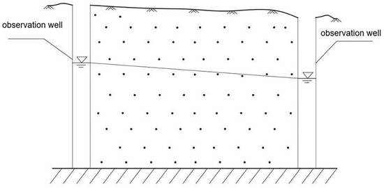
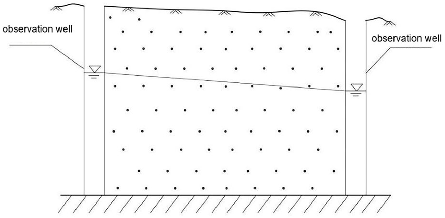
The most classic and widely applied solute transport model under the action of groundwater flow in porous media (as depicted in Figure 1) is a transport model in which a tracer of constant concentration is continuously injected into a semi-infinite sand column (i.e., without consideration of adsorption, decay, etc.). This is the most fundamental model for studying pollutant transport in aquifers. The following assumptions are made regarding the model conditions.
Figure 1.
Migration diagram of composite pollutants in one-dimensional uniform flow field.
- (1)
- The seepage zone is a homogeneous porous medium with semi-infinite length;
- (2)
- The groundwater flow is a one-dimensional flow that conforms to Darcy’s law, and the seepage velocity is a constant v;
- (3)
- Initial tracer concentration in the seepage zone c(x,0) = 0;
- (4)
- From t = 0, the tracer is continuously injected from the x = 0 end to maintain the tracer at the injection end c(0,t) as a constant c0.
The aforementioned conceptual model is the basic model for the migration of pollutants in porous aquifers. The corresponding mathematical model can be summarized by partial differential equations, as (I) [34]:
where c is the concentration of pollutants (mg/L), D is the hydrodynamic dispersion coefficient of pollutants in the porous medium (m2/d), v is the groundwater seepage velocity (m/d), and x is the distance between the measurement point and pollution source (m).
In practical applications, when parameters such as hydraulic gradient, hydraulic conductivity, and porosity remain relatively stable within an aquifer, a monitoring cross-section can be established along the groundwater flow direction downstream of the contamination source. In this scenario, the contamination situation can be simplified into a sufficiently long “sand column” model, thereby transforming the complex three-dimensional problem into a one-dimensional analysis. Specifically, the hydraulic gradient can be calculated using two stable observation wells located upstream and downstream along the cross-section. By combining pumping test data or empirical values to determine hydraulic conductivity and porosity, the groundwater flow velocity (v) can be obtained. Subsequently, based on hydrogeological conditions, an appropriate hydrodynamic dispersion coefficient (D) can be selected. With these parameters, the expected concentration at any given time (t) and distance (x) from the contamination source can be calculated through model (I), enabling prediction of the temporal and spatial distribution of pollutants in groundwater.
It should be noted that Equation (1) is derived under the condition where there is no chemical reaction or any other factors causing changes in the mass of the solute. When adsorption exists at the interface between the solid phase and the liquid phase, the solute in the liquid phase is attracted by the solid-phase surface and transferred to the solid phase, thereby reducing the concentration of the solute in the liquid phase. At this time, the mass change of the solute caused by the adsorption effect can be treated as a source term, then the mathematical model (I) can be summarized as model (II) [35] by partial differential equations as follows:
where R is the retardation factor (dimensionless).
In porous aquifers, the retardation factor is defined as [36]:
where c is the concentration of liquid-phase pollutants (mg/L), cs is the concentration of solid-phase pollutants (mg/kg), ρ is the density of the porous medium (mg/L), n represents the porosity, which is the moisture content in a saturated aquifer, and ∂cs/∂c is the derivative of the concentration of solid-phase pollutants with respect to the concentration of liquid-phase pollutants. According to Equation (9), R > 1, which means that the adsorption effect will slow down the solute migration progress of the considered component. Therefore, R is called the retardation factor or delay factor.
2.1.2. Adsorption Isotherm Models
At present, most studies have used adsorption isotherms to characterize the adsorption features of pollutants. The adsorption isotherm refers to the fact that, at the same temperature, adsorption reaches surface equilibrium, and the adsorption capacity of the solid phase is correlated with the concentration of pollutants in the liquid phase. The existing adsorption isotherm models are mainly classified into three categories: Henry, Freundlich, and Langmuir models.
- The Henry model
The Henry model is a linear adsorption isotherm model, meaning that the adsorption capacity of the solid phase has a linear relationship with the concentration of liquid-phase pollutants, which can be expressed as [37]:
where K1 is the distribution coefficient.
- The Freundlich model
The Freundlich model is a nonlinear adsorption isotherm model, which can be expressed as [37]:
where K2 is the Freundlich coefficient and n is a constant.
- The Langmuir model
The Langmuir model is based on the fact that the adsorption sites on a solid surface are limited, and the adsorption capacity no longer increases when it reaches a limited value. This can be expressed as [38]:
where α is the Langmuir coefficient, and β is the maximum adsorption capacity per unit mass of adsorbate (mg/kg).
These three models can achieve satisfactory results in describing the adsorption phenomenon in the transport process of composite pollutants, which are essentially empirical and subject to specific applicability.
2.2. Machine Learning Methods
2.2.1. Data Sources and Processing
Based on data analyses, we conducted machine learning to study the universally applicable relationship between the adsorption capacity of solid phase cs and the concentration of liquid-phase pollutants c, and calculated the adsorption kinetics parameters. The data sources of machine learning were literature data published in the Web of Science and China National Knowledge Infrastructure databases from 2014 to 2024.
The collected data were combined into three groups. The first group consisted of adsorption test data for heavy metal composite pollutants, and the second group consisted of test data for organic composite pollutants. The number of datasets varied depending on the different test data collected. The third group was formed by combining the data from the first and second groups. The dataset for the heavy metal composite pollutant adsorption test contained 183 sets of data. The types of heavy metals mainly included iron, manganese, and other heavy metal test data, such as cadmium. The dataset for the organic composite pollutant adsorption test consisted of 1148 sets of data, including naphthalene and dichloromethane. During machine learning, 80% of the three groups of data were used as training sets and 20% were used for testing. When training the data, the equilibrium concentration value of liquid-phase pollutants c was taken as the horizontal coordinate, and the equilibrium adsorption capacity of solid-phase pollutants cs was taken as the vertical coordinate.
2.2.2. Model Construction
- RF model
RF is a powerful ensemble classifier based on decision trees [39]. The modelling process mainly includes three steps: first, each decision tree is sampled to generate the training set; second, different decision trees are established for each training subset, and a sufficiently large ‘forest’ is grown using node splitting and random extraction of variables; and third, voting execution is conducted through a large number of decision trees formed by using algorithms.
The hyperparameters of this model were fixed as follows: 500 decision trees, a maximum depth of seven for each tree, and the maximum number of features considered during node splitting is one-third of the total number of features, ensuring that at least one feature was used for node partitioning.
- SVM model
SVM is a supervised machine learning technique based on the structural risk minimization principle and statistical learning theory [39]. According to the linear separability of training samples, SVM can be divided into three learning methods: the hard interval is maximized when linearly separable, soft interval maximization is adopted when approaching linear separability, and kernel function techniques and soft interval maximization are employed when the samples are linearly inseparable.
The model consisted of an input layer, a kernel function mapping layer and an output layer. The samples were mapped to a high-dimensional feature space through the radial basis kernel function. The penalty coefficient was set to 1.0, the kernel function parameter was set to 1/p (where p denotes the total number of features), and the soft interval tolerance was set to 0.0001.
- BPNN model
BPNN is based on cognitive and neuropsychology. It adopts nonlinear continuous transformation functions and constructs a multilayer perceptron model through error backpropagation learning [40]. First, sample data are selected to initialize weights and thresholds, then a neural network model is established, mathematical software is used to train the model to fit the ideal model, and finally, the model is utilized for prediction.
This model was composed of three layers of network structure, namely the input layer, the hidden layer and the output layer. The number of nodes in each layer was c, 10, and cs, respectively. The learning rate was 0.001, the number of iterations was 100, and the error threshold was set to 0.0001. The training utilized multi-layer perceptron to simulate complex nonlinear relationships, minimizing the prediction errors through the gradient descent algorithm to optimize the model parameters.
- DT model
DT is a tree-like structural model composed of nodes and branches. The principle is to learn the classifier using the given samples and complete the classification task using supervised learning [41]. The decision tree algorithm consists of two processes: establishing a model and applying the model for classification. When establishing the model, starting from the root node, the attributes of the sample set are tested, the sub-training set is split, and the cycle continues until the termination condition is met to form a leaf node. When applying the model, the data of the unknown categories were input into the decision tree, and the categories were determined according to the classification rules.
This model was built with the CART algorithm, using the minimum Gini coefficient as the splitting rule and a maximal depth of seven. Its architecture comprised a root node, internal nodes and leaf nodes: the root and internal nodes encoded feature-based decision rules, whereas the leaves stored the predicted values. By recursively splitting the sample set, the sample categories of each sub-node were made as pure as possible, achieving the mapping from features to the target variable.
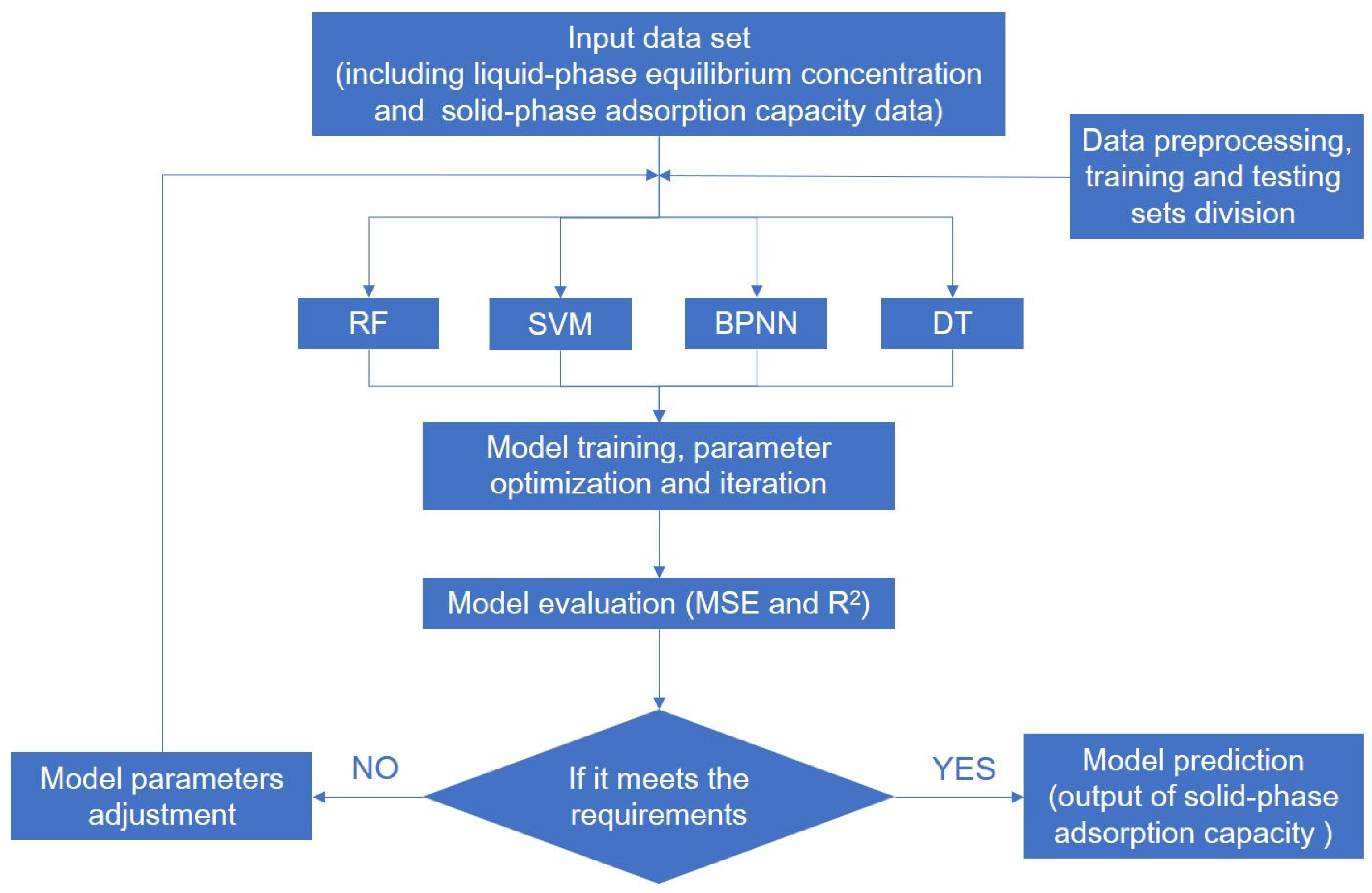
The flowchart of machine learning can be seen in Figure 2.
Figure 2.
Flowchart of machine learning.
2.2.3. Model Evaluation
In this study, two performance evaluation metrics, that is, mean square error (MSE) and the coefficient of determination (R2), are used to assess the performance of each model. The metrics are root and are defined as follows [42]:
where Y is the observed value, is the predicted value, is the mean of the observed value, and n is the number of samples.
3. Results
3.1. Simulation Results of Machine Learning Models
The RF, SVM, BPNN, and DT machine learning models were trained using the three collected datasets, namely heavy metal composite pollutants, organic composite pollutants, and heavy metal and organic combined composite pollutants. The adsorption isotherms obtained, which describe the relationship between the solid-phase adsorption capacity and liquid-phase equilibrium concentration of the test sets are presented below.
3.1.1. Simulation Results of Heavy Metal Composite Pollutants
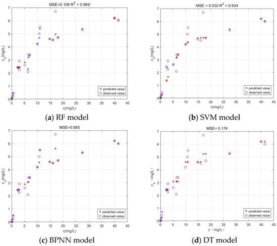
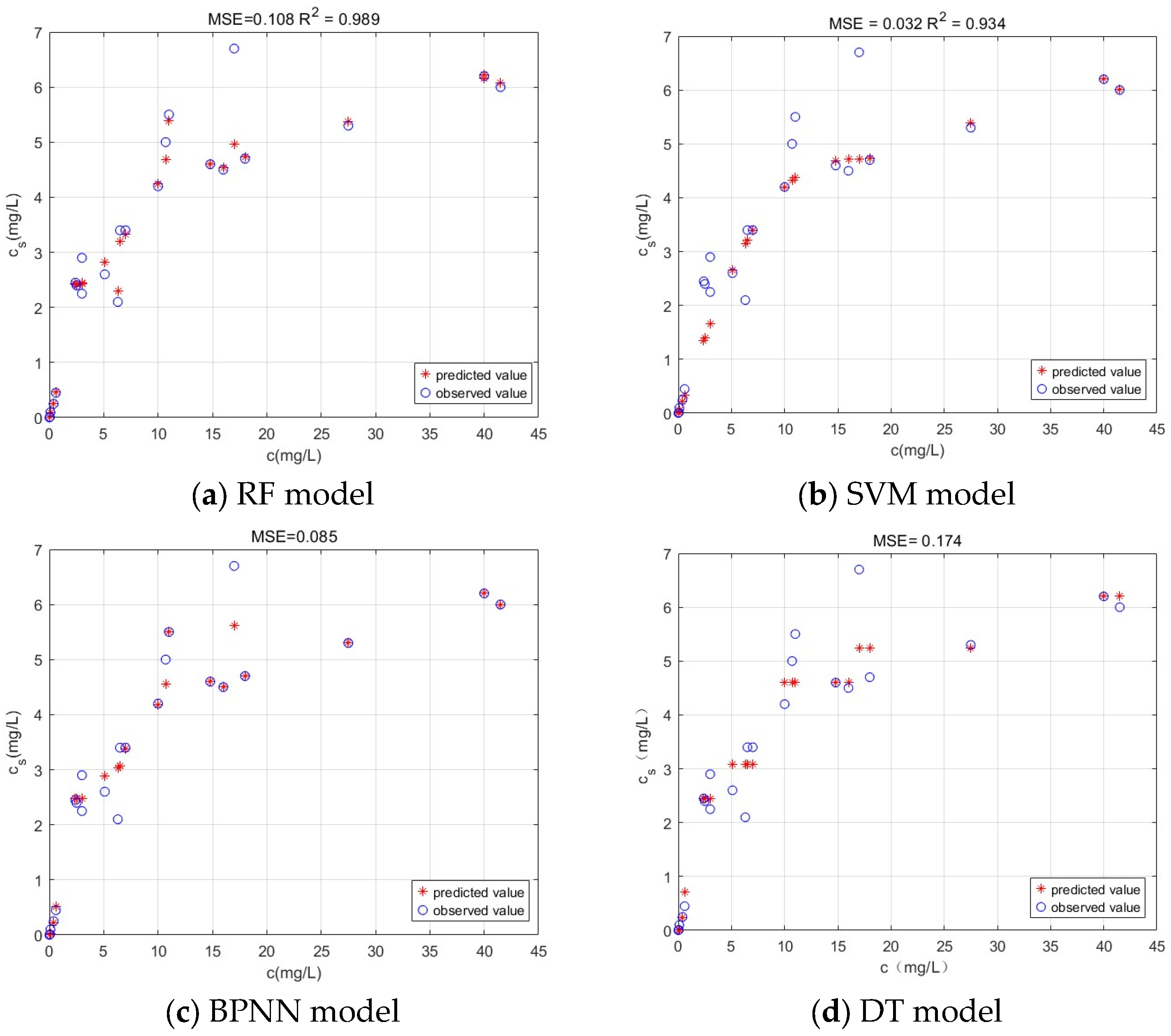
The simulation results for heavy metal composite pollutants trained by the four models are presented in Figure 3.
Figure 3.
Comparison results of heavy metal composite pollutants.
Figure 3 indicates that the respective mean square errors (MSEs) were 0.108, 0.032, 0.085 and 0.174. The RF and SVM models yielded determination coefficients of 0.989 and 0.934.
3.1.2. Simulation Results of Organic Composite Pollutants
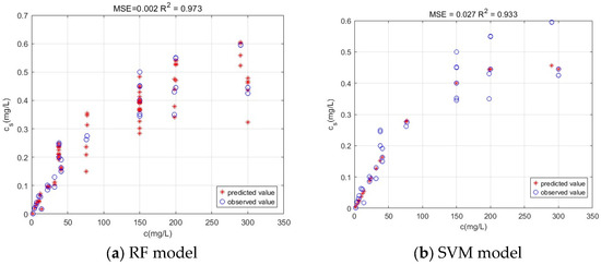
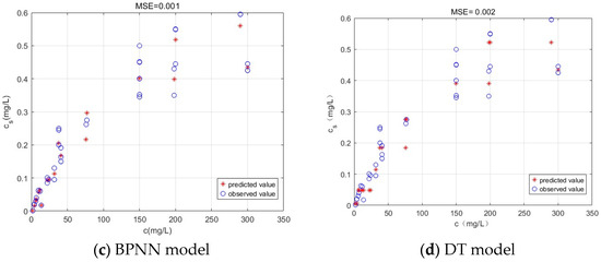
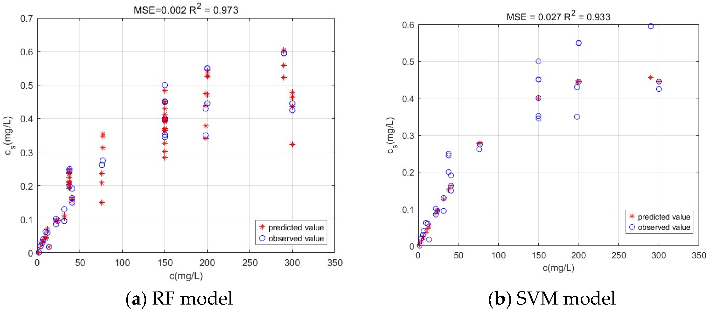
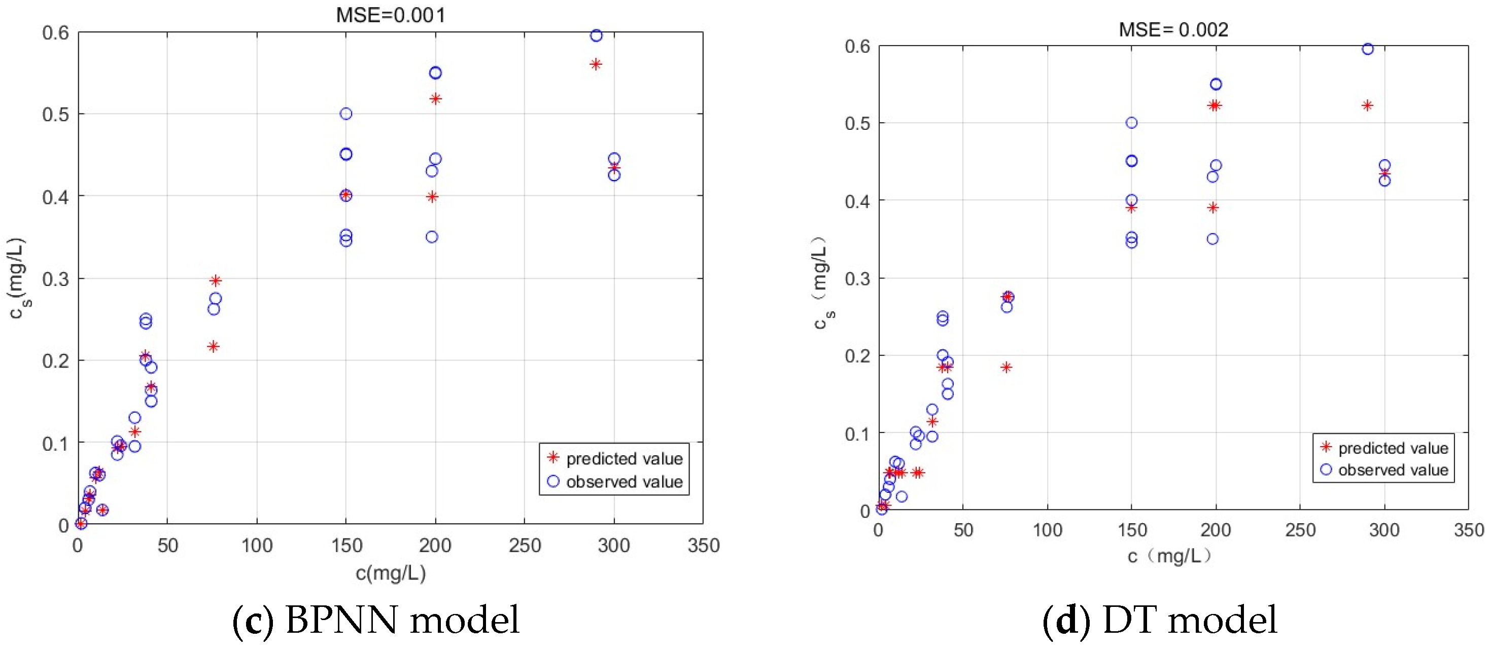
The simulation results of organic composite pollutants are shown in Figure 4.
Figure 4.
Comparison results of organic composite pollutants.
As is seen in Figure 4, the MSEs of the four models were 0.002, 0.027, 0.001 and 0.002, respectively. The RF and SVM models achieved determination coefficients of 0.973 and 0.933, respectively.
3.1.3. Simulation Results of Heavy Metal and Organic Combined Composite Pollutants
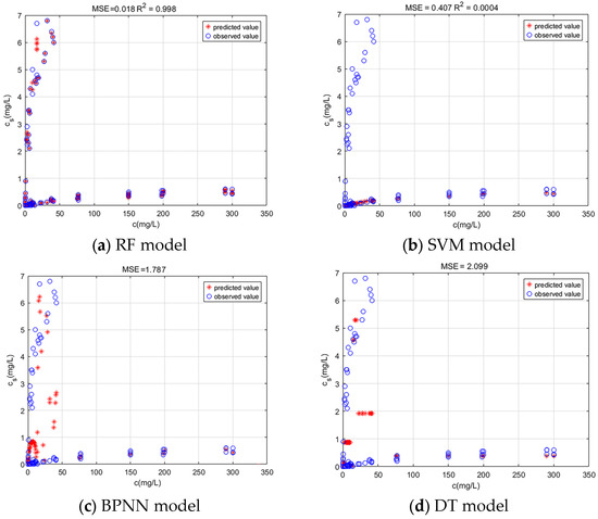
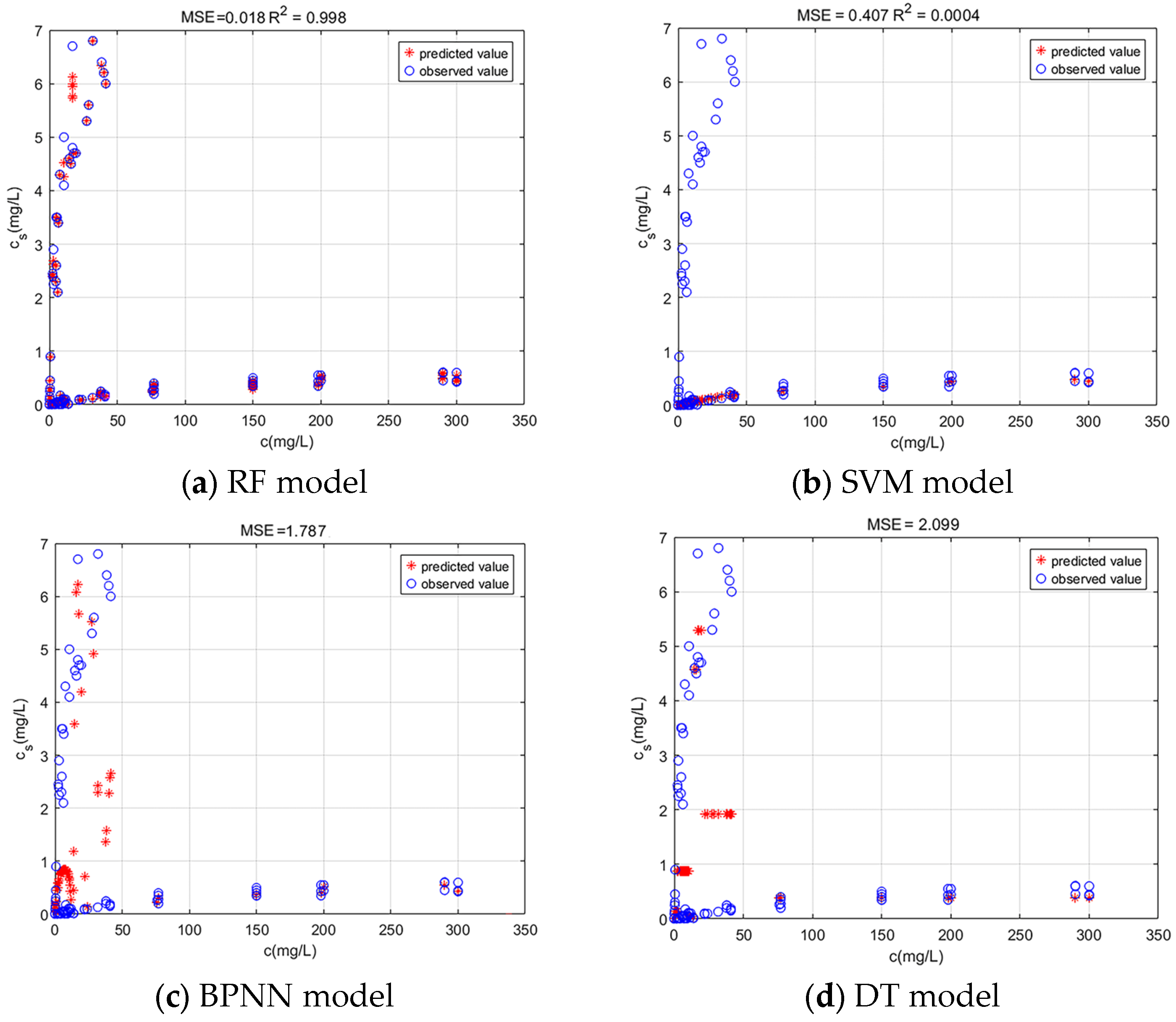
Figure 5 summarizes the training results for the test set that combines heavy metal and organic composite pollutants. The MSEs achieved by the four models were 0.018, 0.407, 1.787 and 2.099, respectively. The RF and SVM models yielded determination coefficients of 0.998 and 0.0004.
Figure 5.
Comparison results of heavy metal and organic combined composite pollutants.
It should be emphasized that the four models yielded markedly divergent results. This disparity stems from the intricate interactions that govern the simultaneous sorption of heavy metals and organic composite pollutants. The calibration data set merges two chemically distinct pollutant classes, so the resulting feature space is heterogeneous, partially overlapping, and class-imbalanced. These contrasting sorption mechanisms therefore raise the learning difficulty for all algorithms. Among them, the SVM model is sensitive to the balance of data distribution and noise. The heterogeneity of the mixed data set makes it difficult for the kernel function to effectively map the optimal separation hyperplane, thereby resulting in large prediction errors. The BPNN model has high requirements for the amount and quality of data. The complex adsorption mechanism of mixed pollutants exceeds the fitting ability of a simple 3-layer network, and it is prone to overfitting or underfitting. The single tree structure of the DT model has weak generalization ability and is unable to capture the complex nonlinear relationships of the mixed data set. It is also susceptible to outliers, resulting in large errors. The RF model, through the ensemble learning of multiple decision trees, can effectively reduce the sensitivity of a single model to the heterogeneity of the data. By randomly sampling and randomly selecting features to cover the adsorption characteristics of both pollutants, it thus exhibits better stability and prediction accuracy on mixed data sets.
3.2. Adsorption Characteristic Analysis
3.2.1. Analysis for Heavy Metal Composite Pollutants and Organic Composite Pollutants
The comparison of MSEs predicted by above four models is shown in Table 1.
Table 1.
Comparison results of MSEs of test sets predicted by four models.
Table 1 shows that for heavy-metal composite pollutants, the SVM model performed best, yielding the lowest MSE of 0.032. For organic composite pollutants, the BPNN model achieved the best accuracy, with an MSE of 0.001. Both values were below 4%, effectively eliminating the random experimental uncertainty.
The nonlinear relationship between the solid-phase adsorption capacity and the liquid-phase equilibrium concentration predicted by machine learning methods is only the relationship between one input quantity and one output quantity, which resolves the influence of different experimental settings, such as pH value, temperature and flow rate, while remaining straightforward to implement.
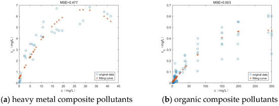
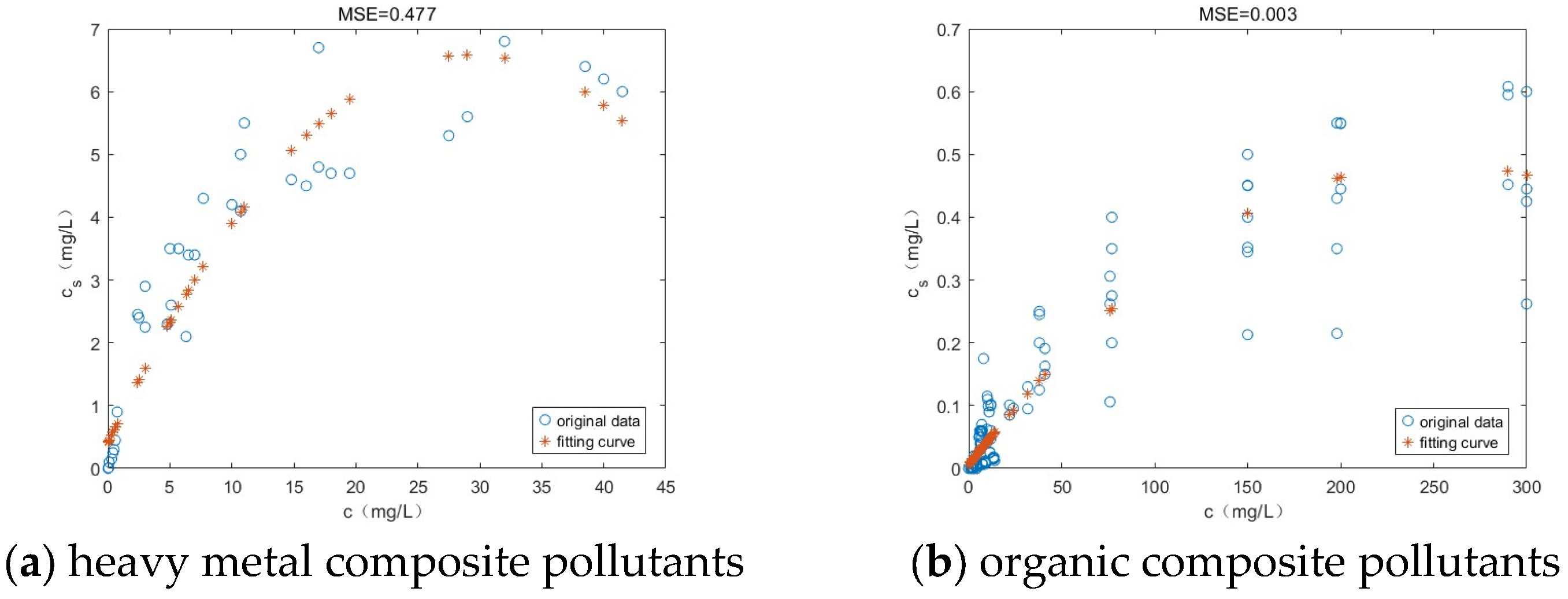
Based on the above analysis, the nonlinear relationship between the solid-phase adsorption capacity and the liquid-phase equilibrium concentration of composite pollutants can be fitted through the unary quadratic function, as presented in Figure 6.
Figure 6.
The fitted adsorption isotherms of composite pollutants.
Figure 6 shows that the adsorption isotherms for both heavy-metal and organic composite pollutants are well described by the Freundlich model, in agreement with numerous experimental studies. From the perspective of data distribution, the liquid-phase equilibrium concentrations of heavy metal pollutants tend to be concentrated between 0 and 2 mg/L, and the dispersion of the data is relatively high when concentrations are above 20 mg/L. For organic pollutants, the equilibrium concentrations are concentrated between 0 and 20 mg/L and tend to be dispersed when they are above 200 mg/L. It should be noted that the experimental data in the database were mostly obtained at low concentrations, where the adsorption characteristics of the two composite pollutants are consistent.
However, at different liquid-phase concentrations, the adsorption isotherms of the two composite pollutants show significant differences. Compared with organic composite pollutants, heavy metal composite pollutants have a higher solid-phase adsorption capacity, and they exhibit a high solid-phase adsorption capacity reaction at low liquid-phase concentrations.
3.2.2. Analysis for Heavy Metal and Organic Combined Composite Pollutants
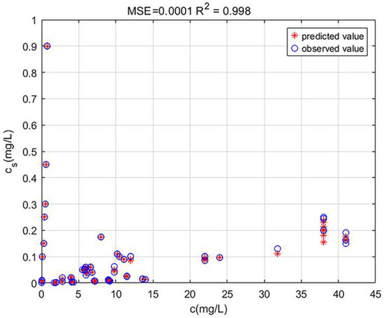
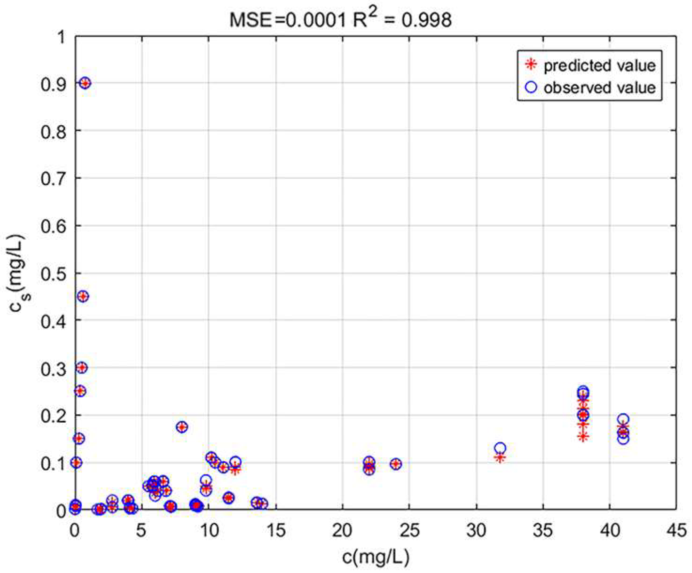
According to Figure 5, for heavy metal and organic combined composite pollutants, the adsorption isotherm obtained through the RF model had the best predictive effect, with an MSE of 0.018. Therefore, the retardation factor of the combined composite pollutants could be estimated using this learned model. For liquid-phase concentrations below 45 mg/L, where data are densely distributed, the RF model was reapplied as displayed in Figure 7.
Figure 7.
Prediction results of heavy metal and organic combined composite pollutants by RF model when c < 45 mg·L−1.
Figure 7 shows an MSE of 0.0001 and a determination coefficient of 0.998, indicating that the RF model predicts well when the concentration is below 45 mg/L.
3.3. Retardation Factor Calculation Examples
In this study, machine learning models were applied to estimate values of cs instead of isotherm models, thereby completing the calculation of retardation factor. This is because isothermal models depend on limited experimental data for parameter fitting and are only capable of characterizing the univariate correlation between adsorption capacity and solute concentration. However, it fails to quantify the combined influence of pH, temperature, soil properties, and other factors that mutually interact during the actual adsorption process of composite pollutants. In contrast, machine-learning models can inherently accommodate the intricate adsorption mechanisms of multi-component contaminants by integrating extensive monitoring data that span diverse experimental conditions. These algorithms autonomously learn the complex, non-linear mappings between competitive adsorption or cooperative adsorption processes and the resulting uptake capacity, thereby eliminating the conditional constraints of single-factor experiments. Consequently, they deliver prediction accuracies that substantially exceed those of traditional isotherm fittings while markedly accelerating parameter acquisition. For instance, the RF model can simultaneously adapt to the distinct adsorption behaviours of heavy metals and organic pollutants, enabling precise parameter prediction for composite pollutants, whereas individual isotherm models are fundamentally unable to achieve this.
3.3.1. Calculation Example for Heavy Metal Composite Pollutants
In the porous aquifer, we assumed that the measured mixed concentration of iron and manganese ions, c, was 5.20 mg/L, the soil density was 1.2 g/cm3 and the porosity was 40%. According to Figure 3b, the predicted value of cs was 2.86 mg/g. With Equation (9), the retardation factor for heavy metal composite pollutants is 5.45.
3.3.2. Calculation Example for Organic Composite Pollutants
For composite pollutants of naphthalene and dichloromethane, we again set c = 5.20 mg/L and kept the same porous medium conditions as in Section 3.3.1. Figure 4c gives cs = 0.02 mg/g, so Equation (9) yields a retardation factor of 780 for organic composite pollutants.
3.3.3. Calculation Example for Heavy Metal and Organic Combined Composite Pollutants
For combined composite pollutants of iron ions and dichloromethane, we set c = 5.20 mg/L and used the same porous medium conditions as in Section 3.3.1. Figure 7 gives cs = 0.03 mg/g, so Equation (9) gives a retardation factor of 520 for the combined pollutants.
The examples above demonstrate that machine learning models can reliably predict the solid-phase adsorption capacity of composite pollutants and obtain corresponding retardation factors. When the liquid-phase equilibrium concentration is identical, the predicted value of the retardation factor of heavy metal and organic composite pollutants is closer to that of organic composite pollutants. This might be because the training set is dominated by organic composite pollutants: the number of them is more than threefold that of heavy metal composite pollutants. Consequently, the data training results of heavy metal and organic combined composite pollutants are more consistent with the adsorption laws of organic composite pollutants.
In addition, the analysis in Section 3.2 and the calculation examples show that, despite their similar characteristics, organic composite pollutants have much higher retardation factors than heavy metal composites. Therefore, when the accuracy of the analytical techniques is sufficient, the retardation factors for these two types of pollutants should be calculated separately.
4. Discussion
This study systematically compared the applicability of four models for three types of composite pollutants, expanding the application scenarios of machine learning in the research of adsorption of pollutants. The predicted MSEs of the optimal model were all lower than 4%, indicating that the machine learning models can achieve high-precision adsorption quantity predictions. The retardation factor of organic composite pollutants is 143 times that of heavy metal composite pollutants, suggesting that the migration rate of organic pollutants in the pore aquifers is much lower than that of heavy metal pollutants, providing a quantitative basis for the prioritization of pollution control. When the liquid-phase concentration is lower than 45 mg/L, the predicted MSE of the RF model for heavy metal and organic combined composite pollutants reaches to 0.0001, and the determination coefficient reaches 0.998, indicating that in the low-concentration range, the model prediction accuracy is higher and its applicability is stronger. By integrating a large amount of literature data, the randomness errors of a single experiment were effectively eliminated, and no complex experimental equipment was required, significantly reducing the parameter acquisition cost, which is consistent with the viewpoint proposed by Dahal et al. [18].
However, all data used in this study were extracted from published literature, and some of them did not report experimental conditions in detail, potentially compromising the comprehensiveness of model training. The data collected contained far fewer heavy metal composite pollutants than organic composite pollutants data, so the training process is biased toward the sorption characteristics of organic pollutants and may degrade the balance of predictions for composite contaminants. In addition, the developed models use only liquid-phase concentration as an input feature and ignore other key factors that govern sorption, such as pH, temperature, and porosity, thereby limiting their range of applicability. Furthermore, the predicted results and the calculated retardation factors have not been directly validated against column experiments or field-scale monitoring data, so the reliability of the models under real-world conditions remains to be demonstrated.
5. Conclusions
This study analyzed the adsorption characteristics of various types of composite pollutants based on four commonly used machine learning models. The results revealed that for heavy metal composite pollutants, organic composite pollutants, and heavy metal and organic combined composite pollutants, the SVM, BPNN, and RF models predicted the adsorption isotherms with the greatest effect, respectively. The adsorption isotherms of both heavy metal and organic composite pollutants conform to the Freundlich model, with data for these two composite pollutants being more concentrated at low concentrations and scattered at high concentrations. Heavy metal composite pollutants exhibit a higher solid-phase adsorption capacity than organic composites, particularly at low liquid-phase concentrations, and they undergo a reaction with a high solid-phase adsorption capacity. Moreover, calculation examples indicate that organic composite pollutants have much larger retardation factors than heavy metal composites, and that at the same liquid-phase equilibrium concentration, the predicted retardation factor for heavy metal and organic combined composite pollutants is closer to that of the organic composites.
Author Contributions
Conceptualization, L.W.; methodology, L.W. and T.W.; validation, L.W.; formal analysis, L.W. and T.W.; data curation, H.R. and F.L.; visualization, T.W. and H.R.; writing—original draft preparation, L.W.; writing—review and editing, T.W.; supervision, F.L. All authors have read and agreed to the published version of the manuscript.
Funding
This research was funded by the Natural Science Research Project of the Anhui Educational Committee, grant numbers 2022AH040302 and 2024AH050575.
Data Availability Statement
The original contributions presented in this study are included in the article. Further inquiries can be directed to the corresponding author.
Conflicts of Interest
The authors declare no conflicts of interest.
Abbreviations
The following abbreviations are used in this manuscript:
| RF | Random Forest |
| SVM | Support Vector Machine |
| BPNN | Back Propagation Neural Network |
| DT | Decision Tree |
| MSE | Mean Square Error |
References
- Feng, S.; Yu, H. Source apportionment and health risk assessment of heavy metals in groundwater of rural area: A case study in Huaibei plain, China. Hum. Ecol. Risk Assess. 2024, 30, 220–236. [Google Scholar] [CrossRef] [Scilit]
- Huang, S.L.; Li, Q.; Xu, D.S. Heavy metal pollution in Suzhou urban soils and its health risk assessment. Adv. Mater. Res. 2012, 534, 244–248. [Google Scholar] [CrossRef] [Scilit]
- Can, N.; Ömür, B.C.; Altındal, A. Modeling of heavy metal ion adsorption isotherms onto metallophthalocyanine film. Sensor Actuat. B-Chem. 2016, 237, 953–961. [Google Scholar] [CrossRef] [Scilit]
- Yimer, M.; Ansari, S.N.; Berehe, B.A.; Gudimella, K.K.; Gedda, G.; Girma, W.M.; Hasan, N.; Tasneem, S. Adsorptive removal of heavy metals from wastewater using Cobalt-diphenylamine (Co-DPA) complex. BMC Chem. 2024, 18, 23. [Google Scholar] [CrossRef] [Scilit]
- Chen, Y.Y.; Cheng, X.T.; Zeng, Y.Q. The occurrence of microplastic in aquatic environment and toxic effects for organisms. Int. J. Environ. Sci. Technol. 2023, 20, 10477–10490. [Google Scholar] [CrossRef] [Scilit]
- Ahmed, D.N.; Ibrahim, M.O.; Abdul-Kareem, M.B.; Shoshan, A.A.A.; Faisal, A.A.H. Novel low-cost composite sorbent for remediating synthetic sanitary landfill leachates: Batch and column study. Alex. Eng. J. 2023, 64, 205–218. [Google Scholar] [CrossRef] [Scilit]
- Akortia, E.; Okonkwo, J.O. Transport and retention of polybrominated diphenyl ether in landfill and e-waste contaminated soils: A laboratory-scale soil flushing approach. Int. J. Environ. Sci. Technol. 2022, 19, 2867–2876. [Google Scholar] [CrossRef] [Scilit]
- Zhang, J.; Zhang, J.; Xing, B.; Liu, G.; Liang, Y. Study on the effect of municipal solid landfills on groundwater by combining the models of variable leakage rate, leachate concentration, and contaminant solute transport. J. Environ. Manag. 2021, 292, 112815. [Google Scholar] [CrossRef] [Scilit]
- Lu, S.; Jia, C.; Liu, S.; Yang, X. Simulation and prediction of soil contamination migration for organic compounds under multiple scenarios in coastal areas of Rizhao City, Shandong Province. Environ. Monit. Assess. 2025, 197, 1323. [Google Scholar] [CrossRef] [Scilit]
- Xue, S.; Ke, W.; Zeng, J.; Baltazar Tabelin, C.; Xie, Y.; Tang, L.; Xiang, C.; Jiang, J. Pollution prediction for heavy metals in soil-groundwater systems at smelting sites. Chem. Eng. J. 2023, 473, 145499. [Google Scholar] [CrossRef] [Scilit]
- Agboola, O.; Nwankwo, O.J.; Akinyemi, F.A.; Chukwuka, J.C.; Ayeni, A.O.; Popoola, P.; Sadiku, R. Adsorptive removal of Fe and Cd from the textile wastewater using ternary bio-adsorbent: Adsorption, desorption, adsorption isotherms and kinetic studies. Discov. Sustain. 2024, 5, 312. [Google Scholar] [CrossRef] [Scilit]
- Lu, D.; Xia, Y.; Geng, N.; Wang, H.; Qian, J.; Xu, C. Estimation parameters of soil solute transport by using the electric resistivity method. Processes 2022, 10, 975. [Google Scholar] [CrossRef] [Scilit]
- Guo, M.; Wan, J.; Huang, K. Characteristics of solute transport continuously released from coastal unconfined aquifers under the tidal action based on laboratory experiment. J. Earth Sci. 2024, 35, 1738–1748. [Google Scholar] [CrossRef] [Scilit]
- Feng, Y.; Zhou, S.; Wan, J.; Wang, S.; Du, Y.-j. Evalution of hydrodynamic dispersion coefficients of nickel and zinc released from a contaminated clay solidified/stabilized by a low-carbon binder. Chin. J. Geotech. Eng. 2022, 44, 151–154. [Google Scholar] [CrossRef]
- Malekzadeh, M.; Kardar, S.; Shabanlou, S. Simulation of groundwater level using MODFLOW, extreme learning machine and Wavelet-Extreme Learning Machine models. Groundw. Sust. Dev. 2019, 9, 100279. [Google Scholar] [CrossRef] [Scilit]
- EL Osta, M.; Masoud, M.; Niyazi, B.; Al-Amri, N.; Alqarawy, A.; El-baki, M.S.A.; Elsayed, S. Utilizing machine learning algorithms to improve predictions of groundwater quality indices for irrigation in an arid environment of Saudi Arabia. Environ. Earth Sci. 2025, 84, 389. [Google Scholar] [CrossRef] [Scilit]
- Sah, P.K.; Saurav; Singh, S.K.; Kumar, S.S. Assessment of tree-based machine learning models and empirical equations to predict thermal conductivity of bentonite-based backfill material using experimentally measured data. Environ. Earth Sci. 2025, 84, 379. [Google Scholar] [CrossRef] [Scilit]
- Dahal, K.; Sharma, S.; Shakya, A.; Talchabhadel, R.; Adhikari, S.; Pokharel, A.; Sheng, Z.; Pradhan, A.M.S.; Kumar, S. Identification of groundwater potential zones in data-scarce mountainous region using explainable machine learning. J. Hydrol. 2023, 627, 130417. [Google Scholar] [CrossRef] [Scilit]
- Khan, Q.; Liaqat, M.U.; Mohamed, M.M. A comparative assessment of modeling groundwater vulnerability using DRASTIC method from GIS and a novel classification method using machine learning classifiers. Geocarto Int. 2022, 37, 5832–5850. [Google Scholar] [CrossRef] [Scilit]
- He, T.; Chang, H.; Zhang, D. Identification of physical processes and unknown parameters of 3D groundwater contaminant problems via theory-guided U-net. Stoch. Environ. Res. Risk A 2024, 38, 869–900. [Google Scholar] [CrossRef] [Scilit]
- Teimoori, S.; Olya, M.H.; Miller, C.J. Groundwater level monitoring network design with machine learning methods. J. Hydrol. 2023, 625, 130145. [Google Scholar] [CrossRef] [Scilit]
- Yin, J.; Medellín-Azuara, J.; Escriva-Bou, A.; Liu, Z. Bayesian machine learning ensemble approach to quantify model uncertainty in predicting groundwater storage change. Sci. Total Environ. 2021, 769, 144715. [Google Scholar] [CrossRef] [Scilit]
- Liu, J.; Gu, J.; Li, H.; Carlson, K.H. Machine learning and transport simulations for groundwater anomaly detection. J. Comput. Appl. Math. 2020, 380, 112982. [Google Scholar] [CrossRef] [Scilit]
- Mallikarjuna, B.; Sathish, K.; Venkata Krishna, P.; Viswanathan, R. The effective SVM-based binary prediction of ground water table. Evol. Intell. 2021, 14, 779–787. [Google Scholar] [CrossRef] [Scilit]
- Gómez-Escalonilla, V.; Montero-González, E.; Díaz-Alcaide, S.; Martín-Loeches, M.; Del Rosario, M.R.; Martínez-Santos, P. A machine learning approach to site groundwater contamination monitoring wells. Appl. Water Sci. 2024, 14, 250. [Google Scholar] [CrossRef] [Scilit]
- Torres-Martínez, J.A.; Mahlknecht, J.; Kumar, M.; Loge, F.J.; Kaown, D. Advancing groundwater quality predictions: Machine learning challenges and solutions. Sci. Total Environ. 2024, 949, 174973. [Google Scholar] [CrossRef] [Scilit]
- Pandya, H.; Jaiswal, K.; Shah, M. A Comprehensive Review of Machine Learning Algorithms and Its Application in Groundwater Quality Prediction. Arch. Comput. Methods Eng. 2024, 31, 4633–4654. [Google Scholar] [CrossRef] [Scilit]
- Thanh, N.N.; Thunyawatcharakul, P.; Ngu, N.H.; Chotpantarat, S. Global review of groundwater potential models in the last decade: Parameters, model techniques, and validation. J. Hydrol. 2022, 614, 128501. [Google Scholar] [CrossRef] [Scilit]
- Soekarno, I.; Hadihardaja, I.K.; Cahyono, M. A study of hold-out and k-fold cross validation for accuracy of groundwater modeling in tidal lowland reclamation using extreme learning machine. In Proceedings of the 2014 2nd International Conference on Technology, Informatics, Management, Engineering & Environment, Bandung, Indonesia, 19–21 August 2014; pp. 228–233. [Google Scholar]
- Hosseini, F.S.; Choubin, B.; Mako, M.B.G.K. Susceptibility assessment of groundwater nitrate contamination using an ensemble machine learning approach. Groundwater 2023, 61, 510–516. [Google Scholar] [CrossRef] [Scilit]
- Yue, L.; Junjie, W.; Mingwei, L. Numerical model for contaminant preferential migration based on flow net element. Rock Soil Mech. 2015, 36, 3007–3014. [Google Scholar] [CrossRef]
- Guo, L.; Qian, L.; Xu, M.; Zhang, Y.; Kang, X.; Xiao, X.; Zhang, Q. Effect of the loam inter-layer on the migration and breakthrough of benzene under constant flow in the unsaturated zone: Column experiments. Water Sci. Technol. 2019, 79, 207–217. [Google Scholar] [CrossRef] [Scilit]
- Yan, H.; Wu, J.; Thomas, H.R.; Ding, H.; Zhan, L.; Xie, H. Analytical model for coupled consolidation and diffusion of organic contaminant transport in triple landfill liners. Geotext. Geomembr. 2021, 49, 489–499. [Google Scholar] [CrossRef] [Scilit]
- Tu, T.; Ercan, A.; Kavvas, M.L. One-dimensional solute transport in open channel flow from a stochastic systematic perspective. Stoch. Environ. Res. Risk Assess. 2019, 33, 1403–1418. [Google Scholar] [CrossRef] [Scilit]
- Wang, J.; Shao, M. A comparitive analysis of boundary layer methods in solving convection-dispersion equation of solute transport. Acta Pedol. Sin. 2022, 59, 964–974. [Google Scholar] [CrossRef]
- Jia, S.; Ma, F.; Yang, Z.; Zhou, Z.; Ling, H.; Lan, T.; Wang, W.; Tian, Y.; Thanh, H.V.; Soltanian, M.R.; et al. Retardation factor scaling for contaminant transport in fractured media. Adv. Water Resour. 2024, 188, 104709. [Google Scholar] [CrossRef] [Scilit]
- Tran, H.N.; Lima, E.C.; Juang, R.; Bollinger, J.; Chao, H. Thermodynamic parameters of liquid–phase adsorption process calculated from different equilibrium constants related to adsorption isotherms: A comparison study. J. Environ. Chem. Eng. 2021, 9, 106674. [Google Scholar] [CrossRef] [Scilit]
- Wang, J.; Wang, B.; Wen, Z.; Zhao, N.; Li, T.; Zhao, W. Adsorption process optimization and adsorbent evaluation based on langmuir isotherm model. Langmuir 2023, 39, 16404–16414. [Google Scholar] [CrossRef] [Scilit]
- Naghibi, S.A.; Ahmadi, K.; Daneshi, A. Application of Support Vector Machine, Random Forest, and Genetic Algorithm Optimized Random Forest Models in Groundwater Potential Mapping. Water Resour. Manag. 2017, 31, 2761–2775. [Google Scholar] [CrossRef] [Scilit]
- Wang, G.; Wang, J.; Wang, J.; Yu, H.; Sui, Y. Study on Prediction Model of Soil Nutrient Content Based on Optimized BP Neural Network Model. Commun. Soil. Sci. Plan. 2023, 54, 463–471. [Google Scholar] [CrossRef] [Scilit]
- Li, F.; Zhang, X.; Ji, Y. Decision tree model to classify wastewater evaporation. Ind. Eng. Chem. Res. 2023, 62, 8111–8117. [Google Scholar] [CrossRef] [Scilit]
- Pence, I.; Yıldırım, R.; Siseci Cesmeli, M.; Güngör, A.; Akyüz, A. Evaluation of machine learning approaches for estimating thermodynamic properties of new generation refrigerant R513A. Sustain. Energy Technol. Assess. 2023, 55, 102973. [Google Scholar] [CrossRef] [Scilit]

Disclaimer/Publisher’s Note: The statements, opinions and data contained in all publications are solely those of the individual author(s) and contributor(s) and not of MDPI and/or the editor(s). MDPI and/or the editor(s) disclaim responsibility for any injury to people or property resulting from any ideas, methods, instructions or products referred to in the content. |
© 2026 by the authors. Licensee MDPI, Basel, Switzerland. This article is an open access article distributed under the terms and conditions of the Creative Commons Attribution (CC BY) license.