


Abstract
Multi-reservoir joint operation is a high-dimensional, nonlinear, multi-input multi-output (MIMO) water-allocation problem. This study aimed to map the state variables of multiple water sources directly to the water allocated to each user with a single end-to-end model. A model combining a one-dimensional convolutional neural network (CNN), a bidirectional long short-term memory network (BiLSTM) and the Sparrow Search Algorithm (SSA) was developed: the CNN extracted local coupling features along an ordered source–user feature vector, the BiLSTM captured temporal dependencies within a historical window, and the SSA jointly tuned the hidden-unit number, the initial learning rate and the L2 coefficient. The model was applied to monthly operation records of the Hongze Lake–Luoma Lake–Yangtze Diversion system in the Eastern Route of China’s South-to-North Water Diversion Project. On the held-out test period, the model attained an average R2 of 0.8637 and an average MAPE of 20.61%; the per-output test R2 values were 0.9403 (Hongze Lake supply), 0.8114 (Luoma Lake supply) and 0.8393 (Yangtze diversion supply). Relative to a plain BiLSTM, the full model raised R2 from 0.7763 to 0.8637 and reduced RMSE by 21.9%. Predictability differed among the three outputs, and the Luoma Lake output showed mild overfitting; a two-stage physical-constraint correction kept the allocations within the available-supply bound. The model provides a quantitative data-driven reference for multi-source water-allocation analysis and is intended as the mapping-simulation component of a closed-loop scheduling framework to be developed in future work, rather than as a stand-alone operational decision maker.
1. Introduction
Water resources are fundamental natural assets and strategic economic resources supporting human survival and socioeconomic development. Against the backdrop of intensifying global climate change and rapid urbanization, the uneven spatiotemporal distribution of water resources and growing supply–demand mismatches have become increasingly prominent worldwide. In China, the completion of cascade hydropower bases across major river basins has substantially reshaped the hydrological regime and spatiotemporal pattern of streamflow. Fundamentally, multi-reservoir joint operation is a high-dimensional complex system that governs the spatiotemporal allocation of water across multiple sources and users. Operation decisions are governed by a suite of interdependent variables—reservoir inflow, outflow, storage state, dynamic user demand and allocation priorities—intertwined with strong nonlinear couplings. This makes multi-reservoir joint operation a typical MIMO complex mapping problem. Traditional rule-based operation charts, while widely adopted in practice, only serve as a reference and exhibit limited adaptability to complex, evolving hydrological conditions [1]. Data-driven methods based on artificial neural networks, support vector regression, decision trees and ensemble learning [2,3,4] can mine implicit operational patterns from historical records to a certain extent. However, their relatively simple network structures fail to fully capture the complex couplings among multiple water sources and users. Feature engineering relies heavily on expert domain knowledge, leading to insufficient generalization and degraded accuracy when applied to MIMO operation scenarios [5].
In recent years, deep learning has demonstrated considerable potential in reservoir operation and hydrological forecasting due to its superior nonlinear fitting capacity and end-to-end learning capability. For temporal sequence modeling, long short-term memory (LSTM) networks, with their unique gating mechanism, effectively capture long-range temporal dependencies in hydrological time series and have become a mainstream modeling tool in this field. Kratzert et al. [6] first applied LSTM to rainfall–runoff modeling across 241 catchments. They reported significant performance improvements over traditional lumped hydrological models, and established a new paradigm for deep learning-based hydrological modeling. Zhang et al. [7] coupled complete ensemble empirical mode decomposition with adaptive noise (CEEMDAN) with LSTM for urban reservoir water quality prediction, achieving prediction errors below 10% for total nitrogen, ammonia nitrogen, total phosphorus and pH.
Regarding CNN-LSTM hybrid architectures, Fang et al. [8] proposed a Conv-LSTM framework for extracting operation rules of cascade reservoirs in the Yalong River basin. The framework captures the spatiotemporal distribution of areal precipitation. The LSTM module aggregates precipitation features and historical reservoir operation information, achieving Nash–Sutcliffe Efficiency (NSE) above 0.95 and average relative error below 10% for all reservoirs. This verified the advantages of the CNN-LSTM architecture for multi-reservoir operation rule extraction.
For signal decomposition-integrated deep learning methods, Xu et al. [9] proposed a CEEMDAN-VMD-CABES-LSTM hybrid monthly runoff prediction model. It adopts a secondary decomposition strategy to decouple multi-scale frequency and trend components of runoff series. Compared with a single LSTM model, RMSE decreased by 71.09% and 65.13% at the Xiajiang and Yingluoxia hydrological stations, respectively, with NSE approaching 1.0. Zhang et al. [10] developed a CEEMDAN-SSA-BiLSTM daily runoff prediction model. In this model, the Sparrow Search Algorithm (SSA) is used to optimize BiLSTM hyperparameters. The model achieved NSE values of 0.95–0.97 at four hydrological stations along the Yellow River. This confirms the effectiveness of the “decomposition–prediction–reconstruction” paradigm combined with bidirectional temporal modeling for multi-step runoff forecasting.
Regarding automatic hyperparameter optimization, Wang et al. [11] systematically evaluated five hyperparameter optimization techniques for neural network-based surface water quality prediction. The results showed that Bayesian optimization based on the tree-structured Parzen estimator achieved the most stable convergence, most reasonable search direction and highest hyperparameter consistency. It was recommended as the preferred method for deep learning hyperparameter tuning in water resources research. Tran et al. [12] applied Bayesian optimization to simultaneously select input predictors and tune deep learning hyperparameters. They constructed an LSTM-GRU-BiLSTM reservoir outflow prediction model, and demonstrated the dual value of Bayesian optimization in variable screening and structural tuning. Proposed by Xue and Shen [13] in 2020, the Sparrow Search Algorithm (SSA) is a swarm intelligence optimization algorithm. It is inspired by the foraging and anti-predation behaviors of sparrow flocks. Tested on 19 benchmark functions, it outperformed the Grey Wolf Optimizer (GWO), Particle Swarm Optimization (PSO) and Gravitational Search Algorithm (GSA) in terms of solution accuracy, convergence speed and robustness. It provides a new swarm intelligence tool for deep learning hyperparameter optimization.
Regarding attention mechanisms and spatiotemporal feature enhancement, Li et al. [14] developed a CNN-BiLSTM-Attention hybrid model for surface water quality prediction. It integrates an attention mechanism under an encoder–decoder framework to adaptively weight key spatiotemporal features. The model outperformed CNN-LSTM and single LSTM models in both prediction accuracy and stability. Zhang et al. [15] compared the performance of spatial attention (SAM), temporal attention (TAM) and dual attention mechanisms coupled with CNN-LSTM. The results showed that the dual attention model achieved an NSE of 0.967 for dissolved oxygen prediction, an 18.4% improvement over the baseline CNN-LSTM. Wu et al. [16] proposed a Transformer-based deep reinforcement learning method for multi-reservoir multi-objective operation. It uses multi-head self-attention to capture complex reservoir–user spatial correlations. In a case study of the Colorado River basin (Lake Mead and Lake Powell), power generation increased by 10.11% and ecological flow deviation decreased by 39.69%, highlighting the great potential of Transformer-based architectures in reservoir operation. Regarding intelligent operation rule extraction, Qi et al. [17] combined a Combinatorial Evolution Network (CEN) with differential evolution to automatically extract implicit cascade reservoir operation rules via joint feature–hyperparameter optimization. It reduced discharge simulation RMSE by 5.98–60.98% compared with traditional benchmark models. This work provided a new methodological reference for data-driven intelligent operation rule derivation.
Nevertheless, existing research has several notable limitations. First, most studies target single-reservoir or single-objective operation, with limited MIMO mapping research for multi-source multi-user systems. Such approaches fail to characterize the many-to-many coupling relationships inherent in multi-reservoir joint water supply. Ma et al. [18] developed an MIMO operation rule learning model for cascade hydropower systems. The results showed that MIMO systematically reduced RMSE by approximately 20% and increased annual power generation by 1.2% compared with multi-input single-output (MISO) models. This reveals the advantage of joint modeling for capturing reservoir synergy effects. However, that work focused exclusively on power generation; its input–output structure does not account for the complex spatiotemporal matching between multiple water sources and users in water supply allocation. To date, MIMO mapping for multi-source multi-user water distribution remains an underexplored research gap. Second, existing research emphasizes temporal dependency extraction but lacks explicit modeling of local source–user coupling features induced by the physically ordered feature vector such as upstream–downstream hydraulic connections and inter-user water competition. Graph neural networks and spatiotemporal attention mechanisms have recently been applied to capture spatial dependencies among reservoirs. For example, Fan et al. [19] used an adaptive graph attention network to dynamically capture hydrological connectivity among reservoirs. The method was validated in runoff forecasting for 30 reservoirs in the Colorado River basin. However, such works target runoff prediction or flood control; their spatial modeling is limited to inter-reservoir hydraulic relationships and does not explicitly treat the source–user water supply network topology as a modeling object. Third, hyperparameter tuning mostly relies on manual experience or simple grid search; swarm-intelligence-based joint optimization of all key CNN-BiLSTM hyperparameters has not been fully investigated in the reservoir operation domain. SSA-optimized CNN-BiLSTM has shown promising performance in other time-series prediction fields such as gas concentration prediction [20] and groundwater level forecasting. It enables joint global optimization of CNN kernel size/filter number, BiLSTM hidden units, attention weights and learning rate, improving prediction accuracy by over 20% compared with traditional models. Yet this joint optimization strategy has not been applied to MIMO reservoir operation mapping, and the global joint optimization of multiple heterogeneous hyperparameters remains an unresolved challenge. Fourth, the “decomposition–prediction–reconstruction” paradigm performs well in single-variable runoff forecasting, but its applicability to MIMO multivariate coupled systems requires verification. Zhao et al. [21] proposed a CEEMDAN-SVMD secondary decomposition BiLSTM model. It uses sample entropy to identify high-frequency intrinsic mode functions (IMFs), improving NSE by 6.5–17.9% and R2 by 4.0–9.3% compared with single models. However, it remains limited to single-station runoff series and has not been extended to MIMO multivariate coupling scenarios. In addition, physics-informed embedding is another important pathway to improve model interpretability. Yu et al. [22] proposed physics-encoded LSTM (P-LSTM). It embeds basin water balance and reservoir physical constraints directly into the network structure. It achieved tightly coupled physical consistency in cascade reservoirs of the Han River basin, lifting storage simulation NSE from negative values to 0.50–0.80. Signal decomposition and physics encoding enhance model performance from two complementary dimensions—multi-scale feature decoupling and physical consistency—but their synergistic mechanism in MIMO scenarios has not been established.
To address the above limitations, this paper proposes an SSA-CNN-BiLSTM MIMO mapping model for multi-reservoir joint operation. Taking multi-source state variables and multi-user demand features as inputs and optimized water allocation discharges as outputs, it constructs an end-to-end mapping relationship: a one-dimensional CNN extracts local source–user coupling features induced by the physically ordered feature vector of the water supply network along the source–user dimension, while BiLSTM bidirectionally captures temporal dependencies of the inflow–demand process. The SSA performs global joint auto-optimization of all key CNN-BiLSTM hyperparameters. The theoretical contribution of this study is extending the SSA-CNN-BiLSTM architecture to MIMO mapping for multi-source multi-user reservoir operation, filling research gaps in spatial coupling feature extraction and swarm-intelligence joint hyperparameter optimization. From a practical perspective, the model can be further coupled with evolutionary algorithms such as genetic algorithms [23] to form an integrated “state perception–mapping simulation–optimal decision” framework, providing a quantitative reference for scheduling analysis for unified basin water resources management. Beyond the studied system, the proposed MIMO mapping provides a transferable data-driven paradigm for multi-source, multi-user water supply systems in general, where heterogeneous sources, competing users and constrained conveyance routes must be represented jointly.
2. Study Area
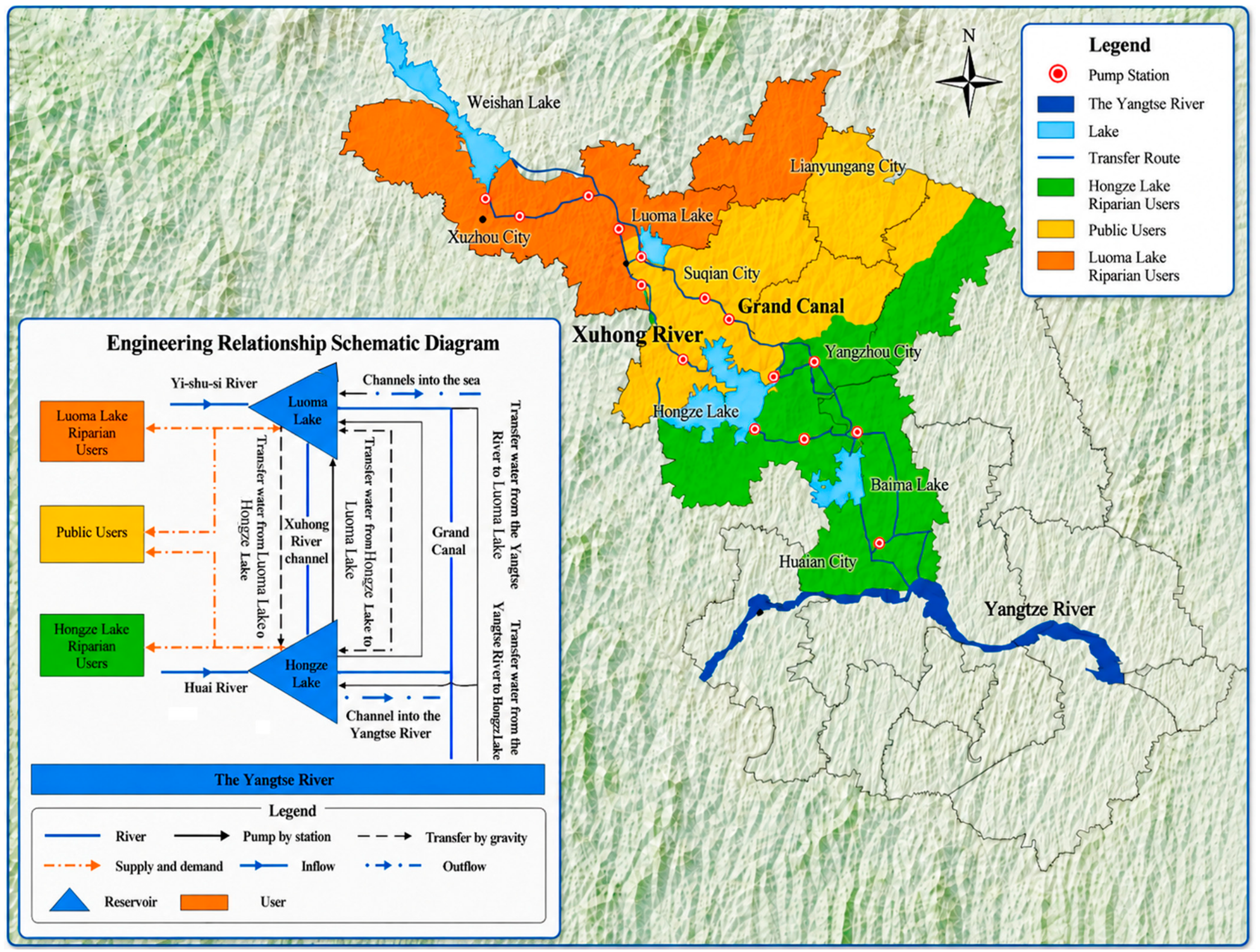
The study area is located in the water-receiving zone along the Beijing-Hangzhou Grand Canal in Jiangsu Province, eastern China, north of the main intake of the Eastern Route of the South-to-North Water Diversion Project (SNWDP-ER)—one of the world’s largest inter-basin water transfer schemes. The region covers approximately 43,143 km2, with irrigated agricultural land accounting for about 83% of the total area, making it a typical water-receiving region with high and composite water demand. The regional water supply system consists of two large shallow lakes (Hongze Lake and Luoma Lake) and the SNWDP-ER, with the Grand Canal and local plain river networks serving as the main conveyance channels. Together, they form a multi-source joint regulation system connecting the Yangtze River, Huai River and Yishusi river systems. Characterized by diverse water sources, complex conveyance routes and close hydraulic connections, the system exhibits typical features of multi-source, multi-user and multi-constraint coupling.
Hongze Lake, the fourth-largest freshwater lake in China, is the core regulating reservoir in the lower Huai River basin and receives natural inflow primarily from the Huai River system. Luoma Lake, another major shallow lake in northern Jiangsu, is mainly fed by the Yishusi river system (a combined system of the Yi, Shu and Si rivers). Local rainfall-runoff serves as the main source of interval runoff between the two lakes. Located in the climatic transition zone between the subtropical Huai River valley and temperate North China, the two lake basins have markedly asynchronous rainfall and inflow regimes, resulting in pronounced spatiotemporal heterogeneity of regional water resources.
Under conditions of uneven inflow distribution, Hongze Lake and Luoma Lake can exchange water bidirectionally via two main conveyance routes: the Xuhong River (a man-made waterway) and the Beijing-Hangzhou Grand Canal. Water transfer from Hongze Lake to Luoma Lake requires multi-stage pumping to overcome elevation differences, whereas replenishment from Luoma Lake to Hongze Lake occurs by gravity controlled by sluice gates. During consecutive dry years when local water resources are insufficient to meet demand, the SNWDP-ER is activated to divert water from the Yangtze River via the Jiangdu Pumping Station to recharge the regional system. Differences in inflow regime, storage regulation capacity, conveyance mode and operation rules among water sources further increase the complexity of the joint operation system.
The study area covers multiple prefecture-level cities including Xuzhou, Huai’an, Yangzhou and Suqian, serving a diverse range of water users: agricultural irrigation, industrial production, urban–rural domestic use and ecological replenishment. Water demand exhibits significant spatiotemporal heterogeneity, with users differing substantially in allocation priority, demand pattern and water consumption scale. The source–user relationship is not a simple one-to-one correspondence but a complex “multi-source–multi-user” coupled structure: some users are supplied by a single source, while shared receiving zones rely on joint supply from both Hongze Lake and Luoma Lake.
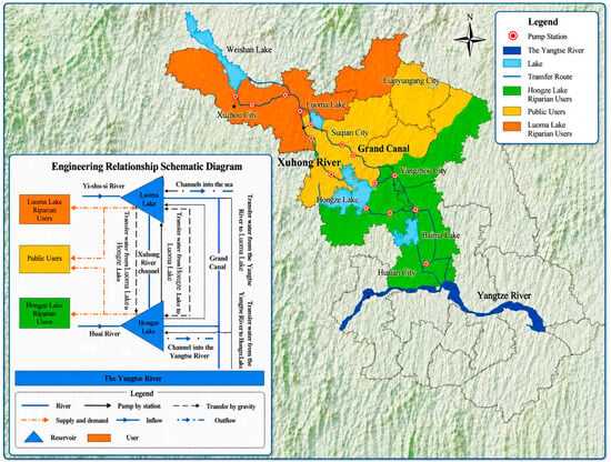
Driven by the complex conveyance network, complementary source relationships and dynamic multi-user demand, the regional joint operation system exhibits typical high-dimensional nonlinear MIMO characteristics. Traditional operation methods struggle to establish accurate dynamic mapping relationships between complex source inputs and multi-objective supply outputs. Based on the source–sink relationships and source–user coupling characteristics of the system, this study generalizes the Hongze Lake–Luoma Lake–SNWDP joint operation system, as illustrated in Figure 1.
Figure 1.
Generalized schematic of the water resources system in the Jiangsu section of the Eastern Route of the South-to-North Water Diversion Project.
3. Methodology
3.1. Data Sources and Preprocessing
The dataset consists of multi-year monthly hydrological operation records from the Hongze Lake–Luoma Lake–Yangtze Diversion system in the Jiangsu section of the SNWDP-ER. Input features include reservoir inflow, current storage volume, outflow discharge and user water demand; outputs are optimized water allocation discharges from each source to each user. Let the input feature dimension be f and the output dimension n = 3 (corresponding to three main user groups), with a total sample size N. The input and output variables of the MIMO mapping dataset are specified in Table 1.
Table 1.
Input and output variables of the MIMO mapping dataset.
The dataset is split chronologically into training and test sets at an 8:2 ratio to preserve the temporal dependencies inherent in hydrological series. Unlike random hold-out splitting, chronological division means the two subsets may differ in value range, extreme-event proportion and seasonal water supply characteristics; such distribution differences are critical for interpreting train–test performance gaps and cannot be simply equated to differences in model generalization ability. To characterize the statistical properties of both subsets and provide a baseline for subsequent generalization analysis, descriptive statistics including mean, standard deviation (Std), minimum (Min), maximum (Max), and total wet-/dry-season water supply are calculated for each of the three water-allocation outputs, and the results are summarized in Table 2.
Table 2.
Descriptive statistics of training and test subsets for three water allocation outputs.
Overall, the statistical characteristics of the three outputs are generally comparable between the training and test subsets. Specifically, the Hongze Lake supply output shows a moderately narrower value range and lower total wet-season water volume in the test subset, while Luoma Lake supply and Yangtze diversion supply show similar dispersion and extreme-value levels across the two subsets.
Given the large magnitude differences among water resources variables and legitimate extreme values during flood seasons, Z-score standardization is applied to both input and output data. Unlike min–max normalization, whose mapping range is entirely determined by extreme values, Z-score standardization is based on the mean and standard deviation, making it far less sensitive to outliers. It better expands the distribution range of normal-range data and improves the model’s discriminative ability across features of different scales. After standardization, the data are reshaped into a 4D tensor of [f, 1, 1, M] to match the input structure of the convolutional neural network. The sum of specific input features for each sample is recorded as the upper-bound reference for subsequent physical constraint post-processing.
where x is the raw sample value, μ is the feature mean, and σ is the feature standard deviation.
3.2. Convolutional Neural Network (CNN)
Convolutional neural networks extract local features via sliding convolutional kernels and reduce feature dimensionality via pooling operations, with strong automatic feature extraction capability in computer vision, natural language processing and time series analysis.
In multi-reservoir joint operation scenarios, the input feature matrix embeds important spatial correlation information, including hydraulic links between upstream and downstream reservoirs, and water competition/priority relationships among users. To address the limitation of traditional operation function methods in explicitly modeling the spatial topology of water supply networks, this study performs one-dimensional convolution along the source–user feature dimension.
The f input features are arranged along the physical conveyance path: source state variables are ordered from upstream to downstream (Hongze Lake, Luoma Lake, and the Yangtze diversion route), followed by user-side features ordered by allocation priority. Consequently, adjacent positions in the feature vector correspond to physically adjacent or directly interacting elements of the source–user chain, which gives the local 3 × 1 convolution kernels an explicit physical meaning.
Learnable convolutional kernels extract local spatial coupling patterns across adjacent feature dimensions, enabling the model to capture multi-level spatial dependencies in multi-source water supply networks. The one-dimensional convolution operation is formulated as:
where is the j-th raw input value in the sliding window corresponding to the i-th output position; is the j-th learnable weight parameter in the convolution kernel; k is the kernel size; b is the bias term; is the nonlinear activation function; and is the i-th convolution output value.
The ReLU function is adopted as the nonlinear activation function. Unlike sigmoid and tanh, ReLU maintains a constant gradient of 1 for x > 0, effectively mitigating the gradient vanishing problem in deep networks. It also features low computational cost and fast convergence, making it one of the most widely used activation functions in deep learning. It is defined as:
where x is the input value, and f(x) is the ReLU activation output.
A graph-based operator was considered but not adopted: it requires an adjacency matrix that, for this small and fixed near-linear conveyance chain, would have to be learned from a single network and would introduce substantially more parameters. The physically ordered feature vector, combined with local 1-D convolution, provides a parsimonious representation of the same local coupling relationships; a comparison with adaptive graph-attention operators is reserved for future work on larger, more densely connected networks.
3.3. Bidirectional Long Short-Term Memory (BiLSTM)
LSTM networks address the gradient vanishing and explosion problems of vanilla recurrent neural networks (RNNs) through three gating mechanisms: forget gate, input gate and output gate. This enables effective capture of long-range temporal dependencies in hydrological time series.
On this basis, Bidirectional LSTM (BiLSTM) consists of two parallel LSTM networks processing the input sequence in forward and reverse directions, simultaneously exploiting past and future contextual information. This overcomes the limitation of unidirectional LSTM, which can only utilize historical information.
In the context of reservoir joint operation, the forward LSTM processes the inflow–demand series in chronological order (t = 1 to T), modeling the cumulative effect of historical storage states on current scheduling decisions. The backward LSTM processes the same sequence in reverse order (t = T to 1), enabling the model to perceive the contextual dependencies within the historical window when read in reverse order. The forward and backward hidden states are concatenated to obtain a hidden layer representation fused with bidirectional temporal information. The model is trained as an offline retrospective mapping of historical operation records and is used for decision reference and scenario analysis, rather than as an autonomous real-time scheduler. The bidirectional temporal modeling mechanism and output representation of BiLSTM are formulated as:
where htforward and htbackward are the hidden states of the forward and backward LSTMs at time t, respectively; is the output hidden representation of BiLSTM at time t, integrating forward and backward temporal context; denotes the vector concatenation operation; and is the input feature vector at time t.
3.4. Sparrow Search Algorithm (SSA)
The Sparrow Search Algorithm is a swarm-intelligence optimization algorithm inspired by the foraging and anti-predation behaviors of sparrow flocks. The population is divided into three roles: producers, scroungers and scouts. Producers with higher fitness values are responsible for searching for optimal solutions in the search space and transmitting search direction information to the population. Scroungers follow producers for foraging and dynamically adjust their positions according to their fitness ranking. Scouts issue alarms when detecting search stagnation or local optimum threats, guiding the population to transfer to safer areas. The differentiated collaborative search of the three types of individuals achieves a good balance between global exploration and local exploitation, with fast convergence speed and high optimization accuracy.
where t is the current iteration number; is the maximum number of iterations; is the position of the i-th producer in the j-th dimension at iteration t; is a random number uniformly distributed in (0, 1]; is the alert value; is the safety threshold; Q is a random number following the standard normal distribution; and is a d-dimensional all-one vector. When , the search environment is safe and producers can conduct extensive search near their current positions; when , predators are detected and producers quickly fly to safe areas far from their current positions.
where is the current global optimal position; is the global worst position; is a d-dimensional matrix with elements randomly taking values of 1 or −1, and ; n is the total population size. When , scroungers with poor fitness conduct global diffusion search in the opposite direction of the global worst position in an exponential decay manner; otherwise, scroungers perform multi-directional local fine search near the current optimal position.
where is the global optimal position; is the step size control parameter following the standard normal distribution; K is a random number uniformly distributed in [−1, 1]; is a small constant to avoid division by zero; and are the current global best and worst fitness values, respectively; and is the fitness value of the i-th individual. When the scout’s fitness is better than the global optimal fitness, it conducts fine local search with small perturbations around the global optimum; when the scout’s fitness equals the global optimal fitness, it moves toward the global optimum to avoid danger. This alert mechanism enables the algorithm to effectively jump out of local optima in the later iteration stage and improve global convergence performance.
In MIMO mapping modeling for reservoir joint operation, the hyperparameter configuration of the CNN-BiLSTM hybrid architecture directly determines the prediction accuracy and generalization ability of the model, while traditional manual parameter tuning relies on expert experience and grid search faces the problem of dimensional explosion. The adaptive weighting mechanism assigns higher optimization weights to output dimensions with larger losses, guiding SSA to prioritize improving the underperforming outputs and enhancing the balanced prediction performance across multiple output dimensions.
3.5. SSA-CNN-BiLSTM Model Architecture
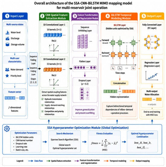
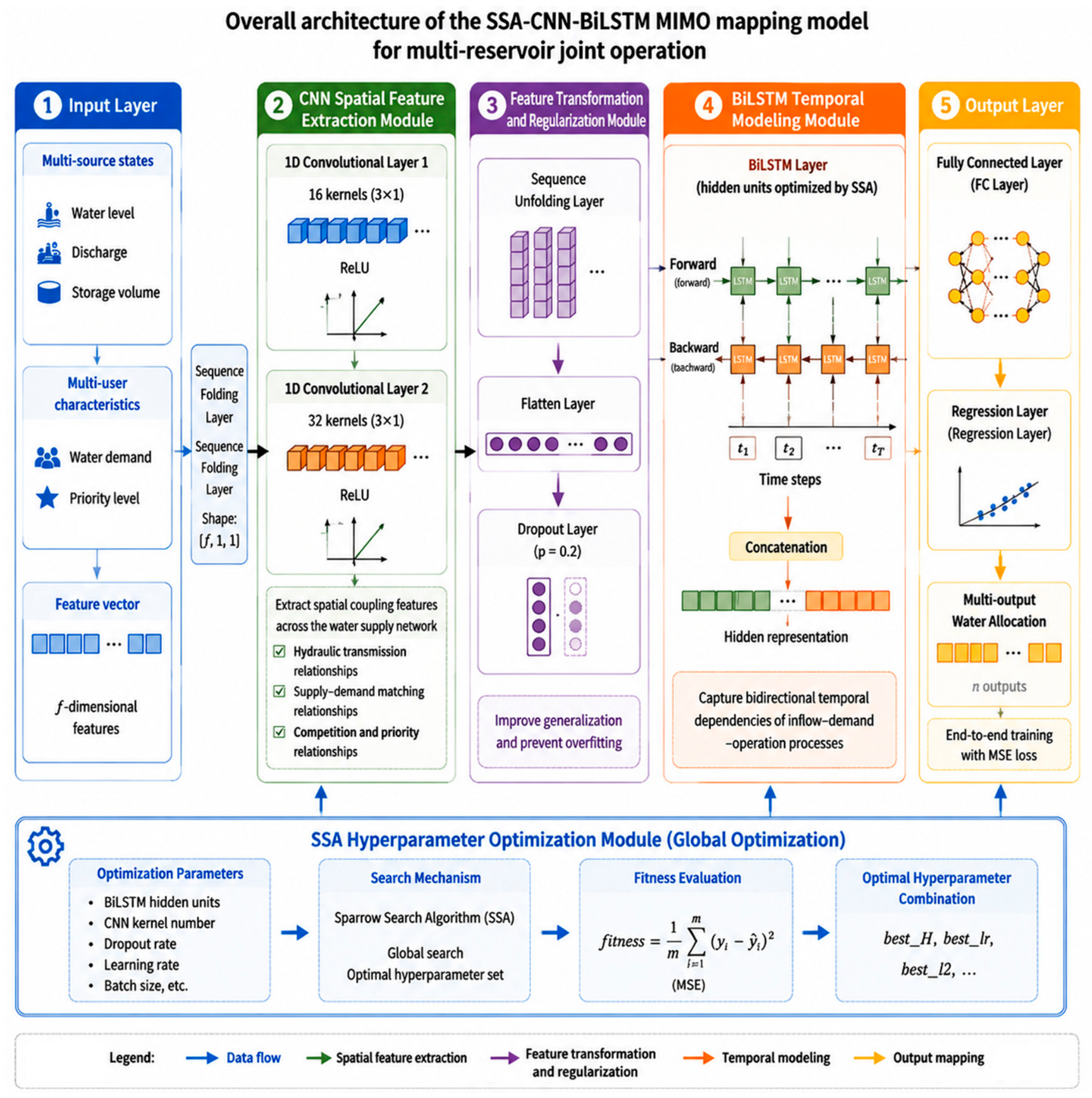
The overall architecture of the proposed SSA-CNN-BiLSTM MIMO mapping model for multi-reservoir joint operation is shown in Figure 2. It consists of five modules: input layer, CNN spatial feature extraction module, BiLSTM temporal modeling module, SSA hyperparameter optimization module and output layer. The model takes multi-source state variables (water level, discharge, storage volume, etc.) and multi-user characteristics (water demand, allocation priority, etc.) as inputs, and outputs optimized water allocation discharges from each source to each user. Through the synergy of CNN-based spatial feature extraction, BiLSTM-based temporal dependency capture and SSA-based global hyperparameter optimization, it realizes end-to-end MIMO mapping. This offline retrospective model learns mappings from historical reservoir operation records to support decision reference and scenario analysis, and it is not designed as an autonomous real-time scheduler. The specific structure is as follows:
Figure 2.
Overall framework of the SSA-CNN-BiLSTM multi-input multi-output mapping model for multi-reservoir joint operation.
- Input layer. The input data are f-dimensional feature vectors. A sequence folding operation is applied to reorganize batch samples into an image-sequence format with per time step folding within a 3-month sequence, overall tensor [batch, 3, f], where f is the input feature dimension, so that the subsequent one-dimensional CNN can perform convolution along the feature dimension.
- CNN spatial feature extraction. The folded data sequentially pass through two one-dimensional convolutional layers for feature extraction. The first layer uses 16 convolution kernels of size 3 × 1, followed by ReLU activation. The second layer uses 32 convolution kernels of size 3 × 1, also followed by ReLU activation. The two convolutional layers extract spatial coupling features of the water supply network along the source–user feature dimension, including hydraulic transmission relationships between upstream and downstream reservoirs, supply–demand matching relationships between water sources and users, and water competition and priority relationships among multiple users.
- Feature transformation and regularization. The CNN output is restored to a sequence structure via a sequence unfolding operation and compressed into a one-dimensional vector by a flatten layer. A dropout layer with a drop probability of 0.2 is inserted between the flatten layer and the BiLSTM layer: during training, 20% of neurons are randomly deactivated to enhance generalization; during inference, all neurons are activated, which is equivalent to ensembling the predictions of multiple sub-networks.
- BiLSTM temporal modeling. The flattened feature vectors are fed into the BiLSTM layer for bidirectional temporal modeling. The number of hidden units of the BiLSTM is automatically optimized by SSA, and the output mode is set to last-step sequence output. The forward LSTM processes the sequence in chronological order, modeling the cumulative effect of historical storage states and previous water supply decisions on the current scheduling scheme. The backward LSTM processes the same sequence in reverse order, enabling the model to perceive the contextual dependencies within the historical window when read in reverse order. Finally, the forward and backward hidden states are concatenated to achieve complete bidirectional modeling of the temporal dependencies of the inflow–demand process.
- Output layer. A fully connected layer maps the hidden representation of BiLSTM to n-dimensional water allocation outputs, and a regression layer performs end-to-end training with mean squared error (MSE) as the loss function. The network directly maps multi-dimensional input features to multi-output water allocations in a unified MIMO manner, without the need to build separate models for each output.
3.6. Training Strategy and Evaluation Metrics
The model is trained using the Adam optimizer with the following main configuration: maximum 500 training epochs; batch size of 512; piecewise constant learning rate decay with a decay factor of 0.1 and a decay period of 400 epochs; training data are shuffled before each epoch to improve generalization.
To prevent model overfitting, the following five strategies are comprehensively adopted:
- Dropout regularization: A dropout layer with a rate of 0.2 is inserted between the flatten layer and the BiLSTM layer. During training, 20% of neurons are randomly deactivated, forcing the network to learn robust features rather than memorizing training noise.
- L2 regularization: The L2 regularization coefficient is automatically optimized by SSA within the range [1 × 10⁻⁵, 0.8], which constrains model complexity by adding a weight squared sum term to the loss function.
- Validation-set early stopping: 10% of the samples from the end of the training set are reserved as the validation set. Training is terminated early if the validation loss does not decrease for 10 consecutive epochs.
- Gradient clipping: The gradient threshold is set to 1, which clips the L2 norm of gradients to no more than 1. This prevents gradient explosion and drastic parameter jumps caused by extreme samples, and maintains a smooth decline of the loss curve during training.
- Z-score standardization: Compared with min–max normalization, it reduces sensitivity to extreme values, fully expands the distribution range of normal data, and reduces gradient fluctuations during training.
To comprehensively evaluate the prediction performance of the model in MIMO multi-output scenarios, five evaluation metrics are adopted:
- Root Mean Square Error (RMSE): Measures the square root of the average squared deviation between predicted and true values.
- Coefficient of Determination (R2): Measures the proportion of variance explained by the model, ranging from (−∞, 1]; values closer to 1 indicate better fitting performance.
- Mean Absolute Error (MAE): The mean of absolute prediction errors, with a linear penalty on errors.
- Mean Absolute Percentage Error (MAPE): The relative error in percentage, facilitating accuracy comparison across outputs of different magnitudes.
- Mean Squared Error (MSE): The mean of squared prediction errors.
3.7. Physical Constraint Post-Processing
A fundamental physical constraint in water resources scheduling is that the sum of water allocations from all sources to all users must not exceed the total available water supply. A two-stage constraint correction strategy is applied to the model’s predicted outputs to ensure physical feasibility.
where is the model-predicted allocation of the j-th output component; is the total available water supply for sample s, calculated from the sum of lake water storage, river inflow and planned water transfer volume.
We further clarify that is derived from historically feasible operation records and therefore already reflects the storage regulation and conveyance capacities of the Xuhong River and the Grand Canal. Embedding the complete two-lake water-balance equations (inflow, storage change, losses) and explicit channel-capacity limits directly into the correction layer is stated as future work toward the closed-loop framework.
Stage 0—Non-negativity clipping: All predicted allocation values are clipped at zero to eliminate any physically meaningless negative outputs. For the present dataset, no raw predictions fall below zero, so this step acts as a passive safeguard rather than an active correction. It is applied prior to the upper-bound constraint correction to ensure numerical validity of subsequent scaling operations.
Stage 1—Proportional scaling: If the sum of n outputs for a sample exceeds the constraint upper bound, all outputs are scaled down proportionally until the sum satisfies the constraint.
where is the corrected allocation of the j-th component after proportional scaling.
Stage 2—Residual deduction: If minor violations still exist due to floating-point precision limitations, the residual excess is deducted only from the largest output component, as the largest output is most likely the main contributor to the violation.
where m is the index of the component with the largest scaled allocation, and the term in parentheses on the right-hand side is the small positive residual remaining after Stage 1 proportional scaling.
Deducting the residual only from the largest component minimizes the relative distortion introduced; an absolute deduction changes a large component by the smallest percentage, preserves the accuracy of the well-predicted small components, and avoids requiring sample-specific priority weights. Proportional and priority-based deduction schemes are noted as future refinements.
This two-stage “proportional scaling + residual deduction” strategy avoids the excessive correction of well-predicted small-output components that occurs with traditional pure proportional scaling methods.
4. Case Study
4.1. SSA Optimization Results and Model Training
The SSA optimization algorithm parameters are set as follows: population size of 30, maximum 200 iterations. The search ranges for the hyperparameters to be optimized are: number of BiLSTM hidden units [2, 200], initial learning rate [1 × 10⁻⁴, 0.3], L2 regularization coefficient [1 × 10⁻⁵, 0.8].
The fitness function adopts an adaptive weighted multi-output loss function, which normalizes and adaptively weights the combined RMSE and MAE loss of each output dimension. Output dimensions with larger losses are assigned higher weights, guiding SSA to prioritize improving the underperforming outputs and enhancing the balanced prediction performance across multiple output dimensions.
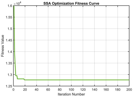
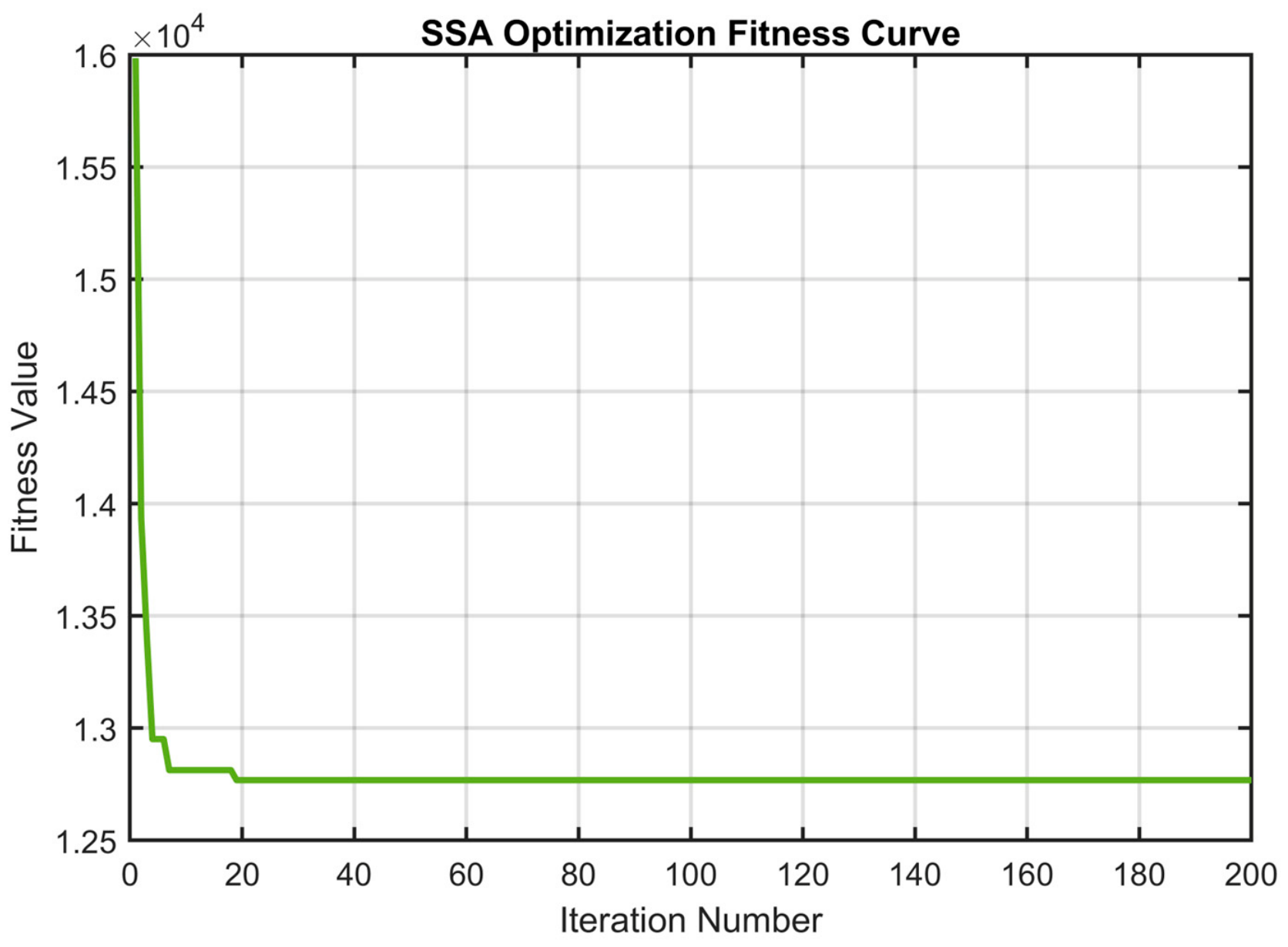
The SSA optimization fitness curve is shown in Figure 3. The fitness value decreases rapidly in the early iteration stage, indicating that SSA has high global search efficiency and can quickly locate high-quality regions in the parameter space. Subsequently, the algorithm enters a gradual convergence stage with a slowing fitness decline rate, and stabilizes around the 45th generation. No prolonged stagnation or severe oscillation occurs throughout the process, demonstrating good global convergence performance and search stability.
Figure 3.
Fitness curve of SSA optimization.
Through SSA global joint optimization, the optimal hyperparameter combination is obtained: the number of BiLSTM hidden units, initial learning rate and L2 regularization coefficient are all automatically tuned. The three key hyperparameters are jointly optimized under a unified SSA framework, effectively avoiding the subjectivity of manual empirical parameter tuning, the combinatorial explosion problem of grid search in continuous parameter spaces, and the decoupling of hyperparameter interaction effects in stepwise independent optimization. The hyperparameter settings of the proposed SSA-CNN-BiLSTM model and the baseline CNN-BiLSTM model are summarized in Table 3.
Table 3.
Hyperparameter configuration of the proposed model and comparative baselines.
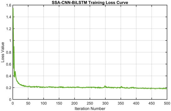
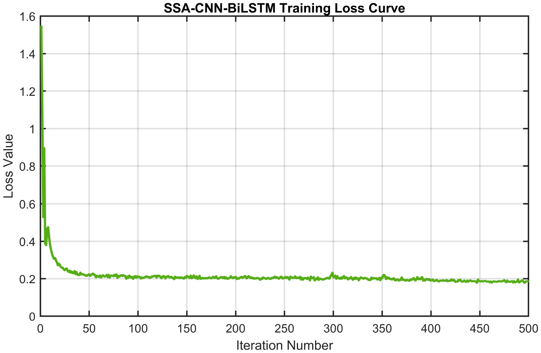
During model training, the loss function curve declines smoothly (Figure 4), with no obvious severe oscillation or spikes. This indicates that the algorithm effectively suppresses the gradient explosion problem caused by extreme samples, and the training process is stable and controllable. The validation set loss monitoring and early stopping mechanism ensure that training is terminated in time when validation performance no longer improves, avoiding unnecessary computational resource consumption and over-training risks.
Figure 4.
Training loss curve of the SSA-CNN-BiLSTM model.
4.2. Prediction Performance Analysis
Table 4 summarizes the prediction performance evaluation metrics of the model on the training and test sets. To comprehensively evaluate the per-output prediction capability and overall generalization performance in the MIMO multi-output scenario, six evaluation metrics (RMSE, R2, MAE, MAPE, MSE and PBIAS) for each output dimension on the training and test sets, as well as the three-output average, are calculated separately.
Table 4.
Prediction performance metrics of the SSA-CNN-BiLSTM model.
As can be seen from Table 4, the SSA-CNN-BiLSTM model achieves satisfactory prediction performance across all three output dimensions. The overall average test R2 of the three outputs is 0.8637 and the average test MAPE is 20.61%, indicating that the model successfully establishes an end-to-end MIMO nonlinear mapping relationship from multi-source state variables and multi-user demand characteristics to the optimized water allocation of each user. There are certain performance differences among output dimensions, and the per-output analysis is as follows.
- Hongze Lake water supply prediction. The test set R2 is 0.9403 and MAPE is 19.26%, indicating that the model has high mapping accuracy for this output dimension and can directly provide reliable reference for practical scheduling decisions. The R2 difference between the training set and test set is negligible, indicating excellent generalization performance. Notably, the test set MAPE is 2.68 percentage points lower than that of the training set, and the test set RMSE and MAE are also lower than the corresponding values of the training set. The slightly lower test errors are mainly attributable to the narrower value range and lower wet-season mean of the test period (Table 2); combined with the small train–test gap, they indicate an absence of severe overfitting rather than a test fit superior to the training fit. The Hongze Lake water supply prediction spans more than one order of magnitude in the training set, and the model maintains stable prediction accuracy across such a wide numerical range. This verifies the strong fitting ability of the synergy between CNN spatial feature extraction and BiLSTM bidirectional temporal modeling for the complex nonlinear relationship of water allocation.
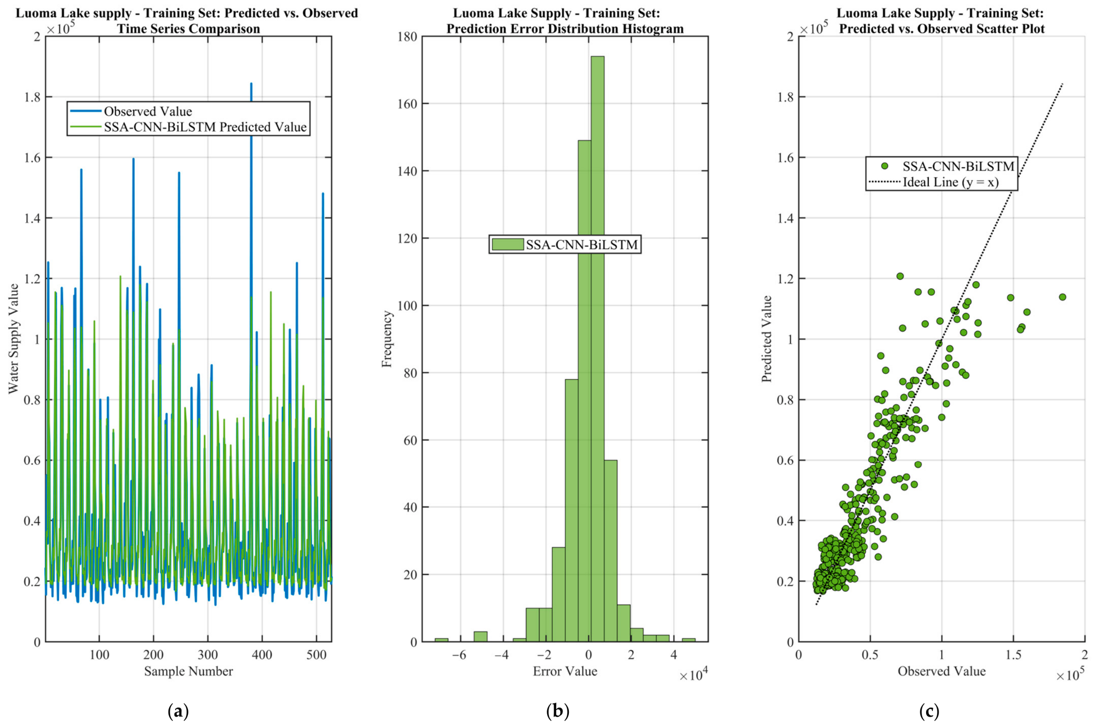
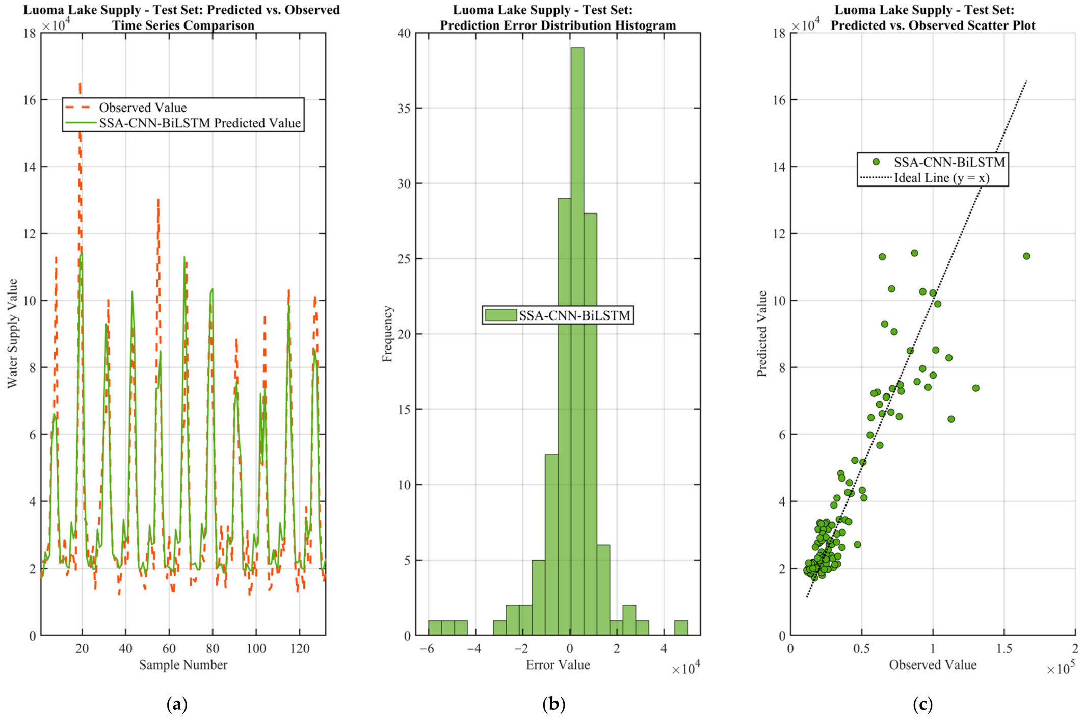
- Luoma Lake water supply prediction. The test set R2 is 0.8114 and MAPE is 22.29%, representing moderate accuracy. Among the three output dimensions, Luoma Lake supply shows the most obvious overfitting tendency: the R2 difference between training and test sets exceeds the 0.03 warning threshold; four generalization metrics show consistent degradation—test set RMSE increases by 2290.4, MAE increases by 1019.4, MAPE rises by 2.37 percentage points, and R2 decreases by 0.0424—forming consistent evidence for generalization degradation. The underlying cause may be that the allocation pattern corresponding to this output is more complex, or the training samples have insufficient coverage of this pattern, leading the model to partially memorize training noise rather than fully learning the true data generation rules. Nevertheless, the RMSE/MAE ratio of Luoma Lake water supply prediction is 1.58, well below the 2.0 outlier warning threshold, indicating that the prediction errors are generally normally distributed and there is no problem of a small number of large-error samples dominating the overall error. Subsequent overfitting mitigation measures may include appropriately increasing the dropout rate, increasing the L2 regularization coefficient, or reducing the early stopping patience value to trigger early stopping earlier.
- Yangtze diversion water supply prediction. The test set R2 is 0.8393 and MAPE is 20.29%, representing medium-to-high accuracy. The training and test generalization performance of Yangtze diversion water supply is good and stable: the R2 change is not significant; RMSE increases slightly from 14,976.3 to 15,887.8; MAE increases marginally from 10,795.5 to 10,891.0, with an almost negligible increase; while MAPE improves from 22.50% to 20.29%, with the test set relative error outperforming the training set. Overall, Yangtze diversion supply has good and stable generalization performance and can meet the operational needs of water allocation decision-making. In addition, the RMSE/MAE ratio of Yangtze diversion water supply prediction is 1.46, the lowest among the three outputs, indicating that its error distribution has the smallest dispersion and the highest prediction consistency.
4.3. Prediction Visualization and Error Analysis
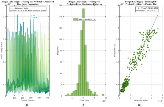
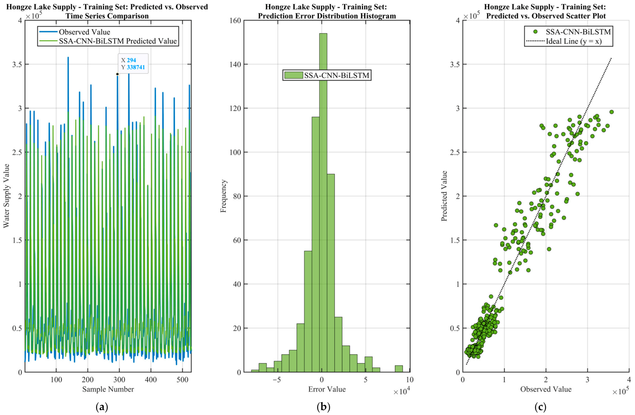
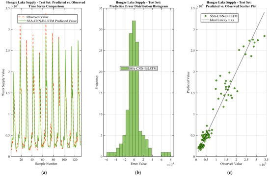
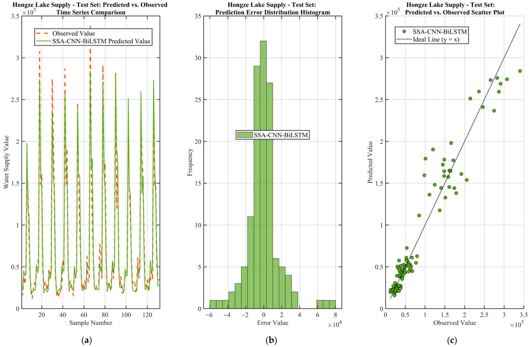
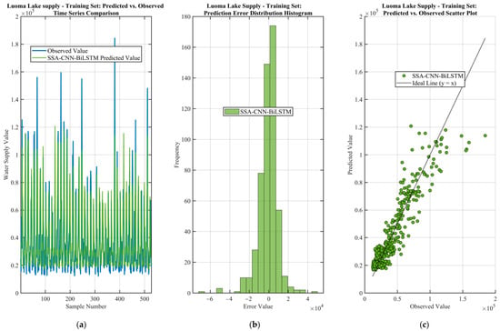
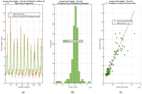
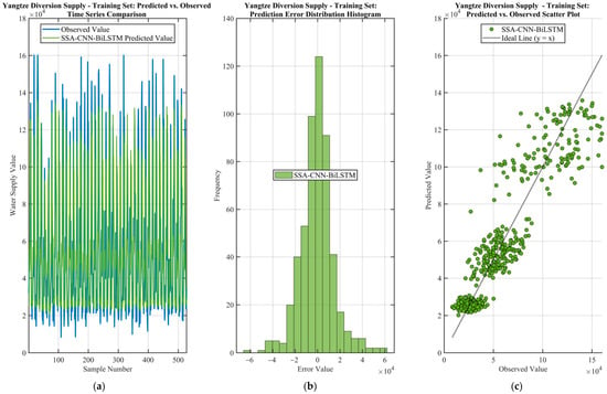
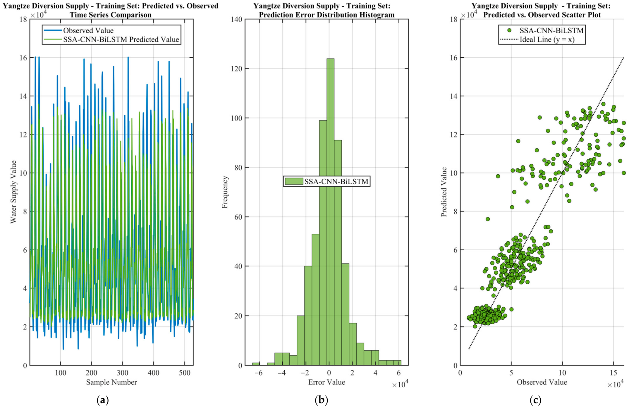
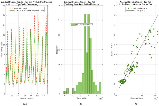
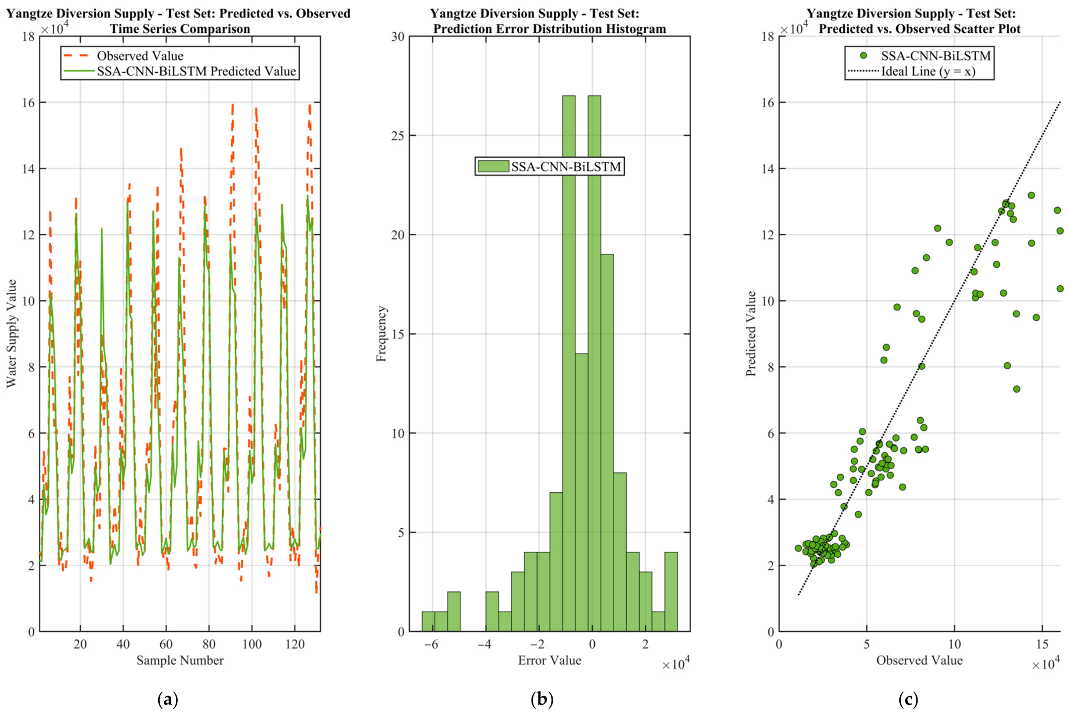
To intuitively demonstrate the prediction effect of the model on multiple output dimensions, Figure 5, Figure 6, Figure 7, Figure 8, Figure 9 and Figure 10 present three sets of visualization results for the three water source supplies on the training and test sets respectively: predicted vs. true value time-series comparison curves (subfigure a), prediction error distribution histograms (subfigure b), and predicted vs. true value scatter fitting plots (subfigure c).
Figure 5.
Prediction performance of Hongze Lake water supply on the training set: (a) Time-series comparison of predicted and observed values; (b) Prediction error distribution histogram; (c) Scatter plot of predicted vs. observed values.
Figure 6.
Prediction performance of Hongze Lake water supply on the test set: (a) Time-series comparison of predicted and observed values; (b) Prediction error distribution histogram; (c) Scatter plot of predicted vs. observed values.
Figure 7.
Prediction performance of Luoma Lake water supply on the training set: (a) Time-series comparison of predicted and observed values; (b) Prediction error distribution histogram; (c) Scatter plot of predicted vs. observed values.
Figure 8.
Prediction performance of Luoma Lake water supply on the test set: (a) Time-series comparison of predicted and observed values; (b) Prediction error distribution histogram; (c) Scatter plot of predicted vs. observed values.
Figure 9.
Prediction performance of Yangtze diversion water supply on the training set: (a) Time-series comparison of predicted and observed values; (b) Prediction error distribution histogram; (c) Scatter plot of predicted vs. observed values.
Figure 10.
Prediction performance of Yangtze diversion water supply on the test set: (a) Time-series comparison of predicted and observed values; (b) Prediction error distribution histogram; (c) Scatter plot of predicted vs. observed values.
From the prediction comparison curves (Figure 5a, Figure 6a, Figure 7a, Figure 8a, Figure 9a and Figure 10a), the predicted value curves and true value curves are highly consistent in overall trend, and can accurately track the complete temporal change process of each output water allocation. The model tracks the timing of wet-season allocation peaks without systematic phase shift, although the magnitudes of the highest Luoma Lake peaks are moderately underestimated and the low-value clusters show larger scatter (quantified below). To quantify peak prediction accuracy, the mean relative error (MRE) of the 10 highest observed values is calculated for each output: 9.3% for Hongze Lake supply, 22.2% for Luoma Lake supply, and 22.6% for Yangtze diversion supply. In the low-value valley intervals of dry seasons, the predicted values also closely fit the true values. This indicates that BiLSTM bidirectional temporal modeling effectively extracts the long-range temporal dependencies of the inflow–demand process, and the model has good mapping ability for water allocation decisions under extreme hydrological conditions.
From the error distribution histograms (Figure 5b, Figure 6b, Figure 7b, Figure 8b, Figure 9b and Figure 10b), the prediction errors of all three outputs on both training and test sets show an approximately normal distribution, centered near zero, with good left-right symmetry and thin distribution tails. This distribution characteristic indicates that the model prediction has no systematic bias, the prediction errors of most samples are concentrated near the mean, and extreme errors occur at low frequency. The error distribution concentration of the three water source supplies ranks from high to low: Hongze Lake supply, Yangtze diversion supply, Luoma Lake supply, which is consistent with the performance ranking of R2 for each output.
From the scatter fitting plots (Figure 5c, Figure 6c, Figure 7c, Figure 8c, Figure 9c and Figure 10c), the predicted-true value scatter points of all outputs are tightly distributed on both sides of the ideal fitting line y = x. The degree of deviation increases slightly with increasing values, showing mild heteroscedasticity, which is consistent with the natural attribute of water allocation data that “large values have greater fluctuations than small values”. The scatter band of Hongze Lake supply is the narrowest and has the highest fit to the ideal line; the scatter points of Luoma Lake supply are slightly dispersed in the low-value interval, which partly explains its lower R2, i.e., the relatively large relative error in the low-value interval leads to higher MAPE; Yangtze diversion supply is intermediate between the two.
Further, using ±15% relative error as the criterion, the prediction qualification rates on the test set are counted: 44.7% for Hongze Lake supply, 43.2% for Luoma Lake supply, and 38.6% for Yangtze diversion supply. Because small-magnitude samples are frequent in dry seasons and intrinsically inflate percentage error, looser thresholds are more informative for engineering use: at ±25% the rates rise to 72.0%, 59.8% and 67.4%, and at ±50% to 93.9%, 92.4% and 97.0%. These results indicate that large relative errors are concentrated on low-allocation samples, whereas bulk allocations are captured substantially better.
The bimodal scatter pattern in Figure 9c and Figure 10c arises from two distinct operation regimes embedded in the historical records: routine water supply under normal conditions, and flood-season emergency transfer with mixed pumped and gravity conveyance. These two regimes form separate value clouds in the scatter plot. The upward spread of the low-value cloud is a typical regression-to-the-mean effect for small-magnitude samples, which is consistent with the MAPE pattern discussed earlier. Regime-conditional modeling will be investigated in future work to further improve low-value prediction accuracy.
4.4. Overfitting Diagnosis and Model Generalization Assessment
To systematically evaluate the generalization state of the model on each output dimension, an internal descriptive screening is applied based on the differences between training set and test set evaluation metrics, and the results are summarized in Table 5. These cut-offs are empirical heuristics for this dataset rather than universal criteria. The diagnosis logic is as follows: if ΔR2 (training R2 − test R2) > 0.03 or ΔMAPE (test MAPE − training MAPE) > 3 percentage points, it is marked as “suspected mild overfitting”; if ΔR2 < −0.02, it is marked as “excellent generalization (test > training)”; if |ΔR2| ≤ 0.01 and ΔMAPE < 1 percentage point, it is marked as “good generalization, no overfitting”. Meanwhile, the RMSE/MAE ratio is calculated as an auxiliary criterion for outliers: a ratio much greater than 1 indicates the presence of a small number of large-error extreme samples.
Table 5.
Overfitting/underfitting diagnosis results.
The diagnosis results show that Hongze Lake supply prediction and Yangtze diversion supply prediction have stable generalization performance. For Hongze Lake supply prediction, ΔR2 is extremely small and both ΔRMSE and ΔMAE are negative. As shown in Table 2, the test subset has a narrower value range, which partly explains the lower test errors. The small performance gap between training and test sets demonstrates that the model avoids severe overfitting under the given regularization strategy. For Yangtze diversion supply prediction, the four Δ indicators have negligible changes and the generalization performance is stable and reliable. Luoma Lake supply prediction is marked as suspected mild overfitting, with four indicators forming consistent evidence pointing to generalization degradation. However, the degree of overfitting is still mild and the model still has certain practical value. Notably, the RMSE/MAE ratios of all three outputs do not exceed the 2.0 outlier threshold, indicating that the error distribution of each output is uniform and there is no problem of large-error extreme samples contaminating the overall evaluation.
Based on the test set R2, each output dimension is rated into four performance levels (A to D) as an empirical grading for internal comparison, and the accuracy is annotated in combination with MAPE (MAPE < 20% for high accuracy, 20–25% for medium accuracy, >25% for low accuracy). The results are shown in Table 6.
Table 6.
Performance grading results for each output.
The overall model health is rated as good: the average test R2 of the three outputs is 0.8637, the average test MAPE is 20.61%, and one out of three outputs shows mild overfitting. The evaluation conclusion is that the model has good overall generalization ability, basically balanced performance across output dimensions, and can be put into use directly or after light fine-tuning. It is recommended to adopt the aforementioned overfitting mitigation measures for Luoma Lake supply—appropriately increasing the dropout rate to 0.3–0.4, increasing the L2 regularization coefficient, or reducing the early stopping patience value to trigger early stopping earlier—and then retrain to further improve the overall performance and balance across output dimensions.
4.5. Physical Constraint Compliance Analysis
To verify whether the model prediction results satisfy the physical feasibility constraint that “the sum of water allocations from all sources to all users shall not exceed the total available water supply”, the two-stage constraint correction strategy is applied to the raw model outputs.
Constraint correction statistics show that the proportion of samples requiring constraint correction is 2.15% for the training set and 3.42% for the test set. The mean and maximum correction magnitude are 12.64 and 78.31 (104 m3), indicating good physical consistency of the model prediction results. The raw prediction results of most samples naturally satisfy the total available water supply constraint, and only a very small number of boundary operating conditions require slight correction. This result is of great significance: it verifies that the CNN-BiLSTM deep learning model can automatically learn implicit physical constraint rules from historical operation data in a data-driven manner, even without explicitly introducing physical constraints as training loss terms. Since historical operation data themselves are feasible solutions satisfying physical constraints, the model naturally internalizes the constraint boundaries by learning these feasible solutions.
From the statistical characteristics of the total output water allocation, the average true value sum of the three outputs in the training set is 173,396, and the average predicted sum is 171,941, with an average deviation of −1454.9. In the test set, the average true value sum is 170,545.9, and the average predicted sum is 167,133.5, with an average deviation of −3412.4. Both deviations are slightly negative, indicating that the model prediction results are generally conservative, tending to slightly underestimate rather than overestimate water allocations.
This conservative characteristic has positive safety implications in practical scheduling decisions: slight underestimation can be compensated by reserving safety margins and will not cause systemic risk of water supply shortage. In contrast, systematic overestimation may lead to infeasible scheduling schemes that exceed the available water supply capacity, bringing hidden dangers to water supply security. The two-stage constraint correction strategy first ensures boundary constraints through “proportional scaling”, and then deducts only from the largest output component for minor violations caused by floating-point precision through “residual deduction”. This effectively avoids the disproportionate distortion of small-output components caused by traditional pure proportional scaling methods, so that the prediction accuracy of each output component can be maintained independently.
4.6. Comparative Analysis with Alternative Models
To verify the superiority of the SSA-CNN-BiLSTM hybrid model compared with other typical model architectures, three comparative models are constructed and evaluated on the same dataset: (1) standalone BiLSTM model (without CNN spatial feature extraction module); (2) CNN-LSTM model (replacing BiLSTM with unidirectional LSTM); (3) vanilla CNN-BiLSTM model without SSA optimization (hyperparameters adopt empirical default values). All comparative models adopt the same data partitioning, standardization method and training configuration as the proposed model to ensure comparability. The empirical default hyperparameters of the vanilla CNN-BiLSTM baseline (without SSA optimization) are hidden units = 100, initial learning rate = 1 × 10⁻³, and L2 regularization coefficient = 1 × 10⁻⁴. The comparison results are shown in Table 7.
Table 7.
Performance comparison of different model architectures (multi-source test-set average).
Comparative analysis shows that:
- The contribution of the CNN spatial feature extraction module is the most significant. After introducing CNN, R2 increases from 0.7763 (BiLSTM) to 0.8149 (CNN-LSTM) (+0.0386), and RMSE decreases by 1795, verifying the critical role of CNN-extracted local source–user coupling features induced by the physically ordered feature vector in MIMO mapping modeling.
- BiLSTM bidirectional temporal modeling further improves prediction accuracy compared with unidirectional LSTM. R2 increases from 0.8149 (CNN-LSTM) to 0.8453 (CNN-BiLSTM) (+0.0304), and RMSE decreases by 1552, indicating that capturing bidirectional temporal dependencies brings substantial benefits to inflow–demand process modeling.
- SSA global joint auto-optimization further improves the performance of CNN-BiLSTM. R2 increases from 0.8453 to 0.8637 (+0.0184), RMSE decreases by 1015, and MAPE decreases by 1.12 percentage points. This suggests that SSA-based joint tuning can find a favorable configuration for the CNN-BiLSTM model; a multi-seed statistical comparison is needed in future work to quantify run-to-run variability.
From BiLSTM to SSA-CNN-BiLSTM, R2 increases by 0.0874 cumulatively and RMSE decreases by 4362 cumulatively (a 21.9% reduction). The performance gains from the three improvement strategies are consistent in direction and additive, jointly constituting a complete performance improvement pathway. The computational cost of the SSA hyperparameter search is supplemented as follows: the full SSA search took 176 min over 6030 fitness evaluations on an NVIDIA GeForce RTX 4060 Laptop GPU (8 GB), and final-model training took 0.02 min.
5. Discussion
The case study results show that the SSA-CNN-BiLSTM model achieves good MIMO mapping performance on multi-year monthly operation data of the Hongze Lake–Luoma Lake–Yangtze Diversion system in the Jiangsu section of the SNWDP-ER, with an average test R2 of 0.8637 and an average MAPE of 20.61%.
5.1. Comparison with Relevant Studies
Owing to the distinct task scopes and output indicators, a direct quantitative comparison of evaluation metrics across these studies is not appropriate. Each approach demonstrates unique advantages in its targeted application context, as summarized in Table 8: graph attention and Transformer architectures are particularly effective for capturing spatial topological relationships and closed-loop operational control. In contrast, the proposed model is tailored for the understudied many-to-many source–user water allocation mapping task, on which it achieves an average test R2 of 0.8637.
Table 8.
Summary comparison with previously published reservoir operation studies.
5.2. Output Performance Difference Analysis
We hypothesize that the performance differences among the three output dimensions are associated with the inherent differences in the complexity of water allocation schemes for different users in actual water resources scheduling systems. Users corresponding to Hongze Lake may have relatively stable demand processes and clear allocation rules, which may contribute to high signal-to-noise ratio historical data that CNN-BiLSTM can efficiently extract. The water allocation decisions for users corresponding to Luoma Lake are likely affected by the coupling of more time-varying factors, such as the disturbance of seasonal water use peaks to allocation rules, the dynamic adjustment of multi-source competition patterns, and the indirect transmission effect of upstream reservoir storage and release strategies. This would presumably lead to relatively low information density of training data, insufficient signal-to-noise ratio of effective patterns, and greater learning difficulty. This mechanistic explanation is presented explicitly as a hypothesis, and will be tested with series-level statistics including coefficient of variation (CV), extreme-month counts and lag-1 autocorrelation in future work.
This phenomenon is universal in MIMO deep learning modeling: different output dimensions naturally present unequal predictability due to the inherent complexity differences of data generation mechanisms. The adaptive weighting mechanism introduced in the SSA fitness function in this paper is an effective mitigation strategy for this problem, preventing the optimization process from being dominated by easy-to-predict advantageous outputs while ignoring difficult-to-predict disadvantageous outputs.
5.3. Methodological Framework and Quality Assurance
From a methodological perspective, the comprehensive training strategy system adopted in this study can be summarized as a five-stage quality assurance framework: preprocessing → regularization → optimization → constraint → descriptive screening. Specifically: Z-score standardization (reducing outlier sensitivity) → CNN spatial feature extraction + BiLSTM bidirectional temporal modeling (representation learning at the network structure level) → dropout regularization + L2 regularization (complexity constraint at the training level) → validation set early stopping + gradient clipping (stability guarantee at the optimization level) → physical constraint post-processing (feasibility guarantee at the output level) → internal descriptive screening system (quality monitoring at the evaluation level). Each link complements and synergizes with the others, jointly ensuring the generalization ability and output quality of the model in complex MIMO scenarios. The case study results verify the effectiveness of this comprehensive strategy system. Ablation experiments of each individual strategy (quantifying the independent contribution of each strategy by removing or disabling them one by one) and factorial analysis of the interaction effects among strategies can serve as important directions for in-depth follow-up research.
5.4. Limitations
Several limitations of this study should be acknowledged. First, the model operates at a monthly time step and therefore cannot resolve event-scale or daily scheduling decisions. Second, it is validated on a single, near-linear source–user network; transfer to larger and more densely connected systems remains to be tested. Third, no uncertainty quantification is provided: the SSA and network training are stochastic, and run-to-run variability (mean and standard deviation over repeated seeds) is not yet quantified. Fourth, the learned mapping is compared with alternative data-driven architectures but not with optimization-based scheduling schemes (e.g., genetic algorithms or mixed-integer programming). Fifth, the spatial features of the 1-D CNN depend on the chosen ordering of the feature vector, and order-permutation ablation has not yet been performed; a graph-based operator that learns adjacency is a natural alternative. Finally, the record length is limited, and the test period contains fewer extreme events than the training period.
5.5. Future Work
These limitations define our future work: (i) repeated training (≥10 random seeds) with mean ± standard deviation and statistical tests of inter-model differences; (ii) feature-order permutation ablation and a controlled comparison with graph neural operators such as adaptive graph attention; (iii) head-to-head benchmarking of SSA against PSO, GWO and Bayesian optimization under matched evaluation budgets; (iv) embedding the full two-lake water balance and channel-capacity constraints into the model, together with non-negativity guarantees; (v) comparison with optimization-based scheduling and, ultimately, coupling the mapping model with evolutionary optimization frameworks to form a complete decision support pipeline.
6. Conclusions
Aiming at the complex modeling problem of multi-source multi-user mapping in multi-reservoir joint operation, this paper proposes an SSA-CNN-BiLSTM MIMO mapping model for multi-reservoir joint operation, which is validated with multi-year monthly operation data of the Hongze Lake–Luoma Lake–Yangtze Diversion system in the Jiangsu section of the SNWDP-ER. The case study results show that the model achieves an average test R2 of 0.8637 and an average MAPE of 20.61% for the overall water supply output. Among them, Hongze Lake supply achieves a test R2 of 0.9403, Yangtze diversion supply reaches 0.8393, and Luoma Lake supply is 0.8114. The overall generalization performance is good with no severe overfitting. The main conclusions are as follows:
- The CNN-BiLSTM hybrid provides an effective MIMO mapping for multi-source multi-user allocation: on the held-out test period, the average R2 reached 0.8637 (0.9403, 0.8114 and 0.8393 for Hongze Lake, Luoma Lake and Yangtze diversion supply), i.e., above 0.81 for every output.
- The controlled architecture comparison shows consistent, additive gains: CNN spatial-feature extraction raised R2 by 0.0386, bidirectional temporal modeling by a further 0.0304, and SSA joint hyperparameter optimization by 0.0184; cumulatively R2 rose by 0.0874 and RMSE fell by 21.9% relative to the plain BiLSTM.
- Generalization was acceptable rather than perfect: two outputs showed stable train–test agreement while the Luoma Lake output showed mild overfitting; after the two-stage physical correction, the mean total allocation deviation was −0.84% (training) and −2.00% (test), i.e., slightly conservative, and the share of corrected samples was below 5% (2.15% training, 3.42% test).
- The model is a mapping-simulation reference for multi-source allocation analysis; the integrated “state perception–mapping simulation–optimal decision” framework requires coupling with optimization-based scheduling and is left as future work.
The main contributions of this study are: (a) adapting the SSA-CNN-BiLSTM architecture to MIMO mapping for multi-source multi-user reservoir joint operation and representing local source–user coupling features with a 1-D CNN over a physically ordered feature vector; (b) demonstrating a swarm-intelligence-based joint optimization of the key heterogeneous CNN-BiLSTM hyperparameters as an alternative to manual and grid-search tuning; and (c) showing, on the Hongze Lake–Luoma Lake–Yangtze Diversion system, that the resulting mapping model can serve as the mapping-simulation module of a future decision-support workflow. Coupling it with optimization-based scheduling to realize the integrated “state perception–mapping simulation–optimal decision” framework is identified as future work rather than demonstrated in this paper.
Author Contributions
Conceptualization, M.C. and T.C.; methodology, M.C.; software, M.C.; validation, T.C., F.D., P.W. and C.G.; formal analysis, F.D., P.W., C.G. and M.C.; investigation, P.W. and T.C.; resources, T.C.; writing—original draft preparation, M.C.; writing—review and editing, T.C.; visualization, M.C.; supervision, T.C.; project administration, M.C., T.C., F.D., P.W. and C.G.; funding acquisition, T.C. All authors have read and agreed to the published version of the manuscript.
Funding
This work is supported by the 2024 High-level Talent Research Start-up Fund of Nanjing Vocational Institute of Transport Technology (JG2520), the Jiangsu Provincial Water Resources Science and Technology Project (2026010; 2023003).
Data Availability Statement
The original contributions presented in this study are included in the article. Further inquiries can be directed to the corresponding author.
Conflicts of Interest
The authors declare no conflicts of interest.
Abbreviations
| Symbol | Meaning | Unit |
| x/μ/σ | Raw value; feature mean; feature standard deviation (Z-score) | same as variable/– |
| f | Input feature dimension | – |
| n | Output dimension (n = 3 user-group allocations) | – |
| N | Total number of monthly samples | – |
| M | Number of convolution kernels/channels | – |
| L | Historical look-back window length | month |
| k/b | Convolution kernel size; bias term | – |
| wj | j-th learnable convolution weight | – |
| xt/Ht | Input feature vector at t; BiLSTM hidden representation at t | – |
| htforward/htbackward | Forward/backward LSTM hidden state at t | – |
| t/T/Tmax | Current time step; sequence length; maximum SSA iteration | –/–/– |
| R2/ST | Alert value; safety threshold in SSA producer update | – |
| Q | Standard-normal random number in SSA | – |
| A/A+ | Direction matrix; A+ = AT (AAT)−1 | – |
| β/K | Step-size parameter; uniform random number in [−1, 1] (SSA scout) | – |
| ε | Small constant preventing division by zero | – |
| fg/fw/fi | Global best/worst/current individual fitness | – |
| XP/Xw/Xb | Producer position; global worst position; scrounger position | – |
References
- Lai, V.; Huang, Y.F.; Koo, C.H.; Ahmed, A.N.; El-Shafie, A. A review of reservoir operation optimisations: From traditional models to metaheuristic algorithms. Arch. Comput. Methods Eng. 2022, 29, 3435–3457. [Google Scholar] [CrossRef] [Scilit]
- Niu, W.J.; Feng, Z.K.; Feng, B.F.; Min, Y.W.; Cheng, C.T.; Zhou, J.Z. Comparison of multiple linear regression, artificial neural network, extreme learning machine, and support vector machine in deriving operation rule of hydropower reservoir. Water 2019, 11, 88. [Google Scholar] [CrossRef] [Scilit]
- Zhang, D.; Lin, J.; Peng, Q.; Wang, D.; Yang, T.; Sorooshian, S.; Liu, X.; Zhuang, J. Modeling and simulating of reservoir operation using the artificial neural network, support vector regression, deep learning algorithm. J. Hydrol. 2018, 565, 720–736. [Google Scholar] [CrossRef] [Scilit]
- Yang, T.; Liu, X.; Wang, L.; Bai, P.; Li, J. Simulating hydropower discharge using multiple decision tree methods and a dynamical model merging technique. J. Water Resour. Plan. Manag. 2020, 146, 04019072. [Google Scholar] [CrossRef] [Scilit]
- Shen, C. A transdisciplinary review of deep learning research and its relevance for water resources scientists. Water Resour. Res. 2018, 54, 8558–8593. [Google Scholar] [CrossRef] [Scilit]
- Kratzert, F.; Klotz, D.; Brenner, C.; Schulz, K.; Herrnegger, M. Rainfall–runoff modelling using Long Short-Term Memory (LSTM) networks. Hydrol. Earth Syst. Sci. 2018, 22, 6005–6022. [Google Scholar] [CrossRef] [Scilit]
- Zhang, L.; Jiang, Z.; He, S.; Duan, J.; Wang, P.; Zhou, T. Study on water quality prediction of urban reservoir by coupled CEEMDAN decomposition and LSTM neural network model. Water Resour. Manag. 2022, 36, 3715–3735. [Google Scholar] [CrossRef] [Scilit]
- Fang, W.; Qin, H.; Shen, K.; Yang, X.; Yang, Y.; Jia, B. Extracting operation rule of cascade reservoirs using a novel framework considering hydrometeorological spatiotemporal information based on artificial intelligence models. J. Clean. Prod. 2024, 434, 140608. [Google Scholar] [CrossRef] [Scilit]
- Xu, D.; Liao, A.; Wang, W.; Tian, W.C.; Zang, H.F. Improved monthly runoff time series prediction using the CABES-LSTM mixture model based on CEEMDAN-VMD decomposition. J. Hydroinform. 2024, 26, 255–283. [Google Scholar] [CrossRef] [Scilit]
- Zhang, X.; Zheng, Y.; Yang, Y.; Liu, Y.; Yan, K. A novel optimized coupled runoff model based on the concept of “decomposition-prediction-reconstruction”. Environ. Earth Sci. 2024, 83, 645. [Google Scholar] [CrossRef] [Scilit]
- Wang, X.; Dong, Y.; Yang, J.; Liu, Z.; Lu, J. A benchmark-based method for evaluating hyperparameter optimization techniques of neural networks for surface water quality prediction. Front. Environ. Sci. Eng. 2024, 18, 54. [Google Scholar] [CrossRef] [Scilit]
- Tran, V.N.; Dinh, D.D.; Pham, B.D.H.; Dang, K.D.; Anh, T.N.; Ngoc, H.N.; Nguyen, G.T. Data-driven dam outflow prediction using deep learning with simultaneous selection of input predictors and hyperparameters using the Bayesian optimization algorithm. Water Resour. Manag. 2024, 38, 401–421. [Google Scholar] [CrossRef] [Scilit]
- Xue, J.; Shen, B. A novel swarm intelligence optimization approach: Sparrow search algorithm. Syst. Sci. Control Eng. 2020, 8, 22–34. [Google Scholar] [CrossRef] [Scilit]
- Li, L.; Gu, Z.; Lu, D. Research on surface water quality prediction based on a CNN-BiLSTM-Attention combined deep learning approach. E3S Web Conf. 2023, 393, 01007. [Google Scholar] [CrossRef] [Scilit]
- Zhang, M.; Zhang, Z.; Wang, X.; Liao, Z.; Wang, L. The use of attention-enhanced CNN-LSTM models for multi-indicator and time-series predictions of surface water quality. Water Resour. Manag. 2024, 38, 6103–6119. [Google Scholar] [CrossRef] [Scilit]
- Wu, R.; Wang, R.; Hao, J.; Wu, Q.; Wang, P. Multiobjective multihydropower reservoir operation optimization with transformer-based deep reinforcement learning. J. Hydrol. 2024, 632, 130904. [Google Scholar] [CrossRef] [Scilit]
- Qi, X.; Qin, H.; Jiang, S.; Liu, G.; Wang, H.; Liu, S.; Qu, Y. Cascade reservoirs operation rules derivation using integrated decision-making method and combinatorial evolution network. J. Clean. Prod. 2023, 414, 137608. [Google Scholar] [CrossRef] [Scilit]
- Ma, Y.; Guan, T.; Liu, Y.; Zhou, Y.; Jin, J.; Wang, G. A synergistic optimization framework for implicit stochastic operations of a multi-reservoir system. J. Hydrol. 2025, 658, 133215. [Google Scholar] [CrossRef] [Scilit]
- Fan, M.; Hu, P.; Han, X.; Zhang, W.; Kang, H.; Ning, Y.; Lu, D. AGFormer: Adaptive spatiotemporal graph informed transformer for multi-reservoir inflow forecasting. Environ. Model. Softw. 2026, 199, 106938. [Google Scholar] [CrossRef] [Scilit]
- Xing, W.; Yang, Y.; Zhang, Y.; Yang, Y. Gas concentration prediction based on SSA algorithm with CNN-BiLSTM-attention. Sci. Rep. 2025, 15, 34214. [Google Scholar] [CrossRef] [Scilit]
- Zhao, Z.; Wang, X.; Jin, H.; Zheng, J. Research on monthly runoff prediction model considering secondary decomposition of multiple fitness functions and deep learning. Geomat. Nat. Hazards Risk 2025, 16, 2469775. [Google Scholar] [CrossRef] [Scilit]
- Yu, B.; Zheng, Y.; He, S.; Xiong, R.; Wang, C. Physics-encoded deep learning for integrated modeling of watershed hydrology and reservoir operations. J. Hydrol. 2025, 653, 132760. [Google Scholar] [CrossRef] [Scilit]
- Tang, R.; Li, K.; Ding, W.; Wang, Y.; Zhou, H.; Fu, G. Reference point based multi-objective optimization of reservoir operation: A comparison of three algorithms. Water Resour. Manag. 2020, 34, 1005–1020. [Google Scholar] [CrossRef] [Scilit]

Disclaimer/Publisher’s Note: The statements, opinions and data contained in all publications are solely those of the individual author(s) and contributor(s) and not of MDPI and/or the editor(s). MDPI and/or the editor(s) disclaim responsibility for any injury to people or property resulting from any ideas, methods, instructions or products referred to in the content. |
© 2026 by the authors. Licensee MDPI, Basel, Switzerland. This article is an open access article distributed under the terms and conditions of the Creative Commons Attribution (CC BY) license.