


Highlights
- Reverse flood routing methods are evaluated across a physics–fidelity continuum.
- Stability, data needs, uncertainty, and field applicability are critically compared.
- Simplified routing models require constraints to control upstream error amplification.
- Transmission losses remain a major challenge in ephemeral and data-sparse rivers.
- Hybrid AI–physics and remote sensing offer pathways toward operational deployment.
Abstract
Flood forecasting often depends on upstream hydrographs that are unavailable, incomplete, or unreliable. Reverse Flood Routing (RFR) addresses this gap by reconstructing upstream inflows from downstream observations, yet its operational use remains limited by numerical instability, observational uncertainty, and the ill-posed nature of the inverse problem. This review critically synthesizes RFR methodologies across a physics–fidelity continuum, ranging from storage-based and simplified hydraulic models to full hydrodynamic inversions, optimization-based techniques, Bayesian approaches, and emerging data-driven methods. The reviewed approaches are compared in terms of physical realism, numerical stability, computational demand, data requirements, uncertainty treatment, and field applicability. The synthesis indicates that storage-based methods remain attractive for data-limited and computationally constrained applications, whereas full hydrodynamic models are better suited to complex flow conditions involving backwater effects and detailed channel hydraulics. Optimization-based and Bayesian approaches can improve parameter estimation and uncertainty representation, while hybrid AI–physics methods offer promise for computational acceleration but still require stronger physical constraints and broader operational validation. Across all methodological families, error amplification, lateral inflow, transmission losses, and inconsistent benchmarking remain persistent limitations. An integrated framework is therefore proposed to connect observations, model selection, regularization, uncertainty quantification, hybrid computational methods, and operational decision support, providing a roadmap for more reliable and scalable RFR applications.
1. Introduction and Scope
Traditionally, forward flood routing estimates the downstream discharge given a specified upstream inflow hydrograph (discharge or stage–discharge at the upstream cross-section), prescribed channel/storage parameters for the reach, and, when available, specified lateral inflow inputs along the reach [1,2]. However, direct measurements of upstream discharge are often unavailable due to the lack of hydrometric stations, data gaps, or inaccessible river reaches. In such cases, reverse flood routing is used to reconstruct upstream hydrographs from available downstream flow records [3]. This technique proves invaluable in several contexts, including the estimation of upstream inflows for ungauged basins [4], calibration and validation of hydrometric stations when direct measurements are uncertain [1], reconstruction of inflow hydrographs after extreme flood events for forensic hydrology and infrastructure analysis [5], and the refinement of boundary conditions to improve flood forecasting models [6].
While both forward and reverse flood routing aim to analyze flood wave propagation, they differ significantly in methodology, stability, and data requirements. Table 1 compares forward and reverse flood routing, highlighting their key distinctions and showing why reverse flood routing poses additional challenges as an inverse problem. Despite decades of research, no comprehensive review has systematically synthesized reverse flood routing methods across the full physics–fidelity spectrum while critically examining their assumptions, numerical limitations, uncertainty treatment, and operational applicability.
Table 1.
Comparison of forward vs. reverse flood routing (regionalization in RFR provides parameter priors/constraints but, due to ill-posedness, must be combined with regularization and additional observations to stabilize solutions).
Prior reviews summarize forward routing, Muskingum/Muskingum–Cunge developments, and ML applications [7,8,9,10]. Here we concentrate on reverse flood routing, clarifying ill-posedness, stability/regularization, and practical reporting.
As shown in Table 1, forward flood routing is generally more stable and widely used for real-time forecasting, whereas reverse flood routing is important for reconstructing missing upstream hydrographs, including in ungauged or poorly gauged basins where upstream discharge data are unavailable, although its application in such settings is substantially more challenging and typically requires additional constraints, assumptions, or supporting data [1,2,3].
Reverse flood routing is an ill-posed inverse problem because reversing the routing equations effectively introduces negative diffusion: the damping present in forward routing becomes amplification when solved upstream. Consequently, small uncertainties in downstream boundary conditions or measurements grow as they propagate upstream, producing instability and potentially non-unique solutions. This ill-posedness is inherent to the inverse formulation rather than an artifact of any numerical scheme. Stability therefore requires regularization or constraints (e.g., coefficient bounds, mild smoothing/low-pass filtering, or optimization-based fitting).
Figure 1 provides a conceptual comparison between forward and reverse flood routing to illustrate the fundamental difference in the direction of information propagation. Although the two approaches are governed by the same underlying hydraulic principles, the inverse direction substantially increases sensitivity to measurement errors, parameter uncertainty, transmission losses, lateral inflows, and imperfect boundary conditions. Consequently, a downstream hydrograph that can be adequately reproduced by a forward model does not necessarily provide sufficient information for a unique or equally accurate reconstruction of the upstream hydrograph. This distinction is fundamental to understanding the methodological challenges and uncertainty associated with the reverse.
Figure 1.
Conceptual comparison of (a) forward flood routing and (b) reverse flood routing.
In inverse use, storage-based schemes require explicit constraints/regularization to suppress negative diffusion; performance degrades over long reaches, sharp waves, and where lateral inflow or transmission losses are appreciable. Parameters are reach-averaged and grid-dependent (Courant/diffusion choices), and identifiability can be weak without strong priors. These models are practical and efficient, but not inherently “more physical” than full hydraulics and must be applied within their assumptions.
Several methods have been proposed to address these challenges, including hydrologic RFR models, such as Muskingum-based models [11]; hydraulic RFR approaches, which involves solving the full Saint-Venant equations in reverse [12]; optimization-based approaches, which incorporate genetic algorithms, artificial intelligence, and metaheuristic methods to improve parameter estimation [5]; and numerical techniques like regularization and inverse modeling to reduce instability and enhance accuracy [6].
Nevertheless, while most applications of the upstream reconstruction models target well-gauged perennial rivers, several studies have explored ungauged or ephemeral, transmission-loss–dominated settings. For example, RFR with explicit infiltration in an ephemeral reach has been demonstrated [13]; reconstruction of upstream inflows in natural channels with lateral inputs has been achieved via optimization-based RFR [3]; and partially gauged basins have been treated by comparing multiple inverse methods to stabilize solutions [4]. Across these cases, strong losses and measurement noise reduce identifiability; practical implementations use bounded parameters, smoothing/regularization, and uncertainty bands rather than point estimates.
Throughout this review, we adopt the term reverse flood routing (RFR) to denote the reconstruction of upstream flood hydrographs from downstream observations. This terminology aligns with the majority of recent contributions in this field (e.g., Koussis et al., 2012; Zucco et al., 2015; Badfar et al., 2021; Gąsiorowski and Szymkiewicz, 2022) and is preferred over the broader term reverse routing, which may also encompass pollution or solute transport applications [2,3,11,12]. The term inverse routing appears elsewhere in the literature, often referring to the general mathematical inversion of routing equations or the estimation of distributed runoff from streamflow measurements [14,15] (Dooge and Bruen, 2005; Das, 2009); however, it is less specific to the flood-hydrograph reconstruction problem examined here. As highlighted by Tayfur and Moramarco (2022), the specific prediction of the upstream flow hydrograph is explicitly denoted as reverse flood routing [6]. Accordingly, we consistently use reverse flood routing throughout this paper to ensure terminological clarity and to remain consistent with the established hydrological routing literature.
To address these gaps, this review evaluates loss-aware RFR models that explicitly represent transmission losses, including constant reach-loss, Horton, Green–Ampt, and bed-conductance formulations, and examines approaches that jointly estimate loss and routing parameters under limited-data conditions [16,17,18,19]. Emerging hybrid and AI-enhanced frameworks for operational applications are also reviewed. The objectives and contributions of this review are to:
- Critically evaluate existing loss-aware RFR approaches in terms of numerical stability, computational efficiency, and reported performance across perennial, ephemeral or losing, flashy, and lateral-inflow-affected river settings, and identify their principal limitations.
- Assess the reported robustness of RFR models in data-scarce environments, including ungauged basins and transmission-loss-dominated ephemeral streams, with particular attention to applications lacking upstream observations.
- Characterize the challenges posed by flashy hydrology and nonlinear transmission losses in ephemeral rivers and synthesize reported strategies for adapting inverse-routing methods to rapid flow dynamics and high-loss conditions.
- Propose an integrated conceptual framework combining regularization, uncertainty quantification, reduced-order modeling, and AI-assisted surrogate methods to guide the future development of computationally efficient and operationally applicable RFR systems.
Review Methodology
A structured literature search was conducted to identify studies addressing reverse or inverse flood routing, upstream hydrograph reconstruction, and related transmission-loss and uncertainty considerations. The search was conducted using scholarly literature databases, academic search engines, and backward citation tracking of relevant publications. The literature search was last updated in July 2026 and considered relevant publications available through 2024. Search terms included combinations of “reverse flood routing,” “inverse flood routing,” “upstream hydrograph reconstruction,” “inverse Muskingum,” “reverse hydraulic routing,” “transmission losses,” “ephemeral rivers,” and “ungauged upstream flow.”
Studies were included when they developed, applied, evaluated, or critically examined methods for reconstructing upstream flow or stage hydrographs from downstream observations. Studies addressing transmission losses, lateral inflows, uncertainty, optimization, data assimilation, or data-driven methods were also included when they directly informed the formulation or application of RFR. Publications focused exclusively on forward routing, rainfall–runoff modeling, or flood-inundation analysis were excluded unless they provided methodological foundations directly relevant to reverse routing. Conference papers and technical reports were considered when they contained information not adequately represented in peer-reviewed journal articles.
Titles, abstracts, and full texts were screened for relevance. The final reference base comprised 65 publications, including primary RFR studies and supporting publications addressing flood-routing theory, hydraulic inversion, transmission losses, uncertainty, optimization, and emerging data-driven methods. The selected publications were categorized according to methodological family, physical fidelity, required observations, treatment of uncertainty and channel losses, computational requirements, study setting, and reported performance. These characteristics were extracted from the original publications and used to develop the comparative tables and critical synthesis presented in this review. Because performance metrics, calibration strategies, and validation procedures differed substantially among studies, the evidence was synthesized narratively rather than through a formal meta-analysis.
Generative AI (GPT-5.6 Sol, OpenAI) was used to assist with the organization, synthesis, and refinement of selected manuscript text and with the generation of the conceptual framework presented in Figure 2. The authors reviewed, verified, and revised all AI-assisted content to ensure scientific accuracy and consistency with the reviewed literature.
Figure 2.
Integrated conceptual framework for Reverse Flood Routing (RFR) across the physics–fidelity continuum.
2. Flood Routing: Concepts and Classification
Throughout this review, we define the physics-fidelity continuum as a spectrum ranging from (i) purely conceptual storage-based models (e.g., Muskingum) that rely on lumped parameterizations and empirical storage-discharge relationships, through (ii) semi-physical approximations (e.g., Muskingum–Cunge) that link routing coefficients to wave celerity and diffusivity via linearized Saint-Venant theory, to (iii) full hydraulic solutions of the complete Saint-Venant equations that explicitly resolve inertia, pressure, and backwater effects. This continuum is not a hierarchy of superiority; rather, it reflects a fundamental trade-off between physical realism, data requirements, and computational cost. Methods at higher fidelity demand more detailed geometry, bathymetry, and boundary data, while lower-fidelity models offer computational efficiency and stability at the expense of accuracy in complex flow conditions. The choice of where to position an RFR application on this continuum should be guided by the specific objectives, data availability, and acceptable uncertainty of the study.
Another classification divides flood routing models into lumped, semi-distributed, and distributed models [20]. Lumped models, such as the Muskingum model, consider flow as a function of time at a given location without requiring detailed cross-sectional and longitudinal channel data. These models rely on historical flood data, initial conditions, and boundary constraints for calibration and validation. Nonlinear Muskingum variants offer added flexibility for complex wave propagation. Semi-distributed and distributed models represent spatial as well as temporal variations; schemes often implemented via Muskingum–Cunge provide a semi-distributed, storage-based approximation, while fully distributed dynamic-wave models explicitly use channel geometry and resistance. As data availability decreases, routing approaches shift from distributed to semi-distributed and ultimately to lumped models, which inherently have lower spatial and temporal resolution. Additionally, when backwater effects are significant, distributed flood routing remains the most appropriate option [21].
Hydraulic flood routing methods are classified into kinematic wave, diffusion wave, and dynamic wave approaches based on the continuity and momentum equations. The simplest form, the kinematic wave model, neglects local acceleration, convective acceleration, and pressure terms in the momentum equation [22]. This approach is applicable when inertial and pressure forces are negligible, and gravitational forces balance frictional resistance, making it suitable for steep channels with minimal backwater effects. When pressure forces become significant, but inertia remains negligible, the diffusion wave model is preferable. Both kinematic and diffusion wave methods are effective for downstream flood propagation in channels with slopes exceeding 0.01% and where disturbances do not travel upstream. However, when both pressure and inertia forces are significant—such as in mild-sloped rivers or channels with strong backwater effects—the dynamic wave approach, which fully solves the dynamic wave (full Saint-Venant) equations, is required [23].
Hydraulic routing solves the unsteady flow equations directly, whereas storage-based methods represent reach behavior through lumped translation and attenuation relationships. Although Muskingum-type models are computationally efficient, they rely on stronger assumptions and are less suitable when backwater effects, rapid transients, or strong lateral inflows are important.
The key distinction is therefore not “less data,” but different data representation and stronger aggregation/assumption (e.g., quasi-prismatic geometry, slowly varying wave properties). Method choice should be guided by study objectives, target resolution, available observations (bathymetry/roughness fields vs. gaged hydrographs), computational budget, and acceptable uncertainty [24]. With appropriate constraints and calibration, Muskingum/M–C models can deliver reach-scale accuracy suitable for flood control and design, while making their simplifying assumptions explicit. However, as Fenton (2019) [25] highlighted, Muskingum-type models, while consistent with linearized Saint-Venant theory, have inherent limitations under certain flow conditions. Their low-diffusion approximation performs well for smooth, slowly varying hydrographs but can become inaccurate for channels with very shallow slopes or for input hydrographs containing short-period, high-frequency components, such as flashy or compound floods. This occurs because the simplified storage–translation relationship cannot fully capture rapid changes in wave propagation, leading to attenuated or distorted peaks. Therefore, while Muskingum models remain useful for reach-scale flood routing when appropriate calibration and constraints are applied, caution is warranted for streams with complex flow dynamics or rapidly varying inputs, where full hydraulic solutions may be necessary to ensure accuracy.
Hydraulic flood routing methods provide high-precision flood predictions, but are computationally complex and require extensive data. Consequently, storage-based (often called “hydrological”) approaches, which simplify the problem using empirical assumptions, are commonly used in practical applications. Unlike hydraulic models, hydrological approaches do not directly employ unsteady flow differential equations, but rather rely on the continuity equation and storage-discharge relationships [24]. These methods yield sufficiently accurate results for flood control and infrastructure design.
Hydrological routing methods also include storage-based models, such as the Puls method and Unit Hydrograph-based methods. The Puls method is commonly applied to reservoir and river reach storage routing, using inflow-outflow relationships to determine water levels [26]. Unit Hydrograph-based methods, on the other hand, estimate runoff from a given rainfall event and are widely used in watershed modeling [27]. These models are computationally simpler than hydraulic approaches but require careful calibration to account for basin-specific characteristics.
Notable hydrological models include the Muskingum model, its nonlinear extension, the Puls method, storage indication method, time-area method, modified Att-Kin method, and convex routing method [28]. While hydrological flood routing is computationally simpler, its solutions are generally less accurate. Nevertheless, the results are reliable enough for water resource planning and engineering applications [29]. The fundamental principle of hydrological routing is based on the continuity equation, expressed as Equation (1). For a concise classic overview of flood-routing fundamentals and practice, see [30].
where I(t) is the inflow hydrograph, Q(t) is the outflow hydrograph, dS/dt represents the rate of change in storage, and t denotes time. Since both Q and S are unknown, an additional relationship, referred to as the storage function, is required, as given in Equation (2):
Solving the system of differential equations requires linearizing the storage function over short time intervals and applying finite difference approximations. This approach enables stepwise computations of storage changes and outflows over time. In contrast, hydraulic flood routing methods simultaneously solve the continuity and momentum equations, commonly known as the Saint-Venant equations [22], as given in Equations (3) and (4):
where Q is discharge (m3/s), A is the cross-sectional flow area (m2), g is gravitational acceleration (m/s2), S0 is the channel bed slope, Sf represents energy slope due to flow resistance, and x denotes displacement in the main flow direction. Except in special cases, analytical solutions for these equations are infeasible, necessitating numerical methods, with finite difference schemes being the most widely applied. Depending on the level of simplification applied to the Saint-Venant equations, hydraulic routing models are classified into kinematic, diffusion, and dynamic wave models. A clear summary of these classes and their typical uses is provided by Price (1985) [30].
In certain cases, post-flood assessments require upstream discharge data where no hydrometric stations exist, or existing stations lack reliable data. Under such conditions, reverse flood routing is employed to reconstruct upstream hydrographs based on downstream observations and river hydraulic characteristics [15,31]. This method is particularly useful for calibrating upstream hydrometric stations. The calculations of the upstream reconstruction models proceed stepwise from the downstream section toward the upstream, reconstructing inflow hydrographs using downstream discharge records and river properties. The advantages of reverse flood routing include:
- Reconstruction of pre-development flow regimes. In regulated river systems, reconstruction of pre-development or unregulated inflow hydrographs generally requires additional information, such as reservoir storage records, operating rules, or stage–storage–discharge relationships, rather than reverse flood routing alone. Under such conditions, reverse flood routing and reverse reservoir routing frameworks may assist in estimating inflow hydrographs and evaluating reservoir impacts on downstream flood behavior [31,32,33,34].
- Deconvolution of reservoir attenuation effects. Storage and releases distort inflow hydrographs (peak/timing damping; non-unique inflow–outflow). RFR reverses this attenuation to recover inflow dynamics critical for (a) spillway modifications, (b) validating inflow design floods, and (c) diagnosing sedimentation impacts on retention in Zoppou, 1999 [34]; inverse Saint-Venant and stability treatments in Szymkiewicz, 1993; 1996 [35,36]; Bayesian/optimization inversions in D’Oria & Tanda, 2012; D’Oria et al., 2014 [31,32].
- Top-down hydrometric network validation. Using reservoir outflow as a boundary and solving the inverse problem can reproduce upstream flows and reveal gauge issues (e.g., rating-curve drift), providing closed-loop validation (Pati et al., 2023 for reverse-stage/rating at ungauged sites [37]; variable-parameter Muskingum/rating work in Sahoo et al., 2014; Barbetta et al., 2017 [38,39]; broader inverse stability in Bruen & Dooge, 2007; Koussis et al., 2012 [14,40].
- Operational applications beyond reservoirs.
- (a)
- Forensic hydrology: Reconstruct historic tributary floods [3,4].
- (b)
- Sensor fault detection: Diagnose anomalies by inverse/forward consistency checks [1].
- (c)
- Climate resilience studies: Separate land-use vs. climate signals via reconstructed inflows and uncertainty bands (Ferrari et al., 2018 [33]; methodological foundations in Gąsiorowski & Szymkiewicz, 2022 [12]).
Ephemeral/losing reaches where transmission losses matter, loss-aware inverse formulations or coupled loss terms have been explored [13,16,17,19]. During flood propagation, losses due to infiltration, evaporation, and channel storage decrease total flood volume, a process known as transmission losses. Factors influencing these losses include runoff volume and velocity, channel geometry, vegetation cover, artificial structures (e.g., dams and check dams), groundwater levels, and soil permeability [41].
During flood propagation, two distinct mechanisms operate: (i) hydraulic storage/attenuation, which redistributes flow in time, but is volume-conservative over a complete hydrograph, and (ii) transmission losses, which remove water via bed/bank infiltration, evaporation, or abstractions. In this review, “transmission losses” refer only to (ii) and are represented as a negative lateral term (qL < 0) or via infiltration/seepage parameterizations (e.g., constant loss; Horton/Green–Ampt; bed-conductance). Channel storage alone does not reduce total volume, though it lowers peaks and delays timing [16,17,22,24,42].
Transmission losses are especially significant in arid and semi-arid regions, where they provide crucial groundwater recharge. Studies indicate that ephemeral river systems contribute substantially to aquifer replenishment through transmission losses, underscoring their importance for sustainable water management [43].
Given the significance of transmission losses in flood routing, models developed for arid and semi-arid river systems must account for these losses accurately. Understanding transmission losses is essential for estimating surface runoff contributions to groundwater recharge, which is particularly relevant for regions where aquifer depletion necessitates precise water balance assessments.
The upstream reconstruction models are essential for designing hydraulic structures that require upstream hydrograph estimation at locations lacking direct hydrometric measurements. This approach involves stepwise calculations progressing upstream from a known downstream section. The discharge and water level at the downstream boundary serve as input conditions, and RFR is typically performed using shallow water wave equations. At each time step, an initial estimate of the upstream inflow is made, and the corresponding downstream flow is simulated. The upstream input is then iteratively adjusted by comparing the simulated and observed downstream discharges until an acceptable agreement is reached. If the difference falls within an acceptable range, the process is repeated for the next time step [44]. While various flood routing models have evolved to address different river conditions and data availability, challenges such as numerical instability and data limitations remain. In Section 3, we will explore the early studies and conceptual foundations of reverse flood routing to understand its development and the challenges that have influenced its application. Additionally, we will review the methodologies used in reverse flood routing and examine the practical applications of this method in various contexts.
3. Literature Review and Critical Analysis
To synthesize the diverse methodological developments in reverse flood routing (RFR), Figure 2 provides the organizing architecture for this review by positioning reverse flood routing methodologies along a physics–fidelity continuum and linking the principal stages of an inverse-routing analysis. The framework is used throughout Section 3 to compare methodological families, data requirements, stabilization approaches, and application domains. Its individual components and implications for future research and operational implementation are discussed in detail in Section 5.5.
The framework synthesizes the major methodological components reviewed in this study by linking multi-source observations, inverse-routing approaches, adaptive regularization, uncertainty quantification, and operational decision support within a unified architecture. The framework begins with downstream observations and hydraulic boundary conditions, which provide the basis for upstream state reconstruction through a range of methods spanning from storage-based formulations to full hydrodynamic and physics-informed approaches. The central layer highlights the inherent ill-posedness of RFR and the need for stabilization strategies, physical constraints, and uncertainty-aware inversion. The framework further emphasizes iterative calibration and parameter updating through forward–backward simulations, leading to reconstructed hydrographs, quantified uncertainties, performance evaluation, and operational applications. This conceptual framework provides a systematic basis for comparing existing RFR methodologies and identifying pathways toward robust, physically consistent, and operationally scalable inverse-routing systems.
Reverse flood routing emerged as a research problem in the 1970s. It is fundamentally an inverse problem of unsteady flow, meaning it violates the usual direction of information propagation in open channels. Unlike forward routing, which is mathematically well-posed (small input errors tend to dampen out), the reverse flood routing problem is ill-posed: small errors in downstream data can amplify when propagated upstream, potentially yielding unstable or non-unique solutions [1]. Early researchers recognized that special conditions and methodologies were needed to obtain meaningful upstream reconstructions. In particular, theoretical analysis showed that a reverse solution of the Saint-Venant equations is only possible under subcritical flow conditions (i.e., wave speed exceeding flow velocity) [36]. Physically, this means flood waves must be slow enough that information can travel upstream; if the flow is supercritical, downstream observations cannot uniquely determine upstream conditions. This understanding—rooted in characteristics analysis of the governing equations—became a key conceptual foundation for all the upstream reconstruction models.
Among the earliest formal studies of reverse flood routing, Eli et al. (1974) presented one of the first published solutions based on an implicit finite-difference formulation of the one-dimensional Saint-Venant equations [45]. They introduced the concept of specifying an upstream hydrograph based on a required downstream discharge and demonstrated it with an implicit finite-difference solution of the one-dimensional Saint-Venant equations. Notably, their approach marched forward in time, but backward in space, computing flows from the downstream boundary moving upstream. This implicit scheme was able to maintain stability despite the inverse direction of computation. In their example, solutions were found only along the computational directions of increasing time and decreasing distance (upstream)—consistent with the need for subcritical flow—but within those constraints the method successfully reproduced an upstream flood wave from downstream data. Eli et al.’s pioneering work established that RFR was feasible in principle, and it set the stage for subsequent research by highlighting both the potential and the limitations e.g., restricted domains of solution in the time-space plane.
Building on this foundation, late 1970s researchers explored alternative analytical and numerical techniques for the RFR problem. Bodley and Wylie (1978), for example, proposed using the method of characteristics to solve the unsteady flow equations in reverse [46]. In their study, they considered a series of channel reaches with controlled gates and showed how manipulating the upstream boundary (gate openings) could produce a desired downstream hydrograph. This effectively cast RFR as a control problem for flood wave transients. The method-of-characteristics approach allowed them to trace the movement of flood-wave characteristics upstream, providing an analytical handle on the inverse solution. Bodley and Wylie’s results reinforced the earlier finding that reverse computations are only possible for certain flow regimes, but also demonstrated an engineering application of RFR–namely, designing upstream controls to achieve flood mitigation objectives downstream. These two seminal efforts introduced the key numerical strategies for reverse flood routing that would dominate early research: implicit finite-difference schemes and characteristic-based (method of characteristics) schemes, respectively. Both approaches sought to overcome the instability of naïvely reversing the equations by carefully choosing stable solution techniques.
Evidence from canal “gate-stroking” (inverse unsteady flow) tests supports these choices of solver. Bautista et al. (1997) compared a characteristics-based model, an explicit finite-difference scheme, and an implicit finite-difference formulation, finding similar accuracy for characteristics and implicit schemes except under extreme transients (favoring characteristics), while the explicit scheme was inherently unstable. They then proposed a nonlinear implicit scheme that proved more robust across cases [47].
During the 1980s and 1990s, research on reverse flood routing expanded both in hydrodynamic theory and in simplified modeling approaches. On the hydrodynamic front, investigators refined the numerical solution of the full Saint-Venant equations in reverse. Szymkiewicz (1993) made a significant contribution by formulating the inverse problem explicitly and solving it with a stable four-point implicit scheme [36]. In the abstract of his study, Szymkiewicz stated plainly that “this problem can be posed only for subcritical channel flow,” and he confirmed through numerical experiments that upstream hydrographs could indeed be retrieved from downstream data under those conditions. His work addressed practical aspects such as the effect of numerical weighting parameters on stability, and it validated the inverse solution by successfully recovering known inflow hydrographs in tests. By demonstrating a working algorithm, Szymkiewicz (1993) solidified the theoretical foundations laid in the 1970s and gave other researchers a template for the upstream reconstruction algorithms [36]. His findings underscored two conceptual points: (1) the reversibility of flood routing is conditional (limited to flows where downstream influences can travel upstream, i.e., subcritical waves), and (2) numerical diffusion/dispersion can actually aid the inverse solution if used judiciously (hence the choice of an implicit scheme to add stability). A few years later, Szymkiewicz (1996) extended this work with further applications, helping to establish the viability of inverse modeling for real rivers within certain limits of reach length and hydrograph duration [35].
In parallel with these hydrodynamic studies, researchers also studied reverse flood routing using simplified or lumped models. The motivation was that simpler analytical models might be more stable or easier to invert, even if they approximated the physics. One line of inquiry involved the classic Muskingum flood routing model, a lumped linear storage model, widely used for forward routing. In forward mode, the Muskingum model relates outflow to inflow through a simple storage equation; inverted, it could in principle deduce inflow from outflow. Early efforts in this vein included calibrating or adjusting Muskingum parameters to force the model to reproduce observed downstream hydrographs. Tung (1985), for instance, explored a nonlinear Muskingum formulation to better capture flood wave dynamics [48]. While Tung’s paper primarily dealt with forward routing, he introduced parameter estimation techniques (e.g., least-squares fitting of the storage relationship) that later authors recognized could be applied to inverse calculations (i.e., tuning the model so that when run forward it matches the known downstream record, thereby revealing the input). By the early 1990s, researchers like Yoon and Padmanabhan were developing formal inverse procedures for Muskingum-type models, treating the estimation of upstream flow or model parameters as an optimization problem (often solved with linear or nonlinear regression) [49]. These studies provided a conceptual bridge between pure hydraulic inverse modeling and more data-driven approaches. They showed that even conceptual hydrologic models could be “run in reverse” with the help of calibration techniques, though ensuring stability often required adding physical constraints or smoothing. The simplifications inherent in models like Muskingum were both a blessing and a curse: they reduced the degrees of freedom (making the inversion less ill-posed than full Saint-Venant), but they also neglected some physics, which could limit accuracy. Nonetheless, this line of inquiry contributed to the foundation of RFR by introducing ideas of regularization–for example, constraining parameter values or adding slight numerical diffusion to control oscillations. Such concepts are crucial in ill-posed problems and become part of the toolkit for reverse flood routing.
Another important early development was the application of the upstream reconstruction concepts to reservoirs and storage basins. Hydrologically, a reservoir’s outflow is a delayed, attenuated version of its inflow, governed by a storage-outflow relationship (often called level-pool routing in flood hydrology). Inverting this relationship can reveal the inflow given measurements of water level and outflow. By the late 1990s, analytical work had been done in this area–notably by Zoppou (1999), who derived explicit formulas for reverse level-pool routing [34]. Zoppou showed that if one knows the reservoir’s stage-storage and stage-discharge curves, one can compute the upstream inflow hydrograph from the recorded outflow hydrograph and water level trajectory. This problem is somewhat more constrained than open-channel reverse flood routing (since the reservoir behaves like a lumped system with a single storage equation), but it still suffers from instability if not carefully handled. Zoppou’s inverse reservoir routing equations had to be implemented with filtering to avoid amplifying high-frequency noise. His study is an example of how conceptual foundations of RFR were generalized beyond river channels to other components of the hydrologic system. It reinforced the idea that inverse modeling requires balancing fidelity and stability: even in a simple reservoir context, one must sometimes trade off detail (e.g., accepting a smoothed inflow hydrograph) to achieve a robust inverse solution.
Early studies established the foundations of reverse flood routing by showing that successful inversion requires both physical constraints, especially subcritical flow, and numerical stabilization such as implicit schemes, filtering, and regularization.
The lessons learned from these foundational works—particularly about managing ill-posedness—continue to inform contemporary approaches (such as optimization-based inverse modeling and data assimilation methods). In short, the conceptual foundations laid by the early studies of reverse flood routing have been indispensable in turning what was once a speculative idea into a practical tool in hydrology and water resources engineering.
Subsequent developments after 1990—including stability analyses, inverse Muskingum variants with constraints, Bayesian/optimization frameworks, and hydraulic inversions with regularization—are reviewed in Section 3.2, Section 3.3 and Section 3.4 (e.g., Szymkiewicz, 1996; Bruen & Dooge, 2007; Zoppou, 1999; D’Oria & Tanda, 2012; Koussis et al., 2012; Ferrari et al., 2018; Badfar et al., 2021; Pati et al., 2023; Gąsiorowski & Szymkiewicz, 2022) [2,11,12,31,33,34,35,37,40].
3.1. Muskingum-Based and Storage Approaches in Reverse Flood Routing
This section focuses specifically on Muskingum-based and storage-based developments in reverse flood routing, complementing the broader historical overview given above. The Muskingum flood routing model is a classical hydrologic approach for simulating flood wave movement through a river reach. The Muskingum model, introduced by McCarthy in 1938 for the Muskingum River in Ohio, became one of the most widely used hydrologic routing techniques for forward flood routing.
It relates the water storage S in a channel reach to a weighted average of the inflow (I) and outflow (O) rates, traditionally as a linear relation S = K [XI + (1 − X) O] where K is a storage time constant and X is a dimensionless weight (0–0.5) reflecting the relative influence of inflow versus outflow [50,51,52,53]. This simple formulation captures the essential translation (delay) and attenuation (peak reduction) of a flood wave as it travels downstream.
Over time, variants of the Muskingum model have been developed to improve accuracy, including the Muskingum–Cunge method (which computes K and X from channel properties and numerical diffusion considerations) and nonlinear Muskingum models that allow S to vary nonlinearly with flow (e.g., power-law forms) to better represent flood waves in natural channels [54].
These variants seek to account for flow-dependent storage and more complex physical behavior that the original linear model cannot fully capture. Many researchers have also proposed methods to estimate Muskingum parameters (e.g., trial-and-error, least squares, optimization algorithms) to fit observed hydrograph data [51,52,53]. Such calibration is feasible in well-gauged basins, but remains challenging in ungauged basins where no upstream flow record is available. This limitation motivates techniques like reverse flood routing to infer upstream flows from downstream observations [20].
Reverse flood routing can support transmission-loss estimation in arid or ephemeral rivers: if the downstream hydrograph is attenuated by channel losses, the inverse problem can jointly estimate the upstream inflow and a reach-scale loss term (e.g., lateral sink ql) and then compare event volumes. Practically, studies (e.g., [17,42]) stabilize the inversion by (i) embedding a mass-balance constraint Vin − Vout − L ≈ 0 (L = estimated transmission-loss volume), (ii) parameterizing losses (e.g., qℓ = −kLQ or area-based forms) with physical bounds, and/or (iii) applying a post-fit volume correction so the reconstructed inflow volume equals Vout + L. We follow this practice by explicitly modeling ql, penalizing mass-balance errors, and reporting uncertainty in both L and the reconstructed upstream volume.
In fact, in dryland channels or rivers, a significant reduction in flood volume (transmission loss due to infiltration) poses additional challenges to routing models. Handling such losses often requires incorporating loss functions or adjustments in the Muskingum model when applying it in reverse for those environments.
As noted earlier, the ill-posedness in RFR stems from negative diffusion: uncertainties in downstream observations amplify when propagated upstream, yielding unstable or non-unique solutions. A practical path is to use inverse schemes with explicit constraints/regularization. Koussis et al. (2012) developed an inverted Muskingum formulation that orients the difference equations opposite to flow and imposes coefficient bounds and grid-stability criteria to limit error growth; they also applied mild smoothing (low-pass filtering) and optimization-based fitting to suppress high-frequency noise and enforce smoothness [2]. In tests spanning diffusive waves and a deliberately challenging square-pulse hydrograph, the constrained reverse Muskingum recovered upstream inflows with accuracy comparable to inverse Saint-Venant solutions, while requiring only a fraction of the computational effort. These results motivate our emphasis on (i) reporting the specific constraints/filters used, (ii) checking stability against coefficient and grid bounds, and (iii) providing uncertainty measures alongside reconstructed hydrographs.
Beyond theoretical developments, various applications of reverse Muskingum routing have emerged in the literature. Das (2009) devised a reverse streamflow routing procedure using Muskingum models and discussed methods to regularize the inverse calculations [15]. Bruen and Dooge (2007) performed a harmonic analysis on reverse flood routing stability, providing insights into which frequency components of a flood wave can be reliably recovered upstream [40]. Their work and others (e.g., Dooge and Bruen 2005) reinforce that the inverse problem can be highly sensitive to data noise, and careful mathematical handling is required to avoid instability [14]. In the realm of reservoir management, D’Oria et al. (2012) applied RFR to level-pool reservoirs, comparing a deterministic inverse solution with a stochastic (Monte Carlo) approach for estimating reservoir inflow hydrographs [31]. Follow-up research by D’Oria et al. (2014) extended inverse methods to multi-reach river systems, using Bayesian estimation to infer inflow hydrographs at ungauged sites in a network [32]. These studies demonstrate how the upstream reconstruction models, combined with statistical frameworks, can effectively incorporate uncertainty and provide probabilistic estimates of upstream flows in complex settings. In a practical field example, Abdulwahid and Kadhim (2013) applied the upstream reconstruction techniques to the Euphrates River in Iraq to estimate upstream flood waves, illustrating the method’s utility in data-sparse regions [55]. More recently, Badfar et al. (2021) presented a comprehensive reverse flood routing approach using the Muskingum model with both linear and nonlinear storage forms [11]. By calibrating model parameters via optimization and using robust numerical schemes, the study reported improvements of up to 82% relative to baseline model formulations, including validation using real river data. Such results confirm that even simplified hydrologic models like Muskingum, when carefully applied in reverse, can yield reliable estimates of flood behavior upstream.
In summary, the Muskingum model’s role in flood routing has evolved from a straightforward downstream prediction tool to a component of sophisticated RFR methodologies [56]. The fundamental concepts of flood wave translation and attenuation captured by Muskingum’s parameters (K, X) provide a basis for estimating how a downstream hydrograph might have arisen from an upstream input. Though reverse flood routing is inherently challenging due to stability issues, research over the past decades–from theoretical analyses to real-world case studies–has demonstrated viable solutions. By using model regularization, nonlinear extensions, and modern optimization or Bayesian techniques, hydrologists have extended the Muskingum model to perform “reverse” calculations that support reservoir operation decisions, upstream hydrograph reconstruction, and even water loss estimations in ungauged basins. These developments significantly enhance flood analysis in data-sparse regions, affirming the Muskingum model’s continued relevance in both classical and reverse flood routing applications. The ongoing refinement of the upstream reconstruction techniques, including handling of transmission losses and integration with hydraulic models, is expected to further improve our ability to backtrack and understand floods when direct observations are lacking. In reverse mode, Muskingum/Muskingum–Cunge require bounds K, X (or their variable analogs), mild smoothing or filtering, and short-to-moderate reach lengths to limit error growth. Lateral inflow, backwater, and transmission losses reduce identifiability unless explicitly modeled; grid selection (Courant and cell Reynolds) controls numerical diffusion and can bias reconstructions. These constraints are essential for stability and should be reported alongside results.
3.2. Full Saint-Venant Equations in Reverse Flood Routing
Solving the full Saint-Venant equations in reverse is mathematically challenging because it constitutes an ill-posed inverse problem. Szymkiewicz (1993) formally showed that the reverse flood routing problem is only well-posed for subcritical flow conditions [36]–physically, information can travel upstream only when the flow is subcritical. Under supercritical conditions, downstream observations cannot uniquely determine upstream flows. Even with subcritical flows, small errors or high-frequency fluctuations in the downstream hydrograph can amplify when propagated upstream. Bruen and Dooge (2007) conducted a harmonic stability analysis and found that whereas normal (forward) flood routing is highly stable (tending to damp out irregularities), the RFR process tends to amplify high-frequency components, potentially leading to numerical oscillations [40]. For a stable inverse solution, robust numerical schemes and proper boundary conditions are required. In practice, the downstream hydrograph is specified as a boundary condition, and the flow/state at the end of the event must be known or assumed (often zero flow after the flood) to provide closure [57]. This ensures the Saint-Venant system is constrained when integrating in the reverse direction.
Researchers have developed several numerical strategies to tackle the upstream reconstruction models. Early work by Eli et al. (1974) demonstrated that an implicit finite-difference scheme could be used to route a flood wave backward, calculating upstream flows from a known downstream hydrograph [45]. Szymkiewicz (1993) later formulated an explicit inverse solution for the full Saint-Venant equations (using methods akin to the method of characteristics) and emphasized careful handling of boundary and initial conditions [36]. More recently, Kadhim and Albazaz (2014) applied both explicit and implicit finite-difference schemes to RFR on a reach of the Euphrates River [57]. Their results showed that an implicit four-point scheme (Preissmann scheme) produced upstream hydrographs with significantly less numerical oscillation than a simple explicit scheme. In fact, the inverse implicit method was more accurate and smoother when compared against observed upstream flows, whereas the explicit method tended to produce spurious fluctuations. These studies highlight the importance of numerical damping and stability—often achieved via implicit weighting—in inverse simulations. Kadhim and Albazaz (2014) noted that choosing an appropriate weighting factor in the implicit scheme is crucial to maintain stability and accuracy [57].
In contrast to direct time-marching integration, some researchers have framed RFR as a parameter estimation or data assimilation problem. D’Oria and Tanda (2012) implemented a Bayesian geostatistical approach in which the unknown upstream inflow hydrograph is treated as a random field to be inferred [31]. Essentially, they ran a forward hydrodynamic model and used the downstream observations to invert for the upstream hydrograph via statistical inference. This approach can mitigate instabilities by optimizing the fit between a forward model and observations, rather than explicitly marching a solution upstream. Similarly, Koussis et al. (2012) developed an “inverted Muskingum” method (a hydrological storage routing scheme) for reverse flood routing [2]. Such simplified models inherently smooth the flood wave and avoid some instability, but they may sacrifice detail and accuracy in replicating the full dynamics—especially in cases with rapidly varying flows.
Applying the upstream reconstruction models in ephemeral rivers introduces additional complexities. A key issue in dry channels is transmission loss—the infiltration and percolation of floodwater into the dry riverbed and banks—which can dramatically reduce the flood volume as it moves downstream [31]. Field studies have long documented this effect; for example, Lane et al. (1971) observed significant flow volume reduction between upstream and downstream in an ephemeral stream, highlighting that infiltration can consume a large fraction of runoff in arid channels [58]. To address this, recent reverse-routing models explicitly integrate infiltration processes into the Saint-Venant framework. Mohamadi et al. (2016) demonstrated one approach by coupling the Green–Ampt infiltration equation with the unsteady open-channel flow equations to simulate transmission losses during forward flood routing in a dry river [19]. Building on such concepts, Khosravi et al. (2022) incorporated Green–Ampt-based infiltration calculations directly into an RFR model for an ephemeral river [13]. In their approach, the continuity equation was augmented with a source/sink term for infiltration, allowing the model to estimate losses as it reconstructed the upstream hydrograph.
Khosravi et al. (2022) tested both a kinematic-wave inverse model and a full dynamic-wave (Saint-Venant) inverse model on observed flood events in an ephemeral river [13]. They reported that while both models could reasonably reproduce the upstream inflow hydrograph, the dynamic wave inverse model consistently outperformed the kinematic approximation [13]. For a relatively long river reach (similar to the classic Lane 1971 dataset) [58], the dynamic model reproduced the peak discharge at the upstream end within about 7% of the observed value, whereas the kinematic-wave model showed larger error and under-estimated the total volume loss (infiltration) along the reach. In a shorter reach test, even the simpler model performed well (only~2% peak error), indicating that RFR accuracy degrades with increasing travel distance and complexity of losses. These results underline the benefit of using the complete Saint-Venant equations for RFR in ephemeral rivers: by accounting for inertia and pressure terms, the dynamic model better captured the attenuation and timing of the flood wave under lossy, unsteady conditions.
Another practical challenge in ephemeral channels is the initial dry bed condition (zero flow depth prior to the flood wave). This can exacerbate numerical instability in inverse modeling, since wetting fronts and initial abstraction of flow create sharp nonlinearities. Researchers have found that careful numerical treatment can overcome this issue. For instance, using an implicit scheme with a proper weighting factor (θ close to 1.0 for heavy damping) can ensure stable computations even when the channel is initially dry [57]. In the work of Khosravi et al. (2022), the authors note that despite the inherent instability of the inverse problem—especially with zero initial flow—their model was able to converge by tuning the numerical parameters (time step, spatial step, and weighting) appropriately, achieving on the order of 90–99% accuracy in recovered peak flows and timings [13].
In summary, the literature shows that reverse flood routing using the full Saint-Venant equations is feasible and has been applied in both theoretical and real-world contexts. Key contributions include early implicit finite-difference solutions (e.g., Eli et al., 1974 [45]) and formal analyses of well-posedness [36] and stability [40] as well as modern computational approaches that improve stability and incorporate losses [13,31,55] For arid-region hydraulics, these studies emphasize that capturing the full dynamics (inertia, wave celerity, and storage effects) in the inverse model, along with the significant infiltration losses, is crucial to accurately back-calculate flood events in ephemeral rivers. The trade-off is that such models are computationally more complex and may require calibration (e.g., soil infiltration parameters, numerical damping factors) to ensure stable and realistic results. Nonetheless, they provide a valuable tool for hydrologists and engineers to infer upstream flood characteristics in ungauged basins, contributing to better understanding and management of flash floods in dryland regions.
3.3. Physical vs. Data-Driven RFR Models
This section examines how research in each category initially focused on traditional flood routing before expanding into reverse flood routing techniques. The transition to reverse modeling has influenced methodological advancements, enhanced accuracy, and addressed key challenges. Each subsection classifies studies based on specific aspects of reverse flood routing, including gauged vs. ungauged basins, numerical stability, optimization techniques, and the Muskingum–Cunge method. This classification provides a structured understanding of how different studies have approached the problem, how RFR has modified conventional techniques, and how these advancements have contributed to more reliable flood prediction and reconstruction models.
3.3.1. Gauged vs. Ungauged Basins
The availability of discharge time series at specific river stations fundamentally constrains the applicability of flood routing methods. In gauged basins, where flow and stage data are recorded at multiple locations, traditional forward routing models can be calibrated and validated effectively, enabling reliable flood predictions and informed decision-making. In such settings, RFR benefits from well-constrained boundary conditions and the availability of multi-event records for calibration and independent validation [15].
Conversely, ungauged basins lack direct flow measurements, presenting significant challenges for both forward and reverse flood routing. Researchers have addressed these challenges through diverse strategies, including empirical methods, remote sensing data, machine learning, data assimilation, and optimization algorithms. Table 2 synthesizes key studies in ungauged flood routing and RFR applications.
Table 2.
Summary of Key Studies in Ungauged and Reverse Flood Routing.
Forward Routing in Ungauged Basins: Several studies have demonstrated the feasibility of forward flood routing in ungauged settings using regionalized parameters and remotely sensed data. Takeuchi et al. (1999) integrated TOPMODEL with Muskingum–Cunge routing to simulate daily flows in large ungauged basins (Fuji-kawa, Japan; upper Minjiang, China), demonstrating the model’s potential in data-scarce regions [59]. Sanyal et al. (2013) applied the LISFLOOD-FP hydrodynamic model to the lower Damodar River in India, utilizing freely available SRTM DEMs and sparse gauge data, achieving an index of agreement of 0.77 for an extreme flood event [60]. Tewolde and Smithers (2006) assessed Muskingum–Cunge routing in South African catchments using empirically derived parameters from DEMs, finding close agreement between computed and observed outflow hydrographs [61]. Ibrahim and Ahmed (2016) coupled HEC-HMS with remote sensing (TRMM rainfall, Cartosat-1 DEM) and GIS to estimate runoff in the ungauged Doddahalla watershed, India, calibrating against neighboring gauged basins and demonstrating strong agreement with observed streamflows [62]. Yoo et al. (2017) proposed a parameter-estimation method for Muskingum models in ungauged channels based on basin characteristics, validated through dam discharge experiments in the Geum River Basin, Korea [63].
Reverse Flood Routing in Gauged and Ungauged Basins: In gauged basins, where downstream flow data are available, RFR can reliably reconstruct upstream hydrographs. Azizipour et al. (2021) combined a genetic algorithm with a hydrodynamic model to reconstruct upstream hydrographs in the Karun River, Iran, achieving high accuracy without direct upstream measurements [5].
In ungauged basins, RFR becomes more complex due to the absence of upstream calibration data. Zucco et al. (2015) developed a genetic algorithm-based RFR procedure for natural channels using downstream observations only, demonstrating feasibility in multiple reaches [3]. Ferrari et al. (2018) coupled a Bayesian geostatistical approach with a 2-D hydraulic model to estimate unknown upstream discharge hydrographs, providing probabilistic estimates with quantified uncertainty [33]. These studies highlight that advanced statistical and optimization techniques can effectively reconstruct upstream hydrographs even without direct upstream measurements, though careful regularization and uncertainty quantification remain essential.
Emerging Hybrid and Data-Driven Approaches: Recent advances have expanded the toolkit for RFR in data-sparse environments. Regional machine learning comparisons in Central Anatolia (Türkiye) evaluated Bagged Trees, GBM, Random Forest, k-NN, SVM, and XGBoost for forward routing, with GBM performing best overall while k-NN (k = 3) led at Ankara, illustrating typical performance envelopes under gauged conditions [64,65]. Parallel efforts have coupled hydrological models (e.g., HEC-HMS) with remote sensing and GIS data for runoff estimation in ungauged watersheds [66], exemplifying how hybrid mechanistic-AI frameworks can enhance flood routing performance where direct measurements are sparse.
These hybrid approaches leverage the complementary strengths of physical models and data-driven techniques: physical models provide mass conservation and physical consistency, while AI methods capture complex, nonlinear relationships from available data. When combined with uncertainty quantification, such integration improves the accuracy of RFR and facilitates operational deployment in flood-prone, data-deficient regions, highlighting the practical value of combining traditional modeling with AI-based methods.
3.3.2. Numerical Stability in Reverse Flood Routing
Numerical stability is a fundamental concern in reverse flood routing, as the inversion process inherently amplifies errors present in downstream hydrograph measurements. Unlike forward routing, where numerical perturbations tend to dissipate as the flood propagates downstream, RFR can magnify these perturbations upstream, potentially producing oscillatory or nonphysical hydrographs. Ensuring numerical stability is therefore essential for generating reliable and physically realistic upstream flow reconstructions.
In the context of the upstream reconstruction models, several factors and strategies have been highlighted in the literature.
Discretization and Courant Number Considerations: The choice of spatial (Δx) and temporal (Δt) discretization directly affects stability. In the Muskingum–Cunge inversion, the Courant number C = cΔt/Δx must be carefully selected to prevent numerical instabilities, as excessive values can lead to error amplification [2,67]. Similarly, the cell Reynolds number D = q/(cSΔx), representing hydraulic diffusivity relative to the grid, influences the stability of the inverted scheme [28].
Implicit vs. Explicit Numerical Schemes: Implicit schemes, such as backward Euler or Crank–Nicolson methods, offer higher stability for stiff systems and sharp flood fronts, though they require iterative solutions and higher computational costs. Explicit schemes are simpler but demand smaller time steps, particularly when flow conditions vary rapidly or lateral inflows are present [12].
Optimization and Parameter Constraints: RFR models often employ optimization algorithms—Genetic Algorithms (GAs), Shuffled Complex Evolution (SCE), or Particle Swarm Optimization (PSO)—to estimate routing parameters while simultaneously enhancing numerical stability [5,6,65] 2022. Parameter bounds, smoothing, and regularization are crucial to suppress nonphysical oscillations and ensure convergence in the presence of noise.
Sensitivity to Lateral Inflows and Noise: Reverse computations are highly sensitive to lateral contributions, unmodeled transmission losses, and measurement errors. Studies have shown that strong lateral inflows or noisy downstream data can destabilize inversion unless mitigated by iterative adjustment, mild hydrograph smoothing, or robust parameter calibration [2,67].
Muskingum–Cunge Specific Considerations: When the Muskingum–Cunge scheme is applied in reverse, the numerical diffusion inherent in the forward scheme acts inversely, amplifying high-frequency fluctuations in the reconstructed hydrograph. Stability can be improved by carefully optimizing Courant numbers, weighting factors, and hydraulic diffusion parameters to balance numerical and physical diffusion, ensuring realistic hydrograph reconstruction [15,68].
Iterative Forward-Backward Approaches: To mitigate error propagation in ungauged or data-scarce basins, some studies have implemented iterative forward-backward simulations, combining downstream observations with forward-model constraints to regularize the inversion and stabilize numerical solutions [5,12].
By addressing these stability challenges, reverse flood routing methods can produce robust upstream hydrographs, even under conditions of sparse or noisy data. Integrating careful discretization, parameter optimization, regularization techniques, and awareness of lateral inflows allows inverse methods to reliably support flood forecasting, water resource planning, and disaster mitigation in both gauged and ungauged basins.
3.3.3. The Muskingum–Cunge Method and Its Role in Reverse Flood Routing
The Muskingum–Cunge approach is an advanced extension of the traditional Muskingum model [22]. Unlike the classical Muskingum approach, which is purely hydrologic, the Muskingum–Cunge method incorporates hydraulic principles. This enhancement is based on the work of Cunge (1969), who introduced a physically based numerical approach to improve the estimation of routing parameters [54]. By explicitly accounting for channel hydraulics through the incorporation of physical wave diffusion matched numerically—also known as Matched Artificial Diffusion (MAD)—this method effectively represents flood wave propagation.
A key feature of the Muskingum–Cunge method is that its routing coefficients are chosen to be hydraulically consistent with the linearized Saint-Venant (diffusive-wave) equations by matching the scheme’s numerical diffusion to physical wave diffusion [54]. Under standard assumptions, quasi-prismatic geometry, small perturbations, reach-averaged properties, and a chosen grid (Δx, Δt), the parameters relate to wave celerity and diffusivity; thus, Muskingum–Cunge remains a lumped, linearized approximation, not a full hydraulic solution:
where j represents the spatial index, n denotes the temporal index, Q is discharge, and QL signifies lateral inflow or outflow (source or sink). The coefficients in the routing equation are calculated as follows:
where C and D respectively correspond to the Courant number and the cell Reynolds number. The Courant number (C) represents the ratio of flood wave celerity c to grid celerity ∆t/∆x, which is given by
Similarly, the cell Reynolds number (D) is a measure of hydraulic diffusivity relative to grid diffusivity [28], defined as
where q represents unit-width discharge, and S0 is the channel slope.
The Muskingum–Cunge scheme matches numerical to physical diffusion under linearized, quasi-prismatic assumptions. When inverted, that diffusion effectively acts in reverse, amplifying high-frequency noise unless constraints (e.g., coefficient bounds), mild smoothing, and careful grid choices are imposed; performance further degrades with strong lateral inflow/backwater or unmodeled transmission losses.
Although traditionally applied for forward flood routing, recent studies have adopted the Muskingum–Cunge method’s potential in RFR, addressing the challenging task of reconstructing upstream hydrographs from downstream measurements. Koussis et al. (2012) utilized an inverted Muskingum–Cunge routing scheme to perform reverse flood routing [2]. Recognizing inherent instabilities and sensitivity to measurement errors, the authors optimized numerical parameters such as the Courant number and spatial-temporal weighting factors to ensure numerical stability. Their work successfully demonstrated that the Muskingum–Cunge method, when adapted for inverse calculations, could efficiently reconstruct upstream hydrographs with minimized error amplification and computational effort [2].
Similarly, Sahib et al. (2021) applied the Muskingum–Cunge method in RFR scenarios for the Shatt AL-Kufa stream in Iraq [67]. They leveraged its detailed incorporation of hydraulic parameters—such as channel geometry, slope, roughness, and reach length—to enhance the accuracy of upstream hydrograph estimation. Employing finite-difference inversion of the governing equations, the study demonstrated stable reconstruction of upstream hydrographs under the tested boundary and noise conditions and reported associated accuracy metrics. The analysis addressed numerical stability and error behavior; operational implications were not evaluated within that work.
Further emphasizing the applicability of the Muskingum–Cunge method for RFR, ref. [15] address the inverse problem of estimating upstream hydrographs from downstream flow data using Muskingum-based methods, including Muskingum–Cunge. The researchers applied optimization techniques to estimate routing parameters and utilized numerical methods, such as Euler and Runge–Kutta, for inverse computation. Their results demonstrated that optimized Muskingum models improved the accuracy of reconstructed upstream hydrographs, with reported improvements of up to 82% relative to baseline model formulations [15].
Additionally, Gąsiorowski and Szymkiewicz (2022) explored RFR using simplified flow equations, specifically applying the Muskingum–Cunge method to reconstruct upstream hydrographs from downstream observations [12]. They leveraged numerical solutions of simplified hydraulic equations with the Muskingum–Cunge scheme, effectively handling physical diffusion characteristics in inverse computations. Their results showed that the inverse Muskingum–Cunge method accurately estimated upstream hydrographs, underscoring its utility for efficient hydrologic analysis, particularly when detailed hydraulic data are lacking [12].
Bharali and Misra (2021) presented a modified Muskingum–Cunge method aimed primarily at predicting flood hydrographs in ungauged basins [68]. Although the study focused on forward routing, the methodological enhancements they proposed—including improved parameter estimation and numerical diffusion adjustments—have implications for RFR applications as well. The authors achieved significant improvements in hydrograph prediction accuracy, suggesting that similar modifications could notably enhance the precision and reliability of reverse flood routing when using the Muskingum–Cunge approach [68].
Recent forward flood routing methodologies, such as the Variable Parameter McCarthy-Muskingum (VPMM) approach [66,69] and physically based Muskingum frameworks [37,66], offer useful foundations for adaptation to RFR. The VPMM’s strict mass conservation and lateral-flow integration [38,69] provide a physically consistent basis for inverting discharge–stage relationships. Likewise, Muskingum-based stage/discharge routing methods developed for ungauged basins [38,39,69,70] demonstrate how downstream observations can be used to infer hydraulic behavior, suggesting potential for upstream hydrograph reconstruction in reverse applications. Future work should focus on adapting these frameworks to inverse settings through optimization-based inversion, explicit treatment of lateral inflows, and parameter-variability schemes that help regularize the ill-posed RFR problem.
3.3.4. Optimization Algorithms for Reverse Flood Routing
Advances in computational algorithms, particularly optimization methods, have strengthened reverse flood routing by improving parameter estimation and stabilizing ill-posed inverse solutions. Unlike direct routing, RFR reconstructs upstream hydrographs from downstream observations, making it highly sensitive to noise, non-uniqueness, and error amplification. For this reason, population-based methods such as Genetic Algorithm (GA), Particle Swarm Optimization (PSO), and Shuffled Complex Evolution (SCE) are especially valuable because they can explore multimodal solution spaces, tolerate noisy observations, and incorporate bounds or penalties that act as practical regularization. Other methods of measurement, including Ant Colony Optimization (ACO), Water Cycle Algorithm (WCA), Gravitational Search Algorithm (GSA), Sine Cosine Algorithm (SCA), Whale Optimization Algorithm (WOA), Artificial Gorilla Troops Optimizer (AGTO), and Salp Swarm Algorithm (SSA), have also shown value in broader hydrologic optimization because of their flexibility in nonlinear and high-dimensional search spaces.
In the upstream reconstruction models, optimization is not merely a calibration tool; it also serves as a practical stabilization mechanism. Effective algorithms should provide global search capability, maintain population diversity, remain robust to measuring noise, and interact efficiently with hydrodynamic solvers. These characteristics help reduce nonphysical oscillations and improve the hydraulic plausibility of reconstructed upstream hydrographs. In this sense, optimization becomes part of the regularization framework of RFR rather than simply a parameter-fitting step.
Several studies demonstrate this role in practice. Zucco et al. (2015) used GA to estimate upstream discharge hydrographs in natural channels and reported strong performance under limited-data conditions [3]. Azizipour et al. (2021) combined GA with a hydrodynamic model based on the Saint-Venant equations and achieved accurate reconstruction of upstream hydrographs in the Karun River [5]. Badfar et al. (2022) applied SCE with linear and nonlinear Muskingum models and reported substantial improvement in inflow reconstruction compared with earlier methods [65]. Together, these studies show that optimization-based RFR can improve stability, reconstruction accuracy, and practical applicability in both gauged and data-scarce systems.
3.4. Software Implementations: Capabilities and Gaps
Despite a rich methodological landscape (see Figure 2), the translation of RFR algorithms into operational software remains a critical bottleneck. Most widely used hydraulic and hydrologic software packages—including HEC-RAS, MIKE 11, SWMM, and HEC-HMS—are inherently designed for forward simulations and lack built-in inverse routing modules [26,71,72,73,74]. Consequently, RFR implementations in practice rely on custom workflows that wrap optimization or data-assimilation algorithms around these forward solvers. For instance, Zucco et al. (2015) and Azizipour et al. (2021) coupled genetic algorithms with external hydrodynamic solvers to iteratively adjust upstream boundary conditions until the simulated downstream hydrograph matched observations [3,5]. Similarly, the Bayesian geostatistical framework of D’Oria and Tanda (2012) was implemented by embedding a forward Saint-Venant model within a Monte Carlo sampling scheme [31]. These decoupled, case-specific implementations reflect a persistent gap: the absence of standardized, open-source, purpose-built RFR libraries that integrate regularization, surrogate modeling, and uncertainty quantification within a user-friendly framework.
3.4.1. Implementation Patterns in Practice
From the reviewed literature, three predominant implementation paradigms emerge:
- Optimization-Wrapper Approaches. In this paradigm, a forward hydrodynamic or hydrologic model serves as a black-box simulator that is iteratively invoked by an optimization algorithm (e.g., GA, SCE, PSO). The objective function minimizes the discrepancy between the simulated and observed downstream hydrograph, while the decision variables include the upstream inflow hydrograph ordinates and/or routing parameters—[3,5,65]. This approach is conceptually straightforward and leverages existing forward solvers, but it incurs substantial computational costs—often requiring hundreds or thousands of forward runs—which limits its applicability for real-time or large-scale problems. Additionally, the decoupled architecture complicates the propagation of uncertainties from the forward model to the reconstructed hydrograph.
- Inverse-Solver Implementation within Existing Frameworks. A small subset of studies has implemented inverse solvers directly within numerical schemes, often by adapting implicit finite-difference routines (e.g., Preissmann scheme) to march backward in space [36,45,57]. These implementations are more computationally efficient than optimization-wrappers because they avoid iterative forward calls. However, they require deep modification of the source code of existing software—which is rarely open-source or accessible—and they are highly sensitive to numerical parameters (e.g., time step, spatial discretization, weighting factors). Consequently, such implementations remain confined to research codes rather than operational platforms.
- Bayesian and Data-Assimilation Frameworks. Probabilistic approaches treat the upstream hydrograph as an unknown random field or set of parameters to be inferred using statistical methods such as MCMC, ensemble Kalman filters, or geostatistical inversion [31,33,37]. These frameworks naturally provide uncertainty quantification (credible intervals, prediction bounds), but are computationally demanding and require careful specification of prior distributions. Their implementation typically involves coupling a forward model with statistical libraries (e.g., PyMC, Stan, or custom MCMC samplers) through interfaces such as OpenDA or the Python-based DAPPER and pyPDAF toolkits. However, adoption of these generic data-assimilation interfaces in the hydrological RFR community remains nascent, with most studies relying on custom-coded samplers.
3.4.2. Software Implementation Limitations
Based on this synthesis, four key software implementation limitations currently impede the operational adoption of RFR.
Limitation 1: Absence of Purpose-Built, Open-Source RFR Libraries. Unlike forward modeling, where numerous open-source packages (e.g., HEC-RAS, OpenFOAM, TELEMAC) exist, the RFR community lacks a dedicated, open-source library that integrates:
- ▪
- Multiple inversion methods (Muskingum-based, SV-based, Bayesian, AI-surrogates).
- ▪
- Regularization and stabilization techniques (Tikhonov, smoothing, coefficient bounding).
- ▪
- Uncertainty quantification (prediction intervals, ensemble methods).
- ▪
- Surrogate modeling capabilities (ROMs, neural emulators).
Limitation 2: High Computational Cost of Iterative Optimization. Existing optimization-wrapper approaches (GA, SCE) are too slow for operational real-time forecasting. Even with high-performance computing, the need for thousands of forward runs renders these methods impractical for early warning systems. Reduced-order models and machine-learning emulators have been proposed (as discussed in Section 5.1) but have not yet been integrated into accessible software tools.
Limitation 3: Limited Support for Transmission Losses and Ephemeral Processes. Most forward solvers used in RFR workflows do not natively support infiltration or seepage parameterizations suitable for ephemeral rivers (e.g., Green–Ampt, Horton, Muskat). Implementing these loss functions requires custom modifications to forward models, which is often challenging with proprietary software.
Limitation 4: Lack of Standardized Benchmarking and Validation Frameworks. The absence of standard test cases and evaluation metrics makes it difficult to compare RFR implementations across studies, hindering software development and user confidence.
3.4.3. A Path Forward: Toward Operational RFR Software
To address these gaps, we recommend a three-pronged strategy for the future development of RFR software infrastructure:
- Develop Open-Source RFR Libraries. Initiatives similar to those in the hydrological modeling community (e.g., RAVEN, SUMMA, TopoFlow) should be undertaken to create open-source, modular RFR libraries. These libraries should include:
- ▪
- A range of inversion methods (storage-based, hydraulic, Bayesian).
- ▪
- Built-in regularization and uncertainty modules.
- ▪
- Interfaces to popular forward models (e.g., HEC-RAS through Python bindings, TELEMAC, or custom lightweight solvers).
- ▪
- Surrogate modeling capabilities (using, e.g., TensorFlow, PyTorch, or scikit-learn).
- Integrate RFR into Existing Data-Assimilation Platforms. Rather than starting from scratch, efforts should be made to extend existing DA platforms (OpenDA, pyPDAF, DAPPER) with RFR-specific modules, leveraging their existing ensemble and uncertainty capabilities.
- Establish Benchmarking Repositories. The community should establish a shared repository of synthetic and real-world test cases, along with standardized evaluation metrics (NSE, KGE, peak-error, and interval coverage), analogous to those in meteorological and hydrological modeling (e.g., the MOPEX or CAMELS datasets).
By addressing these gaps, RFR can transition from a research-oriented toolbox to an operational decision-support system, enabling wider adoption in flood forecasting, reservoir management, and water security applications.
3.5. Data Requirements and Geographic Constraints
The performance and applicability of reverse flood routing methods critically depend on the availability, quality, and type of data, as well as the specific geographic and hydraulic characteristics of the study area. Accurately reconstructing upstream hydrographs from downstream observations necessitates a careful consideration of both data requirements and boundary conditions. While some studies benefit from dense monitoring networks that provide reliable stage and discharge measurements, others rely on indirect sources such as remote sensing, hydrodynamic model outputs, or synthetically generated hydrographs. The choice of data significantly influences the model calibration, the stability of RFR solutions, and ultimately, the accuracy of the estimated upstream hydrographs.
A key factor in RFR is the specification of boundary conditions at the downstream end. Different approaches have been employed depending on data availability and study objectives. Commonly used boundary conditions include direct downstream flow hydrographs, stage-only observations, and combinations of stage and discharge at one or multiple river sections. In reservoir-regulated rivers, downstream releases or water-level measurements from dams and cascade systems are often incorporated to constrain the RFR process. The accuracy and robustness of RFR are highly sensitive to the quality of these boundary conditions, as they determine the initial assumptions for inflow reconstruction and parameter optimization.
Geographic constraints present another critical consideration in RFR studies. These include channel morphology, slope variations, river network complexity, floodplain interactions, and the presence of man-made structures such as reservoirs or levees. Variability in terrain and hydraulic geometry can amplify uncertainties when upstream data are absent, requiring tailored modeling strategies. For instance, steep or highly sinuous rivers demand more detailed hydraulic modeling, whereas wide floodplains or multi-reach systems necessitate spatially distributed approaches. In cascade reservoir systems, the sequence and timing of upstream and downstream releases further influence the feasibility and resolution of RFR.
The interplay between data requirements, boundary conditions, and geographic constraints is highlighted in numerous studies, which have developed diverse modeling approaches to reconstruct upstream flows under challenging conditions. In ungauged or partially gauged basins, methods often integrate hydrodynamic models, rating-curve-based RFR, and optimization algorithms such as genetic algorithms, shuffled complex evolution, or artificial bee colony techniques to estimate upstream hydrographs from limited downstream observations. As summarized in Table 3, these approaches demonstrate that the careful selection of boundary conditions and consideration of geographic characteristics are pivotal in achieving reliable RFR outcomes.
Table 3.
Summary of Data Requirements, Boundary Conditions, Geographic Constraints, and Modeling Approaches in Reverse Flood Routing Studies (2008–2024).
Despite methodological variations, a consistent challenge in all studies is the sensitivity of RFR outcomes to errors in downstream measurements. Even minor inaccuracies in water-level recordings can propagate into substantial deviations in the reconstructed upstream hydrographs. To mitigate these effects, many studies employ statistical performance metrics, such as NSE, and implement error-correction strategies, including optimization algorithms, filtering procedures, or comparative simulations, to assess model robustness and quantify uncertainty.
In ephemeral or dryland channels, the representation of transmission losses in RFR remains particularly uncertain. While forward routing often employs explicit loss formulations, their application in RFR should be approached cautiously, treating them as assumptions with low identifiability rather than directly calibratable parameters. Best practices include: (i) explicitly stating the adopted loss representation (e.g., constant reach loss, Green–Ampt, Horton), (ii) constraining losses within plausible ranges derived from independent geomorphic or soil information, and (iii) reporting how these bounds influence the reconstructed upstream hydrographs through scenario or sensitivity analyses. Where such constraints cannot be justified, omitting a loss model and acknowledging the associated uncertainty is preferable to asserting an unsupported level of precision.
3.6. Applications in Ungauged and Ephemeral Basins
Floods in ephemeral rivers, particularly in arid and semi-arid regions, are characterized by substantial transmission losses due to infiltration into the riverbed and banks. This reduction in flood volume poses significant challenges for hydrological modeling, especially in ungauged basins where direct upstream measurements are absent. Transmission losses are influenced by several factors, including runoff volume and velocity, river geometry, channel morphology, vegetation, hydraulic structures (e.g., dams, weirs, bridges), groundwater table elevations, soil hydraulic properties, and, to a lesser extent, evaporation processes. In such contexts, accurate estimation of transmission losses is critical for both forward and reverse flood routing applications.
Historically, a variety of numerical and empirical approaches have been employed to account for transmission losses in flood routing. Ghobadian (2014) incorporated leakage terms into the 1D Saint-Venant equations using the Muskat function to simulate flood propagation in the Zangemar River, demonstrating sensitivity of output hydrographs to reach length, hydraulic conductivity, and peak discharge [18]. Bambeichi et al. (2010) developed correlation models linking upstream flow volume and river width to transmission losses in ephemeral rivers of the Qaraqoom watershed [77]. Ghobadian (2011, 2014) and extended these efforts through numerical simulations using Muskat, Davis-Wilson, and Ingham leakage functions, showing improved prediction of peak discharges and cumulative flood volume along irregular river cross-sections [18,41]. Noorduijn et al. (2014) [78] combined Saint-Venant equations with groundwater and surface flow models to account for longitudinal variations in infiltration, while Cheng et al. (2015) used Horton’s equation for bed infiltration in semi-dry regions [16]. Mohamadi et al. (2016) applied the Green–Ampt infiltration equation to capture cumulative infiltration along the Qarasoo River, highlighting the method’s effectiveness in arid contexts [19]. Rahman et al. (2017) and Patowary and Sarma (2017) demonstrated that non-steady open-channel models integrated with Green–Ampt or similar infiltration formulations could reliably capture channel losses in high-permeability areas [79,80].
The literature indicates that most studies have focused on forward flood routing, with few addressing RFR. In ephemeral basins, RFR is particularly valuable, as it allows reconstruction of upstream hydrographs from downstream observations, enabling water managers to infer flow characteristics at ungauged locations. Reverse flood routing not only provides insight into upstream hydrograph shapes and peak flows but also aids in planning and flood risk assessment in data-scarce river reaches. Incorporating transmission losses into RFR frameworks is essential; otherwise, upstream hydrographs would be overestimated, leading to unrealistic flood predictions and misinformed management decisions.
Khosravi et al. (2022) specifically addressed reverse hydraulic routing in ephemeral rivers, emphasizing the importance of infiltration losses in arid and semi-arid regions [13]. Their work demonstrates that established RFR methods used for perennial rivers can be adapted to ephemeral rivers by explicitly accounting for transmission losses and dry-channel conditions. In their approach, downstream hydrographs were propagated upstream using river hydraulic characteristics, while the Green–Ampt equation was used to estimate channel transmission losses. This method allowed accurate reconstruction of inlet hydrographs in ungauged reaches, demonstrating that reverse flood routing can be effectively applied to ephemeral basins when transmission losses are explicitly accounted for. To our knowledge, this study represents one of the first comprehensive attempts to quantify transmission losses in reverse flood routing, highlighting the potential for extending these methods to broader applications in arid regions.
Across all reviewed studies, the sensitivity of RFR models to measurement errors remains a major challenge. Small inaccuracies in downstream water levels can propagate upstream, producing significant deviations in reconstructed hydrographs. To mitigate these issues, many researchers employ statistical performance metrics (e.g., Nash-Sutcliffe efficiency, KGE), optimization techniques, filtering, or scenario analysis to assess model robustness. Additionally, transmission-loss representations such as Muskat, Green–Ampt, Horton, or other empirical equations must be carefully parameterized and constrained based on independent soil, geomorphic, or hydrological information. Where reliable data for calibration are absent, bounding infiltration parameters or reporting uncertainty ranges is preferable to assuming precise values that cannot be supported by available observations.
Geographic variability also critically affects RFR in ephemeral rivers. Mountainous basins like the Upper Reaches of the Yangtze and the Luxi River exhibit rapid changes in slope and channel morphology, necessitating hydrodynamic and slope-area methods for reliable upstream hydrograph reconstruction [4,63]. In contrast, lowland rivers such as the Tiber in Italy and the Alzette in Luxembourg have more uniform channel conditions, allowing simplified stage-discharge relationships and rating curve methods to perform adequately, provided lateral inflows are accounted for [3,75]. Reservoir-controlled basins introduce additional complexity, as regulated releases must be incorporated through storage-based accounting to reproduce inflow dynamics accurately. Across settings, explicit reporting of data resolution, boundary conditions, noise levels, and infiltration assumptions enhances reproducibility and reliability.
Table 4 summarizes key studies on transmission losses in ephemeral rivers, highlighting data requirements, boundary conditions, geographic constraints, modeling approaches, and notes on reverse flood routing applicability.
Table 4.
Summary of Transmission Losses and Reverse Flood Routing in Ephemeral Basins.
3.7. Relevance of RFR for Upstream Data Reconstruction
Reverse flood routing is particularly relevant when direct measurements at the upstream boundary are unavailable, incomplete, or technically difficult to obtain. By using downstream observations together with channel geometry, hydraulic characteristics, and an appropriate routing formulation, RFR can provide an estimate of the upstream inflow hydrograph and, consequently, information on peak discharge, timing, and flood volume. This capability is particularly valuable in ungauged or poorly gauged reaches, ephemeral rivers, and situations where temporary or permanent damage to upstream gauging stations prevents the use of conventional observations. However, the reconstructed upstream hydrograph should be interpreted as an inferred hydraulic state rather than a direct observation. Its reliability depends strongly on the information content and quality of the downstream boundary data, the adequacy of the assumed hydraulic model, channel characteristics, transmission losses, and the degree of uncertainty in model parameters. In particular, reverse routing may become poorly conditioned when the downstream hydrograph has been strongly attenuated, when lateral inflows or transmission losses are substantial, or when measurement errors are comparable to the hydraulic signal being reconstructed. Therefore, RFR is most appropriately viewed as a complementary approach for recovering missing upstream information, rather than as a universal substitute for upstream gauging. Its practical value is highest when independent hydraulic or hydrological information is available to constrain and validate the reconstructed hydrograph.
Accordingly, the suitability of RFR should be assessed not only by the numerical agreement between reconstructed and observed hydrographs, but also by the availability of independent boundary information, the stability of the inverse solution, and the extent to which uncertainties in downstream observations and model assumptions propagate to the reconstructed upstream hydrograph.
3.8. Challenges and Limitations in Reverse Flood Routing
Building on the earlier discussion of ill-posedness and error amplification, this section focuses on what should be reported for reproducible reverse-routing applications. Authors should describe the quality of boundary data, stage/discharge accuracy, rating-curve uncertainty, and temporal resolution, then state the constraints or regularization used (e.g., coefficient bounds, smoothing, or assimilation settings) and present both skill and uncertainty, such as NSE/KGE alongside MAE/RMSE and prediction or credible intervals. When upstream observations are unavailable, robustness is best demonstrated by controlled perturbations of the downstream record and by cross-validation across independent events, rather than by repeating generic claims about difficulty.
Numerical instability is another major limitation, as RFR tends to amplify errors rather than dissipate them. Studies have shown that different discretization parameters in numerical schemes, such as the Preissmann finite difference method, can significantly impact the stability of RFR models [81]. For channels with moderate (10−3 ≤ S < 10−2) or steep slopes (S ≥ 10−2), the computations often collapse due to instability, requiring stabilization techniques such as regularization, low-pass filtering, and smoothing constraints to improve reliability [36]. However, such adjustments only partially mitigate instability and may introduce bias into the reconstructed hydrograph.
Another critical challenge is the lack of independent observations for validation. In direct (forward) routing, calibration typically uses measured upstream inflow together with downstream outflow; if the downstream record is missing or unreliable, calibration degrades. In RFR, the situation is inverted: we usually have a downstream hydrograph but lack independent upstream discharge measurements, so model accuracy is hard to assess directly. Consequently, optimization methods (e.g., genetic algorithms and SCE) are highly sensitive to the quality of the available downstream data and to the regularization choices [35].
From a practical standpoint, implementing RFR in real-time flood forecasting and operational flood management poses significant difficulties. Given the instability and error sensitivity of RFR, even small uncertainties in downstream observations can render real-time predictions unreliable [14]. Furthermore, computational constraints limit the feasibility of running iterative adjustments to stabilize solutions in real-time applications. As a result, operational flood managers often favor data assimilation techniques and ensemble forecasting over RFR for real-time decision-making [81].
4. Comparison Results of Reverse Flood Routing Studies
To complement the quantitative evidence summarized from published reverse flood routing (RFR) studies, Figure 3 provides a conceptual benchmark illustrating how the reliability of upstream hydrograph reconstruction can change under contrasting hydraulic and observational conditions. The benchmark is intentionally independent of any particular published case study and is designed to provide a common conceptual basis for interpreting the numerical results reported in the literature. In the relatively favorable scenario (Figure 3a), reliable downstream observations and limited information loss allow the reconstructed upstream hydrograph to remain close to the reference hydrograph in terms of peak magnitude, timing, and recession behavior. In contrast, the challenging scenario (Figure 3b) illustrates how stronger attenuation, transmission losses, measurement noise, and timing uncertainty can progressively distort the downstream signal and increase discrepancies between the reconstructed and reference upstream hydrographs. The comparison emphasizes that the difficulty of RFR is not determined solely by the selected routing or optimization algorithm, but also by the amount of hydraulic information that remains available at the downstream observation point.
Figure 3.
Conceptual benchmark illustration of reverse flood routing under contrasting conditions: (a) relatively favorable conditions characterized by reliable downstream observations and limited information loss; (b) challenging conditions characterized by stronger attenuation, transmission losses, measurement noise, and timing uncertainty.
The contrast between the two scenarios highlights an important distinction between forward and reverse routing. In forward routing, errors and uncertainties in the upstream hydrograph are propagated downstream, whereas in reverse routing the available downstream signal is used to infer an upstream condition that is no longer directly observable. During flood propagation, attenuation, transmission losses, lateral inflows, and storage effects can progressively alter the flood signal. Consequently, the inverse problem may become increasingly ill-conditioned as the distance between the observation point and the unknown upstream boundary increases or as the magnitude of information loss increases. An optimization algorithm can minimize the mismatch between the reconstructed and observed downstream hydrographs, but this does not necessarily imply that the reconstructed upstream hydrograph is unique or physically accurate.
This consideration is particularly relevant when comparing the performance of different RFR formulations. Genetic algorithms, shuffled complex evolution, Bayesian approaches, and other optimization techniques can improve parameter estimation or identify a solution within a prescribed parameter space; however, their performance remains constrained by the information content of the observations and the adequacy of the underlying hydraulic model. The apparent superiority of one optimization strategy over another should therefore not be interpreted solely from a reported NSE, RMSE, or peak-discharge error. A method applied to a short, well-observed reach with limited transmission losses is operating under fundamentally different identifiability conditions from a method applied to a long, ephemeral or highly attenuating reach with noisy downstream observations. This distinction provides an important basis for interpreting the quantitative comparisons presented in the following table.
To provide a structured synthesis of the methodological landscape reviewed in Section 3, Table 5 compares the main RFR approaches in terms of their underlying assumptions, key strengths, inherent limitations, and regularization requirements. This qualitative comparison complements the quantitative performance metrics reported in Table 6 and helps to clarify why specific methods are better suited to certain flow regimes, data availabilities, or operational constraints. The classification follows the physics-fidelity continuum introduced in Section 2, ranging from storage-based hydrologic schemes to full hydraulic inversions and emerging hybrid AI–physics frameworks.
Table 5.
Comparative synthesis of reverse flood routing (RFR) approaches: assumptions, performance characteristics, and operational applicability.
Table 6.
Comparison of numerical results reported in representative reverse flood routing studies.
In the following, the numerical results are reported in selected reverse flood routing studies that reconstructed upstream hydrographs from downstream observations. The aim is not to perform a formal meta-analysis, but rather to provide a structured comparison of representative studies that reported quantitative performance measures. A fully comprehensive comparison, including graphical evaluation, standardized computational cost, and operational benchmarking, is not feasible because the available studies differ substantially in river type, event scale, data availability, model structure, and performance metrics. Accordingly, Table 6 is intended to highlight relative model performance, major methodological differences, and the practical strengths and limitations of current reverse flood routing approaches.
To provide a more quantitative and critical overview, Table 6 summarizes results from several representative studies that directly addressed the inverse reconstruction of upstream hydrographs from downstream data using hydraulic, hydrologic, and optimization-based methods. Notably, while some studies report standard metrics such as Nash–Sutcliffe efficiency (NSE) or root mean square error (RMSE), others rely on peak-flow errors, volume recovery percentages, or qualitative assessments, making direct cross-study comparison challenging. Ref. [3] proposed a genetic algorithm-based RFR framework for natural channels and reported Nash–Sutcliffe efficiency (NSE) values ranging from 0.755 to 0.972, indicating strong reconstruction skill under the tested conditions. Ref. [5] combined a genetic algorithm with a hydrodynamic model for the Karun River and reported high agreement between reconstructed and measured upstream hydrographs, although performance was accompanied by substantial calibration effort and computational demand. Ref. [65] applied linear and nonlinear Muskingum models coupled with the Shuffled Complex Evolution (SCE) algorithm and reported improvements of up to 82% relative to baseline formulations; however, standard performance indices such as NSE or MAE were not consistently presented. Ref. [13] implemented reverse hydraulic routing for ephemeral rivers while incorporating Green–Ampt infiltration, reporting peak-flow errors of approximately 2–7% and cumulative volume recovery of about 75–98%, which highlights the importance of explicitly representing transmission losses in dryland systems. Ref. [12] evaluated inverse kinematic-wave, diffusive-wave, and Muskingum-convolution methods in a simplified reservoir–river system and reported an RMSE of approximately 0.0013 m3/s under controlled numerical conditions.
The variation in reported performance across these studies reflects differences in data conditions, model assumptions, and application settings. First, reconstruction accuracy depends strongly on the availability and quality of downstream observations. Studies conducted with more reliable and better-constrained datasets, such as Zucco et al. (2015) and Azizipour et al. (2021), generally reported stronger reconstruction performance than studies in noisier or more weakly constrained environments [3,5]. Second, model structure plays an important role. Physically based hydraulic approaches that incorporate infiltration or transmission-loss processes, such as Khosravi et al. (2022), are better suited to ephemeral and losing streams, whereas simpler Muskingum-based approaches are computationally efficient but more sensitive to parameter uncertainty and calibration quality [13]. Third, the optimization strategy affects convergence behavior and robustness. Genetic algorithm- and SCE-based approaches provide flexibility in parameter estimation, but their effectiveness can deteriorate when boundary conditions are uncertain or downstream data are sparse. Finally, the hydrologic setting itself influences method suitability: simplified methods may perform well in controlled or idealized systems, while natural channels, ephemeral rivers, and ungauged basins require more careful treatment of lateral inflows, infiltration losses, and uncertainty.
Overall, the studies summarized in Table 6 demonstrate that reverse flood routing can achieve promising reconstruction accuracy, especially when supported by optimization algorithms and physically consistent model formulations. At the same time, the comparison also shows that performance is highly context-dependent and cannot be generalized without caution. Differences in reported metrics, case-study conditions, and methodological assumptions make direct cross-study comparison difficult. Therefore, the main value of this synthesis is not to rank methods universally, but to identify typical performance ranges, methodological trade-offs, and the conditions under which different reverse flood routing approaches are most likely to be reliable. Ultimately, the synthesis reveals that (i) optimization-based methods (GA and SCE) consistently improve reconstruction accuracy; (ii) explicit treatment of transmission losses is essential in ephemeral rivers; and (iii) hybrid or multi-method approaches can reduce uncertainty in data-sparse settings.
Concluding, because the reviewed studies were conducted under substantially different hydraulic, hydrological, and data conditions, a direct benchmark ranking of reverse flood routing methods is not currently justified. Instead, this review provides a quantitative synthesis of reported performance measures from representative studies and examines how differences in data quality, boundary conditions, model formulation, optimization strategy, numerical treatment, and transmission-loss representation may influence reconstruction accuracy. This synthesis should therefore be interpreted as a cross-study comparison of reported evidence rather than as a controlled benchmark under identical conditions. A standardized benchmark using common datasets and prescribed levels of measurement uncertainty would be a valuable direction for future research.
5. Future Directions and Research Gaps
While significant methodological progress has been documented in the preceding sections, several critical research gaps persist that hinder the routine operational deployment of RFR. These gaps extend beyond the inherent ill-posedness of the inverse problem and encompass data scarcity, process representation, computational constraints, and the integration of emerging technologies. This section moves beyond generic research keywords to articulate specific technical pathways, prioritized bottlenecks, and feasible implementation strategies. The following subsections outline the most urgent research priorities, organized thematically.
5.1. Advancing Hybrid AI–Physics Frameworks: Beyond Generic Promises
Although hybrid AI–hydrodynamic models have been frequently proposed as a promising direction, the current literature remains dominated by qualitative statements rather than critical evaluations of their actual benefits and limitations. Future research must address three specific challenges before hybrid frameworks can be operationalized:
- ▪
- Interpretability and Physical Consistency. Pure data-driven models (e.g., deep learning surrogates) risk violating fundamental physical laws, particularly mass and momentum conservation, when extrapolating beyond training conditions. Physics-informed neural networks (PINNs) and differentiable solvers that embed the Saint-Venant equations or their simplified variants as soft constraints offer a pathway to enforce physical plausibility. However, the trade-off between fitting accuracy and constraint satisfaction remains poorly understood for inverse problems. Future work should systematically evaluate how the weighting of physics residuals affects reconstruction stability and whether these architectures genuinely alleviate error amplification—a claim that is often stated but rarely demonstrated.
- ▪
- Cross-Basin Generalization and Transfer Learning. Most AI applications in hydrology are basin-specific and fail to generalize across hydrological regimes. For RFR, this limitation is particularly acute because the inverse relationship between downstream and upstream hydrographs depends on reach-scale hydraulic properties (slope, roughness, geometry) that vary substantially across basins. Transfer learning and meta-learning approaches, trained on synthetic datasets spanning a wide range of geomorphological conditions, could provide a foundation for zero-shot or few-shot applications in ungauged basins. However, the data requirements for such pre-training are substantial, and the community lacks benchmark datasets for inverse routing comparable to those available in other domains.
- ▪
- Surrogate Modeling for Real-Time Applications. The computational cost of iterative optimization-based inversions (e.g., GA coupled with full Saint-Venant solvers) precludes real-time operational use. Reduced-order models (ROMs) and neural surrogates trained on high-fidelity simulations can accelerate inversions by several orders of magnitude, enabling near-real-time upstream hydrograph reconstruction. Key research questions include: (i) How to design ROMs that maintain accuracy across a wide range of inflow conditions and channel geometries? (ii) How to quantify and propagate surrogate-induced uncertainty into the reconstructed hydrographs? (iii) What is the minimal training data required for a sufficiently accurate surrogate in a given basin?
5.2. Remote Sensing, Data Assimilation, and Observational Constraints
The integration of satellite remote sensing into RFR is currently underutilized, despite its potential to address data scarcity in ungauged and transboundary basins. Future research should prioritize the following directions:
- ▪
- Assimilation of Satellite Altimetry and SAR Data. Missions such as SWOT (Surface Water and Ocean Topography), Sentinel-3, and Jason-series provide water surface elevation, width, and slope estimates that can constrain inverse routing solutions. Rather than relying solely on stage–discharge rating curves (which are often uncertain or unavailable), data assimilation frameworks—such as ensemble Kalman filters (EnKF) or particle filters—can combine satellite-derived observations with hydrodynamic models to estimate upstream inflows. The challenge lies in bridging the spatial and temporal resolution gaps: satellite observations are typically intermittent (e.g., revisiting times of several days), whereas flood waves evolve over hours. Future work should explore: (i) the optimal assimilation frequency and the impact of data gaps on inversion stability; (ii) the use of synthetic aperture radar (SAR) for flood extent mapping as an additional constraint; and (iii) the fusion of multiple satellite products (e.g., GRACE/GRACE-FO for large-scale water storage changes) to close the water balance in ephemeral systems [82].
- ▪
- Remote Sensing of Transmission Losses. In ephemeral rivers, infiltration losses dominate the flood volume reduction, yet soil moisture and hydraulic conductivity are rarely measured at the reach scale. Passive microwave radiometry [83] and soil moisture products (e.g., SMAP, ASCAT) can provide spatially distributed estimates of antecedent wetness and infiltration capacity. Coupling these products with loss-aware inverse routing models would enable a more physically based representation of transmission losses, reducing the reliance on poorly constrained parameters. However, the coarse resolution of existing soil moisture products (~10–40 km) compared to typical river reaches (~1–10 km) poses a significant downscaling challenge.
- ▪
- Data Assimilation for Gauged and Ungauged Basins. Beyond satellite data, the assimilation of in situ observations (e.g., water level, velocity, and even crowdsourced data) should be explored as a means to regularize the inverse problem. Adaptive regularization schemes that dynamically adjust the strength of smoothing or constraints based on the availability and uncertainty of assimilated observations could improve both stability and accuracy.
5.3. Robust Uncertainty Quantification, Regularization, and Ephemeral Processes
Despite repeated mentions of ill-posedness and instability throughout the literature, the actual mathematical mechanisms of error amplification and their quantification remain underdeveloped. Future research should address:
- ▪
- Formal Uncertainty Frameworks. Most studies report point estimates of reconstructed hydrographs without credible or prediction intervals. Bayesian approaches [31,33] offer a rigorous framework, but their application is limited by computational cost and the need for informative priors. More accessible alternatives include ensemble-based methods (e.g., Monte Carlo simulations with perturbed boundary conditions and parameters) and bootstrapping techniques that propagate both input and structural uncertainties. Future work should define standardized protocols for uncertainty reporting, including: (i) the contribution of measurement noise versus model parameter uncertainty; (ii) the sensitivity of reconstructed hydrographs to regularization strength; and (iii) the use of probabilistic metrics (e.g., coverage probability and prediction interval width) alongside deterministic skill scores.
- ▪
- Adaptive Regularization Strategies. The appropriate level of smoothing or regularization depends on the flow regime, reach length, and data quality. Fixed regularization parameters (e.g., constant Tikhonov weights or fixed smoothing window lengths) may over-smooth sharp flood peaks or under-damp high-frequency noise. Adaptive schemes that adjust regularization based on the estimated signal-to-noise ratio or the curvature of the reconstructed hydrograph could improve both stability and fidelity. Research is needed to: (i) develop criteria for selecting regularization parameters online (e.g., L-curve or generalized cross-validation adapted for RFR); (ii) assess the trade-off between bias and variance under different regularization choices; and (iii) test these strategies in real-world applications with varying data quality.
- ▪
- Transmission Losses and Morphodynamic Feedbacks. In ephemeral and semi-arid rivers, transmission losses are not static but vary with flow magnitude, duration, and sediment transport. Infiltration capacity changes over time as the bed clogs or scours, and bank storage becomes activated during prolonged floods. Existing loss-aware RFR models (e.g., Khosravi et al., 2022 [13]) treat infiltration parameters as constant or simplified (Green–Ampt), which may not capture the dynamic nature of seepage. Future research should: (i) incorporate time- and flow-dependent infiltration formulations (e.g., Philip infiltration, or physically based Richards equation coupled with surface flow); (ii) account for hysteresis between wetting and drying cycles; and (iii) explore the joint estimation of routing and infiltration parameters using multi-event calibration, recognizing that identifiability is severely limited in dryland systems.
5.4. Operational and Real-Time Implementation
The gap between research and operational applications remains wide. While RFR has been demonstrated in retrospective studies, its integration into real-time flood forecasting and early warning systems is virtually non-existent. To bridge this gap, future work should target:
- ▪
- Computational Efficiency and Latency. Operational frameworks require sub-hourly or sub-daily updates. Current optimization-based methods (GA and SCE) typically require hundreds or thousands of forward model evaluations, making them unsuitable for real-time use. Reduced-order models and machine-learning emulators, as discussed in Section 5.1, are the most promising pathways, but their reliability under rapidly changing conditions (e.g., flash floods) must be rigorously validated. Additionally, the use of high-performance computing (GPU-accelerated shallow-water models) and parallelized parameter sweeps could reduce turnaround times.
- ▪
- Integration with Ensemble Forecasting Systems. Operational flood forecasting centers increasingly rely on ensemble prediction systems (EPSs) to quantify meteorological uncertainty. RFR should be embedded within these probabilistic frameworks to provide uncertainty-aware upstream inflow estimates that propagate through the entire forecasting chain. This requires coupling RFR with ensemble-based data-assimilation methods, such as the Ensemble Kalman Filter (EnKF) and ensemble smoothersand designing workflows that can handle the computational load of multiple ensemble members.
- ▪
- Socio-Hydrological Considerations. Flood management decisions are not purely technical; they involve trade-offs between flood risk, water supply, ecosystem health, and infrastructure safety. RFR—by providing estimates of upstream inflows—can inform reservoir operation, water allocation, and floodplain zoning decisions. Future research should explore how the uncertainty in reconstructed hydrographs translates into decision risk and how to communicate these uncertainties effectively to stakeholders and policymakers. This socio-hydrological dimension is currently absent from the RFR literature, but is essential for translating technical advances into tangible societal benefits.
- ▪
- Benchmarking and Standardized Protocols. The community lacks standardized benchmarks for evaluating RFR methods. Future initiatives could establish a common repository of synthetic and real-world test cases (with varying river types, event sizes, and data availabilities) along with standardized evaluation metrics (e.g., KGE, NSE, peak-relative errors, interval coverage). Such a benchmark would facilitate objective intercomparison of methods, accelerate progress, and provide guidance for practitioners selecting appropriate tools for their specific context.
5.5. Toward an Integrated Reverse Flood Routing Framework
The preceding analysis demonstrates that no single reverse flood routing methodology simultaneously maximizes physical realism, computational efficiency, uncertainty robustness, and operational applicability. The reviewed evidence instead supports an integrated framework in which observations, model selection, stabilization, uncertainty analysis, hybrid computational methods, and decision-support applications are treated as connected components of a continuous inverse-routing workflow. Based on the synthesis of the reviewed studies, Figure 2 proposes an integrated conceptual framework for reverse flood routing that unifies the major components of inverse-routing systems within a single physics-guided architecture. Rather than viewing data acquisition, hydraulic modeling, uncertainty analysis, optimization, and operational applications as independent research topics, the proposed framework treats them as tightly coupled elements of a continuous workflow.
The proposed framework is founded on five interrelated components. First, reliable downstream observations and hydraulic boundary conditions constitute the foundation of all inverse-routing analyses. Improvements in river monitoring networks, remotely sensed observations, and distributed sensor technologies are expected to substantially enhance the quality of boundary information available for upstream hydrograph reconstruction.
Second, inverse-routing methodologies should be selected according to the desired balance between physical fidelity, computational cost, and data availability. As illustrated by the physics–fidelity continuum in Figure 2, storage-based, hydrologic–hydraulic, simplified hydraulic, full hydrodynamic, and optimization-based approaches should be regarded as complementary tools rather than competing alternatives, with their selection guided by application-specific requirements.
Third, uncertainty should be explicitly incorporated into every stage of the inversion process. Since reverse flood routing is inherently an ill-posed inverse problem, deterministic solutions alone cannot adequately represent reconstruction reliability. Future RFR frameworks should therefore integrate regularization techniques, physical constraints, uncertainty propagation, and probabilistic inference to provide robust confidence estimates alongside reconstructed hydrographs.
Fourth, recent advances in artificial intelligence should complement rather than replace physically based routing models. Physics-informed machine learning, Bayesian inversion, data assimilation, and evolutionary optimization provide promising opportunities to improve computational efficiency while preserving hydraulic consistency. Such hybrid approaches are expected to represent the next generation of reverse flood routing methodologies.
Finally, future RFR systems should be developed as operational decision-support platforms rather than standalone inversion algorithms. Integration with flood forecasting systems, reservoir operation models, early-warning platforms, and real-time monitoring networks would substantially increase the practical value of reverse flood routing for flood risk management and emergency response.
Taken together, these five components establish an integrated framework that connects observations, inverse modeling, uncertainty quantification, hybrid intelligence, and operational decision-making within a unified architecture. Although each component has been investigated individually in previous studies, their systematic integration remains largely unexplored. This framework therefore provides not only a conceptual synthesis of the reviewed literature but also a strategic roadmap for future research toward more reliable, scalable, and operationally applicable reverse flood routing systems.
6. Scope and Limitations of This Review
Although this review provides a comprehensive synthesis of the current state of Reverse Flood Routing (RFR) research, its scope and several inherent limitations should be acknowledged when interpreting the findings. First, the analysis relies on information reported in the published literature, and the consistency of the synthesis is therefore constrained by variations in study objectives, experimental designs, model configurations, and reporting practices. In particular, the quantitative comparison presented in Table 6 should be interpreted with caution because performance metrics, calibration strategies, uncertainty analyses, and validation procedures are not uniformly reported across studies, precluding a rigorous meta-analysis.
Second, the scope of this review is primarily confined to one-dimensional open-channel reverse flood routing methodologies. Although recent developments in two-dimensional hydrodynamic inversion, coupled surface–subsurface modeling, and fully integrated hydroinformatics frameworks are promising, the current body of literature remains too limited and heterogeneous to support a meaningful comparative synthesis.
Third, this review reflects the geographical distribution of the available literature. Most documented applications originate from North America, Europe, and China, whereas relatively few studies have investigated RFR under tropical, arid, Arctic, or large alluvial river systems. Consequently, the transferability of some conclusions to underrepresented hydroclimatic and geomorphological settings should be interpreted with appropriate caution.
Finally, this review deliberately emphasizes methodological developments and technical aspects of reverse flood routing. Broader issues—including economic feasibility, operational implementation, institutional constraints, monitoring-network design, and stakeholder decision-making—fall beyond the scope of the present review, despite their importance for real-world deployment.
These limitations do not diminish the principal conclusions of this review; rather, they reflect the current maturity of the field and the fragmented nature of the available evidence. As reporting practices become more standardized and applications expand across diverse environments, future reviews will be able to undertake more rigorous quantitative syntheses and develop increasingly robust evidence-based guidance for Reverse Flood Routing research and practice.
7. Conclusions
Reverse Flood Routing (RFR) has evolved into an important component of modern hydrologic and hydraulic analysis, providing a practical means of reconstructing upstream boundary conditions when direct observations are unavailable or unreliable. As demonstrated throughout this review, RFR has progressed from simplified storage-based formulations to physically rigorous hydrodynamic models and, more recently, to optimization-based and data-driven approaches. Despite these advances, no single methodology consistently satisfies the competing requirements of physical realism, numerical stability, computational efficiency, and operational applicability. Rather, the suitability of a particular RFR method depends on the hydraulic characteristics of the study reach, data availability, computational resources, and the intended application.
A principal contribution of this review is the organization of existing RFR methodologies within a unified physics–fidelity continuum and an integrated framework connecting observations, model selection, regularization, uncertainty quantification, and operational application. The synthesis indicates that these methodological families should be treated as complementary tools whose suitability depends on the available data, hydraulic setting, computational resources, and required level of uncertainty control. Persistent barriers to broader application include the ill-posed nature of the inverse problem, amplification of observational errors, inadequate treatment of lateral inflow and transmission losses, and the lack of standardized validation and reporting protocols.
Future progress will depend on standardized benchmarks, improved observations, uncertainty-aware inversion, and the physically consistent integration of data assimilation and artificial intelligence. Together, these developments could support the transition of RFR from primarily retrospective hydrograph reconstruction toward reliable operational decision-support applications.
Author Contributions
Conceptualization, V.A. and R.B.; methodology, V.A. and R.B.; validation, V.A. and R.B.; formal analysis, V.A. and R.B.; investigation, V.A. and R.B.; resources, V.A. and R.B.; writing—original draft preparation, V.A.; writing—review and editing, R.B.; visualization, V.A. and R.B.; supervision, V.A.; project administration, R.B. All authors have read and agreed to the published version of the manuscript.
Funding
This research received no external funding.
Data Availability Statement
No new data were created or analyzed in this study. Data sharing is not applicable to this article.
Acknowledgments
During the preparation of this manuscript, the authors used ChatGPT (OpenAI, GPT-5 series) to assist with the organization, synthesis, and refinement of selected manuscript text and with the generation of the conceptual framework presented in Figure 2. The authors reviewed, verified, and edited the output and take full responsibility for the content of this publication.
Conflicts of Interest
The authors declare no conflicts of interest.
References
- Koussis, A.D.; Mazi, K. Reverse Flood and Pollution Routing with the Lag-and-Route Model. Hydrol. Sci. J. 2016, 61, 1952–1966. [Google Scholar] [CrossRef] [Scilit]
- Koussis, A.D.; Mazi, K.; Lykoudis, S.; Argiriou, A.A. Reverse Flood Routing with the Inverted Muskingum Storage Routing Scheme. Nat. Hazards Earth Syst. Sci. 2012, 12, 217–227. [Google Scholar] [CrossRef] [Scilit]
- Zucco, G.; Tayfur, G.; Moramarco, T. Reverse Flood Routing in Natural Channels Using Genetic Algorithm. Water Resour. Manag. 2015, 29, 4241–4267. [Google Scholar] [CrossRef] [Scilit]
- Chen, X.; Ma, J.; Yu, H.; Yu, W.; Liu, C. Application of Multiple Methods for Reverse Flow Routing: A Case Study of Luxi River Basin, China. Front. Earth Sci. 2023, 10, 1092866. [Google Scholar] [CrossRef] [Scilit]
- Azizipour, A.; Kashefipour, S.M.; Haghighi, A. Reverse Flood Routing in an Open Channel Using a Combined Model of Genetic Algorithm and a Numerical Model. Water Pract. Technol. 2021, 16, 1465–1474. [Google Scholar] [CrossRef] [Scilit]
- Tayfur, G.; Moramarco, T. Kinematic Reverse Flood Routing in Natural Rivers Using Stage Data. Appl. Water Sci. 2022, 12, 182. [Google Scholar] [CrossRef] [Scilit]
- Kumar, V.; Sharma, K.; Caloiero, T.; Mehta, D.; Singh, K. Comprehensive Overview of Flood Modeling Approaches: A Review of Recent Advances. Hydrology 2023, 10, 141. [Google Scholar] [CrossRef] [Scilit]
- Li, L.; Jun, K.S. Review of Machine Learning Methods for River Flood Routing. Water 2024, 16, 364. [Google Scholar] [CrossRef] [Scilit]
- Salvati, A.; Moghaddam Nia, A.; Salajegheh, A.; Shirzadi, A.; Shahabi, H.; Ahmadisharaf, E.; Han, D.; Clague, J.J. A Systematic Review of Muskingum Flood Routing Techniques. Hydrol. Sci. J. 2024, 69, 810–831. [Google Scholar] [CrossRef] [Scilit]
- Wang, W.; Tian, W.; Xu, D.; Chau, K.; Ma, Q.; Liu, C. Muskingum Models’ Development and Their Parameter Estimation: A State-of-the-Art Review. Water Resour. Manag. 2023, 37, 3129–3150. [Google Scholar] [CrossRef] [Scilit]
- Badfar, M.; Barati, R.; Dogan, E.; Tayfur, G. Reverse Flood Routing in Rivers Using Linear and Nonlinear Muskingum Models. J. Hydrol. Eng. 2021, 26, 04021018. [Google Scholar] [CrossRef] [Scilit]
- Gąsiorowski, D.; Szymkiewicz, R. Inverse Flood Routing Using Simplified Flow Equations. Water Resour. Manag. 2022, 36, 4115–4135. [Google Scholar] [CrossRef] [Scilit]
- Khosravi, A.; Parvaresh Rizi, A.; Barati, R. Development of Reverse Hydraulic Flood Routing Method in Ephemeral Rivers Considering Infiltration Rate. Water Soil 2022, 35, 805–822. [Google Scholar] [CrossRef]
- Dooge, J.; Bruen, M. Problems in Reverse Routing. Acta Geophys. Pol. 2005, 53, 357. [Google Scholar]
- Das, A. Reverse Stream Flow Routing by Using Muskingum Models. Sadhana 2009, 34, 483–499. [Google Scholar] [CrossRef] [Scilit]
- Cheng, L.; Wang, Z.; Hu, S.; Wang, Y.; Jin, J.; Zhou, Y. Flood Routing Model Incorporating Intensive Streambed Infiltration. Sci. China Earth Sci. 2015, 58, 718–726. [Google Scholar] [CrossRef] [Scilit]
- Elfeki, A.M.M.; Ewea, H.A.R.; Bahrawi, J.A.; Al-Amri, N.S. Incorporating Transmission Losses in Flash Flood Routing in Ephemeral Streams by Using the Three-Parameter Muskingum Method. Arab. J. Geosci. 2015, 8, 5153–5165. [Google Scholar] [CrossRef] [Scilit]
- Ghobadian, R. Estimation of seepage losses in an ephemeral multibranched stream by simultaneously solving for seepage and unsteady flow. Iran. J. Watershed Manag. Sci. Eng. 2014, 8, 1–9. [Google Scholar] [CrossRef] [Scilit]
- Mohamadi, S.; Ghobadian, R. Coupling Green-Ampt and Saint-Venant Equations for Estimating of Transmission Losses during Flood Routing in Rivers. J. Irrig. Eng. Sci. 2016, 39, 143–153. [Google Scholar] [CrossRef] [Scilit]
- Barati, R.; Akbari, G.H.; Rahimi, S. Flood Routing of an Unmanaged River Basin Using Muskingum–Cunge Model; Field Application and Numerical Experiments. Casp. J. Appl. Sci. Res. 2013, 2, 8–20. [Google Scholar]
- Tsai, C.W. Flood Routing in Mild-Sloped Rivers—Wave Characteristics and Downstream Backwater Effect. J. Hydrol. 2005, 308, 151–167. [Google Scholar] [CrossRef] [Scilit]
- Chow, V.T. Open-Channel Hydraulics; McGraw-Hill Book Company: New York, NY, USA, 1959. [Google Scholar]
- Ostad-Ali-Askari, K. Flood Routing in Rivers by Numerical Modeling Preissmann Scheme, Saint-Venant Equation and Muskingum’s Method Based on Kinematic Wave Model. SSRN Electron. J. 2024. [Google Scholar] [CrossRef] [Scilit]
- Sturm, T.W. Open-Channel Hydraulics; McGraw-Hill: New York, NY, USA, 2001. [Google Scholar]
- Fenton, J.D. Flood Routing Methods. J. Hydrol. 2019, 570, 251–264. [Google Scholar] [CrossRef] [Scilit]
- Husain, A. Flood Routing in Reservoir Using Modified Puls Method. Int. J. Sci. Res. 2018, 7, 1187–1194. [Google Scholar] [CrossRef]
- Tunas, I.G.; Anwar, N.; Lasminto, U. A Synthetic Unit Hydrograph Model Based on Fractal Characteristics of Watersheds. Int. J. River Basin Manag. 2019, 17, 465–477. [Google Scholar] [CrossRef] [Scilit]
- Ponce, V.M.; Lugo, A. Modeling Looped Ratings in Muskingum-Cunge Routing. J. Hydrol. Eng. 2001, 6, 119–124. [Google Scholar] [CrossRef] [Scilit]
- Chow, V.T.; Maidment, D.R.; Mays, L.W. Applied Hydrology; MacGraw-Hill: New York, NY, USA, 1988. [Google Scholar]
- Price, R. Flood Routing. Dev. Hydraul. Eng. 1985, 3, 129–173. [Google Scholar]
- D’Oria, M.; Tanda, M.G. Reverse Flow Routing in Open Channels: A Bayesian Geostatistical Approach. J. Hydrol. 2012, 460–461, 130–135. [Google Scholar] [CrossRef] [Scilit]
- D’Oria, M.; Mignosa, P.; Tanda, M.G. Bayesian Estimation of Inflow Hydrographs in Ungauged Sites of Multiple Reach Systems. Adv. Water Resour. 2014, 63, 143–151. [Google Scholar] [CrossRef] [Scilit]
- Ferrari, A.; D’Oria, M.; Vacondio, R.; Dal Palù, A.; Mignosa, P.; Tanda, M.G. Discharge Hydrograph Estimation at Upstream-Ungauged Sections by Coupling a Bayesian Methodology and a 2-D GPU Shallow Water Model. Hydrol. Earth Syst. Sci. 2018, 22, 5299–5316. [Google Scholar] [CrossRef] [Scilit]
- Zoppou, C. Reverse Routing of Flood Hydrographs Using Level Pool Routing. J. Hydrol. Eng. 1999, 4, 184–188. [Google Scholar] [CrossRef] [Scilit]
- Szymkiewicz, R. Numerical Stability of Implicit Four-Point Scheme Applied to Inverse Linear Flow Routing. J. Hydrol. 1996, 176, 13–23. [Google Scholar] [CrossRef] [Scilit]
- Szymkiewicz, R. Solution of the Inverse Problem for the Saint Venant Equations. J. Hydrol. 1993, 147, 105–120. [Google Scholar] [CrossRef] [Scilit]
- Pati, A.; Sahoo, B.; Perumal, M. A Physically-Based Reverse-Stage Routing Model Considering Lateral Flow for Establishing Normal Rating Curves at Ungauged Upstream River Sections. Water Resour. Res. 2023, 59, e2022WR034150. [Google Scholar] [CrossRef] [Scilit]
- Barbetta, S.; Moramarco, T.; Perumal, M. A Muskingum-Based Methodology for River Discharge Estimation and Rating Curve Development under Significant Lateral Inflow Conditions. J. Hydrol. 2017, 554, 216–232. [Google Scholar] [CrossRef] [Scilit]
- Sahoo, B.; Perumal, M.; Moramarco, T.; Barbetta, S. Rating Curve Development at Ungauged River Sites Using Variable Parameter Muskingum Discharge Routing Method. Water Resour. Manag. 2014, 28, 3783–3800. [Google Scholar] [CrossRef] [Scilit]
- Bruen, M.; Dooge, J.C.I. Harmonic Analysis of the Stability of Reverse Routing in Channels. Hydrol. Earth Syst. Sci. 2007, 11, 559–568. [Google Scholar] [CrossRef] [Scilit]
- Ghobadian, R. Flood Routing and Estimation of Transmission Losses in Ephemeral Streams by Simultaneity Solution of Unsteady Flow Equations and Infiltration. Water Soil 2011, 25, 296–304. [Google Scholar]
- Mathias, S.A.; Reaney, S.M.; Kenabatho, P.K. Transmission Loss Estimation for Ephemeral Sand Rivers in Southern Africa. J. Hydrol. 2021, 600, 126487. [Google Scholar] [CrossRef] [Scilit]
- De Vries, J.J.; Simmers, I. Groundwater Recharge: An Overview of Processes and Challenges. Hydrogeol. J. 2002, 10, 5–17. [Google Scholar] [CrossRef] [Scilit]
- Akbari, G.H.; Barati, R. Comprehensive Analysis of Flooding in Unmanaged Catchments. Proc. Inst. Civ. Eng.—Water Manag. 2012, 165, 229–238. [Google Scholar] [CrossRef] [Scilit]
- Eli, R.N.; Wiggert, J.M.; Contractor, D.N. Reverse Flow Routing by the Implicit Method. Water Resour. Res. 1974, 10, 597–600. [Google Scholar] [CrossRef] [Scilit]
- Bodley, W.E.; Wylie, E.B. Control of Transients in Series Channel with Gates. J. Hydraul. Div. 1978, 104, 1395–1407. [Google Scholar] [CrossRef] [Scilit]
- Bautista, E.; Clemmens, A.J.; Strelkoff, T. Comparison of Numerical Procedures for Gate Stroking. J. Irrig. Drain. Eng. 1997, 123, 129–136. [Google Scholar] [CrossRef] [Scilit]
- Tung, Y. River Flood Routing by Nonlinear Muskingum Method. J. Hydraul. Eng. 1985, 111, 1447–1460. [Google Scholar] [CrossRef] [Scilit]
- Yoon, J.; Padmanabhan, G. Parameter Estimation of Linear and Nonlinear Muskingum Models. J. Water Resour. Plan. Manag. 1993, 119, 600–610. [Google Scholar] [CrossRef] [Scilit]
- Easa, S.M. Multi-Criteria Optimisation of the Muskingum Flood Model: A New Approach. Proc. Inst. Civ. Eng.—Water Manag. 2015, 168, 220–231. [Google Scholar] [CrossRef] [Scilit]
- Atashi, V.; Barati, R.; Lim, Y.H. Improved River Flood Routing with Spatially Variable Exponent Muskingum Model and Sine Cosine Optimization Algorithm. Environ. Process. 2023, 10, 42. [Google Scholar] [CrossRef] [Scilit]
- Atashi, V.; Barati, R.; Lim, Y.H. Distributed Muskingum Model with a Whale Optimization Algorithm for River Flood Routing. J. Hydroinform. 2023, 25, 2210–2222. [Google Scholar] [CrossRef] [Scilit]
- Atashi, V.; Barati, R.; Lim, Y.H. Development of a Distributed Nonlinear Muskingum Model by Considering Snowmelt Effects for Flood Routing in the Red River. Sci. Rep. 2023, 13, 21356. [Google Scholar] [CrossRef] [Scilit] [PubMed]
- Cunge, J.A. On the Subject of a Flood Propagation Computation Method (Musklngum Method). J. Hydraul. Res. 1969, 7, 205–230. [Google Scholar] [CrossRef] [Scilit]
- Abdulwahid, M.H.; Kadhim, K.N. Application of Inverse Routing Methods to Euphrates River (Iraq). Int. J. Civ. Eng. Technol. 2013, 4, 97–109. [Google Scholar]
- Koussis, A.D. Assessment and Review of the Hydraulics of Storage Flood Routing 70 Years after the Presentation of the Muskingum Method. Hydrol. Sci. J. 2009, 54, 43–61. [Google Scholar] [CrossRef] [Scilit]
- Kadhim, M.H.A.K.N.; Albazaz, S.T. Inverse Flood Wave Routing Using Saint Venant Equations. J. Babylon Univ. Eng. Sci. 2014, 22, 60–66. [Google Scholar]
- Lane, L.J.; Diskin, M.H.; Renard, K.G. Input-Output Relationships for an Ephemeral Stream Channel System. J. Hydrol. 1971, 13, 22–40. [Google Scholar] [CrossRef] [Scilit]
- Takeuchi, K.; Ao, T.; Ishidaira, H. Introduction of Block-Wise Use of TOPMODEL and Muskingum-Cunge Method for the Hydroenvironmental Simulation of a Large Ungauged Basin. Hydrol. Sci. J. 1999, 44, 633–646. [Google Scholar] [CrossRef] [Scilit]
- Sanyal, J.; Carbonneau, P.; Densmore, A.L. Hydraulic Routing of Extreme Floods in a Large Ungauged River and the Estimation of Associated Uncertainties: A Case Study of the Damodar River, India. Nat. Hazards 2013, 66, 1153–1177. [Google Scholar] [CrossRef] [Scilit]
- Tewolde, M.; Smithers, J. Flood Routing in Ungauged Catchments Using Muskingum Methods. Water SA 2007, 32, 379–388. [Google Scholar] [CrossRef] [Scilit]
- Ibrahim-Bathis, K.; Ahmed, S.A. Rainfall-Runoff Modelling of Doddahalla Watershed—An Application of HEC-HMS and SCN-CN in Ungauged Agricultural Watershed. Arab. J. Geosci. 2016, 9, 170. [Google Scholar] [CrossRef] [Scilit]
- Yoo, C.; Lee, J.; Lee, M. Parameter Estimation of the Muskingum Channel Flood-Routing Model in Ungauged Channel Reaches. J. Hydrol. Eng. 2017, 22, 05017005. [Google Scholar] [CrossRef] [Scilit]
- Katipoğlu, O.M.; Sarıgöl, M. Prediction of Flood Routing Results in the Central Anatolian Region of Türkiye with Various Machine Learning Models. Stoch. Environ. Res. Risk Assess. 2023, 37, 2205–2224. [Google Scholar] [CrossRef] [Scilit]
- Badfar, M.; Barati, R.; Dogan, E.; Tayfur, G. Closure to “Reverse Flood Routing in Rivers Using Linear and Nonlinear Muskingum Models” by Meisam Badfar, Reza Barati, Emrah Dogan, and Gokmen Tayfur. J. Hydrol. Eng. 2022, 27, 07022002. [Google Scholar] [CrossRef] [Scilit]
- Perumal, M.; Tayfur, G.; Rao, C.M.; Gurarslan, G. Evaluation of a Physically Based Quasi-Linear and a Conceptually Based Nonlinear Muskingum Methods. J. Hydrol. 2017, 546, 437–449. [Google Scholar] [CrossRef] [Scilit]
- Sahib, J.H.; Almurshdi, K.R.; Samir, A.; Al-Zubaidi, H.A.M. Utilization of Muskingum-Cunge Method for the Inverse Routing of Shatt AL-Kufa to Regulate Flood Wave in a Stream. J. Green Eng. 2021, 11, 1427–1441. [Google Scholar]
- Bharali, B.; Misra, U. Prediction of Flood Hydrograph Using the Modified Cunge-Muskingum Method in an Ungauged Basin: A Case Study in the Kulsi River Basin, India. Meteorol. Hydrol. Water Manag. 2021, 9, 1–22. [Google Scholar] [CrossRef] [Scilit]
- Yadav, B.; Perumal, M.; Bardossy, A. Variable Parameter McCarthy–Muskingum Routing Method Considering Lateral Flow. J. Hydrol. 2015, 523, 489–499. [Google Scholar] [CrossRef] [Scilit]
- Sahoo, B.; Perumal, M.; Moramarco, T.; Barbetta, S.; Sahoo, S. A Multilinear Discrete Nash-Cascade Model for Stage-Hydrograph Routing in Compound River Channels. Hydrol. Sci. J. 2020, 65, 335–347. [Google Scholar] [CrossRef] [Scilit]
- Mustafa, A.; Szydłowski, M. Application of Different Building Representation Techniques in HEC-RAS 2-D for Urban Flood Modeling Using the Toce River Experimental Case. PeerJ 2021, 9, e11667. [Google Scholar] [CrossRef] [Scilit] [PubMed]
- Peker, İ.B.; Gülbaz, S.; Demir, V.; Orhan, O.; Beden, N. Integration of HEC-RAS and HEC-HMS with GIS in Flood Modeling and Flood Hazard Mapping. Sustainability 2024, 16, 1226. [Google Scholar] [CrossRef] [Scilit]
- Ranaee, E.; Shoushtari, M.M.; Quchani, S.R. The Combination of HEC-Geo-HMS, HEC-HMS and MIKE11 Software Utilize in a Two Branches River Flood Routing Modeling. In Proceedings of the 2009 Second International Conference on Environmental and Computer Science; IEEE: Dubai, United Arab Emirates, 2009; pp. 317–321. [Google Scholar]
- Alaghmand, S.; Abdullah, R.B.; Abustan, I.; Eslamian, S. Comparison between Capabilities of HEC-RAS and MIKE11 Hydraulic Models in River Flood Risk Modelling (a Case Study of Sungai Kayu Ara River Basin, Malaysia). Int. J. Hydrol. Sci. Technol. 2012, 2, 270. [Google Scholar] [CrossRef] [Scilit]
- Spada, E.; Sinagra, M.; Tucciarelli, T.; Biondi, D. Unsteady State Water Level Analysis for Discharge Hydrograph Estimation in Rivers with Torrential Regime: The Case Study of the February 2016 Flood Event in the Crati River, South Italy. Water 2017, 9, 288. [Google Scholar] [CrossRef] [Scilit]
- Hanh, D.K.; Truong, D.D.; Bui, K.-T.T. Application of Numerical Modeling and GIS for Simulating Inundation Under Dam Failure Scenarios. Civ. Environ. Eng. 2024, 20, 233–254. [Google Scholar] [CrossRef] [Scilit]
- Bambeichi, S.; Hosseini, S.M.; Ghobadian, R. Development of regression equations for estimating transmission losses in ephemeral rivers of ghara-ghoom catchment. Iran. J. Watershed Manag. Sci. Eng. 2010, 4, 13–24. [Google Scholar]
- Noorduijn, S.L.; Shanafield, M.; Trigg, M.A.; Harrington, G.A.; Cook, P.G.; Peeters, L. Estimating Seepage Flux from Ephemeral Stream Channels Using Surface Water and Groundwater Level Data: Seepage flux estimation from losing stream channels. Water Resour. Res. 2014, 50, 1474–1489. [Google Scholar] [CrossRef] [Scilit]
- Rahman, K.U.; Balkhair, K.S.; Almazroui, M.; Masood, A. Sub-Catchments Flow Losses Computation Using Muskingum–Cunge Routing Method and HEC-HMS GIS Based Techniques, Case Study of Wadi Al-Lith, Saudi Arabia. Model. Earth Syst. Environ. 2017, 3, 4. [Google Scholar] [CrossRef] [Scilit]
- Patowary, S.; Sarma, A.K. A Modified Hydrodynamic Model for Routing Unsteady Flow in a River Having Piedmont Zone. J. Hydrol. Hydromech. 2017, 65, 60–67. [Google Scholar] [CrossRef] [Scilit]
- Bruen, M.; Dooge, J. Flash Flood Control Using Reverse Routing; Technical Report on TELFLOOD Project; Centre for Water Resources Research, University College Dublin: Dublin, Ireland, 1993. [Google Scholar]
- Jiao, J.; Pan, Y.; Cui, X.; Mohasseb, H.A.; Ding, H. Evaluation of Runoff Variability in Transboundary Basins over High Mountain Asia: Multi-Dataset Merging Based on Satellite Gravimetry Constraint. Remote Sens. Environ. 2025, 316, 114493. [Google Scholar] [CrossRef] [Scilit]
- Brakenridge, G.R.; Nghiem, S.V.; Kugler, Z. Passive Microwave Radiometry at Different Frequency Bands for River Discharge Retrievals. Earth Space Sci. 2023, 10, e2023EA002859. [Google Scholar] [CrossRef] [Scilit]
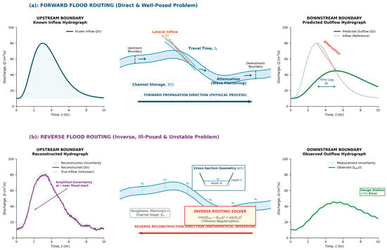
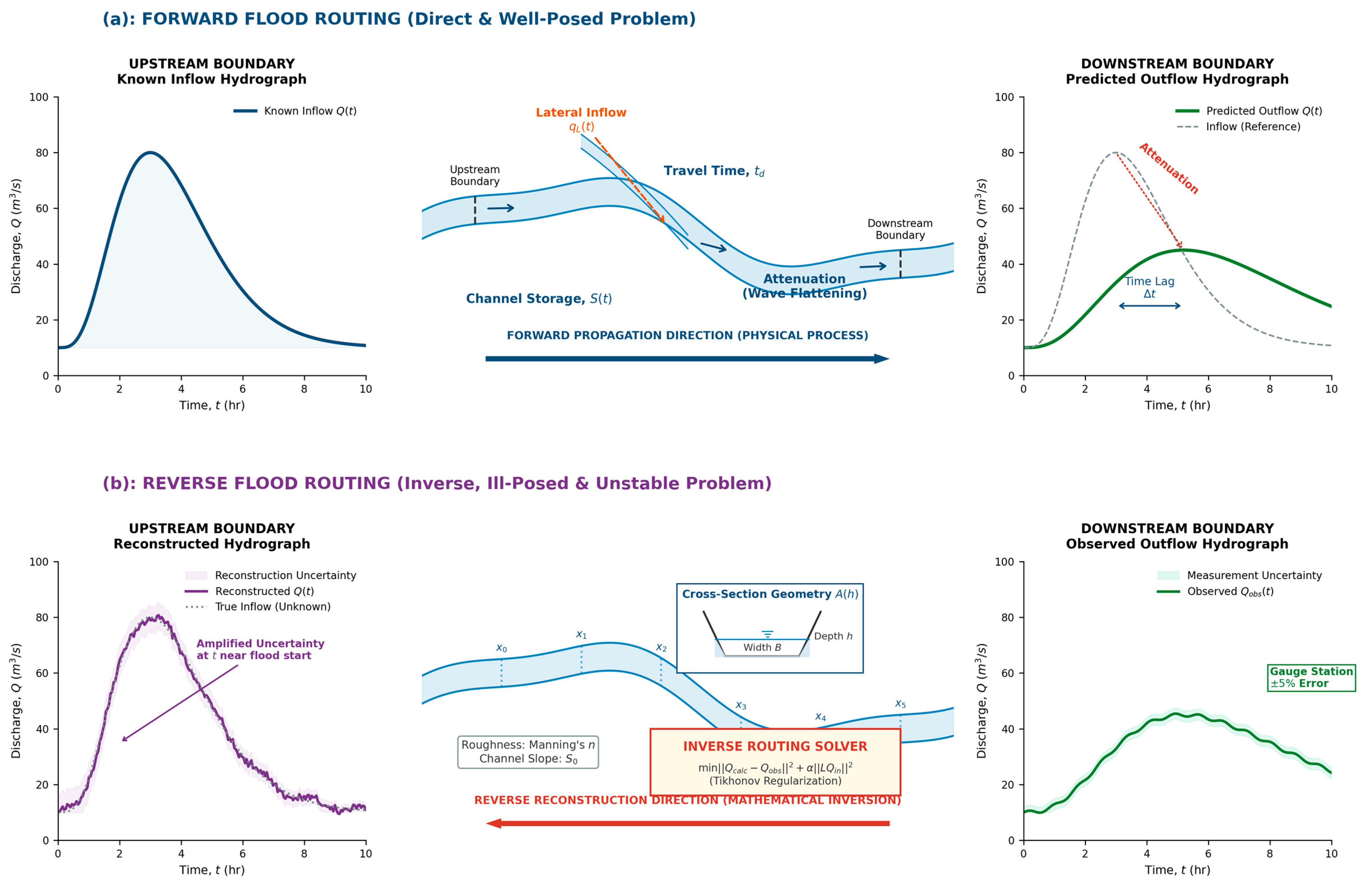
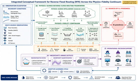
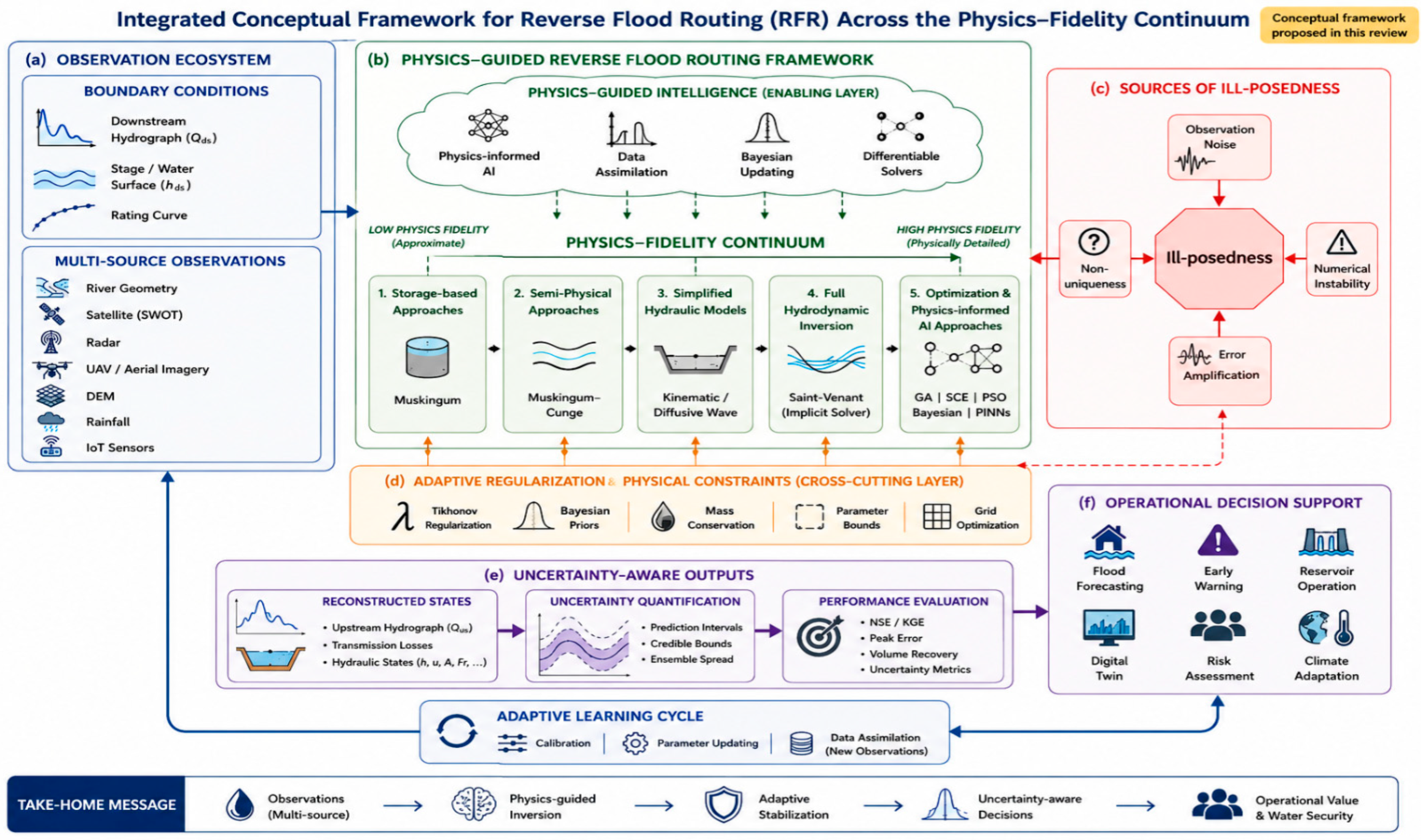
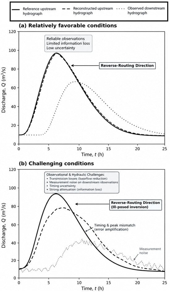
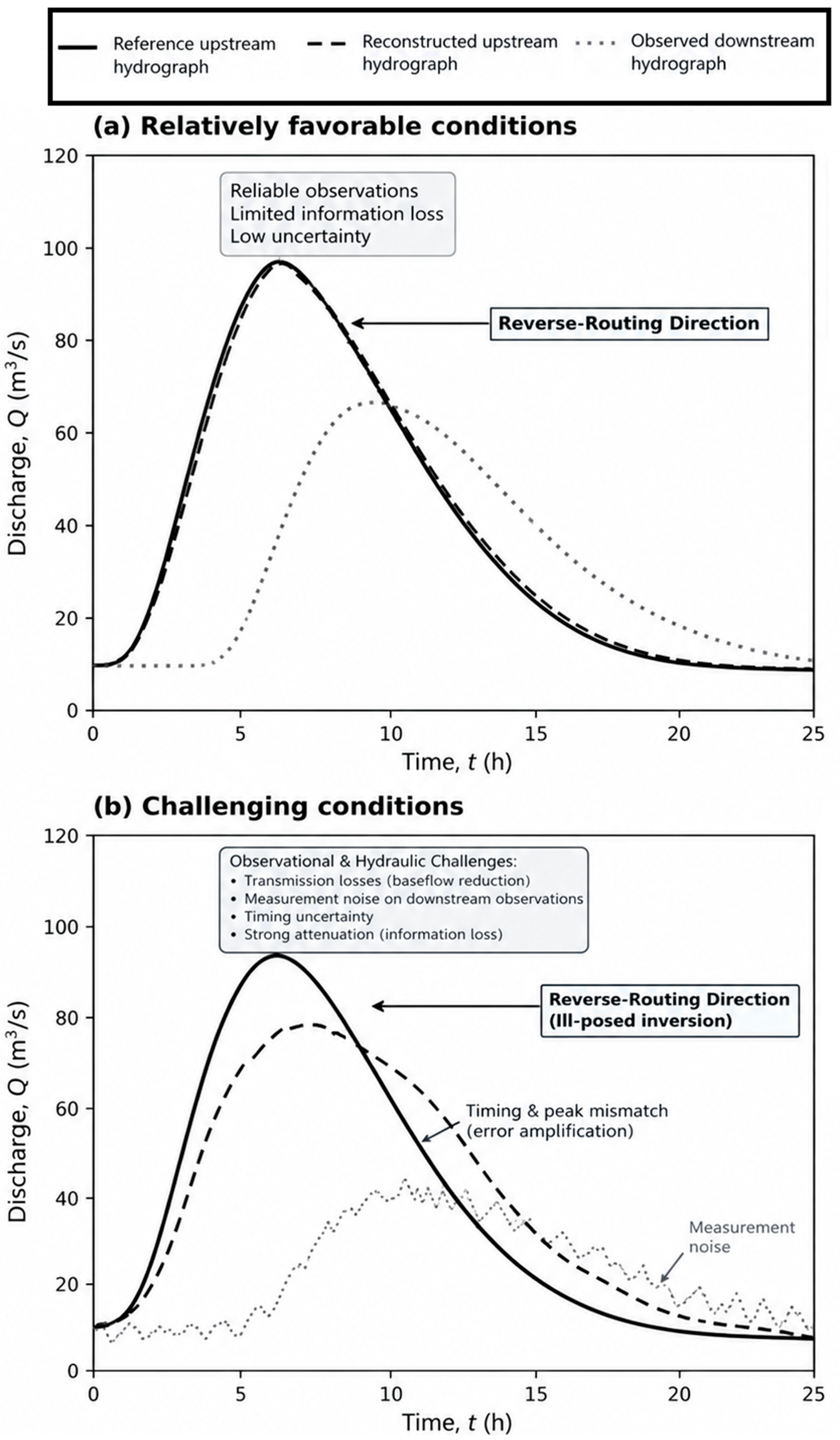

Disclaimer/Publisher’s Note: The statements, opinions and data contained in all publications are solely those of the individual author(s) and contributor(s) and not of MDPI and/or the editor(s). MDPI and/or the editor(s) disclaim responsibility for any injury to people or property resulting from any ideas, methods, instructions or products referred to in the content. |
© 2026 by the authors. Licensee MDPI, Basel, Switzerland. This article is an open access article distributed under the terms and conditions of the Creative Commons Attribution (CC BY) license.