Streamflow Estimation at Ungauged Sections in a Nested Basin Using an HEG-LSTM Model

Abstract

Streamflow estimation at ungauged sections is essential for flood warning, reservoir operation, water allocation, and basin management. Conventional regionalization approaches typically require the construction, calibration, and parameter transfer of conceptual or process-based hydrological models, resulting in high application costs when data are scarce, gauge networks are frequently adjusted, or management sections do not coincide with existing gauging stations. In recent years, regional Long Short-Term Memory (LSTM) networks have provided a data-driven alternative for ungauged streamflow estimation. However, existing studies have focused mainly on spatial generalization across independent catchments, with limited attention to hydrological information transfer among sections with different upstream and downstream relationships within the same nested basin. This study used five nested hydrological stations in the Fujiang River Basin to develop a Hydrological-Efficiency-Guided Long Short-Term Memory framework (HEG-LSTM) and compared it with a baseline LSTM. The model incorporated local meteorological forcing, antecedent precipitation, static basin attributes, and scenario-permitted donor-station discharge as inputs, and leave-one-station-out validation was adopted to assess cross-section applicability. To investigate the effects of different upstream and downstream relationships on streamflow estimation, three gauge-network scenarios were designed: S1 estimated downstream streamflow using upstream stations; S2 was downstream-to-upstream synchronous estimation; and S3 jointly estimated streamflow at an intermediate ungauged section using upstream and downstream stations. HEG-LSTM achieved a mean Nash–Sutcliffe efficiency (NSE) of 0.703, exceeding the 0.603 obtained by the baseline LSTM. The mean NSE values of HEG-LSTM under S1, S2, and S3 were 0.692, 0.695, and 0.730, respectively, with the best performance obtained under S3. Compared with the baseline LSTM, HEG-LSTM increased the coefficient of determination for high flow from 0.617 to 0.737 and that for annual peak flow from 0.731 to 0.770, whereas improvement in low flow correlation remained limited. Shapley Additive Explanations (SHAP) showed that donor-station discharge, drainage area, elevation, slope, and antecedent precipitation jointly influenced cross-section transferability. The proposed HEG-LSTM framework provides a methodological reference for streamflow estimation, historical streamflow estimation, and gauge-network optimization at ungauged sections in nested basins.

1. Introduction

Accurate streamflow information is fundamental to flood warning, reservoir operation, water allocation, environmental flow protection, and integrated basin management [1]. However, existing hydrological networks cannot cover every river section at which management, forecasting, or operational decisions are required [2]. In addition to completely ungauged catchments, data limitations commonly arise when records at newly established stations are too short, existing gauges are discontinued or interrupted for long periods, engineering works alter the hydrological representativeness of a section, or management sections do not coincide with gauging locations. Since the Prediction in Ungauged Basins (PUB) initiative, identifying transferable hydrological information in the absence of streamflow observations at a target section has become an important challenge in hydrology [3,4,5,6]. In river systems already covered by gauge networks, this challenge is not simply a matter of filling missing records; rather, it requires the use of available hydrometeorological information to estimate streamflow at ungauged or data-deficient sections.

Traditional PUB studies have primarily applied hydrological-model parameter regionalization. Conceptual or process-based hydrological models are first calibrated in gauged catchments, after which model parameters are transferred to ungauged catchments based on spatial proximity, catchment similarity, parameter regression, regional clustering, or machine-learning relationships [7]. For example, Merz, R. and Blöschl, G. [8] compared parameter regionalization methods for conceptual models across 308 Austrian catchments and showed that both spatial parameter variability and model structure influence regionalization outcomes. Oudin, L. et al. [9] systematically compared spatial proximity, physical similarity, and regression approaches across 913 French catchments and demonstrated that their performance is governed by hydroclimatic conditions and catchment characteristics. These methods retain explicit process representations and are suitable for scenario analysis and hydrological process interpretation. However, they usually require detailed topographic, soil, land-cover, and meteorological data, together with decisions on model structure, parameter calibration, and transfer rules. For arbitrary target sections within the same river network, individually constructing and regionalizing physical hydrological models may still involve substantial implementation costs [10].

Recent advances in large-sample hydrology and deep learning have provided new data-driven approaches to ungauged streamflow estimation. Long Short-Term Memory (LSTM) networks can learn nonlinear response, temporal dependence, and state-memory characteristics of rainfall–runoff processes from continuous meteorological forcing and streamflow sequences [11]. Regional LSTM further use joint training across multiple catchments to transfer shared model parameters and latent hydrological representations to target catchments that are excluded from training. Using the CAMELS dataset, Kratzert, F. et al. [12] showed that regional LSTM incorporating static catchment attributes can learn hydrological differences among catchments and achieve high accuracy in large-sample regional simulations. A comparison across 148 North American catchments by Arsenault, R. et al. [13] further demonstrated that regional LSTM models can outperform several conventional hydrological-model regionalization approaches for continuous streamflow simulation in ungauged catchments. Kratzert, F. et al. [14] subsequently emphasized that multi-basin training is essential for exploiting the spatial generalization capability of LSTM models. These studies show that data-driven models do not simply replace traditional hydrological models; rather, they can learn regional hydrological response relationships with transfer potential from information across multiple stations or catchments [15,16,17].

Despite rapid progress in regional deep learning, existing studies mostly treat catchments or stations as relatively independent sample units and focus on spatial generalization across different catchments. In nested sections within the same river network, upstream and downstream stations are connected by explicit hydrological pathways [18]. Upstream streamflow integrates antecedent precipitation, catchment storage, runoff generation, and routing processes, whereas downstream streamflow additionally incorporates intervening inflow, tributary contributions, channel propagation, and potential human influences. Consequently, the spatial position of donor stations relative to a target section and the direction of their information directly affect the physical interpretation and application scope of streamflow estimation. Recent studies involving spatially recursive LSTM, river-network routing models, and graph neural networks have highlighted the importance of river-network topology and flow-concentration processes in streamflow modeling [19,20]. Vaheddoost, B. et al. [21] estimated tributary discharge from precipitation and the direct-runoff/base-flow components at a selected mainstream reference station, and then evaluated the resulting flow-duration and mass-flow curves. Their work highlights that reference-station selection and hydrological decomposition can be important when the objective is to characterize flow-frequency and cumulative-water-availability features at ungauged tributaries. Nevertheless, systematic comparisons of the effects of upstream, downstream, and combined upstream and downstream information on streamflow estimation at ungauged sections within the same nested basin remain limited.

In addition to input configuration, the training objective also affects the ability of deep-learning models to represent different flow regimes. Conventional mean squared error mainly constrains pointwise differences between estimated and observed values, but its optimization direction may not fully align with hydrological evaluation requirements such as Nash–Sutcliffe efficiency (NSE), water-balance bias, low-flow errors, and peak-flow simulation. Previous studies have shown that the performance of regional LSTM is influenced by normalization strategies, loss-function design, and the weighting of high-flow and low-flow samples [12,22,23]. In particular, reliance on a single error function can lead to unbalanced fitting across different flow ranges when simulating high flows and extreme peaks. It is therefore necessary to construct a training objective that considers overall hydrological efficiency, flow-magnitude bias, and different flow regimes when evaluating its suitability for streamflow estimation at ungauged sections in nested basins.

Kratzert, F. et al. [15] used regional LSTM models with static attributes for large-sample cross-basin generalization, but did not use adjacent-section same-day discharge as scenario-controlled donor information. Arsenault, R. et al. [13] compared regional LSTM models with traditional regionalization across 148 North American catchments, but did not test information direction in one connected network. Yu, Q. et al. [19] incorporated spatially distributed information into LSTM models and showed the value of explicit spatial structure, but did not systematically compare upstream, downstream, and bidirectional donor sets while holding out the target section. Accordingly, this study develops a Hydrological-Efficiency-Guided Long Short-Term Memory (HEG-LSTM) framework for streamflow estimation using five nested hydrological stations in the Fujiang River Basin and compares it with a baseline LSTM. The study has three objectives. First, it evaluates the ability of HEG-LSTM to represent the overall hydrograph, high-flow and low-flow conditions, and annual peak flows. Second, to investigate the effects of section relationships along the upstream and downstream direction on streamflow estimation, three gauge-network scenarios are considered: S1 estimates downstream streamflow using upstream stations, S2 estimates streamflow at an ungauged upstream section using downstream stations, and S3 jointly estimates streamflow at an intermediate ungauged section using upstream and downstream stations. Third, Shapley Additive Explanations (SHAP) are used to analyze the relative contributions of donor-station discharge, meteorological forcing, and static basin attributes to model outputs. This study aims to provide a transferable data-driven approach for streamflow estimation at ungauged sections and for using gauge-network information in nested basins.

2. Study Area and Data

2.1. Study Area

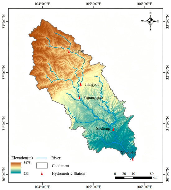
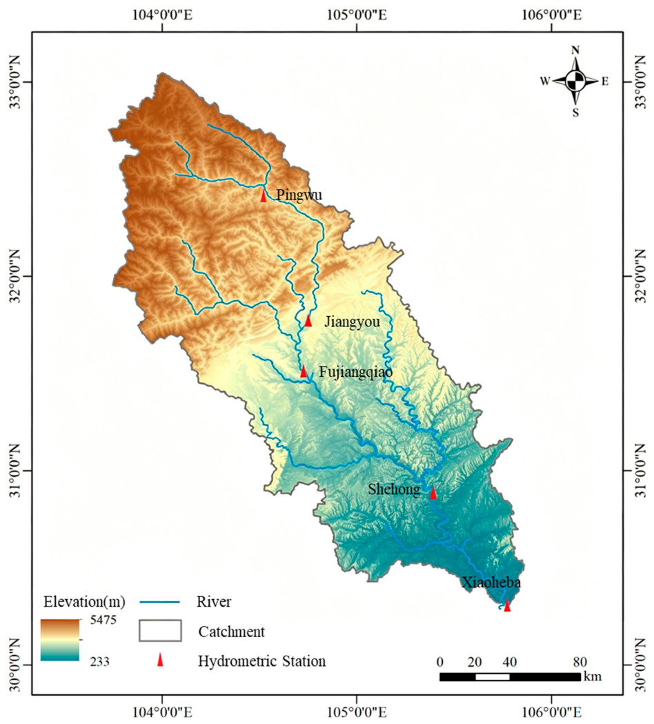
The Fujiang River is an important tributary of the Jialing River in the upper Yangtze River Basin. The study area transitions from high-relief mountain and gorge terrain in the northwest to hilly and plain landscapes in the southeast. Topographic relief, river-network structure, and monsoonal precipitation jointly control runoff generation, flow concentration, and channel propagation. Precipitation is unevenly distributed throughout the year and is concentrated during the flood season, resulting in pronounced seasonal and event-based streamflow responses. Five hydrological stations along the Fujiang River main stem, Pingwu, Jiangyou, Fujiangqiao, Shehong, and Xiaoheba, were selected to form a nested station network, with stations arranged sequentially from upstream to downstream (Figure 1).

Figure 1. Location of the Fujiang River Basin and the five hydrological stations.

Drainage area increases from 4424 km² to 29,114 km², mean elevation decreases from 2756 m to 1184 m, and mean slope decreases from 22.3° to 10.8°, reflecting a pronounced topographic gradient from mountainous headwaters to hilly and valley settings in the middle and lower reaches. The sections differ substantially in drainage area, topographic conditions, river distance, precipitation conditions, and streamflow processes, providing a representative setting for analyzing cross-section hydrological information transfer within a nested basin. Station attributes and data statistics are presented in Table 1.

Table 1. Basic information on the five hydrological stations.

Station	Area (km2)	Elevation (m)	Slope (°)	River Distance (km)	Mean P (mm d−1)	Mean Discharge (m3 s−1)	Peak Discharge (m3 s−1)
Pingwu	4424	2756	22.3	0.0	1.58	122	2470
Jiangyou	6052	2376	20.7	105.5	1.66	156	3130
Fujiangqiao	12,205	2074	19.8	142.3	1.33	296	10,100
Shehong	24,093	1348	12.4	269.9	1.42	444	17,763
Xiaoheba	29,114	1184	10.8	383.2	1.42	450	21,000

2.2. Dataset

Daily precipitation P (mm d⁻¹), evapotranspiration E (mm d⁻¹), mean temperature T_mean (°C), and streamflow Q (m³ s⁻¹) from 2008 to 2020 were used. Static basin attributes included drainage area, elevation, slope, and river distance. The data were provided by the Bureau of Hydrology, Changjiang Water Resources Commission. Model inputs were divided into three categories. The first category comprised meteorological variables, including same-day precipitation, evapotranspiration, and mean air temperature. To enhance the representation of catchment storage memory and antecedent rainfall conditions, antecedent precipitation accumulated over 3, 7, 15, and 30 days was additionally calculated from the daily precipitation series. These variables represent antecedent wetness at different temporal scales and provide information for identifying the lagged relationship between rainfall input and streamflow response. The second category comprised static attributes. To represent spatial differences among the basins controlled by different stations, drainage area, mean elevation, mean slope, and longitudinal river distance were selected as static basin attributes. Drainage area represents basin scale, mean elevation and slope represent topographic relief and potential runoff-generation and concentration conditions, and river distance describes the relative position of each station along the main stem. The third category comprised daily discharge from donor stations corresponding to each scenario. All data from the five stations were harmonized to the daily scale and matched using a consistent date sequence.

Daily precipitation, streamflow, and meteorological-station observations were supplied by the Bureau of Hydrology, Changjiang Water Resources Commission. The original minute-scale records were processed and interpolated to a common daily series covering 1 January 2008 to 31 December 2020 (4749 consecutive dates) without missing values. Antecedent precipitation was calculated as the sum over the preceding 3, 7, 15, or 30 calendar days, excluding the current day. Drainage area, mean elevation, mean slope, and related static attributes were calculated in GIS from catchment-boundary vector data and a 30-m DEM.

3. Methodology

3.1. Overall Framework

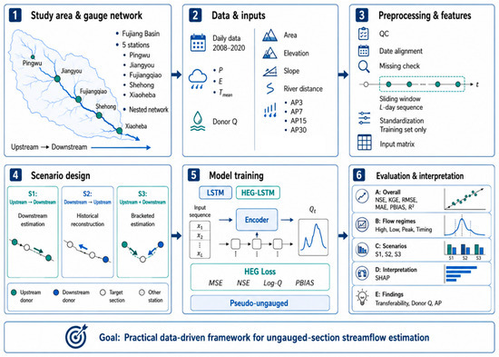
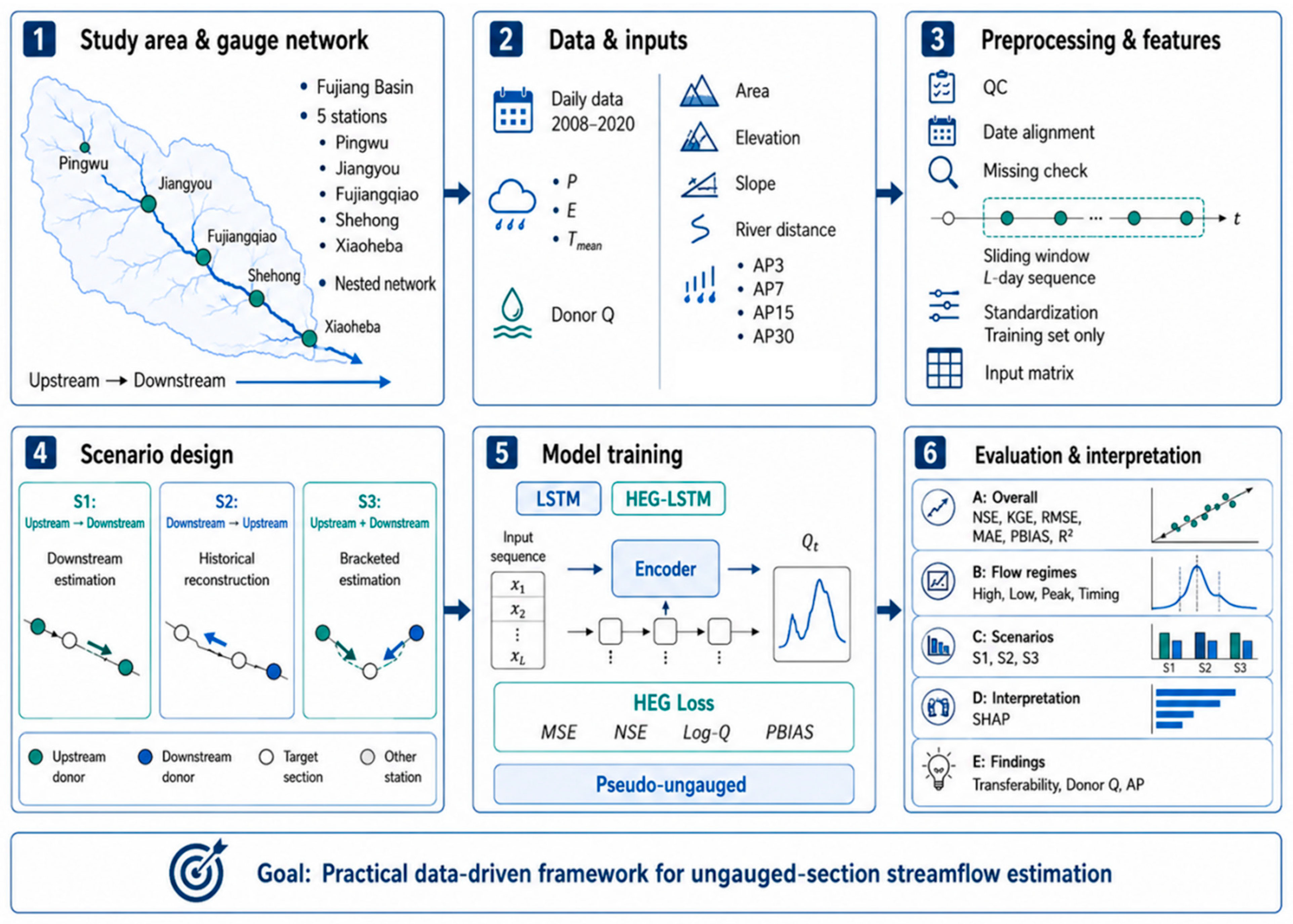
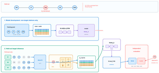
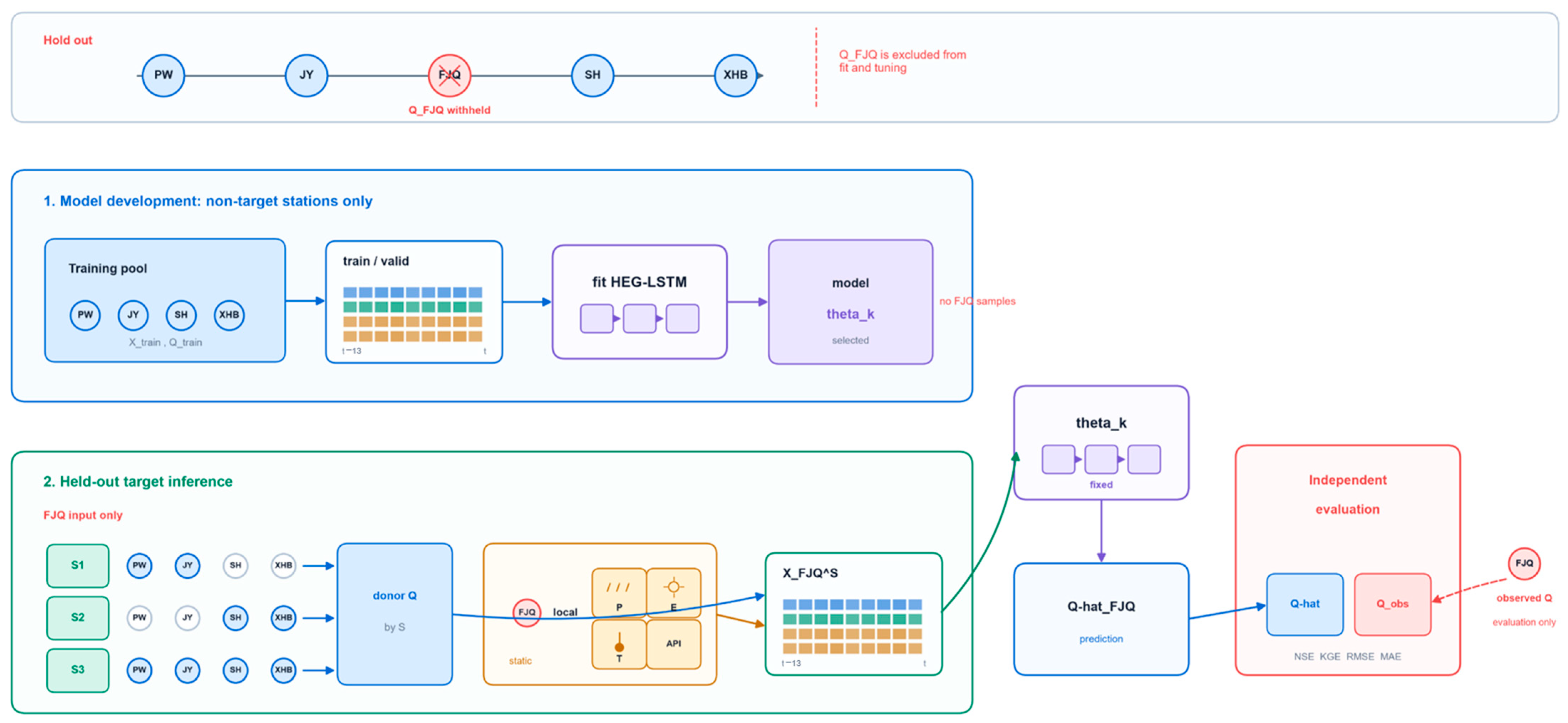
A regional streamflow-estimation framework was developed for ungauged sections in nested basins (Figure 2). For each station used in the model construction, local meteorological forcing, antecedent precipitation, and static basin attributes of that station were used as local inputs, while discharge information from donor stations was incorporated according to the gauge-network scenario. The model was jointly trained across multiple stations to learn shared relationships among meteorological forcing, basin attributes, cross-station hydrological connectivity, and streamflow response, and the learned regional mapping was then transferred to the held-out ungauged section [12,13,24,25]. For a sample at modeled section i and time t, the input vector is expressed as:

$$x_{i,t}^{\left(r\right)}=\left[m_{i,t},a_{i,t},s_i,q_{i,t}^{D^{\left(r\right)}}\right]$$

(1)

where r denotes the gauge-network scenario; m_i,t represents same-day meteorological variables at section i, including precipitation, evapotranspiration, and mean temperature; a_i,t represents antecedent precipitation variables at the same section; s_i represents static basin attributes at the section, including drainage area, mean elevation, mean slope, and longitudinal river distance; and $q_{i,t}^{D^{\left(r\right)}}$ represents discharge information from donor stations available under scenario r. Based on a sliding time window of length L, the model estimates streamflow at the modeled section as:

$${\widehat{Q}}_{i,t}=f_{\theta }\left(X_{i,t-L+1:t}^{\left(r\right)}\right)$$

(2)

Figure 2. Workflow of the streamflow-estimation framework for ungauged sections and the hydrological-efficiency-guided loss.

During regional training, i successively denotes the four gauged stations, and each station provides input samples constructed from its own meteorological variables and static attributes, with its corresponding observed streamflow serving as the supervisory target. During transfer, the held-out target section is represented using the same feature-construction procedure. Its meteorological variables, antecedent precipitation, and static attributes are combined with scenario-permitted donor-station discharge to form an input matrix with the same dimensionality as that used during training, and the trained model is then applied to generate streamflow estimates.

3.2. Scenario Design

Three gauge-network scenarios were developed to investigate the effects of different upstream and downstream relationships on streamflow estimation at ungauged sections. In each scenario, donor stations were selected according to their river-network positions relative to the target section. S1 represents downstream streamflow estimation using upstream stations. In this scenario, only discharge information from stations upstream of the target section, together with meteorological forcing at the target section, was used to estimate downstream streamflow. This scenario follows the direction of river flow propagation and can be used to examine how upstream hydrological information supports downstream streamflow estimation. Because this study used donor discharge aligned with the target section on the same day, S1 represents downstream streamflow estimation under temporally synchronous conditions. Application to real-time forecasting would require further consideration of channel travel time and data-transmission timeliness [20,26]. S2 represents streamflow estimation at an ungauged upstream section using downstream stations. In this scenario, only discharge information from stations downstream of the target section was used to estimate streamflow at the ungauged upstream section. Because downstream discharge includes integrated effects of intervening runoff, tributary inflow, and channel propagation, this scenario is primarily applicable to historical-process and estimation. S3 represents joint streamflow estimation at an intermediate ungauged section using upstream and downstream stations. In this scenario, discharge information from stations upstream and downstream of the target section was used together with local meteorological forcing and static attributes to estimate streamflow at the intermediate section (Figure 3). This scenario is applicable to data completion within a gauge network, historical streamflow estimation, and offline river-network analysis.

Figure 3. Workflow of the leave-one-station example (Fu Jiangqiao).

All donor-station discharge series were aligned to the target date; consequently, the three experiments represent synchronous estimation or reconstruction rather than forecasting with a positive lead time. S1 is same-day downstream estimation supported by upstream information; S2 is downstream-to-upstream synchronous estimation, primarily suitable for historical record estimation, consistency checks, and gap filling when downstream observations remain available; and S3 is same-day estimation/reconstruction of an intermediate section using both upstream and downstream information. For each target-section-scenario experiment, the target station is removed from the donor list before feature construction. The input tensor never contains the target-station discharge or any lagged target discharge. Each permitted donor station is represented by a separate one-dimensional feature; columns are date-aligned, their membership and order are fixed by the scenario, and a date is excluded before window construction if any required donor observation is unavailable.

3.3. The LSTM Model

LSTM is a recurrent neural-network architecture capable of representing long-term dependencies [27] and is suitable for describing nonlinear response, storage memory, and time-lag characteristics in rainfall–runoff processes [11]. For an input sequence x_t, the LSTM controls information updates in the memory cell through input, forget, and output gates, which can be expressed as:

$$i_t=\sigma \left(W_i{x}_t+U_i{h}_{t-1}+b_i\right)$$

(3)

$$f_t=\sigma \left(W_f{x}_t+U_f{h}_{t-1}+b_f\right)$$

(4)

$$o_t=\sigma \left(W_o{x}_t+U_o{h}_{t-1}+b_o\right)$$

(5)

$${\tilde{c}}_t=\tanh \left(W_c{x}_t+U_c{h}_{t-1}+b_c\right)$$

(6)

$$c_t=f_t\odot c_{t-1}+i_t\odot {\tilde{c}}_t$$

(7)

$$h_t=o_t\odot \tanh \left(c_t\right)$$

(8)

where i_t, f_t, and o_t denote the input, forget, and output gates, respectively; c_t denotes the memory-cell state; h_t denotes the hidden state; σ and tanh denote the sigmoid and hyperbolic tangent activation functions, respectively; and ⊙ denotes element-wise multiplication. Finally, the hidden state is mapped through a fully connected layer to the daily streamflow estimate at the target section:

$${\widehat{Q}}_t=W_y{h}_t+b_y$$

(9)

The baseline LSTM was trained using mean squared error and served as the benchmark model for HEG-LSTM. The two models used identical input variables, sequence length, network architecture, and training strategy, ensuring that performance differences primarily reflect the effect of loss-function design.

3.4. Hydrological-Efficiency-Guided LSTM Model

HEG-LSTM retains the network architecture of the baseline LSTM and introduces a hydrological-efficiency-guided composite loss so that model training simultaneously considers overall error, hydrological efficiency, errors across different flow ranges, and systematic water-balance bias. The loss function is defined as:

$$L_{HEG}=\alpha L_{MSE,s}+\beta \left(1-NSE\right)+\gamma L_{\log Q}+\delta PBIA{S}^2$$

(10)

$$L_{MSE,s}={\displaystyle \frac{1}{N}}{\displaystyle \sum _{t=1}^N{\left({\widehat{Q}}_{s,t}-Q_{s,t}\right)}^2}$$

(11)

$$L_{\log Q}={\displaystyle \frac{1}{N}}{\displaystyle \sum _{t=1}^N{\left[\log \left(1+\max \left({\widehat{Q}}_t,0\right)\right)-\log (1+\max (Q_t,0\left)\right)\right]}^2}$$

(12)

$$NSE=1-{\displaystyle \frac{{\displaystyle \sum _{t=1}^N{\left(Q_t-{\widehat{Q}}_t\right)}^2}}{{\displaystyle \sum _{t=1}^N{\left(Q_t-{\overline{Q}}_t\right)}^2}}}$$

(13)

$$PBIAS=100\times {\displaystyle \frac{{\displaystyle \sum _{t=1}^N\left({\widehat{Q}}_t-Q_t\right)}}{{\displaystyle \sum _{t=1}^N{Q}_t}}}$$

(14)

where Q_t and ${\widehat{Q}}_t$ denote observed and estimated streamflow, respectively; and $\overline{Q}$ denotes the mean observed streamflow. The loss weights α = 0.45 and β = 0.45 assign the main emphasis to stable overall hydrograph fitting and hydrological efficiency, whereas γ = 0.05 and δ = 0.05 retain the logarithmic-flow and PBIAS terms as lower-weight regularizers. In five fixed-weight experiments, the 0.45/0.45/0.05/0.05 setting was a well-balanced setting among those tested, not as a universally optimal weight combination. In this loss function, standardized mean squared error maintains stable overall fitting, the NSE term improves the representation of overall streamflow dynamics, the logarithmic-flow term enhances discrimination of low and medium flows, and the PBIAS term suppresses systematic water-balance bias. HEG-LSTM does not alter the input information or network architecture; instead, it uses joint multi-objective optimization to align model training more closely with hydrological evaluation requirements.

To evaluate the spatial transferability of the model under ungauged-section conditions, leave-one-station-out validation was adopted [13]. In each experiment, one hydrological station was selected as the target section, and all streamflow samples from that station were excluded from model training, validation, normalization-parameter estimation, and hyperparameter selection. Samples from the remaining four gauged stations formed the regional training dataset and were divided chronologically into training and validation sets. The complete available streamflow series at the held-out station was used only for final independent testing. During training, all dynamic variables and static attributes were standardized using statistics calculated from the training samples, and the same normalization parameters were applied to the validation set and the target-station test set. To preserve temporal structure, both sample partitioning and sliding-window construction followed chronological order, without random reshuffling of individual time-series samples. Early stopping was adopted, and the model parameters associated with the minimum validation loss were retained as the final model.

Both LSTM and HEG-LSTM used the same 14-d input sequence, two LSTM layers, 96 hidden units per layer, a dropout rate of 0.15, the Adam optimizer, a learning rate of 7 × 10⁻⁴, a batch size of 64, a maximum of 120 epochs, early stopping with a patience of 14 epochs, and a random seed of 42 for the archived main results. Hyperparameters were selected by manual trials using the same chronological data split for both models; the final comparison therefore differs only in the loss function.

3.5. Evaluation Metrics and Interpretability Analysis

Model performance was comprehensively evaluated using NSE, Kling–Gupta efficiency (KGE), root mean square error (RMSE), mean absolute error (MAE), percent bias, and the coefficient of determination. KGE, RMSE, and MAE are defined as:

$$KGE=1-\sqrt{{\left(r-1\right)}^2+{\left({\alpha }_{\sigma }-1\right)}^2+{\left({\beta }_{\mu }-1\right)}^2}$$

(15)

$$RMSE=\sqrt{{\displaystyle \frac{1}{N}}{\displaystyle \sum _{t=1}^N{\left({\widehat{Q}}_t-Q_t\right)}^2}}$$

(16)

$$MAE={\displaystyle \frac{1}{N}}{\displaystyle \sum _{t=1}^N\left|{\widehat{Q}}_t-Q_t\right|}$$

(17)

where r is the Pearson correlation coefficient between observed and estimated values, α_σ is the ratio of standard deviations, and β_μ is the ratio of means. To assess the representation of different flow regimes, observations above the 75th percentile during the test period were defined as high-flow samples, whereas observations below the 25th percentile were defined as low-flow samples. RMSE, MAE, and the coefficient of determination were calculated separately for high-flow and low-flow conditions. Annual peak-flow performance was evaluated using the relative error, absolute relative error, coefficient of determination for annual peak flow, and peak-timing error [28].

To interpret feature contributions in HEG-LSTM, SHAP were used to quantify the marginal contribution of each input variable to model outputs [29]. For the nth sample, time step l, and feature j, let ϕ_n,l,j denote the SHAP value. The global importance of feature j is defined as:

$$I_j={\displaystyle \frac{1}{NL}}{\displaystyle \sum _{n=1}^N{\displaystyle \sum _{l=1}^L\left|{\varphi }_{n,l,j}\right|}}$$

(18)

4. Results and Discussion

4.1. Overall Model Performance

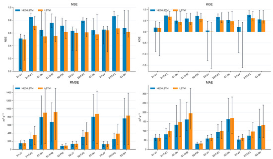
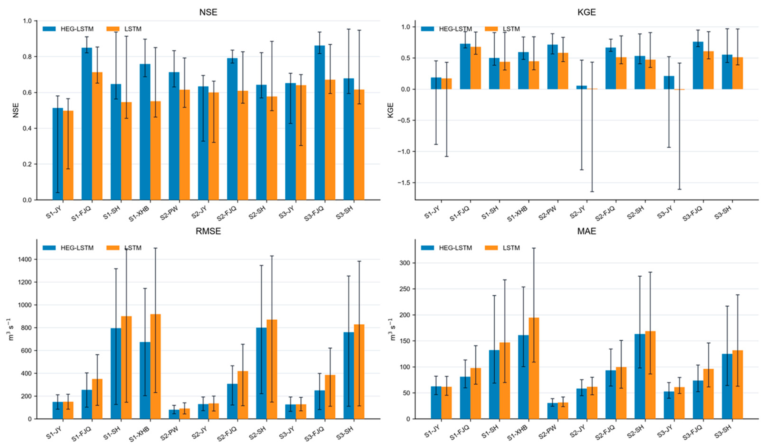
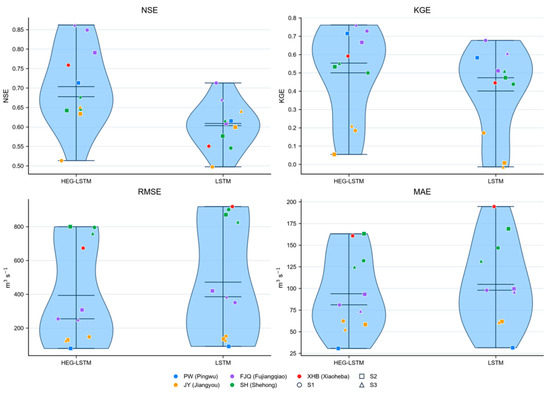
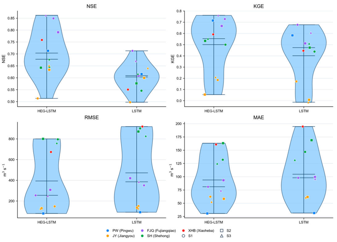
As shown in Table 2, Figure 4 and Figure 5, HEG-LSTM exhibited better overall streamflow-estimation performance across all test scenarios. The mean NSE of HEG-LSTM was 0.703, compared with 0.603 for the baseline LSTM, and the mean KGE increased from 0.401 to 0.500. Overall performance is defined as the unweighted arithmetic mean of the 11 target-section-scenario metrics. As robustness checks, HEG-LSTM NSE was 0.7034 for the scenario mean, 0.7120 for the station-equal mean, and 0.7203 for pooled daily estimations; the corresponding LSTM values were 0.6031, 0.5977, and 0.6087. Meanwhile, the mean RMSE and MAE of HEG-LSTM were 392.99 m³ s⁻¹ and 93.90 m³ s⁻¹, respectively, representing reductions of 78.02 m³ s⁻¹ and 10.76 m³ s⁻¹ relative to the baseline LSTM. To avoid scale dominance by larger downstream sections, NRMSE was defined as RMSE divided by the mean observed discharge for each target section, NMAE was defined analogously as MAE divided by mean observed discharge, and runoff-depth errors were calculated from the discharge and drainage area before averaging the 11 experiments. HEG-LSTM reduced NRMSE from 1.7775 to 1.5835, NMAE from 0.5782 to 0.5333, runoff-depth RMSE from 2.541 to 2.137 mm d⁻¹, and runoff-depth MAE from 0.682 to 0.619 mm d⁻¹. Overall, PBIAS decreased from 14.55% to 12.97%, indicating that HEG-LSTM also provided an advantage in controlling the aggregate water-balance bias. Expressed relative to the baseline LSTM, HEG-LSTM reduced the aggregate RMSE by 16.6% and the aggregate MAE by 10.3%. By contrast, the decrease in PBIAS was modest, with an absolute reduction of 1.58 percentage points. This difference indicates that the principal benefit of the hydrological-efficiency-guided loss was not a uniform reduction in every error component, but a more favorable balance between hydrograph dynamics and pointwise error magnitude. In particular, the concurrent increase in NSE and KGE suggests that the improved performance was associated with both more accurate temporal variation and a better representation of the mean and variability components of streamflow.

Table 2. Scenario-specific performance summary of LSTM and HEG-LSTM.

Group	Model	NSE	KGE	RMSE	MAE	PBIAS
Overall	HEG-LSTM	0.703	0.500	392.99	93.90	12.97
Overall	LSTM	0.603	0.401	471.01	104.66	14.55
S1	HEG-LSTM	0.692	0.501	467.85	109.06	7.00
S1	LSTM	0.577	0.433	580.37	125.28	6.44
S2	HEG-LSTM	0.695	0.492	328.96	86.32	14.60
S2	LSTM	0.600	0.393	379.27	90.39	14.21
S3	HEG-LSTM	0.730	0.508	378.55	83.78	18.75
S3	LSTM	0.642	0.368	447.51	96.19	25.81

Figure 4. Comparison of NSE, KGE, RMSE, and MAE between LSTM and HEG-LSTM.

Figure 5. Distributions of test-period performance metrics for the two models.

To quantify initialization variability, each archived configuration was additionally trained with random seeds 7, 42, and 2026 under the same 11 target-section-scenario experiments. The corresponding mean NSE values were 0.7094, 0.7034, and 0.6555 for HEG-LSTM (standard deviation 0.0295) and 0.6034, 0.6031, and 0.6106 for LSTM (standard deviation 0.0042). We tested input-window lengths of L = 7, 14, 30, and 60 d while holding the network structure, loss weights, training budget, data split, and random seed fixed. Their mean NSE values were 0.7043, 0.7034, 0.7017, and 0.6798, respectively. Although L = 14 did not give the numerically highest mean NSE, it retained short- to medium-term hydrological memory while avoiding the performance decrease and additional computational burden observed for L = 60; it is therefore used as a parsimonious and stable choice. For the 11 matched target-section-scenario experiments, the mean paired NSE difference between HEG-LSTM and LSTM was 0.1003. An exact Wilcoxon signed-rank test gave p = 0.00098, and a 10,000-resample scenario bootstrap produced a 95% confidence interval of 0.0616–0.1402. A 30-d moving-block bootstrap applied to paired daily estimations gave a corresponding interval of 0.0573–0.1128.

The distributions of the performance metrics further show that the advantage of HEG-LSTM was not limited to mean values. Compared with the baseline LSTM, the distributions of NSE and KGE for HEG-LSTM shifted towards better ranges, whereas the upper ranges of RMSE and MAE decreased markedly. This indicates that the hydrological-efficiency-guided loss reduced the influence of large-error events in most test combinations. However, the improvement in PBIAS was not consistent across all scenarios. For example, PBIAS values for HEG-LSTM under S1 and S2 were 7.00% and 14.60%, respectively, which were slightly higher than those of the baseline LSTM at 6.44% and 14.21%. A clearer improvement in water-balance bias was observed only under S3. Therefore, the main advantage of HEG-LSTM should be summarized as improved overall hydrograph fitting and error control rather than unconditional superiority for every hydrological metric.

These results indicate that a training objective that jointly considers standardized error, overall hydrological efficiency, logarithmic-flow error, and water-balance bias can alleviate the limitations of a single mean squared error objective in representing different flow processes. In particular, in multi-station modeling for nested basins, the composite loss allows the model to better balance streamflow dynamics and error magnitude. Nevertheless, the magnitude of improvement under different gauge-network information conditions remains influenced by donor information, target-section location, and the complexity of streamflow processes. Although the two models still exhibit overlapping performance ranges, HEG-LSTM shows a systematic shift towards higher NSE and KGE values and lower RMSE and MAE values. Such overlap is expected because the difficulty of cross-section estimation varies among stations and scenarios. Therefore, the improvement should be interpreted as a robust average advantage across multiple station combinations rather than as evidence that the proposed loss function is optimal for every hydrological condition. This finding is consistent with previous studies showing that the choice of training objective can alter the balance among hydrograph accuracy, water-balance bias, and flow-regime-specific performance [30,31,32,33].

The comparison with previous LSTM studies should be interpreted at the level of modeling strategy rather than as a direct numerical ranking across datasets. Conventional rainfall–runoff LSTM studies often optimize one primary objective and then evaluate several hydrological metrics after training, whereas this HEG-LSTM retains the same inputs, network architecture, chronological split, and output setting as the baseline LSTM and changes only the training objective. In contrast, hybrid approaches, such as that proposed by Cho, K. and Kim, Y. [34], improve streamflow prediction by coupling an LSTM with a physically based WRF-Hydro model; they therefore introduce a different source of hydrological information and are not directly comparable with this loss-function modification. The non-uniform changes in NSE, KGE, RMSE, MAE, and PBIAS are consequently expected: these metrics emphasize different aspects of hydrograph behavior and may create competing optimization preferences [32,33]. The contribution of HEG-LSTM is therefore framed as a better balance between overall hydrograph fitting and error control in the tested nested-station setting, rather than unconditional superiority for every metric or scenario.

4.2. Effects of Upstream and Downstream Station Relationships

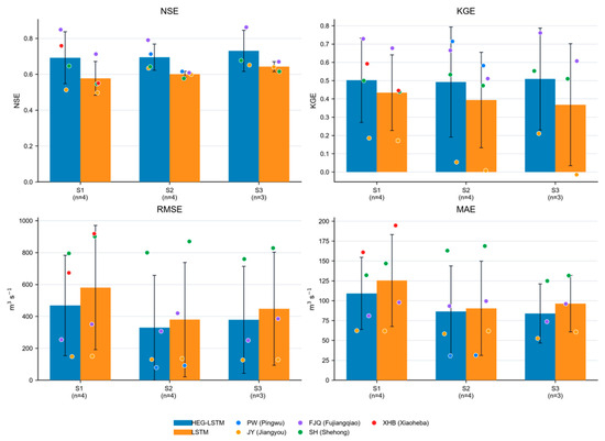
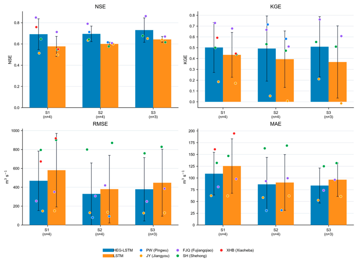
The results under different gauge-network scenarios shown in Figure 6 indicate that the relative relationships between upstream and downstream stations and the target section substantially affect streamflow estimation. Under S1, HEG-LSTM achieved mean NSE, KGE, and RMSE values of 0.692, 0.501, and 467.85 m³ s⁻¹, respectively, outperforming the baseline LSTM values of 0.577, 0.433, and 580.37 m³ s⁻¹. The increase in NSE reached 0.115, indicating that streamflow at upstream stations provides effective information for representing flow variations at downstream sections. Under S2, the mean NSE of HEG-LSTM was 0.695, higher than the 0.600 obtained by the baseline LSTM, whereas mean RMSE decreased from 379.27 m³ s⁻¹ to 328.96 m³ s⁻¹. S2 produced the lowest RMSE among the three scenarios, indicating that downstream discharge contains integrated hydrological information related to upstream streamflow variations. However, downstream discharge is also influenced by intervening runoff generation, tributary inflow, and channel propagation. Therefore, the higher accuracy of this scenario primarily reflects its suitability for historical-process estimation and should not be interpreted directly as real-time estimation capability for upstream streamflow. Under S3, mean NSE and KGE reached 0.730 and 0.508, respectively, the highest values among the three scenarios, while mean RMSE was 378.55 m³ s⁻¹. The combined use of upstream and downstream station information provided more complete hydrological constraints for intermediate ungauged sections, allowing the model to use both upstream inflow states and downstream integrated response information. Notably, S3 was not optimal for every metric: RMSE and MAE under S2 were both lower than those under S3, showing that the relative advantages of the scenarios are not fully consistent across evaluation metrics.

Figure 6. Mean performance of the models under the S1, S2, and S3 scenarios.

The magnitude of improvement relative to the baseline model also differed among scenarios. HEG-LSTM reduced RMSE by 19.4%, 13.3%, and 15.4% under S1, S2, and S3, respectively. The largest relative reduction occurred under S1, indicating that the hydrological-efficiency-guided loss was particularly effective when upstream discharge information was used to estimate downstream flow. Nevertheless, S3 achieved the highest absolute NSE and KGE values, whereas S2 yielded the lowest RMSE and MAE. These contrasting results demonstrate that no single scenario was uniformly optimal across all metrics. Instead, the preferred configuration depends on whether the intended application prioritizes overall hydrograph similarity, absolute error reduction, historical estimation, or information completeness within the river network.

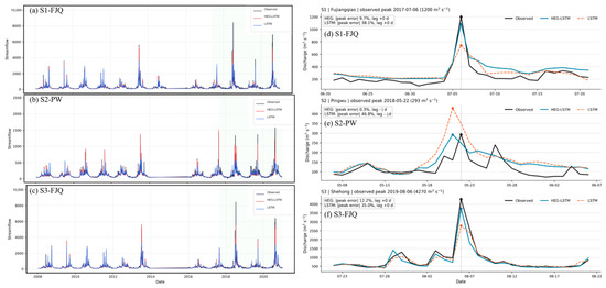
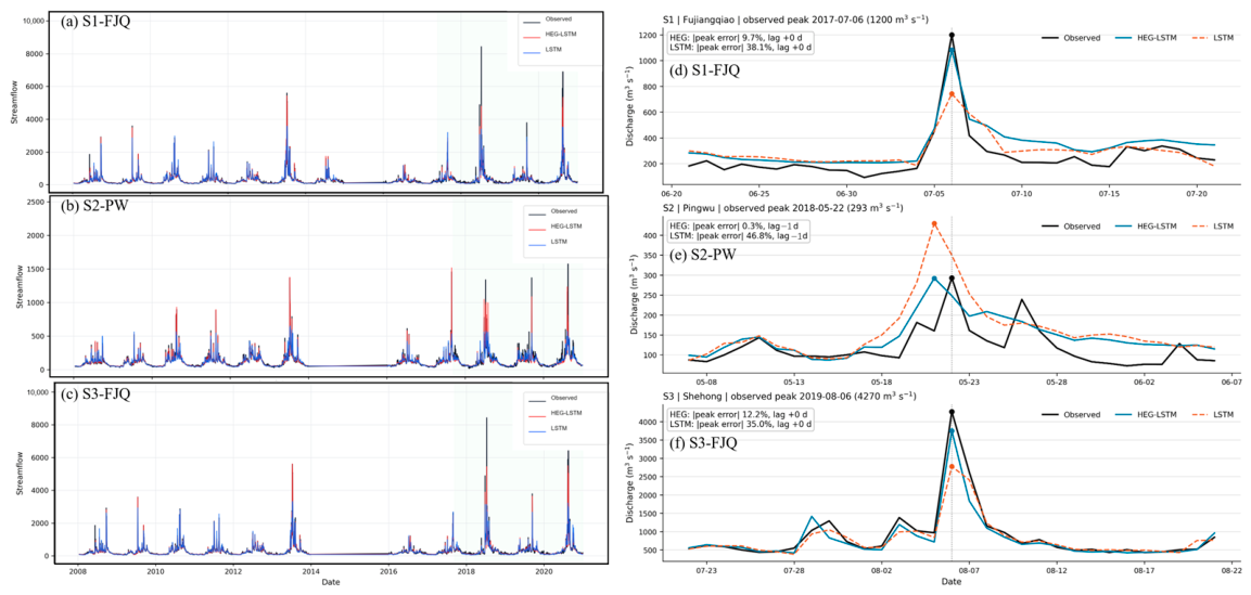
The representative hydrographs in Figure 7 show that HEG-LSTM reproduced seasonal streamflow variation and most medium-magnitude flood events reasonably well, but underestimated several extreme peaks to varying degrees. Across the three representative cases, HEG-LSTM generally reproduces the seasonal streamflow envelope and captures the timing of most moderate runoff events. However, the largest flood peaks remain smoother than the observations and are frequently underestimated. This pattern suggests that donor-station discharge provides valuable information on basin-scale hydrological state, but that local runoff generation, event-specific routing, and potentially unrepresented human disturbances still limit the estimation of rare extreme events. Similar limitations have been reported in spatially distributed and routing-aware deep learning studies, where explicitly representing river-network connectivity can improve streamflow estimation but does not eliminate uncertainty associated with local hydrological processes [18,19,35].

Figure 7. Representative observed and estimated streamflow hydrographs under the S1, S2, and S3 scenarios.

It is important to note that the evidence is limited to five stations within one nested basin and does not demonstrate cross-basin generalization. Spatial transferability refers here to the use of information from other stations for a held-out target section, whereas temporal generalization refers to performance in later periods for a fixed target-section-scenario setting. Validation across multiple climates, basin sizes, river-network topologies, data densities, and regulated rivers is required before broader transferability claims can be made. This study evaluates cross-section, date-aligned streamflow estimation within one nested station network. The chronological split prevents temporal leakage, but this evidence is not used to claim an independent temporal-generalization capability or cross-basin transferability. The use of donor discharge is related to, but distinct from, recent data-integration and river-network learning studies. Feng, D. et al. [17] showed that integrating heterogeneous information can improve LSTM-based streamflow prediction at continental scales, while spatially distributed LSTM and graph-based studies explicitly represent spatial relations or river-network connectivity [19,35]. Similarly, this model uses information from hydrologically connected sections rather than treating all stations as independent samples. However, this study is restricted to five nested stations in one basin and represents connectivity through scenario-permitted same-day donor discharge, not through an explicit routing equation, travel-time feature, or graph message-passing operation. Accordingly, the apparent benefit of S3 indicates that combined upstream and downstream observations provide complementary constraints in the tested intermediate-station combinations; it does not establish a general advantage of a particular topology model. For the same reason, S2 is interpreted as synchronous estimation or historical-process reconstruction, not as an upstream real-time forecast with lead time.

4.3. Model Performance Across Different Flow Regimes and Target Sections

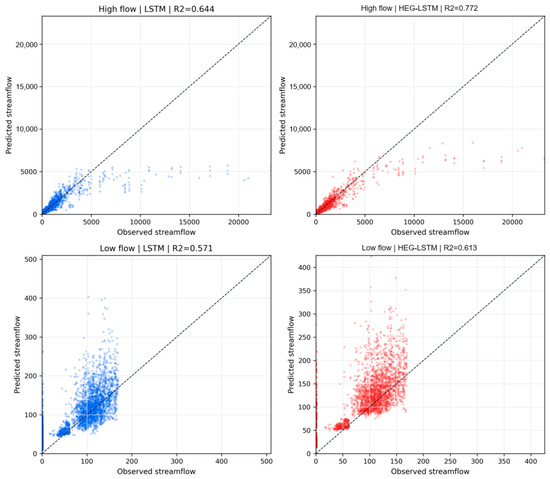
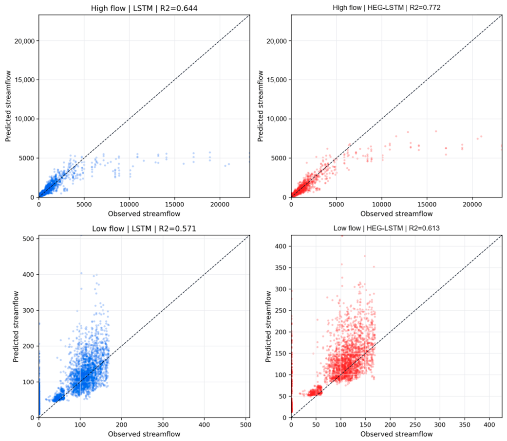
HEG-LSTM showed the most pronounced improvement for high-flow processes. As shown in Table 3 and Figure 8, the overall R² for high-flow conditions increased from 0.617 for the baseline LSTM to 0.737 for HEG-LSTM, whereas high-flow RMSE decreased from 931.88 m³ s⁻¹ to 775.09 m³ s⁻¹. Across all three scenarios, HEG-LSTM achieved higher high-flow R² values and lower high-flow RMSE and MAE values than the baseline LSTM. These results indicate that the hydrological-efficiency-guided loss improves the response of the model to flood-magnitude variations and, in particular, helps reduce the smoothing and underestimation of larger flows by the baseline LSTM. The improvement in high-flow performance was consistent across the three scenarios. Relative to the baseline LSTM, high-flow RMSE decreased by 19.7% under S1, 13.6% under S2, and 15.6% under S3. High-flow R² increased by 0.149, 0.111, and 0.091 under S1, S2, and S3, respectively. This consistency indicates that the composite loss did not improve high flows only under a specific station configuration, but enhanced the model response to large discharge events across contrasting information settings. The result is particularly relevant for nested river networks, where high-flow conditions are strongly influenced by the integration of upstream runoff, catchment wetness, and channel propagation.

Table 3. High-flow and low-flow performance summary by scenario.

Group	Model	High Flow			Low Flow
		R2	RMSE	MAE	R2	RMSE	MAE
S1	HEG-LSTM	0.758	923.08	292.73	0.057	45.37	30.99
S1	LSTM	0.609	1149.32	350.68	0.065	45.39	31.48
S2	HEG-LSTM	0.692	648.28	230.10	0.061	46.24	33.45
S2	LSTM	0.581	749.91	243.69	0.076	41.50	32.24
S3	HEG-LSTM	0.768	746.84	215.93	0.049	43.78	31.94
S3	LSTM	0.677	884.58	250.56	0.053	43.21	33.33

Figure 8. Comparison of high-flow and low-flow performance between LSTM and HEG-LSTM.

In contrast, the advantage of HEG-LSTM for low-flow processes was not stable. Overall, low-flow R² decreased slightly from 0.066 to 0.056, whereas low-flow MAE decreased only marginally from 32.26 m³ s⁻¹ to 32.14 m³ s⁻¹. Scenario-specific results show that low-flow MAE decreased slightly under S1 and S3, but low-flow RMSE and MAE under S2 were both higher for HEG-LSTM than for the baseline LSTM. This indicates that, although this composite loss includes a logarithmic-flow term, it remains insufficient to substantially improve the correlation and stability of low-flow processes. Low-flow variation may be influenced by groundwater recharge, local regulation, human water abstraction, and measurement error, none of which are explicitly represented in the current input variables. However, the low-flow results reveal a limitation shared by both models. Low-flow R² values remained close to zero under all scenarios, ranging from 0.049 to 0.076. Although HEG-LSTM slightly reduced low-flow MAE under S1 and S3, it did not improve low-flow correlation and performed less favorably than the baseline under S2. This result suggests that the logarithmic-flow term alone was insufficient to resolve the processes governing low-flow variability. In nested basins, low-flow conditions may depend on groundwater contribution, small-scale abstractions, reservoir regulation, delayed tributary inflow, and local channel storage, which are not explicitly represented by this set. Future improvements may therefore require hydrologically targeted low-flow inputs or a dedicated low-flow loss component rather than further adjustment of the existing general loss function [36,37].

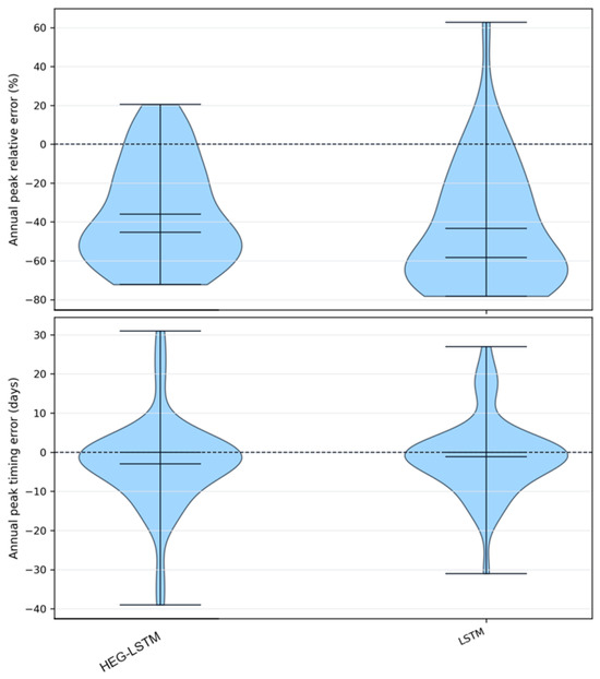
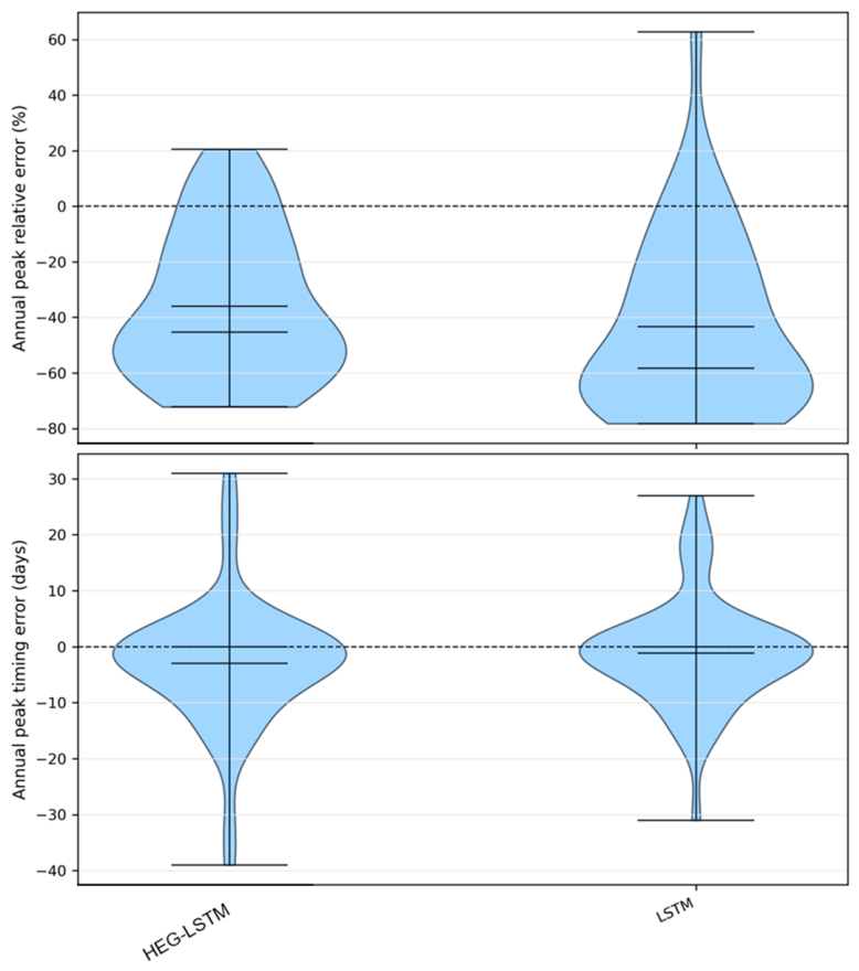
The annual peak-flow evaluation in Figure 9 further indicates that HEG-LSTM mainly improved peak-magnitude estimation. The overall annual peak-flow R² increased from 0.731 to 0.770, and mean absolute annual peak relative error decreased from 47.6% to 38.8%. However, the mean absolute peak-timing error of HEG-LSTM was 6.7 d, higher than the 5.9 d obtained by the baseline LSTM, showing that estimation of peak occurrence time did not improve simultaneously. In particular, under S2, the mean absolute peak-timing error of HEG-LSTM reached 9.1 d, compared with 5.2 d for the baseline LSTM. Under S3, peak-flow R² also decreased from 0.757 for the baseline LSTM to 0.695 for HEG-LSTM.

Figure 9. Distributions of annual peak-flow relative errors and peak-timing errors.

This framework should not be used alone for ecological-flow compliance, drought triggering, or precise flood-arrival warning. For the lowest 10% of flows, mean R² was 0.0223 for HEG-LSTM and 0.0227 for LSTM. For annual peaks, HEG-LSTM reduced mean absolute magnitude error from 47.6% to 38.8%, but its mean timing error was 6.7 d versus 5.9 d for LSTM. The method is thus best treated as an estimation or decision-support tool alongside independent operational checks. Therefore, the improvement of HEG-LSTM for annual peak flow is mainly reflected in peak magnitude rather than peak timing. This loss function does not directly impose a constraint on peak timing, and the model does not explicitly represent channel travel time, timing differences in local runoff generation and concentration, or reservoir operation. These limitations may restrict its ability to represent peak-arrival time. Future research could consider event-scale timing-error terms, travel-time features, or specialized training strategies for peak-flow processes. HEG-LSTM reduced mean absolute peak relative error and increased annual peak-flow R², but did not improve peak-timing accuracy. This divergence implies that the model learned useful information about the overall magnitude of flood events while remaining less capable of reproducing the exact temporal alignment of individual peaks. Such behavior is plausible when the input structure does not explicitly encode travel time, tributary arrival time, or operational regulation. Future work could therefore evaluate event-based loss functions that separately penalize peak magnitude and peak timing errors, particularly for applications in which flood warning lead time is more important than average hydrograph accuracy [30,38,39,40].

Performance differed substantially among target sections. HEG-LSTM achieved the highest mean NSE at Fujiangqiao, reaching 0.834, whereas the lowest mean NSE was observed at Jiangyou, at 0.599. This contrast indicates that the difficulty of streamflow estimation within nested basins is not determined solely by spatial distance between stations; it is also associated with the river-network position of the target section, available donor-station combinations, intervening-flow characteristics, and local hydrological processes.

Fujiangqiao is located in the middle part of the study area, and its streamflow can be constrained by both upstream inflow and downstream gauge-network information. It therefore showed relatively stable estimation performance across scenarios. In contrast, the larger estimation errors at Jiangyou suggest that its streamflow variation may be more strongly affected by local runoff generation, intervening inflow, or human influences that were not explicitly represented. Because this study did not directly include reservoir operation, water abstraction, tributary engineering, or channel-section changes, these factors can only be regarded as plausible explanations and cannot support definitive causal inference.

The station-specific results should therefore be interpreted as conditional on the available donor information rather than as a fixed ranking of hydrological complexity among stations. Fujiangqiao benefited from its intermediate position in the nested network, whereas the lower performance at Jiangyou may reflect a less favorable combination of upstream and downstream information, local inflow heterogeneity, and unresolved human influences. This interpretation is consistent with regional deep-learning studies showing that static attributes and spatial information can improve transferability, but cannot fully compensate for unobserved controls or differences in local hydrological processes [22,41,42]. Consequently, the performance of a target section should be evaluated together with its river-network setting rather than solely by its geographic distance from available donor stations. The performance differences among stations further indicate that cross-section streamflow estimation in nested river networks needs to consider river-network topology, basin attributes, and dynamic hydrological connectivity simultaneously. Estimation relationships based only on the nearest station or on a single donor station may not fully represent the actual hydrological response of different sections.

Previous deep-learning studies have shown that useful information can be extracted for high flows and extreme events, but that event representation remains sensitive to the information available to the model and to the intended use of the output [23,30]. Our result is consistent with this general pattern only in a limited sense. HEG-LSTM reduced high-flow errors and annual peak-magnitude error relative to the baseline LSTM, but the peak-timing error did not improve simultaneously. This difference is hydrologically plausible because the inputs used in this study contain donor discharge and local meteorological information but do not explicitly encode channel travel time, tributary arrival time, reservoir operation, or localized runoff concentration. This improvement should therefore be interpreted as improved estimation of flood magnitude within the tested synchronous data setting, rather than evidence that the model can provide precise peak-arrival warnings. The persistent weak low-flow correlation further indicates that groundwater exchange, small-scale abstractions, and other slowly varying controls are not sufficiently represented by the current predictors.

4.4. Feature Importance Analysis

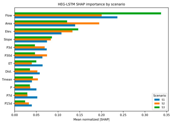
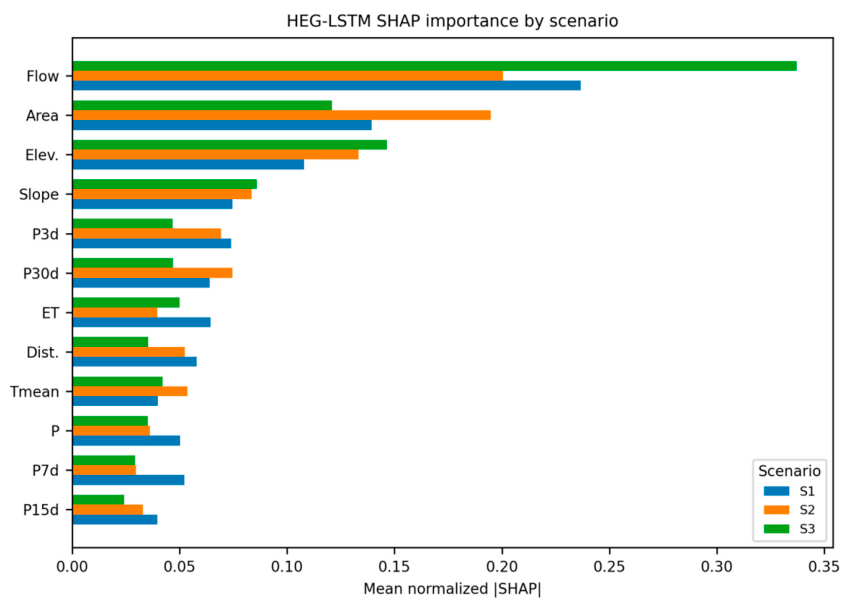
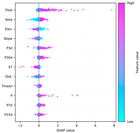
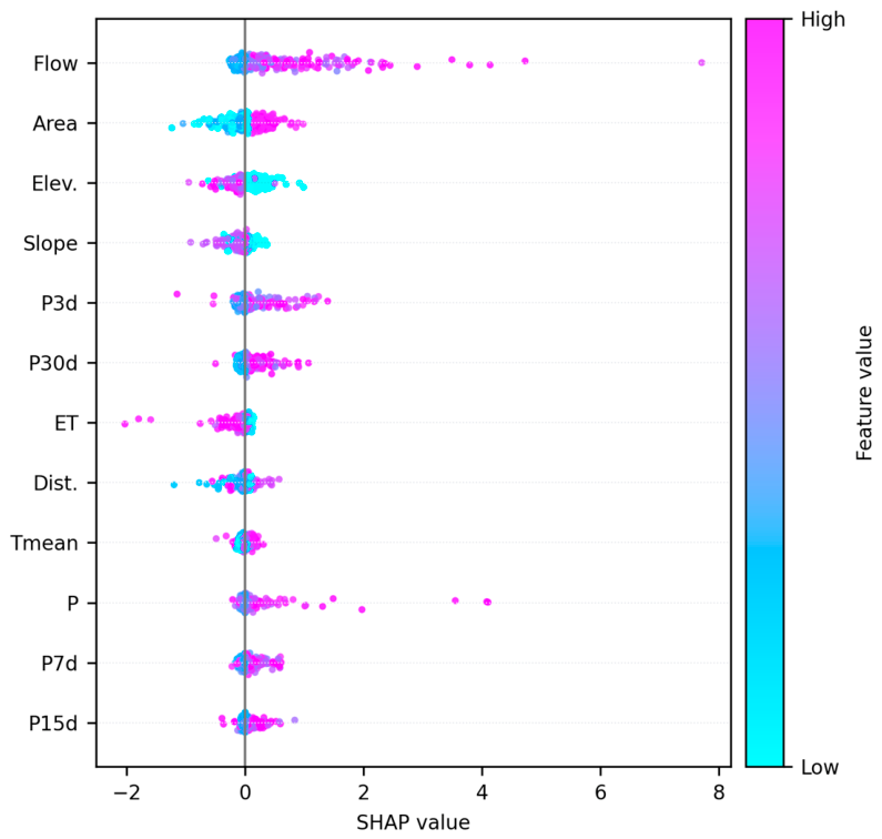
Figure 10 and Figure 11 show that donor-station discharge was the most important input information for HEG-LSTM, with a normalized SHAP importance of 0.251. The normalized importance values for drainage area, elevation, and slope were 0.154, 0.128, and 0.081, respectively, indicating that static basin attributes also played an important role in cross-section transferability. Antecedent precipitation accumulated over 3 d and 30 d had importance values of 0.065 and 0.063, respectively, showing that the model relies not only on the integrated hydrological state represented by donor-station discharge but also on local antecedent wetness conditions when identifying streamflow responses. The SHAP results can be interpreted as a three-layer information structure. Donor-station discharge represents dynamic hydrological connectivity and provides information on upstream wetness, runoff generation, and channel propagation. Static attributes, particularly drainage area and elevation, provide a spatial basis for distinguishing the scale and topographic setting of each section. Antecedent precipitation supplements these two information sources by representing local wetness conditions that may not be fully reflected in donor discharge. The prominence of donor flow is therefore consistent with the superior performance of S3, in which upstream and downstream information jointly contributes to the estimation of the intermediate section.

Figure 10. SHAP feature importance across scenarios.

Figure 11. SHAP summary plot for HEG-LSTM.

The importance of donor-station discharge varied substantially across scenarios. Under S3, its SHAP importance reached 0.337, exceeding the values of 0.237 under S1 and 0.200 under S2. This result indicates that when information from upstream and downstream stations is jointly used, the model relies more strongly on cross-section streamflow information. At the same time, drainage area and elevation were relatively more important under S2, suggesting that when downstream information alone is used to estimate an upstream section, the model may rely more on static attributes to distinguish differences in basin scale and topography among sections.

Evapotranspiration, mean air temperature, and same-day precipitation had relatively low importance, but this does not imply that these variables lack hydrological relevance. They may share substantial information with donor discharge and antecedent precipitation and therefore exhibit lower marginal contributions in SHAP attribution. In particular, mean air temperature contained a certain proportion of gap-filled values, and its importance should be interpreted cautiously. SHAP reflects the dependence of the trained model on different variables rather than strict causal contributions of those variables to streamflow variation.

Overall, the feature-attribution results indicate that cross-section estimation by HEG-LSTM depends on both dynamic hydrological connectivity and static spatial differences. Donor-station discharge provides integrated information on regional hydrological state and channel propagation, static attributes distinguish hydrological-response scales among sections, and antecedent precipitation supplements information on local wetness conditions. Grouped feature-removal experiments showed that mean NSE decreased from 0.7034 to 0.6115 after removing donor-station discharge, to 0.6768 after removing antecedent precipitation, and to 0.6767 after removing all meteorological inputs. Removing static attributes gave 0.7070. These results support the central role of donor discharge and antecedent wetness information, but also show that SHAP attribution represents conditional model dependence rather than an independent causal contribution. It is important to note that SHAP importance reflects the dependence of the trained model on the current data structure, rather than an independent causal effect of that estimation on streamflow. Donor discharge, antecedent precipitation, and static attributes may contain overlapping hydrological information. Therefore, a lower SHAP value for same-day precipitation, evapotranspiration, or air temperature should not be interpreted as evidence that these variables are hydrologically unimportant. Instead, the attribution results indicate that their marginal contribution was smaller after accounting for the information already represented by donor discharge and antecedent precipitation. This distinction is particularly relevant for nested basins, where strong dependence among hydrological variables may affect the apparent ranking of explanatory factors [43].

The interpretation results are also compared with recent interpretable machine-learning studies for ungauged-basin estimation. Xu, Y. et al. [44] used interpretable XGBoost with large-sample basin data to analyze cross-regional runoff estimation, whereas this study applies SHAP to an LSTM operating within a single nested station network and uses time-varying donor discharge as a key predictor. Thus, both studies use post-hoc interpretation to examine model reliance, but they address different transfer settings and model structures. In addition, interpretability studies of LSTM-based hydrological models caution that attribution values should not be treated as causal process evidence when predictors share hydrological information [41]. In our case, donor discharge, antecedent precipitation, and static attributes are correlated representations of catchment state and spatial setting. SHAP values are therefore interpreted as conditional model dependence, while the grouped feature-removal analysis is reported only as complementary sensitivity evidence for the incremental contribution of predictor groups.

5. Conclusions

This study developed an HEG-LSTM framework for streamflow estimation at ungauged sections in nested basins. The framework integrates local meteorological forcing, antecedent precipitation, static basin attributes, and scenario-permitted donor-station discharge to estimate daily streamflow at sections with missing or insufficient streamflow information. Three gauge-network scenarios were considered to analyze the effects of upstream and downstream station relationships on cross-section streamflow estimation. The following conclusions were obtained:

(1)

Compared with LSTM, overall hydrograph fitting and peak-magnitude estimation improved, but low-flow variation and peak timing did not improve consistently, indicating that the formation of low-flow processes remains difficult to represent using only the available meteorological variables, static attributes, and donor-station discharge.

(2)

The gauge-network scenarios showed different estimation capabilities and application boundaries. Use of the scenarios depends on donor direction and target position; S3 had the highest mean NSE in the tested intermediate combinations. These results indicate that streamflow-estimation capability in nested river networks is influenced not only by the number of donor stations but also by their relative positions to the target section, hydrological connectivity, and the effectiveness of the information they provide.

(3)

SHAP analysis showed that donor-station discharge was the most important model input, while drainage area, elevation, slope, and antecedent precipitation also made significant contributions to model transferability. This finding indicates that streamflow estimation at ungauged sections in nested river networks needs to consider dynamic hydrological connectivity, local wetness conditions, and spatial differences among contributing basins simultaneously.

The proposed framework provides a data-driven method for streamflow estimation and historical streamflow estimation at ungauged sections within nested river networks. Future research should incorporate channel travel time, tributary-confluence processes, reservoir operation, water-abstraction information, and broader station networks to improve the representation of low flow, peak occurrence time, and operational real-time applications.

References

- Kittel, C.M.M.; Arildsen, A.L.; Dybkjær, S.; Hansen, E.R.; Linde, I.; Slott, E.; Tøttrup, C.; Bauer-Gottwein, P. Informing hydrological models of poorly gauged river catchments–A parameter regionalization and calibration approach. J. Hydrol. 2020, 587, 124999. [Google Scholar] [CrossRef] [Scilit]
- Parajka, J.; Viglione, A.; Rogger, M.; Salinas, J.L.; Sivapalan, M.; Blöschl, G. Comparative assessment of predictions in ungauged basins–Part 1: Runoff-hydrograph studies. Hydrol. Earth Syst. Sci. 2013, 17, 1783–1795. [Google Scholar] [CrossRef] [Scilit]
- Sivapalan, M.; Takeuchi, K.; Franks, S.W.; Gupta, V.K.; Karambiri, H.; Lakshmi, V.; Liang, X.; McDonnell, J.J.; Mendiondo, E.M.; O’Connell, P.E.; et al. IAHS Decade on Predictions in Ungauged Basins (PUB), 2003–2012: Shaping an exciting future for the hydrological sciences. Hydrol. Sci. J. 2003, 48, 857–880. [Google Scholar] [CrossRef] [Scilit]
- Hrachowitz, M.; Savenije, H.H.G.; Blöschl, G.; McDonnell, J.J.; Sivapalan, M.; Pomeroy, J.W.; Arheimer, B.; Blume, T.; Clark, M.P.; Ehret, U.; et al. A decade of Predictions in Ungauged Basins (PUB)—A review. Hydrol. Sci. J. 2013, 58, 1198–1255. [Google Scholar] [CrossRef] [Scilit]
- Hu, C.; Xia, J.; She, D.; Jing, Z.; Hong, S.; Song, Z.; Wang, G. Parameter Regionalization With Donor Catchment Clustering Improves Urban Flood Modeling in Ungauged Urban Catchments. Water Resour. Res. 2024, 60, e2023WR035071. [Google Scholar] [CrossRef] [Scilit]
- Guo, Y.; Zhang, Y.; Zhang, L.; Wang, Z. Regionalization of Hydrological Modeling for Predicting Streamflow in Ungauged Catchments: A Comprehensive Review. WIREs Water 2021, 8, e1487. [Google Scholar] [CrossRef] [Scilit]
- Arsenault, R.; Brissette, F.P. Continuous streamflow prediction in ungauged basins: The effects of equifinality and parameter set selection on uncertainty in regionalization approaches. Water Resour. Res. 2014, 50, 6135–6153. [Google Scholar] [CrossRef] [Scilit]
- Merz, R.; Blöschl, G. Regionalisation of catchment model parameters. J. Hydrol. 2004, 287, 95–123. [Google Scholar] [CrossRef] [Scilit]
- Oudin, L.; Andréassian, V.; Perrin, C.; Michel, C.; Le Moine, N. Spatial proximity, physical similarity, regression and ungaged catchments: A comparison of regionalization approaches based on 913 French catchments. Water Resour. Res. 2008, 44, 2007wr006240. [Google Scholar] [CrossRef] [Scilit]
- Song, Z.; Xia, J.; Wang, G.; She, D.; Hu, C.; Hong, S. Regionalization of Hydrological Model Parameters Using Gradient Boosting Machine. Hydrol. Earth Syst. Sci. 2022, 26, 505–524. [Google Scholar] [CrossRef] [Scilit]
- Kratzert, F.; Klotz, D.; Brenner, C.; Schulz, K.; Herrnegger, M. Rainfall–runoff modelling using Long Short-Term Memory (LSTM) networks. Hydrol. Earth Syst. Sci. 2018, 22, 6005–6022. [Google Scholar] [CrossRef] [Scilit]
- Kratzert, F.; Klotz, D.; Shalev, G.; Klambauer, G.; Hochreiter, S.; Nearing, G. Towards learning universal, regional, and local hydrological behaviors via machine learning applied to large-sample datasets. Hydrol. Earth Syst. Sci. 2019, 23, 5089–5110. [Google Scholar] [CrossRef] [Scilit]
- Arsenault, R.; Martel, J.-L.; Brunet, F.; Brissette, F.; Mai, J. Continuous streamflow prediction in ungauged basins: Long short-term memory neural networks clearly outperform traditional hydrological models. Hydrol. Earth Syst. Sci. 2023, 27, 139–157. [Google Scholar] [CrossRef] [Scilit]
- Kratzert, F.; Gauch, M.; Klotz, D.; Nearing, G. HESS Opinions: Never train a Long Short-Term Memory (LSTM) network on a single basin. Hydrol. Earth Syst. Sci. 2024, 28, 4187–4201. [Google Scholar] [CrossRef] [Scilit]
- Kratzert, F.; Klotz, D.; Herrnegger, M.; Sampson, A.K.; Hochreiter, S.; Nearing, G.S. Toward Improved Predictions in Ungauged Basins: Exploiting the Power of Machine Learning. Water Resour. Res. 2019, 55, 11344–11354. [Google Scholar] [CrossRef] [Scilit]
- Li, X.; Khandelwal, A.; Jia, X.; Cutler, K.; Ghosh, R.; Renganathan, A.; Xu, S.; Tayal, K.; Nieber, J.; Duffy, C.; et al. Regionalization in a Global Hydrologic Deep Learning Model: From Physical Descriptors to Random Vectors. Water Resour. Res. 2022, 58, e2021WR031794. [Google Scholar] [CrossRef] [Scilit]
- Feng, D.; Fang, K.; Shen, C. Enhancing Streamflow Forecast and Extracting Insights Using Long Short-Term Memory Networks With Data Integration at Continental Scales. Water Resour. Res. 2020, 56, e2019WR026793. [Google Scholar] [CrossRef] [Scilit]
- Vischer, M.A.; Otero, N.; Ma, J. Spatially Resolved Rainfall Streamflow Modeling in Central Europe. Hydrol. Earth Syst. Sci. 2025, 29, 5233–5250. [Google Scholar] [CrossRef] [Scilit]
- Yu, Q.; Tolson, B.A.; Shen, H.; Han, M.; Mai, J.; Lin, J. Enhancing long short-term memory (LSTM)-based streamflow prediction with a spatially distributed approach. Hydrol. Earth Syst. Sci. 2024, 28, 2107–2122. [Google Scholar] [CrossRef] [Scilit]
- Mosaffa, H.; Pappenberger, F.; Prudhomme, C.; Chantry, M.; Rüdiger, C.; Cloke, H. A GNN routing module is all you need for LSTM Rainfall–Runoff models. Hydrol. Earth Syst. Sci. 2026, 30, 2079–2092. [Google Scholar] [CrossRef] [Scilit]
- Vaheddoost, B.; Yilmaz, M.U.; Safari, M.J.S. Estimation of flow duration and mass flow curves in ungauged tributary streams. J. Clean. Prod. 2023, 409, 137246. [Google Scholar] [CrossRef] [Scilit]
- Liu, J.; Koch, J.; Stisen, S.; Troldborg, L.; Schneider, R.J.M. A national-scale hybrid model for enhanced streamflow estimation–consolidating a physically based hydrological model with long short-term memory (LSTM) networks. Hydrol. Earth Syst. Sci. 2024, 28, 2871–2893. [Google Scholar] [CrossRef] [Scilit]
- Martel, J.-L.; Arsenault, R.; Turcotte, R.; Castañeda-Gonzalez, M.; Brissette, F.; Armstrong, W.; Mailhot, E.; Pelletier-Dumont, J.; Lachance-Cloutier, S.; Rondeau-Genesse, G.; et al. Exploring the ability of LSTM-based hydrological models to simulate streamflow time series for flood frequency analysis. Hydrol. Earth Syst. Sci. 2025, 29, 4951–4968. [Google Scholar] [CrossRef] [Scilit]
- Ma, K.; Feng, D.; Lawson, K.; Tsai, W.P.; Liang, C.; Huang, X.; Sharma, A.; Shen, C. Transferring Hydrologic Data Across Continents—Leveraging Data-Rich Regions to Improve Hydrologic Prediction in Data-Sparse Regions. Water Resour. Res. 2021, 57, e2020WR028600. [Google Scholar] [CrossRef] [Scilit]
- Fang, K.; Kifer, D.; Lawson, K.; Feng, D.; Shen, C. The Data Synergy Effects of Time-Series Deep Learning Models in Hydrology. Water Resour. Res. 2022, 58, e2021WR029583. [Google Scholar] [CrossRef] [Scilit]
- Yang, Y.; Pan, M.; Feng, D.; Xiao, M.; Dixon, T.; Hartman, R.; Shen, C.; Song, Y.; Sengupta, A.; Delle Monache, L.; et al. Improving Streamflow Simulation through Machine Learning-Powered Data Integration and Its Potential for Forecasting in the Western U.S. Hydrol. Earth Syst. Sci. 2025, 29, 5453–5476. [Google Scholar] [CrossRef] [Scilit]
- Hochreiter, S.; Schmidhuber, J. Long Short-Term Memory. Neural Comput. 1997, 9, 1735–1780. [Google Scholar] [CrossRef] [Scilit] [PubMed]
- Nash, J.E.; Sutcliffe, J.V. River Flow Forecasting through Conceptual Models Part I—A Discussion of Principles. J. Hydrol. 1970, 10, 282–290. [Google Scholar] [CrossRef] [Scilit]
- Lundberg, S.M.; Lee, S.I. A Unified Approach to Interpreting Model Predictions. In Proceedings of the 31st International Conference on Neural Information Processing Systems, Long Beach, CA, USA, 4–9 December 2017; pp. 4766–4777. [Google Scholar]
- Frame, J.M.; Kratzert, F.; Klotz, D.; Gauch, M.; Shalev, G.; Gilon, O.; Qualls, L.M.; Gupta, H.V.; Nearing, G.S. Deep Learning Rainfall–Runoff Predictions of Extreme Events. Hydrol. Earth Syst. Sci. 2022, 26, 3377–3392. [Google Scholar] [CrossRef] [Scilit]
- Klotz, D.; Kratzert, F.; Gauch, M.; Keefe Sampson, A.; Brandstetter, J.; Klambauer, G.; Hochreiter, S.; Nearing, G. Uncertainty Estimation with Deep Learning for Rainfall–Runoff Modeling. Hydrol. Earth Syst. Sci. 2022, 26, 1673–1693. [Google Scholar] [CrossRef] [Scilit]
- Knoben, W.J.M.; Freer, J.E.; Woods, R. Technical Note: Inherent Benchmark or Not? Comparing Nash–Sutcliffe and Kling–Gupta Efficiency Scores. Hydrol. Earth Syst. Sci. 2019, 23, 4323–4331. [Google Scholar] [CrossRef] [Scilit]
- Gupta, H.V.; Kling, H.; Yilmaz, K.K.; Martinez, G.F. Decomposition of the Mean Squared Error and NSE Performance Criteria: Implications for Improving Hydrological Modelling. J. Hydrol. 2009, 377, 80–91. [Google Scholar] [CrossRef] [Scilit]
- Cho, K.; Kim, Y. Improving streamflow prediction in the WRF-Hydro model with LSTM networks. J. Hydrol. 2022, 605, 127297. [Google Scholar] [CrossRef] [Scilit]
- Sun, A.Y.; Jiang, P.; Yang, Z.L.; Xie, Y.; Chen, X. A Graph Neural Network (GNN) Approach to Basin-Scale River Network Learning: The Role of Physics-Based Connectivity and Data Fusion. Hydrol. Earth Syst. Sci. 2022, 26, 5163–5184. [Google Scholar] [CrossRef] [Scilit]
- Gauch, M.; Mai, J.; Lin, J. The Proper Care and Feeding of CAMELS: How Limited Training Data Affects Streamflow Prediction. Environ. Model. Softw. 2021, 135, 104926. [Google Scholar] [CrossRef] [Scilit]
- Wi, S.; Steinschneider, S. On the Need for Physical Constraints in Deep Learning Rainfall–Runoff Projections under Climate Change: A Sensitivity Analysis to Warming and Shifts in Potential Evapotranspiration. Hydrol. Earth Syst. Sci. 2024, 28, 479–503. [Google Scholar] [CrossRef] [Scilit]
- Gauch, M.; Kratzert, F.; Klotz, D.; Nearing, G.; Lin, J.; Hochreiter, S. Rainfall–Runoff Prediction at Multiple Timescales with a Single Long Short-Term Memory Network. Hydrol. Earth Syst. Sci. 2021, 25, 2045–2062. [Google Scholar] [CrossRef] [Scilit]
- Baste, S.; Klotz, D.; Acuña Espinoza, E.; Bárdossy, A.; Loritz, R. Unveiling the Limits of Deep Learning Models in Hydrological Extrapolation Tasks. Hydrol. Earth Syst. Sci. 2025, 29, 5871–5891. [Google Scholar] [CrossRef] [Scilit]
- Xiang, X.; Guo, S.; Li, C.; Wang, Y. An Explainable Deep Learning Model Based on Hydrological Principles for Flood Simulation and Forecasting. Hydrol. Earth Syst. Sci. 2025, 29, 7217–7239. [Google Scholar] [CrossRef] [Scilit]
- De la Fuente, L.A.; Ehsani, M.R.; Gupta, H.V.; Condon, L.E. Toward Interpretable LSTM-Based Modeling of Hydrological Systems. Hydrol. Earth Syst. Sci. 2024, 28, 945–971. [Google Scholar] [CrossRef] [Scilit]
- Ouyang, W.; Lawson, K.; Feng, D.; Ye, L.; Zhang, C.; Shen, C. Continental-Scale Streamflow Modeling of Basins with Reservoirs: Towards a Coherent Deep-Learning-Based Strategy. J. Hydrol. 2021, 599, 126455. [Google Scholar] [CrossRef] [Scilit]
- Lees, T.; Reece, S.; Kratzert, F.; Klotz, D.; Gauch, M.; De Bruijn, J.; Kumar Sahu, R.; Greve, P.; Slater, L.; Dadson, S.J. Hydrological Concept Formation Inside Long Short-Term Memory (LSTM) Networks. Hydrol. Earth Syst. Sci. 2022, 26, 3079–3101. [Google Scholar] [CrossRef] [Scilit]
- Xu, Y.; Lin, K.; Hu, C.; Wang, S.; Wu, Q.; Zhang, J.; Xiao, M.; Luo, Y. Interpretable machine learning on large samples for supporting runoff estimation in ungauged basins. J. Hydrol. 2024, 639, 131598. [Google Scholar] [CrossRef] [Scilit]
Disclaimer/Publisher’s Note: The statements, opinions and data contained in all publications are solely those of the individual author(s) and contributor(s) and not of MDPI and/or the editor(s). MDPI and/or the editor(s) disclaim responsibility for any injury to people or property resulting from any ideas, methods, instructions or products referred to in the content. |
© 2026 by the authors. Licensee MDPI, Basel, Switzerland. This article is an open access article distributed under the terms and conditions of the Creative Commons Attribution (CC BY) license.