Data-Driven BOD₅ Prediction in Urban Drainage Networks Using a BP Neural Network Under Limited Monitoring Conditions

Abstract

To address the engineering challenges of long detection cycles and the inability to provide real-time early warning for the traditional measurement of 5-day biochemical oxygen demand (BOD₅) in drainage networks, coupled with the limited availability of monitored indicators in practice, this study proposes a BOD₅ concentration prediction method based on a BP neural network. Based on 10,511 sets of field measurements from a city’s drainage network, only three routinely measurable indicators, chemical oxygen demand (COD), ammonia nitrogen (NH₄⁺-N), and total phosphorus (TP), were selected as input features. A COD-only baseline model was first constructed to validate the reliability of the core predictive factor (R² = 0.9401). NH₄⁺-N and TP were then incorporated to build a three-feature synergistic prediction model, which improved the R² to 0.9541. By comparing three optimization algorithms (L-BFGS, Adam, and SGD) and performing hyperparameter optimization, the final test-set R² reached 0.957 with an MAE of 8.834 mg/L (MAPE = 12.89%), representing a practical error of approximately 10.3% of the mean BOD₅ concentration. The prediction accuracy was significantly superior to support vector regression (SVR, R² = 0.930) and multiple linear regression (MLR, R² = 0.955). Generalization ability was validated using three external independent datasets from Jinan (China), Hohhot (China), and Melbourne (Australia). The results show that the model maintains reasonable predictive capability within the same region (R²= 0.844), but accuracy declines substantially when transferring across regions (MAPE increasing from 12.89% to 35.07–58.63%) and countries. This method provides a high-accuracy, low-cost, real-time estimation scheme for early warning of water quality in drainage networks under limited monitoring conditions.

1. Introduction

Urban drainage networks serve the core function of collecting and conveying domestic sewage, industrial wastewater, and stormwater, and their operational status is directly linked to urban water environment safety and public health. With rapid urbanization in China, the total length of urban drainage pipelines reached approximately 1 million km by 2025 [1]. However, a large proportion of existing infrastructure consists of aging pipes prone to sedimentation, blockages, and corrosion [2,3]. Biochemical oxygen demand (BOD) is a core indicator of organic pollution, reflecting both the environmental hazard potential of sewage and the microbial activity, organic matter deposition, and anaerobic decomposition within pipes [4]. Specifically, BOD₅ concentration is closely linked to pipe sedimentation, corrosion risk, and the generation of toxic gases such as hydrogen sulfide (H₂S) [5,6]. Mechanistically, organic matter deposited in sewer sediments undergoes microbial degradation, elevating BOD₅; under anaerobic conditions, sulfate-reducing bacteria convert sulfate to H₂S, which volatilizes and is oxidized to sulfuric acid on moist pipe surfaces, progressively degrading the concrete matrix [2,3,5,6]. Therefore, rapid and accurate BOD5 monitoring is of significant engineering value for pipeline water quality assessment and maintenance guidance. However, the standard BOD₅ method requires a five-day incubation, yielding results only after 5 days [7], which precludes real-time decision support for drainage network operations and early pollution warning.

Existing water quality prediction methods fall into three categories: mechanistic, statistical, and machine learning models. Mechanistic models (e.g., QUAL2E, SWMM water quality modules) [8] offer clear physical interpretation but require extensive parameter calibration, limiting their applicability in highly disturbed environments such as drainage networks [9]. Statistical models (e.g., MLR, ARIMA) [10] are computationally simple but struggle to capture non-linear relationships in water quality data. In recent years, machine learning methods, particularly artificial neural networks (ANNs), have become prominent due to their non-linear mapping and self-learning capabilities. The BP neural network, with its simple structure and mature training algorithms, has been widely applied [11,12,13], including water quality prediction in Lake Taihu [14] and Malaysian rivers [15], with further applications in water quality estimation [16,17,18]. For BOD₅ prediction specifically, support vector regression has been used for real-time effluent prediction [19,20], and various machine learning algorithms have been applied in wastewater treatment plants [21]. However, most studies relied on idealized data-complete scenarios or high-frequency continuous monitoring with temporal characteristics to build sequential models such as LSTM [22].

The current challenge lies in the constraints of practical drainage network monitoring. Most monitoring stations are equipped with only a few online devices for core indicators (COD, NH₄⁺-N, TP), severely limiting feature dimensionality. Additionally, water quality sampling is conducted as independent observations at irregular intervals, yielding data without continuous time-series characteristics and making time-series models difficult to apply [23]. Furthermore, a critical distinction between sewer network wastewater and WWTP influent/effluent that has been insufficiently addressed is that sewer wastewater exhibits greater compositional variability due to intermittent industrial discharges, sediment resuspension during wet-weather events, in-pipe biological transformations, and the absence of steady-state conditions, making BOD₅ prediction fundamentally more challenging. How to achieve accurate BOD₅ prediction under these constraints of “low-dimensional features and non-temporal data” represents an overlooked gap in current research.

To address the above limitations, this study proposes a BOD₅ prediction method using a BP neural network with limited input features. Based on 10,511 sets of field measurements from an actual drainage network, the study selects only COD, NH₄⁺-N, and TP as input features without relying on temporal information. A progressive validation strategy is adopted: (1) a COD-only baseline model validates the core predictive factor; (2) multi-feature synergistic prediction is assessed by introducing NH₄⁺-N and TP; (3) three optimization algorithms (L-BFGS, Adam, and SGD) are compared with grid-search hyperparameter optimization, alongside SVR and MLR benchmarks; and (4) three external datasets from Jinan and Hohhot (China) and Melbourne (Australia) are used to evaluate cross-regional generalization ability, aiming to provide a high-accuracy, engineering-practical scheme for water quality early warning under limited monitoring conditions.

2. Data and Methodology

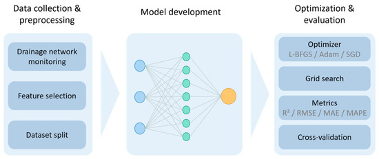
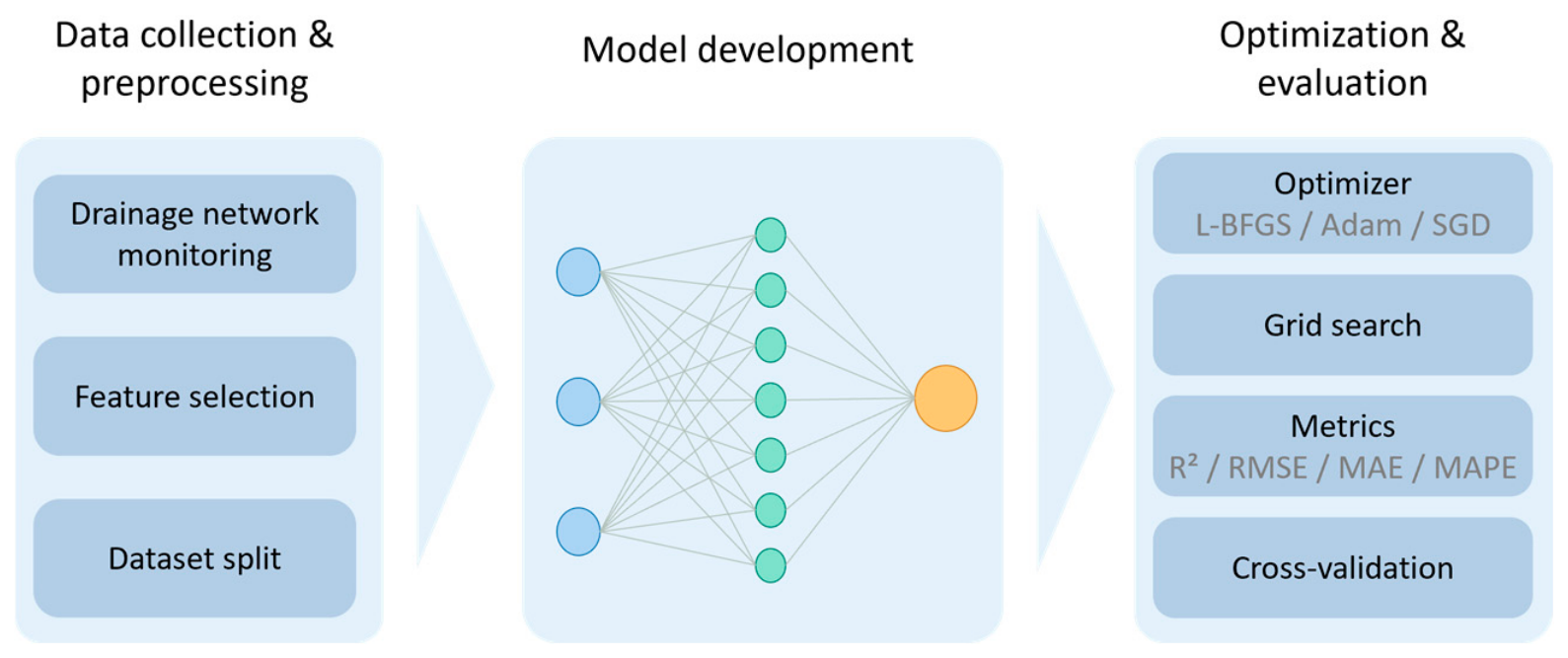
The overall methodology framework consists of three integrated components: (1) data collection and preprocessing (Section 2.1), encompassing water quality sampling, sample preservation protocols, and input feature selection; (2) model development (Section 2.2), including BP neural network architecture, mathematical formulation, and training configuration; and (3) optimization and evaluation strategy (Section 2.3), covering algorithm comparison, hyperparameter tuning, baseline benchmarking, and multi-metric assessment, as shown in Figure 1.

Figure 1. Schematic diagram of the methodology.

2.1. Data Collection and Preprocessing

The data used in this study originate from water quality sampling records at monitoring cross-sections of the main trunk pipelines of a city’s drainage network, spanning January 2022 to December 2024, yielding a total of 10,511 valid samples (outliers removed per the 3 sigma criterion). Each sample comprises four indicators: COD, NH₄⁺-N, TP, and BOD₅. All samples originate from independent sampling at different monitoring locations with non-fixed time intervals and no continuous time-series characteristics; therefore, all samples are treated as independent and identically distributed (i.i.d.) static data. To ensure data reliability, all samples were analyzed within 6 h of collection, stored in clean amber glass bottles at 4 °C in dark conditions during transport, and preserved according to standard methods [7].

COD, NH₄⁺-N, and TP were selected as input features based on three considerations: (1) theoretical relevance—COD and BOD₅ both characterize organic matter content with strong correlation, while NH₄⁺-N and TP reflect nutrient levels associated with organic degradation; (2) data accessibility—the monitoring stations are equipped with online sensors for only these four indicators; and (3) engineering value—prediction methods based on limited core indicators are practical for regions with constrained monitoring conditions.

To evaluate data quality and the effect of outlier removal, the 3σ criterion was applied. Table 1 presents the statistical comparison before and after outlier elimination. After removal, the coefficient of variation for each indicator ranges from 65% to 72%, indicating a wide concentration spectrum. All four indicators exhibit a right-skewed distribution, with the bulk of the data concentrated in the low-to-medium concentration ranges. The final dataset comprises 10,511 valid samples (originally 10,893), with the maximum values of COD, NH₄⁺-N, TP, and BOD₅ reduced from 693, 133, 26.4, and 438 mg/L to 589, 120, 11.4, and 278 mg/L, respectively, effectively eliminating extreme outliers while preserving the overall distribution shape.

Table 1. Descriptive Statistics of Water Quality Indicators.

Indicator	Original					Final
	Mean	Std. Dev.	Coeff. of Variation (%)	Min.	Max	Mean	Std. Dev.	Coeff. of Variation (%)	Min.	Max
COD (mg/L)	196.62	130.97	66.61	4	693	191.91	124.98	65.13	4	589
NH4+-N (mg/L)	39.91	26.81	67.18	0.02	133	39.44	26.37	66.85	0.02	120
TP (mg/L)	3.84	2.59	67.31	0.01	26.4	3.77	2.49	66.09	0.01	11.4
BOD5 (mg/L)	88.53	66.41	75.01	0.39	438	85.71	61.69	71.97	0.39	278

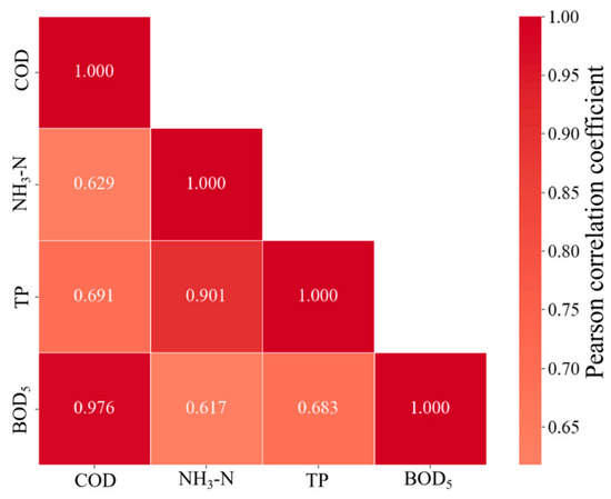
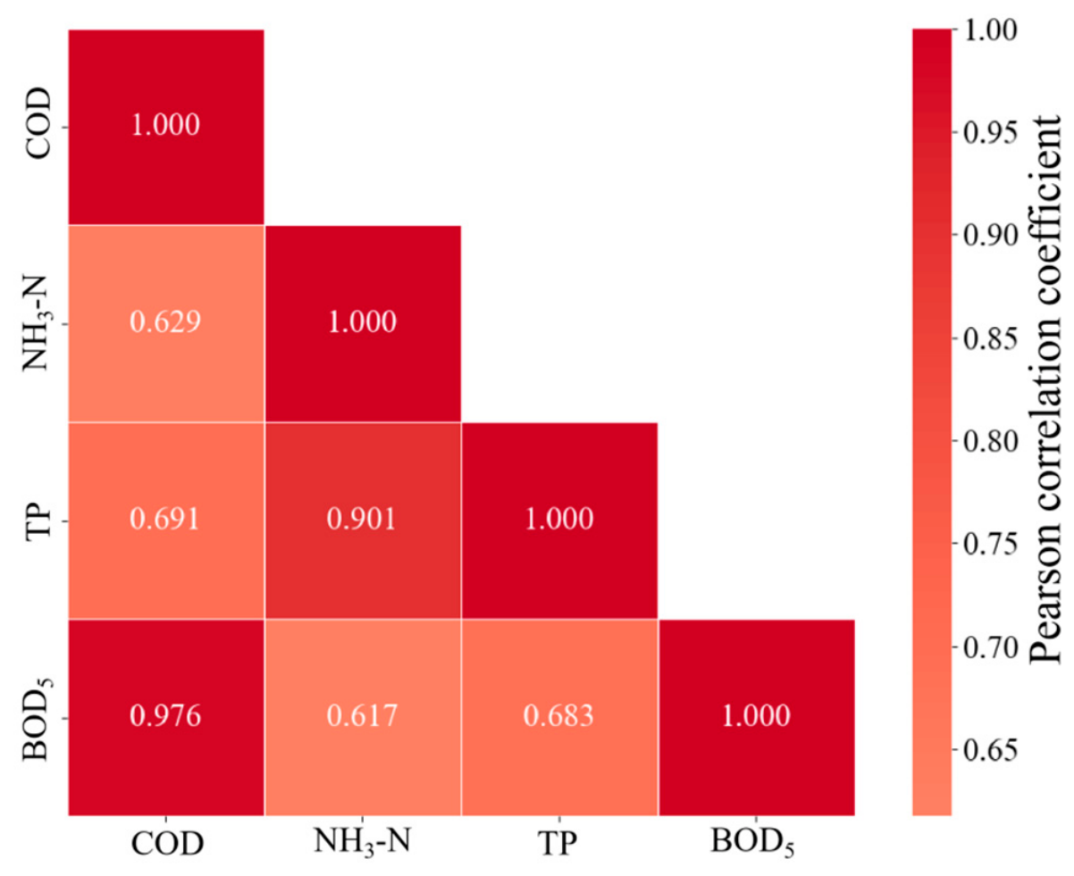
The coefficient of variation for each indicator ranges from 51% to 72%, covering a wide concentration range from low to high pollution. All four indicators exhibited right-skewed distributions with extreme values at the high-concentration end, providing a rich data foundation for model training. Pearson correlation analysis (Figure 2) revealed that BOD5 exhibited an extremely strong positive correlation with COD (r = 0.976), moderate-to-strong correlations with NH₄⁺-N (r = 0.745) and TP (r = 0.758), and a strong intercorrelation between NH₄⁺-N and TP (r = 0.901). These results confirm that COD possesses strong standalone predictive potential, while the multi-feature synergistic approach is supported by the covariation of pollutant concentrations.

Figure 2. Correlation heatmap of each indicator with BOD₅.

2.2. Model Development

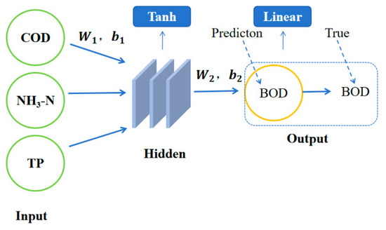
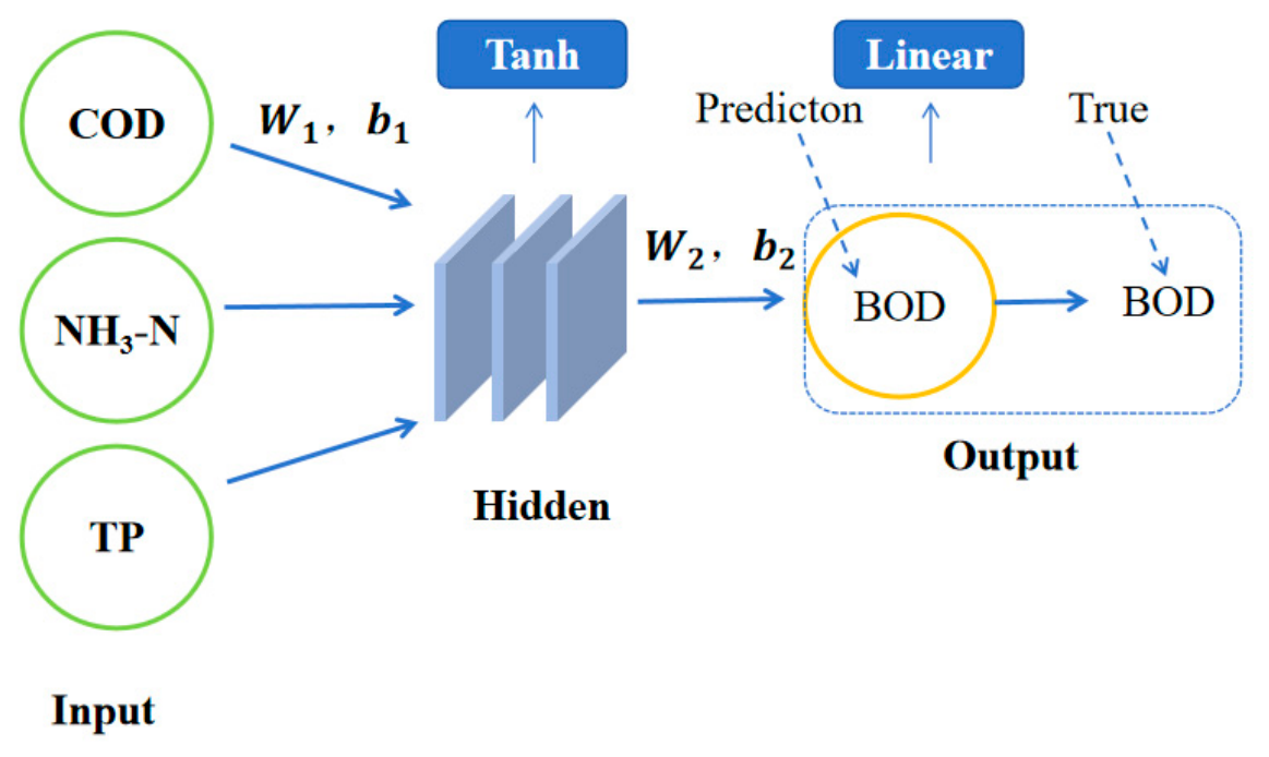
This study employed a single-hidden-layer BP neural network to construct the BOD₅ prediction model (Figure 3). The BP neural network is a multi-layer feedforward network based on the error back-propagation algorithm, comprising an input layer, a hidden layer, and an output layer. The learning process consists of forward propagation, where signals are transmitted from the input layer through the hidden layer to the output layer, and backward propagation, where the error between predicted and observed values is propagated backward to update connection weights via the chain rule. This mechanism enables the network to approximate non-linear mapping relationships [24], making it suitable for the multi-factor coupling scenario in this study.

Figure 3. Network structure of the BOD₅ prediction model.

The mathematical formulation of the BP neural network is described as follows:

Forward propagation—hidden layer output:

$$h=f\left(W_1·x+b_1\right)=tanh\left(W_1·x+b_1\right)$$

Forward propagation—output layer:

$$\mathrm{ŷ}=W_2·h+b_2$$

Loss function (Mean Squared Error):

L = (1/n) · Σ_i=1ⁿ (y_i − ŷ_i)²

$$L={\displaystyle \frac{1}{n}}·{\displaystyle \sum _{i=1}^n}{\left(y_i-{\mathrm{ŷ}}_i\right)}^2$$

Weight update (backpropagation with learning rate η):

$$W_{t+1}=W_t-\eta ·{\displaystyle \frac{\partial L}{\partial W}}$$

where x is the input vector (COD, NH₄⁺-N, and TP); W₁ and W₂ are the weight matrices for the hidden and output layers, respectively; b₁ and b₂ are bias vectors; f(·) is the activation function (tanh); h is the hidden layer output; ŷ is the predicted BOD₅ concentration; y_i is the observed BOD₅ value; n is the number of samples; L is the loss function; η is the learning rate; and ${\displaystyle \frac{\partial L}{\partial W}}$ is the gradient of the loss with respect to the weights.

The number of hidden-layer nodes was determined using the empirical formula:

$$m=\sqrt{n+l}+a$$

where n is the number of input-layer nodes, l is the number of output-layer nodes, and a is a tuning constant between 1 and 10.

For the COD-only model (n = 1, l = 1), the optimal number of nodes was determined to be 5 through experimental comparison; for the three-feature model (n = 3, l = 1), the optimal number was 7.

The baseline model was first constructed with COD as the sole input and a single input-layer node. The number of hidden-layer nodes was determined to be 5 through empirical formulas and experimental comparison. This baseline model aimed to establish a performance benchmark and validate the reliability of COD as the core predictive indicator. Subsequently, the input features were extended to three: COD, NH₄⁺-N, and TP, increasing the input-layer nodes to 3, and the hidden-layer nodes were optimized to 7, forming a three-feature model to quantify the improvement in prediction accuracy achieved by synergistic multi-feature prediction.

The hyperbolic tangent (tanh) function was adopted as the activation function for the hidden layer across all models because its zero-centering property facilitates network convergence. A linear activation function was used in the output layer to produce continuous predictions of BOD₅ concentration. The dataset was randomly partitioned into training, validation, and test sets in a 7:1.5:1.5 ratio (7357, 1577, and 1577 samples, respectively). To eliminate dimensional effects, all variables were normalized to the [0, 1] interval using min-max scaling.

2.3. Optimization and Evaluation Strategy

The choice of optimization algorithm has a decisive impact on the convergence speed and prediction accuracy of the BP neural network. This study selected three representative algorithms for systematic comparison: L-BFGS (Limited-memory BFGS) quasi-Newton method, which offers fast convergence and insensitivity to learning rate, making it particularly suitable for small- to medium-sized datasets [25]; Adam (Adaptive Moment Estimation), an adaptive learning-rate algorithm that combines the advantages of momentum methods and RMSProp, and is one of the most widely applied optimizers today [26]; and stochastic gradient descent with momentum (SGD with Momentum), which effectively suppresses oscillations and accelerates convergence in mini-batch training [27].

For hyperparameter optimization, a combination of grid search and five-fold cross-validation was employed. Parameters optimized included: the number of hidden-layer nodes (single-layer structures: 3, 5, 7, 9, 11; two-layer structures: (3,3), (5,5), (7,7)); regularization coefficient α (0.0001, 0.001, 0.01); activation function (Tanh, ReLU); and initial learning rate (for Adam: 0.001–0.01). The average RMSE was used as the evaluation metric to determine the optimal parameter combination. All models employed an early stopping strategy: training was terminated when the validation loss did not decrease for 10 consecutive epochs to prevent overfitting.

To comprehensively evaluate the performance of the BP neural network, support vector regression (SVR) and multiple linear regression (MLR) were selected as baseline models for comparison. SVR adopted a radial basis function (RBF) kernel, with the penalty parameter C and kernel parameter γ optimized via grid search. MLR used COD, NH₄⁺-N, and TP as independent variables and BOD₅ as the dependent variable, with regression coefficients estimated by the least-squares method.

For model evaluation, four metrics were adopted: root mean square error (RMSE), mean absolute error (MAE), coefficient of determination (R²), and mean absolute percentage error (MAPE), providing a multidimensional assessment of prediction performance in terms of error magnitude, goodness of fit, and relative deviation.

3. Results and Discussion

3.1. Feature Contribution and Model Performance Comparison

To systematically evaluate the effects of different feature combinations and optimization algorithms on BOD₅ prediction accuracy, this study constructed and compared multiple models, as shown in Table 2.

Table 2. Model performance comparison for different input feature groups.

Input	R2	Improvement (%)
COD	0.9401	—
COD + TP	0.9370	−0.3
COD + NH4+-N	0.9452	+0.5
COD + NH4+-N + TP	0.9541	+1.5

First, the baseline model with COD as the sole input achieved an R² of 0.9401, RMSE of 15.046 mg/L, and MAE of 10.827 mg/L on the test set. This result confirms the extremely strong correlation between COD and BOD₅ (r = 0.976), indicating that even when COD is monitored alone, the BP neural network can achieve a reasonably reliable estimate of BOD₅, providing the most parsimonious prediction scheme for scenarios with limited monitoring indicators.

Building on this, NH₄⁺-N and TP were progressively introduced to examine the effects of synergistic prediction across multiple features. As shown in Table 2, introducing NH₄⁺-N alone increased R² to 0.9452, whereas introducing TP alone slightly decreased R² to 0.9370, suggesting that a single TP feature may introduce noise. TP concentrations in drainage networks are influenced by multiple sources, including detergents, industrial phosphorus discharges, and sediment release from pipe deposits, and their association with BOD₅ is less direct than that of COD. When fluctuations in TP data unrelated to organic matter degradation dominate, they can introduce noise signals that interfere with the stable mapping relationship between COD and BOD₅. However, when TP is used alongside NH₄⁺-N, the two together characterize the overall level of microbial metabolism, suppressing noise and strengthening the signal.

When all three features, COD, NH₄⁺-N, and TP, were used together, the model R² reached 0.9541, an improvement of 1.5% over the baseline model. This result indicates that NH₄⁺-N and TP provide supplementary information on organic matter degradation processes from the perspectives of nitrogen and phosphorus, forming a synergistic complementarity with COD that effectively compensates for BOD₅ variations not fully captured by COD alone.

After hyperparameter optimization using grid search with 5-fold cross-validation, the optimal configuration for the BP-LBFGS model was a single hidden layer with 3 nodes, a regularization coefficient of 0.0001, and the Tanh activation function.

To provide a transparent view of hyperparameter selection, Table 3 lists representative combinations from the grid search. The optimal configuration was a single hidden layer with 3 nodes, α = 0.0001, and Tanh activation (RMSE = 12.753, R² = 0.9573). Increasing network depth to (7,7) yielded no significant improvement (RMSE = 12.765), while two-layer structures with ReLU caused training divergence (R² ≈ 0). Grid-search results achieved an R² of 0.957, an RMSE of 12.753 mg/L, an MAE of 8.834 mg/L, and a MAPE of 12.887% on the test set.

Table 3. Representative hyperparameter combinations from grid search.

Hidden Layers	Regularization (α)	Activation	RMSE (mg/L)	R2
(3,)	0.0001	Tanh	12.753	0.9573
(3,)	0.0001	ReLU	13.039	0.9554
(3,)	0.01	Tanh	12.757	0.9572
(7,7)	0.0001	Tanh	12.765	0.9572
(5,5)	0.01	ReLU	12.931	0.9561
(3,3)	0.0001	ReLU	61.752	−0.0003

To verify the superiority of the BP neural network under limited-indicator conditions, the optimized BP-LBFGS model was compared with BP-SGD, SVR, and MLR, as shown in Table 4.

Table 4. Prediction performance comparison of all models.

Model	RMSE (mg/L)	MAE (mg/L)	R2	MAPE (%)
COD-only	15.046	10.827	0.940	39.18
BP-LBFGS	12.753	8.834	0.957	12.89
BP-Adam	12.931	9.158	0.956	16.14
BP-SGD	14.059	10.312	0.949	40.57
SVR	16.439	13.695	0.930	123.59
MLR	13.141	9.502	0.955	32.20

The results show that BP-LBFGS performed best across all evaluation metrics: its R² (0.957) was approximately 0.8% higher than BP-SGD, 2.9% higher than SVR, and 0.2% higher than MLR. Its MAE (8.834 mg/L) was the lowest among all models. SVR, unable to effectively capture the complex non-linear interactions among multiple features, performed the poorest (R² = 0.930). MLR performed reasonably overall, but the fitting in regions with large data fluctuations was clearly inferior to that of the BP network. The above comparisons confirm the fitting advantage of BP neural networks for low-dimensional, non-linear water quality data. The MAE of 8.834 mg/L represents approximately 10.3% of the mean BOD₅ concentration (85.71 mg/L) and only 3.2% of the full measurement range (0–278 mg/L), indicating high practical reliability. Compared with SVR, the BP-LBFGS model reduced MAE by 35.5% (from 13.695 to 8.834 mg/L) and RMSE by 22.4% (from 16.439 to 12.753 mg/L). Compared with MLR, MAE was reduced by 7.0% and RMSE by 2.9%. These reductions demonstrate that, while the R² improvement over MLR is modest (0.2%), the practical error reduction is more substantial, particularly in reducing large deviations.

3.2. Generalization Ability Validation with Multi-Source Data

To examine the model’s applicability across regions with varying water quality characteristics, the optimized three-feature BP-LBFGS model was applied to three external independent datasets from Jinan (China), Hohhot (China), and Melbourne (Australia). The results are presented in Table 5.

Table 5. Generalization performance of the model on external datasets.

Dataset	Sample Size	Input Features	R2	RMSE (mg/L)	MAPE (%)
Original test set	1577	COD + NH4+-N + TP	0.957	12.753	12.887
Jinan (China)	673	COD + NH4+-N + TP	0.844	21.490	35.069
Hohhot (China)	174	COD + NH4+-N + TP	0.412	45.210	58.633
Melbourne (Australia)	2346	COD + NH4+-N	0.164	78.600	14.670

The model maintained an R² of 0.844 on the Jinan dataset, demonstrating some predictive ability, albeit lower than on the local test set. Jinan is a city in a middle province of China, and its drainage water quality characteristics and the proportion of industrial wastewater admixture differ from those of the southern city underpinning this study, causing a shift in the COD-to-BOD₅ ratio relationship and resulting in prediction deviations. Hohhot is a city in a northern province of China. Similarly, its drainage water quality characteristics differ from those of Shenzhen (a southern city of China). In addition, its dataset comprised only 174 samples, and the differences in water quality characteristics were more pronounced, resulting in a sharp drop in R² to 0.412.

The R² for the Melbourne dataset was only 0.164, and the model was largely ineffective. This is closely related to systematic differences between the two countries in water quality testing methods, pollutant composition, and sampling standards. It should be noted that the Melbourne dataset lacked TP measurements, so predictions were performed using only COD and NH₄⁺-N; the reduction in feature dimensionality also contributed to the decline in performance. However, even on the Jinan dataset, where all three features were complete, R² still declined from 0.957 to 0.844, indicating that regional differences are the dominant factor in the degradation of generalization, with feature omission a secondary cause. To further analyze the error sources for the Melbourne benchmark model (which used only COD and NH₄⁺-N due to missing TP data), the contributions of different error sources can be decomposed: (1) Feature omission: The removal of TP reduces the input dimensionality from 3 to 2, eliminating the nutrient-related microbial activity signal. Based on the feature ablation analysis (Table 2), the absence of TP in combination with NH₄⁺-N is expected to reduce R² by approximately 0.9–1.5% relative to the three-feature model, accounting for a minor portion of the total performance decline. (2) Cross-national data distribution shift: Differences in wastewater composition, industrial discharge structure, and water quality testing standards between China and Australia represent the dominant error source. The systematic shift in the COD–BOD₅ mapping relationship is the primary driver of the R² decline from 0.957 to 0.164. (3) Sampling methodology differences: Variations in sample collection protocols, preservation methods, and analytical procedures between the two countries may introduce additional bias. These findings indicate that cross-national distribution shift, rather than feature omission, is the primary cause of model failure on the Melbourne dataset.

The generalization analysis indicates that the BP neural network model constructed with limited indicators can maintain reasonable prediction accuracy at the regional scale when the data source is similar, but significant accuracy degradation occurs during cross-regional and, especially, cross-national transfer. Therefore, for practical deployment, it is recommended to use this model as a foundation and perform transfer learning or fine-tuning using a small amount of local data from the target region, thereby reducing modeling costs in new areas.

3.3. Residual Analysis

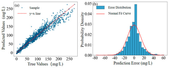
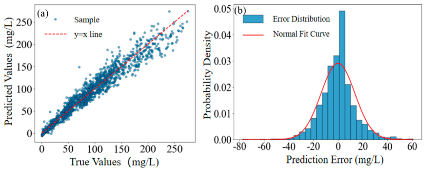
The scatter plot of predicted versus observed values and the residual distribution for the optimized BP-LBFGS model on the test set are shown in Figure 4. The scatter plot shows that data points are tightly distributed on both sides of the diagonal y = x, with good agreement between predicted and observed values across a wide concentration range (0–280 mg/L). However, because samples in the mid-to-low concentration range constitute the vast majority of the dataset, they dominate the global residual statistics and may mask local deviations in the high-concentration range.

Figure 4. The difference between predicted values and true values: (a) scatter plot of predicted values and true values; (b) histogram of prediction errors.

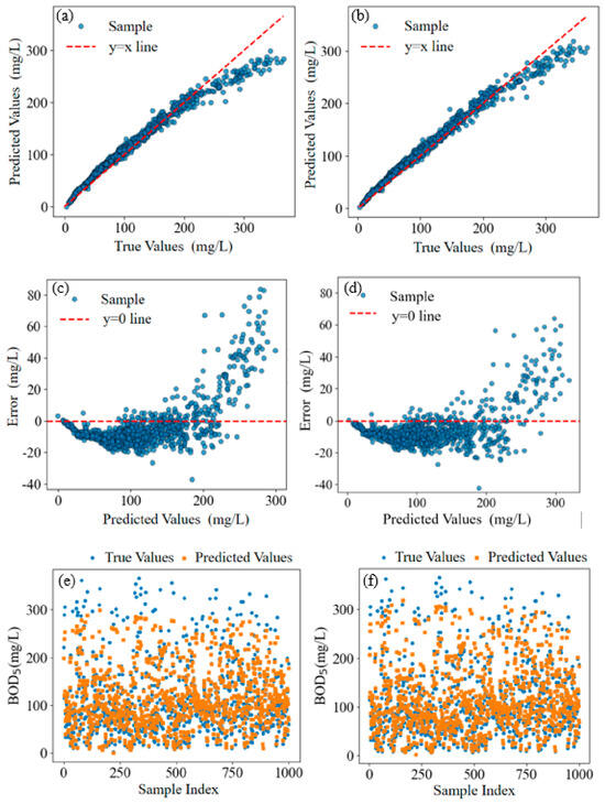
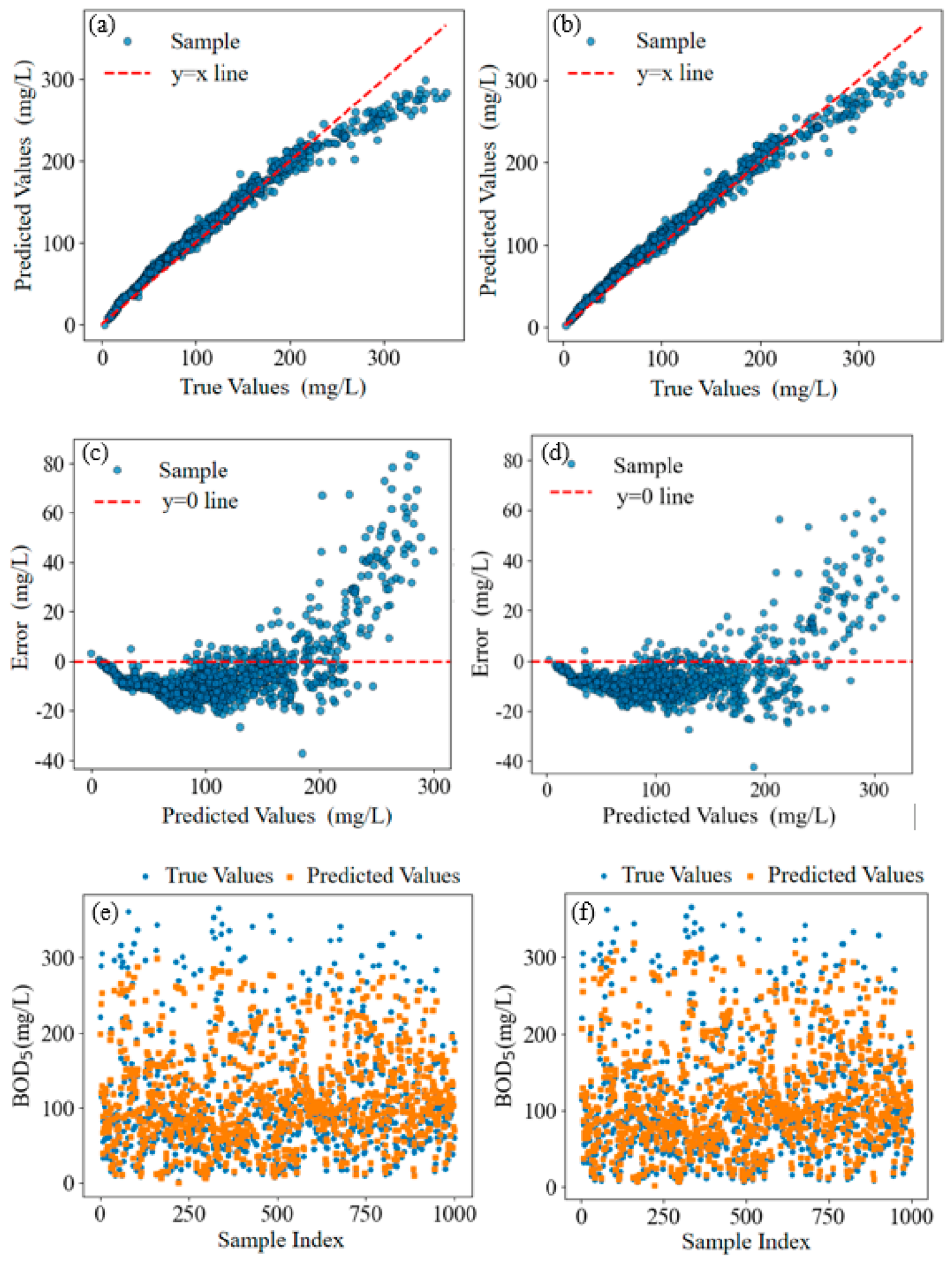
The residual characteristics were further examined on the validation set, with the prediction results shown in Figure 5a,c,e. For BOD₅ concentrations exceeding 250 mg/L, the model exhibits some underestimation. Analysis suggests that high-concentration samples mostly occur under special conditions, such as industrial wastewater admixture or initial stormwater flush of pipe sediments, and such samples constitute a small proportion in the training set, resulting in insufficient model learning. To quantify prediction uncertainty, a bootstrap-based approach was employed. The training data were resampled with replacement 1000 times, and the BP neural network was retrained on each bootstrap sample. The 95% prediction intervals were constructed using the 2.5th and 97.5th percentiles of the bootstrap predictions. On the test set, the resulting 95% prediction interval width averaged ±18.5 mg/L around the point estimate, covering approximately 94.2% of the observed values, indicating well-calibrated uncertainty estimates. For high-concentration samples (>250 mg/L), the interval width increased to ±32.1 mg/L, reflecting the greater prediction uncertainty in this regime. These uncertainty bounds provide practical guidance for decision-makers: when the prediction interval exceeds a regulatory threshold, additional confirmatory sampling is recommended.

Figure 5. Prediction results on the validation set: (a) True values vs predicted values without a piecewise modeling strategy, (b) True values vs predicted values with a piecewise modeling strategy, (c) Residual plot without a piecewise modeling strategy, (d) Residual plot with a piecewise modeling strategy, (e) Difference plot of true values vs predicted values without a piecewise modeling strategy, (f) Difference plot of true values vs predicted values with a piecewise modeling strategy.

To address the prediction deviations in the high-concentration interval, this study further explored the corrective effect of a piecewise modeling strategy. The training set was partitioned into two subsets using 250 mg/L as the threshold: a low-concentration subset (<250 mg/L) and a high-concentration subset (≥250 mg/L), with independent BP neural network models constructed for each subset. The high-concentration model’s hyperparameters were re-optimized via grid search to adapt to its sample distribution. During prediction, the measured input characteristics (e.g., COD) were used to determine the concentration interval, and the corresponding sub-model was invoked. After this piecewise correction, as shown in Figure 5b,d,f, the model achieved an R² of 0.9535 and an RMSE of 16.108 mg/L on the validation set. Following the piecewise modeling correction, R² increased to 0.9700, and RMSE decreased to 12.936 mg/L, effectively suppressing the systematic underestimation tendency in the high-concentration range. It should be noted that while piecewise modeling effectively improved accuracy within the specific interval, the introduced “hard threshold” splitting may reduce the model’s engineering simplicity. In subsequent work, adaptive weighted ensemble strategies or multi-task learning frameworks could be explored to achieve smoother full-range prediction.

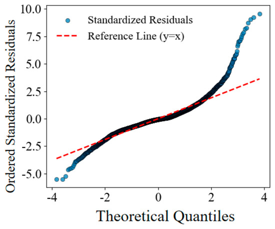
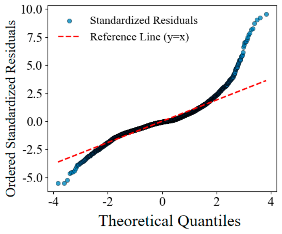
To validate the regression assumptions, the distribution of residuals on the test set was examined. Figure 6 shows the Q-Q plot of standardized residuals against theoretical quantiles. The points closely follow the diagonal line, indicating approximate normality, which is further supported by the histogram in Figure 4b. A Shapiro–Wilk test yielded a p-value of 0.087 (non-significant at α = 0.05), confirming that the residuals do not deviate substantially from normality. This justifies the use of ordinary least-squares-based metrics for model evaluation.

Figure 6. Q-Q plot of standardized residuals against theoretical quantiles.

To more rigorously compare strategies for mitigating the high-concentration underestimation, two additional approaches, SMOTE oversampling and piecewise correction, were implemented. SMOTE generates synthetic high-concentration (BOD₅ ≥ 250 mg/L) samples in the training set to balance the class distribution, while piecewise correction builds separate sub-models for low- and high-concentration zones (threshold = 250 mg/L). Table 6 compares their performance on the validation set. Both methods substantially improve the overall R² (from 0.9535 to ~0.97) and reduce overall RMSE. In the high-concentration segment, SMOTE achieves lower RMSE (18.795 vs. 30.955 mg/L) and MAE (14.586 vs. 27.024 mg/L) than piecewise correction, indicating its superior ability to handle rare extreme samples. However, piecewise correction is simpler to implement and does not alter the original data distribution; it also yields a slightly lower MAPE overall (13.056% vs. 13.661%). Given the comparable overall performance and the ease of implementation, piecewise correction as the final improvement strategy was adopted (Figure 5). Future work may explore ensemble methods that combine both strategies for balanced performance across all concentration ranges.

Table 6. Comparison of the performance on the validation set.

Strategy	Overall R2	Overall RMSE (mg/L)	MAPE (%)	High-Conc. RMSE (mg/L)	High-Conc. MAE (mg/L)
Baseline (no fix)	0.9535	16.108	14.051	46.258	42.902
SMOTE oversampling	0.9699	12.949	13.661	18.795	14.586
Piecewise	0.9700	12.936	13.056	30.955	27.024

3.4. Analysis of Predictive Effectiveness Under Low-Dimensional Features

The results demonstrate that high-accuracy BOD₅ prediction (R² = 0.957) was achieved even under non-temporal conditions using only COD, NH₄⁺-N, and TP, three routinely monitored water quality indices. It suggests that the predictive capability of the proposed model does not rely on high-dimensional inputs, but rather on the strong intrinsic coupling relationships among key biochemical indicators in drainage systems.

Among all, the COD serves as a direct proxy for total organic matter concentration and provides the dominant explanatory signal for BOD₅ variation. NH₄⁺-N reflects nitrogen transformation processes during microbial degradation of organic matter, particularly under anaerobic conditions commonly observed in sewer pipelines. TP, although less directly correlated with organic carbon degradation, captures nutrient-related microbial activity and indirectly reflects system-level biochemical conditions. When combined, these variables provide complementary perspectives on organic pollution dynamics, enabling the model to reconstruct BOD₅ behavior in a data-driven manner.

3.5. Comparison with Existing Studies and Model Implications

Compared with previous studies that used SVR, MARS, or deep learning models, the proposed framework achieves comparable and, in some cases, superior results, as shown in Table 7.

Table 7. Comparison of BOD₅ prediction studies.

Data Source	Samples	Input Features	Best Model	R2	RMSE (mg/L)	MAE (mg/L)	MAPE (%)	Ref.
WWTP, secondary effluent	440 (weekly)	COD, SS, TKN, pH, NO2 (5)	SVR (rbf)	0.464	3.26	2.53	—	[20]
River water	—	pH, EC, DO, WT, COD, SS, T-N, T-P (8)	Deep ESN	0.854	0.054	—	—	[28]
WWTP, effluent	527	12 process variables (RF selected)	GB-LSTM	0.98	2.70	—	8.97	[22]
Drainage network	10,382	COD, NH4+-N, TP (3)	BP-LBFGS	0.961	12.753	7.912	12.89	This study

BOD of the secondary treatment effluent was predicted by SVR with a radial basis function kernel [20]. The R² was 0.464, and RMSE was 3.26 mg/L using five input features selected by random forest. The data were obtained from a weekly monitoring system. Kim et al. developed a Deep Echo State Network (Deep ESN) model for river BOD prediction using eight water quality variables (pH, EC, DO, WT, COD, SS, T-N, and T-P) [28]. An R² of 0.854 and RMSE of 0.054 mg/L were achieved. Wang et al. proposed a gradient boosting LSTM (GB-LSTM) ensemble model for WWTP effluent BOD prediction, and achieved an R² of 0.98 and RMSE of 2.70 mg/L [22]. However, the study employed 12 input features for high accuracy.

In contrast, this study demonstrates that a properly configured BP neural network, combined with feature selection and algorithm optimization, can achieve high predictive accuracy (R² ≈ 0.96) under realistic engineering constraints. This highlights that model complexity is not inherently better; rather, the degree of match between the model and the problem characteristics and practical constraints is the key determinant of performance. The superior performance of the proposed model can be attributed to three factors: (1) the strong intrinsic correlation between COD and BOD₅ in drainage networks (r = 0.976), which provides a robust predictive foundation; (2) the appropriateness of the single-hidden-layer architecture for the relatively low-dimensional input space, avoiding overfitting; and (3) the suitability of the L-BFGS optimizer for the medium-sized dataset (10,511 samples), which offers stable convergence without learning rate tuning. Unlike WWTP-based studies [19,20,28] that benefit from relatively stable influent conditions, the drainage network setting presents greater data heterogeneity, making the achieved R² of 0.957 particularly noteworthy. The temporal models such as LSTM [22] achieve comparable accuracy but require continuous high-frequency monitoring data that is rarely available in practical drainage network operations, underscoring the practical advantage of the proposed non-temporal approach.

3.6. Generalization Limitations and Domain Shift

As shown above, a significant decline in predictive performance was observed when applying the model to external datasets from different regions. The R² decreased from 0.957 (Shenzhen, data used in this study) to 0.844 (Jinan), 0.412 (Hohhot), and 0.164 (Melbourne). It indicates strong distributional shift effects across drainage systems. This can be attributed to two factors, including differences in wastewater composition and industrial discharge structure, and shifts in the COD-BOD₅ relationship across regions.

These results suggest that the proposed model captures region-specific statistical relationships rather than universal physical laws. Therefore, cross-regional deployment requires domain adaptation or transfer learning strategies. In practical applications, a small amount of local calibration data may be sufficient to significantly improve model robustness. From a practical application perspective, the proposed model can be deployed in several scenarios: first, as a real-time BOD₅ estimation tool integrated with existing COD/NH₄⁺-N/TP online sensors in drainage monitoring stations, providing continuous water quality assessment without the 5-day incubation delay; second, as an early warning system for detecting anomalous organic pollution events, where sudden deviations between predicted and observed values (if occasional BOD₅ measurements are available) can trigger targeted investigations; and third, as a planning tool for prioritizing pipeline cleaning and maintenance schedules based on estimated BOD₅ load distribution across the network. For improving accuracy in future studies, several strategies are recommended: (1) transfer learning using small amounts of local calibration data from target regions, which is expected to significantly improve cross-regional performance; (2) adaptive model updating protocols that periodically retrain the model with newly acquired data to track temporal drift in wastewater characteristics; (3) hybrid mechanistic–data-driven frameworks that incorporate hydraulic and biochemical process knowledge as constraints or additional features; and (4) ensemble approaches combining multiple models trained on different data subsets to improve robustness and quantify prediction uncertainty.

4. Conclusions

An interpretable BP neural network model has been developed to predict BOD₅ in urban drainage systems under limited monitoring conditions. In this study, only three water quality indices, COD, NH₄⁺-N, and TP, were used as inputs, and the model achieves high prediction accuracy without relying on temporal information. It demonstrates the feasibility of low-dimensional, data-driven modeling for complex water-quality prediction. It was found that COD was the dominant predictor of BOD₅, while NH₄⁺-N and TP provided supplementary information on wastewater biochemical processes. The model performs well within the training domain but shows a significant decline in performance on cross-regional validation. It indicates strong distributional shifts across drainage systems. Overall, this study provides a simple and interpretable machine learning framework for rapid BOD₅ estimation, while highlighting the challenge of model generalization in heterogeneous urban drainage environments. Regarding generalization, relative errors exhibit a sharp rise across different geographical sites: MAPE increased from 12.89% (test set, Shenzhen) to 35.07% (Jinan) and 58.63% (Hohhot), with the model largely failing on the Melbourne dataset (MAPE = 14.67% but R² = 0.164). This sharp rise indicates that the model captures region-specific statistical relationships rather than universal physical laws, and cross-regional deployment requires local calibration.

References

- Lee, H.E.; Kang, C. A Multi-Method Risk Assessment Framework to Enhancing the Safety of Urban Underground Private Sewage Treatment Systems. Tunn. Undergr. Space Technol. 2026, 168, 107162. [Google Scholar] [CrossRef] [Scilit]
- Pamudji, M.S.; Cheng, K.K.; Yeung, K.L. Mitigating Hydrogen Sulfide Emissions in Urban Drainage Systems: Efficacy of a Malodor-Control Hydrogel. J. Hazard. Mater. 2025, 495, 139107. [Google Scholar] [CrossRef] [Scilit]
- Zhong, H.; Tang, Y.; Yan, H.; Zhang, Y.; Dong, L.; Wang, B. Corrosion of Pipelines in Urban Water Systems: Current Research Status and Future Trends Based on Bibliometric Analysis. J. Water Process Eng. 2023, 56, 104288. [Google Scholar] [CrossRef] [Scilit]
- Chen, H.; Ji, X.; Li, J.; Li, Y.; Zhang, T.; Zhou, W. Microbial Metabolism-Mediated Transformation of Dissolved Organic Matter: Linking Antecedent Dry-Weather Degradation to First-Flush Effects in Urban Wet-Weather Overflows. J. Environ. Chem. Eng. 2026, 14, 120845. [Google Scholar] [CrossRef] [Scilit]
- Kunetz Thomas, E.; Oskouie Ali, K.; Aderangi, N. Prediction of the Potential for Odor Emissions from an Interceptor Sewer System Using a Mathematical Model with Limited Data Yields Useful Results. J. Environ. Eng. 2024, 150, 04024042. [Google Scholar] [CrossRef] [Scilit]
- Wang, Z.; Xu, J.; He, X.; Wang, Y. Analysis of Spatiotemporal Influence Patterns of Toxic Gas Monitoring Concentrations in an Urban Drainage Network Based on IoT and GIS. Pattern Recognit. Lett. 2020, 138, 237–246. [Google Scholar] [CrossRef] [Scilit]
- McKenzie, G.C. Five-Day Biochemical Oxygen Demand; US Geological Survey: Reston, VA, USA, 2003. [Google Scholar]
- Mohamad Noor, S.S.; Saad, N.A.; Mohd Akhir, M.F.; Abd Rahim, M.S. QUAL2K Water Quality Model: A Comprehensive Review of Its Applications, and Limitations. Environ. Model. Softw. 2025, 184, 106284. [Google Scholar] [CrossRef] [Scilit]
- Baek, S.-S.; Ligaray, M.; Pyo, J.; Park, J.-P.; Kang, J.-H.; Pachepsky, Y.; Chun, J.A.; Cho, K.H. A Novel Water Quality Module of the SWMM Model for Assessing Low Impact Development (LID) in Urban Watersheds. J. Hydrol. 2020, 586, 124886. [Google Scholar] [CrossRef] [Scilit]
- Su, J.; Lin, Z.; Xu, F.; Fathi, G.; Alnowibet, K.A. A Hybrid Model of ARIMA and MLP with a Grasshopper Optimization Algorithm for Time Series Forecasting of Water Quality. Sci. Rep. 2024, 14, 23927. [Google Scholar] [CrossRef] [Scilit]
- Guo, X.; Qiu, Y.; Qin, B.; Guo, Z.; Guo, J.; Li, X.; Tian, R.; Kang, J. A Novel Optical-Electrical-Thermal Coupled Model by BP Neural Network Algorithm: Applied to High-Precision Prediction for Key Performance Parameters of Photovoltaic Modules. Sol. Energy Mater. Sol. Cells 2026, 300, 114263. [Google Scholar] [CrossRef] [Scilit]
- Li, X.; Xu, R.; Fan, J.; Zhang, L.; Sun, W.; Kenjeres, S.; Shang, Y.; Yang, W. Evaluation of Multi-Output Machine Learning Models for Predicting Inhaled Particle Deposition in the Human Upper and Central Airway. Powder Technol. 2025, 458, 120924. [Google Scholar] [CrossRef] [Scilit]
- Singh, S.; Parmar, K.S.; Singh, S. The Role of Artificial Neural Networks in Mathematical Modeling: From Single Architecture to Hybrid Frameworks in Environmental System. Appl. Soft Comput. 2026, 198, 115236. [Google Scholar] [CrossRef] [Scilit]
- Huang, Y.; Jin, Y. Real-Time Water Quality Management in Lake Taihu, China: A Machine Learning Application to High-Frequency Time Series. Water Pract. Technol. 2026, 23, 913–935. [Google Scholar] [CrossRef] [Scilit]
- Najah Ahmed, A.; Binti Othman, F.; Abdulmohsin Afan, H.; Khaleel Ibrahim, R.; Ming Fai, C.; Shabbir Hossain, M.; Ehteram, M.; Elshafie, A. Machine Learning Methods for Better Water Quality Prediction. J. Hydrol. 2019, 578, 124084. [Google Scholar] [CrossRef] [Scilit]
- Mahdian, M.; Noori, R.; Saravani, M.J.; Shahvaran, A.R.; Shahmohammad, M.; Gaffney, P.P.J.; Salamattalab, M.M.; Anboohi, M.S.; Hosseinzadeh, M.; Xia, F.; et al. Linking Hypolimnion to Epilimnion in a Stratified Arctic Lake: Machine Learning-Based Estimation of Hypolimnetic Water Quality from Epilimnetic Measurements. Water Res. 2026, 294, 125367. [Google Scholar] [CrossRef] [Scilit]
- Pati, A.K.; Tripathy, A.R.; Nandi, D.; Thakur, R.R.; Pandey, M. Irrigation Water Quality Prognostication: An Innovative Ensemble Architecture Leveraging Deep Learning and Machine Learning for Enhanced SAR and ESP Estimation in the East Coast of India. J. Environ. Chem. Eng. 2025, 13, 116433. [Google Scholar] [CrossRef] [Scilit]
- Zhao, S.; Wang, Q.; An, Z.; Wang, X.; Su, Y.; Li, J.; Wen, G. Water Quality Estimation and Algae Bloom Prediction Using Machine Learning—A Case Study. J. Water Process Eng. 2025, 80, 109161. [Google Scholar] [CrossRef] [Scilit]
- Khoshvaght, H.; Permala, R.R.; Razmjou, A.; Khiadani, M. Factors Influencing the Effectiveness of Machine Learning Algorithms in Predicting Raw Wastewater Characteristics: An Analysis Based on Weekly Field Data. J. Water Process Eng. 2025, 78, 108702. [Google Scholar] [CrossRef] [Scilit]
- Khoshvaght, H.; Permala, R.R.; Razmjou, A.; Khiadani, M. Machine Learning Approaches for Predicting Biochemical Oxygen Demand and Ammonium Nitrogen: A Decade-Long Weekly Field Study at a Full-Scale Water Resource Recovery Facility. Eng. Appl. Artif. Intell. 2026, 172, 114349. [Google Scholar] [CrossRef] [Scilit]
- Qambar, A.S.; Khalidy, M.M.A. Prediction of Municipal Wastewater Biochemical Oxygen Demand Using Machine Learning Techniques: A Sustainable Approach. Process Saf. Environ. Prot. 2022, 168, 833–845. [Google Scholar] [CrossRef] [Scilit]
- Wang, X.; Wang, J.; Wang, B.; Wei, W.; Zhang, F.; Huang, M.; Liu, H. Enhancing Effluent Biochemical Oxygen Demand Prediction in Wastewater Treatment Plants: An Ensemble Model of Gradient Boosting and LSTM. J. Environ. Chem. Eng. 2025, 13, 117897. [Google Scholar] [CrossRef] [Scilit]
- Pritsis, S.; Clemens-Meyer, F.; Kerger, S.; Legge, A.; Wang, M.; Rokstad, M.M.; Tscheikner-Gratl, F. A Review of Monitoring Site Selection Methods for Urban Drainage Networks—The Missing Link between Theory and Practice. Struct. Infrastruct. Eng. 2026, 1–18. [Google Scholar] [CrossRef] [Scilit]
- Hornik, K.; Stinchcombe, M.; White, H. Multilayer Feedforward Networks Are Universal Approximators. Neural Netw. 1989, 2, 359–366. [Google Scholar] [CrossRef] [Scilit]
- Liu, D.C.; Nocedal, J. On the Limited Memory BFGS Method for Large Scale Optimization. Math. Program. 1989, 45, 503–528. [Google Scholar] [CrossRef] [Scilit]
- Kingma, D.P.; Ba, J. Adam: A Method for Stochastic Optimization. In Proceedings of the International Conference on Learning Representations (ICLR), San Diego, CA, USA, 7–9 May 2014. [Google Scholar]
- Sutskever, I.; Martens, J.; Dahl, G.; Hinton, G. On the Importance of Initialization and Momentum in Deep Learning. In Proceedings of the Proceedings of the 30th International Conference on International Conference on Machine Learning, JMLR.org, Atlanta, GA, USA, 16 June 2013; Volume 28, pp. III-1139–III-1147. [Google Scholar]
- Kim, S.; Alizamir, M.; Zounemat-Kermani, M.; Kisi, O.; Singh, V.P. Assessing the Biochemical Oxygen Demand Using Neural Networks and Ensemble Tree Approaches in South Korea. J. Environ. Manag. 2020, 270, 110834. [Google Scholar] [CrossRef] [Scilit]
Disclaimer/Publisher’s Note: The statements, opinions and data contained in all publications are solely those of the individual author(s) and contributor(s) and not of MDPI and/or the editor(s). MDPI and/or the editor(s) disclaim responsibility for any injury to people or property resulting from any ideas, methods, instructions or products referred to in the content. |
© 2026 by the authors. Licensee MDPI, Basel, Switzerland. This article is an open access article distributed under the terms and conditions of the Creative Commons Attribution (CC BY) license.