


Abstract
Flood occurrence in tropical regions is intensifying due to climate variability and land-use change, increasing the need for reliable flood response time estimation. Accurate prediction of flood lag time (TL)—the interval between the centroid of excess rainfall and peak runoff—is critical for flood early warning and water resource planning. However, TL estimation remains challenging in data-scarce regions because of complex interactions among watershed morphology, rainfall characteristics, and runoff generation processes. This study evaluates four machine learning (ML) algorithms—Random Forest (RF), Artificial Neural Network (ANN), Extreme Gradient Boosting (XGBoost), and Support Vector Machine (SVM)—for predicting TL across twenty gauged watersheds in the Blue Nile Basin of Ethiopia. Fourteen physiographic and hydro-climatic watershed characteristics were used as predictors. Among the tested models, XGBoost achieved the highest training performance (R2 = 0.98, NSE = 0.96), while RF showed better generalization in the test dataset (R2 = 0.77, NSE = 0.70, KGE = 0.71). SVM produced the lowest prediction errors (MAE = 0.95; RMSE = 2.25) but had lower explanatory power (R2 = 0.49). To enhance interpretability and practical applicability, ML-based feature importance was used to develop a parsimonious empirical model: TL = 0.8 + 0.011A − 0.023RI, where A is watershed area and RI is rainfall intensity. This model explained 51% of TL variability and retained much of the predictive skill of more complex ML models. The proposed hybrid ML–empirical framework provides a transparent and operational approach for flood response time estimation in tropical highland watersheds. Its broader applicability remains subject to additional watershed-level validation and regional calibration.
1. Introduction
Tropical regions are characterized by high intensity, short-duration rainfall, strong hydro-climatic seasonality, rapid soil moisture transitions, steep terrain, and high evapotranspiration. These interacting controls coupled with extensive land-use change promote rapid runoff generation and dynamic hydrological connectivity between hillslopes and channels, resulting in short flood lag times [1]. In humid and sub-humid tropical highlands, including the Ethiopian Highlands, runoff generation is frequently dominated by saturation-excess and shallow subsurface flow processes rather than infiltration-excess mechanisms [2,3,4,5,6]. Such process regimes generate highly variable flood lag times and amplify surface erosion and peak flow sensitivity [1].
Under ongoing climate change and accelerating land-use transformation, flood frequency and magnitude in tropical regions are increasing [7]. These changes heighten the importance of accurately estimating watershed response timing—particularly lag time (TL) and time of concentration (TC)—which are essential for flood forecasting, hydraulic infrastructure design, and watershed management [8]. TL is defined as the time interval between the centroid of effective rainfall and the peak discharge at the watershed outlet, representing the delay between rainfall input and watershed response. In contrast, TC is the time required for a water particle to travel from the hydraulically most distant point in the watershed along the longest flow path to the outlet, indicating the time at which the entire watershed contributes to runoff. Although conceptually different, these parameters are closely related, and TC is commonly estimated from TL using empirical relationships (e.g., TC ≈ 1.67 TL) [9,10,11]. In conventional empirical methods, both parameters are commonly estimated primarily from watershed static geomorphologic properties [10]. Because TL can be derived directly from observed rainfall–runoff events and better reflects event-scale watershed response, this study focuses on TL, while TC is discussed only for conceptual comparison and consistency with existing hydrological practice.
However, a growing body of hydrological research suggests that response timing is not solely a fixed watershed attribute but an emergent property of interacting rainfall, storage, and connectivity dynamics [12,13]. Event-scale TL varies with rainfall intensity, antecedent soil moisture, vegetation cover, and the expansion or contraction of saturated source areas [14,15]. In tropical highlands, seasonal shifts in soil moisture and biomass during monsoon transitions significantly alters runoff pathways and response timing [15]. This dynamic behavior challenges the validity of single-valued TC assumptions, a concern echoed in international hydrological discussions emphasizing the inadequacy of fixed empirical formulations in tropical and subtropical systems [16,17].
Despite these insights, TL and TC estimation in humid and sub-humid tropical highlands including Ethiopia continues to rely heavily on empirical formulas developed for temperate watersheds, such as the Kirpich equation and regression-based relationships embedded in the ERA Drainage Design Manual [18]. These formulations were derived from small temperate catchments dominated by infiltration-excess (Hortonian) runoff with relatively stable rainfall–runoff responses due to less pronounced seasonal variability [19,20]. Evidence from the U.S. suggests that during extreme storms, TL becomes more stabilized due to dominant overland flow pathways, enhancing hydrological predictability [21]. However, when such equations are transferred to tropical catchments which are largely governed by saturation-excess runoff processes, substantial predictive bias arises [2,3,4,5]. For instance, recent evaluation studies report large errors in TL and TC estimation, with peak discharge misestimation exceeding 70% in some cases [14,22,23]. These discrepancies reflect a structural mismatch between assumed runoff mechanisms and actual process controls.
Physically based hydrological models attempt to represent infiltration, storage, and routing processes explicitly, yet in Ethiopia, their application remains constrained by sparse hydro-meteorological data and uncertainty in parameterization [24]. Equifinality and calibration challenges further limit their operational reliability in data-scarce tropical environments [25]. Consequently, there is a growing interest in data-driven, context-specific approaches capable of extracting hydrological information directly from observations without requiring fully specified process representations [15]. Recent advances in machine learning (ML) have demonstrated strong skill in modeling nonlinear rainfall–runoff relationships and event-scale hydrological dynamics [26,27,28,29,30]. However, ML models are frequently criticized as “black boxes” with limited interpretability and high data demands, raising concerns about their scientific value and operational applicability [31,32,33]. Deep learning (DL) has further advanced data-driven hydrological modeling by enabling the representation of complex nonlinear and temporally dependent rainfall–runoff relationships. Recent studies have applied bidirectional long short-term memory (BiLSTM) models to flood and streamflow forecasting, demonstrating improved multi-step prediction and the ability to capture temporal dependencies [34,35]. Integrated and hybrid DL architectures have also been developed for streamflow forecasting, including attention-based networks and CNN-GRU/CNN-LSTM models, which combine complementary feature-extraction and temporal-learning capabilities [36,37,38]. Recent reviews further document the rapid development of recurrent, convolutional, attention-based, encoder–decoder, Transformer, physics-guided, and other hybrid DL approaches in hydrology and water resources [39]. However, the performance of these increasingly complex models depends substantially on the availability, quality, and temporal resolution of training data, which can be limiting in data-scarce tropical watersheds.
Recent hydrological scholarship further suggests that ML can reveal process-relevant information embedded in hydrological datasets that may not be readily captured by conventional empirical formulations [40,41]. This distinction between using learning algorithms primarily for prediction and using them to support scientific discovery is particularly important in hydrology, where feature importance can provide interpretable and testable insights into dominant controls [42]. Thus, rather than treating ML solely as a predictive tool, it can also serve as a diagnostic framework for identifying physically meaningful and scale-dependent controls on hydrological response.
Hybrid approaches that integrate ML-derived insights with simplified empirical formulations offer a means of combining predictive performance with process interpretability [43,44,45,46,47]. For instance, ref. [48] demonstrated the value of integrating ML-based reconstruction of sparse suspended sediment concentration (SSC) observations with process-based watershed simulation in a data-scarce environment. Similarly, ref. [33] improved flood-peak arrival-time prediction through feature engineering and ensemble learning, while refs. [31,49] showed that ML-informed regression approaches can improve predictive accuracy while retaining interpretability. Such approaches are particularly relevant to data-scarce tropical basins, where model transparency, data efficiency, and operational applicability are critical.
In tropical data-scarce regions, including Ethiopia, ML-based hydrological studies remain limited and often emphasize prediction rather than interpretation. Existing studies have demonstrated the predictive potential of Random Forests, XGBoost, and neural networks for streamflow, flood susceptibility, and erosion modeling [43,50,51]. However, these studies typically focus on individual watersheds and predefined predictor sets. Consequently, limited attention has been given to identifying the dominant controls of event-scale response timing across multiple heterogeneous watersheds and translating data-driven insights into simple, physically interpretable formulations.
This study advances hydrological understanding by reframing lag time estimation from a purely empirical scaling exercise to a diagnostic investigation of dominant process controls in tropical watersheds. Instead of limiting our analysis solely to model performance comparison, we use ML as an exploratory and interpretative tool to identify the primary physiographic and rainfall drivers governing event-scale TL variability across twenty watersheds spanning multiple climatic zones of the Blue Nile Basin in Ethiopia. Specifically, the novelty of this contribution lies in four key aspects: (i) the process-informed diagnostic use of ML, positioning learning algorithms as tools for hydrological inference rather than purely predictive instruments; (ii) multi-watershed and multi-climatic validation, enabling assessment of dominant TL controls across heterogeneous tropical highland environments; (iii) systematic translation of ML-derived feature importance into a parsimonious two-parameter empirical model, thereby bridging data-driven discovery with operational hydrological practice; and (iv) development of an interpretable, regionally calibrated framework for flood response-time estimation that offers practical potential for data-limited tropical watersheds and provides a basis for further regional validation and operational application. By linking data-driven modeling with hydrological reasoning, the framework strengthens the connection between predictive analytics and process-based understanding. Because the present dataset comprises 20 gauged watersheds within the Upper Blue Nile Basin, transferability beyond the sampled watersheds remains to be established.
Building on this framework, we test the hypotheses that (i) lag time in tropical highland watersheds is governed by a small subset of physically interpretable predictors whose influence varies across events and climatic zones and (ii) ML-based feature importance can be systematically translated into a parsimonious empirical formulation that preserves predictive skill while enhancing interpretability and operational applicability. Accordingly, the objectives of this study are to (i) evaluate and identify the best-performing ML algorithms for lag-time (TL) estimation and (ii) develop an ML-informed parsimonious hybrid model that balances predictive accuracy with operational practicality in data-limited settings. Ultimately, this approach contributes to a deeper process-based understanding of event-scale hydrological response while delivering a practical tool for improved flood response time forecasting.
2. Materials and Methods
2.1. Study Sites
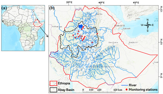
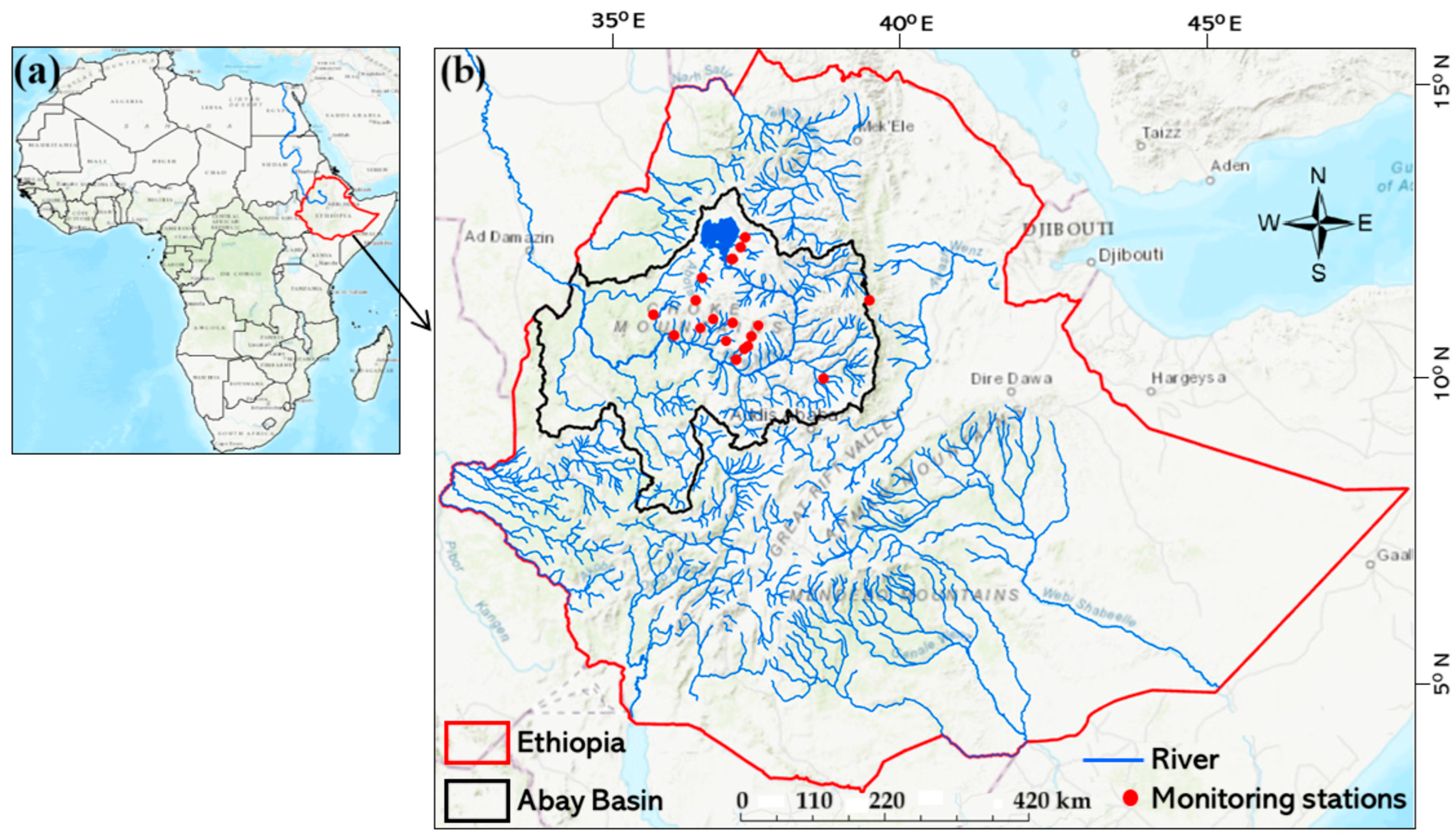
This study was conducted in twenty gauged watersheds within the Upper Blue Nile Basin (also known as the Abay Basin), a region that represents diverse tropical highland hydrological environments (Figure 1, Table S1). The basin experiences warm conditions with distinct wet and dry seasons, with most rainfall occurring during the Kiremt season (May–October). Annual precipitation varies widely—from less than 1000 mm (Lat 10.7775°; Long 36.285278°) to more than 2454 mm (Lat 11.001944°; Long 36.940833°)—and is characterized by strong interannual variability. The topography is highly complex, with mean elevations ranging from 1572 to 3251 m (Table S1), encompassing steep slopes, rolling hills, and deeply incised valleys that strongly influence runoff generation and flood dynamics. The basin contributes more than 60% of the Nile River’s total flow, originating from the Ethiopian highlands, which span climates from humid in the southwest to semi-arid in the northeast.
Figure 1.
Locations of twenty tropical highland watersheds in the Upper Blue Nile Basin (Abay Basin), Ethiopia, showing rivers (blue), monitoring stations (red dots), basin boundary (black), and national boundary (red). (a) shows the location of the study area in Africa, while subfigure (b) provides a detailed view of the study area, showing the spatial distribution of the selected watersheds and their monitoring stations within the Upper Blue Nile Basin.
Land degradation driven by poor land management practices has resulted in severe soil erosion, threatening agricultural productivity, degrading aquatic ecosystems, and reducing the lifespan of downstream reservoirs [24]. Soils are predominantly clay and loam with variable infiltration capacity. Land cover is dominated by rain-fed agriculture, interspersed with rural settlements and patches of natural vegetation.
These heterogeneous biophysical conditions promote rapid hydrological responses to rainfall, often leading to flash flooding, making the selected watersheds particularly suitable for investigating flood response times and associated hydrological processes.
2.2. Data Collection and Processing
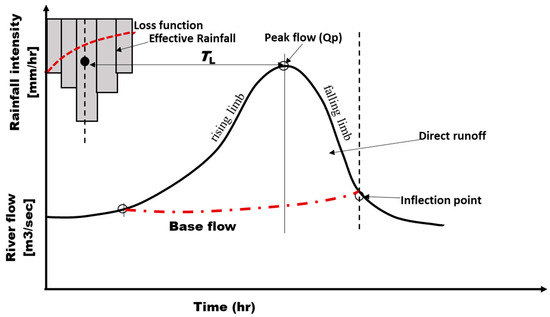
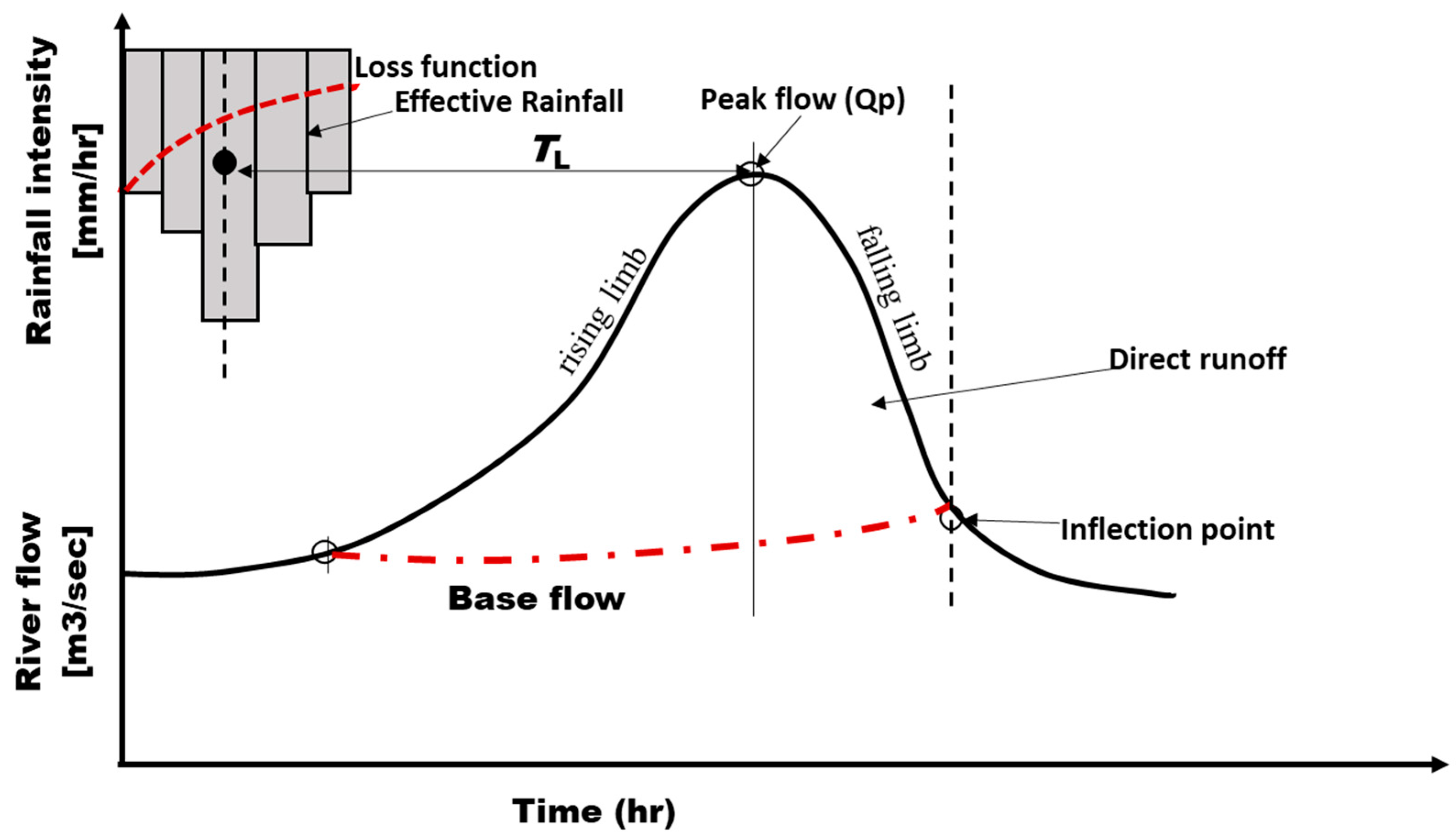
Rainfall and runoff data were obtained from 2014–2024 through collaborations with KAKENHI, SATREPS, WLRC, FEWS and local universities (see Table S1 for details). Lag time (TL) for each storm event was defined as the interval between the centroid of excess rainfall and the peak discharge [20,52] (Figure 2). Excess rainfall was estimated using an event-specific φ-index to account for infiltration losses and determine the effective-rainfall hyetograph. Direct event runoff was obtained by separating baseflow from the total streamflow using the Web-based Hydrograph Analysis Tool (WHAT) [53]. Baseflow was separated using the Eckhardt recursive digital filter implemented in WHAT, with the parameter settings specified for the corresponding streamflow conditions. For each retained event, the φ-index was determined separately by iteratively adjusting the constant infiltration rate until the cumulative rainfall excess equaled the observed direct-runoff depth. Rainfall and discharge records were temporally aligned, and only events with concurrent and sufficiently complete observations were retained; incomplete or unsuitable events were excluded. The rainfall gauge/data source and monitoring period for each watershed are provided in Supplementary Table S1. The centroid of effective rainfall was computed as the weighted average time of the effective rainfall hyetograph:
where Wi is rainfall depth in period i, ti time of interval i, and n is the number of 10 min intervals in the event. Lag time (TL) was then calculated as the time difference between the centroid of effective rainfall and the corresponding peak discharge of the direct runoff hydrograph (Figure 2). To ensure event independence, rainfall–runoff events were selected following the criteria of [54,55,56]. Only isolated storm events producing a single, well-defined hydrograph peak followed by an uninterrupted recession limb were retained. Multi-peaked hydrographs and consecutive rainfall events were excluded to minimize overlap between successive runoff responses and to ensure that each selected event represented an independent rainfall–runoff event. Consequently, a total of 302 independent rainfall–runoff events were retained, with each watershed contributing between 6 and 22 events for subsequent analysis. Hyetographs and hydrographs were constructed in Microsoft Excel (2020). Figure 2 illustrates the derivation of TL.
Figure 2.
Conceptual diagram illustrating how TL is derived from hyetographs and hydrographs based on definitions from [20].
2.3. Predictor Variables
Twenty watershed descriptors were initially identified from the literature [57]. Fourteen were retained for modeling based on data completeness, measurement accuracy, and hydrological significance. These variables represented morphometric properties (e.g., watershed area, slope, drainage density, circularity ratio, and perimeter), hydraulic characteristics (e.g., stream length, relief, elevation, and channel slope), hydrologic properties (e.g., Curve Number), and rainfall attributes (e.g., mean effective-rainfall intensity [RI = total effective rainfall/event duration], duration, depth, and mean annual precipitation). For analysis, predictors were grouped into four categories [14,20]: (i) watershed size, (ii) slope characteristics, (iii) flow resistance, and (iv) rainfall input. Spatial features were extracted from 12.5 m resolution DEMs, while land-use and soil data were derived from remote sensing and validated through field surveys.
2.4. Machine Learning Model Setup
To predict flood lag time (TL), we implemented four machine learning (ML) algorithms—Random Forest (RF), Artificial Neural Networks (ANN), Extreme Gradient Boosting (XGBoost), and Support Vector Machines (SVM)—because of their proven capability to model complex nonlinear hydrological processes [26]. The models were trained to learn the relationships between watershed physiographic and climatic descriptors (Section 2.3) and observed TL values.
Prior to model development, a fixed random seed (set.seed = 123) was specified to ensure full reproducibility of data partitioning, hyperparameter optimization, and model training. The dataset was stratified into 80% training and 20% testing subsets using the create Data Partition function in the caret package, thereby preserving the distribution of observed lag-time values between the two subsets. Several train–test ratios (70/30, 75/25, and 80/20) were initially evaluated, and the 80/20 split provided the most balanced predictive performance while maintaining sufficient data for both model calibration and independent evaluation.
Hyperparameter optimization was performed exclusively on the training dataset using internal cross-validation, while the testing dataset was reserved solely for final model evaluation. Random Forest was optimized using 10-fold grid-search cross-validation over the mtry, splitrule, and min.node.size parameters. SVM and XGBoost were optimized using 5-fold cross-validation, where the cost and gamma parameters were tuned for SVM, and nrounds, max_depth, etc., gamma, subsample, colsample_bytree, and min_child_weight were optimized for XGBoost. Following hyperparameter optimization, each algorithm was retrained using the optimal parameter combination before independent testing. Predictor variables were normalized for ANN and SVM because these algorithms are sensitive to differences in variable scale, whereas RF and XGBoost were trained using the original predictor values because tree-based algorithms are inherently insensitive to predictor scaling.
Final configurations were:
- RF: 500 trees with permutation-based variable importance (Figure S2);
- ANN: Two hidden layers with normalized predictors;
- XGB: Optimized using 100 boosting rounds, with RMSE as the optimization metric;
- SVM: Radial basis function (RBF) kernel with normalized predictors.
Each algorithm extracts information from the predictor variables differently:
2.4.1. Random Forest (RF)
RF is an ensemble method that builds multiple decision trees using bootstrap samples and random feature subsets. Trees split the data into increasingly homogeneous groups of watershed and rainfall attributes, minimizing prediction error. The final TL prediction is the average of all trees, and variable importance is quantified by the reduction in impurity or accuracy decrease when predictors are permuted.
2.4.2. Support Vector Machine (SVM)
Support Vector Regression (SVR), a variant of SVM, maps predictors into a high-dimensional feature space using kernel functions. A regression hyperplane is then fitted to minimize prediction error within a defined margin (ε-insensitive loss). This allows the model to capture nonlinear relationships between watershed descriptors and TL while maintaining strong generalization on small or noisy datasets.
2.4.3. Artificial Neural Networks (ANNs)
ANNs are composed of interconnected layers of neurons that apply linear transformations followed by nonlinear activation functions. By propagating inputs through two hidden layers, the network learns complex nonlinear interactions among watershed and rainfall variables. The model iteratively adjusts connection weights through backpropagation to minimize error between predicted and observed TL.
2.4.4. Extreme Gradient Boosting (XGBoost)
XGBoost is an advanced gradient boosting algorithm that sequentially builds decision trees, where each new tree focuses on correcting residual errors from the previous ensemble. Using the RMSE-based objective function, XGBoost efficiently identifies nonlinear and high-order interactions among predictors, making it effective for capturing complex hydrological processes such as TL dynamics.
This modeling framework allowed us to assess how different ML strategies translate physiographic and climatic information into TL predictions while also comparing predictive performance across algorithms.
2.5. Model Performance Evaluation
Performance was assessed using seven standard hydrological metrics: coefficient of determination (R2), Nash–Sutcliffe Efficiency (NSE), Percentage Bias (PBIAS), Root Mean Square Error (RMSE), Mean Absolute Error (MAE), Kling–Gupta Efficiency (KGE), and the ratio of RMSE to the standard deviation of observations (RSR). Formulas followed standard hydrological modeling practice, where is the measured TL, is the mean measured TL, is the simulated TL, and is the average simulated TL.
where r is Pearson’s correlation, β is the bias ratio (μS/μO), and γ is the variability ratio (CVS/CVO).
2.6. ML-Informed Hydrological Response Time Modeling
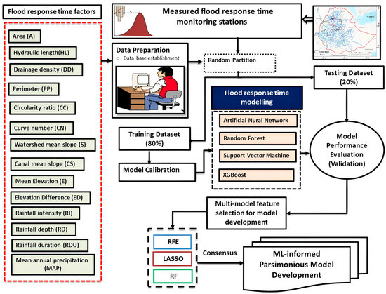
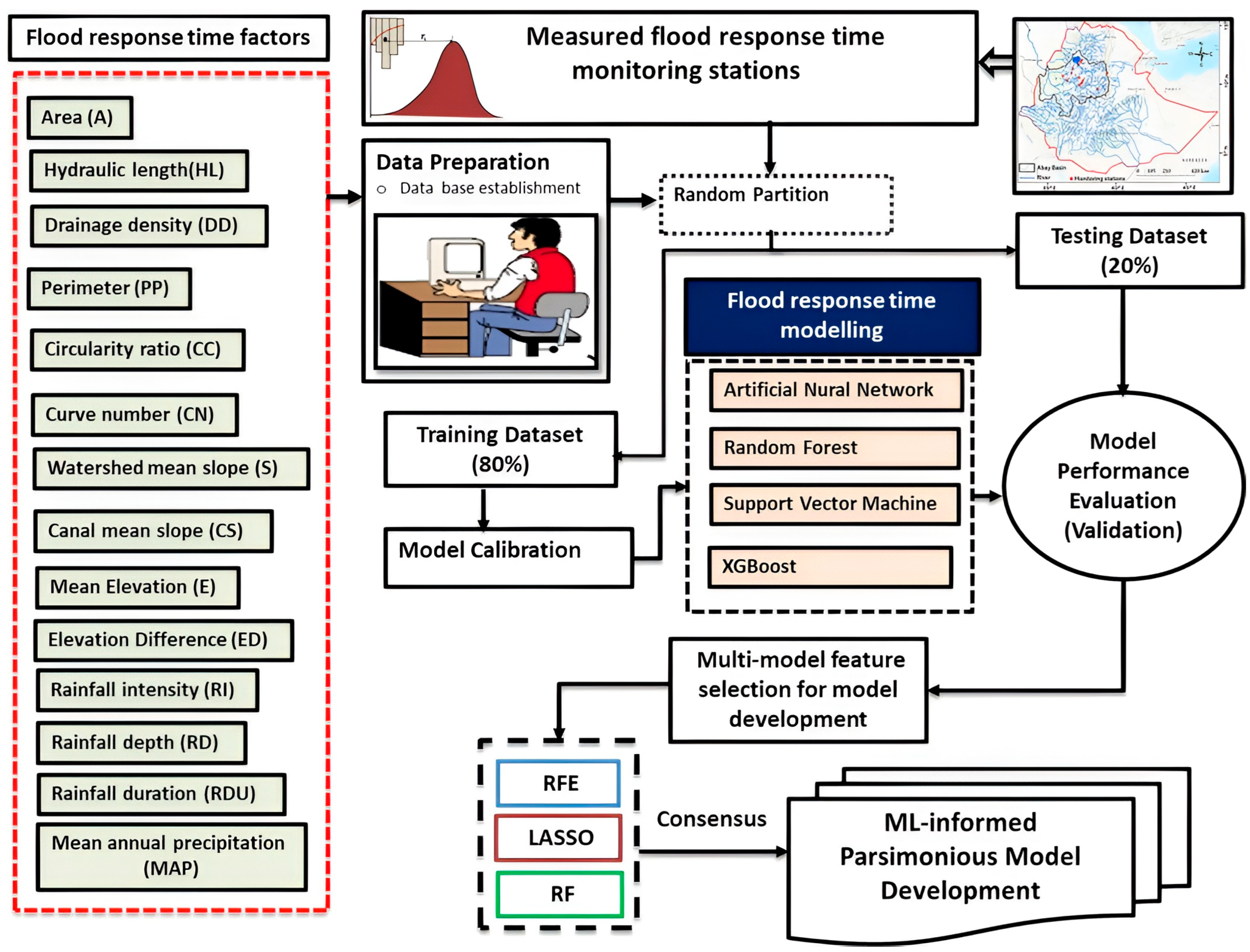
To improve computational efficiency, a simplified empirical regression model for TL was developed using predictors identified by machine learning-based feature selection [50,58]. We employed well-established techniques to enhance model stability and interpretability by removing redundant features [59]. Three techniques—Recursive Feature Elimination (RFE), Least Absolute Shrinkage and Selection Operator (LASSO), and Random Forest importance—were applied (Figure 3). Each approach has its own particular strengths [59]. Recursive Feature Elimination (RFE) is a wrapper-based feature selection technique that iteratively identifies the most predictive subset of variables. Starting with the complete set of features, a model is fitted and feature importance scores are computed. The least important feature is removed, and the procedure is repeated until the specified number of predictors remains. This process ensures the final subset maximizes model accuracy while minimizing redundancy and noise [59,60,61]. In contrast, the Least Absolute Shrinkage and Selection Operator (LASSO) is a linear regularization method that performs variable selection by penalizing the absolute magnitude of regression coefficients and enhances interpretability by introducing an L1 penalty to the loss function. This L1 penalty is controlled by a regularization parameter λ. This penalty forces some coefficients to shrink exactly to zero, effectively eliminating irrelevant predictors and retaining only the most informative variables, thereby enhancing model interpretability and reducing overfitting [59,61,62]. Mathematically, the LASSO objective function is defined as:
where
minimize β: 1/(2 × N) × ||Y − Xβ||2 + λ × ||β||1
Figure 3.
Diagram depicting the detailed methods used for the present study.
- N is the number of observations;
- Y is the vector of observed data;
- X is the input features matrix;
- β represents the regression coefficients (to be estimated);
- ||.|| denotes the L2 norm (Euclidean norm) of a vector;
- ||β||1 is L1 norm of the vector β (sum of the absolute values of β);
- λ ≥ 0 is the regularization parameter controlling the strength of the penalty.
By zeroing out irrelevant coefficients, LASSO simplifies the model and retains only the most informative features, enhancing interpretability and performance.
Random Forest Feature Importance is a model-based feature selection method that estimates the relevance of each variable using an ensemble of decision trees. In this approach, feature importance is quantified by measuring the average reduction in node impurity (e.g., Gini impurity for classification or variance for regression) or prediction error when a feature is used to split the data across all trees in the forest [63]. This method inherently accounts for nonlinear relationships and interactions between variables, making it well-suited for high-dimensional and complex datasets. The importance score for a given feature i can be calculated as:
Once these scores are computed, features are ranked according to their importance. The top-ranked variables are typically retained for further modeling or analysis, as they contribute most significantly to the predictive performance of the Random Forest model.
A consensus-based approach [49,64] was adopted, retaining predictors selected by at least two methods (Figure 3). This criterion was used to improve the robustness of feature selection by identifying predictors consistently supported across complementary algorithms rather than relying on any single method. Because RFE, LASSO, and Random Forest importance differ in their selection principles, variations in variable rankings are expected. Therefore, selection by multiple methods should not be interpreted as evidence of greater physical importance but rather as an indication of greater methodological consistency. The selected predictors were subsequently used to develop a parsimonious multiple linear regression model. We acknowledge that alternative consensus thresholds or stability-selection approaches could produce different predictor sets and should be evaluated in future studies using larger datasets. To systematically assess multicollinearity among the candidate predictors, we calculated the Variance Inflation Factor (VIF) for each predictor variable. VIF quantifies how much the variance of a regression coefficient is inflated due to correlations with other predictors, with values exceeding 10 indicating problematic collinearity and values between 5 and 10 suggesting moderate concerns (see details in Supplementary Material, Table S3). The regression model was calibrated on 80% of the data and validated on 20%. Performance was evaluated with RMSE and R2, and observed–predicted scatterplots. The final regression equation was saved as an RDS file for reproducibility and operational use in R studio version 2024.12.1+563 (“Kousa Dogwood”).
3. Results and Discussion
3.1. Correlation Analysis
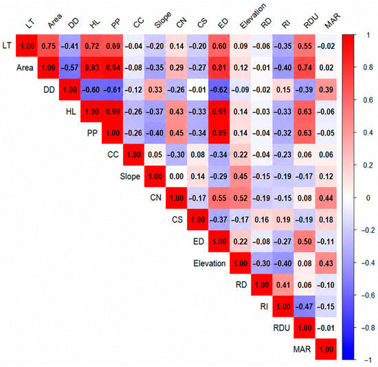
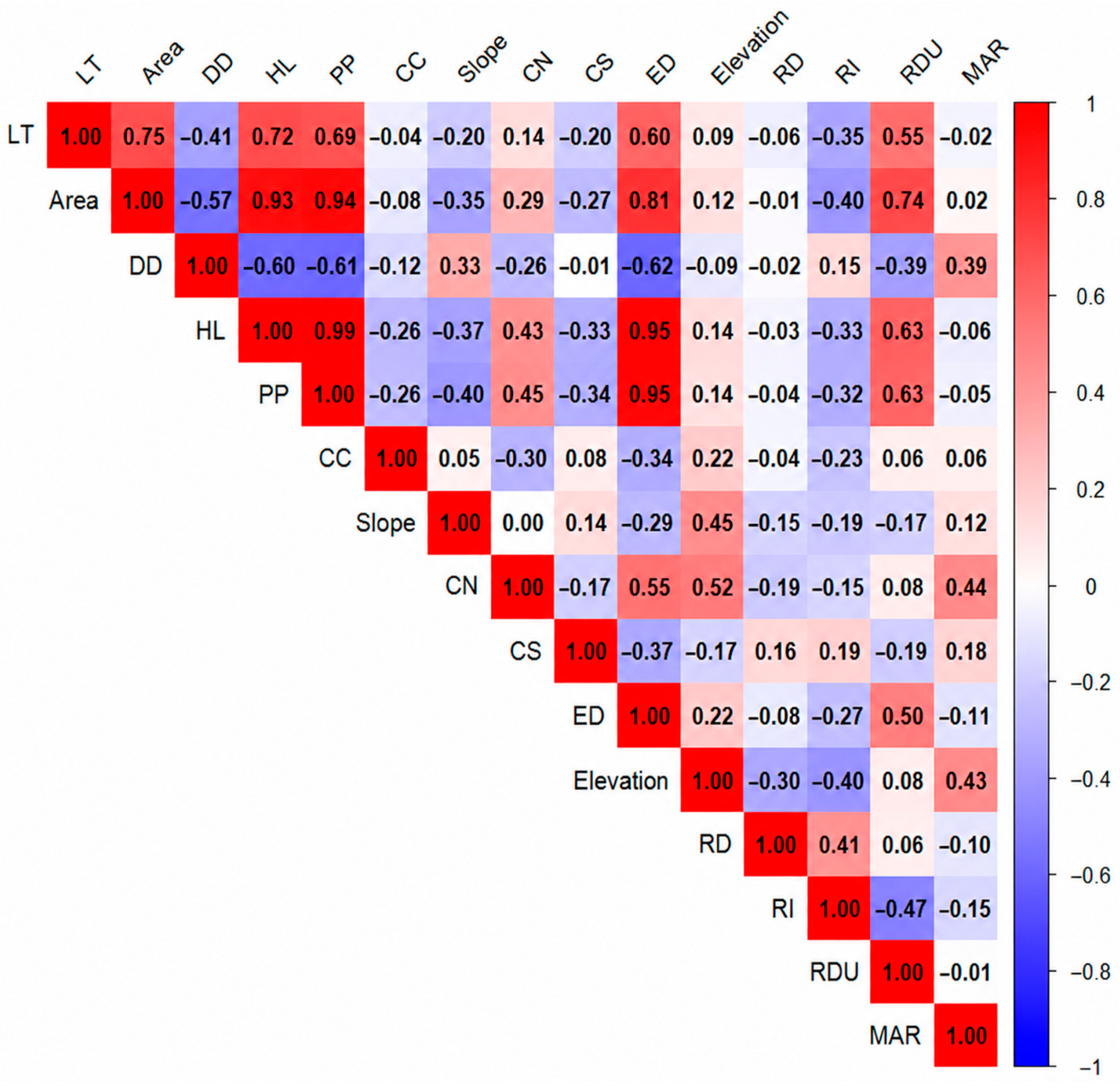
The correlation analysis (Figure 4) revealed that watershed morphometric characteristics are the dominant controls on TL. A (r = 0.75) and HL (r = 0.69) exhibited strong positive correlations with TL, indicating that larger catchments with longer flow paths experience delayed runoff responses. Area also covaried strongly with PP and HL (r > 0.85), confirming that catchment scale simultaneously governs boundary size and channel length, while its negative correlation with DD (r ≈ –0.55) suggests that larger basins tend to have less dense channel networks, further extending lag times. A recent global review by [57] supports these findings, showing that more than 25 empirical equations worldwide use basin area as a key predictor of lag time. The relationship was strong and nearly linear in micro-watersheds but weakened at larger scales due to greater heterogeneity in physical characteristics, increased drainage network complexity, diverse hydrological processes, and spatial variability in rainfall distribution.
Figure 4.
Correlation matrix of lag time (TL) with watershed physiographic and climatic variables.
Climatic indices exerted more pronounced effects. RI (r = –0.55) showed a strong negative correlation with TL, indicating that high-intensity storms accelerate runoff and shorten watershed response times. RI was also inversely correlated with RDU (r ≈ –0.45) and elevation (r ≈ –0.40), suggesting that short, intense storms frequently occur in steep, high-elevation catchments, thereby promoting faster hydrologic responses. In contrast, RDU exhibited only a weak negative relationship with TL (r = –0.15), implying that storm length alone does not substantially prolong lag time once soils are saturated. Similarly, ref. [65] reported that TL is inversely proportional to rainfall intensity, with a moderate correlation (r = –0.41, R2 = 0.17), based on 95 rainfall–streamflow events in the Selangor River Basin, Malaysia. They attributed the moderate relationship to complex interactions with other hydrological variables. More recently, ref. [66] introduced a multivariate framework incorporating threshold strength (T) and diagonality (D) to quantify threshold-mediated runoff responses. Their study demonstrated that runoff behavior is shaped jointly by rainfall amount and intensity, and that these thresholds vary substantially among sub-watersheds depending on physical characteristics such as slope and imperviousness.
3.2. Performance of Machine Learning Algorithms
Four machine learning (ML) algorithms (RF, XGB, ANN, and SVM) were evaluated for flood lag time (TL) prediction using an 80/20 train–test split. Model performance was assessed with R2, NSE, KGE, MAE, RMSE, PBIAS, and RSR (Table 1).
Table 1.
Flood response time model prediction performance measure results using four ML algorithms; R2, KGE, MAE, RMSE, PBIAS, RSR and NSE.
The training phase revealed stark differences in model fit. XGB achieved the highest accuracy (R2 = 0.98, NSE = 0.96, MAE = 0.64), followed by RF (R2 = 0.76, NSE = 0.77). In contrast, ANN and SVM showed moderate correlation-based performance (R2 = 0.66) but exhibited large discrepancies in bias-related metrics. These differences highlight that individual performance indicators capture different aspects of model behavior and should be interpreted together rather than independently.
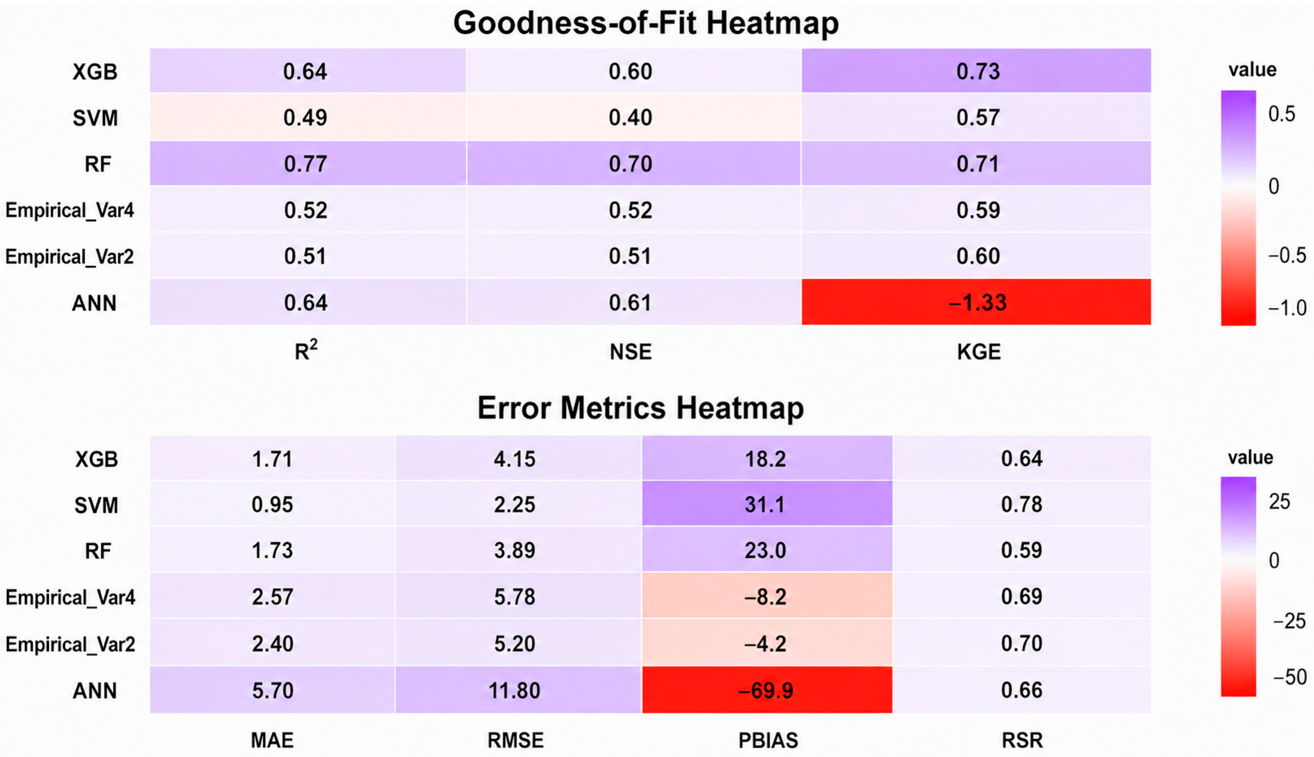
During testing, RF emerged as the most robust and best-generalizing model, achieving the highest R2 (0.77) and NSE (0.70), a strong KGE (0.71), and the lowest RMSE (3.89). While XGB’s testing metrics (R2 = 0.64, NSE = 0.60) confirmed a significant degree of overfitting, it maintained the best KGE score (0.73) on the test set. Similarly, ref. [33] also showed that RF, utilizing a collection of decision trees, is adept at capturing intricate nonlinear connections among rainfall intensity, river discharge, and tidal levels. Its ability to withstand noise and evaluate the significance of variables renders it particularly beneficial for use in data-deficient small- and medium-sized basins.
ANN achieved moderate predictive ability based on R2 and NSE; however, its poor KGE (−1.33) and large PBIAS (−69.9%) indicate substantial systematic bias. This difference occurs because R2 and NSE primarily describe correlation and variance reproduction, whereas KGE additionally evaluates bias and variability components. The instability of ANN under limited training samples has been reported in hydrological applications, where the large number of adjustable network parameters can reduce generalization ability when watershed characteristics and rainfall–runoff responses are highly heterogeneous [29,41]. SVM consistently delivered the poorest generalization performance, with the lowest R2 (0.49) and NSE (0.40) on testing. However, its very low MAE and RMSE indicate that prediction errors were small in magnitude. This apparent contradiction occurs because SVM predictions tended to be compressed toward the central range of observed lag times, reducing average errors but limiting its ability to capture extreme responses and event-scale variability. Similar limitations of Support Vector Regression have been reported for hydrological applications involving small datasets and complex nonlinear relationships, where performance depends strongly on kernel selection, parameter optimization, and adequate representation of the response space. The different behaviors observed among ML algorithms reflect their inherent learning mechanisms. Tree-based ensemble methods such as RF and XGBoost are generally robust for small-to-medium tabular datasets because they can capture nonlinear interactions and variable importance without requiring extensive data scaling. In contrast, ANN models usually require larger datasets to optimize numerous network parameters, while SVM performance can be sensitive to kernel configuration and the distribution of training samples. Therefore, the superior generalization of RF in this study likely reflects its suitability for heterogeneous watershed datasets containing nonlinear relationships, limited observations, and variable hydrological responses.
Overall, ensemble methods (RF and XGB) outperformed ANN and SVM, highlighting their strength in capturing complex non-linear hydrological processes. Among them, RF proved to be the most balanced and operationally reliable algorithm, demonstrating strong predictive associations among the input hydrological variables [33]. This finding is consistent with [27], who emphasized the stability of ensemble approaches in flood forecasting, and [31], who reported the high predictive performance of XGB (R2 ≈ 0.97) in other scientific domains.
3.3. Development of an ML-Informed Empirical Model
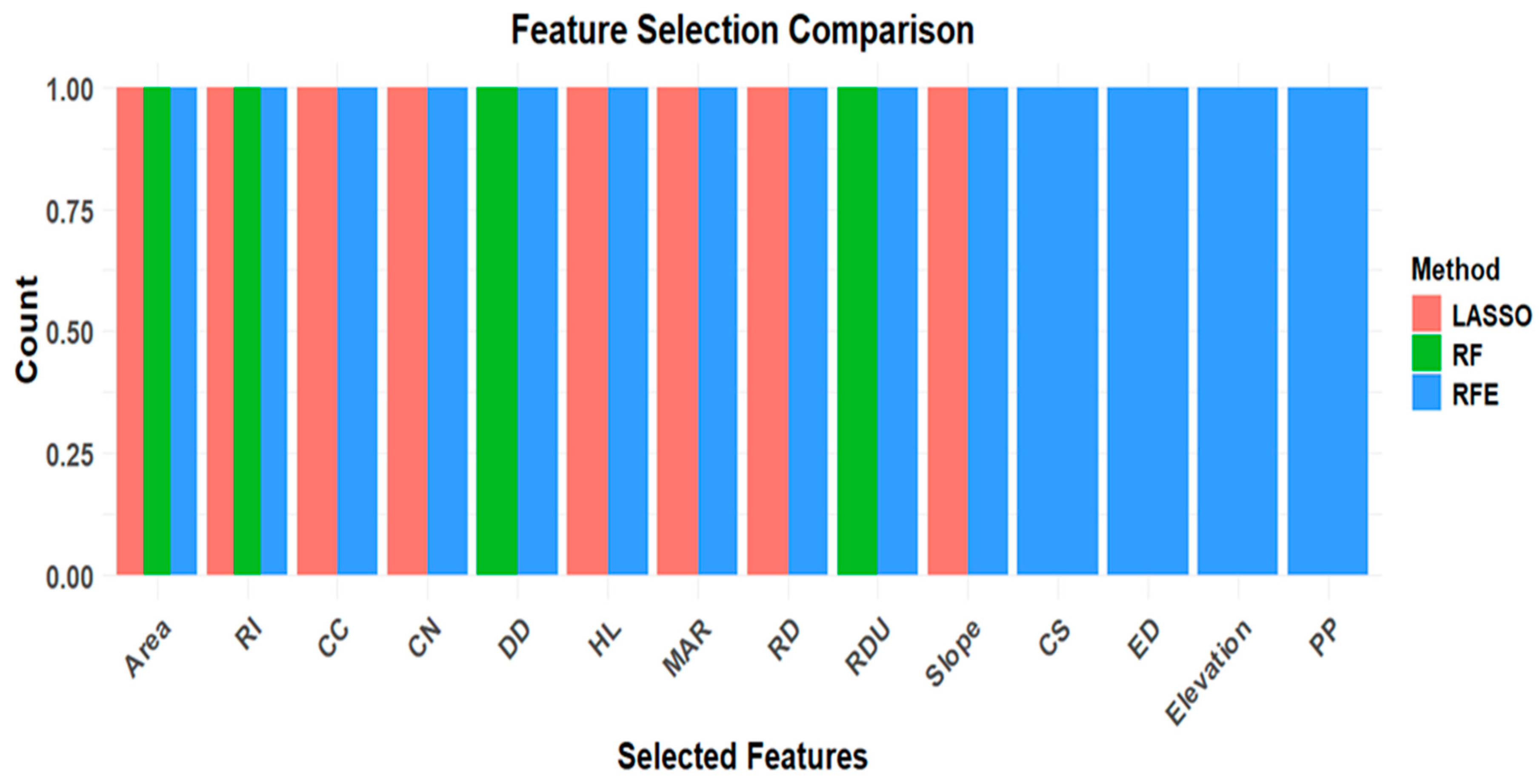
By pinpointing the primary controls on flood lag time, decision-makers can optimize hazard mitigation, ensuring that scarce resources are allocated to the interventions with the greatest impact [50]. To construct a simplified yet robust model, three feature selection techniques—Recursive Feature Elimination (RFE), Least Absolute Shrinkage and Selection Operator (LASSO), and RF importance—were applied (Figure 3). Watershed area (A) and rainfall intensity (RI) consistently emerged as the most important predictors, confirming their dominant role in runoff generation and peak-flow lag time, while curve number (CN) and circularity ratio (CC) appeared as secondary variables in some methods (Figure 5). Although antecedent soil moisture, land cover, soil properties, and drainage characteristics are widely recognized as important controls on runoff generation and flood response, their influence was represented only partially in the present framework. Specifically, weighted Curve Numbers (CNs) were derived following the [10] methodology, which integrates land use, hydrologic soil group, hydrologic condition, and the standard antecedent moisture condition (AMC) based on 5-day antecedent rainfall. Likewise, drainage characteristics were represented by drainage density. However, these variables were not retained in the final empirical model because their additional contribution to predictive performance was smaller than that of watershed area and rainfall intensity. This finding does not imply that these factors are hydrologically unimportant. Our recent global synthesis [57] showed that the dominant controls on lag time vary with climate and watershed scale, with flow-resistance parameters such as CN being particularly important in humid and sub-humid watersheds, whereas channel geometry plays a greater role in drier regions. Under the available dataset, their effects were largely captured through the dominant predictors or indirectly represented by CN. Future studies incorporating direct soil-moisture observations, dynamic antecedent wetness indicators, and larger multi-watershed datasets may further improve prediction accuracy and model transferability.
Figure 5.
Comparison of feature selection methods (Lasso, RF, and RFE) based on the frequency of selected features. The bar heights represent the relative count of features retained by each method, highlighting differences in their selectivity.
The dominance of watershed area (A) and rainfall intensity (RI) is hydrologically consistent with runoff generation in tropical highland watersheds. Watershed area integrates key geomorphological characteristics, including flow-path length, drainage network organization, storage capacity, and travel distance, resulting in longer lag times in larger catchments. In contrast, rainfall intensity provides the primary event-scale forcing that controls the rate of runoff generation and its connectivity to the drainage network. This relationship is consistent with the predominance of saturation-excess runoff in humid tropical environments, where runoff develops as saturated source areas expand and become hydraulically connected [67,68]. Soil depth, land-use condition, vegetation cover, and drainage connectivity further regulate this process by influencing infiltration and subsurface storage. Although these dynamic watershed characteristics were not explicitly included in the empirical model, they provide a physical explanation for the consistent importance of rainfall intensity across watersheds with contrasting geomorphological characteristics.
These feature-selection results also agree with broader hydrological understanding that no single watershed characteristic universally controls flood response timing. Watershed area emerged as the dominant structural predictor because it integrates several correlated geomorphological properties, including hydraulic length, perimeter, and drainage organization, whereas rainfall intensity represents the principal event-scale forcing. Consequently, the feature-selection procedures favored predictors that explained unique variance while minimizing redundancy among highly correlated morphometric variables. Variables such as hydraulic length, drainage density, slope, and circularity ratio were therefore excluded from the final model not because they lack hydrological significance but because much of their explanatory information was already represented by watershed area or contributed comparatively little additional predictive power.
An initial four-variable regression (Equation (1)) achieved reasonable accuracy (R2 = 0.52, RMSE = 5.78), but diagnostics checks confirmed that A (km2) and RI (mm/h) explained most of the variance in TL (h). To enhance interpretability and minimize multicollinearity, the model was simplified to retain only these two dominant predictors.
TL = 12.728 + 0.012 × Area − 0.033 × RI − 1.806 × CC − 0.135 × CN
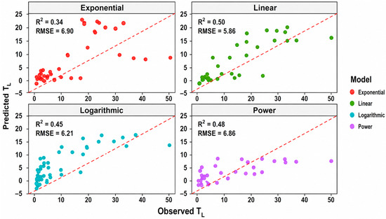
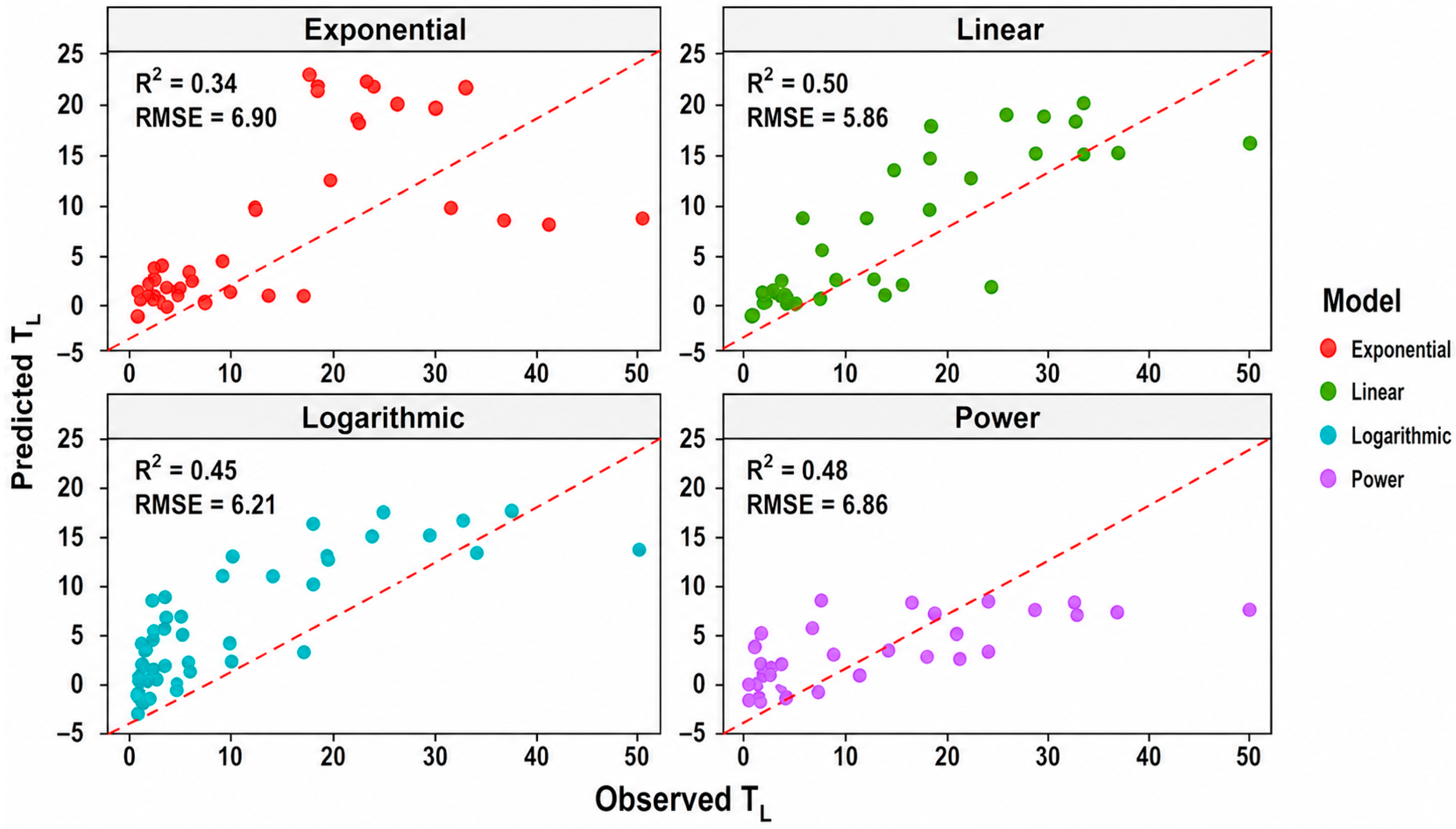
Alternative functional forms were tested (Linear, Power, Exponential, Logarithmic; Figure 6). Among them, the Linear form performed best (Table 2; R2 = 0.51, RMSE = 5.2) and was selected as the final ML-informed empirical model (Equation (2)), where TL is in hours (h), Area is in square kilometers (km2), and rainfall intensity (RI) is in millimeters per hour (mm h−1):
TL = 0.8 + 0.011 × Area − 0.023 × RI
Figure 6.
Observed vs. predicted TL across Linear, Power, Exponential, and Logarithmic regression models (based on two-variable inputs: Area and Rainfall Intensity).
Table 2.
Performance statistics of the 10 conventional empirical equations reported by Sultan et al. [14] for six tropical watersheds, based on watershed-level median observed TL values, compared with the proposed ML-informed model developed in the present study.
Accordingly, the regression coefficients have units of h km−2 (0.011) and h2 mm−1 (0.023), ensuring dimensional consistency of all terms in the equation.
The regression coefficients were statistically significant at p < 0.01, with standard errors of 0.025 for Area and 0.089 for Rainfall Intensity (Table S4). The 95% confidence intervals for the coefficients were [−0.136, −0.038] for Area and [0.138, 0.486] for Rainfall Intensity, confirming the robustness of the estimated relationships. Because multiple events were sampled within the same watershed, observations have a hierarchical structure with repeated watershed-level predictors. Thus, regression p-values and confidence intervals are interpreted as measures of association within the event-level dataset, not evidence from 302 independent watersheds. The empirical relationship is therefore a calibrated association within the observed range, rather than a causal or universally transferable relationship. Residual diagnostics indicated that model assumptions were reasonably satisfied (Shapiro–Wilk normality test: p = 0.342; Breusch–Pagan heteroscedasticity test: p = 0.092; Durbin–Watson autocorrelation test: d = 1.823; Table S5), further supporting the reliability of the regression results.
This simplified two-variable model (Empirical_Var2) explained 51% of TL variance, with the lowest prediction bias (–4.2%), providing a practical balance between predictive performance, simplicity, and operational feasibility (Figure 7). Although its explanatory power is lower than that of the best-performing machine learning models, its transparent structure and minimal data requirements make it particularly suitable for preliminary flood-lag-time estimation in data-scarce tropical watersheds. While ensemble ML models such as RF and XGB achieved higher predictive skill (R2 ≈ 0.65, NSE ≈ 0.60), they required multiple morphometric and climatic inputs. In contrast, Empirical_Var2 relied on only two easily measurable parameters, making it more practical for data-scarce tropical basins.
Figure 7.
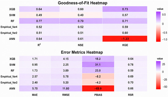
Comparison of machine learning and empirical models (Empirical_Var2 and Empirical_Var4) for predicting flood lag time on the testing dataset, showing goodness-of-fit (R2, KGE, NSE) and error metrics (MAE, RMSE, PBIAS, RSR).
Although the proposed model uses only watershed area and rainfall intensity, previous field observations provide additional insight into the hydrological processes governing event-to-event variability. Ref. [14] demonstrated that lag time varied considerably throughout the rainy season despite relatively small differences in rainfall depth. Watersheds generally exhibited shorter lag times during the early rainy season and progressively longer responses toward the end of the season, reflecting seasonal changes in antecedent soil moisture, vegetation growth, and surface cover conditions. These observations suggest that rainfall intensity is an important event-scale driver, while evolving catchment wetness and storage conditions also influence watershed response but were not explicitly represented in the present empirical model.
Model performance reflects the bias–variance tradeoff: low-complexity models tend to underfit (high bias), while highly flexible models risk overfitting (high variance) [31]. Comparative studies in Ethiopian highland watersheds have demonstrated that while complex ensemble methods like Random Forests achieve high predictive accuracy, simpler models can provide comparable performance with greater interpretability and fewer data requirements [29]. Hybrid approaches, such as the block-based ANN (MB2) [46], demonstrate that leveraging data-rich regions can improve predictions in data-sparse areas, underscoring the value of balancing predictive accuracy with interpretability.
Overall, the ML-informed Empirical_Var2 provides a practical balance between simplicity, accuracy, and interpretability for event-scale flood-lag-time estimation in data-scarce tropical highland watersheds. Requiring only watershed area and rainfall intensity, it has potential for preliminary estimation in ungauged or poorly gauged watersheds, subject to appropriate regional calibration and independent validation.
3.4. Benchmarking Against Existing Empirical Models
Ten widely used empirical lag time equations, originally developed mainly for temperate-region catchments, were evaluated for their transferability to tropical watersheds [14] (Table 2; detailed formulations are provided in Table S2). Overall, most conventional equations exhibited limited predictive capability when applied to the Upper Blue Nile tropical catchments, with several methods showing weak correlations (R2 < 0.25) and considerable systematic biases (e.g., Snyder: −293%, SCS Lag: +163%, and Kirpich: +65%). These results indicate that empirical relationships developed under different climatic, geomorphological, and hydrological conditions may not be directly transferable to tropical environments without local calibration. Among the evaluated approaches, the Simas–Hawkins method showed the highest correlation with observed lag times (R2 = 0.70), indicating its ability to capture important watershed controls. This relatively strong performance is likely related to the inclusion of the curve number (CN), which indirectly represents the combined influence of land cover, soil infiltration characteristics, antecedent moisture conditions, and watershed response characteristics. Similarly, the NRCS Lag approach incorporates CN and watershed characteristics to account for differences in runoff generation mechanisms. Such formulations were developed to represent a broad range of catchment conditions, including smooth agricultural landscapes and forested watersheds with steep channels, where runoff response may be influenced by infiltration processes and subsurface flow contributions [78]. However, despite its relatively high correlation, the Simas–Hawkins method exhibited a considerable prediction bias (PBIAS = −14%) and requires multiple watershed and channel parameters, including characteristics that are often difficult to obtain in poorly monitored tropical regions. Likewise, the SCS Velocity method demonstrated moderate predictive performance (R2 = 0.50; PBIAS = −24%) but depends on additional hydraulic information, which limits its operational application where detailed channel measurements are unavailable.
The regional nature of empirical lag-time relationships has been demonstrated in previous studies. For example, ref. [14] found that the Bransby Williams equation, although developed for tropical India, performed poorly in the Upper Blue Nile Basin. This suggests that climatic similarity alone does not ensure model transferability because watershed response is also controlled by geomorphology, rainfall characteristics, and runoff-generation processes. Similar findings have been reported elsewhere, emphasizing the need for regional calibration of empirical lag-time equations before application beyond their original development area [79].
In comparison, the ML-informed parsimonious model (Empirical_Var2) achieved a moderate but comparable predictive performance (R2 = 0.52; NSE = 0.51) while producing the lowest systematic bias among the tested approaches (PBIAS = −4.2%) using only two readily available predictors: watershed area (A) and rainfall intensity (RI). Although its correlation was lower than that of the [21] equation, the proposed model provides a favorable balance between predictive reliability, bias reduction, simplicity, and applicability for data-limited tropical watersheds. Therefore, the model should be interpreted as a complementary approach rather than a universal replacement for existing empirical formulations.
The advantage of the proposed approach lies in integrating machine-learning-based feature screening with hydrological reasoning to identify a minimal set of physically meaningful predictors. By reducing dependence on detailed geomorphological and hydraulic measurements, the model provides a practical tool for rapid estimation of watershed response time in regions where conventional input datasets are incomplete. This finding is consistent with [41], who demonstrated that large-scale hydrological datasets contain valuable information on catchment behavior that may not be fully represented in existing process-based formulations, and that machine learning can reveal quantitative relationships beyond traditional conceptual understanding.
3.5. Applicability, Limitations and Future Work
The proposed model is applicable to watersheds with areas of 0.58–1655 km2 and rainfall intensities of 0.1–60 mm h−1 (Table 3; Figure S1). Predictions beyond these ranges may be unreliable. Because calibration was based on Ethiopian tropical highland watersheds, its applicability to other hydroclimatic and physiographic settings remains untested.
Table 3.
Ranges and units of the main predictor variables for gauged tropical watersheds.
The machine-learning models were evaluated using a conventional random 80/20 training–testing split after comparison with 70/30 and 75/25 partitions. Although the 80/20 split provided a suitable balance between model calibration and event-level testing, events from the same watershed could occur in both subsets. Therefore, this approach primarily evaluates prediction for new events within watersheds represented in the dataset rather than transferability to entirely unseen watersheds. RF and XGBoost showed the strongest predictive performance, although XGBoost exhibited some overfitting, whereas SVM performed less effectively under heterogeneous event conditions. The empirical model prioritizes interpretability and parsimony over maximum predictive accuracy and should therefore not be used for design-critical applications without further validation. To assess spatial transferability, we additionally conducted watershed-grouped validation using leave-one-watershed-out cross-validation (LOWO-CV) and grouped 5-fold cross-validation, with feature selection and hyperparameter tuning performed independently within each training fold. As shown in Supplementary Table S6, model performance decreased substantially compared with the original event-level evaluation. RF achieved mean R2 values of 0.214 ± 0.338 under LOWO-CV and 0.378 ± 0.247 under grouped 5-fold CV, while XGBoost achieved 0.240 ± 0.306 and 0.334 ± 0.207, respectively. Grouped 5-fold R2 values for SVM and ANN were 0.256 ± 0.293 and 0.202 ± 0.278, respectively. The relatively large variability among held-out watersheds indicates substantial spatial heterogeneity and limited event representation across the 20 watersheds (6–22 events per watershed).
These results highlight an important limitation of the proposed framework: although the models demonstrate useful event-scale predictive capability within the sampled watershed domain, their transferability to unseen or ungauged watersheds remains limited. The relatively small number of events per watershed, spatial heterogeneity, and absence of some potentially important process-relevant variables may constrain generalization. In addition, the performance of increasingly complex machine-learning and deep-learning approaches generally depends on the availability, quality, and temporal resolution of training data, which can be particularly restrictive in data-scarce tropical watersheds. Accordingly, the random-split results should be interpreted primarily as evidence of event-scale predictive capability rather than demonstrated regional or ungauged-watershed transferability. The empirical equation is therefore considered a regionally calibrated formulation for tropical highland watersheds with characteristics comparable to those represented in this study. Application to unseen or ungauged watersheds, particularly beyond the observed predictor ranges, requires additional regional calibration and independent validation. Future research should expand the event database across multiple tropical basins and hydroclimatic settings and evaluate model performance using independent watershed-level and temporal validation. Incorporating process-relevant variables, such as antecedent soil moisture, infiltration characteristics, groundwater conditions, channel roughness, and rainfall spatial variability, may further improve model generalization and hydrological interpretability. Testing advanced deep-learning and hybrid architectures under sufficiently large datasets may also help determine whether their additional complexity provides meaningful improvements over the present parsimonious framework.
Additionally, the TL values used in this study are subject to uncertainties associated with rainfall resolution, centroid estimation, peak-discharge identification, and baseflow separation. Because TL was treated as the observed response variable, formal uncertainty propagation was not performed. Absolute TL values should therefore be interpreted with caution, although the relative relationships identified by the models remain informative.
4. Conclusions
Flood lag time (TL) estimation is critical for flood forecasting and water resource planning in data-limited tropical regions, where climate change and land-use pressures continue to intensify flood risks. This study demonstrates that flood lag time in tropical highland watersheds cannot be explained solely by static geomorphological characteristics; rather, it reflects the combined influence of watershed morphology and rainfall forcing. By applying machine learning (ML) as a diagnostic tool, this study identified watershed area and rainfall intensity as the most important predictors associated with event-scale TL variability. Although dynamic watershed conditions, such as antecedent soil moisture and seasonal vegetation changes, were not explicitly represented, the identified predictors provide a practical basis for developing simplified response-time models. Among the evaluated ML approaches, ensemble methods provided the most robust predictive capability, while the principal contribution of this study was translating ML-derived insights into a parsimonious empirical formulation requiring only two readily available predictors. The proposed two-variable empirical formulation provides a useful balance between predictive performance, interpretability, and simplicity for event-scale flood-lag-time estimation within tropical highland watersheds represented by the study dataset. However, the additional watershed-grouped analysis demonstrated substantially lower predictive performance when entire watersheds were withheld from model development, indicating that the original event-level performance should not be interpreted as evidence of robust transferability to completely unseen or ungauged watersheds. Accordingly, the proposed ML–empirical formulation should be regarded as a regionally calibrated approach for watersheds with hydroclimatic and physiographic characteristics comparable to those represented in this study, rather than as a universally transferable model. Application to other or ungauged watersheds should therefore be preceded by appropriate local or regional calibration and independent watershed-level validation. Overall, the findings demonstrate the potential of ML to enhance hydrological process understanding by revealing the dominant controls embedded within multi-watershed observations and translating these insights into a simple, physically meaningful empirical model. The results also highlight the importance of distinguishing event-level predictive capability from watershed-level spatial generalizability when evaluating ML-based hydrological models. Future studies should use larger multi-basin datasets and fully nested watershed-level validation to assess spatial transferability, incorporate dynamic watershed-state variables such as antecedent soil moisture and rainfall spatial variability, and further develop theory-informed hybrid approaches that integrate data-driven methods with hydrological process understanding.
Supplementary Materials
The following supporting information can be downloaded at: https://www.mdpi.com/article/10.3390/w18172121/s1, Table S1: Summary of hydrological data sources, gauging stations, and watershed characteristics; Table S2: Empirical methods used to estimate lag time and time of concentration in watersheds with different flow regimes and climatic regions worldwide (adapted from Sultan et al., [14]); Table S3: Variance Inflation Factor (VIF) analysis of the predictor variables used in the study; Table S4: Regression coefficients with corresponding 95% confidence intervals for the fitted model; Table S5. Residual diagnostics for the fitted regression model; Table S6: Comparison of event-level and watershed-grouped cross-validation performance for assessing model transferability to unseen watersheds; Figure S1: Distribution of predictor and response variables across all watersheds. Histograms illustrate the frequency distribution of each variable, highlighting data spread and potential skewness; Figure S2: Random Forest model error versus number of trees, showing the variation in prediction error as the number of trees in the ensemble increases.
Author Contributions
Conceptualization, D.S., N.H., M.T., A.A.F., T.A., S.B.K., A.M. and A.T.; methodology, D.S., N.H., M.T., A.A.F., D.A.M., S.B.K., A.M. and A.T.; software, D.S., A.A.F., D.A.M. and S.B.K.; validation, D.S. and A.A.F.; formal analysis, D.S., A.A.F., D.A.M., S.B.K., A.M. and B.A.T.; investigation, D.S., N.H., M.T., A.A.F., T.A., D.A.M., S.B.K. and A.T.; resources, D.S., N.H., A.A.F. and B.A.T.; data curation, D.S., N.H., A.A.F., T.A., A.M. and B.A.T.; writing—original draft preparation, D.S., N.H., M.T., A.A.F., T.A., D.A.M., S.B.K., A.M. and B.A.T.; writing—review and editing, D.S., N.H., M.T., A.A.F., T.A., D.A.M., S.B.K., A.M. and B.A.T.; visualization, D.S., N.H., M.T., A.A.F., D.A.M. and A.T.; supervision, D.S., N.H., M.T., T.A. and A.T.; project administration, N.H.; funding acquisition, N.H. All authors have read and agreed to the published version of the manuscript.
Funding
This research was funded by Japan Society for the Promotion of Science grant number 23KF0258.
Data Availability Statement
The original contributions presented in this study are included in the article/Supplementary Material. Further inquiries can be directed to the corresponding author.
Acknowledgments
D. Sultan gratefully acknowledges the International Platform for Dryland Research and Education (IPDRE), Tottori University, for providing a supportive research environment. This research was supported by the Japan Society for the Promotion of Science (JSPS) Postdoctoral Fellowship.
Conflicts of Interest
The authors declare no conflicts of interest.
References
- Sidle, R.C. Hydrogeomorphic processes in temperate and tropical forests: Effects of land use and scale. Geogr. Compass 2010, 4, 1115–1132. [Google Scholar] [CrossRef] [Scilit]
- Mekonnen, M.A.; Wörman, A.; Dargahi, B.; Gebeyehu, A. Hydrological modelling of Ethiopian catchments using limited data. Hydrol. Process. 2009, 23, 3401–3408. [Google Scholar] [CrossRef] [Scilit]
- Setegn, S.G.; Srinivasan, R.; Melesse, A.M.; Dargahi, B. SWAT model application and prediction uncertainty analysis in the Lake Tana Basin, Ethiopia. Hydrol. Process. 2009, 24, 357–367. [Google Scholar] [CrossRef] [Scilit]
- Steenhuis, T.S.; Collick, A.S.; Easton, Z.M.; Leggesse, E.S.; Bayabil, H.K.; White, E.D.; Ahmed, A.A. Predicting discharge and sediment for the Abay (Blue Nile) with a simple model. Hydrol. Process. Int. J. 2009, 23, 3728–3737. [Google Scholar] [CrossRef] [Scilit]
- Tebebu, T.Y.; Steenhuis, T.S.; Dagnew, D.C.; Guzman, C.D.; Bayabil, H.K.; Zegeye, A.D.; Collick, A.S.; Langan, S.; MacAlister, C.; Langendoen, E.J.; et al. Improving efficacy of landscape interventions in the (sub) humid Ethiopian highlands by improved understanding of runoff processes. Front. Earth Sci. 2015, 3, 49. [Google Scholar] [CrossRef] [Scilit]
- Tilahun, S.A.; Guzman, C.D.; Zegeye, A.D.; Engda, T.A.; Collick, A.S.; Rimmer, A.; Steenhuis, T.S. An efficient semi-distributed hillslope erosion model for the subhumid Ethiopian Highlands. Hydrol. Earth Syst. Sci. 2013, 17, 1051–1063. [Google Scholar] [CrossRef] [Scilit]
- Chang, F.J.; Hsu, K.; Chang, L.C. (Eds.) Flood Forecasting Using Machine Learning Methods; MDPI: Basel, Switzerland, 2019. [Google Scholar]
- Yoo, C.; Lee, J.; Cho, E. Theoretical evaluation of concentration time and storage coefficient with their application to major dam basins in Korea. Water Supply 2019, 19, 644–652. [Google Scholar] [CrossRef] [Scilit]
- Fang, X.; Thompson, D.B.; Cleveland, T.G.; Pradhan, N.R.; Malla, R. Time of Concentration Estimated Using Watershed Parameters Determined by Automated and Manual Methods. J. Irrig. Drain. Eng. 2008, 134, 202–211. [Google Scholar] [CrossRef] [Scilit]
- Gericke, O.J.; Smithers, J.C. Review of methods used to estimate catchment response time for the purpose of peak discharge estimation. Hydrol. Sci. J. 2014, 59, 1935–1971. [Google Scholar] [CrossRef] [Scilit]
- NRCS (Natural Resource Conservation Service). Time of concentration. In National Engineering Handbook: Part 630—Hydrology; USDA Soil Conservation Service: Washington, DC, USA, 2010. [Google Scholar]
- Brutsaert, W. Hydrology: An Introduction; Cambridge University Press: Cambridge, UK, 2005. [Google Scholar]
- McDonnell, J.J.; Beven, K. Debates-The future of hydrological sciences: A (common) path forward? A call to action aimed at understanding velocities, celerities and residence time distributions of the headwater hydrograph. Water Resour. Res. 2014, 50, 5342–5350. [Google Scholar] [CrossRef] [Scilit]
- Sultan, D.; Tsunekawa, A.; Tsubo, M.; Haregeweyn, N.; Adgo, E.; Meshesha, D.T.; Fenta, A.A.; Ebabu, K.; Berihun, M.L.; Setargie, T.A. Evaluation of lag time and time of concentration estimation methods in small tropical watersheds in Ethiopia. J. Hydrol. Reg. Stud. 2022, 40, 101025. [Google Scholar] [CrossRef] [Scilit]
- Sultan, D.; Tsunekawa, A.; Tsubo, M.; Haregeweyn, N.; Adgo, E.; Meshesha, D.T.; Berihun, M.L.; Fenta, A.A.; Ebabu, K.; Setargie, T.A. Analyzing the influence of changes in land use and management practices on the lag time of peak flows for tropical watersheds of Ethiopia. River Res. Appl. 2023, 39, 1148–1159. [Google Scholar] [CrossRef] [Scilit]
- Innocente, C.; Borges Chaffe, P.L.; Speckhann, G.A.; de Almeida Mota, A.; Grison, F.; Kobiyama, M. Time of concentration of small sub-tropical basins. In EGU General Assembly Conference Abstracts; European Geosciences Union: Vienna, Austria, 2018; p. 10992. [Google Scholar]
- Michailidi, E.M.; Antoniadi, S.; Koukouvinos, A.; Bacchi, B.; Efstratiadis, A. Timing the time of concentration: Shedding light on a paradox. Hydrol. Sci. J. 2018, 63, 721–740. [Google Scholar] [CrossRef] [Scilit]
- ERA (Ethiopian Road Authority) Design Manual. 2013. Available online: https://www.scribd.com/document/589878320/ (accessed on 1 October 2025).
- McCuen, R.H. Uncertainty analyses of watershed time parameters. J. Hydrol. Eng. 2009, 14, 490–498. [Google Scholar] [CrossRef] [Scilit]
- McCuen, R.H.; Wong, S.L.; Rawls, W.J. Estimating urban time of concentration. J. Hydraul. Eng. 1984, 110, 887–904. [Google Scholar] [CrossRef] [Scilit]
- Simas, M.J.; Hawkins, R.H. Lag time characteristics for small watersheds in the U.S. In Proceedings of the 2nd Federal Interagency Hydrologic Modeling Conference, (HMC ’02), Las Vegas, NV, USA, July 28–August 1 2002. [Google Scholar]
- Sultan, D.; Tsunekawa, A.; Haregeweyn, N.; Adgo, E.; Tsubo, M.; Meshesha, D.T.; Masunaga, T.; Aklog, D.; Fenta, A.A.; Ebabu, K. Efficiency of soil and water conservation practices in different agro-ecological environments in the Upper Blue Nile Basin of Ethiopia. J. Arid. Land 2018, 10, 249–263. [Google Scholar] [CrossRef] [Scilit]
- Sultan, D.; Tsunekawa, A.; Haregeweyn, N.; Adgo, E.; Tsubo, M.; Meshesha, D.T.; Masunaga, T.; Aklog, D.; Fenta, A.A.; Ebabu, K. Analyzing the runoff response to soil and water conservation measures in a tropical humid Ethiopian highland. Phys. Geogr. 2017, 38, 423–447. [Google Scholar] [CrossRef] [Scilit]
- Dile, Y.T.; Tekleab, S.; Ayana, E.K.; Gebrehiwot, S.G.; Worqlul, A.W.; Bayabil, H.K.; Yimam, Y.T.; Tilahun, S.A.; Daggupati, P.; Karlberg, L.; et al. Advances in water resources research in the Upper Blue Nile basin and the way forward: A review. J. Hydrol. 2018, 560, 407–423. [Google Scholar] [CrossRef] [Scilit]
- Beven, K. A manifesto for the equifinality thesis. J. Hydrol. 2006, 320, 18–36. [Google Scholar] [CrossRef] [Scilit]
- Aljohani, F.H.; Alkhodre, A.B.; Sen, A.A.A.; Ramazan, M.S.; Alzahrani, B.; Siddiqui, M.S. Flood Prediction using Hydrologic and ML-based Modeling: A Systematic Review. Int. J. Adv. Comput. Sci. Appl. 2023, 14. [Google Scholar] [CrossRef] [Scilit]
- Hadia, F.A.A.; Sidek, L.M.; Salih, G.H.A.; Basri, H.; Sammen, S.S.; Dome, N.M.; Ali, Z.M.; Ahmed, A.N. Machine learning techniques for flood forecasting. J. Hydroinform. 2024, 26, 779–799. [Google Scholar] [CrossRef] [Scilit]
- Nevo, S.; Morin, E.; Gerzi Rosenthal, A.; Metzger, A.; Barshai, C.; Weitzner, D.; Voloshin, D.; Kratzert, F.; Elidan, G.; Dror, G.; et al. Flood forecasting with machine learning models in an operational framework. Hydrol. Earth Syst. Sci. 2022, 26, 4013–4032. [Google Scholar] [CrossRef] [Scilit]
- Shortridge, J.E.; Guikema, S.D.; Zaitchik, B.F. Machine learning methods for empirical streamflow simulation: A comparison of model accuracy, interpretability, and uncertainty in seasonal watersheds. Hydrol. Earth Syst. Sci. 2016, 20, 2611–2628. [Google Scholar] [CrossRef] [Scilit]
- Vizi, Z.; Batki, B.; Rátki, L.; Szalánczi, S.; Fehérváry, I.; Kozák, P.; Kiss, T. Water level prediction using long short-term memory neural network model for a lowland river: A case study on the Tisza River, Central Europe. Environ. Sci. Eur. 2023, 35, 92. [Google Scholar] [CrossRef] [Scilit]
- Lucie-Smith, L. Insights into Cosmological Structure Formation with Machine Learning. Ph.D. Dissertation, UCL (University College London), London, UK, 2020. [Google Scholar]
- See, L.; Solomatine, D.; Abrahart, R.; Toth, E. Hydroinformatics: Computational intelligence and technological developments in water science applications—Editorial. Hydrol. Sci. J. 2007, 52, 391–396. [Google Scholar] [CrossRef] [Scilit]
- Zhou, J.; Chen, L.; Hu, T.; Lu, H.; Shi, Y.; Chen, L. The comparative study of machine learning agent models in flood forecasting for tidal river reaches. Sci. Rep. 2025, 15, 19130. [Google Scholar] [CrossRef] [Scilit] [PubMed]
- Cao, Q.; Zhang, H.; Zhu, F.; Hao, Z.; Yuan, F. Multi-step-ahead flood forecasting using an improved BiLSTM-S2S model. J. Flood Risk Manag. 2022, 15, e12827. [Google Scholar] [CrossRef] [Scilit]
- Yang, S.; Tan, M.L.; Song, Q.; He, J.; Yao, N.; Li, X.; Yang, X. Coupling SWAT and Bi-LSTM for improving daily-scale hydro-climatic simulation and climate change impact assessment in a tropical river basin. J. Environ. Manag. 2023, 330, 117244. [Google Scholar] [CrossRef] [Scilit] [PubMed]
- Farfán-Durán, J.F.; Cea, L. Streamflow forecasting with deep learning models: A side-by-side comparison in Northwest Spain. Earth Sci. Inform. 2024, 17, 5289–5315. [Google Scholar] [CrossRef] [Scilit]
- Ghobadi, F.; Kang, D. Improving long-term streamflow prediction in a poorly gauged basin using geo-spatiotemporal mesoscale data and attention-based deep learning: A comparative study. J. Hydrol. 2022, 615, 128608. [Google Scholar] [CrossRef] [Scilit]
- Khatun, A.; Nisha, M.N.; Chatterjee, S.; Sridhar, V. A novel insight on input variable and time lag selection in daily streamflow forecasting using deep learning models. Environ. Model. Softw. 2024, 179, 106126. [Google Scholar] [CrossRef] [Scilit]
- Tripathy, K.P.; Mishra, A.K. Deep learning in hydrology and water resources disciplines: Concepts, methods, applications, and research directions. J. Hydrol. 2024, 628, 130458. [Google Scholar] [CrossRef] [Scilit]
- Hasan, M.H.; Ahmed, A.; Nafee, K.M.; Hossen, M.A. Use of machine learning algorithms to assess flood susceptibility in the coastal area of Bangladesh. Ocean Coast. Manag. 2023, 236, 106503. [Google Scholar] [CrossRef] [Scilit]
- Nearing, G.S.; Kratzert, F.; Sampson, A.K.; Pelissier, C.S.; Klotz, D.; Frame, J.M.; Prieto, C.; Gupta, H.V. What role does hydrological science play in the age of machine learning? Water Resour. Res. 2021, 57, e2020WR028091. [Google Scholar] [CrossRef] [Scilit]
- Pion-Tonachini, L.; Bouchard, K.; Martin, H.G.; Peisert, S.; HoTLz, W.B.; Aswani, A.; Dwivedi, D.; Wainwright, H.; Pilania, G.; Nachman, B.; et al. Learning from learning machines: A new generation of AI technology to meet the needs of science. arXiv 2021, arXiv:2111.13786. [Google Scholar]
- Ankah, M.L.Y.; Adjei-Yeboah, S.; Ziggah, Y.Y.; Asare, E.N. Advanced hybrid machine learning models with explainable AI for predicting residual friction angle in clay soils. Sci. Rep. 2025, 15, 25868. [Google Scholar] [CrossRef] [Scilit] [PubMed]
- Naeini, S.S.; Snaiki, R. A novel hybrid machine learning model for rapid assessment of wave and storm surge responses over an extended coastal region. Coast. Eng. 2024, 190, 104503. [Google Scholar] [CrossRef] [Scilit]
- Rudin, C.; Chen, C.; Chen, Z.; Huang, H.; Semenova, L.; Zhong, C. Interpretable machine learning: Fundamental principles and 10 grand challenges. Stat. Surv. 2022, 16, 1–85. [Google Scholar] [CrossRef] [Scilit]
- Xie, S.; Wu, W.; Mooser, S.; Wang, Q.J.; Nathan, R.; Huang, Y. Artificial neural network based hybrid modeling approach for flood inundation modeling. J. Hydrol. 2021, 592, 125605. [Google Scholar] [CrossRef] [Scilit]
- Wielinga, S.; Heyninck, J. Interpretable Hybrid Machine Learning Models Using FOLD-R++ and Answer Set Programming. arXiv 2025, arXiv:2506.19573. [Google Scholar]
- Worku, K.B.; Bronstert, A.; Francke, T.; Zimale, F.A. Combining Machine Learning and Process-Based Modelling for Sediment Load Estimation in the Data-Scarce Upper Blue Nile Basin. Water 2026, 18, 1759. [Google Scholar] [CrossRef] [Scilit]
- Parvandeh, S.; Yeh, H.W.; Paulus, M.P.; McKinney, B.A. Consensus features nested cross-validation. Bioinformatics 2020, 36, 3093–3098. [Google Scholar] [CrossRef] [Scilit] [PubMed]
- Leggesse, E.S.; Derseh, W.A.; Zimale, F.A.; Tilahun, S.A.; Meshesha, M.A. Urban flash flood hazard mapping using machine learning, Bahir Dar, Ethiopia. J. Hydroinform. 2024, 26, 2124–2145. [Google Scholar] [CrossRef] [Scilit]
- Setargie, T.A.; Tsunekawa, A.; Haregeweyn, N.; Tsubo, M.; Fenta, A.A.; Berihun, M.L.; SuTLan, D.; YibeTLal, M.; Ebabu, K.; Nzioki, B.; et al. Random Forest–based gully erosion susceptibility assessment across different agro-ecologies of the Upper Blue Nile basin, Ethiopia. Geomorphology 2023, 431, 108671. [Google Scholar] [CrossRef] [Scilit]
- Dingman, S.L. Physical Hydrology, 2nd ed.; Macmillan: New York, NY, USA, 2002. [Google Scholar]
- Lim, K.J.; Engel, B.A.; Tang, Z.; Choi, J.; Kim, K.S.; Muthukrishnan, S.; Tripathy, D. Automated web GIS based hydrograph analysis tool, WHAT 1. JAWRA J. Am. Water Resour. Assoc. 2005, 41, 1407–1416. [Google Scholar] [CrossRef] [Scilit]
- Giani, G.; Tarasova, L.; Woods, R.A.; Rico-Ramirez, M.A. An objective time-series-analysis method for rainfall-runoff event identification. Water Resour. Res. 2022, 58, e2021WR031283. [Google Scholar] [CrossRef] [Scilit]
- Zheng, Y.; Coxon, G.; Woods, R.; Li, J.; Feng, P. Controls on the spatial and temporal patterns of rainfall-runoff event characteristics—A large sample of catchments across Great Britain. Water Resour. Res. 2023, 59, e2022WR033226. [Google Scholar] [CrossRef] [Scilit]
- Wasko, C.; Guo, D. Understanding event runoff coefficient variability across Australia using the hydroEvents R package. Hydrol. Processes 2022, 36, e14563. [Google Scholar] [CrossRef] [Scilit]
- Sultan, D.; Tsunekawa, A.; Haregeweyn, N.; Tsubo, M.; Fenta, A.A.; Ravazzani, G.; Cislaghi, A.; Ebabu, K.; Alem, D.M. Global review of hydrological response time: Analysis and synthesis across diverse climates. Hydrol. Sci. J. 2026. just accepted. [Google Scholar] [CrossRef] [Scilit]
- Leggesse, E.S.; Zimale, F.A.; SuTLan, D.; Enku, T.; Srinivasan, R.; Tilahun, S.A. Predicting optical water quality indicators from remote sensing using machine learning algorithms in tropical highlands of Ethiopia. Hydrology 2023, 10, 110. [Google Scholar] [CrossRef] [Scilit]
- Goel, N. Optimized Prognostic Models for Oral Cancer Survival using Feature Selection Methods. Procedia Comput. Sci. 2024, 235, 1832–1840. [Google Scholar] [CrossRef] [Scilit]
- Guyon, I.; Weston, J.; Barnhill, S.; Vapnik, V. Gene selection for cancer classification using support vector machines. Mach. Learn. 2002, 46, 389–422. [Google Scholar] [CrossRef] [Scilit]
- Scikit-Learn Documentation. Recursive Feature Elimination. Available online: https://scikit-learn.org/stable/modules/feature_selection.html (accessed on 14 August 2025).
- Tibshirani, R. Regression shrinkage and selection via the lasso. J. R. Stat. Soc. Ser. B 1996, 58, 267–288. [Google Scholar] [CrossRef] [Scilit]
- Breiman, L. Random forests. Mach. Learn. 2001, 45, 5–32. [Google Scholar] [CrossRef] [Scilit]
- Zhong, J.; Elsheikha, H.M.; Chan, K.L.A. Optimizing super-feature selection for machine learning-enhanced spectroscopic analysis in biomedical research. Spectrochim. Acta Part A Mol. Biomol. Spectrosc. 2025, 344, 126639. [Google Scholar] [CrossRef] [Scilit] [PubMed]
- Seyam, M.; Othman, F.; El-Shafie, A.; Yaseen, Z.M. Analysis of rainfall intensity impact on the lag time estimation in tropical humid rivers. Int. J. Adv. Appl. Sci. 2017, 4, 15–19. [Google Scholar] [CrossRef] [Scilit]
- Ross, C.A.; Ali, G.A.; Spence, C.; Oswald, C.J.; Phillips, A.K. Reconceptualizing threshold-mediated runoff responses: A case study from the Humber River watershed, Ontario, Canada. Hydrol. Processes 2024, 38, e15241. [Google Scholar] [CrossRef] [Scilit]
- Blöschl, G.; Sivapalan, M. Scale issues in hydrological modelling: A review. Hydrol. Processes 1995, 9, 251–290. [Google Scholar] [CrossRef] [Scilit]
- Pearce, A.J.; Stewart, M.K.; Sklash, M.G. Storm runoff generation in humid headwater catchments: 1. Where does the water come from? Water Resour. Res. 1986, 22, 1263–1272. [Google Scholar] [CrossRef] [Scilit]
- USBR (United States Bureau of Reclamation). Design of Small Dams, 2nd ed.; Water Resources Technical Publications: Washington, DC, USA, 1973. [Google Scholar]
- Snyder, F.F. Synthetic unit-graphs. Eos Trans. Am. Geophys. Union 1938, 19, 447–454. [Google Scholar] [CrossRef] [Scilit]
- SCS (Soil Conservation Service). ‘Hydrology’ National Engineering Handbook. Supplement A, Section 4; U.S. Department of Agriculture: Washington, DC, USA, 1972. [Google Scholar]
- Li, M.H.; Chibber, P. Overland flow time of concentration on very flat terrains. Transp. Res. Rec. 2008, 2060, 133–140. [Google Scholar] [CrossRef] [Scilit]
- FAA (Federal Aviation Administration). Circular on Airport Drainage; Report A/C 050-5320-5B; US. Department of Transportation: Washington DC, USA, 1970. [Google Scholar]
- Kirpich, Z.P. Time of concentration of small agricultural watersheds. Civ. Eng. 1940, 10, 362. [Google Scholar]
- Carter, R.W. Magnitude and frequency of floods in suburban areas. US Geol. Surv. Prof. Pap. 1961, 424, 9–11. [Google Scholar]
- De Almeida, I.K.; Almeida, A.K.; Anache, J.A.; Steffen, J.L.; Sobrinho, T.A. Estimation on time of concentration of overland flow in watersheds: A review. Geosci. Geociências 2014, 33, 661–671. [Google Scholar]
- Kaufmann de Almeida, I.; Kaufmann Almeida, A.; Garcia Gabas, S.; Alves Sobrinho, T. Performance of methods for estimating the time of concentration in a watershed of a tropical region. Hydrol. Sci. J. 2017, 62, 2406–2414. [Google Scholar] [CrossRef] [Scilit]
- Folmar, N.D.; Miller, A.C. Development of an empirical lag time equation. J. Irrig. Drain. Eng. 2008, 134, 501–506. [Google Scholar] [CrossRef] [Scilit]
- Salimi, E.T.; Nohegar, A.; Malekian, A.; Hoseini, M.; Holisaz, A. Estimating time of concentration in large watersheds. Paddy Water Environ. 2017, 15, 123–132. [Google Scholar] [CrossRef] [Scilit]

Disclaimer/Publisher’s Note: The statements, opinions and data contained in all publications are solely those of the individual author(s) and contributor(s) and not of MDPI and/or the editor(s). MDPI and/or the editor(s) disclaim responsibility for any injury to people or property resulting from any ideas, methods, instructions or products referred to in the content. |
© 2026 by the authors. Licensee MDPI, Basel, Switzerland. This article is an open access article distributed under the terms and conditions of the Creative Commons Attribution (CC BY) license.