Gradient-Based Equation Adaptive Weighting in Physics-Informed Neural Networks for Water Hammer Analysis

Abstract

To address the issues of optimization instability and imbalance in the contributions of multiple governing equations in conventional Physics-Informed Neural Networks (PINNs) for hydraulic transient problems, a gradient-based equation adaptive weighting strategy is proposed in this study. This strategy is incorporated into the PINN framework, referred to as GEAW-PINNs (gradient-based equation adaptive weighting in Physics-Informed Neural Networks), for predicting pressure and flow velocity during water hammer events. In GEAW-PINNs, the loss terms associated with different governing equations in the partial differential equation (PDE) constraints are dynamically weighted, thereby enhancing training stability. In the model construction, the classical governing equations of water hammer are employed to establish the PDE constraints, in which the Brunone model is incorporated. Meanwhile, the corresponding model coefficient is treated as a trainable parameter, enabling simultaneous parameter inversion and prediction of pressure and flow velocity. High-accuracy numerical solutions are generated as reference data to validate the proposed framework. The results demonstrate that GEAW-PINN effectively improves the stability of PINNs for the prediction of pressure in water hammer phenomena, thereby enhancing overall optimization performance and prediction accuracy. For the reservoir–pipeline–valve system, the proposed method achieved relative errors of only 0.00742 for pressure and 0.0183 for velocity. And the proposed method can also provide accurate predictions in complex pipe network systems. For the pipeline network system, the absolute prediction errors were approximately 15 for pressure and 0.05 for velocity. Finally, the robustness of the proposed method was evaluated under different random seeds and 25 dB noise. The prediction error exhibited little variation across different random seeds, with a variance of only $1.1429\times {10}^{-7}$ and $6.87\times {10}^{-7}$. Under 25 dB noise, the prediction error increased only slightly to $9.88\times {10}^{-3}$ and $2.5\times {10}^{-2}$. This study provides a practical example for achieving stable PINN training in multi-physics coupled problems.

1. Introduction

In water supply networks, hydropower systems, and long-distance water transmission projects, fluids are typically conveyed through pipelines. During system start-up and shutdown, valve operations, or variations in operating conditions, rapid acceleration or deceleration of the fluid may occur, leading to significant transient flow phenomena, commonly referred to as water hammer. The resulting pressure fluctuations can reach high amplitudes within a short period, posing potential threats to the safety of pipelines and valves [1,2]. Therefore, accurate prediction of transient pressure and flow velocity in pipeline systems is of great importance for ensuring the safe and stable operation of hydraulic systems.

For transient flow problems in pipelines, traditional approaches mainly include the Method of Characteristics (MOC) [3], Finite Difference Method (FDM) [4], and Finite Volume Method (FVM) [5]. These methods obtain approximate solutions to the governing partial differential equations of transient flow, thereby enabling the calculation of pressure and flow velocity. However, their application typically relies on complete and accurate initial conditions, boundary conditions, and system parameters. In practical engineering scenarios, due to varying operating conditions and parameter uncertainties—such as pipe roughness, wave speed, and unsteady friction effects—these requirements are often difficult to satisfy, which limits the applicability of traditional methods.

With the development of monitoring technologies, pressure and flow sensors have been increasingly deployed in pipeline systems, providing support for data-driven approaches. Physics-Informed Neural Networks (PINNs) were first proposed by Raissi et al. [6]. Unlike purely data-driven models, PINNs are capable of leveraging the underlying physical laws embedded in observational data to solve nonlinear partial differential equations and infer unknown parameters [7,8]. Owing to their high accuracy in modeling complex dynamics under incomplete models and sparse data conditions [9], PINNs have been widely applied in various fields, including mechanical engineering [10], density functional theory (DFT) calculations in chemistry [11], new material development [12], and computational fluid dynamics (CFD) [13,14]. Researchers have improved the accuracy, stability and convergence speed of PINNs by modifying network architectures [14,15], activation functions [16,17], loss functions [18], and training strategies [19,20]. For transient pipe flow problems, Ye et al. [21] employed a PINN incorporating a steady friction term in the water hammer equations to predict one-dimensional pipe flow, while Xu et al. [22] introduced adaptive activation functions and a water hammer model with an unsteady friction term to enhance prediction performance for one-dimensional pipeline flow. The water hammer phenomenon is governed by a system of two physical equations. Due to the significant scale disparity between these governing equations, PINNs often suffer from training instability and convergence difficulties, which in turn degrade prediction accuracy. In recent years, extensive research has been conducted on multi-physics PINNs [23,24], with approaches primarily focusing on modifying sampling strategies [25] and loss functions [26]. Most of these methods aim to alleviate the imbalance by adaptively adjusting loss weights based on gradient information [27].

To address these challenges, a gradient-based equation adaptive weighting strategy is proposed and incorporated into a PINN framework for transient flow prediction in pipelines, referred to as GEAW-PINNs. In this framework, adaptive weights are assigned to different governing equations, enabling dynamic adjustment of their contributions during training and alleviating the imbalance among multi-physics equations. Meanwhile, an instantaneous acceleration-based unsteady friction model is introduced to enhance the physical constraints, and the corresponding coefficient in the Brunone model is treated as a trainable parameter to improve the model’s adaptability to parameter uncertainties [28].

To validate the effectiveness of GEAW-PINNs, high-accuracy reference solutions are generated using a weighted unsteady friction model [29,30,31] combined with the MOC, and comprehensive evaluations are conducted. And GEAW-PINNs extend to complex pipe network systems. The model was further evaluated under different random seeds and 25 dB noise. The results demonstrate that GEAW-PINNs can accurately predict transient pressure and flow velocity under sparse observation conditions, improving training stability and prediction accuracy compared with the PINN framework employing adaptive activation functions in the water hammer study by Xu et al. [22], while enabling parameter inversion. This study provides a useful reference for water hammer prediction and offers insights into stabilizing PINN training in multi-physics coupled problems.

2. Methodology

2.1. Governing Equations of Classical Water Hammer

To describe transient flow in pipeline systems, a one-dimensional hydraulic transient process is considered, in which the fluid motion is assumed to be primarily along the axial direction of the pipe, while radial velocity components and cross-sectional non-uniformities are neglected. The transient flow in pressurized pipelines is governed by a set of continuity and momentum equations [3]:

$${\displaystyle \frac{\partial H}{\partial t}}+{\displaystyle \frac{a^2}{g}}{\displaystyle \frac{\partial V}{\partial x}}=0$$

(1)

$${\displaystyle \frac{\partial H}{\partial x}}+{\displaystyle \frac{1}{g}}{\displaystyle \frac{\partial V}{\partial t}}+J_s=0$$

(2)

where H is the piezometric head, $\mathrm{m}$; t is time, $\mathrm{s}$; a is the wave speed, $\mathrm{m}/\mathrm{s}$; g is the gravitational acceleration, $\mathrm{m}/{\mathrm{s}}^2$; V is the flow velocity, $\mathrm{m}/\mathrm{s}$; x is the distance along the pipeline, $\mathrm{m}$; and f is the Darcy–Weisbach friction factor. And J is the term representing the friction force per unit weight. It is typically expressed as $J_s=fV\left|V\right|/2gD$, where D is the pipe diameter, $\mathrm{m}$.

Previous studies on water hammer have proposed several unsteady friction models, including the weighted unsteady friction model and the instantaneous acceleration-based friction model. Owing to its simple formulation, the instantaneous acceleration-based model incorporates only the local instantaneous acceleration at the current time step, resulting in significantly lower computational cost. Therefore, this model is adopted as the governing friction formulation in the PINN framework to improve computational efficiency.

$$J=J_s+J_u$$

(3)

where $J_u$ denotes the unsteady friction term. The instantaneous acceleration-based friction model incorporates the local instantaneous acceleration at the current time step into the friction formulation. Owing to its simple formulation and low computational cost, this model is adopted as the physical constraint in the proposed PINN framework to improve computational efficiency [22].

$$J_u=k\left({\displaystyle \frac{\partial V}{\partial t}}-a{\displaystyle \frac{\partial V}{\partial x}}\right)$$

(4)

where k is the Brunone coefficient.

The weighted unsteady friction model accounts for flow history through the convolution of the weighting function with the past velocity variations, thereby providing a more accurate description of unsteady friction. To reduce the associated computational cost, the weighting function is commonly approximated by a series of exponential terms. The coefficients adopted in this study are listed in Table 1 [31]. Owing to its high accuracy, the weighted unsteady friction model is employed to generate the reference solutions.

$$\begin{array}{cc}\hfill J_u& ={\displaystyle \frac{16\mu }{g{D}^2}}{\int }_0^t{\displaystyle \frac{\partial V}{\partial t}}\left(t^{\prime }\right)\mathcal{W}(t-t^{\prime })d{t}^{\prime },\hfill \end{array}$$

(5)

$$\begin{array}{cc}\hfill \mathcal{W}\left(\tau \right)& ={\displaystyle \sum _{i=1}^N}{m}_i{e}^{-n_i\tau }.\hfill \end{array}$$

(6)

where $\mu$ is the kinematic viscosity coefficient, and $\mathcal{W}\left(\tau \right)$ is a weighted function.

Table 1. Coefficients $m_i$ and $n_i$.

i	1	2	3	4	5	6	7	8	9
$m_i$	9.06	$-4.05$	12	8.05	22.7	35.2	65.9	115	206
$n_i$	10	${10}^{1.5}$	${10}^2$	${10}^{2.5}$	${10}^3$	${10}^{3.5}$	${10}^4$	${10}^{4.5}$	${10}^5$
i	10	11	12	13	14	15	16	17
$m_i$	365	651	1150	2060	3630	6640	10,700	26,200
$n_i$	${10}^{5.5}$	${10}^6$	${10}^{6.5}$	${10}^7$	${10}^{7.5}$	${10}^8$	${10}^{8.5}$	${10}^9$

For viscoelastic pipes, the creep function of the pipe wall can be characterized using the mechanical model of a generalized viscoelastic solid [32]:

$$J\left(t\right)=J_0+{\displaystyle \sum _{k=1}^N}{J}_k\left(1-e^{-{\displaystyle \frac{t}{{\tau }_k}}}\right)$$

(7)

where $J_0$ is instantaneous creep compliance; $J_k$ is spring creep compliance in the kth element; and ${\tau }_k$ is the relaxation time of damping in the kth element.

Subsequently, Evangelista et al. [33] conducted valve closure experiments in a three-pipe network and demonstrated that the viscoelastic parameters are intrinsic material properties, independent of the geometric configuration of the pipeline system. Due to the high computational complexity of the viscoelastic model, the instantaneous acceleration-based friction model was adopted as the governing friction formulation in the PINN framework.

2.2. Analysis of PINN for Solving Water Hammer Equations

As an effective physics-driven approach, the Physics-Informed Neural Network (PINN) is employed to model water hammer problems. In this study, the spatial coordinate x and time t are taken as inputs, while the piezometric head $h(x,t)$ and flow velocity $v(x,t)$ are treated as outputs of the network [21].

Under complex operating conditions, the available observational data are usually limited. Assuming that sensors are deployed at several discrete spatial locations, the corresponding time-series measurements of piezometric head or flow velocity can be obtained. The observation dataset can be expressed as:

$$I=\left\{(x_i,t_i,{\varphi }_{ij})\right\}$$

(8)

where ${\varphi }_{ij}$ denotes the observed value at location $x_i$ and time $t_i$, which can represent either the piezometric head or the flow velocity.

Due to the significant differences in physical dimensions and numerical scales among pipeline length, time, piezometric head, and flow velocity (with the piezometric head typically having a larger magnitude), directly training the neural network may lead to imbalance in the loss function, thereby affecting convergence performance and prediction accuracy. Moreover, the governing equations of transient flow usually consist of multiple coupled physical equations. The numerical discrepancies and coupling effects among these equations can further exacerbate optimization difficulties and reduce the accuracy of parameter inversion.

2.3. Construction of Physics-Informed Neural Network

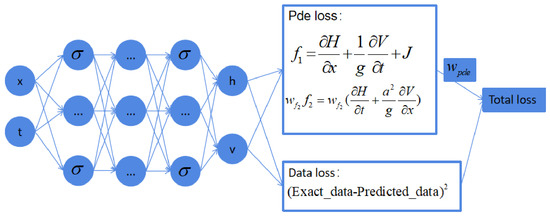
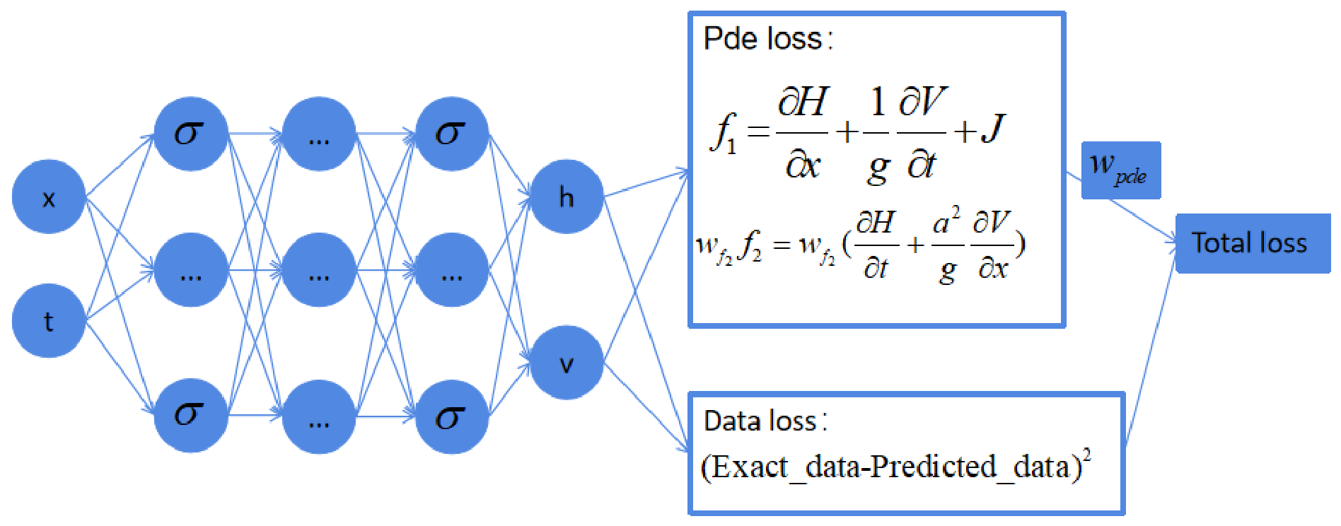
To address the training imbalance caused by scale disparities and multi-physics coupling, the input and output variables are normalized to eliminate differences in magnitude. Furthermore, an adaptive weighting mechanism is introduced for the governing equations, allowing dynamic adjustment of their contributions during training. This improves the imbalance in the optimization process and enhances both training stability and prediction accuracy. The network and modified loss function are shown in Figure 1. The total loss function consists of a data loss term and a physics-based loss term:

$$\begin{array}{cc}\hfill L\left(\theta \right)& =L_{data}+w_{pde}{L}_{pde}\hfill \\ \hfill L_{data}& ={\displaystyle \frac{1}{N_d}}{\displaystyle \sum _{i=1}^{N_d}}{\left(U_i-u(x_d^i,t_d^i;\theta )\right)}^2\hfill \\ \hfill L_{pde}& ={\displaystyle \frac{1}{N_f}}{\displaystyle \sum _{i=1}^{N_f}}\left({\left(f_1(x_f^i,t_f^i;\theta )\right)}^2+{\left(w_{f_2}{f}_2(x_f^i,t_f^i;\theta )\right)}^2\right)\hfill \end{array}$$

(9)

where $\theta$ denotes the trainable parameters of the neural network, and $w_{pde}$ represents the weighting coefficient for the residual loss. $U_i$ is the ground-truth value at the data point, ${\left\{x_f^i,t_f^i\right\}}_{i=1}^{N_f}$ denotes the number of collocation points used to enforce the PDE residuals, and ${\left\{x_d^i,t_d^i\right\}}_{i=1}^{N_d}$ represents the number of training data points. If a measurement location contains m time steps, then $N_f=m_f\times n_f$, where $N_d=m_d\times n_d$ is the number of sensor locations. The weighting coefficient $w_f$ is introduced to balance the scale differences among different governing equations.

Figure 1. The GEAW-PINN structure for transient pipe flow.

To more accurately describe the unsteady friction effects in water hammer processes, the Brunone model is incorporated into the momentum equation. By introducing a local acceleration term, this model better captures the energy dissipation characteristics in transient flows, while maintaining a relatively simple formulation. In addition, following Xu et al.’s approach [22], the Brunone parameter is set as a trainable parameter to improve stability. Therefore, the Brunone model is adopted as part of the governing equation constraints, and $f_1,f_2$ can be expressed as follows:

$$\begin{array}{cc}\hfill f_1& ={\displaystyle \frac{\partial H}{\partial t}}+{\displaystyle \frac{a^2}{g}}{\displaystyle \frac{\partial V}{\partial x}}\hfill \end{array}$$

(10)

$$\begin{array}{cc}\hfill f_2& =g{\displaystyle \frac{\partial H}{\partial x}}+{\displaystyle \frac{\partial V}{\partial t}}+{\displaystyle \frac{f}{2D}}v\left|v\right|+\lambda \left({\displaystyle \frac{\partial V}{\partial t}}-a{\displaystyle \frac{\partial V}{\partial x}}\right)\hfill \end{array}$$

(11)

where the partial derivatives involving H and V are computed via automatic differentiation. The coefficient $\lambda$ is treated as a trainable parameter with an initial value of zero. During training, the optimization process first employs the Adam optimizer [34] with a learning rate of $1\times {10}^{-4}$, followed by a secondary optimization using the L-BFGS algorithm. The coefficient $\lambda$ is kept constant during the L-BFGS stage [35].

After training, the performance of the PINN is evaluated using testing points. The primary evaluation metric is the $L^2$ error [36], defined as follows:

$$L^2={\displaystyle \frac{{∥u(x_e,t_e;\theta )-U_e∥}_2}{{∥U_e∥}_2}}$$

(12)

where $(x_i,t_i)$ denotes the testing point, $u(x_i,t_i;\theta )$ represents the predicted value of the neural network, and $u_e$ is the corresponding reference value. All experiments are conducted on a local workstation equipped with an RTX 4090 GPU.

2.4. Gradient Imbalance Among Governing Equations

In the PINN-based modeling of hydraulic transients, the physical loss terms corresponding to the two governing equations of water hammer can be denoted as $L_1$ and $L_2$. During backpropagation, the gradients of the loss function with respect to the network parameters $\theta$ can be expressed as

$$\begin{array}{cc}\hfill {\nabla }_{\theta }{L}_{pde}& ={\nabla }_{\theta }{L}_{f_1}+{\nabla }_{\theta }{L}_{f_2}\hfill \end{array}$$

(13)

$$\begin{array}{cc}\hfill L_{f_1}& ={\displaystyle \frac{1}{N_f}}\sum f_1^2,L_{f_2}={\displaystyle \frac{1}{N_f}}\sum f_2^2\hfill \end{array}$$

(14)

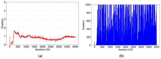
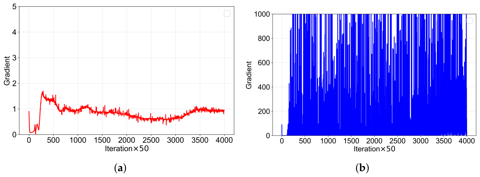
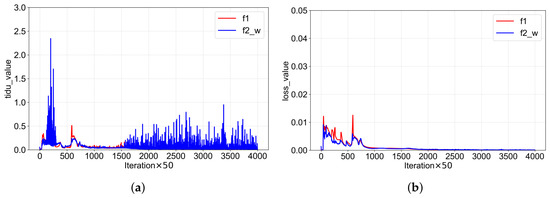
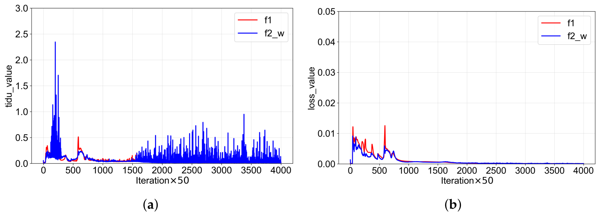
When $∥{\nabla }_{\theta }{L}_{f_2}∥\gg ∥{\nabla }_{\theta }{L}_{f_1}∥$, the optimization process is dominated by $f_2$, making it difficult for the physical constraint associated with $f_1$ to be effectively learned. The comparison of their gradient magnitudes is illustrated in Figure 2, where the gradient of $f_2$ is significantly larger than that of $f_1$ and exhibits more frequent oscillations. This gradient imbalance reduces the model’s ability to learn multiple physical equations in a coordinated manner, thereby degrading overall prediction accuracy and convergence stability.

Figure 2. Comparison of gradients of $f_1$ and $f_2$ during training: (a) $f_1$, (b) $f_2$.

To balance the gradient contributions of the two governing equations, the weighting coefficients are defined as follows:

$$\begin{array}{cc}\hfill L_{pde}& =L_{f_1}+\left(w_{f_2}^2{L}_{f_2}\right)\hfill \end{array}$$

(15)

$$\begin{array}{cc}\hfill {\nabla }_{\theta }{L}_{pde}& ={\nabla }_{\theta }{L}_{f_1}+{\nabla }_{\theta }\left(w_{f_2}^2{L}_{f_2}\right)={\nabla }_{\theta }{L}_{f_1}+w_{f_2}^2{\nabla }_{\theta }{L}_{f_2}\hfill \end{array}$$

(16)

To balance the gradient contributions from the two governing equations, the weight assigned to $w_{f_2}$ was calculated as follows:

$$∥{\nabla }_{\theta }{L}_{f_1}∥=w_{f_2}^2∥{\nabla }_{\theta }{L}_{f_2}∥$$

(17)

We obtain

$$w_{f_2}=\sqrt{{\displaystyle \frac{∥{\nabla }_{\theta }{L}_{f_1}∥}{∥{\nabla }_{\theta }{L}_{f_2}∥}}}$$

(18)

In practical implementation, to prevent abrupt fluctuations of the weights during training, an interval-based update strategy is adopted, in which the gradient norms are computed and the weighting coefficients are updated every several training iterations. In addition, a smoothing operation is applied to the gradient norms to enhance the stability of the update process:

$$w_{f_2}=0.9w_{f_2}+0.1\sqrt{{\displaystyle \frac{∥{\nabla }_{\theta }{L}_{f_1}∥}{∥{\nabla }_{\theta }{L}_{f_2}∥}}}$$

(19)

Through the proposed adaptive weighting strategy, a dynamic balance among different physical components can be achieved during the optimization process without altering the physical form of the governing equations. This provides strong support for stable PINN training in complex transient flow problems.

3. Numerical Validation

3.1. System Setup

In this study, to evaluate the effectiveness of GEAW-PINN, all datasets are generated using a weighted unsteady friction model combined with the Method of Characteristics (MOC) to obtain high-accuracy reference solutions. Specifically, the weighted unsteady friction model is solved numerically using the MOC to generate pressure and flow velocity data, which serve as benchmark data for training and testing the PINN.

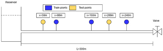
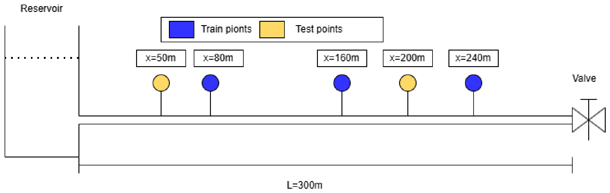
As illustrated in Figure 3, a one-dimensional pressurized pipeline system is considered, where the upstream end is connected to a reservoir, the middle section is a pipeline, and a valve is installed at the downstream end. The main parameters include the upstream reservoir head $H=50$ m, total pipe length $L=300$ m, wave speed $a=1000$ m/s, pipe diameter $D=0.05$ m, constant friction coefficient $f=0.015$, and initial flow velocity $V_0=0.412$ m/s. At the initial time, the system is assumed to be in a steady-state condition. Training data are collected at location $x_1=80,x_2=160,x_3=240$, while testing data are obtained at $x_4=50,x_5=200$, representing an extrapolation point and an interpolation point, respectively. The downstream valve is closed within the $0.1$ s, generating transient pressure waves. With a time step of $0.005$ s, a total of 2001 pressure samples are obtained within the 10 s. In addition, 30 collocation points are uniformly distributed along the pipeline. For each collocation point, 501 samples are generated over time with a time step of $0.02$ s.

Figure 3. Reservoir–pipeline–valve system.

Based on the above data construction procedure, a representative dataset for the water hammer problem is established while ensuring the accuracy of the reference solution. This dataset is used to evaluate the performance of GEAW-PINNs in terms of hyperparameter analysis, ablation studies, and parameter inversion.

3.2. Hyperparameter Analysis

In this section, a hyperparameter analysis is conducted for the proposed adaptive weighting model to evaluate the influence of different parameter settings on prediction accuracy. The investigated hyperparameters include network size, PDE loss weight, and weight update frequency. During the analysis, only one parameter is varied at a time while keeping all others fixed. The error reported in the analysis is the average error at $x=60$ m and $x=210$ m.

As shown in Table 2, for the neural network architecture, increasing the network width effectively reduces the prediction error of pressure. The smallest error, 0.0277, is achieved by the networks with depths of 6 and 8 and a width of 40. To reduce the number of parameters, we therefore choose a network depth of 6. For the PDE weight, the minimum error, 0.0279, is obtained when the weight is set to 0.5. As for the update frequency, both excessively high and low values increase the prediction error. Considering the errors in both pressure and velocity, we select an update frequency of 100.

Table 2. Relative $L^2$ error at testing points.

Hyperparameters	h	v
Depth 6 | Width 20	$1.06\times {10}^{-1}$	$3.04\times {10}^{-1}$
Depth 6 | Width 40	$2.77\times {10}^{-2}$	$7.19\times {10}^{-2}$
Depth 8 | Width 20	$3.51\times {10}^{-2}$	$9.00\times {10}^{-2}$
Depth 8 | Width 40	$2.77\times {10}^{-2}$	$7.19\times {10}^{-2}$
Depth 10 | Width 20	$2.29\times {10}^{-1}$	$6.56\times {10}^{-1}$
Depth 10 | Width 40	$2.81\times {10}^{-2}$	$7.22\times {10}^{-2}$
$w_{pde}=1$	$1.08\times {10}^{-1}$	$2.61\times {10}^{-1}$
$w_{pde}=0.5$	$2.79\times {10}^{-2}$	$7.16\times {10}^{-2}$
$w_{pde}=0.1$	$4.25\times {10}^{-2}$	$1.03\times {10}^{-1}$
$w_{pde}=0.05$	$4.14\times {10}^{-2}$	$9.92\times {10}^{-2}$
Update Frequency = 50	$2.84\times {10}^{-2}$	$7.35\times {10}^{-2}$
Update Frequency = 100	$2.79\times {10}^{-2}$	$7.16\times {10}^{-2}$
Update Frequency = 200	$2.80\times {10}^{-2}$	$7.20\times {10}^{-2}$
Update Frequency = 500	$2.74\times {10}^{-2}$	$7.25\times {10}^{-2}$

When the network widths were set to 6 and 8 with a depth of 40, the prediction errors exhibited negligible differences. Therefore, the smaller width was selected to reduce computational costs while maintaining comparable accuracy. Although an update frequency of 500 achieved a lower pressure error, the overall evaluation considering both pressure and velocity errors indicated that an update frequency of 100 yielded the best performance. Consequently, the selected hyperparameters were determined as follows:

$$\mathrm{Depth}=6,\mathrm{Width}=40,w_{pde}=0.5,\mathrm{UpdateFrequency}=100$$

(20)

3.3. Ablation Study of the Adaptive Weighting Strategy

The ablation study aims to evaluate the contribution of each component by comparing the performance of the model after removing one or more elements [37]. The training settings and the configuration of collocation points are consistent with those described in Section 3.2. In the ablation study, to avoid data leakage from the test set, the reported error is defined as the average error at $x=50$ m and $x=200$ m.

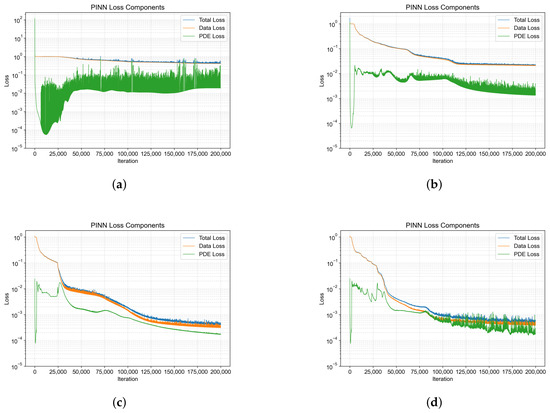
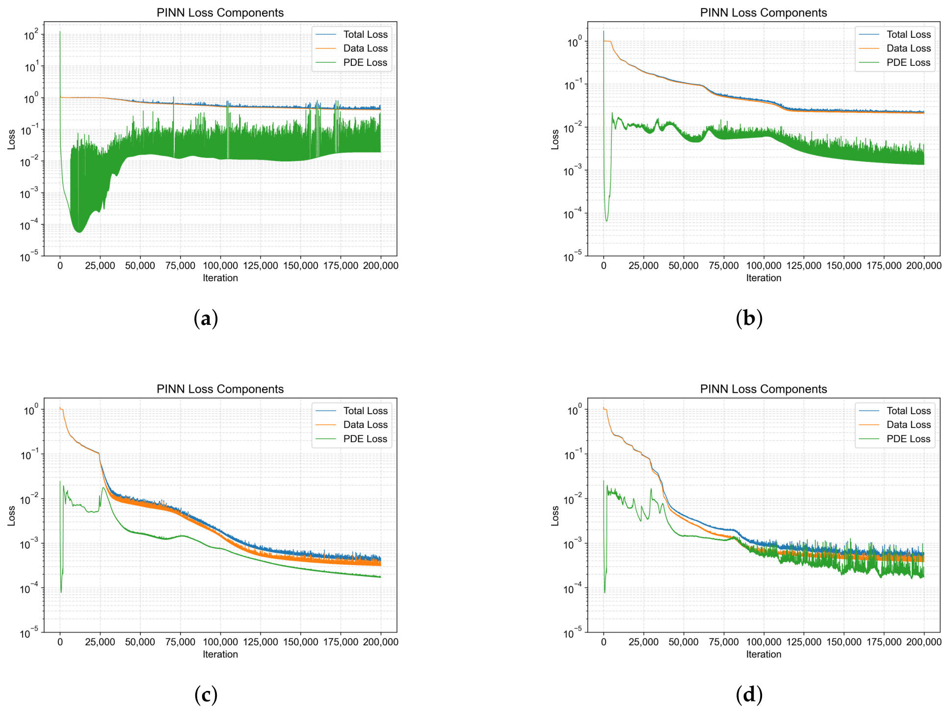
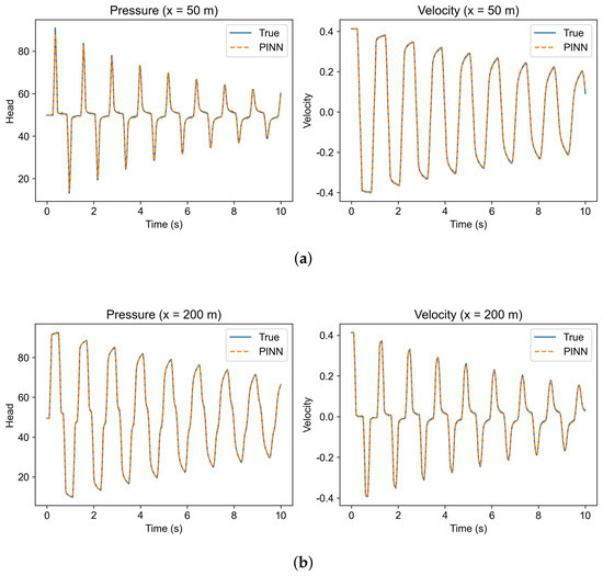
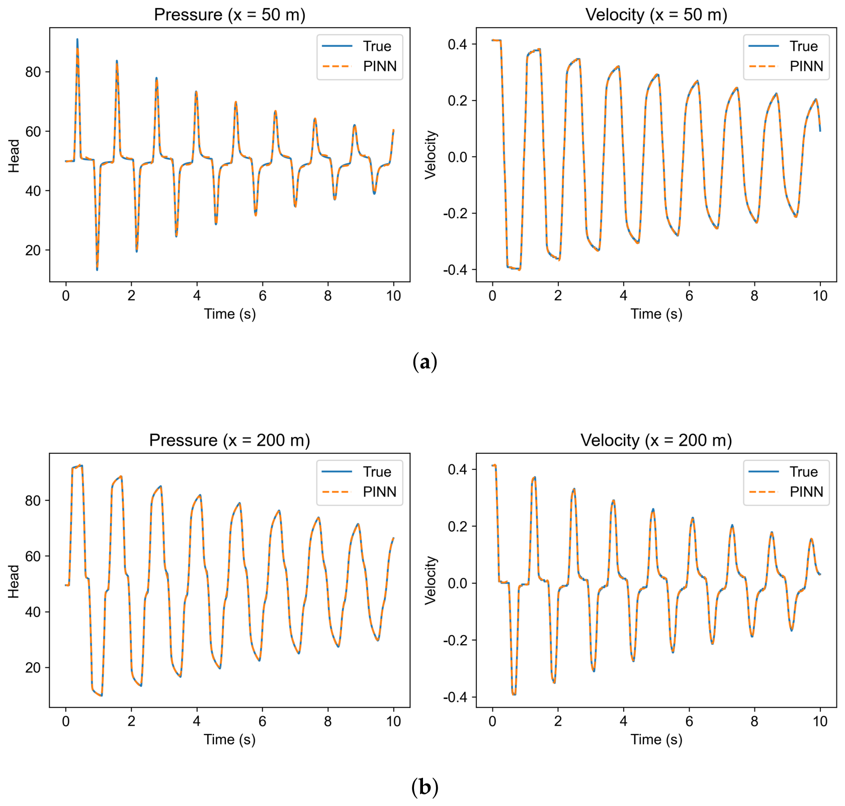
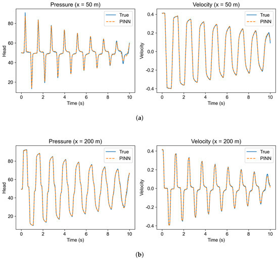
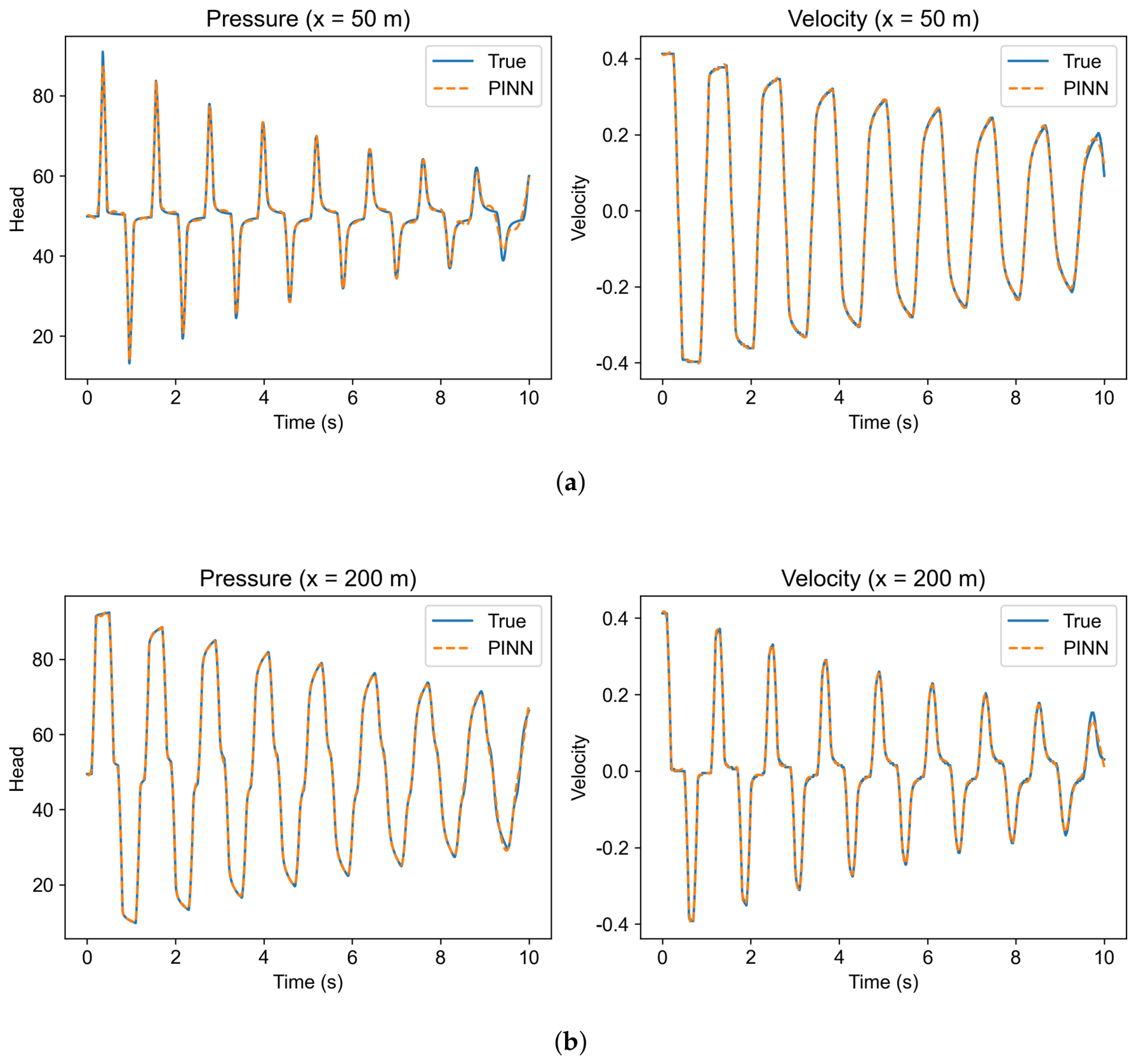
Figure 4 presents the evolution of the training losses for the standard PINN, fixed-weight PINNs, and GEAW-PINNs. For the standard PINN, the training process nearly fails, as neither the data loss nor the PDE loss decreases significantly. The corresponding prediction errors for pressure and flow velocity are 0.211 and 0.629. For the fixed-weight PINNs, the convergence behavior is highly sensitive to the choice of weights. The final loss values differ substantially under different weight settings. For GEAW-PINNs, the prediction errors are 0.00742 and 0.0183. Table 3 reports the prediction errors of the four PINN models at the observation points, as well as the model, without applying the smoothing operation during weight updating. Although the model with a fixed weight of 0.01 and the model with adaptive weighting achieve nearly the same error, GEAW-PINNs can automatically adjust the weights, thereby eliminating the need for tedious manual tuning. Moreover, the training process fails when the smoothing operation is removed during weight updating, indicating its importance for maintaining training stability. The training times for the fixed-weight PINN and the adaptive-weight PINN are 623.18 s and 623.23 s, respectively, demonstrating that the adaptive weighting strategy introduces negligible additional computational overhead. In addition, Figure 5 shows the prediction results at the test points, demonstrating that the proposed strategy can accurately predict the pressure and velocity at unseen locations.

Figure 4. Loss evolution curves: (a) fixed weight = 1, (b) fixed weight = 0.1, (c) fixed weight = 0.01, and (d) adaptive weight, respectively.

Table 3. Relative $L^2$ error at testing points.

Type	h	v
$w_{f_2}$ = 1	$2.11\times {10}^{-1}$	$6.29\times {10}^{-1}$
$w_{f_2}$ = 0.1	$4.56\times {10}^{-2}$	$1.48\times {10}^{-1}$
$w_{f_2}$ = 0.01	$6.69\times {10}^{-3}$	$1.70\times {10}^{-2}$
Without Weight Smoothing	$2.08\times {10}^{-1}$	$6.13\times {10}^{-1}$
Adaptive Weight	$7.42\times {10}^{-3}$	$1.83\times {10}^{-2}$

Figure 5. Pressure and velocity predictions at test points: (a) $x=50$ and (b) $x=200$.

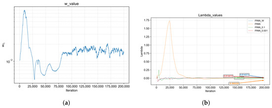
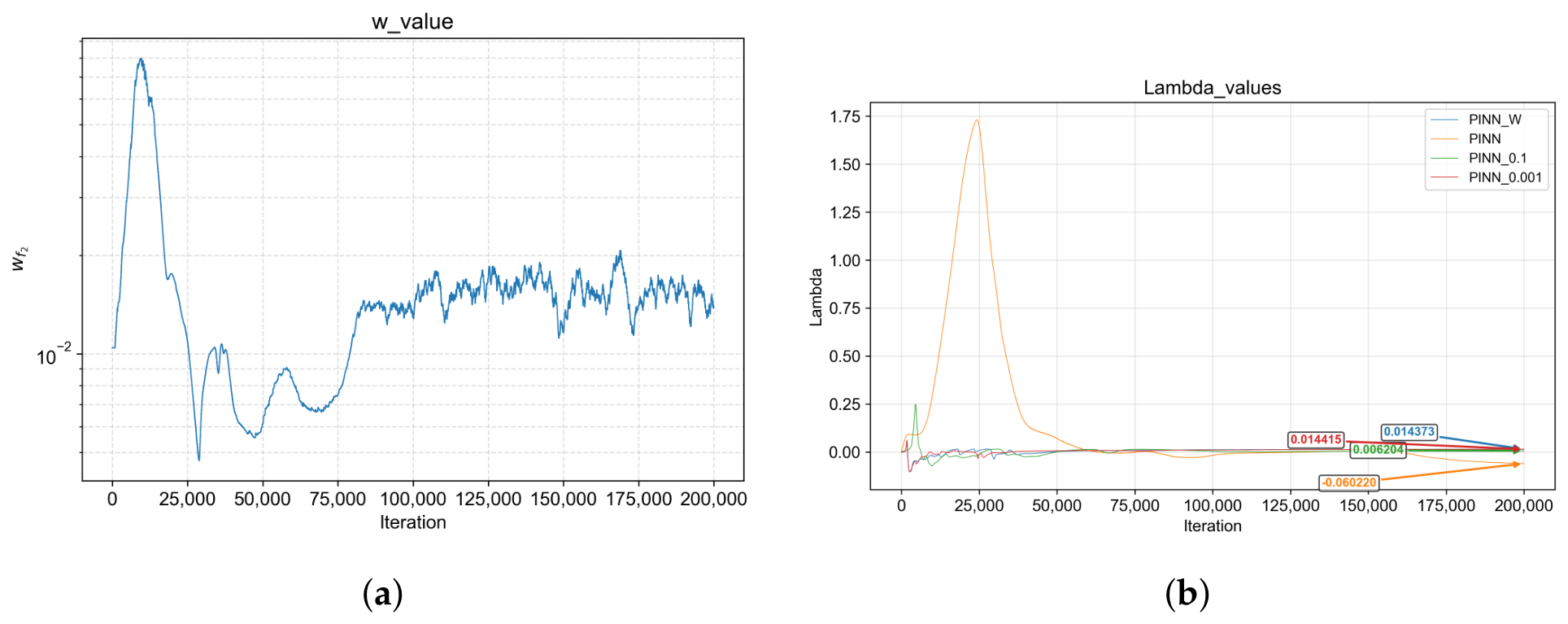
Figure 6 shows the evolution of the adaptive weights during training and the inversion results of the coefficient in the Brunone model. The final identified value is 0.01437, which is close to the reference value of 0.0128 reported by Vardy and Brown [38], indicating that the proposed GEAW-PINN strategy can automatically adjust the contributions of different physical constraints based on gradient information and is capable of identifying the Brunone parameter. It is worth noting that both the training and testing data are generated using a higher-fidelity weighted unsteady friction model, while the PINN employs the Brunone model as the governing constraint. The discrepancy between the two models explains the small deviation observed in the inversion results.

Figure 6. Comparison of $f_2$ weights (a) and trainable $\lambda$ values (b).

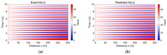
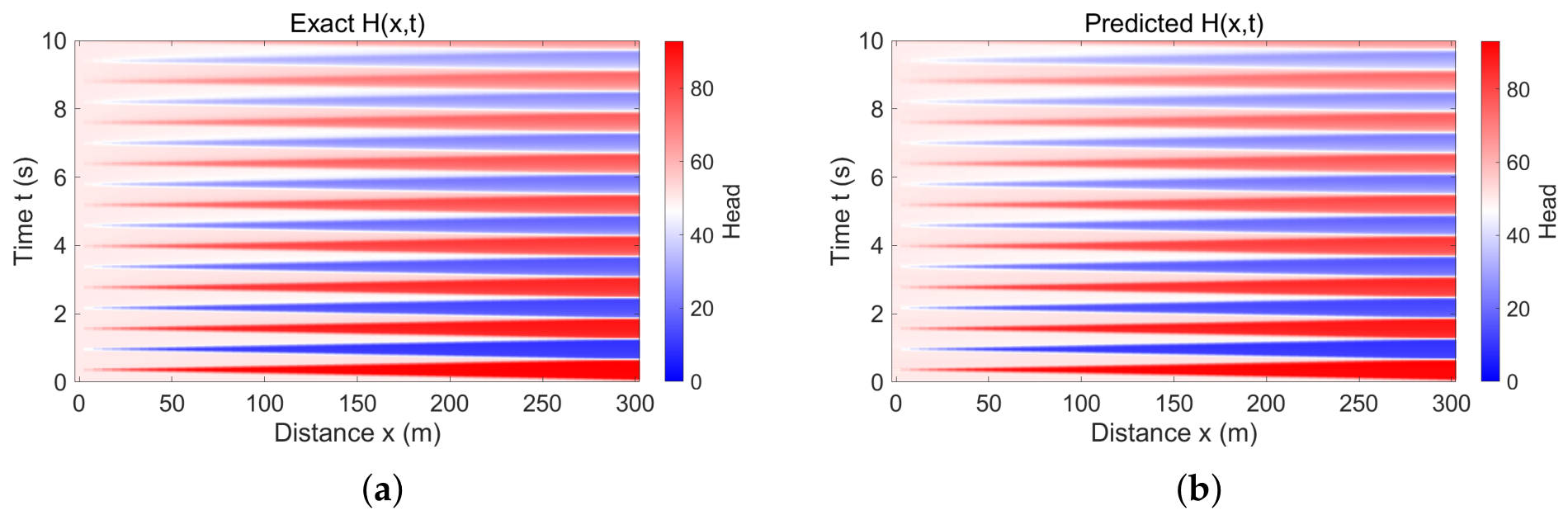
Figure 7 presents the predicted pressure field over the entire domain, where (a) shows the reference solution and (b) shows the prediction results. A high level of agreement is observed between the two, demonstrating that GEAW-PINNs can accurately capture the propagation characteristics of pressure waves during water hammer events. The average relative error near 90% of peak values is 0.0044, with a maximum relative error of 0.1107. This indicates that the model achieves high accuracy in predicting peak values, which are of particular importance in water hammer analysis.

Figure 7. Exact (a) and predicted (b) piezometric head in the global flow field.

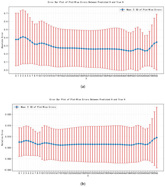
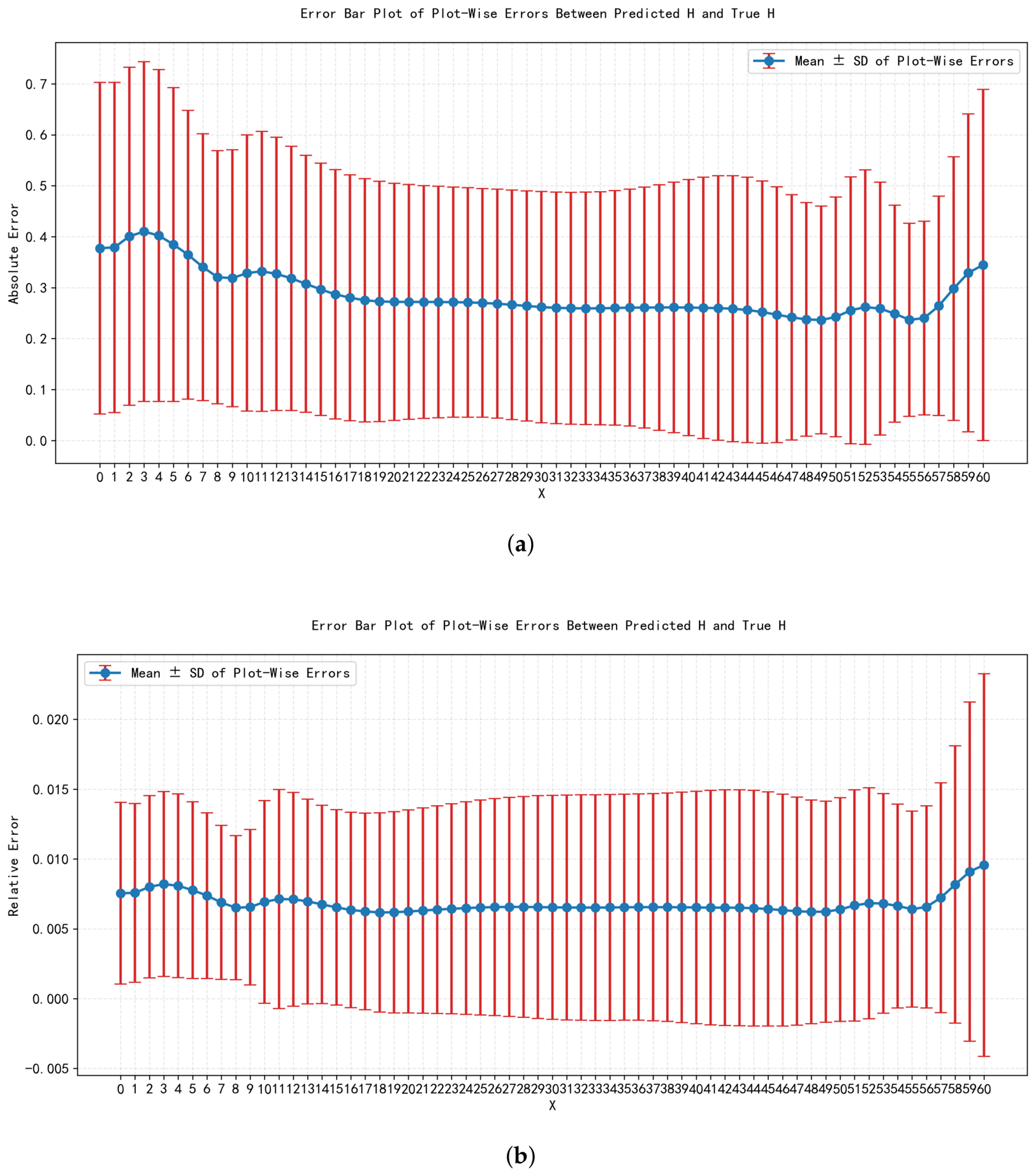
Figure 8 illustrates the mean and variance of prediction errors along the pipeline, including both absolute and relative errors. It can be observed that the prediction errors are small in the reservoir region and the middle section of the pipeline, with an average absolute error of 0.25 and a relative error of 0.008. Near the valve, the errors increase to approximately 0.35 and 0.01, accompanied by larger variance. This is mainly attributed to the strong transient behavior in the vicinity of the valve. These results indicate that GEAW-PINNs perform well across the entire pipeline, although larger errors are observed near the valve region.

Figure 8. Absolute error bar plots of predictions at each point (a), and relative error bar plots of predictions at each point (b).

Table 4 summarizes the effects of different random seeds and measurement noise on the training performance. Three random seeds (1234, 5678, and 7890) are considered. The results indicate that the choice of random seed has a negligible effect on the prediction performance, with the variances of the pressure and velocity prediction errors being only $1.1429\times {10}^{-7}$ and $6.87\times {10}^{-7}$, respectively. In addition, Gaussian noise with a signal-to-noise ratio (SNR) of 25 dB is added to the training data to simulate sensor measurements. Under this noisy condition, the variances of the pressure and velocity prediction errors increases by $9.88\times {10}^{-3}$ and $2.5\times {10}^{-2}$. The corresponding prediction results are presented in Figure 9. Although slight oscillations can be observed in the latter stage of the transient response and around the peak values, the overall prediction remains accurate, demonstrating that GEAW-PINNs possess good robustness against measurement noise.

Table 4. Relative $L^2$ error at testing points.

Type	h	v
$noise25$ dB	$1.73\times {10}^{-2}$	$3.80\times {10}^{-2}$
$seed1234$	$7.42\times {10}^{-3}$	$1.83\times {10}^{-2}$
$seed5678$	$7.60\times {10}^{-3}$	$1.90\times {10}^{-2}$
$seed7890$	$8.21\times {10}^{-3}$	$2.03\times {10}^{-2}$

Figure 9. 25 dB noisy pressure and velocity predictions at test points: (a) $x=50$ and (b) $x=200$.

Overall, the ablation study demonstrates that GEAW-PINNs can adaptively adjust the weights of different governing equations, thereby eliminating the need for laborious manual hyperparameter tuning. Moreover, it successfully identifies the Brunone coefficient through inverse estimation.

3.4. Validation on a Pipe Network System

To further evaluate the applicability of the proposed GEAW-PINN in complex hydraulic systems, a transient pipe network case presented by Yan et al. [39] was selected for validation. The benchmark data reported in the literature were adopted, and the proposed GEAW-PINN was employed to predict the transient pressure head and flow rate throughout the network. The predicted results were then compared with the corresponding reference solutions.

The network architecture, including the network width, depth, and weight update frequency, was kept consistent with those used in Section 3.2. The PDE loss weight was set to 0.001 following the configuration reported by Yan et al. [39]. Three uniformly distributed observation points in each pipe were selected as training data. The governing equations of the network are given as follows.

$$L\left(\theta \right)=L_{data}+w_{pde}{L}_{PDE}+w_{interface}{L}_{interface}$$

(21)

where $L\left(\theta \right)$, $L_{PDE}$, and $L_{interface}$ represent the total loss, the pde loss, and the interface loss, respectively. The terms $w_{pde}$ and $w_{interface}$ represent the weighting coefficients associated with the pde loss and the interface loss, respectively.

At each interface, hydraulic head continuity and flow conservation are assumed.

$$\begin{array}{c}\hfill h_j^{i{n}_1}=\dots =h_j^{i{n}_i}=h_j^{o{u}_1}=\dots =h_j^{o{u}_k}\end{array}$$

(22)

$$\begin{array}{c}\hfill {\displaystyle \sum _{j=1}^{in+ou}}{q}_j+q_{de}=0\end{array}$$

(23)

where $h_j^{i{n}_i}$ and $h_j^{o{u}_i}$ represent the pressures of the i-th incoming and outgoing pipes at the j-th interface, respectively; $q_j$ represents the total inflow and outflow rates at the junction, respectively; and $Q_{de}$ represents the water demand at the junction.

$$\begin{array}{c}\hfill \begin{array}{cc}\hfill L_{PDE}& ={\displaystyle \frac{1}{N_f}}{\displaystyle \sum _{i=1}^{N_f}}\left(f_1^2(x_f^i,t_f^i;\mathsf{\theta })+{\left(w_{f_2}{f}_2(x_f^i,t_f^i;\mathsf{\theta })\right)}^2\right)\hfill \\ \hfill L_{data}& ={\displaystyle \frac{1}{N_d}}{\displaystyle \sum _{j=1}^{N_d}}[\widehat{h}\left(x_d^j,t_d^j;\mathsf{\theta }\right)-h_d^j\left(x_d^j,t_d^j\right)\hfill \\ \hfill & +\widehat{q}\left(x_d^j,t_d^j;\mathsf{\theta }\right)-q_d^j\left(x_d^j,t_d^j\right){]}^2\hfill \\ \hfill L_{interface}& ={\displaystyle \frac{1}{N_{int}}}{\displaystyle \sum _{j=1}^{N_{int}}}{F}_3^2\left(x_{int}^j,t_{int}^j;\mathsf{\theta }\right)\hfill \end{array}\end{array}$$

(24)

$$\begin{array}{cc}\hfill F_1& =A{\displaystyle \frac{\partial \widehat{q}}{\partial t}}+\widehat{q}{\displaystyle \frac{\partial \widehat{q}}{\partial x}}+g{A}^2{\displaystyle \frac{\partial \widehat{h}}{\partial x}}+f{\displaystyle \frac{|\widehat{q}|\widehat{q}}{2D}},\hfill \end{array}$$

(25)

$$\begin{array}{cc}\hfill F_2& =A{\displaystyle \frac{\partial \widehat{h}}{\partial t}}+\widehat{q}{\displaystyle \frac{\partial \widehat{h}}{\partial x}}+{\displaystyle \frac{a^2}{g}}{\displaystyle \frac{\partial \widehat{q}}{\partial x}}+{\displaystyle \frac{a^2}{gA}}{\displaystyle \frac{\partial A}{\partial x}}\widehat{q}-\widehat{q}·sin\alpha ,\hfill \end{array}$$

(26)

$$\begin{array}{cc}\hfill F_3& ={\displaystyle \sum _{j=1}^{n_p}}\left({\widehat{h}}_j^{{\mathsf{\Psi }}_i}-{\widehat{h}}_j^{{\mathsf{\Psi }}_k}\right)+{\displaystyle \sum _{j=1}^{n_p}}\left({\widehat{q}}_j-{\widehat{q}}_{de}\right),\mathsf{\Psi }=\{in,out\}.\hfill \end{array}$$

(27)

where $(x_i,t_i)$ denotes the testing point, $u(x_i,t_i;\theta )$ represents the predicted value of the neural network, and $u_e$ is the corresponding reference value.

The $L_{PDE}$ and $L_{data}$ are computed in the same manner as in the single-pipe case, and $w_{f_2}$ is updated using the same strategy. $L_{interface}$ constraints enforce hydraulic head continuity and flow conservation.

$$L^2={\displaystyle \frac{{∥u(x_e,t_e;\theta )-U_e∥}_2}{{∥U_e∥}_2}}$$

(28)

where $(x_i,t_i)$ denotes the testing point, $u(x_i,t_i;\theta )$ represents the predicted value of the neural network, and $u_e$ is the corresponding reference value.

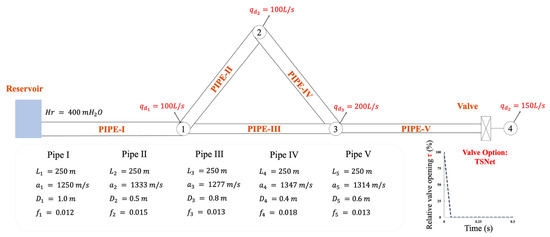
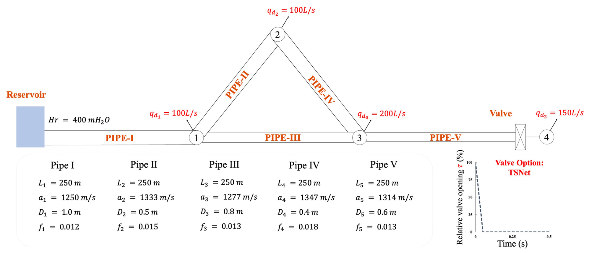
Figure 10 shows the schematic diagram of the pipe network [39].

Figure 10. The layout and conditions of pipe network schematic.

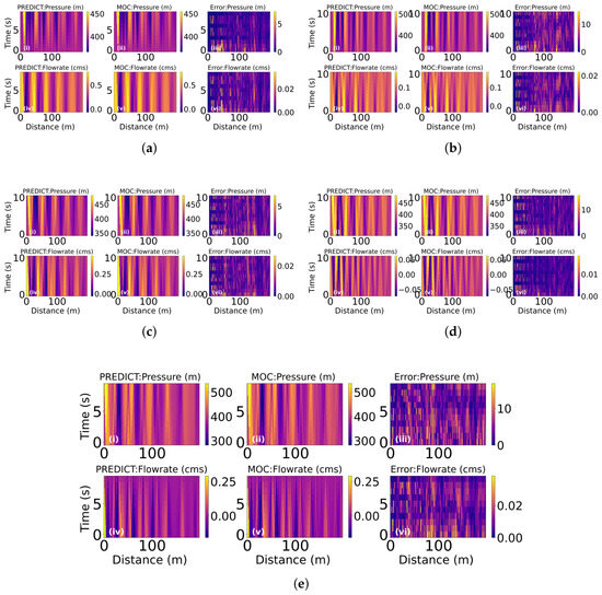
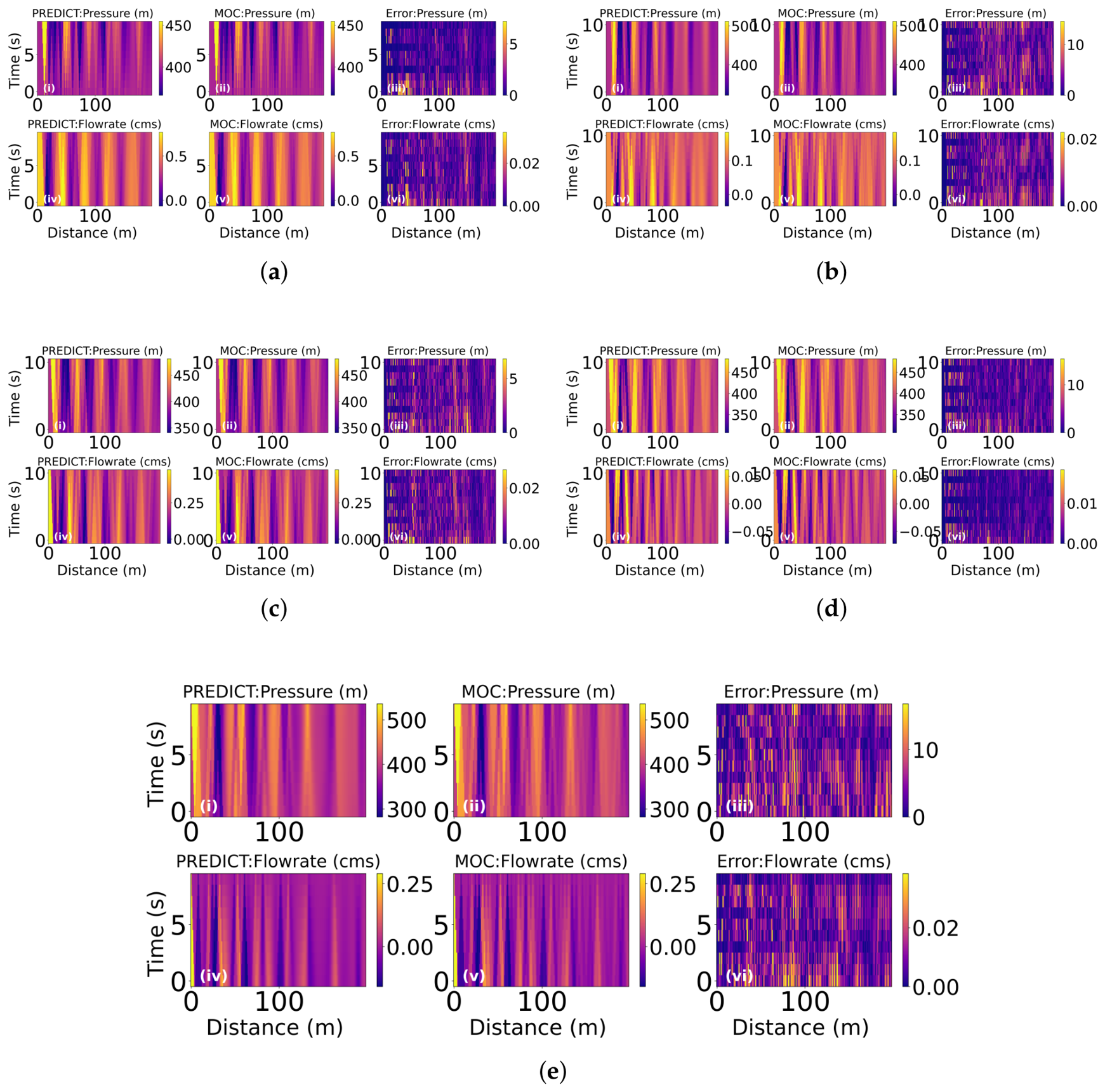
Figure 11 shows that the GEAW-PINN is capable of accurately reconstructing both pressure head and flow rate in the pipe network system.

Figure 11. Predicted pressure head, flow rate, and corresponding prediction errors for (a) Pipe 1 (i–vi), (b) Pipe 2 (i–vi), (c) Pipe 3 (i–vi), (d) Pipe 4 (i–vi), and (e) Pipe 5 (i–vi).

This case further evaluates the stability and generalization capability of the proposed gradient-based equation adaptive weighting (GEAW) strategy in complex pipe network scenarios. The results demonstrate that GEAW-PINNs maintain satisfactory convergence behavior and prediction accuracy for transient flow simulations in pipe networks, indicating that the proposed method is not only applicable to single-pipe water hammer problems but can also be effectively extended to more complex pipe network systems.

3.5. Comparison of Gradient-Based Adaptive Weighting Strategies

In this section, the proposed GEAW method is compared with the Learning Rate Annealing (LRA) [40] and Neural Tangent Kernel (NTK) methods [41]. To ensure a fair comparison, all three methods employ identical network architectures and hyperparameter settings, differing only in their weight updating strategies, which are summarized as follows.

$$\begin{array}{cc}\hfill {\widehat{\lambda }}_i\left(t\right)& ={\displaystyle \frac{\max \left\{{∥{\nabla }_{\theta }{\mathcal{L}}_{\mathsf{\Omega }}\left(t\right)∥}_1\right\}}{{∥{\nabla }_{\theta }{\mathcal{L}}_{{\{\mathsf{\Gamma },\mathsf{{\rm Y}}\}}_i}\left(t\right)∥}_1}},i\in \{1,\dots ,k\}\hfill \end{array}$$

(29)

$$\begin{array}{cc}\hfill {\lambda }_i\left(t\right)& =\alpha {\lambda }_i(t-1)+(1-\alpha ){\widehat{\lambda }}_i\left(t\right)\hfill \end{array}$$

(30)

where $max\left\{{∥{\nabla }_{\theta }{\mathcal{L}}_{\mathsf{\Omega }}\left(t\right)∥}_1\right\}$ denotes the maximum gradient of the corresponding equation, ${∥{\nabla }_{\theta }{\mathcal{L}}_{{\{\mathsf{\Gamma },\mathsf{{\rm Y}}\}}_i}\left(t\right)∥}_1$ denotes the total gradient of all equations, and $\alpha =0.9$ is a hyperparameter.

$$\begin{array}{cc}\hfill \mathcal{L}\left(\theta \right)& ={\lambda }_b{\mathcal{L}}_b\left(\theta \right)+{\lambda }_r{\mathcal{L}}_r\left(\theta \right),\hfill \end{array}$$

(31)

$$\begin{array}{cc}\hfill {\lambda }_b& ={\displaystyle \frac{{\sum }_{i=1}^{N_r+N_b}{\lambda }_i\left(n\right)}{{\sum }_{i=1}^{N_b}{\lambda }_i^{uu}\left(n\right)}}={\displaystyle \frac{\mathrm{Tr}\left(\mathit{K}\left(n\right)\right)}{\mathrm{Tr}\left({\mathit{K}}_{uu}\left(n\right)\right)}},\hfill \end{array}$$

(32)

$$\begin{array}{cc}\hfill {\lambda }_r& ={\displaystyle \frac{{\sum }_{i=1}^{N_r+N_b}{\lambda }_i\left(n\right)}{{\sum }_{i=1}^{N_r}{\lambda }_i^{rr}\left(n\right)}}={\displaystyle \frac{\mathrm{Tr}\left(\mathit{K}\left(n\right)\right)}{\mathrm{Tr}\left({\mathit{K}}_{rr}\left(n\right)\right)}}.\hfill \end{array}$$

(33)

where ${\mathcal{L}}_b\left(\theta \right)$ denotes the PDE residual loss and ${\mathcal{L}}_r\left(\theta \right)$ corresponds to boundary condition. ${\lambda }_b$ and ${\lambda }_r$ denote the weighting coefficients associated with the two terms, respectively. ${\lambda }_i\left(n\right)$, ${\lambda }_i^{uu}\left(n\right)$ and ${\lambda }_i^{rr}\left(n\right)$ are eigenvalues of $\mathit{K}\left(n\right)$, ${\mathit{K}}_{uu}\left(n\right)$, ${\mathit{K}}_{rr}\left(n\right)$ at n-th iteration.

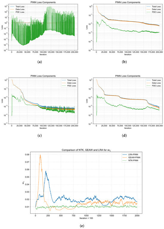
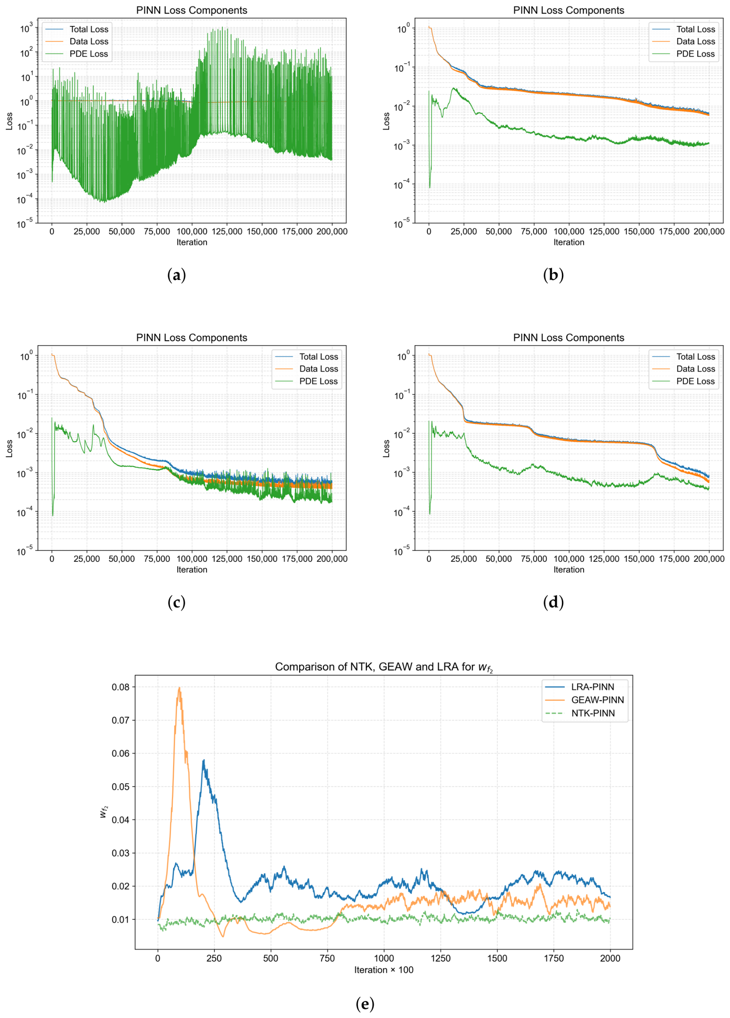
As shown in Figure 12a, the use of the maximum gradient in the numerator leads to severe oscillations in the training loss during optimization. Therefore, we replace it with the mean gradient for comparison. Figure 12b–e presents the training losses and weight evolution of the three methods for different terms. It can be observed that those methods stabilize the training process and adaptively adjust the weights according to the gradients. Moreover, the final weight values are nearly identical. Table 5 reports the prediction errors of pressure and velocity. The results show that the GEAW-PINN achieves smaller prediction errors, indicating that the GEAW-based weighting strategy could improve prediction accuracy.

Figure 12. Loss curves of LRA and GEAW, as well as plots showing weight variations throughout their training processes: (a) LRA max loss, (b) LRA mean loss, (c) GEAW loss, (d) NTK loss, and (e) weight variations.

Table 5. Relative $L^2$ error at testing points.

Type	h	v
LRA-PINN	$1.73\times {10}^{-2}$	$3.80\times {10}^{-2}$
NTK-PINN	$8.73\times {10}^{-3}$	$2.10\times {10}^{-2}$
GEAW-PINN	$7.42\times {10}^{-3}$	$1.83\times {10}^{-2}$

4. Discussion

4.1. Effectiveness of Gradient Balancing

In standard PINNs, significant differences often exist in the gradient contributions of different physical residual terms. This leads to an imbalance in their influence on parameter updates, causing the optimization process to be dominated by a particular component. The proposed adaptive weighting strategy dynamically adjusts the equation weights based on gradient magnitudes, enabling different physical constraints to contribute comparably during training and resulting in a more balanced optimization process.

Figure 2 presents the gradient curves of the two governing equations with equal weights (set to 1). As shown, both the loss and gradient exhibit strong oscillations, and a significant discrepancy in magnitude exists between the two equations. This imbalance causes the optimization process to be predominantly dominated by one equation, thereby substantially weakening the contribution of the other equation to the model training.

Figure 13 shows the comparison of gradient norms and the loss curves of the two equations in the GEAW-PINN framework. It can be observed that the losses and corresponding gradients of both equations are maintained at the same order of magnitude, while the overall fluctuations are significantly reduced. These results demonstrate that the gradient balancing strategy effectively mitigates the scale discrepancy between the two equations, enabling more balanced optimization of the physical constraints and improving the stability of the training process. Compared with the PINN proposed by Xu et al. [22], which incorporates adaptive activation functions and an unsteady friction term based on instantaneous acceleration, yielding prediction errors of $1.86\times {10}^{-2}$ and $3.61\times {10}^{-2}$ for pressure and velocity, respectively, the proposed method achieves significantly lower errors of $8.14\times {10}^{-3}$ and $1.82\times {10}^{-2}$ within the first 6 s. This corresponds to improvements of 56% and 49%, respectively, demonstrating that the GEAW-PINN can effectively enhance prediction accuracy.

Figure 13. Comparison of $f_1$ and $f_2$ gradients multiplied by the adaptive weights (a), and $f_1$ and $f_2$ loss values multiplied by the adaptive weights (b).

From an optimization perspective, the GEAW-PINN can be interpreted as a gradient-informed dynamic reweighting strategy. By regulating the influence of each loss term on parameter updates, the training process better aligns with the principles of balanced multi-objective optimization. Therefore, the GEAW-PINN shows strong applicability to PINN problems involving coupled multi-physics equations.

However, certain limitations remain. In regions with strong transient behavior, such as near the valve, the prediction error is still relatively large. This is primarily due to the rapid variations in flow conditions [42], where both pressure and velocity gradients increase significantly. Under limited data availability and finite model capacity, it remains challenging for the network to accurately capture such highly transient features.

4.2. Analysis of Parameter Inversion

Parameter inversion is one of the key tasks of PINNs in engineering applications. Under sparse observations of pressure and flow velocity, the role of physical constraints becomes increasingly important, and the balance among governing equations is particularly critical for accurate parameter identification. The experimental results demonstrate that, with the introduction of the adaptive weighting strategy, the parameter in the Brunone model converges stably to a value close to the reference solution. This indicates that the GEAW-PINN is capable of effectively leveraging limited observational data and embedded physical information to achieve accurate parameter inversion.

5. Conclusions

This study investigates the issue of training instability in Physics-Informed Neural Networks (PINNs) for hydraulic transient problems. It is shown that gradient imbalance among different governing equations can lead to optimization bias toward a dominant equation, thereby degrading prediction accuracy and physical consistency. To address this issue, a gradient-based equation adaptive weighting strategy is proposed and incorporated into the PINN framework. By dynamically adjusting the weights of different governing equations in the loss function, the proposed method ensures more balanced gradient contributions during training, enabling coordinated optimization of multiple physical constraints. As a result, accurate predictions of pressure and flow velocity in water hammer processes are achieved. And the proposed method is not only applicable to single-pipe water hammer problems but can also be effectively extended to more complex pipe network systems.

In terms of implementation, automatic differentiation is employed to compute the gradients of each governing equation, based on which adaptive weighting update strategy is constructed. A smoothing mechanism is further introduced to stabilize the weight updates during training. In addition, the network is capable of identifying the parameter in the Brunone model, providing a viable approach for parameter inversion. Comprehensive numerical experiments are conducted to validate the proposed GEAW-PINN framework, and the main findings are summarized as follows:

• Compared with the fixed-weight method, LRA, and NTK, the proposed GEAW-PINN demonstrates superior applicability to highly transient water hammer problems by automatically balancing the gradients of different governing equations. Consequently, compared with the PINN framework employing adaptive activation functions in the water hammer study by Xu et al. [22], it improves the training stability and prediction accuracy of PINNs, while maintaining a high level of agreement between the predicted results and the reference solutions.
• GEAW-PINN is capable of accurately identifying trainable parameters, indicating that it is not only suitable for predicting pressure and flow velocity, but also has strong potential for solving inverse problems.

In summary, the proposed gradient-based adaptive weighting strategy provides an effective approach for improving the stability and accuracy of PINNs in hydraulic transient problems, and offers a useful paradigm for multi-physics coupled systems.

References

- Zhou, Z.; Mu, Z.; Zhang, H.; Zhang, M.; Gu, Y.; Shi, X.; Zhao, B. Analysis and research on water hammer protection measures based on KY PIPE for long distance pumping station water transmission engineering with pump stoppage. Sci. Rep. 2025, 15, 158. [Google Scholar] [CrossRef] [Scilit] [PubMed]
- Wu, X.; Li, J.; Chen, D.; Cao, Y.; Dou, Y.; Luo, X. Tubing String Dynamics During Transient Start-Up and Shutdown in CO2 Flooding. Processes 2025, 13, 3514. [Google Scholar] [CrossRef] [Scilit]
- Wylie, E.; Streeter, V. Fluid Transients in Systems; Prentice-Hall: Englewood Cliffs, NJ, USA, 1993. [Google Scholar]
- Chaudhry, H. Applied Hydraulic Transients; Springer: New York, NY, USA, 2014; pp. 143–144. [Google Scholar]
- Zhao, M.; Ghidaoui, M.S. Godunov-type solutions for water hammer flows. J. Hydraul. Eng. 2004, 130, 341–348. [Google Scholar] [CrossRef] [Scilit]
- Raissi, M.; Perdikaris, P.; Karniadakis, G.E. Physics-informed neural networks: A deep learning framework for solving forward and inverse problems involving nonlinear partial differential equations. J. Comput. Phys. 2019, 378, 686–707. [Google Scholar] [CrossRef] [Scilit]
- Zhou, M.; Mei, G. Transfer Learning-Based Coupling of Smoothed Finite Element Method and Physics-Informed Neural Network for Solving Elastoplastic Inverse Problems. Mathematics 2023, 11, 2529. [Google Scholar] [CrossRef] [Scilit]
- Luo, D.; Mo, H.; Li, Q.; Jin, X. Solution of stress and deformation field and inversion of material parameter for gravity dams based on physics-informed neural networks. J. Comput. Sci. 2025, 89, 102613. [Google Scholar] [CrossRef] [Scilit]
- Arzani, A.; Wang, J.X.; D’Souza, R.M. Uncovering near-wall blood flow from sparse data with physics-informed neural networks. Phys. Fluids 2021, 33, 071905. [Google Scholar] [CrossRef] [Scilit]
- Zhao, B.X.; Cheng, C.M.; Peng, Z.K.; He, Q.B.; Meng, G. Hybrid Pre-Training Strategy for Deep Denoising Neural Networks and Its Application in Machine Fault Diagnosis. IEEE Trans. Instrum. Meas. 2021, 70, 3526811. [Google Scholar] [CrossRef] [Scilit]
- Xiao, Y.; Shen, C.; Zhang, W.B. Screening and prediction of metal-doped α-borophene monolayer for nitric oxide elimination. Mater. Today Chem. 2022, 25, 100958. [Google Scholar] [CrossRef] [Scilit]
- Krzystowczyk, E.; Haribal, V.; Dou, J.; Li, F. Chemical Looping Air Separation Using a Perovskite-Based Oxygen Sorbent: System Design and Process Analysis. ACS Sustain. Chem. Eng. 2021, 9, 12185–12195. [Google Scholar] [CrossRef] [Scilit]
- Kokash, H.; Khanafer, K.; Burzo, M. Machine Learning-Based Predictions of Flow and Heat Transfer Characteristics in a Lid-Driven Cavity with a Rotating Cylinder. Energies 2024, 17, 5220. [Google Scholar] [CrossRef] [Scilit]
- Tang, S.; Feng, X.; Wu, W.; Xu, H. Physics-informed neural networks combined with polynomial interpolation to solve nonlinear partial differential equations. Comput. Math. Appl. 2023, 132, 48–62. [Google Scholar] [CrossRef] [Scilit]
- Cuomo, S.; Di Cola, V.S.; Giampaolo, F.; Rozza, G.; Raissi, M.; Piccialli, F. Scientific Machine Learning Through Physics-Informed Neural Networks: Where we are and What’s Next. J. Sci. Comput. 2022, 92, 88. [Google Scholar] [CrossRef] [Scilit]
- Faroughi, S.A.; Soltanmohammadi, R.; Datta, P.; Mahjour, S.K.; Faroughi, S. Physics-Informed Neural Networks with Periodic Activation Functions for Solute Transport in Heterogeneous Porous Media. Mathematics 2024, 12, 63. [Google Scholar] [CrossRef] [Scilit]
- Jagtap, A.D.; Kawaguchi, K.; Karniadakis, G.E. Locally adaptive activation functions with slope recovery term for deep and physics-informed neural networks. Proc. R. Soc. A Math. Phys. Eng. Sci. 2020, 476, 20200334. [Google Scholar] [CrossRef] [Scilit] [PubMed]
- Bai, J.; Rabczuk, T.; Gupta, A.; Alzubaidi, L.; Gu, Y. A physics-informed neural network technique based on a modified loss function for computational 2D and 3D solid mechanics. Comput. Mech. 2023, 71, 543–562. [Google Scholar] [CrossRef] [Scilit]
- Mattey, R.; Ghosh, S. A novel sequential method to train physics informed neural networks for Allen Cahn and Cahn Hilliard equations. Comput. Methods Appl. Mech. Eng. 2022, 390, 114474. [Google Scholar] [CrossRef] [Scilit]
- Lin, S.; Chen, Y. A two-stage physics-informed neural network method based on conserved quantities and applications in localized wave solutions. J. Comput. Phys. 2022, 457, 111053. [Google Scholar] [CrossRef] [Scilit]
- Ye, J.; Do, N.C.; Zeng, W.; Lambert, M. Physics-informed neural networks for hydraulic transient analysis in pipeline systems. Water Res. 2022, 221, 118828. [Google Scholar] [CrossRef] [Scilit] [PubMed]
- Xu, Y.; Zhou, L.; Lu, Y.; Hu, Y.; Zhang, Y. Physics-informed neural networks involving unsteady friction for transient pipe flow. Water Res. 2025, 283, 123779. [Google Scholar] [CrossRef] [Scilit] [PubMed]
- Francis, J.M.; Chandhini, G.; Chamakuri, N. An adaptive residual-structured and scheduled loss weighting framework for enhancing physics-informed neural networks in solving partial differential equations. Commun. Nonlinear Sci. Numer. Simul. 2026, 153, 109531. [Google Scholar] [CrossRef] [Scilit]
- Zhang, S.; Zhang, C.; Wang, B. A physics-informed neural network for aiding the acquisition of high-fidelity multiphysics fields in gas-phase combustion reacting flows without pre-training. Phys. Fluids 2025, 37, 097135. [Google Scholar] [CrossRef] [Scilit]
- Zhao, Z.; Ren, B. PINNs with hybrid residual-driven adaptive sampling and weighted loss for the (2+1)-dimensional gpKP equation. Phys. Lett. A 2025, 561, 130998. [Google Scholar] [CrossRef] [Scilit]
- Bischof, R.; Kraus, M.A. Multi-Objective Loss Balancing for Physics-Informed Deep Learning. Comput. Methods Appl. Mech. Eng. 2025, 439, 117914. [Google Scholar] [CrossRef] [Scilit]
- Wang, Y.; Shi, L.; Hu, X.; Song, W.; Wang, L. Multiphysics-Informed Neural Networks for Coupled Soil Hydrothermal Modeling. Water Resour. Res. 2023, 59, e2022WR031960. [Google Scholar] [CrossRef] [Scilit]
- Brunone, B.; Golia, U.M.; Greco, M. Modeling of Fast Transients by Numerical Methods. In Proceedings of the International Conference on Hydraulic Transients with Water Column Separation; IAHR-Group: Madrid, Spain, 1991; pp. 273–280. [Google Scholar]
- Vardy, A.; Brown, J. Efficient Approximation of Unsteady Friction Weighting Functions. J. Hydraul. Eng. 2004, 130, 1097–1107. [Google Scholar] [CrossRef] [Scilit]
- Covas, D.; Stoianov, I.; Mano, J.F.; Ramos, H.; Graham, N.; Maksimovic, Č. The dynamic effect of pipe-wall viscoelasticity in hydraulic transients. Part II—Model development, calibration and verification. J. Hydraul. Res. 2005, 43, 56–70. [Google Scholar] [CrossRef] [Scilit]
- Vardy, A.E.; Brown, J.M. Approximation of Turbulent Wall Shear Stresses in Highly Transient Pipe Flows. J. Hydraul. Eng. 2007, 133, 1219–1228. [Google Scholar] [CrossRef] [Scilit]
- Apollonio, C.; Covas, D.; De Marinis, G.; Leopardi, A.; Ramos, H. Creep functions for transients in HDPE pipes. Urban Water J. 2014, 11, 160–166. [Google Scholar] [CrossRef] [Scilit]
- Evangelista, S.; Leopardi, A.; Pignatelli, R.; De Marinis, G. Hydraulic Transients in Viscoelastic Branched Pipelines. J. Hydraul. Eng. 2015, 141, 04015016. [Google Scholar] [CrossRef] [Scilit]
- Kingma, D.P.; Ba, J. Adam: A Method for Stochastic Optimization. arXiv 2017, arXiv:1412.6980. [Google Scholar] [CrossRef] [Scilit]
- Liu, D.C.; Nocedal, J. On the limited memory BFGS method for large scale optimization. Math. Program. 1989, 45, 503–528. [Google Scholar] [CrossRef] [Scilit]
- Boyd, S.; Vandenberghe, L. Convex Optimization; Cambridge University Press: New York, NY, USA, 2004. [Google Scholar]
- Girshick, R.; Donahue, J.; Darrell, T.; Malik, J. Rich feature hierarchies for accurate object detection and semantic segmentation. In Proceedings of the IEEE Conference on Computer Vision and Pattern Recognition; IEEE: New York, NY, USA, 2014; pp. 580–587. [Google Scholar]
- Vardy, A.E.; Brown, J.M. Transient, turbulent, smooth pipe friction. J. Hydraul. Res. 1995, 33, 435–456. [Google Scholar] [CrossRef] [Scilit]
- Yan, H.; Li, S.; Tian, W.; Wang, J.; Li, F.; Duan, H.; Tao, T.; Xin, K. A Hybrid Model Coupling Data and Hydraulic Transient Laws for Water Distribution Systems. Water Resour. Res. 2025, 61, e2023WR036641. [Google Scholar] [CrossRef] [Scilit]
- Wang, S.; Teng, Y.; Perdikaris, P. Understanding and mitigating gradient pathologies in physics-informed neural networks. arXiv 2020, arXiv:2001.04536. [Google Scholar] [CrossRef] [Scilit]
- Wang, S.; Yu, X.; Perdikaris, P. When and why PINNs fail to train: A neural tangent kernel perspective. J. Comput. Phys. 2022, 449, 110768. [Google Scholar] [CrossRef] [Scilit]
- Li, Z.; Jin, J.; Pan, Z.; Sun, J.; Geng, K.; Qiao, Y. Impact of Branch Pipe Valve Closure Procedures on Pipeline Water Hammer Pressure: A Case Study of Xinlongkou Hydropower Station. Appl. Sci. 2025, 15, 897. [Google Scholar] [CrossRef] [Scilit]
Disclaimer/Publisher’s Note: The statements, opinions and data contained in all publications are solely those of the individual author(s) and contributor(s) and not of MDPI and/or the editor(s). MDPI and/or the editor(s) disclaim responsibility for any injury to people or property resulting from any ideas, methods, instructions or products referred to in the content. |
© 2026 by the authors. Licensee MDPI, Basel, Switzerland. This article is an open access article distributed under the terms and conditions of the Creative Commons Attribution (CC BY) license.