


Abstract
Rainfall input, as the primary driver of distributed hydrological models, can be derived from rain gauge observations or weather radar quantitative precipitation estimates (QPEs). While radar–gauge fusion products offer high-resolution spatial rainfall information, their comparative performance against traditional gauge-interpolated rainfall in small regulated catchments remains insufficiently understood. This study conducted a systematic comparison of radar–gauge fusion and gauge-interpolated rainfall inputs for flood simulation in the Yongtai pumped-storage hydropower catchment (∼60.5 km2) in Fujian Province, China. Using the physically based Liuxihe distributed hydrological model, six typical flood events (2023–2025) encompassing various magnitudes and hydrograph patterns were simulated. Model parameters were optimized via particle swarm optimization, and simulation accuracy was evaluated using NSE, KGE, peak relative error (PRE), and absolute peak time error (APTE). Rainfall spatial variability was quantified using the coefficient of variation (CV) and information entropy (H). Results showed that both rainfall inputs achieved generally acceptable simulation accuracy for most events after parameter optimization, with APTE within 1 h and PRE mostly below 15%, although event-to-event differences remained evident. Radar–gauge rainfall exhibited consistently higher CV (+34.1%) and H (+84.4%) than gauge-interpolated rainfall across all events, indicating greater spatial variability and entropy-derived spatial information diversity. Under the independent-calibration framework, the radar–gauge rainfall-driven configuration showed better metrics for the investigated multi-peak and localized intense-rainfall events; however, it systematically underestimated rainfall magnitude under weak rainfall conditions, leading to degraded peak simulation (PRE of 54.1% vs. 14.3%). These differences reflect the combined effects of rainfall input and separately optimized parameter sets and should not be interpreted as evidence of the intrinsic superiority of one rainfall product. Based on these event-limited findings, a “radar-primary, gauge-auxiliary” multi-source strategy is suggested as a potential operational option for small pumped-storage catchments to balance spatial representativeness and observational reliability.
1. Introduction
Flood forecasting is a core component of non-structural flood mitigation systems, and its accuracy directly influences the timeliness and effectiveness of flood control decisions and emergency responses. Distributed hydrological models, which discretize catchment surfaces into grid cells to represent spatial heterogeneity, have become essential tools for flood simulation in small and medium-sized catchments [1,2,3]. However, rainfall—the most critical driving input for these models—must be reconstructed from discrete point observations (rain gauges) or remote sensing retrievals (radar) into continuous spatial fields through interpolation or inversion algorithms. This reconstruction process may introduce representation errors and rainfall-input uncertainty [4,5], which propagate through nonlinear rainfall–runoff processes and ultimately affect the accuracy and reliability of flood simulations [6,7,8].
In operational flood forecasting, two primary rainfall data sources are commonly used: ground-based rain gauge observations and weather radar quantitative precipitation estimates (QPEs). Rain gauges provide high point-accuracy measurements but have limited spatial representativeness, particularly when the gauge network is sparse and unable to capture the spatial heterogeneity of rainfall fields [9,10]. In contrast, radar rainfall products offer gridded rainfall information at high spatiotemporal resolutions, providing significant advantages in compensating for the spatial coverage limitations of rain gauge networks [11]. However, radar QPE may suffer from systematic biases related to Z–R relationship uncertainty, ground clutter, beam blockage, and signal attenuation, with accuracy being particularly uncertain under complex terrain or weak rainfall conditions [12]. Therefore, quantitatively understanding the spatial variability characteristics and uncertainty sources of different rainfall input types is essential for maximizing the decision-support capability of multi-source observations and distributed models.
Pumped-storage hydropower catchments represent a special class of small watersheds characterized by significant engineering regulation and rapid hydrological response. These catchments transfer water between upper and lower reservoirs during pumping and power-generation cycles, substantially altering natural hydrological processes. In the Yongtai catchment, the lower reservoir is located near Lingxia Village and downstream residential and infrastructure areas; therefore, inflow forecasting also supports local flood-prevention decisions and emergency preparedness. Such catchments are typically small in area (often <100 km2), located in mountainous terrain with flashy hydrological regimes, and exhibit strong spatial heterogeneity in rainfall, with flood events characterized by rapid onset and short duration. Furthermore, the relatively short operational history of these facilities limits the availability of observed flood data for model calibration and validation, constraining the applicability of traditional data-driven models. Physics-based distributed hydrological models, which require fewer historical flood data for parameter estimation, are better suited for such data-scarce and spatially heterogeneous catchments. Given the rapid growth of pumped-storage hydropower in China and globally, improved flood forecasting in these catchments has practical significance for flood risk management and renewable energy system reliability.
Previous studies have compared alternative precipitation inputs for hydrological modeling, including radar, gauge, and gridded precipitation products [13,14,15,16], but most have focused on larger basins or urban catchments, with limited attention given to small, regulated pumped-storage catchments [17]. Moreover, existing comparisons primarily evaluate simulation accuracy directly, without systematically quantifying and explaining performance differences from the perspective of rainfall spatial variability [18,19,20]. Recent work by Huang and Chen [21] investigated the impact of rain gauge density on flood forecasting performance using the Liuxihe model in a mesoscale catchment, demonstrating that model performance exhibits threshold behavior as gauge density decreases. In our previous study [22], we developed a Liuxihe model-based flood forecasting approach for the same Yongtai pumped-storage catchment using only rain gauge observations, confirming the applicability of the distributed hydrological model for flood simulation in such regulated small catchments. Building upon that work, the present study further incorporates radar–gauge fusion rainfall data to systematically compare the performance and spatial variability characteristics of the two rainfall inputs.
The objectives of this study are therefore to: (1) evaluate the flood simulation accuracy of the Liuxihe distributed hydrological model driven by radar–gauge fusion and gauge-interpolated rainfall inputs in the Yongtai pumped-storage catchment; (2) quantify the spatial variability differences between the two rainfall data sources using CV and information entropy; (3) analyze the relationship between rainfall spatial characteristics and flood simulation performance differences; and (4) provide practical guidance for rainfall input selection in operational flood forecasting for small pumped-storage catchments.
2. Study Area and Data
2.1. Study Area
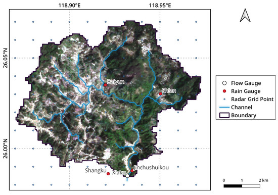
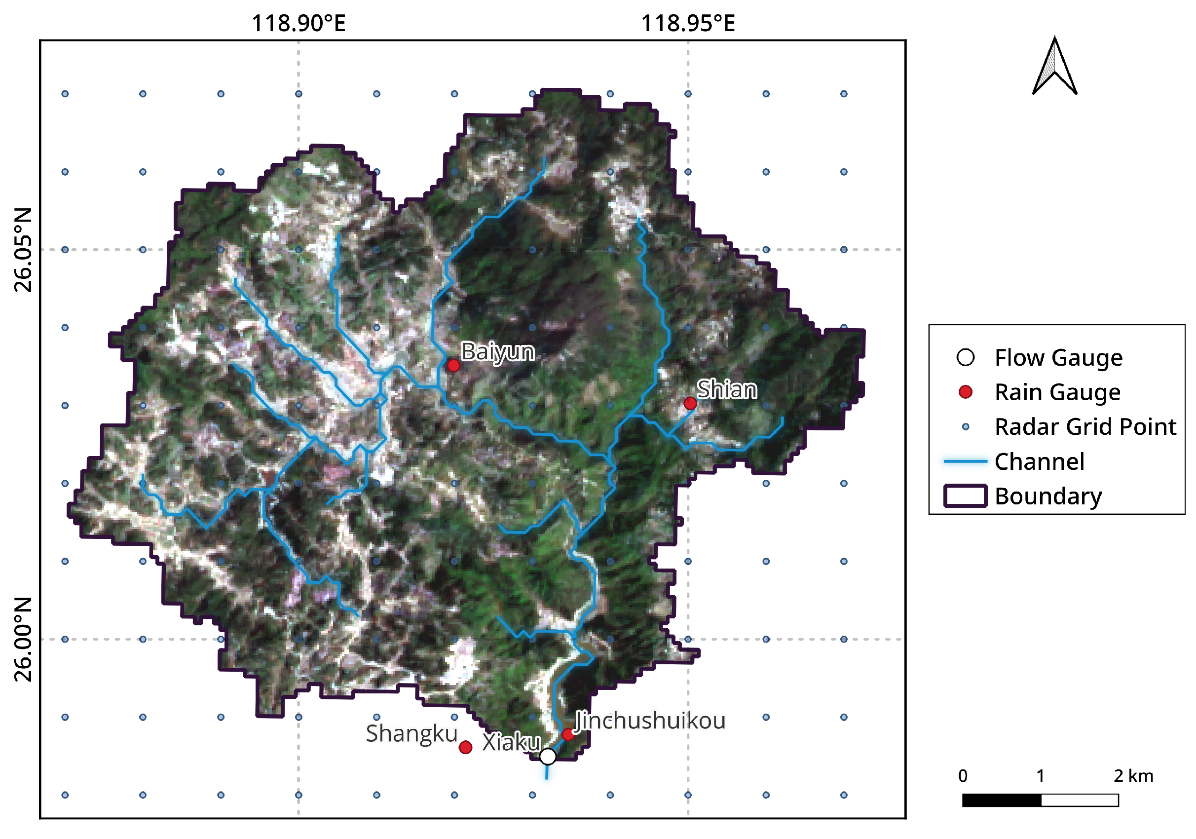
The Yongtai pumped-storage hydropower catchment is located in Baiyun Township, Yongtai County, Fuzhou City, Fujian Province, southeastern China (Figure 1). Situated in a coastal mountainous region influenced by the East Asian monsoon, the catchment receives abundant rainfall with strong spatiotemporal variability. The upper and lower reservoirs are both located within the Baiyun Stream watershed, a first-order tributary of the Yuxi River basin, with the lower reservoir dam sited at Lingxia Village in the middle reaches of Baiyun Stream. The catchment covers an area of approximately 60.5 km2, with a main channel length of approximately 18.2 km. The terrain is predominantly mountainous, characterized by deeply incised channels, steep banks, and high gradients. The riverbed consists mainly of gravel and cobbles. Baseflow is low during non-flood seasons, whereas runoff generation and concentration are rapid under intense rainfall, reflecting typical mountainous stream behavior.
Figure 1.
Overview of the Yongtai pumped-storage hydropower catchment in Yongtai County, Fuzhou City, Fujian Province, China (adapted from [22]). The remote-sensing image is a Landsat 8 RGB composite (RGB = Bands 4-3-2), showing the terrain and land-cover characteristics within the catchment. Maps were produced using QGIS 3.40.11 and Python 3.12 (Matplotlib 3.11.1).
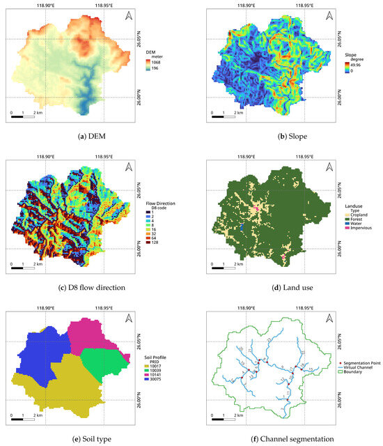
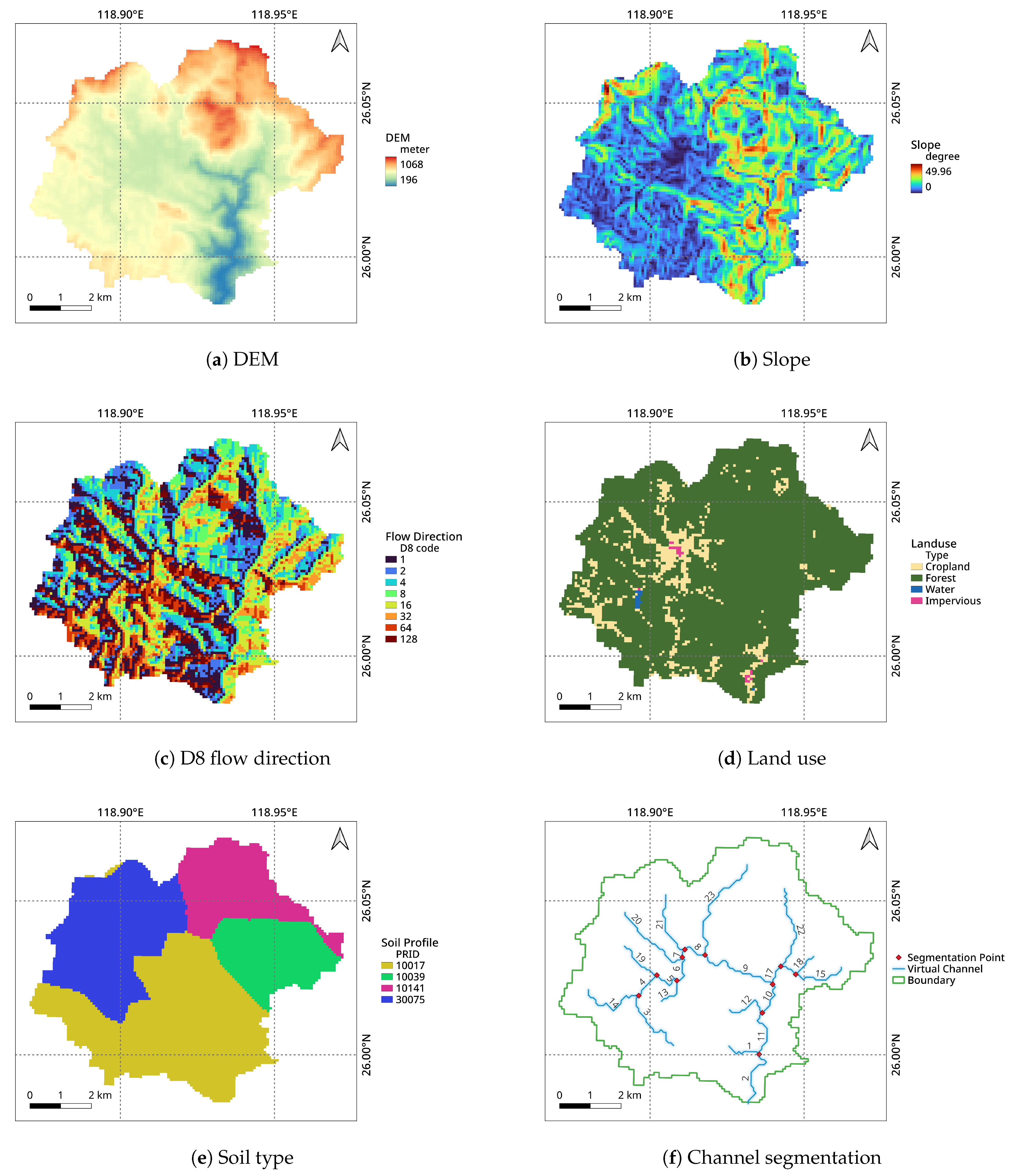
Due to the operational requirements of the pumped-storage power station and the flood-prevention needs of downstream settlements, inflow forecasting for the lower reservoir is needed to support reservoir regulation, operational safety, and local flood response. The catchment is equipped with up to five rain gauges, with the Baiyun station at the catchment center serving as the primary station, and a hydrological station at the lower reservoir monitoring water level. During 2023, the two operational gauges (Baiyun and Xiaku) provided a basic upstream–downstream coverage for this small catchment. Since the station became operational in 2023, six typical flood events have been recorded, providing a basis for hydrological model construction and calibration. The description of the study area, the catchment overview map (Figure 1), and the underlying surface data (Figure 2) are adapted from our previous study [22].
Figure 2.
Underlying surface data for Liuxihe model construction in the Yongtai pumped-storage hydropower catchment (adapted from [22]). Maps were produced using QGIS 3.40.11.
2.2. Underlying Surface Data
The construction of a distributed hydrological model requires fundamental data characterizing the physical properties of the catchment surface. The digital elevation model (DEM) used in this study is the SRTM DEM V4 dataset [23] with a spatial resolution of 90 m. The catchment elevation ranges from 196 to 1068 m, with deeply incised channels and pronounced topographic relief. Land use data were obtained from the 30 m annual land cover dataset of China [24]; the catchment is predominantly forested (88.7% coverage). Soil type data were derived from the SOTER China soil database [25], comprising four soil types. Soil hydraulic parameters were estimated using the pedotransfer functions of Saxton and Rawls [26]. River channel characteristics were measured and estimated from remote sensing imagery.
2.3. Flood Event and Rainfall Data
Flood event data were provided by Fujian Yongtai Mintou Pumped-Storage Co., Ltd. (Fuzhou, China). Six typical flood events recorded since station operation began in 2023 were compiled at an hourly temporal resolution. Table 1 summarizes the characteristics of these events. In terms of peak discharge magnitude, the events span small, medium, and large categories. Event durations range from 41 h to 105 h, covering both short-duration flash floods and longer-duration sustained events. Hydrograph patterns include single-peak events (27 July 2023, 4 September 2023, 21 September 2024, 22 May 2025) and multi-peak events (24 July 2024, 20 July 2025), enabling a comprehensive evaluation of model performance across diverse flood conditions.
Table 1.
Summary of flood events in the Yongtai pumped-storage catchment.
Rainfall data were obtained from two sources:
- 1.
- Rain gauge observations: Provided by Fujian Yongtai Mintou Pumped-Storage Co., Ltd. Only two gauges (Baiyun and Xiaku) were available in 2023; two additional gauges (Jinchushuikou and Shangku) were added in 2024. Continuous rainfall grids matching the model resolution were generated from discrete gauge observations using the Thiessen Polygon interpolation method.
- 2.
- Radar–gauge fusion product: Provided by the Fujian Meteorological Service Center. This product is an operational quantitative precipitation estimation (QPE) rainfall analysis product generated by combining weather-radar-based precipitation estimates from surrounding radar stations with quality-controlled automatic rain-gauge observations. Radar QPE first estimates rainfall intensity from the radar reflectivity factor and, where conditions permit, dual-polarization radar variables through empirical or locally adjusted precipitation-estimation relationships. Rain-gauge observations are then used to constrain and correct the radar-estimated rainfall field, including bias correction and spatial correction, so as to reduce the uncertainty of radar-only retrievals under different precipitation types and complex terrain conditions. The product used in this study was further bias-corrected for the Yongtai catchment area and was provided with approximately 1 km spatial resolution as hourly gridded rainfall fields. Therefore, this radar–gauge fusion product preserves the spatial continuity of radar rainfall while incorporating ground-observation constraints on rainfall magnitude.
Table 2 lists the total rainfall amounts for the two input types across all six events. Total rainfall ranges from 51.1 mm to 320.9 mm, encompassing weak, moderate, and heavy rainfall conditions, thus providing a suitable data basis for comparing the performance of the two rainfall inputs under diverse rainfall characteristics.
Table 2.
Rainfall data for flood events in the Yongtai pumped-storage catchment.
3. Methods
3.1. Liuxihe Model
The Liuxihe model is a physically based distributed hydrological model developed by Chen et al. [27,28], primarily designed for hourly flood forecasting in small and medium-sized catchments. The model discretizes the catchment horizontally into hillslope, channel, and reservoir grid cells based on DEM, land use, and soil type data. Each cell type is associated with specific runoff generation and flow routing computations.
In runoff generation, net rainfall is computed from rainfall input minus actual evapotranspiration. For hillslope cells, an infiltration coefficient controls the proportion of rainfall that contributes to runoff; when rainfall intensity exceeds the soil hydraulic conductivity, excess infiltration runoff is generated. For channel cells, net rainfall directly becomes runoff. Flow routing is performed using a simplified Saint-Venant equation solved via the Newton–Raphson iterative method to compute discharge at each cell, ultimately yielding the simulated hydrograph at the catchment outlet. Detailed model theory and methodology can be found in the relevant literature [27,28].
The model was constructed at a spatial resolution of 90 m. The parameter set used in model construction includes three groups: (1) evapotranspiration-related parameters, including field capacity, wilting water content, potential evaporation rate, and evaporation coefficient; (2) runoff-generation parameters, including saturated water content, soil thickness, saturated hydraulic conductivity, initial soil moisture content, and soil property parameters; and (3) routing-related parameters, including flow direction, grid-cell slope, Manning roughness coefficient, soil infiltration coefficient, channel bottom width, channel bed slope, and channel side slope. Except for initial soil moisture content, these parameters were derived or fixed from DEM, soil type, land use, remote sensing imagery, and empirical reference values. Channel bottom width was estimated by measuring three cross-sections (upstream, middle, and downstream) for each virtual channel segment from remote sensing imagery and taking the average.
3.2. Parameter Optimization
The Liuxihe model employs the particle swarm optimization (PSO) algorithm [29] for automatic parameter calibration [28]. PSO is a heuristic stochastic optimization method inspired by swarm intelligence, combining global search capability with computational efficiency. In the calibration hydrograph, “Ini” denotes simulations using the initial parameter set, while “Opt” denotes simulations using the optimized parameter set obtained through PSO calibration; “Gauge” and “Radar” indicate gauge-interpolated and radar–gauge rainfall inputs, respectively.
Given that the observed discharge data were derived from reservoir stage–discharge rating curves and exhibit some irregular fluctuations, a KGE-based objective function was adopted to enhance optimization stability:
KGE integrates correlation, bias, and variability components and is less sensitive to local fluctuations, making it more suitable for discharge sequences with irregular perturbations [30].
The maximum number of PSO iterations was set to 50. The swarm size was set to 14, the inertia weight to 0.73, and both the cognitive learning factor and social learning factor to 1.4962. Parameter values were constrained within the range times their initial physically based estimates to ensure physically meaningful and stable optimization results.
The PSO optimization was applied within physically constrained parameter ranges, with initial soil moisture content treated as the primary event-sensitive adjustable parameter and the remaining parameters constrained by the catchment physical data and empirical reference values described above. Spatial resolution differences among input datasets were handled by resampling all rainfall inputs to the 90 m model grid (consistent with the DEM resolution) using nearest-neighbor interpolation, ensuring a consistent spatial discretization for comparison.
To ensure a consistent experimental framework for fair comparison between the two rainfall inputs, the gauge-interpolated rainfall parameters were re-optimized using the same objective function and PSO configuration as the radar–gauge rainfall input. Although the authors’ previous study [22] reported gauge-based flood simulation results for the same catchment using a different optimization setup, the simulation accuracy obtained in this study is closely comparable, with only minor differences attributable to the unified optimization protocol. This consistency indicates that the unified optimization setup yields comparable calibration-event results, but it does not remove the limitations of single-event calibration discussed in Section 5.4.
3.3. Flood Simulation Evaluation Metrics
Five evaluation metrics were employed to quantitatively assess flood simulation accuracy:
- 1.
- Nash–Sutcliffe Efficiency (NSE): Reflects the overall agreement between simulated and observed hydrographs [31].
- 2.
- Kling–Gupta Efficiency (KGE): Integrates correlation coefficient, mean ratio, and standard deviation ratio [32].
- 3.
- Correlation Coefficient (R): Measures the linear correlation between simulated and observed discharge.
- 4.
- Peak Relative Error (PRE): Quantifies the relative deviation in peak discharge magnitude.
- 5.
- Absolute Peak Time Error (APTE): Quantifies the timing error of the simulated peak.
3.4. Rainfall Spatial Variability Metrics
Two metrics were adopted to quantitatively characterize spatial variability differences between the two rainfall inputs:
3.4.1. Coefficient of Variation (CV)
The coefficient of variation is the ratio of the standard deviation to the mean, describing the relative dispersion of rainfall grid values:
Higher CV values indicate stronger spatial dispersion of rainfall, greater differences among grid cells, and more pronounced spatial heterogeneity [33]. The event-weighted mean CV was computed using the total rainfall amount at each time step as the weight.
3.4.2. Information Entropy (H)
Information entropy, derived from information theory, measures the complexity and randomness of rainfall spatial distribution [34,35,36]:
where denotes the proportion of rainfall grid cells belonging to the i-th class or bin, and m is the total number of classes or bins. In this study, information entropy was used as a diagnostic measure of spatial information diversity and pattern complexity. A higher entropy value indicates a more spatially diverse and less uniform rainfall pattern under the specified classification scheme. For the event-weighted hourly rainfall entropy, rainfall intervals were classified based on physical rainfall intensity categories (trace: <0.1 mm; light: 0.1–2 mm; moderate: 2–10 mm; heavy: 10–25 mm; rainstorm: 25–50 mm; extreme: >50 mm) to enhance the hydrological interpretability of the metric. For accumulated rainfall fields, entropy was computed using an equal-width binning procedure across the accumulated rainfall value range because event-total rainfall no longer corresponds directly to instantaneous rainfall-intensity categories. The same grid extent, spatial resolution, binning procedure, and logarithm convention were applied to both rainfall inputs. No normalization was used to convert H to a 0–1 index. Because the absolute magnitude of H depends on class selection and discretization, H is interpreted only as a relative diagnostic metric under this common calculation framework and not as a direct indicator of rainfall-estimation accuracy.
3.5. Experimental Design
The experimental procedure was as follows: (1) the Liuxihe model was driven separately by gauge-interpolated rainfall and radar–gauge fusion rainfall; (2) the first recorded typical flood event (27 July 2023) was used to optimize model parameters via PSO, yielding two parameter sets; (3) the optimized parameters were applied to the remaining five validation flood events, and simulation accuracy was compared between the two rainfall inputs; and (4) the spatial variability of each rainfall input was quantified using CV and information entropy for each flood event, and the relationship between spatial variability and flood simulation performance differences was analyzed. The event 27 July 2023 was selected as the calibration event because it is the first recorded event with a moderate peak discharge (86 m3/s), covers a wide range of flow conditions, and its single-peak pattern with well-defined rising and falling limbs provides representative information for parameter estimation. This single-event calibration strategy is also consistent with previous Liuxihe model applications showing that PSO-based calibration of physically constrained parameters can obtain stable parameter sets from representative flood events [22,28].
4. Results
4.1. Parameter Optimization Results
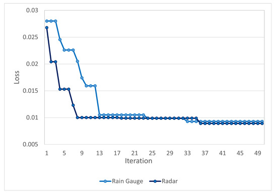
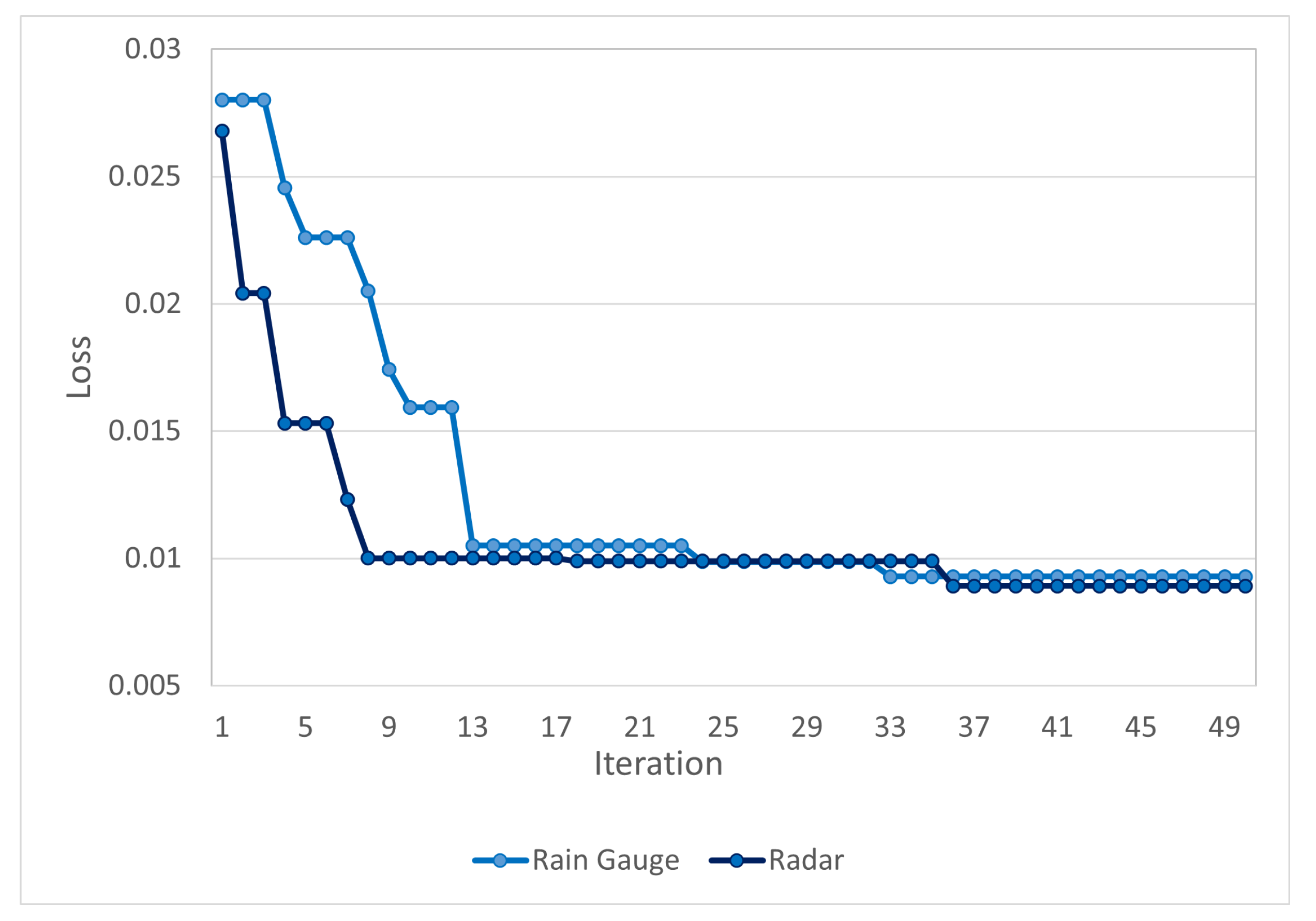
Figure 3 shows the evolution of the objective function value with PSO iterations for both rainfall inputs. The objective function decreased progressively and stabilized for both input types, reaching final values below 0.01, indicating satisfactory convergence. Notably, the radar–gauge rainfall input converged faster than the gauge-interpolated rainfall input, possibly because the higher spatial information diversity provided by radar rainfall facilitates more efficient parameter space search by the optimization algorithm.
Figure 3.
Objective function evolution during parameter optimization.
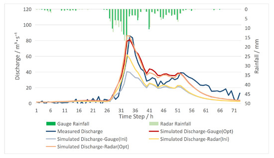
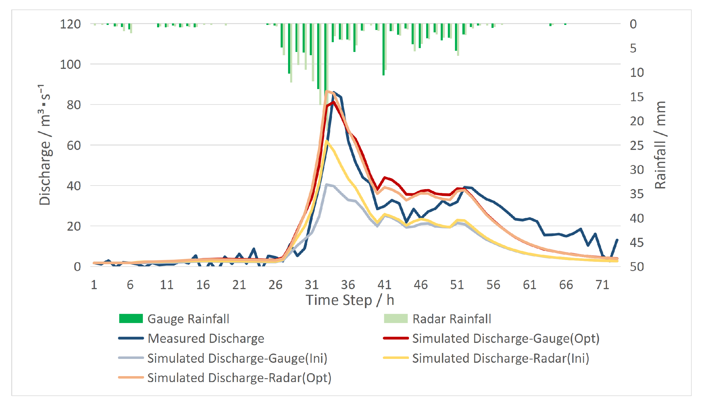
Figure 4 presents the simulated hydrographs for the calibration event 27 July 2023 using the two optimized parameter sets. Both parameter sets successfully reproduced the observed flood hydrograph. The accuracy metrics (Table 3) indicate comparable performance: NSE values of 0.831 and 0.830, KGE values of 0.868 and 0.859, correlation coefficients of 0.929 and 0.931, PRE values of 5.5% and −0.7%, and APTE values of 0 h and 1 h for gauge and radar inputs, respectively. Compared with initial (uncalibrated) parameters, parameter optimization substantially improved simulation accuracy, and the optimized parameters were subsequently applied to the validation events.
Figure 4.
Simulated hydrographs for the calibration event 27 July 2023. In the legend, Ini = initial parameters and Opt = optimized parameters obtained through PSO calibration; Gauge and Radar indicate gauge-interpolated and radar–gauge rainfall inputs, respectively.
Table 3.
Flood simulation accuracy for the calibration event.
4.2. Flood Simulation Performance Comparison
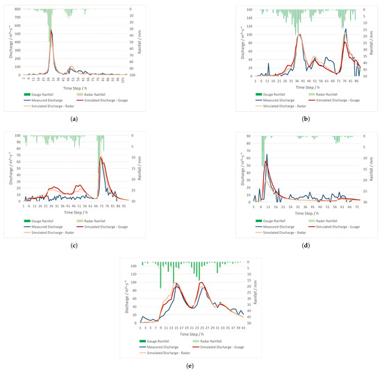
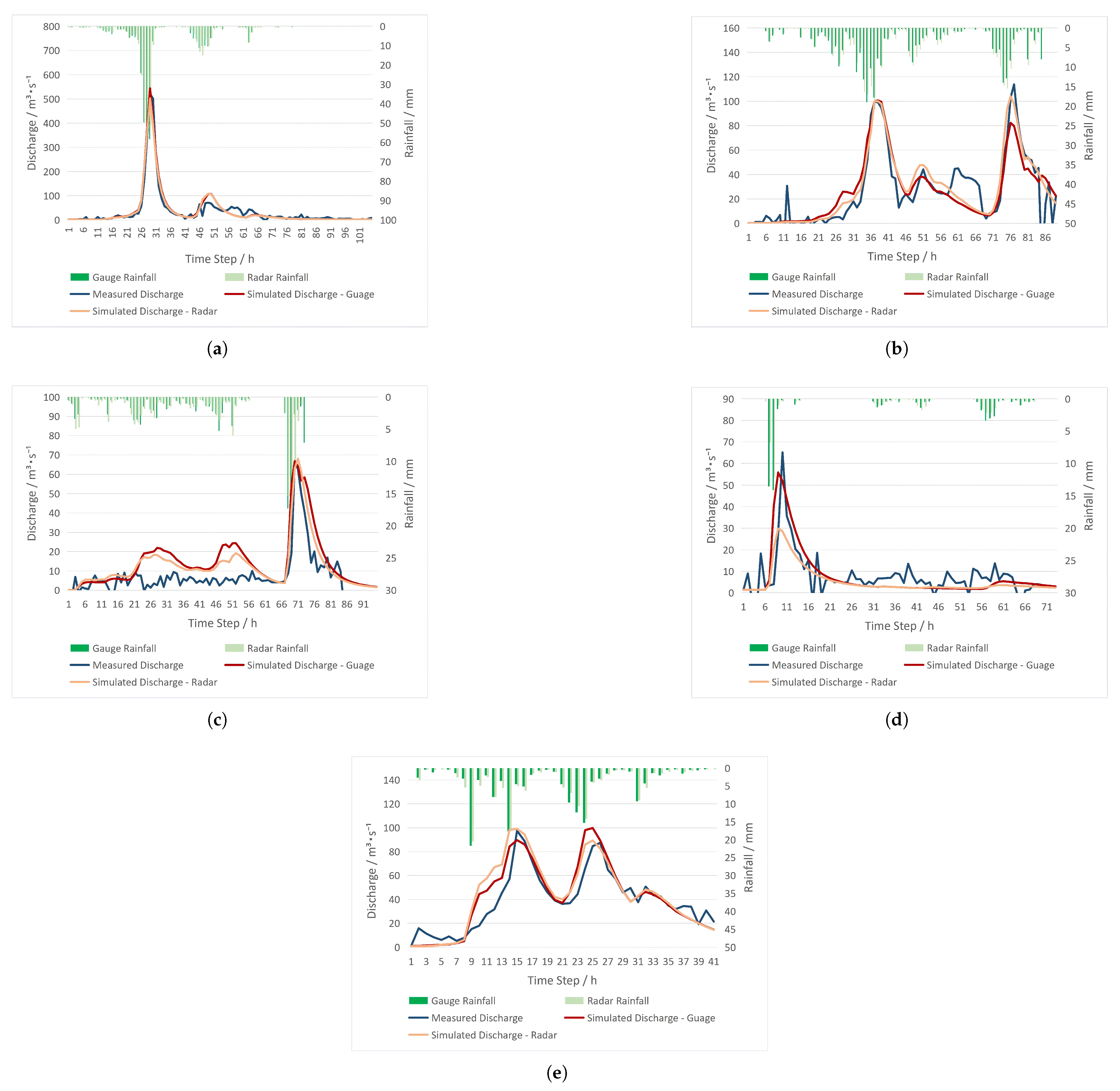
Table 4 provides the complete set of accuracy metrics for all six events, and Figure 5 displays the simulated hydrographs for the five validation flood events, comparing the two rainfall inputs.
Table 4.
Comparison of flood simulation accuracy between radar–gauge and gauge rainfall inputs.
Figure 5.
Simulated hydrographs for the validation flood events: (a) 4 September 2023; (b) 24 July 2024; (c) 21 September 2024; (d) 22 May 2025; (e) 20 July 2025.
Overall, both rainfall inputs enabled the Liuxihe model to reproduce the main hydrograph characteristics for most events. In terms of evaluation metrics, NSE exceeded 0.7 for several events, indicating the applicability of the model in the Yongtai pumped-storage catchment. However, some events showed relatively weak simulation performance, as shown in Table 4; the differences between the two rainfall inputs are detailed below.
4.2.1. Large Flood Event (4 September 2023)
For event 4 September 2023 (a large flood with peak discharge exceeding 500 m3/s), both rainfall inputs achieved high simulation accuracy, with NSE and KGE exceeding 0.9 and PRE within 5%. This indicates that under strong rainfall-driven large flood conditions, differences in spatial rainfall representation between the two input types have limited impact on simulation results.
4.2.2. Multi-Peak Flood Events (24 July 2024 and 20 July 2025)
For the two multi-peak flood events in the present dataset, the radar–gauge rainfall-driven configuration produced higher NSE and KGE values than the gauge-interpolated configuration. For event 24 July 2024, the radar–gauge configuration achieved an NSE of 0.789 and KGE of 0.863, compared with 0.732 and 0.809 for the gauge configuration; its PRE was also lower (4.7% versus 14.5%). Accurate simulation of multi-peak floods critically depends on correctly capturing the timing and magnitude of successive peaks. As simulation time progresses, rainfall input errors accumulate in the model, potentially displacing the system state. In these investigated events, the higher-resolution spatial representation of the radar–gauge input was associated with better characterization of the multi-peak response and lower cumulative error. Because the two inputs were calibrated independently, these results describe the relative performance of two operational rainfall–model configurations and cannot be attributed solely to the rainfall products.
4.2.3. Weak Rainfall Event (22 May 2025)
For event 22 May 2025 (total rainfall of only 51.1 mm), radar–gauge rainfall exhibited markedly inferior peak simulation accuracy, with a PRE of 54.1% versus 14.3% for gauge rainfall. As shown in Table 2, radar rainfall notably underestimated the total rainfall amount for this event (41.5 mm vs. 51.1 mm). This systematic underestimation of rainfall magnitude propagated through the hydrological model, resulting in a significantly underestimated simulated peak discharge.
4.3. Rainfall Spatial Variability Analysis
To investigate the underlying causes of flood simulation differences, the spatial variability of each rainfall input was quantitatively analyzed using CV and information entropy. Table 5 presents the event-weighted mean CV and H for each flood event.
Table 5.
Rainfall input spatial variability characteristics for flood events in the Yongtai pumped-storage catchment.
Radar–gauge rainfall consistently exhibited higher CV and H than gauge-interpolated rainfall across all six events, with mean increases of 34.1% and 84.4%, respectively. This indicates that the radar–gauge field has higher spatial variability and entropy-derived spatial information diversity, enabling a more detailed characterization of rainfall-field heterogeneity. For the multi-peak and localized intense-rainfall events analyzed in this study, this spatial information diversity helps explain the improved performance of the radar–gauge rainfall-driven configuration, but it is not direct evidence of higher rainfall accuracy.
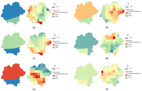
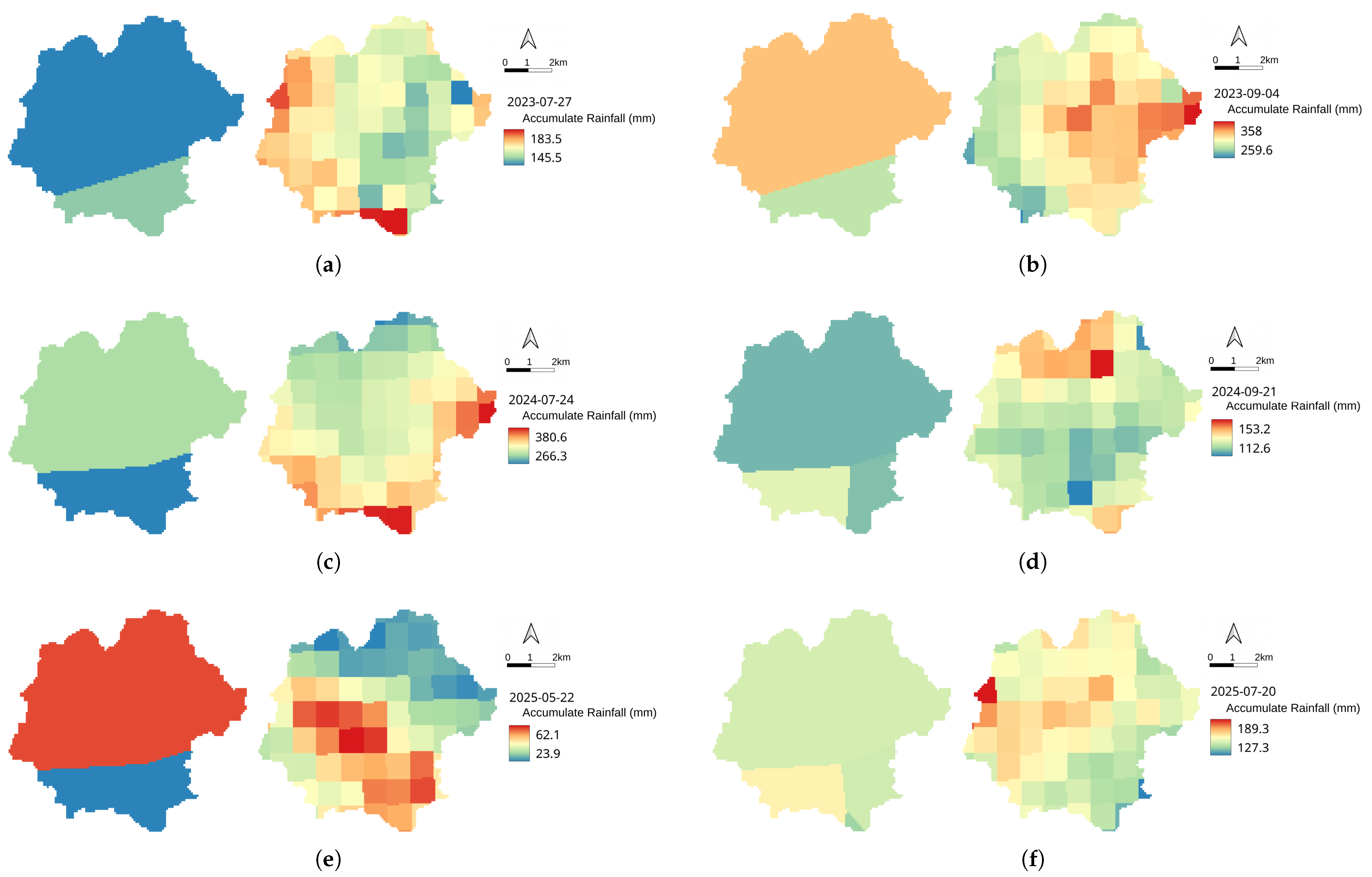
Figure 6 presents the accumulated rainfall spatial distributions for all six events, visually illustrating the differences between the two rainfall data sources.
Figure 6.
Accumulated rainfall maps: gauge-interpolated rainfall (left) and radar–gauge rainfall (right) for each flood event: (a) 27 July 2023; (b) 4 September 2023; (c) 24 July 2024; (d) 21 September 2024; (e) 22 May 2025; (f) 20 July 2025. Maps were produced using QGIS 3.40.11 and Python 3.12 (Matplotlib 3.11.1).
To further quantify the spatial characteristics of the accumulated rainfall fields, Table 6 and Table 7 present the coefficient of variation (CV) and information entropy (H) of the accumulated rainfall grids for each event under the two rainfall inputs.
Table 6.
Accumulated rainfall spatial coefficient of variation (CV).
Table 7.
Accumulated rainfall spatial information entropy (H).
Several observations emerge from the accumulated rainfall metrics. First, the CV values for accumulated rainfall (Table 6) are substantially lower than the event-weighted mean CV values reported in Table 5 (mean of 0.09 vs. 0.22–0.29), reflecting the temporal smoothing inherent in the accumulation process. The differences in accumulated CV between the two rainfall inputs are small and vary in sign across events (mean ΔCV = +0.005), indicating that the overall spatial dispersion of accumulated rainfall totals is broadly similar between the two data sources for most events. Hydrologically, a positive ΔCV indicates that radar–gauge rainfall preserves stronger accumulated-rainfall contrasts than the gauge field, whereas a negative ΔCV indicates that the gauge-interpolated field has stronger total-rainfall dispersion for that event. Notably, event 22 May 2025 exhibits the highest accumulated CV for both inputs (0.293 and 0.273), consistent with its character as a localized weak rainfall event with pronounced spatial heterogeneity.
Second, the accumulated rainfall entropy (Table 7) shows a systematic difference between the two rainfall fields. Radar–gauge rainfall exhibits H values consistently around 4.1, whereas gauge-interpolated rainfall shows H values of only 0.47–0.71, yielding a mean ΔH of +3.511. Under the present equal-width-bin framework, this difference indicates that the radar–gauge field contains a greater diversity of spatial rainfall values, whereas the Thiessen interpolation of sparse gauge observations produces a more spatially uniform field. The magnitude of the difference is also affected by the selected binning and discretization scheme; therefore, the approximately seven-fold ratio should not be interpreted as a seven-fold difference in rainfall accuracy or as an absolute measure of information content. The consistently higher H values indicate a relative difference in spatial structure under the common calculation framework, rather than intrinsic superiority of the radar–gauge product.
Third, the accumulated CV and H metrics provide complementary perspectives on rainfall spatial structure. While CV captures the relative dispersion (spread) of rainfall values, entropy captures the spatial information diversity and pattern complexity of the spatial distribution. For events such as 24 July 2024, the gauge input shows a higher accumulated CV (0.085 vs. 0.070) but much lower H (0.672 vs. 4.135), suggesting that Thiessen interpolation may produce spatially coherent structures with greater value dispersion but fewer effective value classes. This helps explain why the radar–gauge configuration can perform better in some flood simulations even when the accumulated CV does not show a clear advantage. Nevertheless, the entropy comparison is conditional on the common binning framework and should be interpreted as a diagnostic comparison of spatial structure, not as a direct accuracy ranking.
For events 27 July 2023, 4 September 2023, and 21 September 2024 (Figure 6a,b,d), the accumulated rainfall centers were relatively concentrated, and the spatial distributions of the two rainfall fields were broadly similar, with accumulated rainfall ranges of 38 mm, 98.4 mm, and 40.6 mm, indicating weak overall spatial heterogeneity. The accumulated CV values for these events are among the lowest (0.031–0.059), confirming the limited spatial contrast. In such cases, differences in spatial rainfall representation between data sources are limited, resulting in convergent flood simulation outcomes.
For the multi-peak event 24 July 2024 (Figure 6c), the accumulated rainfall center was located near the lower catchment outlet and boundary areas, exhibiting strong spatial heterogeneity with an accumulated rainfall range of 114.3 mm. The gauge network did not adequately cover this localized heavy rainfall center, and the Thiessen-interpolated rainfall field failed to capture this high-value zone, resulting in underestimated peak discharge. This error propagated through the routing process, accumulating adverse effects on successive peak simulations and further degrading overall multi-peak simulation accuracy.
For event 22 May 2025 (Figure 6e), although radar rainfall exhibited higher spatial resolution and captured more detailed rainfall patterns (CV of 0.530 vs. 0.393; H of 0.685 vs. 0.363), it systematically underestimated rainfall magnitude (radar total of 41.5 mm vs. gauge total of 51.1 mm). This indicates that while radar rainfall provides finer spatial representation and higher entropy-derived spatial information diversity, its rainfall-magnitude reliability may not necessarily exceed that of gauge observations; reliance on a single data source is inadvisable in operational flood forecasting.
For event 20 July 2025 (Figure 6f), the radar–gauge field showed an accumulated rainfall center concentrated in the upper catchment, exhibiting pronounced spatial heterogeneity, whereas the gauge-interpolated field did not represent this feature to the same extent. The resulting difference in spatial rainfall representation was associated with better characterization of the flood response in the radar–gauge configuration. This event-level result should be interpreted together with the independent calibration and the limitations of the Thiessen reference field.
Overall, the performance differences between the two rainfall–model configurations are interpreted as reflecting three main factors. First, the radar–gauge field provides higher spatial variability and entropy-derived spatial information diversity (as quantified by CV and information entropy in Table 5), enabling a more detailed characterization of spatially heterogeneous rainfall fields. Second, the Thiessen Polygon interpolation of sparse gauge observations is inherently limited in capturing localized rainfall centers, which particularly affects simulation accuracy for events with strong spatial heterogeneity and multi-peak structures. Third, radar QPE exhibits systematic underestimation under weak rainfall conditions due to Z–R relationship uncertainty and reduced signal-to-noise ratios, degrading the performance of the radar–gauge configuration for low-magnitude events. These factors collectively explain why the relative performance is strongly conditional on event characteristics and why the observed differences cannot be attributed to rainfall inputs alone.
5. Discussion
5.1. Mechanisms Underlying Conditional Rainfall–Model Configuration Performance
Because each rainfall input was calibrated independently, the results compare two operational rainfall–model configurations rather than the rainfall products in isolation. Within the available event set, the performance of the radar–gauge configuration was strongly condition-dependent and was not uniformly better than that of the gauge-interpolated configuration. The high-resolution gridded representation of the radar–gauge product provides a plausible explanation for its better metrics in some spatially heterogeneous events. As evidenced by the CV and H analyses, the radar–gauge field exhibited higher spatial variability and entropy-derived spatial value diversity across all six events, and these spatial-structure characteristics were associated with better simulation performance for some events with strong spatial heterogeneity. This association should be interpreted as correlational rather than as direct causal evidence because the optimized parameter sets also differed between configurations. The CV and H metrics are therefore used as diagnostic tools for describing rainfall-field structure, not as direct indicators of rainfall quality.
The magnitude of H also depends on the calculation framework. The continuous grid values of the radar–gauge field occupy more rainfall-value bins, whereas the Thiessen-interpolated field contains larger homogeneous zones and therefore fewer effective value classes. Consequently, the observed H difference reflects both rainfall-field structure and the selected discretization scheme. In this study, H is used only for relative comparison under the same grid and binning framework; a higher H value is not equated with higher rainfall accuracy. The configuration-level benefit was most apparent in the investigated events with localized rainfall features or multi-peak responses, for which the higher-resolution input may help the distributed model represent spatially heterogeneous runoff generation and routing.
However, radar rainfall also exhibits clear limitations. In the weak rainfall event 22 May 2025, radar systematically underestimated rainfall magnitude, substantially degrading peak simulation accuracy compared with gauge input. This phenomenon is fundamentally attributable to the uncertainties in radar QPE inversion, including Z–R relationship variability, ground clutter and beam blockage effects, and reduced signal-to-noise ratios under weak echo conditions [11,12]. Although the radar–gauge fusion product used in this study incorporates systematic bias correction, the correction constraints are limited under weak rainfall conditions, making it difficult to fully eliminate magnitude biases. In contrast, gauge observations provide higher point accuracy, and spatial interpolation effectively smooths some of the observational errors, resulting in more stable performance for this event.
5.2. Comparison with Previous Studies
The findings of this study are broadly consistent with previous research comparing radar and gauge rainfall inputs for hydrological modeling. Event-dependent benefits of radar-derived rainfall inputs under strong spatial heterogeneity have been reported in larger basins [16]; the present study examines whether similar patterns occur in a small regulated catchment under an operational independent-calibration framework. The systematic underestimation of radar QPE under weak rainfall conditions has also been documented [12], showing that such biases are not necessarily site-specific. Compared with studies that focus primarily on simulation accuracy metrics [14], the present study relates configuration-level performance differences to diagnostic measures of rainfall spatial structure (CV and information entropy), providing additional insight into why relative performance changes among events. Furthermore, this study extends our previous work in the same catchment [22], which used only gauge rainfall, by introducing radar–gauge fusion data and comparing the two operational rainfall–model configurations under a unified model structure.
5.3. Effects of Gauge Distribution on the Comparison
The spatial distribution of rain gauges in this catchment should be interpreted in relation to catchment size and station availability. During 2023, Baiyun and Xiaku provided a basic upstream–downstream coverage for the approximately 60.5 km2 catchment, corresponding to a gauge density of about 30 km2 per station, which is within the range commonly encountered in operational small mountainous catchments. The two gauges added later are relatively close to the Xiaku/lower-reservoir side; under the Thiessen Polygon method, their addition changes the interpolated rainfall spatial pattern only modestly because the adjustment is mainly local. Nevertheless, this clustered distribution still implies some spatial imbalance. This distribution has two main implications for the comparison. First, the clustered gauges provide stronger local constraints for the radar–gauge fusion near the lower/eastern part of the catchment, whereas less-gauged areas rely more heavily on radar QPE information. Second, the Thiessen interpolation based on this gauge configuration may create artificially coherent rainfall zones around gauge locations, potentially smoothing out spatial variability in less constrained areas. At the catchment outlet, the flow routing process may partially integrate and smooth these spatial biases, but localized effects on specific events remain possible. These factors should be considered when interpreting the comparative performance of the two rainfall inputs for individual events.
5.4. Limitations of This Study
Several limitations of this study should be acknowledged. First, the analysis is based on only six flood events from a single catchment, and parameter calibration used only the 27 July 2023 event. Although this event had complete observations, a moderate peak, and clearly defined rising and recession limbs, a single calibration event cannot represent the full range of rainfall intensities, antecedent soil-moisture conditions, and hydrograph types. The five validation events provide evidence of parameter transferability only within the available event set; they do not establish parameter stability across other years, catchments, or flood regimes. Multi-event calibration and validation with additional complete rainfall–runoff events are therefore needed.
Second, the rain gauge network is relatively sparse. For a small catchment of approximately 60.5 km2, the two gauges available in 2023 (Baiyun at the catchment center and Xiaku near the outlet) provide basic upstream–downstream coverage and a gauge density of about 30 km2 per station. Nonetheless, the network remains limited for resolving localized rainfall centers. Moreover, the Thiessen Polygon method partitions the catchment into homogeneous zones and cannot represent sub-catchment rainfall gradients within each zone. Accordingly, the present results compare the operational radar–gauge fusion QPE product with a specific Thiessen-interpolated gauge field; part of the observed difference may reflect the limitations of this interpolation baseline. The conclusions should not be generalized to imply that radar-based products are superior to gauge rainfall fields generated using all spatial interpolation methods. Future work should compare additional interpolation approaches when a larger observational dataset becomes available.
Third, independent parameter optimization was performed for each rainfall input, resulting in two different parameter sets. While this approach reflects common operational practice in which each input is paired with an optimized model, it introduces a confounding factor that prevents the observed performance differences from being attributed solely to rainfall data. The study therefore evaluates the attainable performance of two operational rainfall–model configurations rather than isolating the intrinsic quality of the rainfall products.
Fourth, although the two rainfall scenarios use the same model structure and underlying surface inputs (DEM, land use, soil properties), these auxiliary inputs may still influence the absolute simulation accuracy. Because they are identical across the two scenarios, they are not expected to affect the relative comparison between rainfall inputs, but spatial-resolution differences among the underlying datasets may contribute to residual uncertainty in the simulated discharge. Fifth, model performance was evaluated using deterministic metrics (NSE, KGE, PRE, and APTE). Due to the limited number of observed events and the deterministic nature of the available operational rainfall products, formal uncertainty propagation analysis was not performed in this study. Future work should incorporate additional events to better quantify model robustness under different rainfall inputs. Finally, the radar–gauge fusion product, while providing higher spatial information diversity, exhibited systematic underestimation under weak rainfall conditions, highlighting that higher spatial variability does not automatically guarantee better rainfall accuracy. These limitations notwithstanding, the present study provides a systematic comparison of two operational rainfall–model configurations in a small regulated catchment—a context that has received limited attention in the literature—and offers practical insights for rainfall-input selection. As an operational implication rather than a general guideline, a “radar-primary, gauge-auxiliary” strategy may be considered for similar data-scarce small catchments: radar–gauge fusion can provide high-resolution spatial rainfall patterns, while gauge observations remain necessary for magnitude checking and correction, especially during weak rainfall events.
6. Conclusions
This study systematically compared flood simulation performance using radar–gauge fusion and gauge-interpolated (Thiessen Polygon) rainfall inputs in the Yongtai pumped-storage hydropower catchment (∼60.5 km2) in Fujian Province, China, employing the Liuxihe distributed hydrological model. Rainfall spatial variability was quantitatively characterized using the coefficient of variation (CV) and information entropy (H). The main conclusions are as follows:
- 1.
- The Liuxihe model reproduced the main flood-process characteristics for most events under both rainfall inputs. After parameter optimization, the single calibration event (27 July 2023) achieved NSE values of 0.831 (gauge) and 0.830 (radar), and KGE values of 0.868 and 0.859, respectively. Application of the parameters to five additional events indicates a degree of transferability within the current event set.
- 2.
- Across the five validation events, both rainfall–model configurations reproduced the main hydrograph features for most events, with APTE within 1 h and PRE mostly below 15%. Under the independent-calibration framework, the radar–gauge configuration produced better metrics for event 24 July 2024 (NSE higher by 0.057, KGE higher by 0.054, and PRE lower by 9.8 percentage points), but underestimated rainfall during the weak event of 22 May 2025, resulting in poorer peak simulation (PRE of 54.1% versus 14.3% for the gauge configuration).
- 3.
- Radar–gauge rainfall exhibited consistently higher spatial variability and entropy-derived spatial value diversity than gauge-interpolated rainfall, with mean CV and H increases of 34.1% and 84.4%, respectively. Under the common calculation framework, these metrics describe relative differences in rainfall-field structure. In some events with strong spatial heterogeneity investigated in this study, higher spatial diversity was associated with better configuration-level simulation performance.
- 4.
- For the two operational configurations examined here—radar–gauge fusion QPE and Thiessen-interpolated gauge rainfall, each with independently calibrated parameters—a “radar-primary, gauge-auxiliary” multi-source strategy may be considered as a potential option for similar data-scarce small catchments. Its applicability still requires validation through multi-event calibration, additional interpolation baselines, more catchments, and more flood events.
Author Contributions
Conceptualization, Z.L., X.Y., Z.H. (Zilong Huang), Z.H. (Zhiwei Huang), J.L. and Y.C.; methodology, Z.L., X.Y., Z.H. (Zilong Huang) and Y.C.; software, Z.H. (Zilong Huang); validation, Z.L., X.Y., Z.H. (Zilong Huang), Z.H. (Zhiwei Huang), J.L. and Y.C.; formal analysis, Z.H. (Zilong Huang); investigation, Z.H. (Zilong Huang); resources, Y.C.; data curation, Z.H. (Zilong Huang); writing—original draft preparation, Z.H. (Zilong Huang); writing—review and editing, Z.L., X.Y., Z.H. (Zilong Huang), Z.H. (Zhiwei Huang), J.L. and Y.C.; visualization, Z.H. (Zilong Huang); supervision, Y.C.; project administration, Y.C.; funding acquisition, Y.C. All authors have read and agreed to the published version of the manuscript.
Funding
This research was funded by the Science and Technology Project of Fujian Yongtai Mintou Pumped-Storage Co., Ltd., grant number YT-RD-2024-001, and the National Natural Science Foundation of China, grant number U2243227.
Data Availability Statement
The hydrological data used in this study were provided by Fujian Yongtai Mintou Pumped-Storage Co., Ltd., and the radar rainfall data were provided by the Fujian Meteorological Service Center. Data are available from the corresponding author upon reasonable request.
Acknowledgments
The authors gratefully acknowledge Fujian Yongtai Mintou Pumped-Storage Co., Ltd. for providing the hydrological and rain gauge data, and the Fujian Meteorological Service Center for providing the radar–gauge fusion rainfall product. Fujian Yongtai Mintou Pumped-Storage Co., Ltd. provided data support for this study.
Conflicts of Interest
Zhihui Lin, Xiaoqi Yu, and Jize Liang are employed by Fujian Yongtai Mintou Pumped-Storage Co., Ltd. The authors declare that this study received funding from Science and Technology Project of Fujian Yongtai Mintou Pumped-Storage Co., Ltd. The funder was not involved in the study design, collection, analysis, interpretation of data, the writing of this article or the decision to submit it for publication.
Abbreviations
The following abbreviations are used in this manuscript:
| DEM | Digital Elevation Model |
| PSO | Particle Swarm Optimization |
| NSE | Nash–Sutcliffe Efficiency |
| KGE | Kling–Gupta Efficiency |
| PRE | Peak Relative Error |
| APTE | Absolute Peak Time Error |
| CV | Coefficient of Variation |
| H | Information Entropy |
| QPE | Quantitative Precipitation Estimation |
| SRTM | Shuttle Radar Topography Mission |
| SOTER | Soil and Terrain Database |
References
- Beven, K.J. Rainfall-Runoff Modelling: The Primer, 2nd ed.; Wiley-Blackwell: Chichester, UK, 2012. [Google Scholar] [CrossRef] [Scilit]
- Singh, V.P. Hydrologic Modeling: Progress and Future Directions. Geosci. Lett. 2018, 5, 15. [Google Scholar] [CrossRef] [Scilit]
- Hrachowitz, M.; Savenije, H.H.G.; Blöschl, G.; McDonnell, J.J.; Sivapalan, M.; Pomeroy, J.W.; Arheimer, B.; Blume, T.; Clark, M.P.; Ehret, U.; et al. A Decade of Predictions in Ungauged Basins (PUB)—A Review. Hydrol. Sci. J. 2013, 58, 1198–1255. [Google Scholar] [CrossRef] [Scilit]
- Refsgaard, J.C.; van der Sluijs, J.P.; Højberg, A.L.; Vanrolleghem, P.A. Uncertainty in the Environmental Modelling Process—A Framework and Guidance. Environ. Model. Softw. 2007, 22, 1543–1556. [Google Scholar] [CrossRef] [Scilit]
- Yoon, S.-S.; Lee, B. Effects of Using High-Density Rain Gauge Networks and Weather Radar Data on Urban Hydrological Analyses. Water 2017, 9, 931. [Google Scholar] [CrossRef] [Scilit]
- Hossain, F.; Anagnostou, E.N. Assessment of a Multidimensional Satellite Rainfall Error Model for Ensemble Generation of Satellite Rainfall Data. IEEE Geosci. Remote Sens. Lett. 2006, 3, 419–423. [Google Scholar] [CrossRef]
- Arnaud, P.; Bouvier, C.; Cisneros, L.; Dominguez, R. Influence of Rainfall Spatial Variability on Flood Prediction. J. Hydrol. 2002, 260, 216–230. [Google Scholar] [CrossRef] [Scilit]
- Emmanuel, I.; Andrieu, H.; Leblois, E.; Janey, N.; Payrastre, O. Influence of Rainfall Spatial Variability on Rainfall–Runoff Modelling: Benefit of a Simulation Approach? J. Hydrol. 2015, 531, 337–348. [Google Scholar] [CrossRef] [Scilit]
- Mishra, A.K. Effect of Rain Gauge Density over the Accuracy of Rainfall: A Case Study over Bangalore, India. SpringerPlus 2013, 2, 311. [Google Scholar] [CrossRef] [Scilit] [PubMed]
- Hohmann, C.; Kirchengast, G.; O, S.; Rieger, W.; Foelsche, U. Small Catchment Runoff Sensitivity to Station Density and Spatial Interpolation: Hydrological Modeling of Heavy Rainfall Using a Dense Rain Gauge Network. Water 2021, 13, 1381. [Google Scholar] [CrossRef] [Scilit]
- Sokol, Z.; Szturc, J.; Orellana-Alvear, J.; Popová, J.; Jurczyk, A.; Célleri, R. The Role of Weather Radar in Rainfall Estimation and Its Application in Meteorological and Hydrological Modelling—A Review. Remote Sens. 2021, 13, 351. [Google Scholar] [CrossRef] [Scilit]
- Tesfagiorgis, K.; Mahani, S.E.; Krakauer, N.Y.; Khanbilvardi, R. Bias Correction of Satellite Rainfall Estimates Using a Radar-Gauge Product—A Case Study in Oklahoma (USA). Hydrol. Earth Syst. Sci. 2011, 15, 2631–2647. [Google Scholar] [CrossRef] [Scilit]
- Carpenter, T.M.; Georgakakos, K.P. Impacts of Parametric and Radar Rainfall Uncertainty on the Ensemble Streamflow Simulations of a Distributed Hydrologic Model. J. Hydrol. 2004, 298, 202–221. [Google Scholar] [CrossRef] [Scilit]
- Wang, Z.; Zhong, R.; Lai, C.; Chen, J. Evaluation of the GPM IMERG Satellite-Based Precipitation Products and the Hydrological Utility. Atmos. Res. 2017, 196, 151–163. [Google Scholar] [CrossRef] [Scilit]
- Michelon, A.; Benoit, L.; Beria, H.; Ceperley, N.; Schaefli, B. Benefits from High-Density Rain Gauge Observations for Hydrological Response Analysis in a Small Alpine Catchment. Hydrol. Earth Syst. Sci. 2021, 25, 2301–2325. [Google Scholar] [CrossRef] [Scilit]
- Chen, T.; Ren, L.; Yuan, F.; Yang, X.; Jiang, S.; Tang, T.; Liu, Y.; Zhao, C.; Zhang, L. Comparison of Spatial Interpolation Schemes for Rainfall Data and Application in Hydrological Modeling. Water 2017, 9, 342. [Google Scholar] [CrossRef] [Scilit]
- Sucozhañay, A.; Célleri, R. Impact of Rain Gauges Distribution on the Runoff Simulation of a Small Mountain Catchment in Southern Ecuador. Water 2018, 10, 1169. [Google Scholar] [CrossRef] [Scilit]
- Arnaud, P.; Lavabre, J.; Fouchier, C.; Diss, S.; Javelle, P. Sensitivity of Hydrological Models to Uncertainty in Rainfall Input. Hydrol. Sci. J. 2011, 56, 397–410. [Google Scholar] [CrossRef] [Scilit]
- Fraga, I.; Cea, L.; Puertas, J. Effect of Rainfall Uncertainty on the Performance of Physically Based Rainfall–Runoff Models. Hydrol. Process. 2019, 33, 160–173. [Google Scholar] [CrossRef] [Scilit]
- Zeng, Q.; Chen, H.; Xu, C.-Y.; Jie, M.-X.; Chen, J.; Guo, S.-L.; Liu, J. The Effect of Rain Gauge Density and Distribution on Runoff Simulation Using a Lumped Hydrological Modelling Approach. J. Hydrol. 2018, 563, 106–122. [Google Scholar] [CrossRef] [Scilit]
- Huang, Z.; Chen, Y. Impact of Rain Gauge Density on Flood Forecasting Performance: A PBDHM’s Perspective. Water 2025, 17, 18. [Google Scholar] [CrossRef] [Scilit]
- Lin, Z.; Yu, X.; Huang, Z.; Huang, Z.; Wei, R.; Chen, Y. Study on Flood Forecasting Model for Small Pumped Storage Watersheds Based on the Liuxihe Model: A Case Study of the Baiyunxi Watershed. Yangtze River, 2026; in press. Available online: http://www.rmcjzz.cjw.cn/cn/article/id/b23bdd98-f5da-4526-867c-1a2371fc89a5 (accessed on 8 July 2026). (In Chinese)
- Reuter, H.I.; Nelson, A.; Jarvis, A. An Evaluation of Void-Filling Interpolation Methods for SRTM Data. Int. J. Geogr. Inf. Sci. 2007, 21, 983–1008. [Google Scholar] [CrossRef] [Scilit]
- Yang, J.; Huang, X. The 30 m Annual Land Cover Dataset and Its Dynamics in China from 1990 to 2019. Earth Syst. Sci. Data 2021, 13, 3907–3925. [Google Scholar] [CrossRef] [Scilit]
- Dijkshoorn, J.A.; van Engelen, V.W.P.; Huting, J.R.M. Soil and Landform Properties for LADA Partner Countries; ISRIC Report 2008/06; ISRIC—World Soil Information: Wageningen, The Netherlands, 2008; Available online: https://files.isric.org/public/documents/isric_report_2008_06.pdf (accessed on 8 July 2026).
- Saxton, K.E.; Rawls, W.J. Soil Water Characteristic Estimates by Texture and Organic Matter for Hydrologic Solutions. Soil Sci. Soc. Am. J. 2006, 70, 1569–1578. [Google Scholar] [CrossRef] [Scilit]
- Chen, Y.; Ren, Q.; Huang, F.; Xu, H.; Cluckie, I. Liuxihe Model and Its Modeling to River Basin Flood. J. Hydrol. Eng. 2011, 16, 33–50. [Google Scholar] [CrossRef] [Scilit]
- Chen, Y.; Li, J.; Xu, H. Improving Flood Forecasting Capability of Physically Based Distributed Hydrological Models by Parameter Optimization. Hydrol. Earth Syst. Sci. 2016, 20, 375–392. [Google Scholar] [CrossRef] [Scilit]
- Kennedy, J.; Eberhart, R. Particle Swarm Optimization. In Proceedings of the ICNN’95—International Conference on Neural Networks, Perth, WA, Australia, 27 November–1 December 1995; Volume 4, pp. 1942–1948. [Google Scholar] [CrossRef] [Scilit]
- Gupta, H.V.; Kling, H.; Yilmaz, K.K.; Martinez, G.F. Decomposition of the Mean Squared Error and NSE Performance Criteria: Implications for Improving Hydrological Modelling. J. Hydrol. 2009, 377, 80–91. [Google Scholar] [CrossRef] [Scilit]
- Nash, J.E.; Sutcliffe, J.V. River Flow Forecasting through Conceptual Models Part I—A Discussion of Principles. J. Hydrol. 1970, 10, 282–290. [Google Scholar] [CrossRef] [Scilit]
- Kling, H.; Fuchs, M.; Paulin, M. Runoff Conditions in the Upper Danube Basin under an Ensemble of Climate Change Scenarios. J. Hydrol. 2012, 424–425, 264–277. [Google Scholar] [CrossRef] [Scilit]
- Montgomery, D.C.; Runger, G.C. Applied Statistics and Probability for Engineers, 5th ed.; Wiley: New York, NY, USA, 2010. [Google Scholar]
- Shannon, C.E. A Mathematical Theory of Communication. Bell Syst. Tech. J. 1948, 27, 379–423. [Google Scholar] [CrossRef] [Scilit]
- Shannon, C.E. A Mathematical Theory of Communication. Bell Syst. Tech. J. 1948, 27, 623–656. [Google Scholar] [CrossRef] [Scilit]
- Brunsell, N.A. A Multiscale Information Theory Approach to Assess Spatial–Temporal Variability of Daily Precipitation. J. Hydrol. 2010, 385, 165–172. [Google Scholar] [CrossRef] [Scilit]

Disclaimer/Publisher’s Note: The statements, opinions and data contained in all publications are solely those of the individual author(s) and contributor(s) and not of MDPI and/or the editor(s). MDPI and/or the editor(s) disclaim responsibility for any injury to people or property resulting from any ideas, methods, instructions or products referred to in the content. |
© 2026 by the authors. Licensee MDPI, Basel, Switzerland. This article is an open access article distributed under the terms and conditions of the Creative Commons Attribution (CC BY) license.